1

Improvements to Dynamic Analysis in MSC.Nastran

P. R. Pamidi Nastran Customer Enhancements Project Manager

Mike Reymond

Nastran Rapid Response Project Manager

MSC.Software Corporation Costa Mesa, California, U.S.A.

ABSTRACT Several improvements have been made to the dynamic analysis capability in the V2001 version of MSC.Nastran with a view to enhancing its user convenience as well as functional capability. This paper discusses the details of these improvements and illustrates them by suitable examples.

2

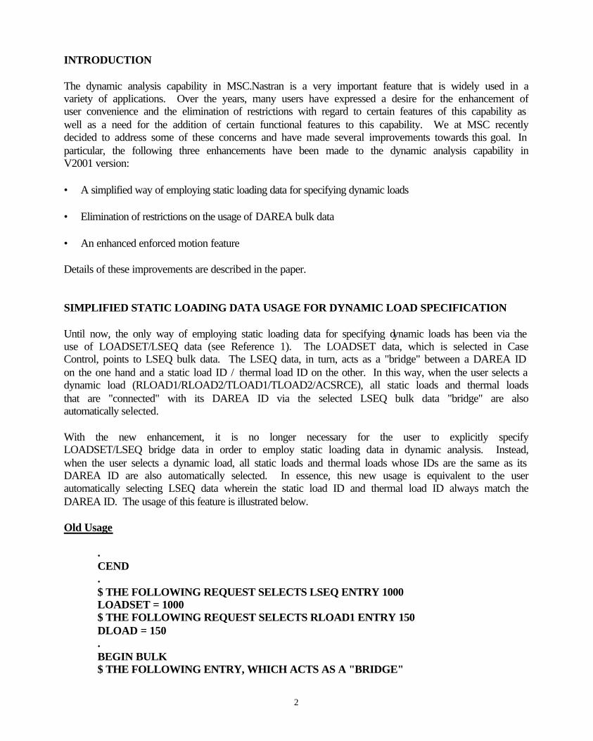
INTRODUCTION The dynamic analysis capability in MSC.Nastran is a very important feature that is widely used in a variety of applications. Over the years, many users have expressed a desire for the enhancement of user convenience and the elimination of restrictions with regard to certain features of this capability as well as a need for the addition of certain functional features to this capability. We at MSC recently decided to address some of these concerns and have made several improvements towards this goal. In particular, the following three enhancements have been made to the dynamic analysis capability in V2001 version: • A simplified way of employing static loading data for specifying dynamic loads • Elimination of restrictions on the usage of DAREA bulk data • An enhanced enforced motion feature Details of these improvements are described in the paper. SIMPLIFIED STATIC LOADING DATA USAGE FOR DYNAMIC LOAD SPECIFICATION Until now, the only way of employing static loading data for specifying dynamic loads has been via the use of LOADSET/LSEQ data (see Reference 1). The LOADSET data, which is selected in Case Control, points to LSEQ bulk data. The LSEQ data, in turn, acts as a "bridge" between a DAREA ID on the one hand and a static load ID / thermal load ID on the other. In this way, when the user selects a dynamic load (RLOAD1/RLOAD2/TLOAD1/TLOAD2/ACSRCE), all static loads and thermal loads that are "connected" with its DAREA ID via the selected LSEQ bulk data "bridge" are also automatically selected. With the new enhancement, it is no longer necessary for the user to explicitly specify LOADSET/LSEQ bridge data in order to employ static loading data in dynamic analysis. Instead, when the user selects a dynamic load, all static loads and thermal loads whose IDs are the same as its DAREA ID are also automatically selected. In essence, this new usage is equivalent to the user automatically selecting LSEQ data wherein the static load ID and thermal load ID always match the DAREA ID. The usage of this feature is illustrated below. Old Usage

. CEND . $ THE FOLLOWING REQUEST SELECTS LSEQ ENTRY 1000 LOADSET = 1000 $ THE FOLLOWING REQUEST SELECTS RLOAD1 ENTRY 150 DLOAD = 150 . BEGIN BULK $ THE FOLLOWING ENTRY, WHICH ACTS AS A "BRIDGE"

3

$ BETWEEN DAREA ID 100 AND STATIC LOAD ID 200, $ CAUSES THE SELECTION OF PLOAD4,200 LSEQ,1000,100,200 PLOAD4,200,… RLOAD1,150,100,… .

New Usage . CEND . $ THE FOLLOWING REQUEST SELECTS RLOAD1 ENTRY 150 DLOAD = 150 . BEGIN BULK $ THE FOLLOWING PLOAD4 IS AUTOMATICALLY SELECTED $ BECAUSE ITS ID OF 100 MATCHES THE DAREA ID OF THE $ SELECTED RLOAD1 ENTRY PLOAD4,100,… RLOAD1,150,100,… $ THE ABOVE USAGE IS EQUIVALENT TO THE USER $ SELECTING AN LSEQ BULK DATA OF THE FORM:- $ LSEQ,SET_ID,100,100,100 .

In order to support legacy data decks, the LOADSET/LSEQ feature will continue to be honored and supported as in earlier versions. However, the new design should obviate the need for using it in most cases. It should also be pointed out here that the new feature will be effective if and only if the user has not made a LOADSET/LSEQ selection. IMPROVEMENTS TO DAREA BULK DATA USAGE The DAREA bulk data is used to specify point loads in dynamic analysis (see Reference 1). In the case of grid points, these loads are implicitly assumed to be in the displacement (or local) coordinate systems of those points. Until now, the usage of this data in superelement analysis has been restricted to the residual. This has meant that, if users want to specify DAREA-type loads for upstream superelements, they are forced to employ equivalent FORCE/FORCE1/FORCE2, MOMENT/MOMENT1/MOMENT2 or SLOAD bulk data (as appropriate) to specify such loads. In order to avoid this drawback, an enhancement has been incorporated into the program to automatically convert internally all DAREA bulk data entries for grid and scalar points to equivalent FORCE / MOMENT / SLOAD bulk data entries (as appropriate). This scheme, in conjunction with the enhancement to static loading usage described in the earlier section, allows, for the first time, DAREA bulk data to be used for applying dynamic loads to upstream superelements in superelement analysis. The above enhancement also has two other very important advantages. These are described below.

4

• When performing dynamic analysis using the modal approach, it is very often desirable to employ residual vectors to improve the response. In addition to specifying PARAM,RESVEC,YES in the bulk data, this normally requires the user to explicitly specify static loads at those points that are dynamically excited. However, with the above automatic conversion feature, it is no longer necessary for the user to explicitly specify static loads for the purpose of residual vector calculations since such loads are automatically generated by the program.

• Until now, the usage of the DAREA bulk data has been restricted to dynamic analysis. The above

automatic conversion feature permits it, for the first time, to be used in static analysis as well. This is particularly advantageous in cases wherein the user may wish to apply loads at grid points in the displacement (or local) coordinate systems of those points.

In order to ensure that the user is kept informed of the above conversion, a message is issued at the end of the Preface informing the user of the conversion. This message also outputs a card image not only of each DAREA bulk data entry that is converted, but also of the corresponding FORCE / MOMENT / SLOAD bulk data entry to which it is converted. It should be pointed out here that the above conversion will not be performed if there is any LSEQ bulk data in the input. This is because conversion in such a case will lead to potentially wrong answers. Accordingly, the program in this case will issue an user information message indicating that the conversion is not being performed because of the presence of LSEQ bulk data in the input. ENHANCED ENFORCED MOTION FEATURE Until now, the only way of simulating enforced motion in dynamic analysis in MSC.Nastran has been via the use of large masses or the Lagrange Multiplier Technique (see Reference 2). These methods, while theoretically valid, are rather inconvenient and cumbersome for the user. The large mass method very often leads to computational and numerical problems due to round-off errors and pseudo rigid body modes. The Lagrange Multiplier Technique requires the usage of extensive DMAP alters which are difficult to maintain as newer versions of the program are released. In order to overcome these drawbacks, a new method of specifying enforced motion has been implemented. This feature permits the user to specify enforced motion in dynamic analysis directly and elegantly via SPC1/SPC/SPCD data without the need for employing large masses or the Lagrange Multiplier Technique. The program will then utilize this enforced motion information to ensure that it is properly taken into account in the analysis. The above feature is currently implemented in Solution Sequences 108, 109, 111, 112 and 200. It will be extended to nonlinear dynamic analysis in a future release of MSC.Nastran. User Interface and Specification of Enforced Motion Currently, the TYPE field (field 5) in TLOAD1 and TLOAD2 bulk data is used to indicate if the specified excitation is a force or enforced motion. This field accepts only integer values, with the following meanings:

0 (Default) Force 1 Enforced displacement using large mass

5

2 Enforced velocity using large mass 3 Enforced acceleration using large mass

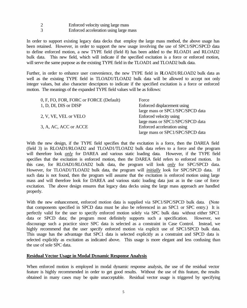
In order to support existing legacy data decks that employ the large mass method, the above usage has been retained. However, in order to support the new usage involving the use of SPC1/SPC/SPCD data to define enforced motion, a new TYPE field (field 8) has been added to the RLOAD1 and RLOAD2 bulk data. This new field, which will indicate if the specified excitation is a force or enforced motion, will serve the same purpose as the existing TYPE field in the TLOAD1 and TLOAD2 bulk data. Further, in order to enhance user convenience, the new TYPE field in RLOAD1/RLOAD2 bulk data as well as the existing TYPE field in TLOAD1/TLOAD2 bulk data will be allowed to accept not only integer values, but also character descriptors to indicate if the specified excitation is a force or enforced motion. The meanings of the expanded TYPE field values will be as follows:

0, F, FO, FOR, FORC or FORCE (Default) Force 1, D, DI, DIS or DISP Enforced displacement using large mass or SPC1/SPC/SPCD data 2, V, VE, VEL or VELO Enforced velocity using large mass or SPC1/SPC/SPCD data 3, A, AC, ACC or ACCE Enforced acceleration using large mass or SPC1/SPC/SPCD data

With the new design, if the TYPE field specifies that the excitation is a force, then the DAREA field (field 3) in RLOAD1/RLOAD2 and TLOAD1/TLOAD2 bulk data refers to a force and the program will therefore look only for DAREA and various static loading data. However, if the TYPE field specifies that the excitation is enforced motion, then the DAREA field refers to enforced motion. In this case, for RLOAD1/RLOAD2 bulk data, the program will look only for SPC/SPCD data. However, for TLOAD1/TLOAD2 bulk data, the program will initially look for SPC/SPCD data. If such data is not found, then the program will assume that the excitation is enforced motion using large mass and will therefore look for DAREA and various static loading data just as in the case of force excitation. The above design ensures that legacy data decks using the large mass approach are handled properly. With the new enhancement, enforced motion data is supplied via SPC1/SPC/SPCD bulk data. (Note that components specified in SPCD data must be also be referenced in an SPC1 or SPC entry.) It is perfectly valid for the user to specify enforced motion solely via SPC bulk data without either SPC1 data or SPCD data; the program most definitely supports such a specification. However, we discourage such a practice since SPC data is selected as a constraint in Case Control. Instead, we highly recommend that the user specify enforced motion via explicit use of SPC1/SPCD bulk data. This usage has the advantage that SPC1 data is selected explicitly as a constraint and SPCD data is selected explicitly as excitation as indicated above. This usage is more elegant and less confusing than the use of sole SPC data. Residual Vector Usage in Modal Dynamic Response Analysis When enforced motion is employed in modal dynamic response analysis, the use of the residual vector feature is highly recommended in order to get good results. Without the use of this feature, the results obtained in many cases may be quite unacceptable. Residual vector usage is triggered by specifying

6

PARAM,RESVEC,YES in the bulk data. The static loads necessary for the computations are automatically generated by the program. Improved Diagnostic Messages As part of this effort, several improvements have been made to the diagnostics resulting from a dynamic response analysis execution. These are described below. • A new user information message indicates the types of excitation specified by the user (applied

loads, enforced displacement, enforced velocity or enforced acceleration using SPC/SPCD data or large mass approach or a combination of these).

• A new user warning message is issued if any of the individual dynamic loading data results in a

null loading condition. • The execution is terminated with a user fatal error if the total excitation is null in a frequency

response analysis, thereby implying a null solution. Such a fatal error has always occurred in transient response analysis.

Procedure for Using the Enhanced Enforced Motion Feature In the light of the above discussion, the procedure for employing the enhanced enforced motion feature can be summarized as follows: 1. Specify the type of enforced motion to be applied via the TYPE field in RLOAD1/RLOAD2 (field

8) or TLOAD1/TLOAD2 (field 5) bulk data, as appropriate. 2. Define the desired enforced motion using SPCD bulk data. The set IDs of these SPCD data must

match the IDs appearing in the DAREA fields of the corresponding dynamic load data of Step 1 above.

3. Ensure that the components referenced in the SPCD data above are also specified in SPC1 bulk

data selected via Case Control. 4. If the analysis involves the modal approach, make sure that residual vectors are employed by

specifying PARAM,RESVEC,YES in the bulk data. The above enforced motion usage is illustrated below for both frequency response and transient response analyses.

7

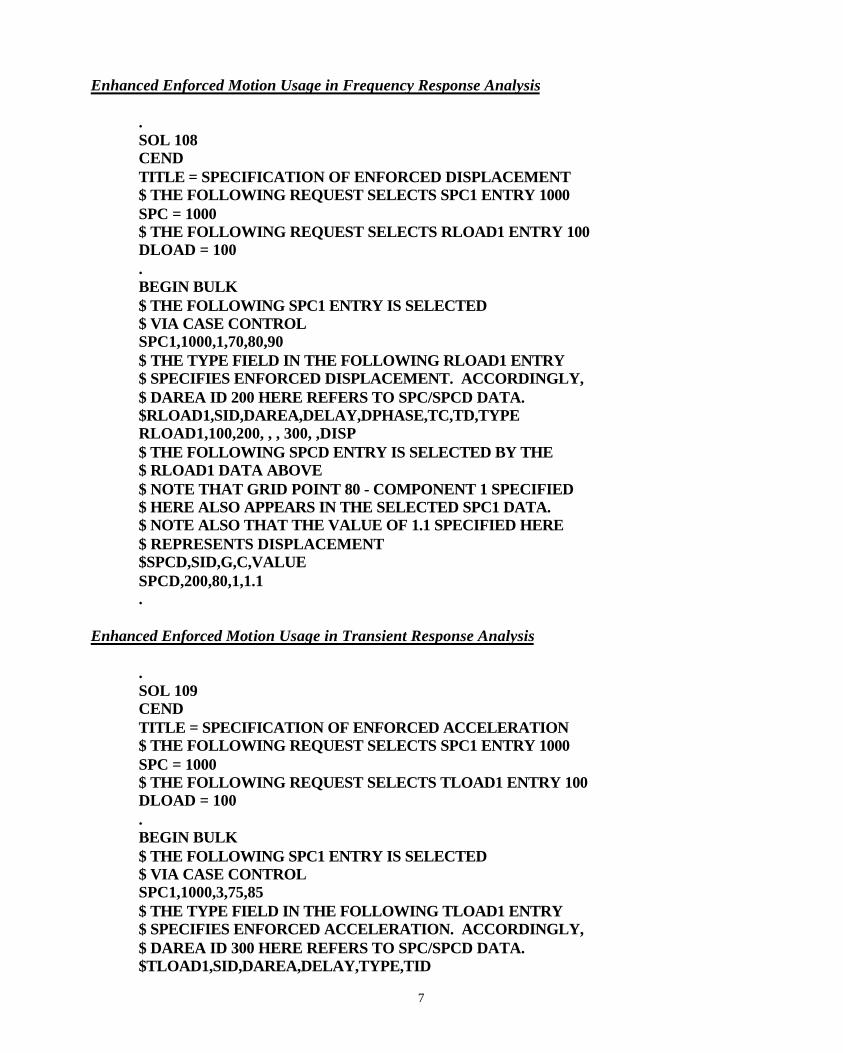
Enhanced Enforced Motion Usage in Frequency Response Analysis . SOL 108 CEND TITLE = SPECIFICATION OF ENFORCED DISPLACEMENT $ THE FOLLOWING REQUEST SELECTS SPC1 ENTRY 1000 SPC = 1000 $ THE FOLLOWING REQUEST SELECTS RLOAD1 ENTRY 100 DLOAD = 100 . BEGIN BULK $ THE FOLLOWING SPC1 ENTRY IS SELECTED $ VIA CASE CONTROL SPC1,1000,1,70,80,90 $ THE TYPE FIELD IN THE FOLLOWING RLOAD1 ENTRY $ SPECIFIES ENFORCED DISPLACEMENT. ACCORDINGLY, $ DAREA ID 200 HERE REFERS TO SPC/SPCD DATA. $RLOAD1,SID,DAREA,DELAY,DPHASE,TC,TD,TYPE RLOAD1,100,200, , , 300, ,DISP $ THE FOLLOWING SPCD ENTRY IS SELECTED BY THE $ RLOAD1 DATA ABOVE $ NOTE THAT GRID POINT 80 - COMPONENT 1 SPECIFIED $ HERE ALSO APPEARS IN THE SELECTED SPC1 DATA. $ NOTE ALSO THAT THE VALUE OF 1.1 SPECIFIED HERE $ REPRESENTS DISPLACEMENT $SPCD,SID,G,C,VALUE SPCD,200,80,1,1.1 .

Enhanced Enforced Motion Usage in Transient Response Analysis . SOL 109 CEND TITLE = SPECIFICATION OF ENFORCED ACCELERATION $ THE FOLLOWING REQUEST SELECTS SPC1 ENTRY 1000 SPC = 1000 $ THE FOLLOWING REQUEST SELECTS TLOAD1 ENTRY 100 DLOAD = 100 . BEGIN BULK $ THE FOLLOWING SPC1 ENTRY IS SELECTED $ VIA CASE CONTROL SPC1,1000,3,75,85 $ THE TYPE FIELD IN THE FOLLOWING TLOAD1 ENTRY $ SPECIFIES ENFORCED ACCELERATION. ACCORDINGLY, $ DAREA ID 300 HERE REFERS TO SPC/SPCD DATA. $TLOAD1,SID,DAREA,DELAY,TYPE,TID

8

TLOAD1,100,300, ,ACCE, 500 $ THE FOLLOWING SPCD ENTRY IS SELECTED BY THE $ TLOAD1 DATA ABOVE $ NOTE THAT GRID POINT 85 - COMPONENT 3 SPECIFIED $ HERE ALSO APPEARS IN THE SELECTED SPC1 DATA. $ NOTE ALSO THAT THE VALUE OF 2.5 SPECIFIED HERE $ REPRESENTS ACCELERATION SPCD,300,85,3,2.5 .

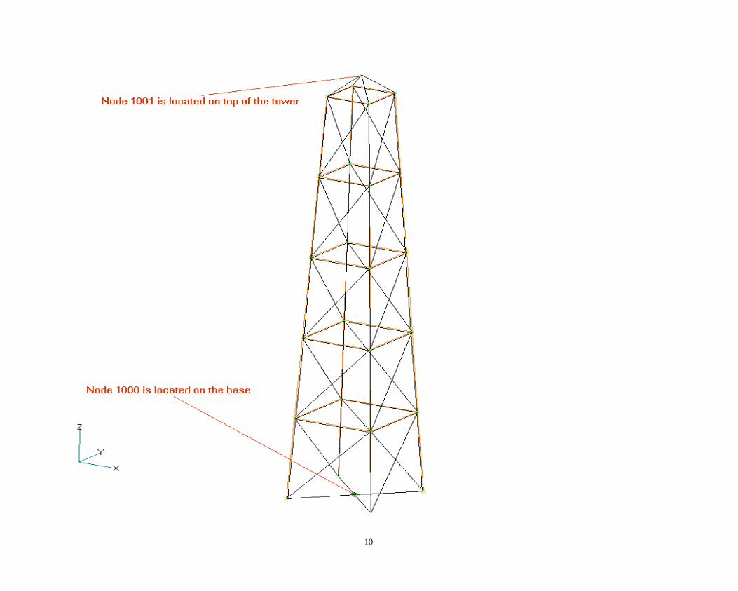
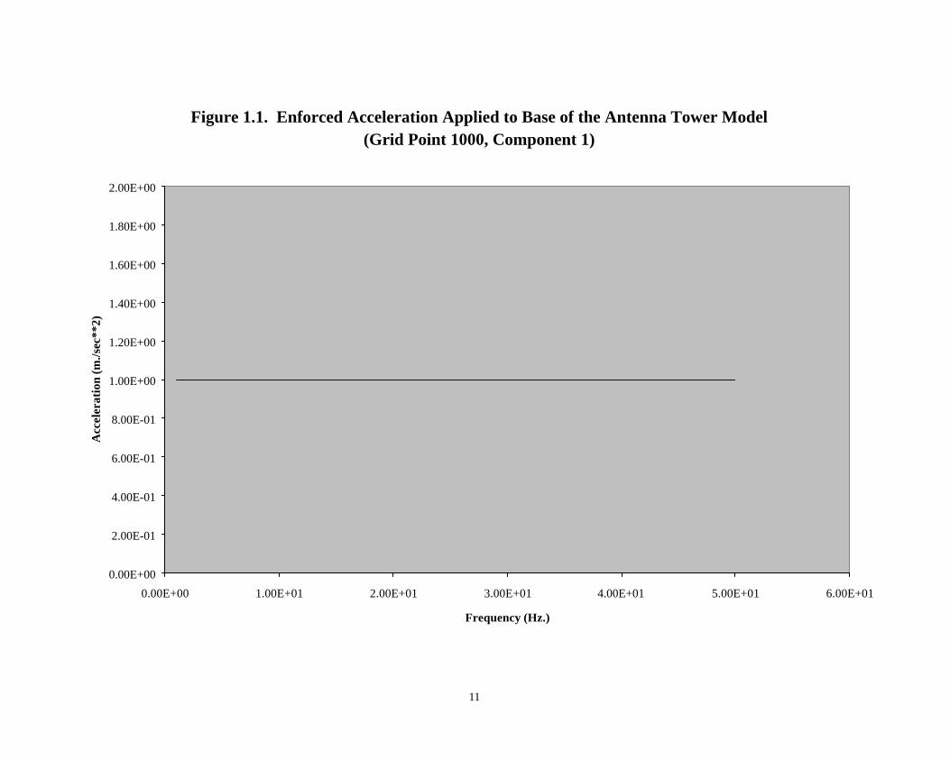
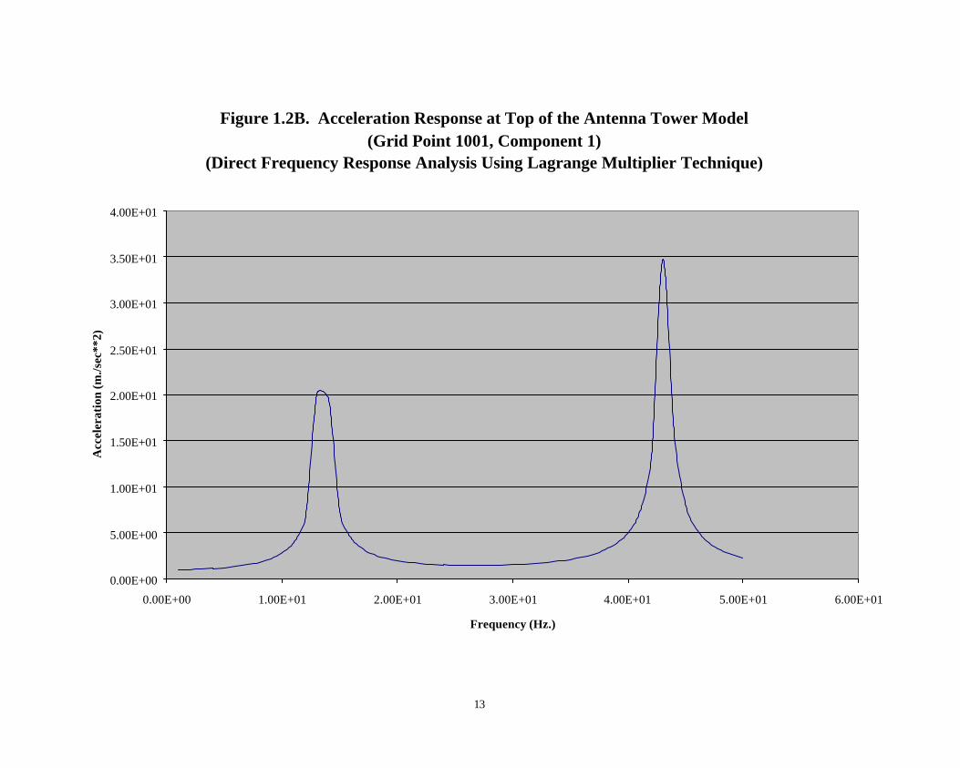
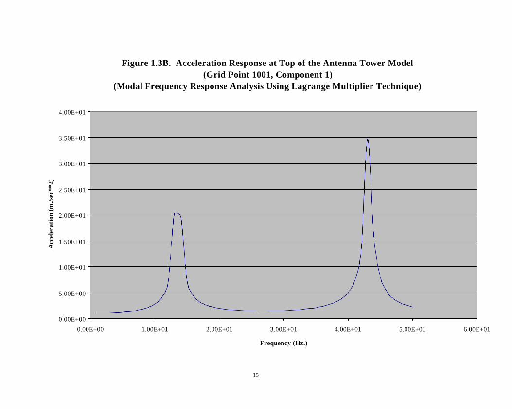
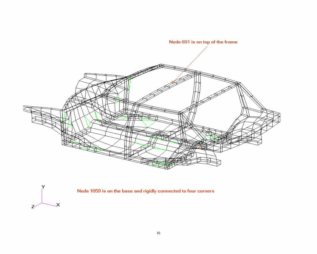
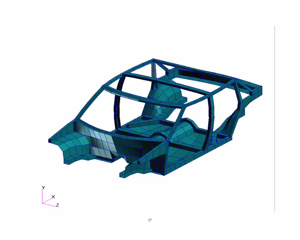
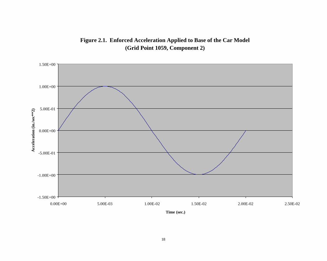
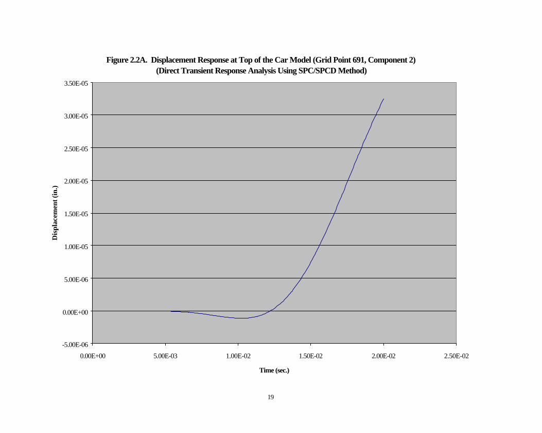
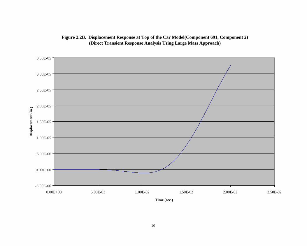
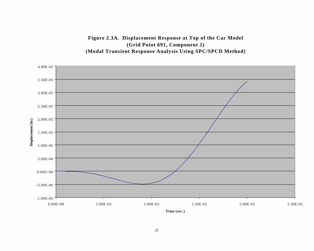
Examples of Enforced Motion Usage In order to demonstrate the enhanced enforced motion feature, we are presenting the results of two test cases. The first one is the frequency response analysis of an antenna tower with an enforced acceleration applied to the base as shown in Figure 1.1. The second one is the transient response analysis of a car with an enforced acceleration applied to the base as shown in Figure 2.1. In both cases, the analysis was performed using both direct and modal approaches. The modal approach executions employed residual vectors to get improved response as recommended earlier. The complete MSC.Nastran data decks employed for the analyses are available from the authors. For the antenna tower model, the direct frequency response results are shown in Figures 1.2A for the SPC/SPCD method and in Figure 1.2B for the Lagrange Multiplier Technique. The corresponding results for the modal frequency response are shown in Figures 1.3A for the SPC/SPCD method and in Figure 1.3B for the Lagrange Multiplier Technique. For the car model, the direct transient response results are shown in Figures 2.2A for the SPC/SPCD method and in Figure 2.2B for the large mass approach. The corresponding results for the modal transient response are shown in Figures 2.3A for the SPC/SPCD method and in Figure 2.3B for the large mass approach. The results presented demonstrate the validity of the enhanced enforced motion method described in the paper when compared to both the large mass approach and the Lagrange Multiplier Technique. CONCLUSIONS We believe that the enhancements described in this paper will be of tremendous help to users of the dynamic analysis capability in MSC.Nastran. We are currently involved in developing additional improvements as part of an ongoing effort to enhance user convenience. These features will be publicized at a later date. ACKNOWLEDGMENTS The authors wish to thank Mr. Charley Wilson, Nastran Parallel Project Manager at MSC and Mr. Mike Gockel, MSC consultant, for valuable technical discussions during the development of the enhancements. They also wish to thank Daniel Chu, Senior Client Support Engineer at MSC, for his valuable help in testing the new features described in the paper.

9

REFERENCES (1) MSC/NASTRAN Quick Reference Guide, Version 70.5, The MacNeal-Schwendler

Corporation, Los Angeles, CA, 1998. (2) MSC/NASTRAN Advanced Dynamic Analysis User's Guide, Version 70, The MacNeal-

Schwendler Corporation, Los Angeles, CA, 1997, Sections 4.2 and 4.3.

10

11

Figure 1.1. Enforced Acceleration Applied to Base of the Antenna Tower Model(Grid Point 1000, Component 1)

0.00E+00

2.00E-01

4.00E-01

6.00E-01

8.00E-01

1.00E+00

1.20E+00

1.40E+00

1.60E+00

1.80E+00

2.00E+00

0.00E+00 1.00E+01 2.00E+01 3.00E+01 4.00E+01 5.00E+01 6.00E+01

Frequency (Hz.)

Acc

eler

atio

n (m

./sec

**2)

12

Figure 1.2A. Acceleration Response at Top of the Antenna Tower Model(Grid Point 1001, Component 1)

(Direct Frequency Response Analysis Using SPC/SPCD Method)

0.00E+00

5.00E+00

1.00E+01

1.50E+01

2.00E+01

2.50E+01

3.00E+01

3.50E+01

4.00E+01

0.00E+00 1.00E+01 2.00E+01 3.00E+01 4.00E+01 5.00E+01 6.00E+01

Frequency (Hz.)

Acc

eler

atio

n (m

./sec

**2)

13

Figure 1.2B. Acceleration Response at Top of the Antenna Tower Model(Grid Point 1001, Component 1)

(Direct Frequency Response Analysis Using Lagrange Multiplier Technique)

0.00E+00

5.00E+00

1.00E+01

1.50E+01

2.00E+01

2.50E+01

3.00E+01

3.50E+01

4.00E+01

0.00E+00 1.00E+01 2.00E+01 3.00E+01 4.00E+01 5.00E+01 6.00E+01

Frequency (Hz.)

Acc

eler

atio

n (m

./sec

**2)

14

Figure 1.3A. Acceleration Response at Top of the Antenna Tower Model(Grid Point 1001, Component 1)

(Modal Frequency Response Analysis Using SPC/SPCD Method)

0.00E+00

5.00E+00

1.00E+01

1.50E+01

2.00E+01

2.50E+01

3.00E+01

3.50E+01

4.00E+01

0.00E+00 1.00E+01 2.00E+01 3.00E+01 4.00E+01 5.00E+01 6.00E+01

Frequency (Hz.)

Acc

eler

atio

n (m

./sec

**2)

15

Figure 1.3B. Acceleration Response at Top of the Antenna Tower Model(Grid Point 1001, Component 1)

(Modal Frequency Response Analysis Using Lagrange Multiplier Technique)

0.00E+00

5.00E+00

1.00E+01

1.50E+01

2.00E+01

2.50E+01

3.00E+01

3.50E+01

4.00E+01

0.00E+00 1.00E+01 2.00E+01 3.00E+01 4.00E+01 5.00E+01 6.00E+01

Frequency (Hz.)

Acc

eler

atio

n (m

./sec

**2)

16

17

18

Figure 2.1. Enforced Acceleration Applied to Base of the Car Model(Grid Point 1059, Component 2)

-1.50E+00

-1.00E+00

-5.00E-01

0.00E+00

5.00E-01

1.00E+00

1.50E+00

0.00E+00 5.00E-03 1.00E-02 1.50E-02 2.00E-02 2.50E-02

Time (sec.)

Acc

eler

atio

n (i

n./s

ec**

2)

19

Figure 2.2A. Displacement Response at Top of the Car Model (Grid Point 691, Component 2)(Direct Transient Response Analysis Using SPC/SPCD Method)

-5.00E-06

0.00E+00

5.00E-06

1.00E-05

1.50E-05

2.00E-05

2.50E-05

3.00E-05

3.50E-05

0.00E+00 5.00E-03 1.00E-02 1.50E-02 2.00E-02 2.50E-02

Time (sec.)

Dis

plac

emen

t (in

.)

20

Figure 2.2B. Displacement Response at Top of the Car Model(Component 691, Component 2)(Direct Transient Response Analysis Using Large Mass Approach)

-5.00E-06

0.00E+00

5.00E-06

1.00E-05

1.50E-05

2.00E-05

2.50E-05

3.00E-05

3.50E-05

0.00E+00 5.00E-03 1.00E-02 1.50E-02 2.00E-02 2.50E-02

Time (sec.)

Dis

plac

emen

t (in

.)

21

Figure 2.3A. Displacement Response at Top of the Car Model(Grid Point 691, Component 2)

(Modal Transient Response Analysis Using SPC/SPCD Method)

-1.00E-05

-5.00E-06

0.00E+00

5.00E-06

1.00E-05

1.50E-05

2.00E-05

2.50E-05

3.00E-05

3.50E-05

4.00E-05

0.00E+00 5.00E-03 1.00E-02 1.50E-02 2.00E-02 2.50E-02

Time (sec.)

Dis

plac

emen

t (in

.)

22

Figure 2.3B. Displacement Response at Top of the Car Model(Grid Point 691, Component 2)

(Modal Transient Response Analysis Using Large Mass Approach)

-1.00E-05

-5.00E-06

0.00E+00

5.00E-06

1.00E-05

1.50E-05

2.00E-05

2.50E-05

3.00E-05

3.50E-05

4.00E-05

0.00E+00 5.00E-03 1.00E-02 1.50E-02 2.00E-02 2.50E-02

Time (sec.)

Dus

plac

emen

t (in

.)