NaSt3DGP - Research Group Prof. Griebelwissrech.ins.uni-bonn.de/research/projects/NaSt3DGP/... ·...

NaSt3DGP

A Parallel 3D Navier-Stokes Solver

User’s Guide

Institute of Numerical SimulationDivision of Scientific Computing and Numerical Simulation

University of Bonn

Michael Griebel, Roberto Croce, Martin Engel

http://wissrech.iam.uni-bonn.de/research/projects/NaSt3DGP/index.htmContact: [email protected]

Contents

1 Introduction 5

2 Installation 7

2.1 The build and install process on UNIX platforms . . . . . . . . . . . . . . 7

2.2 Build and install on Windows . . . . . . . . . . . . . . . . . . . . . . . . . 12

2.3 Additional remarks and known problems . . . . . . . . . . . . . . . . . . . 12

2.3.1 Known issues . . . . . . . . . . . . . . . . . . . . . . . . . . . . . . 12

2.4 Running a first example . . . . . . . . . . . . . . . . . . . . . . . . . . . . 13

3 Numerical Method 19

3.1 The Projection-Method . . . . . . . . . . . . . . . . . . . . . . . . . . . . . 20

3.2 The Boussinesq-Approximation . . . . . . . . . . . . . . . . . . . . . . . . 20

3.3 Time discretization . . . . . . . . . . . . . . . . . . . . . . . . . . . . . . . 21

3.4 Boundary conditions . . . . . . . . . . . . . . . . . . . . . . . . . . . . . . 21

3.5 Computational grid and spatial discretization . . . . . . . . . . . . . . . . 22

3.6 Discretization of boundary conditions . . . . . . . . . . . . . . . . . . . . . 25

4 Navcalc and Navcalcmpi 27

4.1 Command line arguments . . . . . . . . . . . . . . . . . . . . . . . . . . . 27

4.2 Parallelization issues . . . . . . . . . . . . . . . . . . . . . . . . . . . . . . 27

4.3 Implementational details . . . . . . . . . . . . . . . . . . . . . . . . . . . . 28

5 Navsetup 33

5.1 Command line arguments . . . . . . . . . . . . . . . . . . . . . . . . . . . 33

5.2 Scene description file . . . . . . . . . . . . . . . . . . . . . . . . . . . . . . 35

5.2.1 Blocks . . . . . . . . . . . . . . . . . . . . . . . . . . . . . . . . . . 35

5.2.2 Comments . . . . . . . . . . . . . . . . . . . . . . . . . . . . . . . . 35

5.2.3 dimension . . . . . . . . . . . . . . . . . . . . . . . . . . . . . . . . 35

5.2.4 parameter . . . . . . . . . . . . . . . . . . . . . . . . . . . . . . . . 36

5.2.5 Objects . . . . . . . . . . . . . . . . . . . . . . . . . . . . . . . . . 42

3

4 CONTENTS

6 Utilities 476.1 vrml2nav . . . . . . . . . . . . . . . . . . . . . . . . . . . . . . . . . . . . . 476.2 GridGen . . . . . . . . . . . . . . . . . . . . . . . . . . . . . . . . . . . . . 496.3 Interface to MatLab . . . . . . . . . . . . . . . . . . . . . . . . . . . . . . 506.4 Interface to VTK . . . . . . . . . . . . . . . . . . . . . . . . . . . . . . . . 51

7 Examples 537.1 Lid-driven cavity . . . . . . . . . . . . . . . . . . . . . . . . . . . . . . . . 53

8 In case of Trouble 578.1 Submitting bug reports . . . . . . . . . . . . . . . . . . . . . . . . . . . . . 57

9 License 59

Chapter 1

Introduction

NaSt3DGP is a C++ implementation of a solver for the incompressible, time-dependentNavier-Stokes equations in three dimensions. It is based on a Chorin-type projectionmethod and uses finite difference approximations for the spatial derivatives on non-uniformstaggered meshes. Among the implemented features are Adams-Bashforth and Runge-Kutta methods for handling of the time derivatives and various upwind schemes likeQUICK, SMART and VONOS for discretization of the convective terms. The calculationof temperature or concentration fields within the flow is also possible.The code can be compiled to get a parallel version based on the message passing interfaceMPI, or to get a single processor version, which does not require any installation of MPI.NaSt3DGP provides a user-friendly interface to describe the geometry and the variousproblem dependent parameters by a macro language. This interface also provides importand export capabilities for the numerical results. In addition, NaSt3DGP includes someutilities for the generation of smooth non-uniform grids and for the import and export ofnumerical results from/to various other software packages such as MatLab or Tecplot.

The remainder of this guide is as follows.

Chapter 2 explains the installation of NaSt3DGP and the basic usage is shown for thestandard testcase of Driven-Cavity flow.

Chapter 3 describes the numerical scheme. This includes the description of the differencestencils used for the spatial discretization and the boundary conditions.

Chapter 4 introduces navcalc and navcalcmpi - the parts of NaSt3DGP which actuallyperform the numerical simulations. A basic outline of the implementation is given. Thisshould help users to adapt the code for their own purposes if necessary.

Chapter 5 deals with navsetup - the interface tool. First the command line argumentsare introduced. navsetup is able to read so-called scene description files which describedifferent parameters of the flow, the spatial discretization and a description of the geometryof the domain using a simple macro language. The key words of this language are given insubsection 5.2.

5

6 CHAPTER 1. INTRODUCTION

Chapter 6 explains various utilities that come with NaSt3DGP.

Chapter 7 shows some example simulations done with NaSt3DGP. The scenefiles for thesesimulations are included in the distribution.

Chapter 8 describes how to report bugs.

Chapter 9 contains the license under which NaSt3DGP is made available.

Chapter 2

Installation

NaSt3DGP uses the GNU autoconf and automake installation mechanism. Therefore, onmost UNIX systems and on the Cygwin platform running under Windows, the usual pro-cess of

./configure

make

make install

should work. Detailed installation instructions and options to the configure script are givenin the following sections.

2.1 The build and install process on UNIX platforms

NaSt3DGP is distributed as a standard UNIX tarball. First, you need to unpack the dis-tribution. Depending on your version of tar, you can use one of the following commandsto unpack the tarball to the current directory.

gzip -dc nast3dgp.tar.gz | tar xvf -

or

tar xvzf nast3dgp.tar.gz (if your version of tar support this).

Now change into the created subdirectory nast3dgp and issue the following command:

./configure [OPTIONS]

7

8 CHAPTER 2. INSTALLATION

The command

./configure --help

will give you a complete list of available options with a short help message. The mostimportant and NaSt3DGP-specific options are shown in table 2.1. Each option has a defaultvalue (also given in table 2.1) which will be used if you do not specify the correspondingoption. Table 2.2 lists other available configure options.

Table 2.1: Some useful options to configure.

--prefix=PREFIX with this option you can control where NaSt3DGP will be in-stalled when the make install command is issued. PREFIX isa directory. You need write-access to PREFIX when installingthe program. The default value for PREFIX is /usr/local/.

--enable-mpi with this option you control whether the parallel version ofNaSt3DGP based on MPI will be built. You need a properinstallation of an MPI implementation for this to work. The de-fault value is always yes, if configure can detect an installationof MPI(configure tries to do this when running). If the configurescript is unable to find a MPI installation, parallel build will bedisabled. You can explicitly disable building the parallel versionof NaSt3DGP by specifying --disable-mpi.

--enable-timer with this option you control the output of timing information. Ifenabled, additional profiling information will be generated. Thedefault value is no. (Remark: this switch affects only the parallelversion, it is ignored when building the serial version.

--with-docdir=DIR with this option you can specify a separate directory for instal-lation of the documentation. The default value for DIR is [PRE-FIX/share/doc/nast3dgp].

Further finetuning of the build process can be achieved by supplying additional environ-ment variables on the configure command-line, i.e.

./configure [OPTIONS] VAR=VALUE

See table 2.3 for a list of used environment variables.

Perhaps the most important variable is CXXFLAGS. You can use it for instance to controlthe level of optimization(default optimization level depends on the compiler detected byconfigure, for GNU compilers it is usually -O2). For example, on a Linux system running

2.1. THE BUILD AND INSTALL PROCESS ON UNIX PLATFORMS 9

Table 2.2: Some more options to configure.

-h, --help display this help and exit--help=short display options specific to this package--help=recursive display the short help of all the included pack-

ages-V, --version display version information and exit-q, --quiet, --silent do not print ‘checking...’ messages--cache-file=FILE cache test results in FILE [disabled]-C, --config-cache alias for ‘–cache-file=config.cache’-n, --no-create do not create output files--srcdir=DIR find the sources in DIR [configure dir or ‘..’]--prefix=PREFIX install architecture-independent files in PRE-

FIX [/usr/local]--exec-prefix=EPREFIX install architecture-dependent files in EPRE-

FIX [PREFIX]--bindir=DIR user executables [EPREFIX/bin]--sbindir=DIR system admin executables [EPREFIX/sbin]--libexecdir=DIR program executables [EPREFIX/libexec]--datadir=DIR read-only architecture-independent data [PRE-

FIX/share]--sysconfdir=DIR read-only single-machine data [PREFIX/etc]--sharedstatedir=DIR modifiable architecture-independent data

[PREFIX/com]--localstatedir=DIR modifiable single-machine data [PREFIX/var]--libdir=DIR object code libraries [EPREFIX/lib]--includedir=DIR C header files [PREFIX/include]--oldincludedir=DIR C header files for non-gcc [/usr/include]--infodir=DIR info documentation [PREFIX/info]--mandir=DIR man documentation [PREFIX/man]--program-prefix=PREFIX prepend PREFIX to installed program names--program-suffix=SUFFIX append SUFFIX to installed program names--program-transform-name=PROGRAM run sed PROGRAM on installed program

names


on a pentium class or higher processor, you could use the following command:

./configure [OPTIONS] CXXFLAGS=’-Wall -ansi -O3 -mcpu=pentiumpro -ffast-math

-funroll-loops’

By default, configure picks the first compiler it detects on the hosts system. With thevariable CXX you can explicitly specify the C++-compiler which should be used during thebuild process.In order to build a parallel version of NaSt3DGP (see option --enable-mpi in table 2.1)you need a proper installation of an MPI implementation. You can download the free MPI

implementation MPICH from the Computer Science Division of the Argonne NationalLaboratory http://www-unix.mcs.anl.gov/mpi/mpich/.By specifying the variables MPICXX and MPILIBS you can build a parallel version of NaSt3DGPeven if the configure script could not detect an installation of MPI in one of the standardlocations. With some versions of MPI you can use the variable MPICXX to force the usagefo a specific C++-Compiler, for example

./configure [YOUROPTIONS] MPICXX=’mpiCC -CC=/path/to/your/compiler/bin/g++’

For driver-scripts which do not support the -CC option (usually the driver-scripts of SCoredon’t) you might use the following workaround: just make sure that the compiler you wantto use is the first to appear in your path, that is the one some driver-script use (e.g. SCoreversion 5 does).

After a successfull run of configure, just type

make

ormake -j 2

if building on a 2-processor machine. After the build process has successfully finished, type

make install

to install NaSt3DGP into PREFIX, where PREFIX is the directory you specified with the–prefix option when configuring. After installation you will find the following subdirectoriesand files located under PREFIX:

• in PREFIX/bin you will find the binaries navsetup, vrml2nav, navcalc and alsonavcalcmpi if the parallel version was built. navsetup is a multi-purpose interfacetool for generating input files for navcalc and generating output for visualization.

2.1. THE BUILD AND INSTALL PROCESS ON UNIX PLATFORMS 11

Table 2.3: Additional environment variables for configure.

CXX specify a C++ compiler other than the one detected by con-figure

CXXFLAGS flags for the default compiler or the one specified with CXX

LDFLAGS linker flags, e.g. -L 〈lib dir〉 if you have libraries in a nonstan-dard directory 〈lib dir〉

CPPFLAGS C/C++ preprocessor flags, e.g. -I 〈include dir〉 if you haveheaders in a nonstandard directory 〈include dir〉

CC C compiler commandCFLAGS C compiler flagsCXXCPP C++ preprocessorMPICXX MPI C++ compiler commandMPILIBS necessary libraries to link MPI C code

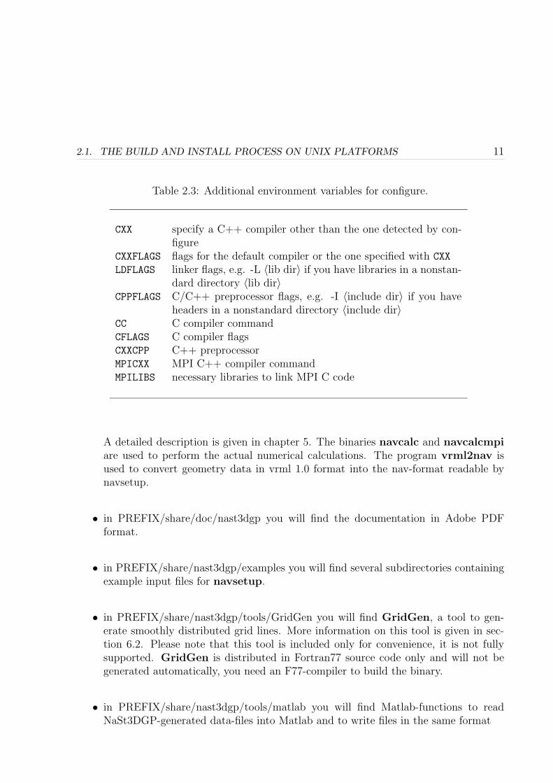
A detailed description is given in chapter 5. The binaries navcalc and navcalcmpiare used to perform the actual numerical calculations. The program vrml2nav isused to convert geometry data in vrml 1.0 format into the nav-format readable bynavsetup.

• in PREFIX/share/doc/nast3dgp you will find the documentation in Adobe PDFformat.

• in PREFIX/share/nast3dgp/examples you will find several subdirectories containingexample input files for navsetup.

• in PREFIX/share/nast3dgp/tools/GridGen you will find GridGen, a tool to gen-erate smoothly distributed grid lines. More information on this tool is given in sec-tion 6.2. Please note that this tool is included only for convenience, it is not fullysupported. GridGen is distributed in Fortran77 source code only and will not begenerated automatically, you need an F77-compiler to build the binary.

• in PREFIX/share/nast3dgp/tools/matlab you will find Matlab-functions to readNaSt3DGP-generated data-files into Matlab and to write files in the same format


2.2 Build and install on Windows

Since NaSt3DGP is developed mainly on Unix-based systems the support for Windows isvery rudimentary. We only provide a simple Makefile for the MS VC5 compiler which canbe used with nmake. The file Makefile.VC5 is included in the distribution in the directoryNaSt3DGP/src.Another way to use NaSt3DGP on Windows machines is to install a Cygwin-Environment.You can download Cygwin for free from http://www.cygwin.com. If you use it, simplyfollow the build process as described in the Unix-section.

2.3 Additional remarks and known problems

The current release of NaSt3DGP is known to succesfully install at least on the followingsystems and platforms:

• Intel 32-bit

– Redhat Linux 7.2 with libc 2.2.4 and gcc versions 2.96, SCore 2.4.1

– Redhat Linux 7.3 with libc 2.2.x and gcc 3.2, SCore 5.4

– Redhat Linux 7.3 with libc 2.2.x and gcc 3.2, SCore 5.4

– Redhat Linux 9.0 with libc 2.3.2 and gcc 3.0 or higher, MPICH 1.2.5

– Debian 3.0 with libc 2.3.2 and gcc 3.2, MPICH 1.2.5

– Redhat Linux 9.0 with libc 2.3.2 and icc 7.1 Build 20030822Z (Remarks: dueto a bug in this and prior versions of icc, dependency tracking may not be fullyfunctional)

• Intel 64-bit (Itanium)

– Debian Linux with libc 2.2.5 and gcc 3.2, MPICH 1.2.5

2.3.1 Known issues

Some versions of MPICH and SCore provide buggy driver-scripts for the compiler. Thescripts parse the command-line and alter it before handing it down to the actual com-piler. This may lead to a false assumption about the style of dependency tracking. As aconsequence, rebuilds of the source may fail with an error message similar to

cpp0: you must additionally specify either -M or -M

If this happens, there are several possible work-arounds and fixes:

2.4. RUNNING A FIRST EXAMPLE 13

• in the subdirectories mpi/ and src/ of the build-tree, delete the object files producingthe error, that is, the ones corresponding to the source files that were changed, thenrebuild with make

• supply the driver-script as the CXX compiler, i.e. use ./configure [YOUROPTIONS]

CXX=mpiCC

• disable dependency tracking by using the switch --disable-dependency-tracking

when running configure.

• patch the driver scripts mpic++ and mpiCC (when using SCore, they are located in a di-rectory similar to /opt/score/mpi/mpich-1.2.4/i386-redhat7-linux2 4 gnu/bin

2.4 Running a first example

In this section the general usage of the software package NaSt3DGP is shown, involvingall the steps from generating an input file until visualising the final output. For detailedinformation on the usage of navsetup and navcalc/navcalcmpi please refer to the corre-sponding chapters of this manual. Both programs show a basic help message when calledwith the option -h.

First, choose a directory where you want to store and and work with the generated data, e.g./home/my home/Nast-Examples. Change to this directory and copy the file cavity.nav

from PREFIX/share/nast3dgp/examples/Cavity2D into this directory. The format andall parameters of this file are described in detail in section 5.2. Now execute navsetup inthe following way:

navsetup -s cavity.nav -b cavity.bin

Remark: Depending on the installation PREFIX you choose, you may have to call navsetupwith the complete path, i.e. PREFIX/bin/navsetup or else include the directory PRE-FIX/bin into your PATH environment variable. This holds for all subsequent calls tobinaries of the NaSt3DGP package.

The setup program navsetup reads the configuration file cavity.nav which contains allnecessary parameters for the description of the ’Driven Cavity’-testcase and generates abinary data file cavity.bin. This binary file contains all the data required for the subsequentcomputation with navcalc, i.e. the computational grid, initial values for u and p and othernecessary parameters. The generated binary file can be used for both serial and parallelcomputations.

To start the actual simulation, use the command


Table 2.4: Sample output at startup of navcalc.

Reading file cavity.bin...

Time: 0, finish at 0.2

Gridpoints: 5120 (32x32x5), containing 0 obstacle cells

maxgridsize=0.03125 mingridsize=0.03

eps=1e-08 omg=1.7 alpha=0 alphatg=1

tfdiff=0.5 tfconv=0.5

reynolds=1000 froude=1

gx=0 gy=0 gz=0

temperature is not calculated

chemicals are not calculated

periodic bound in z-direction.

time handling: Runge-Kutta 3rd

iteration scheme: BiCGStab

convective terms handling: VONOS

navcalc -b cavity.bin -p3

for the serial version and the following one for running a parallel calculation on 2 processors:

mpirun -np 2 navcalcmpi -b cavity.bin -p3

Remark: the actual command for running a parallel calculation may differ from the oneabove, depending on your installation of MPI.The first calculation runs only for ten timesteps in order to get results quickly.

At the beginning, navcalc prints some information on the calculation it is about to perform,you can use this output to check if the most important parameters in the scene descriptionfile are set correctly. When running in parallel mode, additional output about the distri-bution on different processors/machines is displayed. Sample output looks similar to theone shown in tables 2.4 and 2.5.During the calculation navcalc prints some information on the screen(table 2.6), e.g. theactual time, the size of the timestep, the divergence of the velocity field and informationabout the residuals of the pressure poisson equation.

When the final time is reached, the data file cavity.bin is overwritten with the calculateddata from the final time. The command


Table 2.5: Additional output of navcalcmpi.

2 (1/2/1) procs, I am 1 (0/1/0) (yourhost.yourdomain),

neighbours N:-1 S:-1 W:-1 E: 0 T:-1 B:-1.

Process 1 (1-32, 17-32, 1-5) CompTemp:0 CompFrBd:0 CompChem:0 nChem:0

Number of started processes 2

2 (1/2/1) procs, I am 0 (0/0/0) (yourhost.yourdomain),

neighbours N:-1 S:-1 W: 1 E:-1 T:-1 B:-1.

Process 0 (1-32, 1-16, 1-5) CompTemp:0 CompFrBd:0 CompChem:0 nChem:0

Init. Arrays

iobc1_vol: 0.000000e+00

volume of domain = 1.500000e-01

Build local Lists 0

inflow_surface = 0.075 outflow_surface = 0 flow_in = 0

Initialization done 0

Table 2.6: Runtime information of navcalc/navcalcmpi.

Step: 418 Time: 8.360000 TimeStep: 0.02000000000000 Time: 0h 5m 49.62s

it: 1 res: 1.332181e-04 itmax: 100

it: 51 res: 1.254539e-07 itmax: 100

Iter: 88 Res: 4.54237223e-09 all It: 38306

Mass Balance (rhs): 2.11625890e-01

Mass Balance (aps): 4.54237223e-09

flow_in=0 flow_out=0 mass_diff=0

Output...

Step: 419 Time: 8.380000 TimeStep: 0.02000000000000 Time: 0h 5m 50.27s

it: 1 res: 1.299858e-04 itmax: 100

it: 51 res: 1.233602e-07 itmax: 100

Iter: 85 Res: 9.69241550e-09 all It: 38391

Mass Balance (rhs): 2.11616888e-01

Mass Balance (aps): 9.69241550e-09

flow_in=0 flow_out=0 mass_diff=0

Output...


Figure 2.1: Contour lines of u,v and p (left to right) at time t = 0.1.

Figure 2.2: Streamlines and velocity vectors at time t = 0.1.

navsetup -TC cavity.bin -o results

generates a file named results.dat which is suitable for processing with Tecplot. TheNaSt3DGP package supports several different output formats, e.g. for Matlab or VTK1.For details about different data conversion possibilities of navsetup, refer to chapter 5.

The results for the first, very short simulation are shown in figures 2.1 and 2.2.

Now edit the scene description file cavity.nav and increase the simulation time by set-ting a value of 250 for Tfin. Rerun this example by following the steps above for thenew cavity.nav file2. Now the flof pattern does look like what you would expect for the

1The Visualization ToolKit, a C++ class library available at http://public.kitware.com/VTK/2of course increasing the final time results in a longer computing time, on a 2-processor Xeon 933MHz

machine the simulation takes about three quarters of an hour


Figure 2.3: Contour lines of u,v and p (left to right) in steady state (time t = 250).

Figure 2.4: Streamlines and velocity vectors in steady state (time t = 250).

’Driven Cavity’-problem, since the solution has reached the steady state (see [1] or [4]).Visualizations of the result done with Tecplot are shown in figures 2.3 and 2.4.

More examples are presented in chapter 7. See section 5.2 for details on the format of thescene description file to design your own problem descrption files.

Chapter 3

Numerical Method

In this chapter we give a brief description of the numerical method underlying NaSt3DGP.For more information please refer to [1]. In several cases, different numerical methods,for example, different discretizations for time derivatives or convective terms, are possible.Details on how to control these schemes using the scene description file are given in section5.2.The basic mathematical model are the dimensionless time-dependent incompressible Navier-Stokes equations

∂u

∂t+ u · ∇u =

g

Fr−∇p+

1

Re∆u , x ∈ Ω, 0 ≤ t ≤ Tfin (3.1)

∇ · u = 0 , (3.2)

subject to appropriate initial and boundary conditions. Re is the dimensionless Reynolds-number which determines the ration between inertia and viscous forces in the flow. theReynolds-number is given by

Re =ρLu∞µ

where µ is the dynamic viscosity, ρ the (constant) density, L a characteristic length and u∞a characteristic velocity of the flow configuration. Fr is a modified Froude-number definedas

Fr =u2∞L

and specifies the ration of inertia to gravitational forces.

If thermal effects or the behaviour of a scalar, driven by the flow, are of interest, (3.1) and(3.2) are completed by equations for the energy (temperature) and the transport of a scalar

∂T

∂t+ u · ∇T =

1

RePr∆T (3.3)

∂C

∂t+ u · ∇C = νC∆C . (3.4)

19

20 CHAPTER 3. NUMERICAL METHOD

T is the temperature and C the scalar. The dimensionless number Pr is the Prandtlnumber and is given by

Pr =ν

αwhere ν = µ/ρ is the kinematic viscosity and α is the heat diffusion coefficient. νC is thediffusion constant of C.

3.1 The Projection-Method

NaSt3DGP employs a Chorin-type projection method for the decoupling of momentumand continuity equations. The general procedure for projection methods is a predictor-corrector approach. In a first step a preliminary velocity field is computed utilising themomentum equations. This velocity does not satisfy the continuity equation. In a secondstep a poisson-type equation for the pressure is solved which is derived using the continuityequation. In the last step the preliminary velocity field is projected onto a divergence-freevelocity field using the computed pressure.Neglecting the spatial discretization (for the time being) this procedure reads

1. Given un, solve

u− un

∆t= g − un · ∇un + ν∆u (3.5)

2. Solve

un+1 − u

∆t= −∇pn+1 (3.6)

∇ · un+1 = 0 . (3.7)

Application of the divergence operator to (3.6) leads to the Poisson equation for the pressure

∆pn+1 =1

∆t∇ · u . (3.8)

3.2 The Boussinesq-Approximation

For the discretization of the energy equation, a first order Boussinesq approximation isused, which takes into account buoyancy effects induced by temperature differences. Hereone assumes that the density, viscosity and the Prandtl number do not depend on thetemperature. Furthermore, dissipation terms like ∆u · u are not considered for the energyequation. The temperature only affects the forcing term g, i.e. if there is a volume forceg0, then the resulting forcing term in (3.1) reads

g = (1− β(T − Tref ))g0 . (3.9)

3.3. TIME DISCRETIZATION 21

β is the volume expansion coefficient and Tref is a certain reference temperature, like themean temperature in Ω or so.

3.3 Time discretization

For the discretization of the time derivatives different schemes can be used. An explicit firstorder Euler scheme, a second order explicit Adams-Bashforth and a second order explicitRunge-Kutta scheme can be employed for all time derivatives, for the time discretizationin equations (3.3) and (3.4) in addition a Runge-Kutta-Method of third order is available.By default the first order Euler-scheme is used, for information about how to apply anothermethod, please refer to section 5.2.

3.4 Boundary conditions

The computational domain Ω is embedded in a 3D cuboid domain ΩR. In the currentversion the following boundary conditions are implemented:

• periodic boundary conditionsThese conditions hold for u, u, pn+1, T and C on opposite faces of ΩR.

• Dirichlet boundary conditionsOn subsets Γ ⊂ ∂Ω Dirichlet conditions u = u0 may be defined. The same b.c. holdfor u, i.e. u = u0. These b.c. lead to homogeneous Neumann conditions for thepressure pn+1 on Γ. If T or C is calculated, Dirichlet b.c. for these quantities haveto be specified on Γ.

• Slip conditionsHere, homogeneous Dirichlet conditions hold for the normal velocity component andhomogeneous Neumann conditions for the tangential velocity components. The sameb.c. hold for u. These b.c. lead to homogeneous Neumann conditions for the pressurepn+1.

• Outflow boundary condition IOn faces Γ of ΩR homogeneous Neumann b.c. for the velocity may be defined as

∂u

∂n= 0 .

• Outflow boundary condition IIAlternatively a boundary condition of convective type can be applied at outflowboundaries, i.e. it consists of a discretization of

∂u

∂t+ u · ∇u = 0


• If no Dirichlet or periodic boundary conditions are specified, then homogeneous Neu-mann conditions are assumed for T and C.

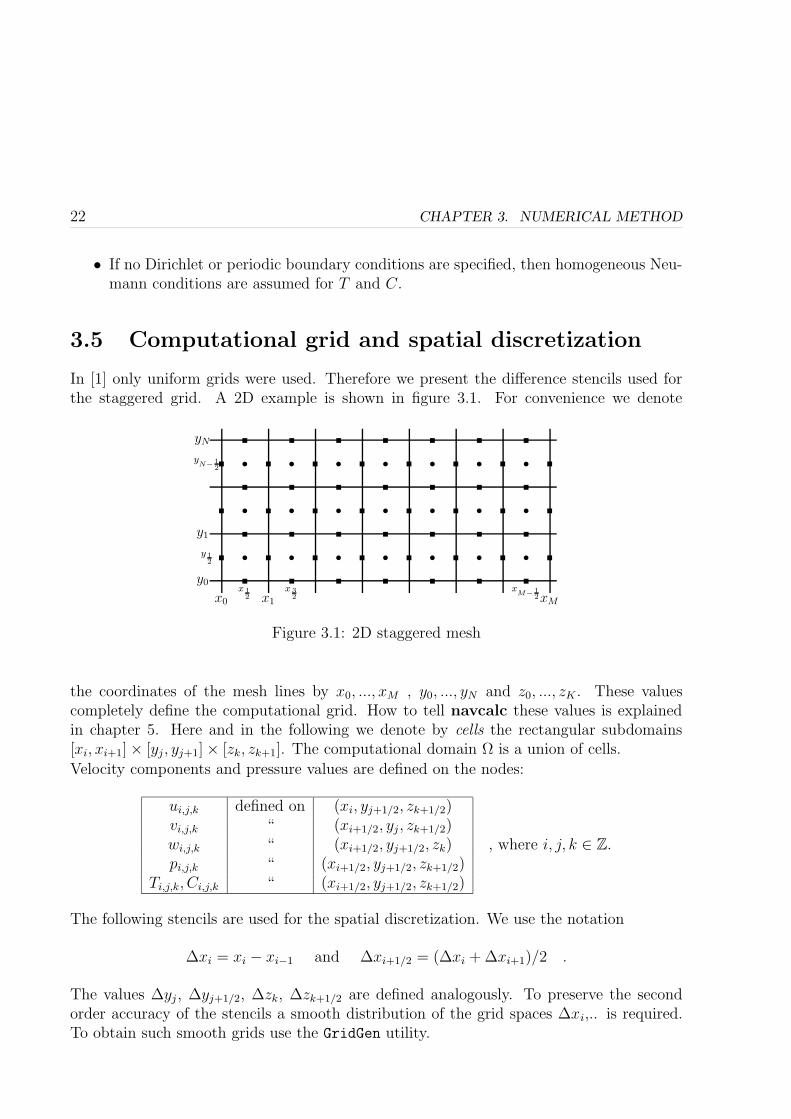
3.5 Computational grid and spatial discretization

In [1] only uniform grids were used. Therefore we present the difference stencils used forthe staggered grid. A 2D example is shown in figure 3.1. For convenience we denote

s s s s s s s

s

s

s

s

s

s

s

s

s

s

s

s

s

s

x0 x1 xM

y0

y1

yN

y 1

2

yN−

1

2

x 1

2

x 3

2

xM−

1

2

Figure 3.1: 2D staggered mesh

the coordinates of the mesh lines by x0, ..., xM , y0, ..., yN and z0, ..., zK . These valuescompletely define the computational grid. How to tell navcalc these values is explainedin chapter 5. Here and in the following we denote by cells the rectangular subdomains[xi, xi+1]× [yj, yj+1]× [zk, zk+1]. The computational domain Ω is a union of cells.

Velocity components and pressure values are defined on the nodes:

ui,j,k defined on (xi, yj+1/2, zk+1/2)vi,j,k “ (xi+1/2, yj, zk+1/2)wi,j,k “ (xi+1/2, yj+1/2, zk)pi,j,k “ (xi+1/2, yj+1/2, zk+1/2)

Ti,j,k, Ci,j,k “ (xi+1/2, yj+1/2, zk+1/2)

, where i, j, k ∈ Z.

The following stencils are used for the spatial discretization. We use the notation

∆xi = xi − xi−1 and ∆xi+1/2 = (∆xi +∆xi+1)/2 .

The values ∆yj, ∆yj+1/2, ∆zk, ∆zk+1/2 are defined analogously. To preserve the secondorder accuracy of the stencils a smooth distribution of the grid spaces ∆xi,.. is required.To obtain such smooth grids use the GridGen utility.

3.5. COMPUTATIONAL GRID AND SPATIAL DISCRETIZATION 23

Diffusive terms:[∂2u

∂x2

]

i,j,k

=1

∆xi+1/2

(ui+1,j,k − ui,j,k

∆xi−

ui,j,k − ui−1,j,k∆xi−1

)

[∂2u

∂y2

]

i,j,k

=1

∆yj

(ui,j+1,k − ui,j,k

∆yj+1/2−

ui,j,k − ui,j−1,k∆yj−1/2

)

The other diffusive terms are discretized in a similar fashion. Stencils similar to the onefor ∂2u

∂y2 are used for ∂2Θ∂x2 ,

∂2Θ∂y2 and ∂2Θ

∂z2 , where Θ is either T or C.

Convective terms:Five different discretizations of the convective terms are possible:

1. Donor-Cell (hybrid-scheme) (1st/2nd order)

2. Quadratic upwind interpolation for convective kinematics (QUICK) (2nd-Order)

3. Hybrid-Linear Parabolic Arppoximation (HLPA) (2nd-Order)

4. Sharp and Monotonic Algorithm for Realistic Transport (SMART) (2nd-Order)

5. Variable-Order Non-Oscillatory Scheme (VONOS) (2nd/3rd-Order) (default)

To select one of these schemes, you have to set the appropriate variable in the scene de-scription file. How to do this is explained in section 5.2. By default the VONOS-scheme isused. In the following the Donor-Cell scheme is briefly described. More details about theother schemes can be found in [3].

Second order convective terms:[∂u2

∂x

]

i,j,k

=(ui+1,j,k + ui,j,k)

2 − (ui,j,k + ui−1,j,k)2

4∆xi+1/2[∂vu

∂y

]

i,j,k

=vi+1/2,j,kui,j+1/2,k − vi+1/2,j−1,kui,j−1/2,k

∆yi

Stencils similar to the one for ∂vu∂y

are used for the discretization of the convective terms in

(3.3) and (3.4), e.g. we have

[∂vT

∂y

]

i,j,k

=vi+1/2,j,kTi,j+1/2,k − vi+1/2,j−1,kTi,j−1/2,k

∆yi.


The unknown values, e.g. vi+1/2,j,k are computed by linear interpolation.

ui,j+1/2,k =∆yjui,j+1,k +∆yj+1ui,j,k

∆yj +∆yj+1

vi+1/2,j,k =∆xivi+1,j,k +∆xi+1vi,j,k

∆xi +∆xi+1

First order upwind:

[∂u2

∂x

]

i,j,k

=kRuR − kLuL

∆xi+1/2, where kR = (ui+1,j,k + ui,j,k)/2 , kL = (ui+1,j,k + ui,j,k)/2

and uR =

ui,j,k : kR > 0ui+1,j,k : kR ≤ 0

; uL =

ui−1,j,k : kL > 0ui,j,k : kL ≤ 0

[∂vu

∂y

]

i,j,k

=kRuR − kLuL

∆yj, where kR = vi+1/2,j,k , kL = vi−1/2,j,k

and uR =

ui,j,k : kR > 0ui,j+1,k : kR ≤ 0

; uL =

ui,j−1,k : kL > 0ui,j,k : kL ≤ 0

Stencils similar to the one for ∂vu∂y

are used for the upwind discretization of the convective

terms in (3.3) and (3.4). First and second order terms can be blended using a parameterα by, e.g.

∂u2

∂x= α(first order) + (1− α)(second order) .

The blending parameter α is user definable (see chapter 5) and may be chosen different forthe equations of momentum and energy or transport of a scalar.

Laplacian for pressure:We employ a conservative discretization which is simply the nested application of thecentered difference for the pressure gradient and the centered difference for the naturaldiscretization of the divergence, e.g.

[∂2p

∂x2

]

i,j,k

=1

∆xi

(pi+1,j,k − pi,j,k

∆xi+1/2−

pi,j,k − pi−1,j,k∆xi−1/2

)

.

Poisson solvers:

For the solution of the linear equation arising from discretization of the pressure poissonequation, the following numerical methods are implemented:

3.6. DISCRETIZATION OF BOUNDARY CONDITIONS 25

1. Successive Overrelaxation (SOR)

2. Symmetric SOR (forward/backward)

3. Red-Black scheme

4. 8-Color SOR

5. 8-Color Symmetric SOR (fw/bw)

6. BiCGStab

To select a method, select the corresponding option in the scene description file(see sec-tion 5.2 on how to do this). By default, the Poisson-equation is solved using the BiCGStab-method.

3.6 Discretization of boundary conditions

As described in [1], Dirichlet conditions for the velocity are implemented by setting thenodal value of the normal velocity component or by linear interpolation for the tangentialvelocity components. The homogeneous boundary Neumann conditions for the pressureare discretized by, e.g.

p0,j,k = −p1,j,k .

In case of convex edges some special treatment is required. Consider the situation shownin Figure 3.2. If Γ1 denotes the face between the cells i,j and i,j+1 and Γ2 the face between

u

u

u u

u u

Obstacle

Fluid

pi,j pi+1,j pi+2,j

pi,j+1 pi+1,j+1 pi+2,j+1Γ1

Γ2

Figure 3.2: convex corner


the cells i,j and i+1,j , then the homogeneous Neumann conditions are discretized by

pi,j = −|Γ1|pi,j+1 + |Γ2|pi+1,j

|Γ1|+ |Γ2|.

Chapter 4

Navcalc and Navcalcmpi

The binary navcalc (or navcalcmpi for parallel computation) is used to run the simu-lation. At the end of a calculation the computed values of u, p, T,C are written in thedata file. The original binary data file is overwritten and can now be used for a restartof a longer calculation or for analysing and postprocessing the computed data. By settinga corresponding option in the scene description file you also have the possibility to savecomputed data in regular intervals. Details on how to specify how often and where thedata is to be stored can be found in section 5.2.

4.1 Command line arguments

The following parameters can be used on the command-line of navcalc:

-h Prints the list of parameters and a short description-b 〈DataFile〉 binary data file. If this option is not given, navcalc

or navcalcmpi try to read the data from a file nameddefault.bin in the current directory.

-t 〈n〉 Sets maximum number of seconds to run. With this optionthe maximum computing time for a specific job can be limited.Default is no restriction.

-p〈n〉 Set info level to n = 0, 1, 2, 3. Depending on the -p argu-ment the amount of additional information that is printed tostdout can be adjusted.

4.2 Parallelization issues

For the parallelization the domain ΩR is divided into several rectangular subdomainsΩ1, . . . ,Ωµ. A simple 2D example is shown in figure 4.1. Each process holds some ghost

27

28 CHAPTER 4. NAVCALC AND NAVCALCMPI

Ω

Ω1 Ω2

Ω3Ω4

Figure 4.1: 2D parallelization example.

cells which overlap inner cells of the adjacent process. Values are copied from these to theghost cells when necessary. To minimize communication, the program divides ΩR in a waythat minimizes the area of the touching faces and equilibrates the number of cells in thedifferent subdomains.The data required for parallelization is kept in the class ParParams which can be found inparallel.hpp. The most important variables are described in the following table:

variable descriptionbiug, biog, bjug,bjog, bkug, bkog

This defines the computational domain for thisprocess (excluding the necessary ghost cells) asbiug, . . . , biog×bjug, . . . , bjog×bkug, . . . , bkog.For your convenience, read access is possible using themacros iug, iog, etc. For example, 1, 16 × 1, 10 ×1, 10 will be divided into 1, 8× 1, 10× 1, 10 and9, 16 × 1, 10 × 1, 10.

me Process ID of this task.tn, ts, tw, te, tb, tt IDs of the neighbour processes in each direction (see fig-

ure 5.2). The value -1 means that there is no neighbourprocess.

4.3 Implementational details

In this section a quick overview of the general structure and the most important aspectsof the implementation are given. For a detailed documentation of the code please refer tothe reference manual.

The main loop of the program reads:

4.3. IMPLEMENTATIONAL DETAILS 29

1 SetObstacleCond(0,0);

2 Par->CommMatrix(U, 1, 0, 0, UCOMM);

3 Par->CommMatrix(V, 0, 1, 0, VCOMM);

4 Par->CommMatrix(W, 0, 0, 1, WCOMM);

5 S.delt=TimeStep();

6 do

7 CompFGH();

8 CompRHS();

9 res=Poisson();

10 AdapUVW();

11 SetObstacleCond(0,0);

12 Par->CommMatrix(U, 1, 0, 0, UCOMM);

13 Par->CommMatrix(V, 0, 1, 0, VCOMM);

14 Par->CommMatrix(W, 0, 0, 1, WCOMM);

15 S.delt=TimeStep();

16 if (S.CompTemp==TRUE)

17 CompTG(T,S.alphatg,S.nu/S.prandtl);

18 Par->CommMatrix(T, 0, 0, 0, TCOMM);

19

20 if (S.CompChem==TRUE)

21 int n;

22 for (n=0; n<S.nchem; n++)

23 CompTG(CH[n],S.alphatg,S.chemc[n]);

24 Par->CommMatrix(CH[n], 0, 0, 0, CHCOMM+n);

25

26

27 S.t+=S.delt;

28 n++;

29 while (S.Tfin < 0);

In lines 1 to 5, a first initialization of boundary values is set and the initial size ∆t of thetime steps is computed. In line 7, u is computed, in the next line 1

∆t∇ · u, see (3). In line

9, equation (3.8) is solved and the new velocity values are computed in line 10 accordingto (3.6). In lines 11 to 14, boundary conditions are set and velocities are exchanged. Fromthe new velocities, the size of the next time step is calculated in line 15 and in line 16 to 26optional transport equations are solved. The following list shows where the most importantclasses can be found.


class fileScene typen.hpp

ParParams parallel.hpp

Navier navier.hpp

NavierCalc navier.hpp

Matrix<T> matrix.hpp

List<T> list.hpp

list objects typen.hpp

Data structures

The physical parameters, information about the grid, precalculated discretizations andsome other stuff is kept in the class Scene. The most important variables are listenedbelow.

variable descriptiongridp[3] This defines the number of cells in every direction for the

whole domain ΩR, the inner cells are numbered from 1to gridp[i], 1 ≤ i ≤ 3. The cells which are computedby the actual process are defined in the class ParParams,which is described in (4.2).

d[3][] This variable contains the spaces between the grid lines inevery direction (see figure 3.1). For convenience: accessis possible using the macros DX[i], DY[j] and DZ[k].

dm[3][] This variable contains the spaces between the middlesof the cells in every direction (marked by the circles infigure 3.1). For convenience: access is possible using themacros DXM[i], DYM[j] and DZM[k].

kabs[3][] This variable contains the absolute positions of the gridlines.

ddstar[3][3][],ddPstar[3][3][],ddSstar[3][3][]

These variables contain different discretizations for thesecond derivative, where the first index selects the direc-tion and the second index selects the appropriate weight(left - 0, middle - 1, right - 2). The discretizations aredescribed in (3.5).

periodbound This is a bit field indicating if periodic boundary con-ditions are set in the appropriate direction (bit 0 - x-direction, bit 1 - y-direction, bit 2 - z-direction).

The 3D matrices, for example velocity and pressure data, are kept in the class Navier.There are two derived classes, NavierSetup and NavierCalc. The dimensions of thesematrices are defined in the following table.

4.3. IMPLEMENTATIONAL DETAILS 31

matrix dimensionflag, P,F, G, H,RHS, T,CH[i]

biug− 1, biog+ 1 × bjug− 1, bjog+ 1 × bkug− 1, bkog+ 1

U biug− 1−µx, biog+ 1 × bjug− 1, bjog+ 1 × bkug− 1, bkog+ 1V biug− 1, biog+ 1 × bjug− 1−µy, bjog+ 1 × bkug− 1, bkog+ 1W biug− 1, biog+ 1 × bjug− 1, bjog+ 1 × bkug− 1−µz, bkog+ 1

The variable µx is set to 1 if periodic boundary conditions are set in x-direction or if thecurrent process has a neighbour in south-direction and 0 otherwise. The variables µy andµz are set in a similar way.The cells where boundary values need to be set (for one specific parallel process) are storedin lists which are defined in NavierCalc.

list containsInflowList cells where Inflow b.c. are set (parameters are stored

in list)SlipList cells where Slip b.c. (Neumann) are set

NoslipList cells where Noslip b.c. (Dirichlet) are setPdpdnList[color][face] cells where prescribed boundary conditions (b.c.) lead

to homogeneous Neumann b.c. for the pressure andwhich have the color color. These cells have exactlyone fluid cell neighbouring at face face.

PSpecdpdnList[color] cells where prescribed boundary conditions (b.c.) leadto homogeneous Neumann b.c. for the pressure andwhich have the color color. These cells have more thanone neighbouring fluid cell. This requires some moreinvolved boundary treatment.

PInOut2List[color][face] cells with the prescribed outflow condition 2, it is as-sumed that no cells with more than one neighbouringfluid cell exist. Some special boundary treatment isrequired.

PInOut1List[color][face] same as PInOut2List for outflow condition 1.

Chapter 5

Navsetup

The main components of the NaSt3DGP package are the two parts navsetup and navcalc.As mentioned before, navsetup produces from a so-called scene description file (*.nav)the so-called data-file (*.bin). The scene description file must contain all information todescribe the flow configuration. This includes the numbers of grid points, the mesh, the ge-ometry of obstacles, place and type of boundary conditions, etc. From this data a compact,internal representation of the flow configuration is computed and written in the data-file.This data-file now contains initial values of the pressure and velocity (p, u), a flag fieldwhich describes the geometry and some general information such as boundary conditionsor physical parameters of the fluid.

The data-file is read by navcalc to run the simulation. After a prescribed number of timesteps and before finishing, navcalc writes the actual pressure, velocity, etc. values in thisfile and thus overwrites the initial data. This new data-file can be used for a restart or forthe analysis of the simulated flow. Since the format of the data-file is rather complicatednavsetup provides the possibility to read a data-file and to write the pressure, velocitycomponents, etc. in separate files which are easier to handle. A simple MatLab V toolwhich reads such files and stores the entries in an 3D array is tools/matlab/ReadNast.m

5.1 Command line arguments

The following is a list of command-line arguments for navsetup:

33

34 CHAPTER 5. NAVSETUP

-h Prints the list of parameters and a short description and prints theversion number of NaSt3DGP.

-s 〈SceneFile〉 Reads the scene description file 〈SceneFile〉 and generates a data-file-b 〈DataFile〉 The name of the data-file, the default name is default.bin-l 〈DataFile〉 load field variables(velocity, pressure etc.) from an existing datafile.

This is useful if you want to run a calculation with previsously com-puted values p, u , T, c, .. but want to change some simulationparameters. You can create a binary file for the new calculation withthe following command:

navsetup -s 〈SceneFileNew〉 -b 〈DataFileNew〉 -l 〈DataFile〉

The data will be interpolated if the number of grid points changes.-L 〈DataFiles〉 Same as -l, but reads several data files 〈DataFiles〉.*.-A 〈TextFiles〉 Same as -L, but reads several text files (written by −a)

〈TextFiles〉.txt.*.-o 〈OutFile〉 This option sets the base of the filename to 〈OutFile〉 for the options

which write files. If this option is not used, 〈OutFile〉 is set to ’default’.-TC 〈DataFile〉 Reads the data p, u , T, c, .. from the data-file and writes to

〈Outfile〉.dat. The file format is ASCII Tecplot. The data written islocated at the cell centers.

-T 〈DataFile〉 same as −TC but writes each field to a separate file named〈Outfile〉.〈field〉.dat, e.g. 〈Outfile〉.u.dat .

-g 〈DataFile〉 Reads the data p, u , T, c, .. from the data-file and writes eachof it in 〈Outfile〉.u, 〈Outfile〉.v etc. These files can be read in Matlabwith the script tools/matlab/ReadNast.m.

-a 〈DataFile〉 Same as −g, but use ASCII-format(text files) which are named〈OutFile〉.txt.*.

-G 〈DataFile〉 Reads the data p, u , T, c, .. from the data-file and writes each ofit in 〈Outfile〉.vtk.u, 〈Outfile〉.vtk.v etc. The files are written in theVTK1 rectilinear grid format.

-GS〈DataFile〉 same as −G but uses the VTK Structured Points format and the filesare named 〈Outfile〉.vtksp.* .

-f uvwptcV create a VTK file including the velocity-field V or multiple scalarsu, v, w, p, t, c0 . . . cN . This option has to be used together with −G,e.g. use the command

navsetup -f V p -G 〈DataFile〉 -o 〈Outfile〉

to write the the velocity as a vectorfield and the pressure p to a filenamed 〈Outfile〉.vtk.mix or use

navsetup -f puv -G 〈DataFile〉 -o 〈Outfile〉

to write the pressure p and the first two velocity components u and v.

5.2. SCENE DESCRIPTION FILE 35

5.2 Scene description file

The scene description file (*.nav-file) is a text-file which is used to specify all necessaryparameters for the calculation. It contains information about the geometry, the mesh, thefluids and is also used to specify initial and boundary conditions. In the following sectionsthe syntax of the scene description file is explained.

5.2.1 Blocks

The scene description file consists of blocks of the form

〈blocktype〉 . . .

where 〈blocktype〉 is one of the keywords

dimension, parameter, box, sphere, cylinder, halfspace, union, intersection,

poly

which are explained below. The blocks are processed in the order as they appear in thefile.

5.2.2 Comments

Comments begin with a double slash followed by a space and end with an end-line charac-ter, for example

// this is a first comment

dimension // this is a comment

. . .

5.2.3 dimension

The dimension block contains information about the grid and the size of the domain Ω.The following keywords are allowed:


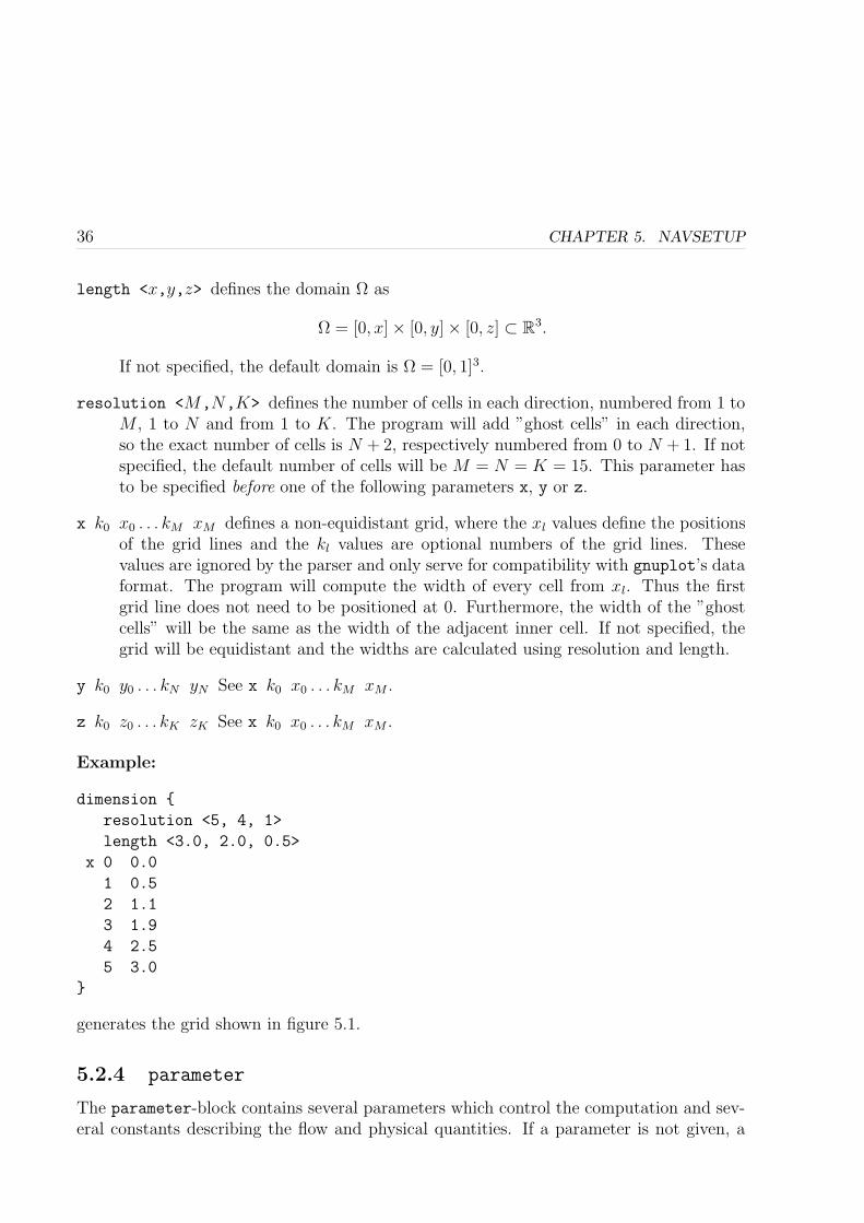
length <x,y,z> defines the domain Ω as

Ω = [0, x]× [0, y]× [0, z] ⊂ R3.

If not specified, the default domain is Ω = [0, 1]3.

resolution <M,N,K> defines the number of cells in each direction, numbered from 1 toM , 1 to N and from 1 to K. The program will add ”ghost cells” in each direction,so the exact number of cells is N + 2, respectively numbered from 0 to N + 1. If notspecified, the default number of cells will be M = N = K = 15. This parameter hasto be specified before one of the following parameters x, y or z.

x k0 x0 . . . kM xM defines a non-equidistant grid, where the xl values define the positionsof the grid lines and the kl values are optional numbers of the grid lines. Thesevalues are ignored by the parser and only serve for compatibility with gnuplot’s dataformat. The program will compute the width of every cell from xl. Thus the firstgrid line does not need to be positioned at 0. Furthermore, the width of the ”ghostcells” will be the same as the width of the adjacent inner cell. If not specified, thegrid will be equidistant and the widths are calculated using resolution and length.

y k0 y0 . . . kN yN See x k0 x0 . . . kM xM .

z k0 z0 . . . kK zK See x k0 x0 . . . kM xM .

Example:

dimension

resolution <5, 4, 1>

length <3.0, 2.0, 0.5>

x 0 0.0

1 0.5

2 1.1

3 1.9

4 2.5

5 3.0

generates the grid shown in figure 5.1.

5.2.4 parameter

The parameter-block contains several parameters which control the computation and sev-eral constants describing the flow and physical quantities. If a parameter is not given, a


-

6y

z

xx0 x1 x5

Figure 5.1: Ghost cells are bounded by thin lines and inner cells are bounded by thick lines.

default value will be used. A complete list of all possible parameters together with anexplanation and the default value is given in table 5.1.All physical quantities, like Dirichlet values for the velocity, temperature or the viscosityare assumed to be given in standard ISO units (m, s, kg, K and derived units), unless thedimensionless-flag is set(see below).

Name Type Default Description

Flow parameters

Tfin double [s] 1.0 defines the (physical) timespan of thesimulation

reynolds double 10.0 is the dimensionless Reynolds-numberwhich describes the ratio between iner-tia and viscous forces in the flow


Name Type Default DescriptionnuC int 0 the paramter nuC sets the number of

species to be transported with the flow.For each species, a diffusion constant hasto be specified in a comma-separated listafter nuC, i.e. the line has to look likenuC nC , ν1, . . . , νnC

where nC is an inte-ger specifying the number of species andνi is a double value which stands for thediffusion parameter of the i-th species.You have to make sure that you alsospecify initial conditions using the key-word cheminit. Details on how to spec-ify initial and boundary conditions aregiven in section 5.2.5

gx double [m/s2] 0.0 x-component of external volume force gin (3.1) (or g0 in (3.9) if the tempera-ture is calculated). In the latter case gis computed from g0 by means of (3.9)

gy double [m/s2] 0.0 Same as gx for the y-componentgz double [m/s2] 0.0 Same as gx for the z-componentfroude double 1.0 the Froude-number is a dimensionless

number describing the ratio between in-ertial and gravitational forces

beta double [1/K] 1e-4 volume expansion coefficient in equa-tion (3.9)

TempRef double [K] 273.0 reference temperature in (3.9)prandtl double 1.0 the Prandtl-number is a dimensionless

number describing the ratio between mo-mentum and heat transfer in the fluid

Timestep control

deltmax double [s] 1.0 upper bound for ∆t


Name Type Default Descriptiontfconv double 0.1 security factor for the timestep restric-

tion arising from the convective terms.In every step, ∆t will be set less or equalthan

∆t ≤ tfconv ·minc∈F

∆xcuc

,∆ycvc

,∆zcwc

where F denotes the set of cells

c = [x, x+∆xc]×[y, y+∆yc]×[z, z+∆zc]

in Ωtfdiff double 0.2 security factor for the timestep-

restriction arising from the diffusiveterms. In every step, ∆t will be set lessor equal than

∆t ≤ tfdiff minν∈N ,c∈F

[

ν( 1

∆xc2+

1

∆yc2+

1

∆zc2

)]−1

and N = ν ∪1/(ν · prandtl)︸︷︷︸

only if temperature

is computed

∪ ν1, . . . , νnC

︸︷︷︸

only if scalars

are computed

.

Data output

prstep int 20 defines when to write the computed val-ues to the binary file. Each prstep-thtimestep the current solution is writtento the binary file(the file is overwritten)

TimePrintStep string - defines an interval (in physical time) af-ter which the solution should be writ-ten to files in a directory specified byTargetDirectory. If TimePrintStep isnot specified, no output will be gener-ated.

TargetDirectory string - specifies the directory(absolut path-name) where the files generated byTimePrintStep should be stored


Name Type Default Description

Parameters controlling numerical methods

TimeDis string EU1 defines the time discretization to beused. Possible values are EU1 for firstorder explicit Euler-Method, AB2 forsecond order explicit Adams-Bashforth-Method, RK2 for second order Runge-Kutta-method and RK3 for third or-der Runge-Kutta-method. Remark: TheRunge-Kutta-method of third order isonly available for the time derivativesin equations (3.3) and (3.4), settingTimeDis to RK3 results in application ofthe Runge-Kutta-method of second or-der to the other time derivatives

ConvectiveTerms string VONOS defines the discretization scheme to beused for the convective terms. Possi-ble values are DC (Donor-Cell, 1st/2ndorder), HLPA (Hybrid Linear-ParabolicApproximation, 1st/2nd order), QUICK(Quadratic Upwind Interpolation forConvective Kinematics, 2nd order),SMART (Sharp And Monotonic Algo-rithm for Realistic Transport, 2nd or-der) and VONOS (Variable-Order Non-Oscillatory Scheme, 2nd order)

PoissonSolver string BiCGStab set the method for solution of the linearsystem arising from discretization of thepressure poisson equation. Possible val-ues are SOR, SSOR, RedBlack, 8Color-SOR, 8ColorSSOR and BiCGStab (pre-conditioned with Jacobi-Method)

alpha double 1.0 defines the blending parameter α in theconvex combination of the central differ-ence/upwind discretization of the con-vective terms of F,G,H. alpha = 1means pure upwind and alpha = 0 re-sults in pure central difference discretiza-tion


Name Type Default DescriptionalphaTC double 1.0 same as alpha, but for convective terms

in the transport equation used for com-putation of temperature and scalars

Parameters for the linear solver

itermax int 100 defines the maximal number of iterationsin the linear solver (BiCGStab,SOR,SSOR etc.)

eps double 0.001 defines the stopping criterion for the it-erations in the linear solver. The param-eter eps is the upper bound for the resid-ual of the poisson equation, i.e. the iter-ations are stopped if

√

1

]F

∑

c∈F

(

∆hpc −1

∆t(∇h · u)c

)2

≤ eps .

Here, F is the set of all fluid cells in Ωand ]F is the cardinality of F . ∆h and∇h denote the discrete Laplacian andgradient operator.

omega double 1.7 sets the relaxation parameter for theSOR-type solvers

Boundary conditions

periodboundx sets periodic boundary conditions in di-rection of x-coordinate

periodboundy same as periodboundx only for the y-coordinate-direction

periodboundz same as periodboundx only for the z-coordinate-direction

Table 5.1: List of entries in the parameter-block


5.2.5 Objects

Objects are used to describe the geometry of the simulation domain and to specify initialand boundary conditions. There are four basic object types, box, sphere, cylinder andhalfspace. Additional geometries and obstacles can be created with the CSG operationsunion, difference and intersection. There exists one restriction for obstacle cells,namely two opposite faces are not allowed to touch fluid cells.As already mentioned in section 5.2.1, objects are just another type of blocks. The com-mands given in table 5.2 can be used inside any object-block.

Name Descriptioncoords <X1,Y1,Z1>,<X2,Y2,Z2> sets the size of box, sphere or cylinder objects to

[X1, X2]× [Y1, Y2]× [Z1, Z2]. The default unit used is onecell. This can be changed by the command absolute

absolute allows use of absolute coordinates given by length

fluid marks the concerning cells as fluid cells. This commandmakes it possible for example to cut quite easily holesinto other objects. fluid can not be defined on ghostcells (e.g. i ∈ 0,M + 1) with non-periodic boundaryconditions in the specific direction

init <u0,v0,w0>,p0 initializes the concerning cells with velocity values(u0, v0, w0) and pressure p0. The default initializationis u0 = v0 = w0 = p0 = 0. These values are not con-cerned as Dirichlet boundary condition

noslip defines the Dirichlet boundary condition u = 0 (see3.4) for the concerning cells. This is the default value.Homogeneous Neumann boundary conditions are setfor temperature and scalars. This is the difference toinflow <0,0,0> (see below) where also u = 0 is set

slip defines Slip boundary condition (see 3.4) for the con-cerning cells

inout n,vΓ defines Outflow boundary condition of type n, 1 ≤ n ≤2, where the additional parameter vΓ is ignored if n = 1.See section 3.4 for an explanation of the different types.If n = 2 and vΓ = 1 the velocity field at the outflowboundaries is corrected to enforce the compatibility con-dition (set vΓ to 0 if you do not want this).

inflow <u0,v0,w0> defines Dirichlet boundary condition u = (u0, v0, w0)(see 3.4) for the concerning cells. When temperatureor scalars are computed, Dirichlet boundary conditionsfor these quantities are set. You must specify the par-ticular values by temperature and/or cheminit


Name Descriptiontemperature Tinit defines Dirichlet boundary conditions on boundary cells

for the temperature Tinit or initializes fluid cells withtemperature Tinit

cheminit c1, . . . , cnCdefines Dirichlet boundary conditions for scalarsc1, . . . , cnC

on boundary cells or initializes fluid cells withthese values

Table 5.2: valid commands inside an object-block

Now we describe the differences between the object-types.

box: The command box defines the box [X1, X2] × [Y1, Y2] × [Z1, Z2] except one of thekeywords north, south, west, east, top or bottom is given. In this case, the box isthe appropriate ”wall” (see figure 5.2):

(0,0,0)

6

-

x

z

y

?

-

6

south

west

top

north

eastbottom

Figure 5.2: wall naming scheme

north M + 1 × 0, .., N + 1 × 0, .., K + 1south 0 × 0, .., N + 1 × 0, .., K + 1west 0, ..,M + 1 × N + 1 × 0, .., K + 1east 0, ..,M + 1 × 0 × 0, .., K + 1top 0, ..,M + 1 × 0, .., N + 1 × K + 1

bottom 0, ..,M + 1 × 0, .., N + 1 × 0

sphere: The command sphere defines the ellipsoid which touches all faces of the box[X1, X2] × [Y1, Y2] × [Z1, Z2] defined by coords. The main axes are parallel to thecoordinate axes.


cylinder: In the same way, cylinder defines a cylinder whose rotation axis is defined byone of the commands x, y or z.

halfspace: The command halfspace defines the set of cells

p ∈ C | axp + byp + czp + d ≥ 0,

where a, b, c, d are given by the command

hesse <a,b,c>,d

and (xp, yp, zp) is the middle of the corresponding cell p.

poly: The command poly defines a polytope bounded by polygons. The points are speci-fied using the command

points n,<a0,b0,c0>,. . . ,<an−1,bn−1,cn−1> .

The first point indexed with 0. After defining points, the polygons have to be bespecified using the command

vertices n,p1,p2,...,pn

where n is the total number of indices (including control indices −1). One polygon isdefined by enumerating the points in clockwise or counterclockwise order, where thefirst point has to be enumerated once again as last point. Then this series is finishedwith index −1. The following example defines a cube:

poly

points 8,<0.0,0.0,0.0>,

<1.0,0.0,0.0>,

<1.0,1.0,0.0>,

<0.0,1.0,0.0>,

<0.0,0.0,1.0>,

<1.0,0.0,1.0>,

<1.0,1.0,1.0>,

<0.0,1.0,1.0>

vertices 36,0,1,2,3,0,-1,

1,5,6,2,1,-1,

4,5,6,7,4,-1,

0,4,7,3,0,-1,

3,2,6,7,3,-1,

0,1,5,4,0,-1


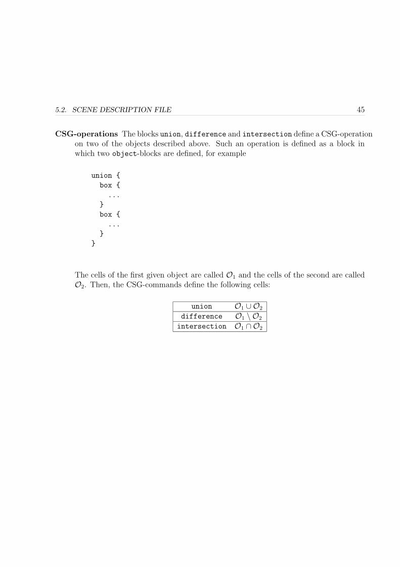
CSG-operations The blocks union, difference and intersection define a CSG-operationon two of the objects described above. Such an operation is defined as a block inwhich two object-blocks are defined, for example

union

box

...

box

...

The cells of the first given object are called O1 and the cells of the second are calledO2. Then, the CSG-commands define the following cells:

union O1 ∪ O2difference O1 \ O2

intersection O1 ∩ O2

Chapter 6

Utilities

In this chapter we give an overview over various useful tools contained in the distributionof NaSt3DGP.

6.1 vrml2nav

The vrml2nav program is a utility to generate mesh and geometry information in the scenedescription file format from a scene given in the VRML 1.0 format1. After installation ofthe NaSt3DGP-package it can be found in the bin directory of the installation path(wherealso navsetup and navcalc reside).

The usage is very simple, just type

vrml2nav 〈vrmlfile.wrl〉

where 〈vrmlfile.wrl〉 is the file containing the description of the scene in VRML 1.0 for-mat. In addition, vrml2nav reads the textfile vrml2nav.cfg. In this file you just need oneline to specify where the output (the scene description in nav-format) should be written.The line begins with the keyword outputnav followed by a filename, i.e.

outputnav 〈outfile.nav〉

This procedure generates a scene description file which can be processed with navsetup asdescribed in chapter 5 to generate an input file for the calculation. The vrml2nav utilitywrites some default values for the different parameters like Reynolds-number etc. in thenav-file. These parameters as well as the grid resolution should be adjusted according tothe calculation to be done. The nav-file generated by vrml2nav can be edited with any

1Virtual Reality Modelling Language, see http://www.web3d.org/technicalinfo/specifications/VRML1.0/

47

48 CHAPTER 6. UTILITIES

text-editor and all parameter settings explained in section 5.2 can be used. The poly-blocksin the scene description represent the actual geometry given in the VRML 1.0 file.

Figure 6.1: Snapshot of a Porsche model, VRML 1.0 scene (top), Tecplot visualization offlag field(bottom)

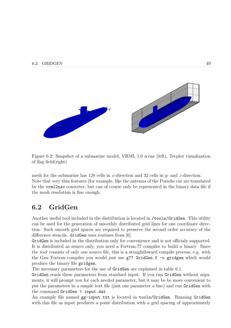
In figures 6.1 and 6.2 two examples are given. On the left a screenshot of the original VRML1.0 description is shown, on the right side a visualization of the corresponding translationinto the nav-format is shown. The visualization was done with Tecplot in the followingway: first the binary data file was generated with navsetup, then, also with navsetup,output for Tecplot was generated (see chapter 5) and within Tecplot the isovalue 1.0 of thevariable flg (which stands for flag field) is visualized. For the Porsche, a mesh resolutionof 180 cells in x-direction, 90 cells in y-direction and 120 cells in z-direction was used, the

6.2. GRIDGEN 49

Figure 6.2: Snapshot of a submarine model, VRML 1.0 scene (left), Tecplot visualizationof flag field(right)

mesh for the submarine has 128 cells in x-direction and 32 cells in y- and z-direction.Note that very thin features (for example, like the antenna of the Porsche car are translatedby the vrml2nav converter, but can of course only be represented in the binary data file ifthe mesh resolution is fine enough.

6.2 GridGen

Another useful tool included in the distribution is located in /tools/GridGen. This utilitycan be used for the generation of smoothly distributed grid lines for one coordinate direc-tion. Such smooth grid spaces are required to preserve the second order accuracy of thedifference stencils. GridGen uses routines from [6].GridGen is included in the distribution only for convenience and is not officialy supported.It is distributed as source only, you need a Fortran-77 compiler to build a binary. Sincethe tool consists of only one source file, this is a straightfoward compile process, e.g. withthe Gnu Fortran compiler you would just use g77 GridGen.f -o gridgen which wouldproduce the binary file gridgen.The necessary parameters for the use of GridGen are explained in table 6.1.GridGen reads these parameters from standard input. If you run GridGen without argu-ments, it will prompt you for each needed parameter, but it may be be more convenient toput the parameters in a simple text file (just one parameter a line) and run GridGen withthe command GridGen < input.dat.An example file named gg-input.txt is located in tools/GridGen. Running GridGen

with this file as input produces a point distribution with a grid spacing of approximately


Table 6.1: Necessary parameters for GridGenvalue type descriptionL int number of locations where grid spaces should take prescribed

valuesx0 float locations in increasing order:xLdx0 float prescribed grid spaces at locations x0...xL:

dxLK int number of grid lines, which should have exactly some pre-

scribed coordinatesxe0 float locations in increasing order: Note, xe0==x0 and xeK==xL are required

xeK This feature allows to generate meshes, which respect somegeometrical constraints

fak float the grid spaces dx0,..dxL can be multiplied with fak. Thisallows a simple coarsening / refinement of the computationalgrid

”workdir” string a directory in which the output files should be written

.01295 at the boundary points 0 and 1 and a spacing of approximately 0.0518 around themidpoint.

The results of GridGen are written to the following files:

gridpoints.gnu contains a numbered list of the gridpoints which can then be usedin a scene description file (see section 5.2)

gridspaces.gnu this file contains the distribution of grid spacesBoth files can be plotted by gnuplot to control the results.

6.3 Interface to MatLab

MatLab is an extremely powerful software package that is very useful for post- and prepro-cessing as well as analysing the computed data in detail. Therefore we include two MatLab-scripts in the NaSt3DGP-package. These scripts, ReadNaSt3D.m and WriteNaSt3D.m, canbe used within Matlab to read or write data in the format that navsetup produces whenusing the -g switch. The format of these files is shown in table 6.2.

After installation of the NaSt3DGP-package, the MatLab-scripts can be found in tools/matlab.

6.4. INTERFACE TO VTK 51

type count descriptionint 3 Number of cells (M,N,K) in each direction (including ghost cells)

float M Coordinates of grid lines in x-directionfloat N Coordinates of grid lines in y-directionfloat K Coordinates of grid lines in z-directionfloat M ·N ·K Data of the corresponding field

Table 6.2: file format generated by navsetup -g

6.4 Interface to VTK

The Visualization Toolkit (VTK) is a freely available2 software package for visualization, 3Dcomputer graphics and image processing. It consists of a C++ class library and interfacesto several scripting languages such as Python or Tcl/Tk.

For visualization of NaSt3DGP-generated data with VTK we have included the scriptviewNaSt3DGP.tcl in the package. It uses the Tcl/Tk bindings of VTK to provide aneasy-to-use GUI to control the displayed data. The script requires a proper installation ofVTK (release 4.0 or newer), compiled with support for the Tcl/Tk bindings.

After installation of NaSt3DGP the script can be found in tools/visualization/vtk/.

To visualize data using viewNaSt3DGP.tcl first create files in VTK-readable format usingnavsetup with the -G and -o 〈datafile〉 switch (this will create the files 〈datafile〉.vtk.p,〈datafile〉.vtk.u, 〈datafile〉.vtk.v and so on, see section 5.1 for details). While converting thedata navsetup will produce output which contains a passage similar to that in table 6.3.

Table 6.3: Sample output of navsetup while converting data.

Writing data.vtk.fl...

Writing data.vtk.u...

u: min -1.70416e-07 max 1.70436e-07

Writing data.vtk.v...

v: min -2.58760e-07 max 2.16669e-07

Writing data.vtk.w...

w: min -3.55411e-09 max 3.55600e-09

Writing data.vtk.p...

p: min -3.02805e-01 max 3.02544e-01

Writing data.vtk.t...

t: min 2.92460e+02 max 2.93542e+02

2see http://public.kitware.com/VTK/ for further information and download


Now you may use the command vtk viewNaSt3DGP.tcl 〈datafile〉 to start the Tk-based GUI (depending on the locations of your datafiles and viewNaSt3DGP.tcl you mayhave to supply appropriate paths to the above command). This will produce two windowson your screen (see figure 6.4), the Tk-based GUI and the window into which VTK rendersits output. Initially the render window will only show the bounding box of the data set(you can turn the bounding box on and off by clicking the button labeled “Frame”).

Figure 6.3: The VTK render window and the viewNaSt3DGP GUI

Inside of the render window you can use the buttons of your mouse to rotate (left button),move (middle button/both buttons) and zoom (right button) the displayed object. Thebutton labeled “Exit” of course ends the application. Clicking the button “ppm” willexport the current content of the render window to a ppm file, the files will be namedsnapshot 1.ppm, snapshot 2.ppm and so on (Note, however, that the window content isnot rendered off-screen, so e.g. overlapping windows or the mouse-pointer would also beexported to the ppm-file).You can now add selected data using the two pulldown-menus on the top right of the GUIwindow. The menus “Slice” and “IsoSurf” are used to set the field variable which is to bedisplayed either on cut-planes (slices) or on an isosurface, respectively. In the entry field“IsoSurfValue” you have to enter the value for which the isosurface should be computed.With the button labeled “On/Off” you can toggle the isosurface. The two sliders are usedto control the opacity of the isosurface and the displayed flag field (if there are obstaclesin your data file). With the remaining buttons you can toggle the visibility of the cut-planes or move them through the domain. To adjust the color palette to the range of thedisplayed variable simply enter the appropriate maximum and minimum values into thecorrespondingly labeled fields.

Chapter 7

Examples

In this chapter we present some examples of calculations done with the NaSt3DGP-package.The scene description files for these and some other testcases are included in the distributionand can be found under the examples-directory.

7.1 Lid-driven cavity

A basic scene description file for the lid-driven cavity problem can be found in the examplesdirectory in the subdirectory Cavity2D (this file was also used in the introductory chapter).For this calculation some parameters have to be adjusted. These benchmark results referto the cavity flow at Re = 1000. For the convective terms, the 2nd/3rd order VONOSscheme was used. Calculations are done on a 48x48 grid and a 96x96 grid. The Poissonsolver is stopped when Res< 1e− 8.

All test computations were finished after 300 time units. The level-values for the stream-function/vorticity are taken from [4].

53

54 CHAPTER 7. EXAMPLES

Fig.6: Vorticity, 48x48 grid Fig.7: Vorticity, 96x96 grid

Fig.8: Streamfunction, 48x48 grid Fig.9: Streamfunction, 96x96 grid

7.1. LID-DRIVEN CAVITY 55

−0.4 −0.2 0 0.2 0.4 0.6 0.8 10

0.2

0.4

0.6

0.8

1

−0.4 −0.2 0 0.2 0.4 0.6 0.8 10

0.2

0.4

0.6

0.8

1

Fig.10: U-values through the vertically Fig.11: U-values through the verticallygeometric center, 48x48 grid geometric center, 96x96 grid

0 0.2 0.4 0.6 0.8 0.9 1

−0.4

−0.2

0

0.2

0.4

0 0.2 0.4 0.6 0.8 0.9 1

−0.4

−0.2

0

0.2

0.4

Fig.12: V-values through the horizontal Fig.13: V-values through the horizontalgeometric center, 48x48 grid geometric center, 96x96 grid

56 CHAPTER 7. EXAMPLES

Chapter 8

In case of Trouble

8.1 Submitting bug reports

If you obtain any compile or runtime errors please report the bug via email [email protected] simplify our handling of error reports please include the following information

• The version of NaSt3DGP.

• In case of build problems: the output of the make/compile process

• In case of runtime errors: the output of navsetup, navcalc or navcalcmpi.

• A detailed description of machine and operating system.

• The scene description file.

Please send reports about more than one problem in separate messages.

57

58 CHAPTER 8. IN CASE OF TROUBLE

Chapter 9

License

Following is the license under which the software package NaSt3DGP is distributed. Thislicense is also contained in the file COPYING included in the distribution.

License Agreement for the Software Package NaSt3DGP

between the Institut fur Angewandte Mathematik der Rheinischen Friedrich-Wilhelms Uni-versitat Bonn - hereinafter referred as licenser - and You - hereinafter referred as licensee.

§1 Object of Agreement

The licenser lets to the licensee the right of the temporarily unrestricted use of the softwarepackage NaSt3DGP.

§2 Property and Copyright

The licenser is the owner of all rights of NaSt3DGP including all contributions made byothers. We do this to make the code freely available on one hand, and on the otherhand, to synchronize and steer the further development. Of course we appreciate andacknowledge the contributions of others by maintaing the ”Thanks” section. You can alsoadd ’Programmed by ...’ comments in the code that you contribute. If this is unacceptablefor you, then don’t contribute code.The licensee agrees to publish scientific results obtained with NaSt3DGP with an appro-priate citation of the licenser. Details for appropriate citation are stated in the next section.

§3 Appropriate Citation

The licensee agrees that any reports or published results obtained with the SoftwareNaSt3DGP will acknowledge its use by the appropriate citation of the licenser as follows:

59

60 CHAPTER 9. LICENSE

“NaSt3DGP was developed by the research group in the Division of Scientific Computingand Numerical Simulation at the University of Bonn.”Any published work which utilizes NaSt3DGP shall include the following references:1. M. Griebel, T. Dornseifer and T. Neunhoeffer, Numerical Simulation in Fluid Dynamics,a Practical Introduction, SIAM, Philadelphia,(1998)

§4 Obligations of the Licensee

It is in the licensees responsibility that all employees and students with access to NaSt3DGPfollow the restrictions of this agreement.It is not permitted to sell NaSt3DGP or parts of it or results obtained with it. Furthermore,it is not allowed to use NaSt3DGP for any commercial purposes.Any modifications or extensions made by the licensee fall under these stipulations.

§5 Liability

NaSt3DGP is an experimental code. The licenser does not guarantee that NaSt3DGP iserror free and that it complies to the special requirements of the licensee. The licenser doesnot assume any liability.

§6 Supplementary Provisions

The agreement shall be governed and construed in accordance with German law. The placeof jurisdiction is Bonn/Germany.

Bibliography

[1] M. Griebel, T. Dornseifer and T. Neunhoeffer Numerical Simulation in Fluid Dynam-

ics, a Practical Introduction, SIAM, Philadelphia,(1998)[2] J.G. Heywood, R. Rannacher and S. Turek Artificial Boundaries and Flux and Pressure

Conditions for the Incompressible Navier Stokes Equations

[3] V.G. Ferreira, M.F. Tome, N. Mangiavacchi, A.O. Fortuna, A.F. Castello, J.A. Cumi-nato, S. McKee High Order Upwinding and the Hydraulic Jump

[4] O.Botella and R. Peyret Benchmark Spectral Results on the Lid-Driven Cavity Flow,

Computers & Fluids Vol. No. 4 pp. 421-433, 1998[5] Croce Ein paralleler, dreidimensionaler Navier-Stokes Loser fur inkompressible

Zweiphasenstromungen mit Oberflachenspannung, Hindernissen und dynamischen

Kontaktflachen, Masters Thesis, University of Bonn, 2002[6] W.H. Press, S.A. Teukolsky, W.T. Vetterling and B.P. Flannery Numerical Recipes in

Fortran: the Art of Scientific Computing, Cambridge University Press, 1986

61

NaSt3DGP - Research Group Prof. Griebelwissrech.ins.uni-bonn.de/research/projects/NaSt3DGP/... ·...

Documents

Transcript of NaSt3DGP - Research Group Prof. Griebelwissrech.ins.uni-bonn.de/research/projects/NaSt3DGP/... ·...