' NASA TECHNICAL NASATMX.39sz _-

MEMORANDUM

,,,.4U'IO_re')

|

I,,-O

PREDICTION OF THE ACOUSTICm:

_ IMPEDANCE OF DUCT LINERS

By

William E. Zorumski and Brian J. Tester* 1

"-Y :;]

September 1976 i,:' SEP1976 ,RECEIVED _.,

•" _. _ASASln _ClUTY ,_ •IHPIITBRANCH--

, ¢

]

This IJlformal documentation medium is used to provide accelerated or

special release of technical Information to selected users. The contentsmay not meet NASA formal editing and publication standards, may be re-vised, or may be incorporated in another publication.

t

" NATIONALAERONAUTICSANDSPACEADMINISTRATIONID

LANGLEYRESEARCHCENTER,.HAMPTON,VIRGINIA23665

(HASA-TM-X-73951) PRBDTCTIOH OF THE H76-31979ACOUSTIC IH?EDAHCE OF DUCT LINERS (HASA)

65 p HC $4 50 CSCL 20A• Unclas

G3/71 02_. _]

............................... ,_ ......_

1976024891

-4i: i i "_

f

!i !

• i

,_ : I. Report No. _ 2. Government/_ No. 3. RecilJns's _talo g No.

' NASA TM X-73951 I_ 4. Title end ,_bSitle 6. Report Date

, Prediction of the Acoustic Impedance of September 1976Duct Liners e. Pe'fo,'mingo,_,;,at_®code

• 2_1Q ,,7. Author(s) 6. Performing Organization Report No

William E. Zorumski and Brian J. Tester*

10. Work Unit No.

e. _for_l_ 0r_nlatlonN,meml _m 5 0 5- 0 3- 21- 01 i 1NASA Langley Research Center .. ContractorGrantNo.

• I

Hampton, VA 23665 ,'i13.TV_ ofR_ andPeriodCOv_ I

12.Stalin0_v _m and_,_ Technical Memorandum ;i

National Aeronautics and Space Administratiot 14.S_n_i_ Age.cvCodeWashington, DC 20546 ]

15. Supplementary Notes _ _

*Consultant _!

16. Abstract !ii

acoustic impedance of duct liners is reviewed. This review

includes the linear and nonlinear properties of sheet and bulk

type materials and methods for the measurement of these properties.

It also includes the effect of grazing flow on the acoustic

properties of materials. Methods for predicting the propertiesof single or multilayered, point reacting or extended reaction, 1and flat or curved liners are discussed. Based on this review, ' _i

methods for predicting the properties of the duct liners which ']are typically used in aircraft engines are recommended. Some I

areas of needed research are discussed briefly. :i

I

i1!

,1

........... 't17. Keywo,_ (su_ea hv Auti_,ls)J ISTARcat_ u,der.._)' SO.D_.,l_tl_ _ ........ .]

Duet Liners, Acoustic Impedance Unclassified ,jNoise Prediction

Unlimited ]I

19. Security Cla,:if. (of thle reWt) 20. Security Cl|lslf. (of this page) 21. No. of Page,s 2_. I_ice" i

Uncla_,_ified Unclassified 53 :.. $4.25 _

_The Natlot_il Technical Information Service, Springfield, Virginia 22151"Available from ]! STIF/NASA Scientific and Technical Information Facility, P.O. 0ox 33. College Perk. kid 20740

°:'_'_°'"__i°:°°"_ " '*'°:°'""°' ....... i"S_/5-_*±:024891"....-TsA03_ °

CONTENTS

Section 1 INTRODUCTION 1

Section Z ACOUSTIC .MATERIALS 3

2. 1 Linear Impedance 42.1. i Sheet Materials 42. I.2 Bulk Materials 6Z. I.3 Measurement Methods 7

Z. 2 Nonlinear Impedance of Thin Sheets 11Z. Z. 1 Perforated Sheets 14

.- 2.2. Z Uniform Porous Materials 162.2.3 Measurement Methods 17

Z. Z.4 Linearization of Impedance 19Z. 3 The Effect of Grazing Flow 21

2.3.1 Empirical Models 2iZ.3.Z Measurement Methods 25

" Z.4 Recommended Methods for Materials 29

• Section 3 DUCT LINERS 33

3. 1 Flat Point Reacting Liners 333.2 Flat Extended Reaction Liners 353.3 Recommended Methods for Liners 36

3.4 Example Liner 38

Sec tion 4 RECOMMENDED PREDIC TION ME THODS 39

4. I Single-Layer Liner Configurations 394.2 Multilayer Configurations 43

Section 5 CONCLUDING REMARKS 49

Section 6 REFERENCES 51

_ °

3

Jy.

1976024891-TSA04

b •

ABSTRACT

Recent research which contributes to the prediction of the acoustic impedance

of duct liners is reviewed. This review includes the linear and nonlinear

properties of sheet and bulk type materials and methods for the measurement

of these properties. It also includes the effect of grazing flow on the

acoustic properties of materials. Methods for predicting the properties of

single or multilayereda point reacting or extended reaction, and fiat or

curved liners are discussed. Based on this review, methods for predicting ,

the properties of the duct liners which are typically used in aircraft engines

are recommended. Some areas of needed research are discussed briefly.

i_ii iii

1976024891-TSA05

S UMMA R Y

The methods of predicting the acousLic properties of duct liners is reviewed.

The review is divided into a discussion of typical acoustic materials and a 1 i

: discussion of methods of predicting the liner properties from these material !i

• properties. Acoustic materials are usually described by their acoustic

:_ impedance. For thin sheets of materials, this impedance relates the pres-

' sure differential across the material to the velocity through the material. _

For bulk materials, the impedance relates the pressure gradient to the

__ velocity. There are two commonly used methods of measuring impedance.

These are the standing wave method and the two microphone method. ACoustic

materials exhibit significant amounts of nonlinear behavior at the high inten-

sities usually found in aircraft engine ducts; however, this nonlinearity iS

well described by the measured flow resistance of the material. Also,

• _ tangential flow has a large effect on material properties. The best available

information indicates that these effects can be accounted for by the material-j

flow resistance in the presence o£tangentialilow. In most practical problems,

it is necessary to linerize the material properties by use of an rms velocity

in the material, however, this velocity must be found by an iteration procedure.

Bulk materials can be characterized by two measured parameters, the imped-

ance and wave number. The properties of complex duct liner configurations

are predictable once the liner material acoustic properties are knOwn.

v/

MCDONNELL DOUGL_

1976024891-TSA06

I

SYMBOLS

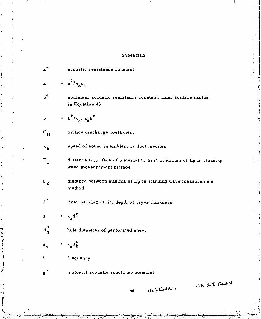
$a acoustic resistance constant

• na = a /PaCa /i

b"' nonlinear acoustic resistance constant; liner surface radius

in Equation 46 i

• b eb = b /Pa; ka

[

i

C D orifice discharge coefficient

• c a speed of sound in ambient or duct medium

i

' D 1 distance from face of material to first minimum of Lp in standingwave measurement method

D 2 distance between minima of Lp in standing wave measurement?

method

d::" liner backing cavity depth or layer thickness

d = kad* i

i

.,_ d_n hole diameter of perforated sheet

l *dh = kad h

f frequency

g material acoustic reactance constant

]97602489]-TSA07

AI.,_, _ - g /PaC_k

( , nonlinear material, acoustic reactance constant

qr b = h ]Pa

I

K grazing flow constant

k* wave number

k = k /ka

k a = _/c a

k_ complex wave number constant for bulk materials

k wave number in extended reaction Liners

k acoustic mode axial wave number in ductzm

L standing wave ratio, dB

Lp sou_.d pressure level, dB re 2 x 10 -5 N/m 2

F thickness of porous or perforated sheet material

M Mach number of mean tangential, grazing or duct flow4

M_0 material acoustic inertance

viii

1976024891-TSA08

; I

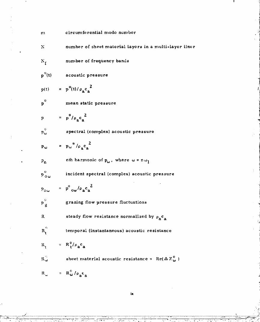
m circumferential mode number

i:

N number of sheet material layers in a multi-layer liner

Nf number of frequency bands

p':_(t) acoustic pressure

?Z

p(t) = p*(t)/OaC a 'i1

p mean static pressure ]1

1• z

p = p /PaCa

Pw spectral (complex) acoustic pressure

Z* c

P_ = P_ /Pa a

• Pn nth harmonic of P¢o, where ¢o = n_o1

Pow::' incident spectral (complex) acoustic pressure

ZPoe = P""ow /PaCa 1

p g grazing flow pressure fluctuations _

R steady flow resistance normalized by PaCa

R t temporal (instantaneous) acoustic resistance

R t = R'/p ct _ a

R,o sheet material acoustic resistance = Re(/XZw )

R: = R w/PaCa

vJ

ix

.1" 4 '_

1976024891-TSA09

R n sheet material specific acoustic resistance at nth harmonic _ = ::.,

R e sheet material specific acoustic resistance based on steady flo_vresistance, R

I

Rh::, specific orifice or hole acoustic resistance ir effective honeycomb cell radius

° i tI

t time iiI

):c it = tot

U"" mean tangential, grazing or duct flow velocity

v(t) acoustic particle velocity normalized by c a

v steady-flow Mach nurnber normal to liner

v spectral (complex) acoustic particle velocityi_" (.U

!

V W : V i.O/C a.

Vn nt:h harmonic of vu_ where _ = nw l

ib

v e total effective particle velocity

X t temporal (instantaneous} acoustic reactance

., Xt = torXt/Oaca

'_',. X[_ sheet material acoustic reactance ----Ira( A Z_ )i'

. i

_:' X:i;. X_ = / PaCa

sheet material specific acoustic reactance at nth harmonic n_ 1. ; X n

_I: X measured and/or calculated sheet materiat specific acoustic

C

reactance

x axial coordinate in standing wave tube

X/

! o)

1976024891-TSA10

,t I

I' !t

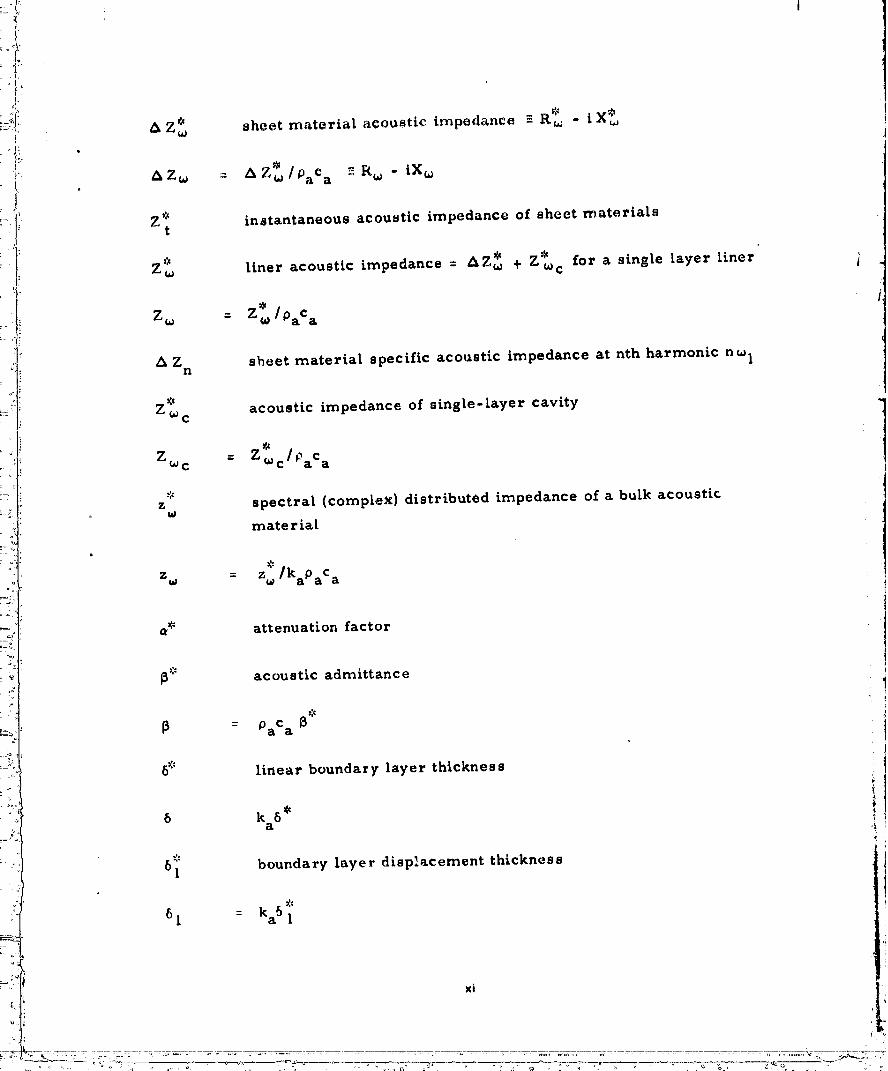
.... i_ _ Z_ sheet material acoustic impedance _ R_ - i _:'_

.t' . AZw _ AZ_/OaC a _ R w - iX w

_/Ii: Z':' instantaneous acoustic impedance of sheet materials_t

*:_ Z w liner acoustic impedance = AZ_ + Z _c for a single layer liner i

Z_o = Z_o/PaC a

A Zn sheet material specific acoustic impedance at nth harmonic noJ 1

Z_'_ acoustic impedance of single-layer cavityC

/ OaC aZwc = Zo_ c

z spectral (complex) distributed impedance of a bulk acoustict_

material

a

z w = zw/kaPaCa

a _" attenuation factor

fl_:: acoustic admittance

6":: linear boundary layer thickness

G k5a

5"_ boundary layer disp_.acement thickness

5I : ka5 I

i

k oound wavelength

v kinematic viscosity

Oa density of ambient medium

Oe sheet material effective density I

open area of perforated sheet, porosity of material

c _rCular frequency

fundamental frequencye l

_, reference frequencyr

Subscripts

i denotes frequency band i (in place of _a,

+ refers to steady flow suction normal to the liner

(i.e., from duct into liner)

- refers to steady flow blowing normal so the liner

(i. e., from liner into duct)

Suot" r script s

{nt refers to nth lay_ r in a multilayer liner

.q,

denotes a dimensional quantity; exceptions are the common

symbols c a , k a, k. Pa' w.

xli

2

]g7602489]-TSA]2

, [ .

1

Operatore t• _ .!

Re, !rn real, imaginary part of j

A difference in a quantity ii

gradient vector i

,!z )jV divergence (gradient) or Laplacian _

• ti ,

O/8t partial differentiation with respect to time, t iF

Z t: temporal (instantaneous) impedance operator

* + * _'et*/R t X t

Zt - Rt+ Xt e/at

q

i:_ '.

,1_.li i

._ ',

ill) _

_-;

:?! ""' 1i .

, oO : o , 0_. /1 . o ..........

1976024891-TSA13

I: lt

Section !

IN T RODUC TION

Duct liners are used to reduce noise in a number of s_tua_Aons. One

application for duct liners is the nacelles of r,_,odern aircraft engines. In

. this environment, the liners are exposed to high-intensity sound, (Refs. !,

Z, 3}, high-speed flow, and large temperature variations_ B,cause _::,fnon-

acoustical requirements, only a few materials have ever been quali.:_c'_for

service in aircraft engines. A perforated sheet _._one material "_.,,_'c!_has

been used, porous metals and rigid fiberglass sheets ,.....Jth,_...o

One goal of aircraft noise research is to dew:lop the abilityto predict the

acoustical performance of new nacelle duct treatments. This prediction

abilitymust be based on the properties of duct liners;hence, the present

paper considers the scbproblem of predicting the properties of duct liners.

• In any prediction scheme, experimental data must be included at some point,

for example, the stiffnessof a structure is predicted from the experinaental

i'. knowledge of the modulus of elastici;y from which the structure is made.

Thus, part of any_-rediction scheme is the identification of those properties

which are to oe measured.

This report reviews the state of knowledge of the properties of acoustic

materials and the way these properties are measured. The physical

variables which affect the acoustical properties of materialJ are discussed

and measurement methods are recommended which account for the presence

of the most important physical effects. Then, methods for predicting the

acoustical properties of complex duct liner configurations are given.

I

Section Z

ACOUSTIC MATERIALS

d

The propagation and attenuation of sound in lined flow ducts is understood in

physical terms such that a mathematical description fallsnaturally into two

_arts. One is generally concerned with how sound that is generated within

the duct propagates through the duct floW fieldand out through the duct term- :1

ination into the far field,while the other is centered on the absorption of I

sound by the duct boundaries. Both areas have been studied intensively

although the former has attracted more attentionrecently since ithas been

realized that the sound radiation can be sensitive to mean flow conditions

within and exterior to the duct even when dissipation processes within the

flow are ignored. The absorption or dissipation of acoustic energy by the

lined duct surfaces is historicallya well established subject, but it has been6

known for some time that in the present context the classical models of

sound absorption must be considerably modified to take i.ltoaccount high-

intensitysound and grazing flow effects.

In this section ",.'eare concerned with the way in which the physical process

of sound absorption by an acoustic material is described throagh the imped- :

ance concept. In general this concept aliows us to link the absorption and

propagation processes without the need to c_nsider how sound absorption is

related to the physical properties of the liner materials (e.g., porosity,

surface density, fiber size). That is then a separate problem which is

outside the scope of the present effort, but nevertheless is one of consider-

able importance. We also review the largely empirical methods which3

attempt to represent the observed influence of sound intensity and grazing

flow on the sound absorption processes through a modification of the imped-

ance parameter. In a sense these real effects affect the convenient division

t of the mathematical description into two parts; that is, in practice, the... absorption process cannot be specified until the local sound field is known

but this depends on the propagation processes {as well as the local sound

field) so that one process depends upon the other.

a . NOT l ILIEV

1976024891-TSB01

1

' I

: !i

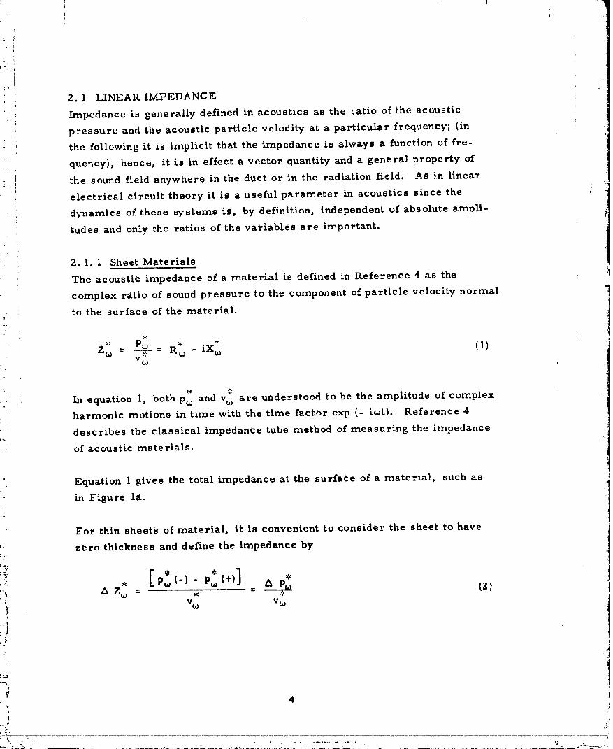
2. l LINEAR IMPEDANCE

Impedance is generally defined in acoustics as the ".atio of the acoustic

pressure and the acoustic particle velocity at a particular frequency; (in

the following it is implicit that the impedance is always a function of fre-

quency), hence, it is in effect a vector quantity and a general property of

; the sound field anywhere in the duct or in the radiation field. A_ in linear

electrical circuit theory it is a useful parameter in acoustics since the

dynamics of these systems is, by definition, independent of absolute ampli-

tudes and only the ratios of the variables are important.

;= 2. 1. I Sheet Materials

The acoustic impedance of a material is defined in ReferenCe 4 as the

complex ratio of sound pressure to the component of particle velocity normal

to the surface of the material.

_',." P_ * . *Z_ = _ = R e -lX_ (1)

In equation 1, both p_ and v_ are understood to be the amplitude of complex

harmonic motions in time with the time factor exp (- i_t). Reference 4

describes the classical impedance tube method of measuring the impedance

of acoustic materials.

Equation 1 gives the total impedance at the surface of a material, such as

in Figure Is.

For thin sheets of material, it is convenient to consider the sheet to have

zero thickness and define the impedance by

[, • ]"'_" P_(') " P_(+) _ A *

I VLO V_

4

1

1976024891-TSB02

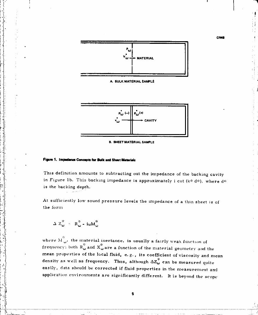
B. SHEET MATERIAL SAMPLE

_, Fiilum t. Imlmdmme Con_ptt for Ekalt _ Shlet Matmids

This definition amounts to subtracting out the impedance of the backing cavity

in Figure lb. This backing impedance is approximately i cot (k::-"d".-'), where d':'

is the backing depth.

At sufficiently low sound pressure levels the impedance of a thin sheet is of

the form

,X Z_ :: R_- i_oM_o

where .Xl w, tile material inertance, is usually a fairly weak function of

frequency; both R_and X ":c• _are a function of the material geometry and the

mean properties of the local fluid, e. g., its coefficient of viscosity and mean,r

density as well as frequency. Thus, although AZt_ can be measured quite

easily, data should be corrected if fluid properties in the measurement and

application environments are significantly different. It is beyond the scope

5

1976024891-TSB03

of the present report to review the functional dependence of AZ_ on the

material geometry and the fluid's mean properties although it is given when

we consider the special case of perforate materials below since it is of a

particularly simple form.

2. 1.2 Bulk Materials

Scott (Reference 5) has shown that the propagation of sound waves in isod

tropic porous materials can be characterized by two complex constants.

Scott used a complex wave number and density; however, other pairs of

constants may be used also. For example, Bies (Reference 6, ch. 10) uses

a complex propagation constant and characteristic impedance to characterize

bulk materials.

In this report, we will use a distributed impedance, or impedance per unit

length, to relate the pressure gradient to the velocity in an i_otropic porousmedium.

V Pco + zcov_o = 0 (3)

The form of equation 3 is used here because of the analogy to equation 2.

The gradient of pressure is approximated by - A pco/l where _ is the

thickness of a thin sample such as in Figure lb. Equation 3, together with

the wave equation given by Scott (Reference 5).

V2 Pco + kco Pco = 0 (4)

completely describe the properties of waves in infinite media, porous or

otherwise. In the limit of 100 percent porosity the porous medium is the

ambient medium and then

kw : w/c a (5)

1976024891-TSB04

_* T l 1

which is a real number, andi ,

i" . z w - .i_oa (6)

i

> which is a negative imaginary number.

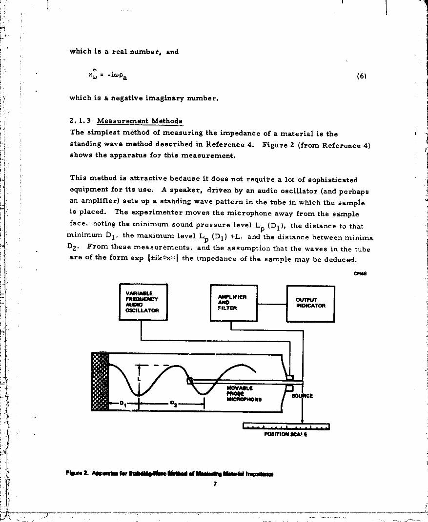
i 2. 1.3 Measurement Methods

i The simplest method of measuring the impedance of a material is the t!

_I

standing wave method described in Reference 4. Figure Z (from Reference 4)

_-- shows the apparatus for this measurement.

!.i: This method is attractive because it does not require a lot of sophisticatedi'

equipment for its use. A speaker_ driven by an audio oscillator (and perhaps

an amplifier) sets up a standing wave pattern in the tube in Which the sample

i is placed. The experimenter moves the microphone away from the sample

face, noting the minimum sound pressure level Lp (DI), the distance to that

minimum D I, the maximum level Lp (DI) +L, and the distance between minima

D 2. From these rr, easurements, and the assumption that the waves in the tube

are of the form exp _+ik*x'_ 1 the impedance of the sample may be deduced.

C_

ir [_ J

; VAFIL411LE AMPLIFlEAFREQUENCY ANO INDICATOR,NLJOIO FILTEROSCILLATOR

1

! 0 I

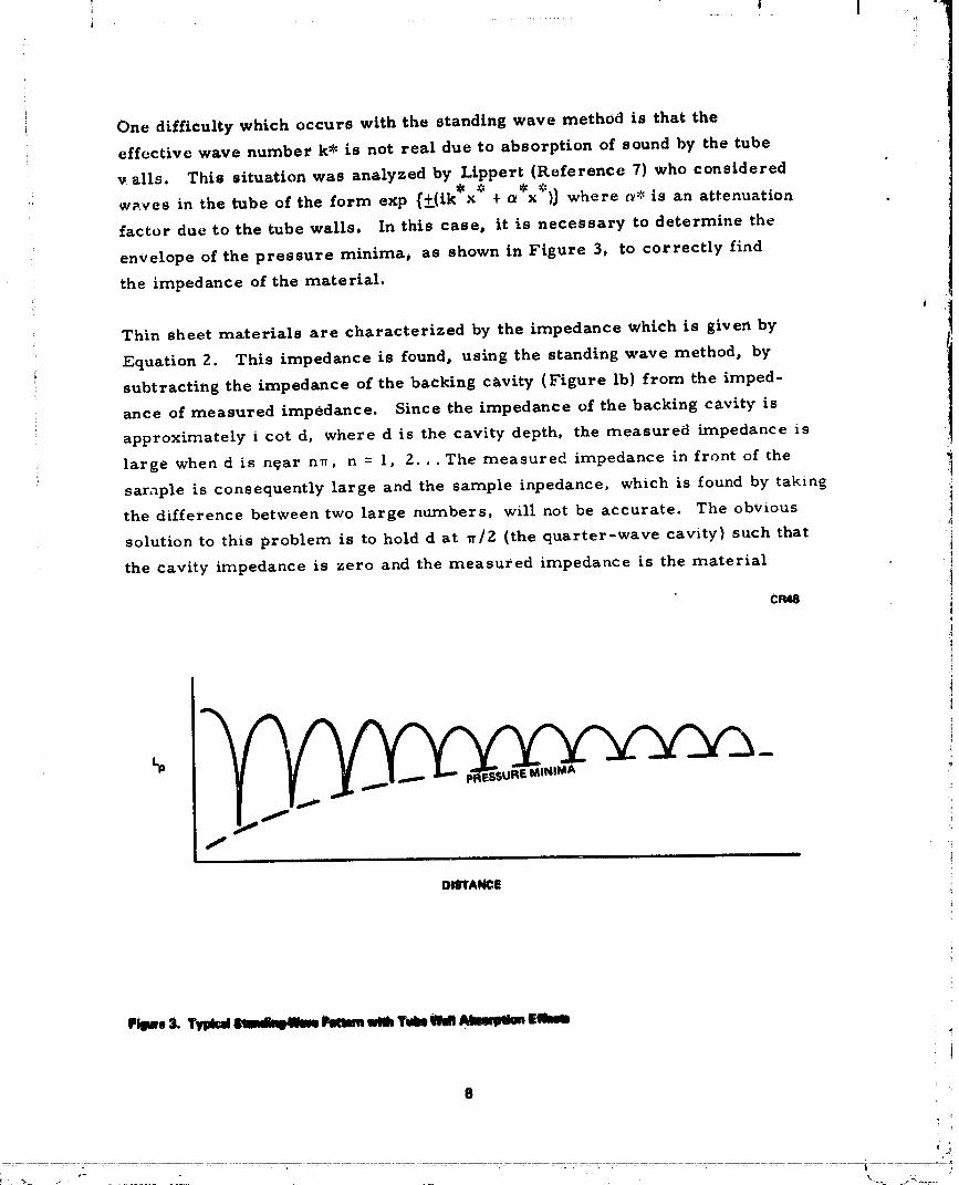
One difficulty which occurs with the standing wave method is that the

effectivc wave number k* is not real due to absorption of sound by the tube

v alls. This situation was analyzed by Lippert (Reference 7) who considered

{+(ik* * *x*)} where t_.' is an attenuation_v_,ves in the tube of the form exp x + _

factor duc to the tube walls, in this case, it is necessary to determine the

:: envelope of the pressure minima_ as shown in Figure 3, to correctly find

: the impedance of the material.

Thin sheet materials are characterized by the impedance which is given by!

Equation Z. This impedance is found, using the standing wave method, by

subtracting the impedance of the backing cavity (Figure lb) from the imped-

i ante of measured impedance. Since the impedance of the backing cavity is

i approximately i cot d, where d is the cavity depth, the measured impedance is

large when d is n_ar n_, n = I, 2... The measured impedance in front of the

saraple is consequently large and the sample inpedance, which is found by takin_

the difference between two large numbers, will not be accurate. The obvious

solution to this problem is to hold d at w/2 (the quarter-wave cavity) such that

the cavity impedance is zero and the measured impedance is the material

C_

L_ m

EssURE MINIMA :

'i

]I.j

.............. i i i , i i iii i i l

DllrfANCE

8

:i

1976024891-TSB06

impedance, While this is simple as arr, athematical conceptj it introduces

the practical difficulty ot adjusting the cavity depth to k/4 for each test

frequency.

A second method for measuring the impedance of a thin sheet is the

two-microphone method. As the name implies, an additional microphone is

added to th,, test apparatUs in Figure 2. This microphcne is fixed at the end _ _i

of the cavity and provides a measure of both the velocity through ':he thin

sample and the pressure immediately behind the sampie. The method also

requires an additional piece of equipment, a phase meter, to determine _I

the complex ratio of the pressure in front of the sample to the pl-es_Ure at I

the wall of the backing cavity. _

7_lelling (Reference 8) has given an extensive discussion of the design and

operation of a precision impedance tube using the standing wave method of

mea su r ement.

Melling also provides a brief discussion of the two-microphone method and

notes that its principal difficulties are errors in phase measurement, which

is an instrumentation problem rather than a fundamental defect of the

method, and errors due to placing one microphone at the face (in front of)

the sample. Melling was studying the impedance of perforated sheets and

the pressure field in the neighborhood of an array of orifices is very

nonuniform. This problem can be overcome by moving the microphone

back from the sample face a fraction of a wavelength. When this is done,

the formula for the impedance of the sheet is slightly more complex than if

the microphone were right at the sheet face, but the sheet impedance is

still given as a function of the complex pressure ratio between the micro-

phones. Like the standing wave method, the two microphone method works

best when the backing cavity is one-quarter wavelength in depth.

Bulk materials must be characterized by two complex constants, as shown

'/_ by Scott in Reference 5. There is a wide range of choices available for

13 which two constants are used, such as compressibility, sound speedj wave

number, characteristic impedance, or distributed impedance, however,

there _re only two independent constants. We have arbitrarily selected the

E

: J

, ... • . 1976024891-TSB07

i I i[

!=I

wave number (Equation 4) and the distributed impedance (_quation _) for use

i" in this report. Since there are two independent complex constants which

i characterize the material, at least four physical quantities related _o the

material sample must be measured. Scott (Reference 51 obtained the complex

i wave number (propagation constant) by moving a microphone through the

_::' hulk material while observing the signal of the microphone output and the

_i": signal from the driving oscillator on a dual beam oscilloscope. Figure 4I

shows a schematic of Scott's apparatus. The wave length was found by i

!i, moving the microphone until 360 ° phase shift occurred, and the attenuation

i' of the wave could be observed by the change of the microphone output as a

iJ_. function of distance_ These two constants are easily related to the complex

i_" wave number of the rnaterial. A modern version of Scottts experiment

would use a two microphone technique with a phase meter used to determine

the wavelength. The second complex constant used by Scott to characterize

the material was the characteristic m_pedance. This is the _mpedance at the

front of an infinitely deep sample of the material which can be measured by

the standing wave method.

c_

1976024891-TSB08

Z. 2 NONLINEAI_ IMPEDANCE OF THIN SHEETS

Up to this point it has been implied that the material impedance is independent

of the absolute amplitudes of the acoustic motion; by definition this should

be so since the propagation processes are described by acousticm or linear

equations. However, it has been pointed out that the propagation processes are

not considered within the material itself, as such; this is avoided by the use

of the material impedance concept. It turns out that the fluid motion near ]o

and within many lining m_terials of practical interestj at the sound pressure !Iamplitudes encountered in aero-engine ducts, is not a linear process and !

" i i

hence the impedance concept has to be used with care. _i _]: i!An effective liner impedance needs to be redefined; this is outlined in this •

: ! i

: section and the necessary types of modification of the linear material i,!

impedance parameters are described. It also appears that, although less

: well documented and understood, the effective liner _,_pedance is also a

function of the local grazing mean flow velocity. ,:!

When the fluid r,_otion within a lining material is accurately described by '_

linear equations it follows that a single acoustic wave incident on the liner

surface will be partly, absorbed and partly reflected, the frequency of the :J

reflected wave being the same as that of the incident wave. In addition the

impedance seen by the local sound field is independent of the incident wave ii

amplitude. In practice the impedance of most lining materials is dependent

on the incident wave amplitude and furthermore the frequencies of thei!

mution are not confined to the frequency of the incident wave. The existence

of nonlinear effects is corroborated by the zero frequency or steady flow

case where it is Well known that the mean pressure differential aci'oss a ' '

porous material at a sufficiently high Reynolds number is proportional to '

the square of the steady flow velocity. Based on this zero frequency case i

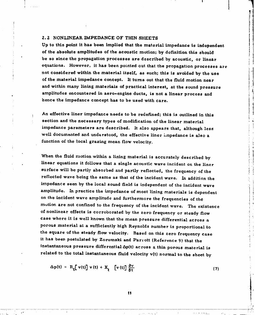
it has been postulated by Zorumski and Parrott (Reference 9) that the

instantaneous pressure differential Ap(t) across a thin porous material is

related to the total instantaneous fluid velocity v(t) normal to the sheet by

_p(t) : RtC v(t)J v (t) + Xt Ev (t)_ _)v (7)

iti I:

1976024891-TSB09

whore Rt Iv] is the measured steady flow resistance at the steady flowvelocity v, and subscript t emphasizes the dependence on time, t. Since

at high Reynolds numbers

RtEv3= blvl (sl

where b is a constant; it follows that (neglecting X t Iv(t)] for the present) , ,_

_p(t) = b v(t¿ Iv(t) I (9) JlSuppose now that only one frequence, wl, of fluid motion is present,

ivlt) - v I sinlt) 110)

(here t -- wlt*) then ,!

Ap(t) = bv_ sin(t) [sin(t) I (Ill i

or

f �bv_sin2(t),o __ t "<

/Ap(t) = (12) i

1 sinZ(t) !- by , w __ t -- ZTt i

Taking the Fourier transform of each side we get, following Zinn

(1_eference IO) and Melling (Reference 1 l)

8b-_ where Apl is the Fourier component of the fluctuating pressure differential

i at the fundamental frequency t_I. It follows that the impedance expressed as

?.J

" 1976024891-TSB10

a ratio of the pressure differential and the particle velocity at the funda-

mental frequency is

RI - v--_ = 3_ (14)

At sufficiently low Reynolds numbers R Iv] is independent of v

and then R I = a (16)

In general, both linear and non-lineax effects are present so that

Sbl' IR I _ a + 3_ (17)

This oversimplified example serves to illustrate tWo points: (I) that given a

particle velocity motion at particular frequency, fluctuating pressures at

other frequencies are generated when nonlinear effects are present (given

by the Fourier components at higher harmonics of the expression forAp(t))

and {Z) that an impedance can still be defined in the nonlinear case but it

is proportional to the particle velocity amplitude. In general, the particle

velocity motion will contain a wide range of frequencies and hence the

impedance at one frequency is influet,ced by motion at all other frequencies.

Thus, although the impedance parameter c_n stillbe defined in the same

way, itwill no longer be a function o_ the :-naterialproperties alone but is

a nonlinear function of the spectral distribution and 1-.velof the 1oca] sound

field (References 9, 12). One other point that is obscured in these intro-

ductory notes is that the particle velocity is not known, a priori, rather it

is an estimate of the sound pressure level. Thus, an iterative procedure is

required in general, although with certain assumptions this can be replaced

by the solution to a simple quadratic equation.

13

........1976024891'TSB11

_-. 2. I Perforated Sheets

A common approximation for the impedance of perforate_ is

- [a +bvo]- i If- hve] (iSl

where v is an estimate of the total effective particle velocity normal to

the material surface: b and h depend on the xn_terial geometry and mean

properties of the local fluid but h is also a _unction of v . For all tlJine

porous materials the parameter b can be determined from the bteady flow

resistance at large Velocity v. For perforate materials three similar

empirical expressions for b are available, one is given by Mariano

(Reference 13) as

The other expression, given by Rice (Keference 14), is bound up with the

definition of the total effective particle velocity which he gives as

Nf l/Z

v e = _._ i_ (zo)i---1

and v. is the effective particle velocity at frequency band i. With thoseI

definitions Rice (Reference 14) defines the parameter b as

b ; 1--- (zz)_Z

There is a similarity between the two expressions if we ignore the exponential

terms and note thatusuallv Z<<l; then they differ by a factor 1, 14/_ °' 1.

Also the exponential term in Rice's (Reference 14) expression has an argu-

114

i

\

1976024891-TSBi"2

I

ment which !8 of the same form as that in Mariano'_ (Refaronce 13) that is,

the ratio of a material length _cale (hole diameter or _hect thickness) and

parti¢l_ diap|acement magnitud_the

• expression al_o contains another exponential term, which i_ a function of

the hole aspect ratio J*/d_, which is absent from Rice's (Reference 14)

expression. The explanation for the former term is given by Rice

(Reference 14); he argues that when the fluid displacement is small compared

with the hole diameter the "jet will not fully form *t and hence the dissipation

will decrease. The choice of the hole depth as the significant length scale

• is seconded by Melling (Reference 1 1) who has shown that the nonlinear

resistance depends on the orifice discharge coefficient which_ in turn,

depends on the ratio of thickness to hole diameter• The origin of the terms

=

2: I l-or

_2 and o.2

in these expressions is, of course, in the well established, steady flow

expressions.

A link between these two expressions is found in that given by Armstrong

! (Reference 15):

IT

b -- l. OZ51 /exp -.507Z _*/d*-l.8 (Z3)

that is, it is very similar to Marianots expression except for the exponential

:i. term representing the dispiacemeL_ effect which is identical in form to that

. given by Rice (Reference 14). To summarize, there is clearly agreement

that the parameter b should be proportional to the inverse square of the open

area ratio but that is a11, apart from the consensus that a correction shouldP:

* be applied in the form _(fl_/v_ e) where t_ is a representative length or

_" effective thickness of the material (Reference 16). More work is needea

to establish a generally accepted, prerise form for this function and any

Ii other corrections which appear to be necessary.i_tl The correction for the nonlinear reactance h is based on experimental

observation such as by Ingard and Ising (Reference 18), Zorumski and

: :_, 15

.... "...... ....... 1976024891-TSB13

_:7' !

_ ! I Ix

I;+

i '

Parrott (Reference 9), and Mel!ing (Reference I 1), but no formulae appear

to ba generally available for this effec%

; The calculation of the effective particle velocity is, accardinp t- _ton_o(.I: a,tthors, bound up with the grazing flow eifocts.1+

I. 2. Z.Z Uniform Porous Materia._s

i' Parrott (Reference 91 have verified experimentally that the basic assunip:i,,:'

i of Equation 7 is correct, that is, the material properties are simply

:I described in the time domain by the measured functions Rt[v ] and X t [,'].

: These functions are the generalizations of the resistance and reactance use_

to characterize the material in the frequency domain. The spectral.

impedance Z w is not uniquely defined since it will depend on the incident

pressure spectrum in acomplicated way. For thin porous sheets of

material, it is believed adequate to assume X t [v(t)] is the constant

reactance measured in a low intensity test. The resistance R t Cv(t)_ can b_

measured in a flow resistance test since R t is a function of velocity only.

Assuming a line spectrum where Ap(t) and v(t) are given by

{ Ap(t)_ 124n-- _

an approximation to the spectral impedance is

= I /_' ~ i25)&Zn _r_ Rt[v(t) ] e int dt - inY; i

-W

where _ (t) is an estimated velocity. The velocity estimate may be the

result of solving the problem with the assumption that R t i s a constant which

is, in turn, estimated.

materials. Zwicker and Kosten (Reference 17) and Bies (l_eferer, ce 6)

express the flow resistance in terms of such things as porosity_ bulk

density, and structure factor, but these variables must be measured so this

equation is just pushing the measurement problem from one spot to another.

It seems preferable to regard I_t and X t as fundamental properties of and iacoustic material and fa :e the problem of measuring these functions i

directly.'!

/i2.2, 3 Measurement Methods

Measurement methods for nonlinear thin sheets are similar to the linear i

methods for thin sheets except that steps must be taken to account for the i

higher harmonics of the fundamental frequency which _re generated, either ]

by the material nonlinearity or by other nonlinearity in the experimental _'

device such as the acoustic driver in an impedance tube.

Ingard and ising (ReJ_erence 18) measured the impedance ot_ a single orifice :'

at the end of a tube by using a hot wire to measure the velocity in the orifice i

and a pressure pickup in the side of the tube near the orifices. A crude i

Fourier analysis of the signals gave the amplitude of the fundamental and ithe phase of the pressure relative to the velocity.

,

Melling (tLeference 8 ) has used both the two microphone method and the

standing wave method to measure nonlinear impedance of perforates. '

Narrow band filters were used to eli_ninate the higher harmonics such that

the standard measurcments could be made on the fundamental frequency.

This approach is not reliable, however, because, even though the filters

remove the higher harmonics from the measurement, these harmonics

still interact with the fundamental frequency in the material and affect the

measurement indirectly. If the acoustic driver is given a distorted signal,

or if the tube is operated near a resonant frequency such that shock waves

begin to develop, the measured impedance of the material will show these

effects even though the signals have been perfectly filtered. Thus, the :n_.easured impedance of the material is a function of the entire system

: properties and has no meaning as a material property at all. The solution

to this problem requires a redefinition of the impedance concept and an

improved experimental technique.

:-_ 17

" -'--" ] 978024891-T$C01

The new impedance concept required for nonlinear impedance was given by

Zorumski and Parrott in Reference 9, and is represented by Equation 7.

This impedance concept used a time domain expression for the material

property. The acoustic resistance and reactance, as given by Equation 7,

depend only on the velocity through the material. An immediate consequence

cf this assumption is that the acoustic resistance must not depend on the

fundamental frequency or the presence of higher harmonics in an impedance

tube test. This definition of impedance, if it is correct, is therefore a

material property which does not depend on the properties of the measure- t

ment apparatus as does the more conventional definition of nonlinear

impedance in the freqlaency domain. Zorumski and Parrott showed that

their definition does indeed represent a sample of material over a wide/

range of test frequencies and intensity levels, from zero frequency, the _7dc flow resistance, to a 4,000-Hz fundamental frequency test. The I

measurement method used in this test was the two-microphene method with ..... _!

the backing cavity adjusted to one-fourth of the fundamental test frequency

wavelength. The microphone signals were Fourier analyzed and the t

instantaneous pressure differential, velocity through the sample, and iacceleration through the sample were found to determine the resistance and

reactance functions in Equation 7.

The preceding discussion shows that the spectral impedance of a nonlinear iij

material depends on the entire frequency spectrum. Wir* (Reference 19) irecognized this intuitively and defined impedance as follows: "The impedance

at the surface of a nonlinear acoustical material is the ratio of the pressure to 'i

the particle velocity, at a particular frequency, and in the presence of a speci- o_

fled sound spectrum and a specified turbulence spectrum. " Wirt regarded

the effect of flow as causing turbulent pressure fluctuations which would ,_

induce a normal velocity through the material. Although he had no convenient

way of simulating the flow effect, he did devise a method of measuring imped-I

ance, by the standing wave method, in the presence of an intense broadband

spectrum. Wirt_s impedance tube used three drivers to generate a broadband

_' spectrum of specified shape and intensity,while a fourth driver added a pure

i_ tone _vhichwas used for the impedance measurernent. One-third octave band

and I.8-Hz bandwidth tracking filters,tuned to the oscillator frequency were

1976024891-TSC02

I

Q

used to recover the tone standing Wave pattern. Note that if v (t) in Equation

l 25 in an intense broadband spectrum, Equation Z5 represents Wirt's defi-

nition of the impedance.

Z. Z. 4 Linearization of Impedance

in this and the previous Section the particle velocity normal to the liner

surface has appeared in formulae for nonlinear modifications to the liner _

impedance and the same quantity is also used by Rice (Reference 14) to _I_,

relate the flow-induced pressure fluctuations to a flow-induced modit_ication ,j

to the linear impedance, ii

This quantity is not known a priori in practical applications nor is it easily

measured; the same is true, in fact_ foi" the sound pressure level although ,,

it is relatively easy to measure and the existence of nonlinear effects makes

it essential, at least, to estimate the sound pressure level at, or near, the Ji

liner surface. The relationship between some sound pressure level and the _

particle velocity iS often glossed over in the literature; sometimes the i!I!

p'lane wave relation is used (without justification) so that ! :

v = pJ%c (26) it_ a

where p_ is the pressure amplitude, but of course the correct relation is i

* t0*/Pac Zv = P a to (Z7)

"i

(by definition). Two problems immediately arise: the pressure p_ is the

complex amplitude actually at the lined surface and is, itself, a function i

of v*. It is not the pressure amplitude in a hard-walled duct and in principle ito

it is not known until• it can actually be measured with the liner installed. A

further complication is that the particle velocity, it is argued, at one

particular frequency should be replaced by a total effective particle velocity

when using the nonlinear impedance modification formulae, since the

nonlinear bias is a response to the particle velocity at all frequencies. Thus,

Kice (Reference 14) and others have defined the total effective particle

velocity to be

19

i..,_

_7'. _ _"

1976024891-TSC03

• i 12]''2= v (Zo)Ve i=l

where

::_ Piv. = (Z9)

l IPaCaZl I

(the i subscript denotes a frequency or frequency band and the surr:rnation is

over all the frequency bands which may contribute a significant vahe for

p_i ). In this case P_i the pressure amplitude in frequency band iiI assumed

known. Notes however, that Zi = Z_ is calculated using expressions of

the form

Z_: [a +b iVel]- i[g- h lVel] +icot(k*d*) (30)

i Then v* i and hence v* is calculated using the previous two equations which! e

i complete." the first loop; with the new value of v tbe impedance Zc_ can bee

! recalculated and the iteration repeated until two successive values of Z_

I are nearly the _,ame.

In principle, of course, the pressures P_i are not known and incorrect trends

may be obtained from assuming that P_i is R constant in these iterations. It

is preferable, following Ingard, (Reference 18) towork in terms of an

incident sound pressure amplitude, P_i' and then the particle velocity v*.l

is given by

... 2P0 i

Twice the incident pressure amplitude, Zp_i, can be loosely identified with

the pressure amplitude in frequency band i in a given duct system when the

duct walls are unlined.

_0

1976024891-TSC04

2.3 THE EFFECT OF GRAZING FLOW

2.3. 1 Empirical Models

There is at least one physical effect of sheared mean flow on sound propa-

gation and attenuation in lined flow ducts which is well established in that

- it has bee_ extensively studied, at least analytically. Physically it is the _ _refraction and convection of sound by the mean flow. This effect, when

included in the propagation equations, yields calculated values for, say, the ii imodal attenuation rates which do no.__tappear to agi-ee with experiment (Kurze _ i

and Allen_ ReferenCe 20), unless a modification is assumed for the liner i i

impedance, in addition, from certain experiments_ measured liner

impedances in the presence of grazing flow confirm that a modification

appears to take place although all experiments to date have been questioned

.......... t_certain respects. While measured attenuation rates do strongly indicate

some sort of modification this .may be an incorrect interpretation insofar

: as there may be other physical effects which ai-e not accurately represented

in the p1"opagation equations. However, for the present, this semfempirical

"• effect is accepted and expressed as a modification in the form of an

additional term, to the zero-flow impedance. Incidentally, there is no

a priori reason why an additive term for the impedance is appropriate. It

could be equally well that an additional term for the liner admittance is

./, appropriate as, for example, in the case where viscous effects on duct

_,. propagation are represented in the form of an additional admittance

i: (Referetlce 2 1).I

Kurze and Allen (Reference Z0) state that "the reactive component of a lining

with perforated plate has to be reduced and the resistance had to be chosen

hi_her than the liner acoustic resistance of the particular material" to

obtain good agreement between experimental and theoretical attenuation

rates. They "assume that the resistance of a nonlinear material increases

with sound-pressure difference across the lining" but that "the observed

proportionality factor between the nonlinear influences of flow and sound is

hi_her than expected from turbulent pressure fluctuation at a smooth hard

wall .... The (measured level) is at least 10-15 db lower (however) than

the equivalent level . . . (but) recent data show that the roughness of

a wall can substantially increase the wall pres3ure fluctuations. " They

21

" 1976024891-TSC05

!

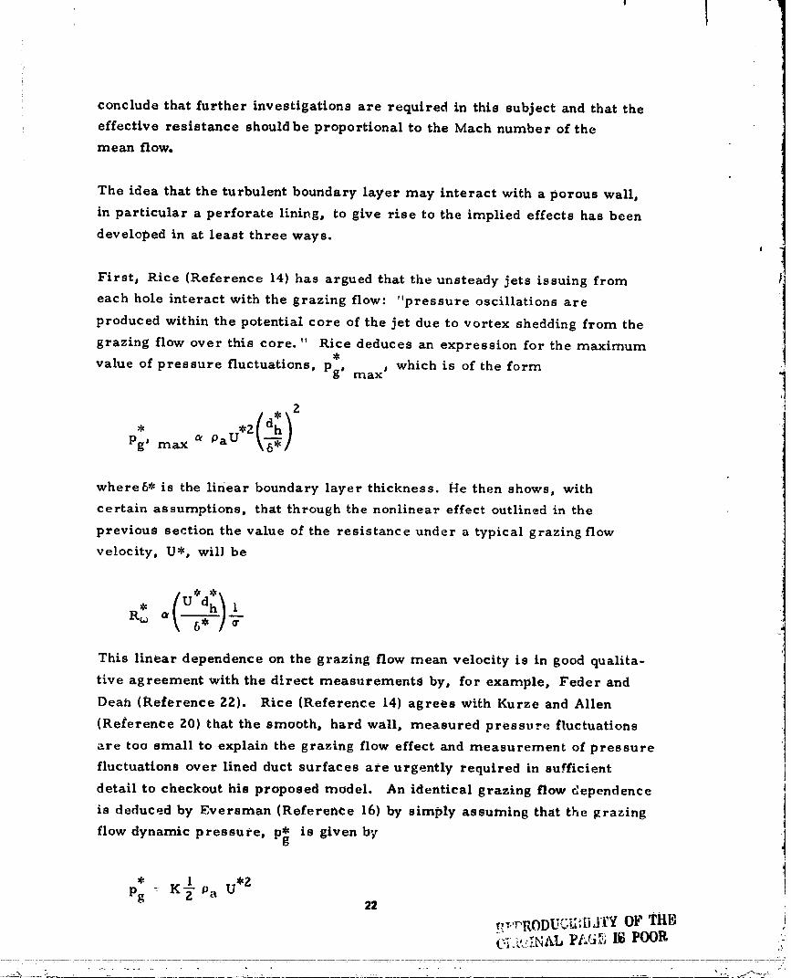
conclude that further investigations are required in this subject and that the

effective resistance should be proportional to the Mach number of the

mean flow.

The idea that the turbulent boundary layer may interact with a porous wallj

in particular a perforate lining, to give rise to the implied effects has been

developed in at least three ways.8

Firstj Rice (Reference 14) has argued that the unsteady jets issuing from

each hole interact with the grazing flow: "pressure oscillations are

produced within the potential core of the jet due to vortex shedding from the

grazing flow over this core. " Rice deduces an expression for the maximum

value of pressure fluctuations, pg, max' which is of the form

• oPg_ max Oa U*2 \'6"*/

where6* is the linear boundary layer thickness. He then shows, with

certain assumptions, that through the nonlinear effect outlined in the

previous section the value of the resistance under a typical grazing flow

velocity, U*, will be

'i

This linear dependence on the grazing flow mean velocity is in good qualita- !

tire agreement with the direct measurements by, for example, Feder and

Dean (Reference Z2). Rice (Reference 14) agrees with Kurze and Allen ii

(Reference 20) that the smooth, hard wall, measured pressure fluctuations

_re too small to explain the grazing flow effect and measuremen_ of pressure

fluctuations over lined duct surfaces ate urgently required in sufficient

detail to checkout his proposed model. An identical grazing flow dependence

is deduced by Eversman (Reference 16) by simply assuming that the grazing

flow dynamic pressure, p_ is given by j

• 1 tPg _ K T Pa U *z ]

_2

• ,-',," ' oFTHB ip .'rRODU_,Li,bA[ ¥......, "_"Ikb

1976024891-TSC06

I

I

where K is a function of the grazing flow boundary layer, face sheet surface

geometry, and roughnessj and is determined empirically.

The second approach is that developed by Ronneberger (Reference 2_)

originally for the case where the hole diameter is larger than the boundary

layer thickness. Based on the concept that the whole boundary layer

fluctuates in and out of the orifice and on information concerning the

instability of this motion, Ronneberger deduces that the real part of the

orifice impedance is proportional to the grazing flow velocity, which is

borne out very clearly by his measurements. The dependence on boundary

layer thickness is not deduced in detail from his theoretical model, but he

argues that it is of the same form as that deduced by Rice (Reference 14),

if 6*/d_ << 1 and _5*fU* << I. It should be emphasized that Konneberger's

work is mainly concerned with the case 6*/d_<< 1 and that his postulatedn_echanism differs from that of Rice (Reference 14) in that the latter author

appeals to the nonlinear response of the perforate whereas Ronnebergerviews the effect as a flow induced change in the radiation impedance of a

single orifice.

Another mechanism has been proposed by Hirata and Itow (Reference Z4)

based on the argument that the kinetic energy of the motion in the vicinity

of the orifice is "carried away" by the airstream and thus since energy

"dissipation depends on the diffusion of energy from the resonator into the

surrounding meal±urn" the dissipation (by the orifice) depends on the

(grazing) airflow. They develop simple equations to describe these energy

related concepts and deduce the same dependence on airflow velocity as the

previous authors r._entioned above. They use their formula for the flow-

induced resistance in transmission loss calculations which they compare

with measurements for mean-flow velocities up to 50 m/s and find

reasonable qualitative agreement.

Another feature of the flow induced change in acoustic material properties

is given by Budoff and Zorumski in Reference Zf. When there is a tangen-

tial flow on a side of a thin sheet, it cannot be assumed that the resistance,

R, for blowing into the stream is the same as for sucking from the stream.

The flow resistance of perforated sheets was therefore measured with both

1976024891-TSC07

' I

blowing and sucking and the results Were compared. It was found that therc

was an added resistance which is proportional to tangential velocity, as in

the previous discus_Bion) but that the factor of proportionality was not

the same for blowing as it was for sucking. These results, illustrated in

Figure 5, were not explained and are in need of independent confirmation.

cN

iR

i

M>O

M _0 / •,f

Id=O M-O

-

Figwe IL _ of Flow Resistmweof PerfonmdShooton Tenientid Idlh No. M (-U*lc o) andNorn_NO.. v. NOlI_VO v IndiautosBoundaryLawyermowingi PosI_Ivov IndiatN Suction

_xperiments with a single orifice in the presence of grazing flow

_Reference ZZ), however, still show a close correlation between acoustic

resistance and flow resistance. This correlation can be explained from the

study by Posey and Compton (Reference Z6) which shows an equivalent

resistance can be defined in terms of the resistances for blowing and

sucking. This equivalent resistance is a weak function of the difference in

the actual resistances and is roughly ZR+R./(R+�R I, where R 4 is the

resistance for sucking and R is the resistance for blowing.

Some unpublished measurements were made by Feder (Pratt & Whitney

Aircraft, East Hartford, CN) of the flow resistancc of perforated sheets in

the presence of tangential flow. Feder's data were subsequently correlated

24

_"?_ODU?:!.;__j'i'Y OF Till';

I;i ,:",'I_),, _`_..'-'" _; pl')_)_

........... %

1976024891-TSC08

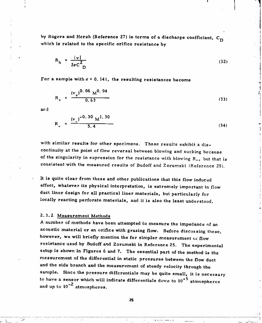
by Rogers and Hersh (Reference 27) in terms of a discharge coefficient, C Dwhich is related to the specific orifice resistance by

• IvlRh - 2 (32)

2o'CD

For a sample wither= 0. 141, the resulting resistances become

I1

(v+)O. 06 M O. 94 ;IR+ = 0.63 (33) i

,t

at, d !

(v_)-O. 30 MI. 30"

R_ = 5.4 (34) i

with similar results for other specimens. These results exhibit a dis- i

continuity at the point of flow reversal between blowing and sucking because 1

of the singularity in expression for the resistance with blowing R_, but that is !iconsistent with the measured results of Budoffand Zorumski (Reference 25). t

i

,. It is quite clear from these and other publications that this flow induced

effect, whatever its physical interpretation, is extremely important in flowI

duct liner design for all practical liner materials, but particularly for 1

locally reacting perforate materials, and it is also the least understood, i.4

2, 3,2 Measurement Methods

A number of methods have been attempted to measure the impedance of an

acoustic material or an orifice with grazing flow. Before discussing these,

however, we will briefly mention the far simpler measurement o_ flow

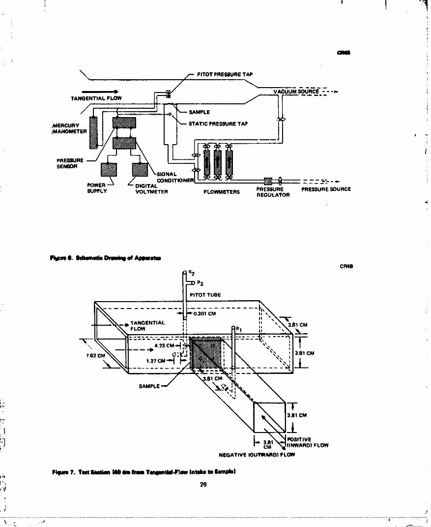
resistance used by Budoff and Zorumski in Reference 25. The experimental

setup is shown in Figures 6 and 7. The essential part of the method is the

measurement of the differential in static pressures between the flow duct

and the side branch and the measurement of steady velocity through the

sample. Since the pressure differentials may be quite small, it is necessary

to have a sensor which will indicate differentials dcwn to 10 -5 atmospheres

and up to 10 -2 atmospheres.

2§

1976024891-TSC09

Crab

_,_ _ PITOT PRESSURETAP

r--"(ii/ VA( _UUMSOURCE " " "="

TANGENTIAL FLOW I_JII _ I

Sl

_WER_ ZOIGITA_N°IT_N'RI_ _ _ ....PRESSURE PRESSURESOURCE

SUPPLY VOLTMETER FLOWMETERS REGULATOR

1

Filun 1. Tut _ Ill It ItII TIlmtid,F_i Intake to bmpto)

!=_ 26

1976024891-TSC10

: I I _qI

-_:t A similar large range of flow rate is required. This was accomplished by

-i"!_ using three rotameter flow meters with a suitable pipe and valve arrangementt_

I: as showll on Figure 6. This system also utilizes the same flow meter forboth blowing and sucking flow rates, so that any asymmetry observed in

' the resistance cannot be due to switching flow meters.

Fede1' and Dean (Re_erence 2Z) measured the impedance of thin sheets in

the presence of grazing flow using the standing wave method. The sample

: was mounted in the side of a small flow duct, as in Figure 6, and the side

:" branch was used as an impedance tube. The principal difficulties of this i

method were accurate measurement of the standing wave pattern and

uncertainty about the radiation impedance of the tube, looking into the

flow duct.

Ronneberger (Reference 23) used an apparatus similar to Ingard and Ising's

(Reference 18) to measure the radiation impedance of an orifice looking into

a shear flow. Some cZ his results have been discussed previously in this

report. We note here, however, that Ronneberger found that the acoustic

resistance and flow resistance of the orifice were nearly identical and that

the reactance decreased with increasing tangential flow.

Armstrong, Beckmeyer, and Olsen (Reference 2B) measured the impedance

of a wave in a flow duct with one treated wall by measuring the axial wave-

length and decay rate of a duct mode with a two-microphone technique. The

apparatus is shown in Figure 8. In this method, the shear flow profile is

measured and the shear flow wave equation is solved to relate the duct liner

impedance to the measured axial wave number. The advantage of this method

is that it tests a complete duct liner under conditions simulating its intended

application. Its disadvantages are that it requires large material samples

and an elaborate data reduction _cheme. (Also, it does not appear to be

easily extended to the measurement of nonlinear impedance. )

Dean (Reference 29) used a one-microphone method (not previously discussed

here) and the two-microphone method to measure the impedance of duct

liners in the presence of flow. Dean's results indicated that the two-

microphone technique was preferable. This method has the advantage of

bein_ applied to a finished duct liner, like Armstrong's method, and ha_J the

j_ added advantage of being able to measure nonlinear impedance.

_ll 27 ,

1976024891-TSC11

2e

1976024891-TSC12

;i

_..t I_I,:t:__MMI,:NI)I,II) MI,:'rtlOD_ FOR MATERIALS

Ihtlk II_._lt'l'i.tl_ ar_ nt)t _flen used in aixcraft engine duct applications,

howt,vt',', !ll_,ir title i_ always a possibility 8o that they should be included

in .uw pr_.dicthm scheJ_e. Little is known abouL nonlinear behavior of bulk

materk_is. The work mentioned here has been concerned with linear

properties. ThLs linear representation may be acceptable in the aircraft

engine application because a bulk material in a duct liner weald probably be I i

protected by a facing sheet which would cut down on the amplitude of theI

waves in the material. For prediction purposes, therefore, it is

recommended that:

Bulk materials are assumed to be linear and described through the equations

_p_ * zwv _ -- 0 (35)

and

2p_ 2V + k P_0 = 0 (36)

where zto and kw are experimentally measured complex material parameters

which are functions of frequency.

Sheet materials which are essentially rigid, both perforated sheets and

uniform porous materials, are typically used in aircraft engine as facing !4

sheets which are exposed to high intensity sound and to grazing flow. It

has been demonstrated many times that there is a _lose correspondencebetween measured acoustic resistance (in ,_he frequency domain) and flow

resistance. Also, time domain measurement,_ have shown this equivalence

between flow resistance and instantaneous resistance for intense waves

with fundamental frequencies up to 4,000 Hz. Therefore there is no

question that the quasi-static assumption is valid over the entire range for

_- which measurements can be accurately made. Less is known about the

_' reactive part of the material impedance. This term is always small com-

_t pared to the resistive part at high amplitudes so that it is extremely difficult

....I_ to measure; however, since it is not a dominant effect there is little motiva-J

tion to measure it and, as an approximation, it may be assumed to be inde-

dendent of level, that is, the reactive part of the material impedance is linear.

29

[

1976024391-TSC13

i i;

It is known that graz_tng flow affects the resistive part of the impedance of a

;_ thin sheet. The effects seems to be directly proportional to grazing flow

; velocity tin the free stream) and inversely proportional to boundary layer

thickness. It also seems that the proportionality constants ,_fthe flow

resistance are slightly different for boundary layer blowing than they arei

for boundary layer suction. This difference implies that there is a peculiar

i_' sort of nonlinearity induced by the grazing flow, even at low sound pressure ,levels.

i. I

i?!i, The following expression is recommended to represent the acoustic

i("

i!i properties of all thin sheet materials:

Ap = Ztv* (37)

whe re

. {[ (01:a)l 0 ,.aZ t = 0aC a R v, M, + _ Pa Ca 0t* (38)

The nonlinear resistance R is to be measured in a steady flow resistancc

test. The normal velocity v_'-will have the range 10-4 .<.[v:'.:/Cal< I0"z in

< 0, M>0) and suction (v_'/c >0, M > 0) measurements.both the blowing (v_/c a aThe free stream Mach number shall have the range 0<M<0. 5 and the

boundary layer displacement thickness shall be chosen to correspond to the

intended applications of the data. The measured data are to be correlated

in terms of a discharge coefficient, in terms of which R is given as

R - IvL_ (39)202 2

C D

(" and the discharge c oeffici__nt shall be asymptotic to _ if Iv [<< M

l and to a constant when I v I is of the same order as M. In addition, R is

taken to approach a constant when both M and Iv I are small. The reactive

part of the impedance, Xe, may be measured at a low intensity- < 120 d B) by either the standing wave or the two microphone

(100 db _ Lp _

-_i! 30

1976024891-TSC14

method, with the material placed in front of a quarter-wave backing cavity.

The impedance is to be linearized by computing an effective velocity !

i

Ve _ vi I 2 140)i= 1

11 = 2 R[+ Ve] R [-Ve] (41)e el + R[-v ]e

so that the material impedance is

Z_Z_ : R e - i_ 0e_ (42a)

or

A Z : R e -iX e (42b) _ ]

If X e is measured at only one frequency, the expression in Equation 42a can

be used to calculate AZ_ at any other frequency by assuming _, Oe and _I

_*Ica)" _are frequency independent (note _ = However_ it is preferable i'1

to take measurements of X at all frequencies of interest and then to usee

Equation 42b. i1

31 "

1976024891-TSD01

Section 3

DUCT LINERS

3.1 FLAT POINT REACTING LINERS

Under certain conditions the impedance normal to and at. the lined surface

is a function Of only the liner parameters, except fo_ certain local mean

flow properties such as the mean density and the coe£ficlent of viscosity.

In particular, when it is independent of the p_operties o£ the local sound

field (apart from its frequency) the lined surface _s said to be point reacting.

PhySically, the simplest feature of point reaction is that the direction o£ t

acoustic motion within the liner is independent of the direction of an incident

plane wave.

The impedance normal to and at the sur£ace of a flat, point reacting single-

layer configuration (backed by an impervious, rigid wall) is o£ the form.

Zoj = A Z_ + i ka/k_;'_ cot(k3._d*l (43)i

iThe second term is the impedance of the air-cavity under these conditions

where d__ is the cavity depth and k _,_is the wave number of the motion in that

cavity. In most applications it has been assumed that this motion is in the

form of a plane wave so that k::"= k a - c_/c a. lVielling (Reference 11) hasnoted that. due to viscous and other dissipative effects on propagation within

the honeycomb cavity it is preferable to assign a small imaginary part to

this wave number, which could be obtained from impedance tube or in situ

measurements. If only viscous effects are taken into account then (Ref- l

erence 11) k ::_is given by I

1

k'_ : -- + :,_ _'_'_') (44) ',ca re a

where r_ is the effective radius of the honeycomb cell and v is the kinematic

viscosity of the cavity fluid. The general form of the alr-cavity impedance

expression is for the case when the cavity walls are normal to the porous

sheet surface. Appropriate modifications are needed if th_ cavity has a

variable cross-sectional area and/or the walls are not normal to the porous

sheet. Developments in this direction are being pursued by Wirt (Reference

30) for complicated but point reacting liner configurations which have c_esir-

able features such as good low frequency absorption relative to standard I

configurations of the same depth, and wide-band absorption characteristics

_ previously thought unattainable with their porous material cavity combination.

The locally reacting liner may be of the multilaye1" type, that is, made up

il of a number of porous sheets separated by honeycomb layers o£ various _

_Ii dew.hs. For simplicity we consider the fiat single layer type although, in

i principle, the information summarized here can be applied to convex and ii concave, multilayer_ locally reacting configurations; general expressions

for _he impedance of those configurations are given by Zorumski (Ref- !I

erence 31) in terms of the linear hnpedance of each material layer and the

distances between or depths o£ each layer. Following the analysis of Zwicker

_nd Kosten (Reference 17), it can be sLown that the impedances of successive

!avers of a duct liner are related by the recu:'rence formula !'i

o "I &Z_ "cos kwd oJ

kw (45) i

"k_sin k d 'I• z w cos kwd v w :i

0 I _

where , 1

• - -i, -- I

if _he medium within the honeycomb cavities is at ambient conditions.

] 97602489]-TSD03

3.2 FLAT EXTENDED REACTION LINERS

In general, the liner impedance concept is most useful when the liner is of

the point reacting type. At the other extreme when the normal impedance

at the lined surface is, say, a function of the angle of incidence but still

independent of position, the impedance concept can still be used to some

advantage, as outlined below. However, in order to incorporate the more

realistic case when the impedance is a function o_ position, the impedance

concept, per se, can be discarded in most extended reaction cases in favor

ot a different approach. That is, sound propagation through the liner itself

is included in the description of the wave pi'opagation throughout the duct.

The boundary condition for the wave prop, _tion process is still in the form

o£ an impedance or admittance parameter, but the surface at which it is

applied is elsewhere such that point reaction can still he assumed.

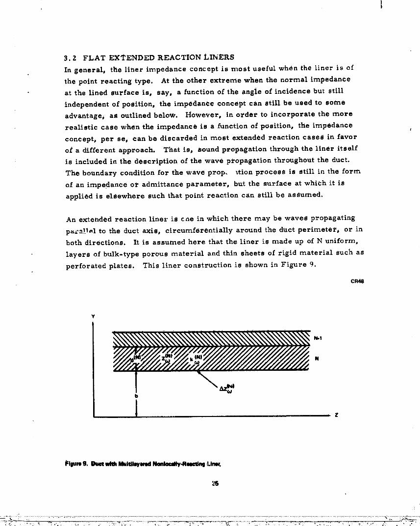
An extended reaction liner is cne in which there may be waves propagating

p_i-_X!_.l to the duct axis, circumferentially around the duct perimetei'j or in

both directions. It is assumed here that the liner is made up of N uniform,

layers of bulk-type porous material and thin sheets of rigid material such as

perforated plates. This liner construction is shown in Figure 9.

CR48

Y

N.I

N

b

Figureg. DuetwithIdultUsyemdNmdacdly.HeeetingLiner,

,_ _ m, .......... .. , .... , v ..... _....... :_ _.,_._/_,_

1976024891-TSD04

When duct liners are sufficiently thin for curvature effects to be neglected,

their analysi_ may be carried out in ret_tangular coordinates. In this case,

the wave numbers are related by

(n) Z . (n) 2(krm) - (_) - (kzm)2 - (m/b) 2 (46)

!

Following the analysis by Zwicker and Kosten (Reference 17), it can be illshown that the pressures and velocities o£ successive layers of the duct

liner are related by the recurrence /ormula (Equation 45) if k (n) iS sub-

(n rmStituted for k ). H the liner is partitioned so that wave_ may not travel

axially, kzr n iS set to zero, and i£ they may not travel circumferentialiy,

m is set to zero. Thus, Equation 45 provides a means of calculating the

surface impedance of uniformj multi-layered extended reaction liners.

Through Equation 46 the surface impedance o£ such a duct liner may be a

function o£ the circumferential and/or axial wave numbers. This generally

presents no difficulty as far as the circumferential wave number is concerned,

since the acoustic equations in axisymmetric ducts may be solved separately

for each circumferential wave. However, the impedance Equation 45 must

be evaluated simultaneously with the appropriate duct propagation equations

and kzm will be variable during the solution process.

3.3 RECOMMENDED METHODS FOR LINERS

An iteration process must be u_ed to compute liner properties since the

impedance depends on the acoustic spectrum through Equation 40. Here we

assume that a one-third octave band spectrum of Pw is known at the linear

surface. The first step is to compute the resistances of the mater_.al layers

i_ from some estimate of the corresponding velocities. This information is

:'_ then used to re-estimate the velocities. The process may be started by

i_ assuming all velocities are small so that the material impedances or resist.

!l antes are independentofvelocity. Thus, for a linerwith N layers, we start

with the velocity vector for each frequency or frequency band i

1976024891-TSD05

f vl N) 10 -4

[ v(I) lo .4

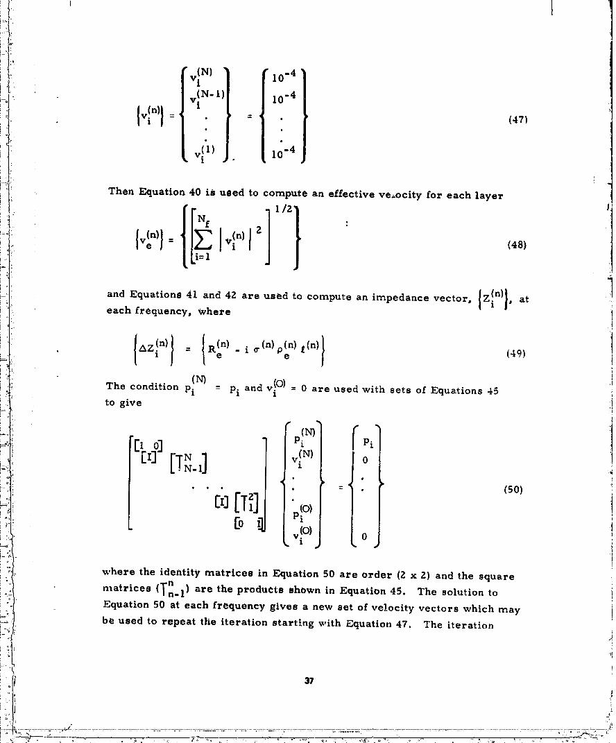
_ Then Equation 40 iS uBed to compute an effective ve.ocity for each layer

-- I (48)

and Equations 41 and 4Z are used to compute an impedance vector, {zln) }, at .'I

each frequency, where

_Z! n) - R (n) - i cr (n) 0 (n) t (n) l (49)1 e e I

(N) v (O)= 0 are used with sets of Equations 45The condition Pi = Pi and i

to give "

• (I'_"'- Pi

o

.... [I.] [].2][oI "plO),,!o),j = :loJi (_o)

where the identity matrices in Equation 50 are order (Z x Z) and the square

matrices (T_.I)._are the products shown in Equation 45. The solution to

Equation 50 at each frequency gives a new set o£ velocity vectors which may

be used to repeat the iteration starting with Equation 47. The iteration

37

t! , o ,, p ,, ,_: ,, : , H 1976024891-TSD06

stops when the effective velocity vector ceases to change by a significant

amount with successive iterations (or, alternatively, the resistance vector

as described in Section 4).

3.4 EXAMPLE LINER

Reference 3Z describes the inlet liner for a typical ground test nacelle ....

The liner is a perforated plate, 0.5-ram thick, with 1. Z7-mm diameter

holes spaced to achieve an open area cr = 0.068. The backing is honeycomb

with a 12.2-ram depth. The needed flow resistance and effectivedensity l!

function for the plate is not known, however they may be estimated. For

flow into the liner the orifice discharge coefficientis assumed to be

0. 8 _(Reference 27) and for outflow it is taken as _/ivl/M. The corre-

sponding orifice resistances are M/1. 28 and M/2.0 and the acoustic resist- ,,,

ances (based on average velocity through the plate) are R+ = M/0. 087 for

inflow and R _- M/0. 136 for outflow. The effective density is taker_ to be the

air density so that Pe = 1. The inlet machnumber is 0.58 so that the effec-

tive resistance is R r = 5. Z0. The reactance in Equation 42 is negligible so

that Equation 43 gives an impedance of

Z = 5. 20 + i cot (Z. 253X10"4f),t_

which is 5. Z0 + [ 4. 36 at f = 1 kHz.

' _ ",Ix."

1976024891-TSD07

Section 4

RECOMMENDED PREDICTION METHODS

4. 1 SINGLE-LAYER LINER CONFIGURATIONS

The calculation method falls into two parts. The first is concerned with the

. cavity impedance, which is assumed to be independent of sound pressure

level and grazing flow effects. The second involves an iteration for the sheet

material acoustic resistance which is dependent on those effects and which

also utilizes the calculated cavity impedance. Input data for both calculations

is summarized first, under the data base heading.

It should be noted that symbols like Zi, PiG and v i have been replaced by

Z(fj), po(fj) and v(fj);that is, vi, for example, at frequency band i is now

particle velocity v(fj) at the frequency band j for which the center frequency

is f.. This not only serves to provide an explicit reference to f. (and pre-J )

vents confusion between i = \-I and the frequency number), but it dis-

tinguishes the parameters used here from their counterparts elsewhere in

the report which are often single frequency or spectral (Fourier} quantities.

Also is should be noted that, in general, the cotangent function in what follows

and the parameters k-':-'(fj),z-'::(_),Zc(fj), kzm; k::.'rm,_Z(_) and v(f.) arecon_piex quantities.

!Data Base

1. Center-band frequencies fi' j = 1, 2 . Nf, Hzt$

2. Speed of sound in duct medium, Ca, m/sec

_ 3. Characteristic impedance of duct medium, PaCa , ._IKS RAYLS

4. Sound pressure level spectrum in hard-walled duct, SPL H (fj),• db re: Pref = 2 x 10 "5 N/m z

l 5. incident (normilized) sound pressure spectrum:po(fj) = I0 j XPref/PaCa

2 from (2), (3)with SPLIt(fj) from (4), PaCa

..........................- ....................................................................................................................................................................................................................................

] 97602489]-TSD08

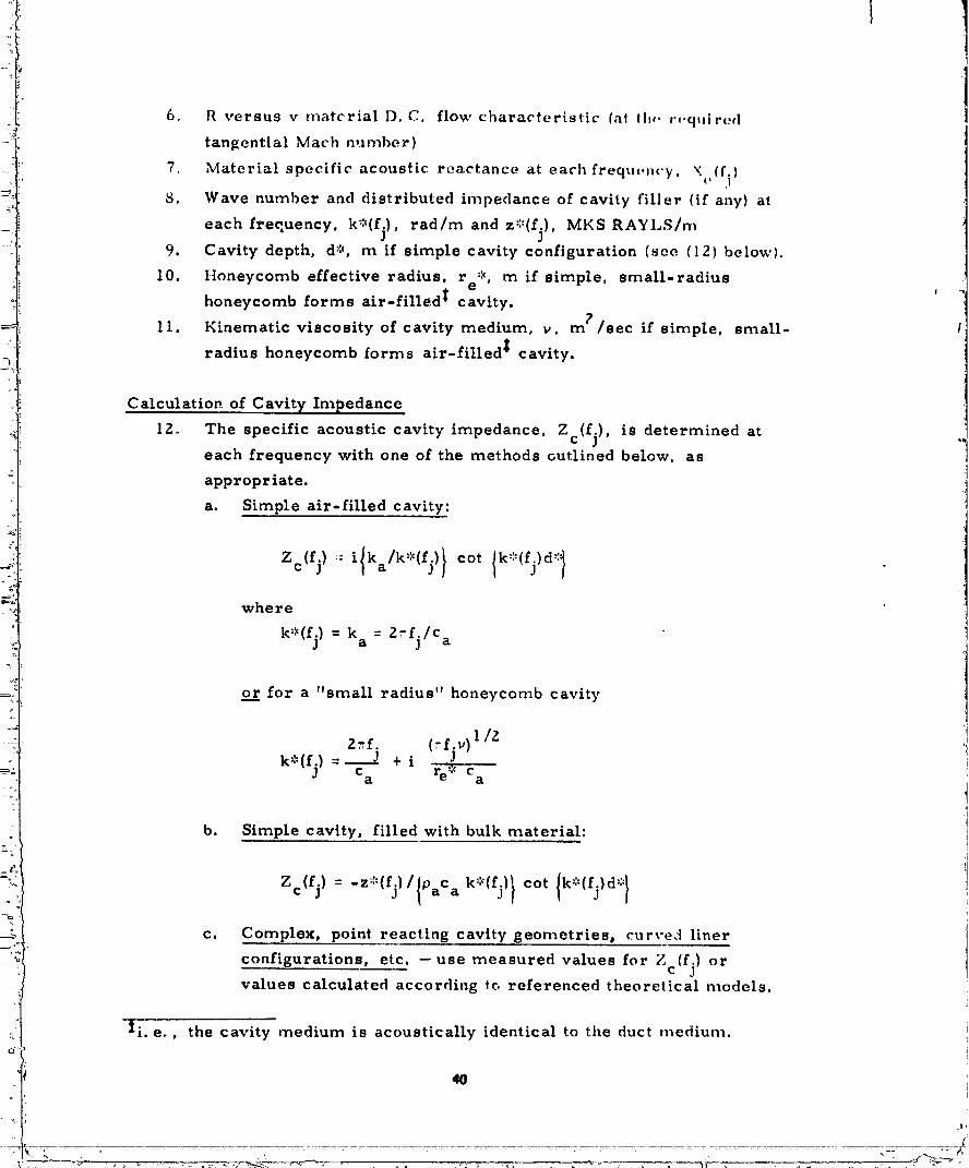
i! •.16. R versus v material D.C. flow characteristic (at tlJ,. ra.quired4

• tangential Mach number)

7. Material specific acoustic reactance at eachfrequ,,,i,.y. X {fj)

8. Wave number and distributed impedance of cavity filler (if any) at

each frec, uency, k::,(fj), rad/m and z::'{fj), MKS RAYLS/m9. Cavity depth, d':L m if simple cavity configuration (see 112) below).

.t

10. Honeycomb effective radius, re-.,, m if simple, small-radius |

honeycomb forms air-filled $ cavity.?

11. Kinematic viscosity of cavity medium, v, m /sec if simple, small-

radius honeycomb forms air-filled $ cavity.

Calculation of Cavity Impedance

12_ The specific acoustic cavity impedance, Zc(fj), is determined at .,each frequency with one o£ the methods outlined below, as

appropriate. 1a. Simple air-filled cavity: "

Zc(f j) :: i{ka/k':'(fj) } cot lk::"(fj)d-':' I

where

k::_(fj) = k a = 2rfj/c a

or for a "small radius" honeycomb cavity

1/22_f. (rfjv) ._

k"_(fj ) " "-'-_c + ia re::' Ca

b. Simple cavity, filled with bulk material:

}

c. Complex, point reacting cavity geometries, curve.t liner

configurations, etc. --use measured values for Zc{f ? orJ

values calculated according to referenced theoretical models.

_ti. e., the cavity medium is acoustically identical to the duct medium. _i11

1

1976024891-TSD09

d. Extended reaction (nonpartitioned) liner configurations- the

impedance calculation method _muSt be carried out in conjunc°

tion with the solution of the duct propagation equation, which

provides values for kzm and m/b. In this case Zc(f j) isc alculated with

/where

k_m (_)/k a = krm(fj)

I/2 o

{ - kZ (fj) - 6m(m/b)Z I= (k* (_j)/ka)Z _z zm ..

(k a= z _,_.Ic_ _I

j-a."

and 5z, 6m are unity in the absence of partitioning, but /_ = 0z iif the liner is axially partitioned or 5 = 0 if circumferentia11,vm

partitioned. !i

Liner Impedance Calculation: Iteration for Sheet Material AcousticResistance

i

13. Choose an initial value for the sheet material specific acoustic

resistance, e.g.,

Re= 1.0

14. Form a value for the complex material specific acoustic impedance

at each frequency

AZ(fj) = R e - i Xe(f j)

with R e from (13) or (18) and Xe(f j) from (7).

41

1976024891-TSD10

ili.

i-_! ]

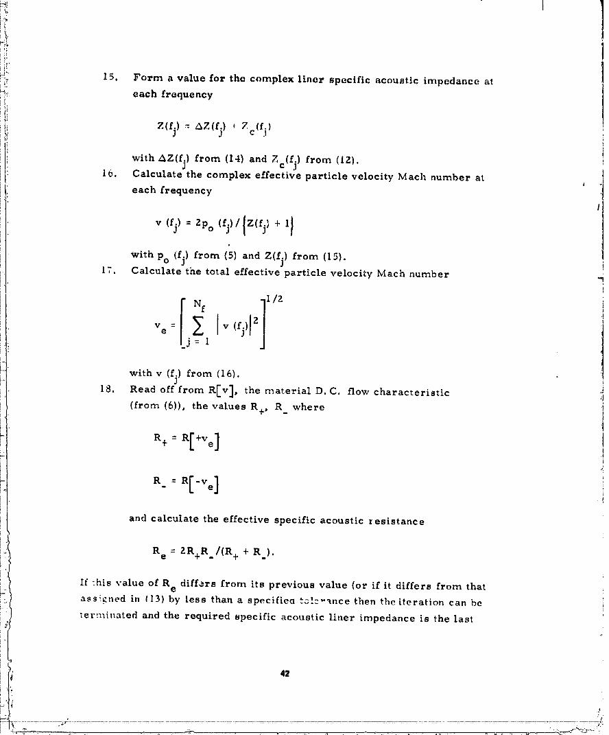
J!" 15. Form a value for the complex liner specific acoustic impedance at

_.: each frQquency

t{j. Z(fj) _ AZ(fj) ,- Z c(fjl

with AZ(fj) from (14) and Zc(f j) from (I2).16. Calculate the complex effective particle velocity Mach number at I

each frequency

v (fj) = 2po (fj)/{Z(L} + 1}

with Po (fi)_ from (5) and Z(fj) from (15), t

17. Calculate the total effective particle velocity Mach number

Nf ]1/zVe= _ [v(fj)[z

.j= I

with v (fj) from (16). it18. Read off from R[v], the material D.C. flow characteristic

(from (6)) the values R+, R where !, . ]1

R+- R[+Ve] 1tl

and calculate the effective specific acoustic xesistance

R e = ZR+R /(R+ + R ).

If "his value of R e differs from its previous value (or if it differs from that

ass!¢ned in _13) by less than a specifiea _cl=,'ance then the iteration can be

tern_inated and the required specific acoustic liner impedance is the last

_ ........ _.: .............. :9J

1976024891-TSD11

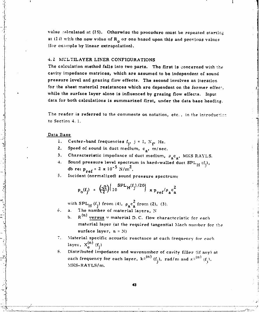
!: value ,alculated at (15). Otherwise the procedure must be repeated 8tartin_

at (14) with the new value of Re or one based upon this and previous values

(for e.-c_-ample by linear extrapolation).

4.2 MULTILAYER LINER CONFIGURATIONS

The calculation method falls into two parts. The first is concerned with :he

cavity impedance matrices, which are assumed to be independent of sound

pressure level and grazing flow effects. The second involves an iteration

.for the sheet material resistances which are dependent on the former ef._ec -,

• while the surface layer alone is influenced by grazing flow ef/ec:s. Input

data for both calculations is summarized first, under the data base heading.

The reader is referred to the comments on notation, etc., in the inrroduc:::.-

to Sectiot_ 4. 1.

Data Base

I. Center-band frequencies fj, j = I, Nf, Hz.

2. Speed of sound in duct medium, Ca, m/see.

3. Characteristic impedance of duct medium, PaCa , MHS RAYLS.

4. Sound pressure level spectrum in hard-walled duct SPL H (fj),

db re: Pref = 2 x 10 -5 N/m 2.

_. Incident (normalized) sound pressure spectrum:

po(fj) = 10 XPref/PaCa

with SPL H (fj) from (4), PaCa from (2), (3).6. a. "Ihe number of material layers, N

b. R (n} versus v material D. C. flow characteristic for each

material layer (at the required tangential ,_Iach number for the

surface layer, n = N)

7. .Xlaterial specific acoustic reactance at each frequency for each

layer, x(n)e (fj)8. Distributed impedance and wavenumber of cavity fillet" (if any) at

each frequency for each layer, k:::(n) (fj), rad/m and z ,:`_n} (fi), t.XIKS- RAY LS/m.

43

9. Cavity depth of each layer, d_:,'(n), m, if simple cavity configurations

lace (12) below).* (n)

!0. Honeycomb effective radius, r e , m, for each layer, if simple,

small-radius honeycomb forms air-filled t cavities.

11. Kinematic viscosity of cavity medium, v, m Z/see, if simple,i

small-radius honeycomb forms air-fil!ed t cavities, t

Calculation of Cavity Impedance Matrices ]

12. The cavity impedance matrices are defined by li

cos _(n) _.(n) n)]

z sin _(

A(n)(fi)= - {I/_(n)} sin _(n) cos _(n)

where

_:(n) : k ::'(n) (fj) d ::'(n), n = 1, N

{_aCa k ;:'(n)(fj)} , n= 1, N_(n) = z':'(n)(fj)/

2"he wave numbers k;_(n)(fj) and distributed impedances z:::(n)_fl/ for eachlayer, at each frequency are calculated with one or more of the methods

outlined below, as appropriate.

a. Simple air-filled cavity:

)

k ::'(n) (fj) = 2-fj/c a

or for a small-radius honeycomb cavity

Zr,f. (-f. v )112k'(n)(f.)" = _ + i

r:',:(n) cJ c ae a

and

:','(n)z _(fi) : -i(Z rf./Ca ). 3 0aCa

#i.e., if the medium in all the cavities is identical acoustically to the ductmedium, i

1976024891-TSD13

b. _J_le c avit__Lfilled wlth bulk material1' k _''n)(fj)-- and z_:_(n)(tjJ-

follow directly from (8).

Corn lex, Ioeall reactin_ng ca_ometrioa, curved liners

' +onflgurations, etc. + the matrica+ [A t '(fi)l ,hunt b+ derivedt.i

directly from meaQurement and/or theoretical models.

d. Extended reaction (nonpartitioned) liner configurations -the

impedance calculation method must be carried out in conjunc- , -

tion with the solution of the duct propagation equation, which l

provides values for kzm and m/b. In this case z ':_(n)(fj) can be

obtained from a or b above while k _:c(n)(fj) is denoted by

':<(n) (_j) and is given by (for all layers)krm

= k (f.)k'-:c(n) (_)/k a (n)rm rm j

= {(k (n)(fj)/ka)2 "6z k2zm(fj)-Sm(m/b)'_} I/2' iin=l, N

(k a : Z-fj/c a)

and k'"(n)(L) can be determined from a or b above; 5z, 5m are

unity in the absence of partitioning, but _z = 0 if the liner is

axially partitioned or 6 m = 0 if circumferentially partitioned.

Liner Impedance Calculation: Iteration for Sheet Material Acoustici Resistances

13. Choose an initial value for the material specific acoustic resistan:e

i for each sheet e. g., p

2 ';i!

415

........ : .... +..... . +.+ _..... +• + ,-..................... .......... +_;++:i+!=_ + o

1976024891-TSD14

14. Form a value for the complex material specific acoustic impedance

for each sheet at each frequency

15. Calculate the complex liner specific acoustic impedance at each ' _1

frequency by repeated application of the following equation, start- il

ingwithd°_(q):O,_(o)(_):I.0 i

/ ': )(fj) jI"1 Az(n)(L) A(n)(fJ ) _( 1

Iv(n)(5) o : dn-ll(fj_"

~(n) _

with A (n) (fj)fronl (112).(The resulting values _('_)(fi),v (fi)p(O)correspond to an arbitrary value of ' (f.) and are denoted by'tilde. ) i

) 1q

The liner specific acoustic impedance is given by

!

In. a. Calculate the actual, complex particle velocity Math number at

each frequency for the surface layer {n -- N) i.!i

"(">(_)" '_o(_?/{_(_)+'} !i

with po(fj) from (5) and z(_) from (15).

b. Calculate the actual, complex particle velocity Mach number

for all the remaining layers at each frequencyJ

{-<")(_)_1_,.,i,,(n)(q)} " \dN)(5)] (q))

with _r(Nl(fj) froth (15) and v(Nl(fj) from (16a).

,i

i

1976024891 -TSEOJ

17. Calculate the total eHective particle velocity MaCh number for each

layer

Lj=I

18. Read oft from R (n) iv] (the material D.C. flow characteristics

from (6), the sheet material specific acoustic resistances corres-

ponding to positive and negative values of the effective velocity i

Mach numbers from (17): ,Ii

i

/ ,and calculate the effective specific acoustic resistances with

(n)1£ each value R e , n = 1, N differs from its previous value (or ifeach differs from that assigned in (13) by less than a specified

tolerance then the iteration can be terminated and the required

liner specific acoustic impedance is the last value calculated at (15).

Otherwise the procedure must be repeated starting at (14)with the

newvalues "--'{R_en)I or a vector based on this and preceeding vectors

(for example, by linear extrapolation).

• I

Section 5

_ CONCLUDING REMARKS

iA natural result o£ a review is the identification o£ unanswered questions.

Many such questions could be raised as to why a material has a certain

acoustic property, but in this paper this area has been neglected, assuming

that the material property would be measured and then used to compute the

," liner property. This is a valid approach and is recommended aS the method

to be used in the future; however, it is recognized that this approach requires

both the development and standardization o£ precise measurement techniques.

In view o£ the importance of flow on material properties, it is recommended

that precision methods be developed for the measurement of the flow resistance

of materials in the presence of flow, including the _oundary layer parameters

as variables. It is also recon_rnended that methods of measuring the nonlinear

acoustic in_pedance of materials in presence of flow be developed. This impe-

dance measurement must be done using time-domain techniques to see if the

correspondence between flow resistance and acoustic resistance is retained

• valid in the presence of tangential flow.

Very little is known about the way a broadband spectrum affects the apparent

(linearized) properties o£ a material. In the present paper, an rms effective

velocity was recommet_ded because it is realized that complex spectra, or

real-time information is not generally available, it is worthwhile exploring

some of these questions by looking at the material and liner properties the

time domain, where the nonlinear effects are easier to characterize but the

geometric effects, such as liner depth_ are more complicated.

The extension of the properties of linear locally reacting liners to the case of

extended reaction is deceptively simple. It should be emphasized that this is

not possible in the case of nonlinear liners. Further research is needed on

nonlinear extended reaction liners; however, it is beyond the scope of the

present paper to discuss this in detail.

49

o_ ,,", _, o, . _ , , _ ,_, 'o , _,. t),_' " '_" _- . _° o ° . ,oo,, • ' " o o

1976024891-TSE03

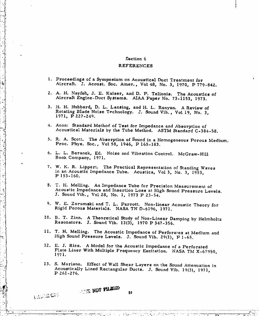
' Section 6

REFERENCES

t

1. Proceedings of a Symposium on Acoustical Duct Treatment forAircraft. J. Acoust. Soc. Amer., Vol 48, No. 3, 1970, I:' 779-842.

2. A. H. Nayfeh, J. E. Kaisers and D. P. Telionis. The Acoustics o£Aircraft Engine-Duct System_. AiAA Paper No. 73-1i53, 1973.

3. H. H. Hubbard_ D. L. Lansing, and H. L. Runyan. A Review ofRotating Blade Noise Technology. J. Sound Vib., Vol 19, No. 3,1971, P227-249.

4. Anon: Standard Method of Test for Impedance and Absorption o£Acoustical Materials by the Tube Method. ASTM Standard C-384-58.

5. R. A. Scott. The Absorption o£ Sound in a Homogeneous Porous Medium.Proc. Phys. Soc., Vol 58, i746, P 165-183.

6. L. L. Beranek, Ed. Noise and Vibration Control. McGraw-Hill

Book Company, 1971.

7. W. K. R. Lippert. The Practical Representation of Standing Wavesin an Acoustic Impedance Tube. Acustica, Vol 3, No. 3, 1953,P 153-160.

8. T. H. Melling. An Impedance Tube for Precision Measurement o£

Acoustic Impedance and Insertion Loss at High Sound Pressure Levels.J. Sound Vib., Vol 28, No. I, 1973 P 23-54.

9. W. E. Zorumski and T. L. Parrott. Non-linear Acoustic Theory for

Rigid Porous Materials. NASA TN D-6196, 1971.

10. B. T. Zinn. A Theoretical Study of Non-Linear Damping by HelmholtzResonators. J. Sound Vib. 13(3), 1970 P 347-356.

l l. T. H. Melling. The Acoustic Impedance of Perforates at Medium and

High Sound Pressure Levels. J. Sound Vib. 29(1), P 1-65.

12. E. J. Rice. A Model for the Acoustic Impedance of a PerforatedPlate Liner With Multiple Frequency Excitation. NASA TM X-67950,1971.

13. S. Mariano. Effect o£ Wall Shear Layers on the Sound Attenuation inAcoustically Lined Rectangular Ducts. J. Sou.rid Vib. 19(3), 1971,P Z61-Z76.

.............± .....

.,° .o.!!............ ,-,.. .- 1976024891-TSE04

14. E. J. Rice. A Model for the Pressure _xcitation, Spectrum and

Acoustic Impedance of Sound Absorbers in the Presence of GrazingFlow. AIAA Paper No. 73-995 and NASA TM X-7!418, 1973.

15. D. L. Armstrong. Acoustic Grazing Flow Impedance Using WaveguidePrinciples. NASA CR 120848, 1971.

16. W. Eversman0 M. D. Nelsen, D. Armstrong and O. J. Hail. Design ofAcoustic Linings for Ducts With Flow. J. Aircraft 9(8), 1972, P548-556.

17. C. Zwicker and C. W. KoSten. Sound AbSorbing MaterialS. Elsevier

Publishing Companyj New York, NY, 1949. /

18. K. W. Ingard and H. Ising. Acoustic Non-iinearity of an Orifice.3. Acoust. Soc. Amer. 42(i), 1967, P 6-17.

19. L. S. Wirt. Analysis, Testing, and Design of Ducts. J. Acoust. Soc.Amer. 51(5), 1972, P 1448-1463.

20. U. J. Kurze and C. H. Allen. Influence of Flow and High Sound Levelon the Attenuation in a Lined Duct. J. Acoust. Soc. Amer. 49(5),1971, P 1643-1654.

21. P. M. Morse and K. U. Ingard. Theoretical Acoustics. McGraw-HillBook Company, 1968.

22. E. Fader and L. W. Dean, IH. Analytical and Experimental Studiesfor Predicting Noise Attenuation in Acoustica11y Treated Ducts forTurbofan Engines. NASA CR-1373, 1969.

23. D. Ronneberger. The Acoustical Impedance of Holes in the Wall ofFlow Ducts. J. Sound Vib. 24(1), I972, P 133-150.

24. Y. Hirata and T. Itow. Influence of Air Flow on the AttenuationCharacteristics of Resonator Type Mufflers. Acoustics 28(2_, 1_73,P 77-132.

25. M. Budoff and W. E. Zorumski. Flow Resistance of Perforated Plates

in Tangential Flow. NASA TM X-2361, October 1971.

26. J. W. Posey and K. J. Compton. Effect of Nonsymmetrical FlowResistance upon Orifice impedance. NASA TM X-72624, IO74.

27. T. Rogers and A. S. Hersh. The Effect of Grazing Flow on theSteady State Resistance of Square-Edged Orifices. AIAA Paper No.75-493, March 1975.

Z8. D. L. Armstrong, R. J. Beckemeyer and R. F. Olsen. ImpedanceMeasurements of Acoustic Duct !,inerswith Grazing Flow. J. Acoust.

Soc. Amer., Vol 55, No. 6 1974.

-_ 52

J

1976024891-TSE05

29. P. D. Dean. An In Situ Method o£ Wall Acoustic Impedance Measure-ment in Flow Ducts. J. Sound Vib., Vot 33, No. 3, 1974, P 1-34.

30. L. S. Wirt. The Design of Sound Absorptive Materials to Meet• Special Requirements. Paper Presented at 86th Meeting of the

Acoustical Society o£ America, Los Angeles, California, 1973.

31. W. E. Zorumski. Acoustic Impedance of Curved Multi-Layered DuctLinerS. NASA TN D-7277, 1973.

32. D. Edkins. Acoustically Treated Ground Tests Nacelle for the GeneralElectric TF39 Turbofan. NASA CR-IZ0915, January 1972.

1976024891-TSE06