NASA Orbital Debris Engineering Model ORDEM 3.0 User’s Guide · NASA Orbital Debris Engineering...

NASA/TP-2014-217370

NASA Orbital Debris Engineering Model ORDEM 3.0 - User’s Guide Orbital Debris Program Office Eugene G. Stansbery Mark J. Matney NASA Johnson Space Center Houston, Texas Paula H. Krisko Phillip D. Anz-Meador Matthew F. Horstman John N. Opiela Eric Hillary Nicole M. Hill Robert L. Kelley Andrew B. Vavrin David R. Jarkey Jacobs Houston, Texas National Aeronautics and Space Administration Lyndon B. Johnson Space Center Houston, Texas 77058

April 2014

THE NASA STI PROGRAM OFFICE . . . IN PROFILE

Since its founding, NASA has been dedicated to the advancement of aeronautics and space science. The NASA Scientific and Technical Information (STI) Program Office plays a key part in helping NASA maintain this important role. The NASA STI Program Office is operated by Langley Research Center, the lead center for NASA’s scientific and technical information. The NASA STI Program Office provides access to the NASA STI Database, the largest collection of aeronautical and space science STI in the world. The Program Office is also NASA’s institutional mechanism for disseminating the results of its research and development activities. These results are published by NASA in the NASA STI Report Series, which includes the following report types: • TECHNICAL PUBLICATION. Reports

of completed research or a major significant phase of research that present the results of NASA programs and include extensive data or theoretical analysis. Includes compilations of significant scientific and technical data and information deemed to be of continuing reference value. NASA’s counterpart of peer-reviewed formal professional papers but has less stringent limitations on manuscript length and extent of graphic presentations.

• TECHNICAL MEMORANDUM.

Scientific and technical findings that are preliminary or of specialized interest, e.g., quick release reports, working papers, and bibliographies that contain minimal annotation. Does not contain extensive analysis.

• CONTRACTOR REPORT. Scientific

and technical findings by NASA-sponsored contractors and grantees.

• CONFERENCE PUBLICATION. Collected papers from scientific and technical conferences, symposia, seminars, or other meetings sponsored or cosponsored by NASA.

• SPECIAL PUBLICATION. Scientific,

technical, or historical information from NASA programs, projects, and mission, often concerned with subjects having substantial public interest.

• TECHNICAL TRANSLATION.

English-language translations of foreign scientific and technical material pertinent to NASA’s mission.

Specialized services that complement the STI Program Office’s diverse offerings include creating custom thesauri, building customized databases, organizing and publishing research results . . . even providing videos. For more information about the NASA STI Program Office, see the following: • Access the NASA STI Program Home

Page at http://www.sti.nasa.gov • E-mail your question via the internet to

[email protected] • Fax your question to the NASA Access

Help Desk at (301) 621-0134 • Telephone the NASA Access Help Desk

at (301) 621-0390 • Write to: NASA Access Help Desk NASA Center for AeroSpace

Information 7115 Standard Hanover, MD 21076-1320

NASA/TP-2014-217370

NASA Orbital Debris Engineering Model ORDEM 3.0 - User’s Guide Orbital Debris Program Office Eugene G. Stansbery Mark J. Matney NASA Johnson Space Center Houston, Texas Paula H. Krisko Phillip D. Anz-Meador Matthew F. Horstman John N. Opiela Eric Hillary Nicole M. Hill Robert L. Kelley Andrew B. Vavrin David R. Jarkey Jacobs Houston, Texas National Aeronautics and Space Administration Lyndon B. Johnson Space Center Houston, Texas 77058

April 2014

Acknowledgements We would like to thank Debi Shoots and Vladenka Oliva for editing this document. The development team thankfully acknowledges the careful review and detailed comments and suggestions provided by the software beta review panel.

Available from:

NASA Center for AeroSpace Information National Technical Information Service 7115 Standard Drive 5285 Port Royal Road Hanover, MD 21076-1320 Springfield, VA 22161 301-621-0390 703-605-6000

This report is also available in electronic form at http://ston.jsc.nasa.gov/collections/TRS/

i

ORDEM 3.0 Team NASA: Edwin S. Barker Jer-Chyi Liou Mark J. Matney Eugene G. Stansbery Jacobs: Kira J. Abercromby Phillip D. Anz-Meador Jon S. Berndt Heather M. Cowardin Nicole M. Hill Eric Hillary Matthew F. Horstman David R. Jarkey Kandy S. Jarvis Robert L. Kelley Paula H. Krisko Mark K. Mulrooney John N. Opiela Christopher L. Stokely Andrew B. Vavrin David O. Whitlock Yu-Lin Xu

ii

Contents

Acronyms ......................................................................................................................v Symbols .................................................................................................................... vi 1.0 Introduction ...................................................................................................................1

1.1 Requirements of an Orbital Debris Engineering Model .......................................1 1.2 Limitations of an Orbital Debris Engineering Model ...........................................2 1.3 A Historical Overview of Orbital Debris Engineering Models ............................2 1.4 Point of Contact ....................................................................................................3

2.0 ORDEM 3.0 Model ......................................................................................................4

2.1 Software Installation and Removal .......................................................................7 2.2 Software Description ............................................................................................9 2.3 Program Execution..............................................................................................10

2.3.1 GUI-based Computation .........................................................................10 2.3.2 Command-line-based Computation ........................................................16

2.4 Output Data and Graphs ......................................................................................17 2.4.1 Spacecraft Mode Graphs .........................................................................21 2.4.2 Telescope/Radar Mode Graphs ...............................................................26

3.0 References ...................................................................................................................29 Appendix A ORDEM 3.0 Processor Messages and GUI Dialog Boxes ..................... A-1 Appendix B ORDEM 3.0 Input/Output File Formats ..................................................B-1

B.1 Input File Format .....................................................................................B-1 B.2 Output File Formats .................................................................................B-3

B.2.1 SIZEFLUX_SC.OUT............................................................................B-3 B.2.2 VELFLUX_SC.OUT ............................................................................B-4 B.2.3 BFLY_SC.OUT ....................................................................................B-4 B.2.4 DIRFLUX_SC.OUT .............................................................................B-5 B.2.5 IGLOOFLUX_SC.OUT........................................................................B-7 B.2.6 IGLOOFLUX_SIGMAPOP_SC.OUT .................................................B-9 B.2.7 IGLOOFLUX_SIGMARAN_SC.OUT ................................................B-9 B.2.8 FLUX_TEL.OUT..................................................................................B-9 B.2.9 IGLOOFLUX_TEL.OUT ...................................................................B-10 B.2.10 IGLOOFLUX_SIGMAPOP_TEL.OUT .............................................B-10 B.2.11 IGLOOFLUX_SIGMARAN_TEL.OUT ............................................B-10

Appendix C How to Use Uncertainty Files ..................................................................C-1 Appendix D ORDEM 3.0 Current Runtime Estimates ................................................ D-1

D.1 Runtime Estimates for Spacecraft Assessment Mode ............................ D-1 D.2 Runtime Estimates for Telescope/Radar Assessment Mode .................. D-1

iii

Figures 2-1 ORDEM GUI options and coding structure flowchart. .........................................11 2-2 ORDEM 3.0 project window. ................................................................................12 2-3 ORDEM 3.0 Spacecraft Assessment window .......................................................14 2-4 ORDEM 3.0 Spacecraft Assessment TLE window ...............................................15 2-5 ORDEM 3.0 Telescope/Radar Assessment window .............................................16 2-6 ORDEM 3.0 graph options menu ..........................................................................18 2-7 ORDEM 3.0 graph export dialog window .............................................................19 2-8 ORDEM 3.0 graph configuration dialog window ..................................................19 2-9 ORDEM 3.0 Spacecraft Assessment Graph selection window .............................21 2-10 Spacecraft Assessment Average Flux vs. Size graph ............................................22 2-11 Spacecraft Assessment Flux Calculator. ................................................................23 2-12 Spacecraft Assessment skyline butterfly graph ....................................................24 2-13 Spacecraft Assessment radial butterfly graph ........................................................24 2-14 Spacecraft Assessment Velocity flux distribution .................................................25 2-15 Spacecraft Assessment 2-D Directional Flux projection .......................................25 2-16 ORDEM 3.0 Telescope/Radar Assessment Graph selection window ...................26 2-17 Telescope/Radar Assessment Flux vs. Altitude graph, LEO region-only. ............26 2-18 Telescope/Radar Assessment Flux vs. Altitude graph, GEO region-only. ............27 2-19 Warning message in status window in both Spacecraft and Telescope/Radar

modes for analysis apogees above 2000 km ..........................................................28 A-1 Low perigee error ................................................................................................ A-5 A-2 High perigee warning .......................................................................................... A-5 A-3 Low apogee error.. .............................................................................................. A-5 A-4 High apogee warning .......................................................................................... A-6 A-5 Switched apogee and perigee error ..................................................................... A-6 A-6 Low semi-major axis error .................................................................................. A-6 A-7 Out-of-range ECC error ...................................................................................... A-7 A-8 Out-of-range INC error ....................................................................................... A-7 A-9 Out-of-range AP error ......................................................................................... A-7 A-10 Out-of-range RAAN error ................................................................................... A-8 A-11 Out-of-range latitude error .................................................................................. A-8 A-12 Out-of-range azimuth error ................................................................................. A-8 A-13 Out-of-range elevation ........................................................................................ A-9 A-14 Out-of-range flux calculator size ........................................................................ A-9

iv

Tables 2-1 Feature Comparison of ORDEM 2.0 and ORDEM 3.0 ...........................................5 2-2 Contributing Data Sets .............................................................................................6 2-3 Contributing Models (with Corroborative Data) .....................................................6 2-4 Input File Population Bins for LEO to GTO ...........................................................6 2-5 Input File Population Bins for GEO ........................................................................7 2-6 Files in Application Directory ...............................................................................10 2-7 Files in Project Directory .......................................................................................10 2-8 Advanced Project Options .....................................................................................13 2-9 Files Output by Each ORDEM 3.0 Mode ..............................................................20 A-1 Processor Messages ............................................................................................ A-1 B-1 The ORDEM 3.0 Input File, “ORDEM.IN” ........................................................B-2 B-2 Files Output by ORDEM 3.0 Modes ...................................................................B-3 B-3 Illustration of Output for SIZEFLUX_SC.OUT ..................................................B-4 B-4 Illustration of Output for VELFLUX_SC.OUT...................................................B-4 B-5 Illustration of Output for BFLY_SC.OUT...........................................................B-5 B-6 Illustration of Output for DIRFLUX_SC.OUT ...................................................B-6 B-7 Illustration of Output for IGLOOFLUX_SC.OUT ..............................................B-8 B-8 Illustration of Output for FLUX_TEL.OUT ........................................................B-9 B-9 Illustration of Output for IGLOOFLUX_TEL.OUT .........................................B-11

v

Acronyms

2-D .................................................... two dimensional

CPU ................................................... Central Processing Unit

FY-1C ............................................... Fengyun 1-C

GEO .................................................. Geosynchronous Orbit

GOST ................................................ GOsudarstvennyy STandart

GTO .................................................. Geosynchronous Transfer Orbit

GUI ................................................... graphical user interface

HAX .................................................. Haystack AuXiliary radar

HVIT ................................................. (NASA) Hypervelocity Impact Technology (Group)

ISS ..................................................... International Space Station

LEGEND ........................................... LEO-to-GEO Environment Debris Model

LEO ................................................... low Earth orbit

MASTER .......................................... Meteoroid and Space Debris Terrestrial Environment Reference

MODEST .......................................... Michigan Orbital Debris Survey Telescope

NaK ................................................... Sodium potassium eutectic coolant for RORSAT reactors

NASA ................................................ National Aeronautics and Space Administration

ODPO ................................................ (NASA) Orbital Debris Program Office

ORDEM ............................................ Orbital Debris Engineering Model

RAM ................................................. random-access memory

RAAN ............................................... right ascension of the ascending node

RORSAT ........................................... Radar Ocean Reconnaissance SATellite

SBRAM ............................................. (NASA ODPO) Satellite Breakup Risk-Assessment Model

S/C ..................................................... spacecraft

SOCIT ............................................... Satellite Orbital Debris Characterization Impact Test

SSN ................................................... Space Surveillance Network

STS .................................................... Space Transportation System

SUA ................................................... Software Usage Agreement

TLE ................................................... Two-Line Element

vi

Symbols

a ....................................................... semi-major axis

AP, ............................................... argument of perigee

az ...................................................... azimuth

ECC, e .............................................. eccentricity

el ...................................................... elevation

ha ...................................................... apogee altitude

hp ...................................................... perigee altitude

INC, i ............................................... inclination

MM, n .............................................. mean motion

RAAN ......................................... right ascension of the ascending node

σ ....................................................... standard deviation

vr ...................................................... relative velocity

1

1.0 Introduction

This National Aeronautics and Space Administration (NASA) Orbital Debris Engineering Model (ORDEM) 3.0 User’s Guide accompanies delivery of the latest upgraded Orbital Debris Engineering Model (ORDEM 3.0). The user’s guide also provides a top-level program description and a list of capabilities. It includes appendixes with descriptions of runtime error and information codes (Appendix A), descriptions of input/output file formats (Appendix B), how to use uncertainty files (Appendix C), and descriptions of typical runtimes for different orbit configurations (Appendix D). Another document, the ORDEM 3.0 Technical Document, will be released later. It will contain a detailed description of the program (finite element model, coding structure, and applications), an overview of all data measurement sources, a data analysis section that describes the use of those data sources, and a description of statistical tools, theory, and model data. ORDEM 3.0 supersedes the previous NASA Orbital Debris Program Office (ODPO) model – ORDEM2000 (Liou, et al. 2002). The availability of new sensor and in situ data, the re-analysis of older data, and the development of new analytical techniques has enabled the construction of this more comprehensive and sophisticated model. An upgraded graphical user interface (GUI) is integrated with the software. This upgraded GUI uses project-oriented organization and provides the user with graphical representations of numerous output data products. These range, for example, from the conventional average debris size (or altitude bin) vs. flux for chosen analysis orbits (or views) to the more complex color-contoured, two-dimensional (2-D) directional flux diagrams in local spacecraft elevation and azimuth. Finally, the sequential numbering scheme has been adopted to sever upgrades from simple calendar accounting and to emphasize major advances in the model design and supporting data analysis. Also this scheme will allow for quicker interim model upgrades than have previously been accomplished. The current model is ORDEM 3.0. This permits the older models ORDEM96 and ORDEM2000 to be retroactively referred to as ORDEM 1.0 and ORDEM 2.0, respectively.

1.1 Requirements of an Orbital Debris Engineering Model

The primary requirement for any engineering model is to provide the user with accurate results expediently. The two main types of ORDEM users are spacecraft designers and operators, and debris researchers. (A third user group includes mission planners and analysts using the ODPO Debris Assessment Software package, which implements ORDEM populations in calculations for spacecraft damage probability.) The requirements of each user group differ somewhat, though they share many common requirements. To facilitate implementation of cost-effective shielding, the designer of an oriented spacecraft requires detailed estimates of the particle flux as a function of local azimuth/elevation. (Such detail is not required for a randomly tumbling spacecraft.) To determine this flux accurately, the user must carefully assess the debris size and orbit

2

distribution. Because of the long lead times in new satellite designs, the temporal behavior of the debris environment over a satellite’s lifetime is also important. When an observer is planning a debris observation campaign, predicted fluxes are used to ensure that the experiment planning and design can accommodate the quantity and rate of data collection. Ultimately, measurements will be compared to the model predictions and will be the final figure of merit of the model’s veracity. Predicted fluxes will depend upon the inclination and altitude distribution of resident space objects visible from the ground-based sensor location. Additionally, an observer must consider whether the sensor is fixed in its orientation or is steerable in azimuth and elevation. When bistatic radars use parallax, the altitude distribution becomes crucially important due to common field-of-view constraints. Thus, any such model must include, at a minimum, an accurate assessment of the orbital debris environment as a function of altitude, latitude, and debris size. ORDEM 3.0 is an engineering model that is consistent with this requirement. It is based on debris populations with various altitude, inclination, and size distributions. The model provides a complete description of the environment, including debris flux, onto spacecraft surfaces or the debris detection rate observed by a ground-based sensor.

1.2 Limitations of an Orbital Debris Engineering Model

Some studies are beyond the scope of the ORDEM series. For example, the series cannot reliably evaluate the short-term collision risk between fragments from recent breakup events and an orbiting satellite. Such an assessment requires highly accurate orbital positioning and propagation – a task that the NASA ODPO Satellite Breakup Risk-Assessment Model (SBRAM) accomplishes. The long-term impact of various mitigation measures on the debris environment must rely on a debris evolution model that includes effects such as the solar activity cycle (affecting atmospheric density and hence the decay rate of objects in low Earth orbit [LEO]), the growth of the space vehicle population, and a projected fragmentation rate. The NASA ODPO LEO-to-GEO Environment Debris Model (LEGEND) is applicable for examining the consequences of such phenomena.

1.3 A Historical Overview of Orbital Debris Engineering Models

The first debris engineering model was developed for the Space Station Program Office in 1984 (Kessler 1984). Later models were assembled for the Strategic Defense Initiative Organization, for various LEO spacecraft programs (Kessler 1989), and for the Space Station Program Office (Kessler 1991). Each of these portrayed the environment as curve fits to describe the distributions of large objects (the Space Surveillance Network [SSN] – a catalog of objects larger than approximately 10 cm) and small objects (as recorded by the inspection of surfaces exposed to and returned from space). Both periodic (solar cycle) and secular (launch traffic and fragmentation growth rate) effects were included explicitly. A significant requirement of these models was that they be easily executed by a programmable calculator or be capable of manual manipulation within a reasonable time.

3

The need to better define the debris environment eventually outgrew this latter requirement. ORDEM 1.0, formerly ORDEM96, (Kessler 1996) was the first model that required a personal computer for effective implementation. ORDEM 1.0 pioneered the use of debris population ensembles characterized by altitude, eccentricity, inclination, and size. ORDEM 2.0, formerly ORDEM2000, (Liou, et al. 2002) adopted a similar approach, but it replaced the final remnants of curve fitting, as used by all previous NASA engineering models, with a finite element model to represent the debris environment. Engineering models are not limited to the NASA models mentioned above. For example, the European Space Agency Meteoroid and Space Debris Terrestrial Environment Reference (MASTER) (Sdunnus 2001) series of models performs similar functions, as did the former Soviet Union’s three-population (orbital debris, micrometeoroids, and “Earth-orbiting meteoroids”) GOST (GOsudarstvennyy STandart – meaning state standard) engineering model. MASTER-2005 and MASTER-2009 (Oswald 2006) and (Flegel, et al. 2010) are similar to the latest in the ORDEM series of models (ORDEM 2.0 and ORDEM 3.0), whereas the Soviet model is similar to the earlier NASA models.

1.4 Point of Contact

The official point of contact for ORDEM 3.0 at the NASA ODPO is: Mr. Gene Stansbery, ODPO Program Manager Mail Code: KX NASA Johnson Space Center Houston, TX 77058 USA Phone: (281) 483-8417 Email: [email protected]

4

2.0 ORDEM 3.0 Model

Since ORDEM 2.0 was released, new debris data have become available and analysis techniques have matured to more currently reflect the debris environment. Based on these data and techniques, NASA established a number of mandates for the new engineering model, ORDEM 3.0. With the singular events that occurred near the end of the last decade (Fengyun-1C [FY-1C] anti-satellite test and Iridium/Cosmos collisions), the mandates for ORDEM 3.0 have expanded to:

extend the model to geosynchronous orbit (GEO) with the addition of Michigan Orbital Debris Survey Telescope (MODEST) data and modeling techniques to include GEO objects down to 10 cm,

investigate and account for Molniya-type orbits with fixed arguments of perigee,

continue to include radar detections of debris (SSN, Haystack AuXiliary radar [HAX], Haystack, and Goldstone) in the model and make use of these larger data sets to apply model fiducial points at half-decade sizes,

use the NASA Hypervelocity Impact Technology (HVIT) group’s Space Transportation System (STS) microdebris impact database (STS 71-135 listing over 600 impacts), which includes crater dimension, chemical composition, and derived damage equations on STS aluminum radiator panels and windows,

assign small fragment (<10 cm) material density based on the Satellite Orbital Debris Characterization Impact Test (SOCIT) laboratory impact test results and on-orbit STS returned surface impactor analysis,

model the Radar Ocean Reconnaissance SATellite (RORSAT) sodium potassium (NaK) coolant droplet population with radar measurements,

include specific, major debris-producing events that have been thoroughly observed (i.e., the remnants of the FY-1C on 11 January 2007, and the accidental collision of Iridium 33 and Cosmos 2251 on 10 February 2009) and add to the general population,

include long-term, debris-producing events that have been surmised from LEO high-altitude radar data (i.e., SNAPSHOT, Transit, and 56° inclination-debris shedding activity) and add to the general population,

fully develop the Bayesian statistical model for population derivation,

include debris population uncertainties,

provide “igloos” with equal-angle elements for full surrounding visualization of debris flux on spacecraft, and

build the ORDEM 3.0 GUI to accommodate the full-angle views (i.e. 4 steradian views) of the large yearly input files.

Table 2-1 compares ORDEM 3.0 top-level output features to those of ORDEM 2.0. These are detailed in output file formats and graphics in Section 2.4 and Appendix B. The new model

5

input populations are pre-derived directly from the data sources listed in Table 2-2. These consist of in-situ sources, for debris ranging from 10 m to less than 1 mm, and remote sensors, for debris ranging from 1 mm to over 1 m. These data are applied to ORDEM 3.0 in a maximum likelihood estimation and a Bayesian statistical process, respectively, in which the NASA ODPO models listed in Table 2-3 form the a priori conditions. Those modeled debris populations are reweighted in number to be compatible with the data in orbital regions where the data are collected. By extension, model debris populations are reweighted in regions where no data are available (e.g., all sizes in low latitudes and sub-millimeter sizes at altitudes above the International Space Station [ISS]).

Table 2-1: Feature Comparison of ORDEM 2.0 and ORDEM 3.0

Parameter ORDEM 2.0 ORDEM 3.0 Spacecraft & Telescope/Radar analysis modes

Yes Yes

Time range 1991 to 2030 2010 to 2035

Altitude range with minimum debris size

200 to 2000 km (>10 m) (LEO )

100 to 40,000 km (>10 m)* (LEO to GTO) 34,000 to 40,000 km (>10 cm) (GEO)

Orbit types Circular (radial velocity ignored)

Circular to highly elliptical

Model population breakdown by type & material density

No

Intacts Low-density (1.4 g/cc) fragments Medium-density (2.8 g/cc)

fragments & microdebris High-density (7.9 g/cc)

fragments & microdebris RORSAT NaK coolant droplets (0.9 g/cc)

Model cumulative size thresholds (fiducial points)

10 m, 100 m, 1 mm, 1 cm , 10 cm, 1 m

10 m, 31.6 m, 100 m, 316 m, 1 mm, 3.16 mm, 1 cm, 3.16 cm, 10 cm, 31.6 cm, 1 m

Flux uncertainties No Yes Total input file size 13.5 MB 1.25 GB Meteoroids No No** *While the geosynchronous transfer orbit (GTO) is not as well observed as LEO, the orbital

dynamic forces and mechanisms for fragmentation are considered to be similar. The ODPO therefore allows for > 10 m fluxes through GTO. For GEO the dynamics (including perturbation forces and impact velocities) as well as the size and structure of satellites are unique, though GTO and GEO physically overlap. The ODPO provides GEO debris fluxes for 10 cm and larger only. This is based on the SSN (1 m and larger), the MODEST uncorrelated target data (30 cm – 1 m) and the MODEST uncorrelated targets extended to 10 cm. Any fluxes below that 10 cm threshold at altitudes above LEO altitudes are solely due to GTO objects.

**The ODPO has decided that the meteoroid environment will not be included in ORDEM. The user must include a separate meteoroid model to create the total space debris environment.

6

Table 2-2: Contributing Data Sets

Observational Data Role Region/Approximate Size SSN catalog (radars, telescopes) Intacts & large fragments LEO > 10 cm, GEO > 1 m HAX (radar) Statistical populations LEO > 3 cm Haystack (radar) Statistical populations LEO > 5.5 mm Goldstone (radar) Statistical populations 2 mm < LEO < 8 mm STS windows & radiators (returned surfaces)

Statistical populations 10 m < LEO < 1 mm

MODEST (telescope) GEO data set GEO > 30 cm

Table 2-3: Contributing Models (with Corroborative Data)

Model Usage Corroborative Data LEGEND LEO Fragments > 1 mm

GEO Fragments > 10 cm SSN, Haystack, HAX, MODEST, SSN

Degradation/Ejecta 10 m < LEO < 1 mm STS windows & radiators

The ORDEM 3.0 input debris populations are binned in the quasi-orthogonal orbital elements in Table 2-4 for non-GEO objects and in Table 2-5 for GEO objects. Bin sizes are chosen to complement actual population distributions. The final files are from the direct yearly input database of ORDEM 3.0. The binned input populations are accessed via the Spacecraft and Telescope/Radar modes; where the former uses the encounter igloo method and the later uses a segmented bore-sight vector for computation of flux. This process is described more fully in the following sections and will be discussed in depth in the ORDEM 3.0 Technical Document.

Table 2-4: Input File Population Bins for LEO to GTO

Parameter Binning Intervals Total No. of Bins

Perigee altitude, hp 100 ≤ hp < 2000 km → 33.33 km bins

2000 ≤ hp < 10,000 km → 100 km bins 10,000 ≤ hp < 40,000 km → 200 km bins

287

Eccentricity, e 0 ≤ √e < 0.02666 → 0.02666 bin 0.02666 ≤ √e < 1 → 0.01333 bins

74

Inclination, i 0° ≤ i < 180° → 0.75° bins 240

7

Table 2-5: Input File Population Bins for GEO

Parameter Binning Intervals Total No. of Bins

Mean Motion, n 0.5 ≤ n < 0.95 → 0.01 rev/day bins 0.95≤ n < 1.05 → 0.001 rev/day bins 1.05≤ n < 1.80 → 0.01 rev/day bins

220

Eccentricity, e 0 ≤ √e < 0.5 → 0.02 bins 25

Inclination, i 0° ≤ i < 0.2° → 0.2° bins

0.2° ≤ i < 1.0° → 0.8° bins 1° ≤ i < 25° → 1° bins

26

Right ascension of ascending node,

0° ≤ < 360° → 5° bins 72

2.1 Software Installation and Removal

The minimum system requirements to install ORDEM 3.0 are listed below:

Microsoft Windows XP or later Microsoft .Net framework 4.0 or greater 512 MB random-access memory (RAM) 1.5 GB available disk space

NOTE: Depending on user inputs, ORDEM 3.0 runtimes will vary from 10 minutes (for low LEO circular orbits) to over 6 hours (for high apogee GTO orbits). A faster Central Processing Unit (CPU) will reduce runtime, but the computational method cannot take advantage of multiple CPUs/cores.

ORDEM 3.0 is distributed using an executable setup file. The setup will install the program’s executable files and all necessary support files within the appropriate directories. To install the ORDEM 3.0 software, follow the procedure below:

1. If not already installed, obtain and install the Microsoft .NET framework 4.0 or greater (http://www.microsoft.com/net/Download.aspx).

2. Obtain the installation file for ORDEM 3.0 (ORDEM3.0_Install.exe) from the NASA ODPO Point of Contact.

3. Run the ORDEM 3.0 installer. This may require special user privileges (i.e., Administrator) depending on the computer’s security settings.

The installer will set up the ORDEM 3.0 software, libraries, and extensive data files. The installer will also create Windows-based shortcuts to the ORDEM 3.0 GUI, User’s Guide, and software uninstaller. By default, the shortcuts are located in the Windows-based Start menu under Programs ORDEM 3.0.

8

Use the following steps to install the program:

1. If the installer detects that ORDEM 3.0 is already installed, it prompts the user to remove the installed version.

2. The Welcome window verifies that the installation of ORDEM 3.0 is desired. If not, select cancel.

3. The Software Usage Agreement verifies that the user agrees to accept the software license. The user may cancel the installation or may agree and proceed to the next step.

4. The Choose Users window allows the user to select whether to install ORDEM 3.0 for all users or for the current user only.

5. Choose Install Location defines the location where the application will be installed. The default location is the “Program Files (x86)” directory. A “Browse” button will enable the user to view the file structure to define a preferred location.

6. Choose Start Menu Folder defines a folder within the Windows-based StartProgram list where the application shortcuts will appear. The default setup will be provided, but another name can be defined or an existing program folder can be selected where this application will be loaded. Click “Next” to continue with installation.

7. The Installing ORDEM 3.0 window is displayed. The progress bar displays information on the installation progress.

8. Setup Complete notifies the user that the setup has been completed and the system will not require rebooting. The user has the option to create a desktop shortcut to the ORDEM 3.0 GUI and to view the README.txt file.

9. If needed, verify that the installer added the NASA\ORDEM 3.0\model directory to the PATH environment variable.

a. To verify PATH, right-click on My Computer, then select Properties Advanced System Settings Environment Variables. In the System Variables window, select the PATH option in the System Variables list and click the “Edit” button.

b. If the NASA\ORDEM 3.0\model folder is not found in the PATH environment variable, the user can manually add this folder to PATH by typing the following in a command window:

set PATH=<path-to-ORDEM3.0>\NASA\ORDEM 3.0\model;%PATH%

Do not remove or rename files and directories installed with ORDEM 3.0. Do not modify files within the ORDEM data directory (“ORDEM 3.0\data\”). Files and directories may be

9

copied to another location if necessary, but ORDEM 3.0 requires the originally installed files to remain unaltered. Removal: ORDEM 3.0 includes an automatic removal (“un-installer”) feature. To remove ORDEM 3.0, run the program “ORDEM 3.0-uninstall.exe”, located in the “uninstall” folder of the ORDEM 3.0 application directory. This may require special user privileges depending on the computer’s security settings. A shortcut to this uninstaller in the ORDEM 3.0 program group is in the Windows Start Menu. You will need to delete manually any ORDEM 3.0 project directories that the user created. Note for Windows 7 Users: Do not attempt to uninstall ORDEM 3.0 from the “Programs and Features” portion of the Windows Control Panel; it will not work. Instead, use the above removal procedure.

2.2 Software Description

ORDEM 3.0 includes two programs: a command-line executable, which performs the numerical computations; and a separate GUI. Upon installation, these executables are stored in the Application Directory (see Table 2-6). The default location of the Application Directory is the NASA\ORDEM 3.0 folder in the “Program Files (x86)” directory. This directory also includes the debris population files that form the database of the model (stored in the subdirectory “data”). The results of an ORDEM 3.0 computation are stored in the user-defined “Project Directory”. This directory is located where the user creates it. It is a writable area for running the computational model and saving all GUI values. The user may create as many project directories as desired. The directory (shown in Table 2-7) contains the input parameter file and all output files.

10

Table 2-6: Files in Application Directory

File Name Description

data/YYYY.POP data/*.SIG data/*.TIG data/*.DAT data/*.BIN data/*.out

Yearly input population data for ORDEM 3.0 calculations Spacecraft-mode igloo description files Telescope/Radar-mode igloo description files Data defining the bin boundaries of the debris populations Binary file containing 7-dimensional Sobol sequences Gridline coordinates for the spacecraft-mode plot of “2-D Directional Flux”

help/ORDEM_UserGuide.pdf User’s guide for ORDEM 3.0

model/ORDEM.exe Computational model executable

uninstall/ORDEM_3.0-uninstall.exe Uninstall model executable

LICENSE.txt Software Usage Agreement (SUA)

ORDEM-GUI.exe Graphical user interface executable

README.txt

Table 2-7: Files in Project Directory


ORDEM-Project.prj The saved project values from the GUI

ORDEM-GUI_Log.txt The project log file

runtime.log An error log created by the command-line program

ORDEM.IN The command file, which holds the parameters for running the computational model executable

*_SC.OUT Spacecraft assessment output files

*_TEL.OUT Telescope/Radar assessment output files

* See Appendix B (Table B-2) for output file names.

2.3 Program Execution

ORDEM 3.0 may be run using the GUI or the command-line (“DOS”) interface. The GUI accepts inputs from the user, sets up and performs a single run, and displays the results as on-screen plots. The command-line interface requires the user to supply a separate text input file or a driver/batch code for serial batch processing. This interface also produces the standard output files listed in Table 2-7, but does not produce plots.

2.3.1 GUI-based Computation

The usual means of running ORDEM 3.0 is through the GUI. Figure 2-1 illustrates the user actions and subsequent program performance associated with the GUI. After mode selection, with required inputs, the ORDEM 3.0 code selects the appropriate population bin set and begins

11

the mapping of bins to encounter igloos or segmented bore-sight vectors. Encountered fluxes are compiled and tabulated in output files that are, in turn, accessed by TeeChart plotting routines via the GUI.

Figure 2-1: ORDEM GUI options and coding structure flowchart. Both LEO and GEO calculations are accessed for any orbits whose parameters overlap into LEO and GEO igloo bins. Red indicates GUI user selections;

gray background indicates ORDEM processes. Specifically, to run ORDEM 3.0 through the GUI the user chooses the “ORDEM-GUI.exe” in the Application Directory. The ORDEM 3.0 initial “project window” appears (see Figure 2-2). The user defines a project directory (the location the user chooses), to which all output files and

12

GUI settings will be saved. Project folders allow a user to save and load different projects without having to re-enter the inputs.

Figure 2-2: ORDEM 3.0 project window. The top area of the project window displays the currently selected project directory. This directory is the location for all the computational output and GUI settings. The application allows the user to save as many projects as desired. Note that creating a project directory by other means will NOT create the required “.prj” file, causing ORDEM 3.0 to reject that directory. Click the Project Directory… button to open the Project Directory selection window. To open a previously created project, the user selects the desired directory. To create a new project, the user selects the Make New Folder button in the selected directory. When the desired projected directory is selected, the user clicks the OK button. On the main project window, the current values in the GUI are saved to the current .prj file. The Reset to Defaults button resets all the GUI values to the last saved values. Toward the center of the window is a box with a list of project files in the current project directory. (If the directory is new, it is empty and the box is empty.) It provides a quick access and view to any of the files. If double clicked, a file will be opened in another window for

13

viewing. View Log will bring up a window allowing the user to view the log of past activity. Last, the Reset to Defaults button will reset all the GUI values to default values. This includes the currently known project directory in the project window and the system registry (used for loading the last used project on startup). Before moving to one of the assessment modes, Spacecraft or Telescope/Radar, the user may choose from a set encounter igloo or segmented bore-sight vector gradations in the Advanced Project Options box (see Table 2-8).

Table 2-8: Advanced Project Options

Selection Name Description

Spacecraft Igloo Bin Sizes

IGLOO_10x10x1.SIG* Spacecraft encompassing igloo with dimensions 10o in azimuth, 10o elevation, 1 km/sec in velocity

IGLOO_30x30x2.SIG Spacecraft encompassing igloo with dimensions 30o in azimuth, 30o elevation, 2 km/sec in velocity

Telescope/Radar Igloo Bin Sizes

ALT_50.TIG* ALT_100.TIG

Segmented bore-sight vector defined by 50 km or 100 km altitude bins from LEO to GEO (200 km - 40,000 km)

ALT_5_GEO.TIG ALT_50_GEO.TIG ALT_100_GEO.TIG

Segmented bore-sight vector defined by 5 km, 50 km, or 100 km altitude bins in GEO-only (34,000 km - 40,000 km)

ALT_5_LEO.TIG ALT_50_LEO.TIG ALT_100_LEO.TIG

Segmented bore-sight vector defined by 5 km, 50 km, or 100 km altitude bins in LEO-only (200 km - 2,000 km)

*The finer gradations are the ORDEM 3.0 default values (see Figure 2-2). These are recommended for any serious analysis.

2.3.1.1 Spacecraft Assessment

The Spacecraft Assessment window (see Figure 2-3) is used for evaluating the orbital debris environment for spacecraft and missions. This window contains the input fields (at the top) and the runtime output window (at the bottom).

14

Figure 2-3: ORDEM 3.0 Spacecraft Assessment window. The input orbit information can be entered as orbital parameters (hp, ha), Keplerian orbit elements (a, e), or as a standard two-line element (TLE) set. When entering input information by hand, the user can define the orbit by inclination and either the perigee and apogee altitudes or by the semi-major axis and eccentricity. The user may define the argument of perigee and right ascension of the ascending node (RAAN). It is also possible to choose a “randomized” value for argument of perigee and RAAN. The results will represent time-averaged fluxes over all possible values of the RAAN that are appropriate for long-term flux calculations in many cases. Note that a non-random choice of argument of perigee or RAAN affects only flux calculations in the Molniya-type orbits or the GEO regime, respectively. The LEO populations are assumed to consist of populations with randomized argument of perigee and RAAN, so a specific choice of these orbital elements will not affect LEO fluxes. To input the orbit as a TLE set, click on the Load from TLE button. Figure 2-4 shows the pop-up window that is displayed for decomposing a TLE.

15

Figure 2-4: ORDEM 3.0 Spacecraft Assessment TLE window.

The TLE window allows the user to specify the TLE by loading from a text file, hand typing, or pasting into the TLE area. When loading from a text file (Load from File button), the software reads only the first TLE set. The Calculate button will break down the TLE into the various orbital parameters. If these are the desired values, the user must click the Accept button. The TLE breakdown values will then appear in the Spacecraft assessment window. The Cancel button will close this window and the Clear button will clear the TLE area. After all input parameters are set in the Spacecraft assessment window, the user must click the Start button to begin the computations. The Stop button is provided to abort a run. Immediately below the Start and Stop buttons is the ORDEM 3.0 Model Output area (See Figure 2-3). After clicking the Start button, the model process will begin and the output messages will be redirected into this output area. Normal output messages from the model will appear in black text and error messages will appear in red text. The GUI will write other informative messages in blue text. (Note that the different-colored messages may not appear to be synchronized, because they come from different sources.) After running the computational model, the files listed in the “Output File" area may be viewed by clicking the icon to the right of the file name. The user can view four types of output graphs by clicking the Graphs button: average flux vs. size, directional flux “butterfly,” 2-D directional flux , and flux velocity distribution (as shown in Figure 2-9). The full description of these graphs is in Section 2.4.

16

2.3.1.2 Telescope/Radar Assessment

The Telescope and Radar Assessment window is provided for modeling the orbital debris environment as viewed through the bore-sight of a ground-based telescope or radar. Figure 2-5 shows the Telescope/Radar Assessment window.

Figure 2-5: ORDEM 3.0 Telescope/Radar Assessment window.

This window is very similar in functionality to the Spacecraft Assessment window. There are fields for the inputs, start and stop buttons for running the model, and buttons for viewing the output. There is a single output file listing Flux vs. Altitude: LEO-only, LEO+GEO, and GEO-only. This file may be viewed by clicking the icon to the right of the file name – the Graphs… button. Section 2.4 includes the full description of these graphs.

2.3.2 Command-line-based Computation

The second method of running ORDEM 3.0 is via the command-line interface, with or without a batch file. This approach is possible because the computational model is a separate executable program. Running from the command line requires the user to manually edit the ORDEM.IN

17

input file. A sample ORDEM.IN file is displayed in Table B-1. In GUI runs, this file is produced from the user set input parameters. It holds all values needed to run the simulation. The file is annotated to assist in editing if needed (the user may wish to create the file first using the GUI). To run the application via command-line interface, the user enters: ORDEM.exe “D:\ORDEMtestrun\” (assuming a sample project directory, ‟D:\ORDEMtestrun\”). If the NASA\ORDEM 3.0\model directory is not in the PATH environment variable (as described in step 9 of section 2.1), then the user must use the full path of the ORDEM.exe file instead of just typing the ORDEM.exe file name in the batch file. This will run the model and the user will see the output messages as it is running. Output files will be written to the project directory. No plots are produced when ORDEM 3.0 is run from the command line. The GUI can be used to plot output files generated in command-line mode. Using a batch file negates the need to enter input parameters in the GUI at the beginning of each ORDEM 3.0 run and is useful when a series of runs is needed. To run a series of input cases non-interactively, the user must first create a separate project directory for each case, then create and edit the ORDEM.IN input file within each project directory (using the GUI to create a template ORDEM.IN file). After the inputs are ready, the user will write and execute a batch file in a user-specified directory or simple driver program to run ORDEM 3.0 for each of the series of project directory paths. Below is a sample batch file. Each folder, here labeled D:\2011_folder\, etc., must contain a modified ORDEM.IN file.

filename batch_run.bat: ORDEM.exe “D:\2011_folder\” ORDEM.exe “D:\2012_folder\” ORDEM.exe “D:\2013_folder\” ORDEM.exe “D:\2014_folder\” ORDEM.exe “D:\2015_folder\”

The example above uses a batch file to perform a series of ORDEM 3.0 runs on a spacecraft every year from 2011 to 2015. This batch file is run in the user-specified directory by typing:

batch_run.bat at the command prompt.

2.4 Output Data and Graphs

The ORDEM 3.0 output files (described in Appendix B) are plain text and column-separated for easy transfer into spreadsheets or other visualization programs. The ORDEM 3.0 GUI uses TeeChart by Steema Software (http://www.steema.com/), to display and manipulate graphs of the output data. The GUI graphing windows have a number of useful features. The user may

18

manipulate the graphs to zoom, pan, and copy to the clipboard and export to various file types. Each of the graph windows works identically and each provides similar features. A series of buttons in the upper left menu bar area of each graph window (see Figure 2-6) provides the following functions:

1. Reset – selecting this button resets the graph window. If zooming and reformatting of the graph occurs, the Reset button will return the graph to the original setup.

2. Copy – selecting this button copies the graph to the clipboard so the graph can be pasted directly into another document such as a document editor.

3. Export – selecting this button presents the user with a dialog (see Figure 2-7) containing a number of image format choices for exporting, such as JPEG, etc.

4. Configure – selecting this option presents a graph editor window (Figure 2-8) from which almost any aspect of the graph can be customized. An in-depth description of these controls is beyond the scope of this guide, but the major tabs include:

Chart provides options for altering the chart’s appearance. Options from legend titles, background color, axis labels, and line styles may be found here.

Series provides options with respect to the plotted data. Here may be found opportunities to alter the appearance of line and plotted points.

Data is not pertinent to this application, and remains only because of the off-the-shelf TeeChart program. The user is encouraged to ignore this feature.

Print provides additional functionality in printing the chart to the user’s available printers.

Export provides the ability to export the selected chart to a variety of file formats, as well as some other limited features such as resizing the image.

Tools provides miscellaneous tools for manipulating the chart.

Themes provides a set of pre-set themes that the user may select.

5. Print – choosing this button causes a print preview window to be displayed. The user can then select the print button from the menu bar to send the graph to the printer.

Figure 2-6: ORDEM 3.0 graph options menu.

19

Figure 2-7: ORDEM 3.0 graph export dialog window.

Figure 2-8: ORDEM 3.0 graph configuration dialog window.

20

The user also has the availability of some standard capabilities within the graph window. For example, assuming the standard, right-hand mouse set-up, zooming is supported through the left mouse button. Simply select the zoom region by pressing and holding the left mouse button over the upper left corner of the area to be magnified, and drag the cursor down and to the right until the entire zoom region is selected, then release the mouse button. Panning is supported by pressing and holding the right mouse button while dragging the graph as needed. Note that a pan movement for a plot that has a logarithmic axis may give unexpected results. To undo any zoom magnification and return to the original full graph, reverse the zoom movement of the mouse by pressing and holding the left mouse button and dragging the cursor to the left and up. When the mouse button is released, the graph will return to its original magnification state. ORDEM output files are generated for the two analysis modes: Spacecraft and Telescope/Radar. The files represent the debris fluxes encountered by the chosen Spacecraft or Telescope/Radar beam. The fluxes are categorized mainly by size. Table 2-9 lists output files and descriptions.

Table 2-9: Files Output by each ORDEM 3.0 Mode


Spacecraft assessment output files

SIZEFLUX_SC.OUT Average impact flux vs. size on the spacecraft per orbit. Graph input.

VELFLUX_SC.OUT Impact velocity distribution on the spacecraft per orbit. Graph input.

BFLY_SC.OUT Fluxes vs. yaw (collapsed in pitch) in the spacecraft frame. Graph input.

DIRFLUX_SC.OUT Fluxes in 2-D map projection in the spacecraft frame. Graph input.

IGLOOFLUX_SC.OUT Igloo element fluxes and velocities. Intermediate file.

IGLOO_FLUX_SIGMAPOP_SC.OUT Correlated population uncertainty estimates.

IGLOOFLUX_SIGMARAN_SC.OUT Random uncertainty estimates.

Telescope/Radar assessment output files

FLUX_TEL.OUT Surface area flux vs. altitude of debris of a given size. Graph input.

IGLOOFLUX_TEL.OUT Segmented bore-sight vector element fluxes. Intermediate file.

IGLOOFLUX_SIGMAPOP_TEL.OUT Correlated population uncertainty estimates.

IGLOOFLUX_SIGMARAN_TEL.OUT Random uncertainty estimates.

21

2.4.1 Spacecraft Mode Graphs

After completing a computation, clicking the Graphs… button in the Spacecraft Assessment window initiates a new window (shown in Figure 2-9) from which a different graphical output is generated.

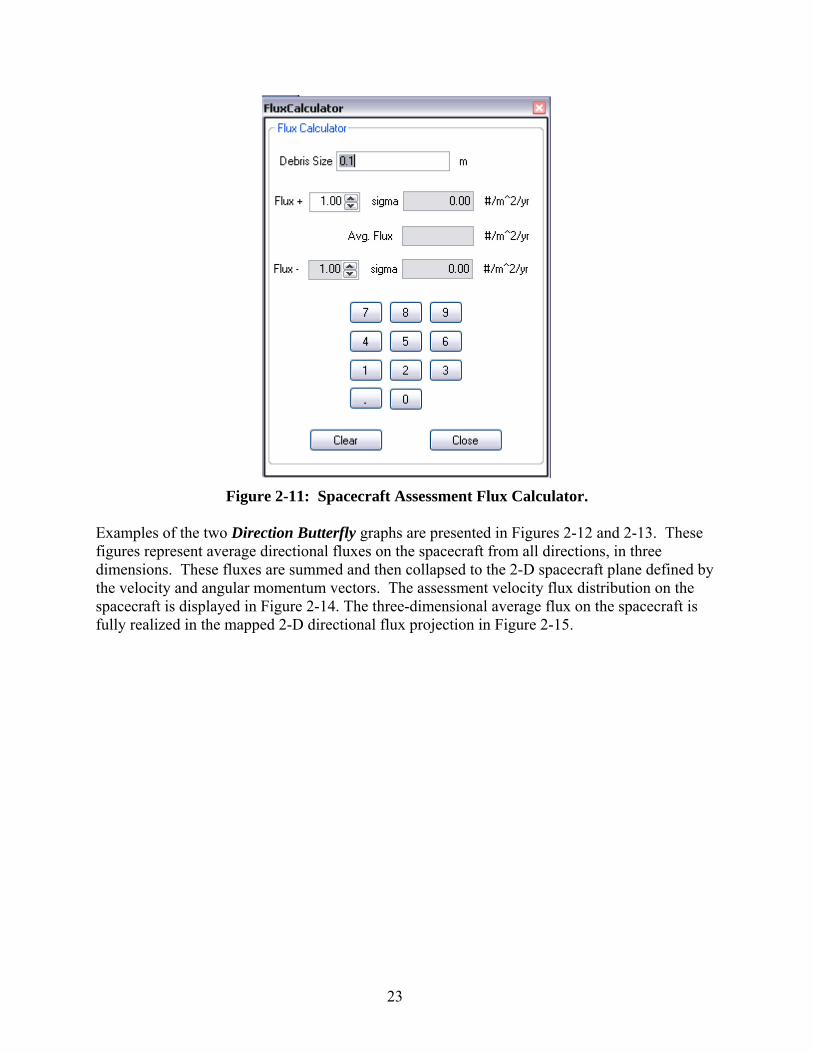
Figure 2-9: ORDEM 3.0 Spacecraft Assessment Graphs selection window. An example of the Average Flux vs. Size along the chosen spacecraft orbit is shown in Figure 2-10. It represents the particle flux at specific sizes and larger (i.e., cumulative flux) on a satellite over an orbit and has become a common metric of the debris environment for the ORDEM series, as well as for the ESA MASTER series. Given the proved utility of this type of chart and underlying data, a flux calculator is also included as an option associated with the Spacecraft assessment graphs. This function calculates flux given a particle size value and a chosen uncertainty of zero to three sigmas (Figure 2-11).

22

Figure 2-10: Spacecraft Assessment Average Flux vs. Size graph.

23

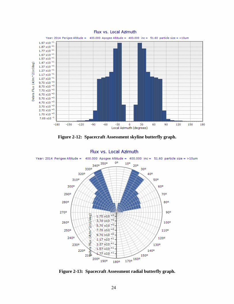
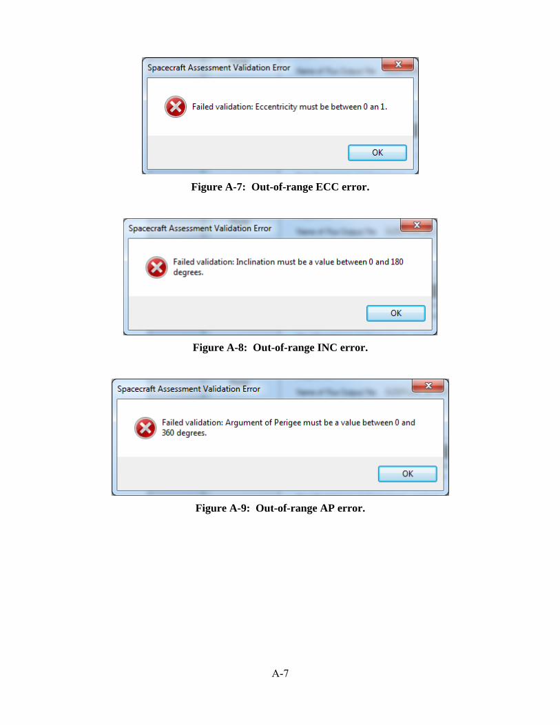
Figure 2-11: Spacecraft Assessment Flux Calculator. Examples of the two Direction Butterfly graphs are presented in Figures 2-12 and 2-13. These figures represent average directional fluxes on the spacecraft from all directions, in three dimensions. These fluxes are summed and then collapsed to the 2-D spacecraft plane defined by the velocity and angular momentum vectors. The assessment velocity flux distribution on the spacecraft is displayed in Figure 2-14. The three-dimensional average flux on the spacecraft is fully realized in the mapped 2-D directional flux projection in Figure 2-15.

24

Figure 2-12: Spacecraft Assessment skyline butterfly graph.

Figure 2-13: Spacecraft Assessment radial butterfly graph.

25

Figure 2-14: Spacecraft Assessment Velocity flux distribution.

Figure 2-15: Spacecraft Assessment 2-D Directional Flux projection. Direction relative to the spacecraft is noted in coordinates (local azimuth and local elevation): where azimuth runs along the horizontal from left to right and ranges from -180º to 180º and elevation

runs vertically from bottom to top and ranges from -90º to 90º.

26

2.4.2 Telescope/Radar Mode Graphs

After completing a computation, clicking the Graphs… button in the Telescope/Radar Assessment window initiates a new window, shown in Figure 2-16, from which a different graphical output is generated.

Figure 2-16: ORDEM 3.0 Telescope/Radar Assessment Graph selection window. Two examples of Flux vs. Altitude graphs are displayed in Figures 2-17 and 2-18 for the LEO and the GEO cases, respectively. These figures represent the surface area flux at specific sizes over altitude ranges in the Telescope/Radar mode.

Figure 2-17: Telescope/Radar Assessment Flux vs. Altitude graph, LEO region-only.

27

Figure 2-18: Telescope/Radar Assessment Flux vs. Altitude graph, GEO region-only. The flux curves below 10 cm in Figure 2-18 represent GTO objects at GEO altitudes (see Table 2-1). In an ORDEM 3.0 run (for both Spacecraft and Telescope/Radar modes), which calculates debris fluxes at altitudes higher than 2000 km, a status window warning message is displayed at the beginning and end of the run as in Figure 2-19.

28

Figure 2-19: Warning message in status window in both Spacecraft and Telescope/Radar modes for analysis apogees above 2000 km.

29

3.0 References

Kessler, D.J., 1984. Orbital Debris Environment for Space Station, JSC Internal Note 2001.

Kessler, D.J., et al., 1989. Orbital Debris Environment for Spacecraft Designed to Operate in Low Earth Orbit, NASA TM-100471.

Kessler, D.J., et al., 1991. Meteoroids and Orbital Debris, in Space Station Program Natural Environment Definition for Design, NASA SSP-30425/Rev. A.

Kessler, D.J., et al., 1996. A Computer-Based Orbital Debris Environment Model for Spacecraft Design and Observation in Low Earth Orbit, NASA TM-104825.

Liou, J.-C., et al., 2002. The New NASA Orbital Debris Engineering Model ORDEM2000. NASA/TP-2002-210780.

Oswald, M., et al., 2006. Upgrade of the MASTER Model, included in the MASTER-2005 package.

Sdunnus, H., et al., 2001. The ESA MASTER’99 Space Debris and Meteoroid Reference Model, Proceedings of the 3rd European Space Debris Conference, ESA SP-473.

A-1

Appendix A: ORDEM 3.0 Processor Messages and GUI Dialog Boxes

Table A.1 lists the message codes that may appear in the ORDEM 3.0 output text area. These codes are useful when diagnosing or reporting errors.

Table A.1. Processor Messages

Code Message ID Description

1 main_badasmtype Invalid assessment type in ‘ORDEM.IN’ file

2 main_badobsyr Observation year out of range in ‘ORDEM.IN’

3 main_badorbdeftype Orbit definition type out of range in ‘ORDEM.IN’

4 main_noini No input file 'ORDEM.IN'

5 main_badini Error reading ‘ORDEM.IN’ file

6 main_igorberr Fatal error in orbit mapping [igloo_orbit]

7 main_igpoperr Fatal error in population mapping [igloo_pop]

8 main_gensccalcserr Fatal error somewhere in sc_calcs

9 main_genscploterr Fatal error somewhere in generating the Spacecraft mode plot tables

10 main_badorbit Fatal error if the input orbit is nonsensical (i.e., perigee>apogee)

11 main_gentelecalcserr Fatal error somewhere in tele_calcs

12 main_gentelploterr Fatal error somewhere in generating the Telescope/Radar mode plot tables

13 main_numpopsmismatch Fatal error if population file read has a problem

14 main_noopsfile Fatal error if the operational errors file cannot be opened

15 main_datvermismatch Fatal error if the data versions mismatch (found in header of .POP files)

16 main_leohdryear Population file in the LEO data has incorrect year value

17 main_badleoigloobins Fatal error if the LEO igloo bins are nonsensical

18 main_badgeoigloobins Fatal error if the GEO igloo bins are nonsensical

19 main_leogeocntr Fatal error if the LEO/GEO counters are nonsensical

20 main_idbleo Fatal error if the idb totals of LEO data are not working

21 main_datamaprange Fatal error if the datamap range is out of range

22 main_popfileopen Cannot open the debris population data file

23 main_sobol Sobol General Error

24 main_sobol_read Cannot read Sobol coefficients data file

25 main_sobol_ unhandled Unhandled Sobol error

26 main_sobol_open Cannot open Sobol coefficients data file

27 main_geo_mm_open Cannot open GEO mean motion bin definitions file

28 main_geo_ecc_open Cannot open GEO eccentricity bin definitions file

29 main_geo_inc_open Cannot open GEO inclination bin definitions file

A-2


30 main_geo_raan_open Cannot open GEO RAAN bin definitions file

31 main_leo_hperi_open Cannot open LEO perigee alt. bin definitions file

32 main_leo_inc_open Cannot open LEO inclination bin definitions file

33 main_leo_ecc_open Cannot open LEO eccentricity bin definitions file

34 main_Runtimelog_open Cannot open the runtime log

35 main_geo_mm_read Error reading GEO mean motion bin definitions file

36 main_geo_ecc_read Error reading GEO eccentricity bin definitions file

37 main_geo_inc_read Error reading GEO inclination bin definitions file

38 main_geo_raan_read Error reading GEO RAAN bin definitions file

39 main_leo_hperi_read Error reading LEO perigee altitude bin definitions file

40 main_leo_inc_read Error reading LEO inclination bin definitions file

41 main_leo_ecc_read Error reading LEO eccentricity bin definitions file

42 main_populations_read Cannot read debris population data file

43 main_igloo_sc_open Cannot open Spacecraft igloo definition data file

44 main_igloo_sc_read Cannot read Spacecraft igloo definition data file

45 main_igloo_tel_open Cannot open Telescope/Radar igloo definition data file

46 main_igloo_tel_read Cannot read Telescope/Radar igloo definition data file

47 main_Runtimelog_read Error in test read of Runtimelog file

48 igorb_flux_sc_open Cannot open igloo flux file for output

49 igorb_sigran_sc_open Cannot open igloo flux random uncertainties file for output

50 igorb_sigpop_sc_open Cannot open igloo flux population uncertainties file for output

51 igorb_pop_sc_read Error reading debris population data file

52 igorb_sc_index Orbit index scheme violated

53 igorb_orbit_sc Incompatible selections in LEO (bad input configuration)

54 igorb_orbit_index Hperi, ecc, or inc bin index is out of range

55 igorb_numpops Number of populations input exceeded the number defined

56 igorb_lgcount Total population cells in GEO does not match computed

57 plotdata_sc_noflux Cannot open igloo flux (results) file

58 plotdata_sc_nosigpop Cannot open igloo flux population uncertainties file

59 plotdata_sc_nosigran Cannot open igloo flux random uncertainties file

60 plotdata_sc_sigran_read Cannot read igloo flux random uncertainties file

61 plotdata_sc_sigpop_read Cannot read igloo flux population uncertainties file

62 plotdata_sc_flux_read Cannot read igloo flux (results) file

63 sc_calcs_GEO_MM_read Cannot read GEO mean motion bin definition file

64 sc_calcs_sobol General Sobol failure

A-3


65 sc_calcs_sobol_read Cannot read Sobol coefficients data file

66 sc_calcs_GEO_ECC_read Cannot read GEO eccentricity bin definition file

67 sc_calcs_GEO_INC_read Cannot read GEO inclination bin definition file

68 sc_calcs_GEO_RAAN_read Cannot read GEO RAAN bin definition file

69 sc_calcs_IGLOO_SC_read Cannot read Spacecraft igloo bin definition file

70 sc_calcs_LEO_HPERI_read Cannot read LEO perigee altitude bin definition file

71 sc_calcs_LEO_ECC_read Cannot read LEO eccentricity bin definition file

72 sc_calcs_LEO_INC_read Cannot read LEO inclination bin definition file

73 sc_calcs_delta_az_small Igloo azimuth bin size is too small

74 sc_calcs_delta_az_big Igloo azimuth bin size is too large

75 sc_calcs_vel_min_small Igloo minimum velocity bin is too low

76 sc_calcs_vel_max_big Igloo maximum velocity bin is too high

77 sc_calcs_velmaxmin Igloo minimum velocity is higher than max. vel.

78 sc_calcs_delta_vel_small Igloo velocity bin size is too small

79 sc_calcs_delta_vel_big Igloo velocity bin size is too large

80 sc_calcs_delta_el_small Igloo elevation bin size is too small

81 sc_calcs_delta_el_big Igloo elevation bin size is too large

82 sc_calcs_IGLOO_NMAX Stated igloo dimensions do not match calculated dimensions

83 sc_calcs_IGLOO_CHECKICELL Failed igloocell check in Spacecraft mode

84 icell_open Failed match of igloocell

85 icell_mismatch Mismatch in population cell mapping

86 getinterp_cum Interpolation error

87 check_cum Cumulative Flux Check

88 sc_calcs_IGLOO_RANGELOCAL_AZ Azimuth bin is not bound

89 sc_calcs_IGLOO_AZ_RANGE Azimuth bin is out of bounds

90 sc_calcs_IGLOO_RANGELOCAL_EL Elevation bin is not bound

91 sc_calcs_IGLOO_EL_RANGE Elevation bin is out of bounds

92 sc_calcs_IGLOO_RANGELOCAL_VEL Velocity bin is not bound

93 sc_calcs_IGLOO_VEL_RANGE Velocity bin is out of bounds

94 sc_calcs_IGLOO_RANGE_WIDTH_AZ Azimuth bin has a bin size issue

95 sc_calcs_IGLOO_RANGE_WIDTH_EL Elevation bin has a bin size issue

96 sc_calcs_IGLOO_RANGE_WIDTH_VEL Velocity bin has a bin size issue

97 tele_calcs_sobol_read Sobol dimensioning is not correct

A-4


98 tele_calcs_GEO_MM_read Mean motion bin file is not able to be read

99 tele_calcs_GEO_ECC_read Eccentricity bin file is not able to be read

100 tele_calcs_GEO_INC_read Inclination bin file is not able to be read

101 tele_calcs_GEO_RAAN_read RAAN bin file is not able to be read

102 tele_calcs_LEO_HPERI_read Height perigee bin file is not able to be read

103 tele_calcs_LEO_ECC_read LEO Eccentricity file is not able to be read

104 tele_calcs_LEO_INC_read LEO Inclination file is not able to be read

105 tele_calcs_general Unknown error in the Telescope/Radar mode

106 main_path_proj Provided project path to ORDEM.exe is not valid

107 tele_leo_rng_minmax_calc Telescope/Radar min/max range problem

108 tele_leo_xe_lo Low radius debris orbit error

109 tele_leo_xe_hi High radius debris orbit error

110 plotdata_sc_sizeflux_open Cannot open SIZEFLUX_SC.OUT

111 plotdata_sc_velflux_open Cannot open VELFLUX_SC.OUT

112 plotdata_sc_dirflux_open Cannot open DIRFLUX_SC.OUT

113 plotdata_sc_butterfly_open Cannot open BFLY_SC.OUT

114 get_interp_cum_non_cumulative Cumulative interpolation error

115 match_cumu_3pt_bracketing 3‐point bracketing mismatch in cumulative interpolation

116 seek_igloocell_null_az Azimuth mismatch in igloo mapping function

117 seek_igloocell_null_el Elevation mismatch in igloo mapping function

118 seek_igloocell_null_vel Velocity mismatch in igloo mapping function

119 seek_igloocell_null_pole Pole mismatch in igloo mapping function

120 seek_igloocell_index_range Mapping function trying to go outside igloo range

121 seek_igloocell_az_limit Mapping function azimuth limit nonsensical

122 seek_igloocell_el_limit Mapping function elevation limit nonsensical

123 seek_igloocell_vel_limit Mapping function velocity limit nonsensical

124 bin_sequence_check_misalignment Bin sequence verification failed due to misalignment

125 bin_sequence_check_coherency Bin sequence verification failed due to incoherence

126 check_igflux_density Density bin is out of range

127 check_igflux_geo_density Density bin for GEO population is out of range

128 check_igflux_geo_cum GEO population is not loading in cumulative size

129 plotdata_sc_interpolation Interpolation error in Spacecraft mode sizeflux curve

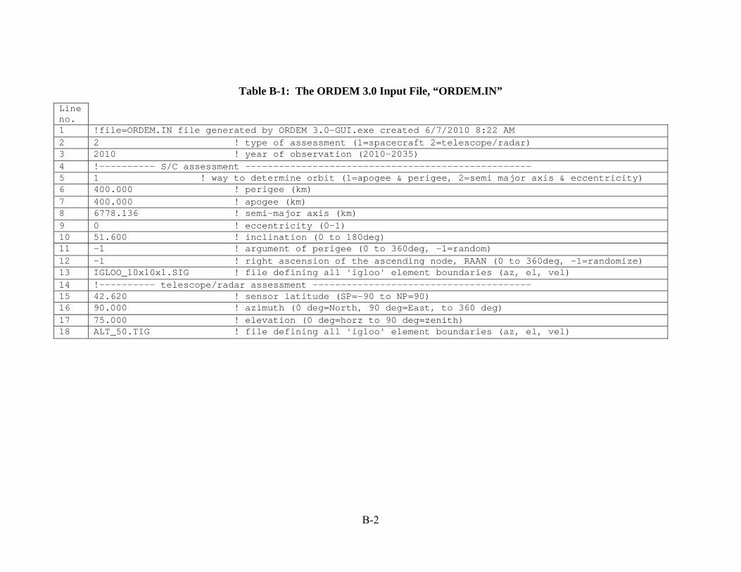
Figures A-1 through A-14 represent the possible GUI Dialog Boxes, which result when user inputs are invalid.

A-5

Figure A-1: Low perigee error.

Figure A-2: High perigee warning.

Figure A-3: Low apogee error.

A-6

Figure A-4: High apogee warning.

Figure A-5: Switched apogee and perigee error.

Figure A-6: Low semi-major axis error.

A-7

Figure A-7: Out-of-range ECC error.

Figure A-8: Out-of-range INC error.

Figure A-9: Out-of-range AP error.

A-8

Figure A-10: Out-of-range RAAN error.

Figure A-11: Out-of-range latitude error.

Figure A-12: Out-of-range azimuth error.

A-9

Figure A-13: Out-of-range elevation.

Figure A-14: Out-of-range flux calculator size.

B-1

Appendix B: ORDEM 3.0 Input/Output File Formats

This appendix contains sample file formats and descriptions of ORDEM 3.0 input and output files.

B.1 Input File Format

The ORDEM 3.0 input file containing all user-specified parameters is “ORDEM.IN”. This file is located in the project directory. The ORDEM 3.0 GUI creates this file as input for the computational run. When running ORDEM 3.0 using the command line interface, the user may create or edit the file using a simple text editor. (The user may wish to run the GUI once to create a template file.) The file contains both data and comments, the latter marked by the “!” character. ORDEM 3.0 reads specific values from specific lines of the file, so the format (as produced by the GUI) must be strictly followed. See Table B.1 for the file format and line-by-line descriptions. The first group of values (lines 2 through 3) specifies the type and year of assessment. The second group of values (lines 5 through 13) specifies the orbit and “Spacecraft encounter igloo” for Spacecraft assessment mode. The value on line 5 determines which two of the next four lines are used to define the input orbit, but the unused data lines must still be present to maintain the file format. The third group of values (lines 15 through 18) specifies the observer’s latitude and viewing angle, and “segmented bore-sight vector” to Telescope/Radar assessment mode.

B-2

Table B-1: The ORDEM 3.0 Input File, “ORDEM.IN”

Line no. 1 !file=ORDEM.IN file generated by ORDEM 3.0-GUI.exe created 6/7/2010 8:22 AM 2 2 ! type of assessment (1=spacecraft 2=telescope/radar) 3 2010 ! year of observation (2010-2035) 4 !---------- S/C assessment --------------------------------------------------- 5 1 ! way to determine orbit (1=apogee & perigee, 2=semi major axis & eccentricity) 6 400.000 ! perigee (km) 7 400.000 ! apogee (km) 8 6778.136 ! semi-major axis (km) 9 0 ! eccentricity (0-1) 10 51.600 ! inclination (0 to 180deg) 11 -1 ! argument of perigee (0 to 360deg, -1=random) 12 -1 ! right ascension of the ascending node, RAAN (0 to 360deg, -1=randomize) 13 IGLOO_10x10x1.SIG ! file defining all 'igloo' element boundaries (az, el, vel) 14 !---------- telescope/radar assessment --------------------------------------- 15 42.620 ! sensor latitude (SP=-90 to NP=90) 16 90.000 ! azimuth (0 deg=North, 90 deg=East, to 360 deg) 17 75.000 ! elevation (0 deg=horz to 90 deg=zenith) 18 ALT_50.TIG ! file defining all 'igloo' element boundaries (az, el, vel)

B-3

B.2 Output File Formats

This section has sample file formats of ORDEM 3.0 output. Table 2-9 is reprinted here as Table B-2 for reference. These text files may be used for external analysis but their main purpose is as interfaces between the program executable and the GUI.

Table B-2: Files Output by ORDEM 3.0 Modes


Spacecraft assessment output files

SIZEFLUX_SC.OUT Average impact cross-sectional area flux vs. size on the spacecraft along its orbit. Graph input.

VELFLUX_SC.OUT Impact velocity distribution on the spacecraft along its orbit. Graph input.

BFLY_SC.OUT Cross-sectional area flux vs. yaw (collapsed in pitch) in the spacecraft frame. Graph input.

DIRFLUX_SC.OUT Cross-sectional area flux in 2-D map projection in the spacecraft frame. Graph input.

IGLOOFLUX_SC.OUT Igloo element cross-sectional area fluxes and velocities. Intermediate file.

IGLOOFLUX_SIGMAPOP_SC.OUT Correlated population uncertainty estimates.

IGLOOFLUX_SIGMARAN_SC.OUT Random uncertainty estimates.

Telescope/Radar assessment output files

FLUX_TEL.OUT Surface area flux vs. altitude of debris of a given size. Graph input.

IGLOOFLUX_TEL.OUT Segmented bore-sight vector element fluxes. Intermediate file.

IGLOOFLUX_SIGMAPOP_TEL.OUT Correlated population uncertainty estimates.

IGLOOFLUX_SIGMARAN_TEL.OUT Random uncertainty estimates.

B.2.1 SIZEFLUX_SC.OUT

This is the output data for generating the plot of average, cumulative flux by particle size. It is the Spacecraft-mode graph “Average Flux vs. Size”. The file has five header lines (see Table B-3). The first column is the debris particle size threshold and the second column is the debris flux for debris of the stated size and larger. The third and fourth columns are the lower and upper one-sigma uncertainties, respectively.

B-4

Table B-3: Illustration of Output for SIZEFLUX_SC.OUT

ORDEM Spacecraft Mode Debris Flux (#/m^2/yr) Year: 2010 a = 6778.136 e = 0.000000 inc = 51.60 Size (m) Flux -Sigma +Sigma -------- -------- -------- -------- 1.00E-05 4.59E+02 3.35E+01 7.35E+01 1.02E-05 4.45E+02 7.17E+01 7.17E+01 1.05E-05 4.32E+02 7.00E+01 7.00E+01 . . . 9.55E-01 1.62E-07 1.43E-08 1.43E-08 9.77E-01 1.61E-07 1.42E-08 1.42E-08 1.00E+00 1.60E-07 1.42E-08 1.42E-08

B.2.2 VELFLUX_SC.OUT

This is the output file for generating the plot of debris flux as an impact relative velocity. It is the Spacecraft-mode graph “Velocity Distribution”. The file has eight header lines (as shown in Table B-4), including minimum and maximum values for each flux data column (useful for axis scaling). The first two columns define the lower and upper velocity bin bounds in km/s. Subsequent columns list the debris flux for each of several-size thresholds, as shown in the column headers.

Table B-4: Illustration of Output for VELFLUX_SC.OUT

ORDEM Spacecraft Mode Debris Flux (#/m^2/yr/kps) Year: 2010 a = 6778.136 e = 0.000000 inc = 51.63 Vel 1 Vel 2 >10um >100um >1mm >1cm >10cm >1m ----- ----- ----- ----- ----- ----- ----- -----Min.: 2.65E-01 3.13E-06 1.39E-06 3.29E-13 1.12E-11 8.56E-12Max.: 7.23E+01 3.23E+00 6.27E-03 4.61E-07 5.14E-08 2.41E-08----- ----- ----- ----- ----- ----- ----- ----- 0.0 0.1 9.17E-01 2.23E-02 1.92E-05 4.42E-09 2.51E-09 2.18E-09

0.1 0.2 9.17E-01 2.23E-02 1.92E-05 4.42E-09 2.51E-09 2.18E-090.2 0.3 9.17E-01 2.23E-02 1.92E-05 4.42E-09 2.51E-09 2.18E-09

.

.

. 22.7 22.8 1.00E-99 1.00E-99 1.00E-99 1.00E-99 1.00E-99 1.00E-99 22.8 22.9 1.00E-99 1.00E-99 1.00E-99 1.00E-99 1.00E-99 1.00E-99 22.9 23.0 1.00E-99 1.00E-99 1.00E-99 1.00E-99 1.00E-99 1.00E-99

B.2.3 BFLY_SC.OUT

This is the output file for generating the plot of debris flux as a local impact azimuth. It is the Spacecraft-mode graph “Direction Butterfly”. As defined in the Figure 2-12 caption, “local azimuth” is the angle, measured in the local horizontal plane, running

B-5

from left to right. The file has eight header lines (as shown in Table B-5), including minimum and maximum values for each flux data column (useful for axis scaling). The first two columns define the lower and upper azimuth bin bounds in degrees (positive to right of the velocity vector). Subsequent columns list the debris flux for each of several-size thresholds, as shown in the column headers.

Table B-5: Illustration of Output for BFLY_SC.OUT

ORDEM Spacecraft Mode Debris Flux (#/m^2/yr/deg)Year: 2010 a = 6778.136 e = 0.000000 inc = 51.63Az 1 Az 2 >10um >100um >1mm >1cm >10cm >1m----- ----- ----- ----- ----- ----- ----- -----Min.: 2.13E-02 3.77E-04 1.15E-06 7.08E-11 1.09E-11 1.85E-12Max.: 4.07E+00 1.82E-01 3.24E-04 2.32E-08 2.94E-09 1.49E-09----- ----- ----- ----- ----- ----- ----- ------180 -179 2.78E-02 1.33E-03 1.47E-05 8.07E-10 4.08E-11 2.03E-12-179 -178 2.78E-02 1.33E-03 1.47E-05 8.07E-10 4.08E-11 2.03E-12-178 -177 2.78E-02 1.33E-03 1.47E-05 8.07E-10 4.08E-11 2.03E-12. . . 177 178 2.78E-02 1.33E-03 1.47E-05 8.07E-10 4.08E-11 2.03E-12178 179 2.78E-02 1.33E-03 1.47E-05 8.07E-10 4.08E-11 2.03E-12179 180 2.78E-02 1.33E-03 1.47E-05 8.07E-10 4.08E-11 2.03E-12

B.2.4 DIRFLUX_SC.OUT

This is the output file for generating the plot of debris flux as a local impact azimuth and elevation. It is the Spacecraft-mode graph “2-D Directional Flux”, also known as a Mollweide projection. As defined in the Figure 2-15 caption, ”local azimuth” is the angle, measured in the local horizontal plane, running from left to right and “local elevation” is measured in a plane perpendicular to the local horizontal, running from bottom to top. The file has eight header lines (as shown in Table B-6), including minimum and maximum values for each flux data column (useful for axis scaling). The format of the output data was chosen for ease of use with the on-screen Mollweide plotting routine. The first eight columns define the corners of a box outline in X and Y coordinates. Consequently, “X_NE” and “Y_NE” are defined as the X and Y coordinates of the “northeast” corner of the box, as would be viewed on a flat map. With X and Y coordinates as Local Azimuth and Local Elevation, the pattern in the output file becomes clear. For example, minimum “X_NW” and “X_SW” is -180. Minimum “Y_SW” and “Y_SE” is -90. The box boundaries are easily identified in Figure 2-15 by color. The ninth and tenth columns list the central coordinate of the box outline, while subsequent columns list the debris flux for each of several-size thresholds, as shown in the column headers.

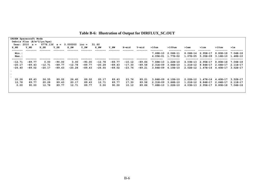
B-6

Table B-6: Illustration of Output for DIRFLUX_SC.OUT ORDEM Spacecraft Mode Debris Flux (#/m^2/yr/kps) Year: 2010 a = 6778.136 e = 0.000000 inc = 51.60 X_NE Y_NE X_SE Y_SE X_SW Y_SW X_NW Y_NW X-mid Y-mid >10um >100um >1mm >1cm >10cm >1m ------- ------- ------- ------- ------- ------- ------- ------- ------- ------- -------- -------- ------- -------- -------- -------- Min.: 7.68E-10 2.06E-11 8.06E-14 2.95E-17 8.80E-18 7.04E-18 Max.: 4.05E-01 1.77E-02 1.07E-05 5.35E-09 3.16E-10 1.48E-10 ------- ------- ------- ------- ------- ------- ------- ------- ------- ------- -------- -------- -------- -------- -------- -------- -12.71 -89.77 0.00 -90.00 0.00 -90.00 -12.78 -89.77 -10.12 -89.86 7.68E-10 1.22E-10 4.03E-13 2.95E-17 8.80E-18 7.04E-18 -20.17 -89.43 -12.71 -89.77 -12.78 -89.77 -20.28 -89.43 -17.30 -89.58 2.31E-09 3.66E-10 1.21E-12 8.84E-17 2.64E-17 2.11E-17 -26.40 -89.02 -20.17 -89.43 -20.28 -89.43 -26.55 -89.02 -23.76 -89.21 3.84E-09 6.10E-10 2.02E-12 1.47E-16 4.40E-17 3.52E-17 . . . 20.28 89.43 26.55 89.02 26.40 89.02 20.17 89.43 23.76 89.21 3.84E-09 6.10E-10 2.02E-12 1.47E-16 4.40E-17 3.52E-17 12.78 89.77 20.28 89.43 20.17 89.43 12.71 89.77 17.30 89.58 2.31E-09 3.66E-10 1.21E-12 8.84E-17 2.64E-17 2.11E-17 0.00 90.00 12.78 89.77 12.71 89.77 0.00 90.00 10.12 89.86 7.68E-10 1.22E-10 4.03E-13 2.95E-17 8.80E-18 7.04E-18

B-7

B.2.5 IGLOOFLUX_SC.OUT

The plottable files are derived from this output file. The file has five header lines (see Table B-7). The first column lists the encounter igloo element number. The second through seventh columns list the lower and upper azimuth bin bounds, lower and upper elevation bin bounds, and lower -and upper-relative-impact velocity bin bounds, respectively. Subsequent columns list the individual sub-population fluxes for the defined igloo element. The sub-population names are abbreviated using two letters for the population type and two numbers for the size (in powers of 10 µm). Debris type codes: NK - sodium-potassium (NaK) reactor coolant LD - general low-density debris ( <2 g/cc) MD - general medium-density debris (2-6 g/cc) HD - general high-density debris ( >6 g/cc) IN - intact/launched objects Debris size bin codes, in powers of 10 µm: “10” = 101.0 µm = 1.00e-5 m = 10 µm “15” = 101.5 µm = 3.16e-5 m = 31.6 µm “20” = 102.0 µm = 1.00e-4 m = 100 µm “25” = 102.5 µm = 3.16e-4 m = 316 µm “30” = 103.0 µm = 1.00e-3 m = 1 mm “35” = 103.5 µm = 3.16e-3 m = 3.16 mm “40” = 104.0 µm = 1.00e-2 m = 1 cm “45” = 104.5 µm = 3.16e-2 m = 3.16 cm “50” = 105.0 µm = 1.00e-1 m = 10 cm “55” = 105.5 µm = 3.16e-1 m = 31.6 cm “60” = 106.0 µm = 1.00e+0 m = 1 m

B-8

Table B-7: Illustration of Output for IGLOOFLUX_SC.OUT

ORDEM Debris flux through spacecraft 'igloo'.Igloo Debris Populations Flux in Bin (no./km^2/yr) Year: 2010 Elements: 14122 Populations: 55 a = 6778.136 e = 0.000000 inc = 51.60 Element az_low az_high el_low el_high vel_low vel_high Flux NK10 ... ------- -------- -------- -------- -------- -------- -------- ------------- 1 -180.00 180.00 -90.00 -85.00 0.00 1.00 0.0000000E+00 ...2 -180.00 180.00 -90.00 -85.00 1.00 2.00 0.0000000E+00 ...3 -180.00 180.00 -90.00 -85.00 2.00 3.00 0.0000000E+00 .... . . 14120 170.00 180.00 75.00 85.00 20.00 21.00 0.0000000E+00 ...14121 170.00 180.00 75.00 85.00 21.00 22.00 0.0000000E+00 ...14122 170.00 180.00 75.00 85.00 22.00 23.00 0.0000000E+00 ...

B-9

B.2.6 IGLOOFLUX_SIGMAPOP_SC.OUT

The format of this file is the same as that of IGLOOFLUX_SC.OUT, except the flux values are replaced by estimated population uncertainty values.

B.2.7 IGLOOFLUX_SIGMARAN_SC.OUT

The format of this file is the same as that of IGLOOFLUX_SC.OUT, except the flux values are replaced by estimated random uncertainty values.

B.2.8 FLUX_TEL.OUT

This is the output file for generating the plot of debris flux as an altitude or range within the beam. It is the Telescope/Radar-mode graph “Flux vs. Altitude”. The file has five header lines (see Table B-8). The first column lists the altitude bin boundaries for the data row. The second column lists the range, from the observer, corresponding to the altitude in the first column. Subsequent columns list the debris flux for each of several-size thresholds, as shown in the column headers.

Table B-8: Illustration of Output for FLUX_TEL.OUT

ORDEM Telescope/Radar Mode Surface Area Debris Flux (#/m^2/yr) Year: 2010 Sensor lat. = 42.620 Pointing AZ = 90.000 Pointing EL = 75.000 Alt Rng >10um >100um >1mm >1cm >10cm >1m ----- ----- ----- ----- ----- ----- ----- ----- 100.0 113.6 6.56E-01 1.25E-02 7.40E-04 2.89E-08 2.14E-09 9.53E-10150.0 165.2 6.56E-01 1.25E-02 7.40E-04 2.89E-08 2.14E-09 9.53E-10150.0 165.2 3.48E+00 4.00E-02 9.72E-04 4.09E-08 6.46E-09 4.07E-09. . . 39950.0 40147.5 9.50E-01 4.34E-02 8.72E-07 2.40E-11 6.71E-12 5.32E-1239950.0 40147.5 9.20E-01 4.21E-02 8.58E-07 2.35E-11 6.56E-12 5.20E-1240000.0 40197.5 9.20E-01 4.21E-02 8.58E-07 2.35E-11 6.56E-12 5.20E-12

B-10

B.2.9 IGLOOFLUX_TEL.OUT

The files with output that can be plotted are derived from this output file. The file has six header lines (see Table B-9). The first column lists the segmented bore-site vector element number. The second through fifth columns list the lower and upper altitude bin bounds, and lower and upper range bin bounds, respectively. Subsequent columns list the individual sub-population fluxes for the defined element. The sub-population names are identical to those defined in Section B.2.5.

B.2.10 IGLOOFLUX_SIGMAPOP_TEL.OUT

The format of this file is the same as that of IGLOOFLUX_TEL.OUT, except the flux values are replaced by estimated population uncertainty values.

B.2.11 IGLOOFLUX_SIGMARAN_TEL.OUT

The format of this file is the same as that of IGLOOFLUX_TEL.OUT, except the flux values are replaced by estimated random uncertainty values.

B-11

Table B-9: Illustration of Output for IGLOOFLUX_TEL.OUT

ORDEM Debris flux through telescope/radar 'igloo'. Igloo Debris Populations Flux in Bin (no./m^2/yr) Year: 2010 Elements: 798 Populations: 55 Sensor lat. = 46.620 Pointing AZ = 90.000 Pointing EL = 75.000 Element -------

alt_low ---------

alt high ---------

rng_low---------

rng high---------

Flux NK10 -------------

...

1 100.00 150.00 113.562 165.250 9.9130421E-08 ...2 150.00 200.00 165.250 216.911 4.0289432E-08 ...3 200.00 250.00 216.911 268.546 7.6370956E-08 ...

.

.

. 796 39850.00 39900.00 40047.392 40097.424 0.0000000E+00 ... 797 39900.00 39950.00 40097.424 40147.455 0.0000000E+00 ...798 39950.00 40000.00 40147.455 40197.487 0.0000000E+00 ...

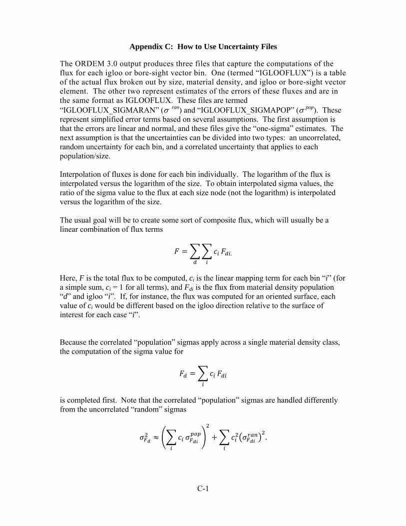
C-1

Appendix C: How to Use Uncertainty Files

The ORDEM 3.0 output produces three files that capture the computations of the flux for each igloo or bore-sight vector bin. One (termed “IGLOOFLUX”) is a table of the actual flux broken out by size, material density, and igloo or bore-sight vector element. The other two represent estimates of the errors of these fluxes and are in the same format as IGLOOFLUX. These files are termed “IGLOOFLUX_SIGMARAN” ( ran) and “IGLOOFLUX_SIGMAPOP” (pop). These represent simplified error terms based on several assumptions. The first assumption is that the errors are linear and normal, and these files give the “one-sigma” estimates. The next assumption is that the uncertainties can be divided into two types: an uncorrelated, random uncertainty for each bin, and a correlated uncertainty that applies to each population/size. Interpolation of fluxes is done for each bin individually. The logarithm of the flux is interpolated versus the logarithm of the size. To obtain interpolated sigma values, the ratio of the sigma value to the flux at each size node (not the logarithm) is interpolated versus the logarithm of the size. The usual goal will be to create some sort of composite flux, which will usually be a linear combination of flux terms

.

Here, F is the total flux to be computed, ci is the linear mapping term for each bin “i” (for a simple sum, ci = 1 for all terms), and Fdi is the flux from material density population “d” and igloo “i”. If, for instance, the flux was computed for an oriented surface, each value of ci would be different based on the igloo direction relative to the surface of interest for each case “i”. Because the correlated “population” sigmas apply across a single material density class, the computation of the sigma value for

is completed first. Note that the correlated “population” sigmas are handled differently from the uncorrelated “random” sigmas

.

C-2

The final total flux uncertainty is then assembled by

. Note this assumes that the uncertainties of each material density type are uncorrelated to those of other types. Note that to compute the expected value of impacts over some observation time on some oriented surface, the time and projected area values could be folded into the “ci” values for each flux case “i”. In this case the expected number of impacts N would be

.

where ci is now the projected area-time product of flux case “i” on the oriented surface of interest. The corresponding uncertainty propagation equations would be

D-1

Appendix D: ORDEM 3.0 Current Runtime Estimates

D.1 Runtime Estimates for Spacecraft Assessment Mode

The following estimates are based upon a large set of testing runs performed on a DELL Optiplex 760, with 2 GB of RAM and a limited amount of background tasks run concurrently with ORDEM 3.0. Actual runtimes may vary greatly depending on the object examined and computer capabilities. ORDEM 3.0 runtime estimates depend heavily on the user-chosen encounter igloo dimensions and the orbit being assessed. The binned population files are sparsely populated, but if an orbit located in a populated portion of that binned orbit space is chosen, there may be an exponential increase in calculations required to provide the user with flux and error bar estimates for the given orbit. In other cases, if the target satellite travels through spaces devoid of most debris, the runtime performance will increase markedly. For general runtime performance, it is useful to examine through what areas the target object travels. For LEO objects with nearly circular orbits (i.e., eccentricity 0.01) and an igloo of 10° x 10° x 1 km/s, runtime performance of the ORDEM 3.0 model should generally be between 10 and 30 minutes. As orbital eccentricity increases, the object travels through more of the orbital population space of the model, and runtime performance can exceed several hours. For some geosynchronous transfer orbit objects, it is possible for the model to take over 2 hours on a modestly equipped PC. These runtimes would generally decrease when the 30° x 30° x 2 km/s igloo is used.

D.2 Runtime Estimates for Telescope/Radar Assessment Mode

The runtime performance of the Telescope/Radar mode is just as dependent on the binned population space examined; however, in general, the runtimes are easier to predict. For a given latitude of the sensor, the runtime is dependent on the pointing direction (i.e., bore-sight vector). Runtime may change markedly because, for a random pointing direction at a random latitude, the sensor may be viewing portions of the population space that are highly or sparsely populated. For instance, if a Telescope/Radar is located at a latitude of 42.6 degrees and pointed due north, this sensor will view heavy debris populations in LEO-only. Populations above LEO will be very sparse. In a case where the sensor is pointing due south, debris with inclinations lower than 42.6° will be detected as well.

That being considered, the runtimes observed during testing, with a user-chosen, segmented bore-sight vector graduated in 50 km increments in altitude from LEO to GEO, were between 10 minutes and 2 hours. If the user desires a shorter runtime and if the application allows for it, the 50 km altitude gradation could be applied to LEO-only or GEO-only.

REPORT DOCUMENTATION PAGE Form Approved OMB No. 0704-0188

Public reporting burden for this collection of information is estimated to average 1 hour per response, including the time for reviewing instructions, searching existing data sources, gathering and

maintaining the data needed, and completing and reviewing the collection of information. Send comments regarding this burden estimate or any other aspect of this collection of information, including

suggestions for reducing this burden, to Washington Headquarters Services, Directorate for Information Operations and Reports, 1215 Jefferson Davis Highway, Suite 1204, Arlington, VA 22202-4302,

and to the Office of Management and Budget, Paperwork Reduction Project (0704-0188), Washington, DC 20503.

1. AGENCY USE ONLY (Leave Blank) 2. REPORT DATE 3. REPORT TYPE AND DATES COVERED

April 2014 NASA Technical Paper

4. TITLE AND SUBTITLE 5. FUNDING NUMBERS

NASA Orbital Debris Engineering Model ORDEM 3.0 - User’s Guide

6. AUTHOR(S)

Eugene G. Stansbery; Mark J. Matney; Paula H. Krisko; Phillip D. Anz-Meador; Matthew F.

Horstman; John N. Opiela; Eric Hillary; Nicole M. Hill; Robert L.Kelley

7. PERFORMING ORGANIZATION NAME(S) AND ADDRESS(ES) 8. PERFORMING ORGANIZATIONREPORT NUMBERS

Lyndon B. Johnson Space Center

Houston, Texas 77058

S-1132

9. SPONSORING/MONITORING AGENCY NAME(S) AND ADDRESS(ES) 10. SPONSORING/MONITORING

AGENCY REPORT NUMBER

National Aeronautics and Space Administration

Washington, DC 20546-0001

TP-2014-217370

11. SUPPLEMENTARY NOTES

12a. DISTRIBUTION/AVAILABILITY STATEMENT 12b. DISTRIBUTION CODE

Available from the NASA Center for AeroSpace Information (CASI) 7121 Standard Hanover, MD 21076-1320 Category: 61

13. ABSTRACT (Maximum 200 words)

The ORDEM 3.0 model is appropriate for engineering solutions requiring knowledge and estimates of the orbital debris environment.

It can also be used as a benchmark for ground-based debris measurements and observations. With significant improvements over its

predecessor, ORDEM 3.0 includes uncertainties in the flux estimates and material density classes. It has also been extended to

describe the orbital debris environment from low Earth orbit past geosynchronous orbit. A large set of observational data (both in-situ

and ground-based) reflect the current debris environment. Analytical techniques are employed to determine the orbit populations used

to calculate population fluxes and their uncertainties. The model output lists fluxes of debris in half-decade size bins by distinct

material characteristics (i.e., intact objects, high-, medium-, or low-material density objects, and NaK droplets) either by direction and

velocity for an encompassing ‘igloo’ (for spacecraft) or by range bins (for a sensor beam on the Earth’s surface), depending on the

user’s chosen operational mode. The program graphical user interface, executable data files, and an ORDEM 3.0 User’s Guide are

included. ORDEM 3.0 has been subjected to extensive verification and validation. Currently, ORDEM 3.0 runs on Windows XP or

more recent PC operating systems.

14. SUBJECT TERMS 15. NUMBER OF

PAGES

16. PRICE CODE

orbital debris; space debris; debris environment; debris flux; engineering model;

spacecraft safety; impact flux; OD Program Office; ORDEM 63

17. SECURITY CLASSIFICATION

OF REPORT


OF THIS PAGE


OF ABSTRACT

20. LIMITATION OF ABSTRACT

Unclassified Unclassified Unclassified Unlimited

Standard Form 298 (Rev Feb 89) (MS Word Mar 97) Prescribed by ANSI Std. 239-18 298-102

NSN 7540-01-280-5500

NASA Orbital Debris Engineering Model ORDEM 3.0 User’s Guide · NASA Orbital Debris Engineering...

Documents

Transcript of NASA Orbital Debris Engineering Model ORDEM 3.0 User’s Guide · NASA Orbital Debris Engineering...