
Nasa 1997 Symposium
346
DOT/FAA/AR-97/2, II Office of Aviation Research Washington, D.C. 20591 Proceedings of the FAA-NASA Symposium on the Continued Airworthiness of Aircraft Structures FAA Center of Excellence in Computational Modeling of Aircraft Structures Atlanta, Georgia August 28-30, 1997 July 1997 This document is available to the U.S. public through the National Technical Information Service, Springfield, Virginia 22161
-
Upload
airshowfan -
Category
Documents
-
view
97 -
download
3
Transcript of Nasa 1997 Symposium
DOT/FAA/AR-97/2, II
Office of Aviation ResearchWashington, D.C. 20591
Proceedings of theFAA-NASA Symposium on the ContinuedAirworthiness of Aircraft Structures
FAA Center of Excellence in Computational Modeling of Aircraft StructuresAtlanta, GeorgiaAugust 28-30, 1997
July 1997
This document is available to the U.S. publicthrough the National Technical InformationService, Springfield, Virginia 22161

NOTICE
This document is disseminated under the sponsorship of the U.S.Department of Transportation in the interest of information exchange. TheUnited States Government assumes no liability for the contents or usethereof. The United States Government does not endorse products ormanufacturers. Trade or manufacturer's names appear herein solelybecause they are considered essential to the objective of this report.
Technical Report Documentation Page
1. Report No.
DOT/FAA/AR-97/2, II
2. Government Accession No. 3. Recipient's Catalog No.
4. Title and Subtitle
PROCEEDINGS OF THEFAA-NASA SYMPOSIUM ON THE CONTINUED
5. Report Date
July 1997
AIRWORTHINESS OF AIRCRAFT STRUCTURES 6. Performing Organization Code
7. Author(s)
Compiled by Catherine A. Bigelow, Ph.D.
8. Performing Organization Report No.
9. Performing Organization Name and Address
Federal Aviation Administration NASA Langley Research CenterAirport and Aircraft Safety Materials Division
10. Work Unit No. (TRAIS)
Research and Development Division Hampton, VA 23681William J. Hughes Technical CenterAtlantic City International Airport, NJ 08405
11. Contract or Grant No.
12. Sponsoring Agency Name and Address
U.S. Department of TransportationFederal Aviation AdministrationOffice of Aviation Research
13. Type of Report and Period Covered
ProceedingsAugust 28-30, 1996
Washington, DC 20591 14. Sponsoring Agency Code
AAR-40015. Supplementary Notes
Edited by Catherine A. Bigelow, Ph.D, Federal Aviation Administration, William J. Hughes Technical Center
16. Abstract
This publication contains the fifty-two technical papers presented at the FAA-NASA Symposium on the ContinuedAirworthiness of Aircraft Structures. The symposium, hosted by the FAA Center of Excellence for Computational Modeling ofAircraft Structures at Georgia Institute of Technology, was held to disseminate information on recent developments inadvanced technologies to extend the life of high-time aircraft and design longer-life aircraft. Affiliations of the participantsincluded 33% from government agencies and laboratories, 19% from academia, and 48% from industry; in all 240 people werein attendance.
Technical papers were selected for presentation at the symposium, after a review of extended abstracts received by theOrganizing Committee from a general call for papers.
17. Key Words
Corrosion, Crack detection, Nondestructive inspection,Residual strength, Fatigue, Crack growth
18. Distribution Statement
Document is available to the public through the NationalTechnical Information Service, Springfield, Virginia 22161
19. Security Classif. (of this report)
Unclassified
20. Security Classif. (of this page)
Unclassified
21. No. of Pages
346
22. Price
Form DOT F1700.7 (8-72) Reproduction of completed page authorized
iii
CONTENTS
Volume I
Executive Summary ................................................................................................................vii
Airframe Life Extension Through Quantitative Rework Inspections, W. H. Sproat ................ 1
Analysis of a Composite Repair, C. Duong and J. Yu............................................................ 17
Analysis of Safety Performance Thresholds for Air Carriers by Using ControlCharting Techniques, A. Y. Cheng, J. T. Luxh• j, and R. Y. Liu...................................... 25
Analytical Approaches and Personal Computer (PC)-Based Design Package for BondedComposite Patch Repair, Y. Xiong, D. Raizenne, and D. Simpson.................................. 37
Analytical Fatigue Life Estimation of Full-Scale Fuselage Panel, J. Zhang,J. H. Park, and S. N. Atluri................................................................................................ 51
Analytical Methodology for Predicting the Onset of Widespread Fatigue Damagein Fuselage Structure, C. E. Harris, J. C. Newman, Jr., R. S. Piascik, and J. H.Starnes, Jr. ......................................................................................................................... 63
Application of Acoustic Emission to Health Monitoring of Helicopter MechanicalSystems, A. F. Almeida, W. D. Martin, and D. J. Pointer ................................................ 89
Applying United States Air Force Lessons Learned to Other Aircraft,G. D. Herring, R. D. Giese, and P. Toivonen.................................................................... 93
Automated Evaluation of Residual Strength in the Presence of Widespread FatigueDamage, W. T. Chow, H. Kawai, L. Wang, and S. N. Atluri ......................................... 101
Controlling Fatigue Failures by Means of a Trade-Off Between Design andInspection Parameters, A. Brot........................................................................................ 109
Controlling Human Error in Maintenance: Development and Research Activities,W. B. Johnson and W. T. Shepherd................................................................................ 117
Coordinated Metallographic, Chemical, and Electrochemical Analyses of FuselageLap Splice Corrosion, M. E. Inman, R. G. Kelly, S. A. Willard, and R. S. Piascik........ 129
Designing for the Durability of Bonded Structures, W. S. Johnson and L. M. Butkus......... 147
The Effect of Crack Interaction on Ductile Fracture, C. T. Sun and X. M. Su..................... 161
The Effect of Environmental Conditions and Load Frequency on the Crack InitiationLife and Crack Growth in Aluminum Structure, H.-J. Schmidt and B. Brandecker....... 171
iv
Effects of Combined Loads on the Nonlinear Response and Residual Strength ofDamaged Stiffened Shells, J. H. Starnes, Jr., C. A. Rose, and C. C. Rankin.................. 183
Elasto-Plastic Models for Interaction Between a Major Crack and Multiple SmallCracks, K. F. Nilsson ...................................................................................................... 197
An Energetic Characterization of the Propagation of Curved Cracks in Thin DuctilePlates, H. Okada and S. N. Atluri.................................................................................... 225
Engineering Fracture Parameters for Bulging Cracks in Pressurized UnstiffenedCurved Panels, J. G. Bakuckas, Jr., P. V. Nguyen, and C. A. Bigelow .......................... 239
Evaluation of Closure-Based Crack Growth Model, C. Hsu, K. K. Chan, and J. Yu........... 253
Failure Analysis of Aircraft Engine Containment Structures, S. Sarkar andS. N. Atluri ...................................................................................................................... 267
Fatigue and Damage Tolerance of Aging Aircraft Structures, G. I. Nesterenko................... 279
Fatigue Growth of Small Corner Cracks in Aluminum 6061-T651, R. L. Carlson,D. L. Steadman, D. S. Dancila, and G. A. Kardomateas................................................. 301
Fatigue Studies Related to Certification of Composite Crack Patching for PrimaryMetallic Aircraft Structure, A. Baker.............................................................................. 313
Volume II
Executive Summary ................................................................................................................vii
Fatigue-Life Prediction Methodology Using Small-Crack Theory and a Crack-ClosureModel, J. C. Newman, Jr., E. P. Phillips, and M. H. Swain............................................ 331
Full-Scale Glare Fuselage Panel Tests, R. W. A. Vercammen and H. H. Ottens................. 357
A Graphic User Interface (GUI) Front-End for Parametric Survey and its Applicationto Composite Patch Repairs of Metallic Structure, H. Kawai, H. Okada, andS. N. Atluri ...................................................................................................................... 369
Implementation and Application of a Large-Rotation Finite Element Formulation inNASA Code ZIP2DL, X. Deng and J. C. Newman, Jr.................................................... 377
Implications of Corrosion Pillowing on the Structural Integrity of FuselageLap Joints, N. C. Bellinger and J. P. Komorowski ......................................................... 391
Improved Nondestructive Inspection Techniques for Aircraft Inspection,D. Hagemaier and D. Wilson .......................................................................................... 403
v
Improving the Damage Tolerance of Bonded Structures Via Adhesive LayerBarriers, J. C. Brewer ...................................................................................................... 417
In Search of the Holy Grail—The Deterministic Prediction of Damage,D. D. Macdonald and J. Magalhaes................................................................................. 425
Investigation of Fuselage Structure Subject to Widespread Fatigue Damage,M. L. Gruber, K. E. Wilkins, and R. E. Worden............................................................. 439
Numerical Investigations into Viability of Crack Tip Opening Displacement as aFracture Parameter for Mixed-Mode I/II Tearing of Thin Aluminum Sheets,M. A. Sutton, W. Zhao, X. Deng, D. S. Dawicke, and J. C. Newman, Jr....................... 461
A Numerical Study of the Interactions Between Multiple Longitudinal Cracks in aFuselage (Multiple Discrete-Source Damages), W. T. Chow, L. Wang, H.Kawai, and S. N. Atluri ................................................................................................... 473
On-Aircraft Analysis of F-14 Aircraft Wing Bearings Using Acoustic EmissionTechniques, D. J. Pointer, W. D. Martin, and A. F. Almeida............................................. 481
Operator Concerns About Widespread Fatigue Damage and How it May BeHandled and Regulated in the Commercial Environment, D. V. Finch.......................... 487
Predictions of Stable Growth of a Lead Crack and Multiple-Site Damage Using Elastic-Plastic Finite Element Method (EPFEM) and Elastic-Plastic Finite ElementAlternating Method (EPFEAM), L. Wang, F. W. Brust, and S. N. Atluri ...................... 505
Predictions of Widespread Fatigue Damage Threshold, L. Wang, W. T. Chow, H.Kawai, and S. N. Atluri ................................................................................................... 519
Probability and Statistics Modeling of Constituent Particles and Corrosion Pits as aBasis for Multiple-Site Damage Analysis, N. R. Cawley, D. G. Harlow, andR. P. Wei ......................................................................................................................... 531
Probability-Based Cost-Effective Inspection Frequency for Aging TransportStructures, V. Li .............................................................................................................. 543
Residual Strength Predictions Using a Crack Tip Opening Angle Criterion,D. S. Dawicke.................................................................................................................. 555
A Review of Rotorcraft Structural Integrity/Airworthiness Approaches and Issues,D. P. Schrage................................................................................................................... 567
Rivet Bearing Load Considerations in the Design of Mechanical Repairs for AgingAircraft, H. Chickermane and H. C. Gea........................................................................ 577
vi
The Role of Fretting Crack Nucleation in the Onset of Widespread Fatigue Damage:Analysis and Experiments, M. P. Szolwinski, G. Harish, P. A. McVeigh, andT. N. Farris...................................................................................................................... 585
The Role of New-Technology Nondestructive Inspection (NDI) Techniques,A. Q. Howard .................................................................................................................. 597
Simulation of Stable Tearing and Residual Strength Prediction with Applications toAircraft Fuselages, C.-S. Chen, P. A. Wawrzynek, and A. R. Ingraffea......................... 605
A Study of Circumferential Cracks in the Presence of Multiple-Site Damage in anAircraft Fuselage, L. Wang, W. T. Chow, H. Kawai, J. Zhang, and S. N. Atluri ........... 619
A Study of Fatigue Crack Generation and Growth in Riveted Alcald 2024-T3Specimens, Z. M. Connor, M. E. Fine, and B. Moran .................................................... 631
T*ε Integrals for Curved Crack Growth, P. W. Lam, A. S. Kobayashi, H. Okada, S.N. Atluri, and P. W. Tan ................................................................................................. 643
Use of Neural Networks for Aviation Safety Risk Assessment, H.-J. Shyur,J. T. Luxhøj, and T. P. Williams..................................................................................... 655
Widespread Fatigue Damage Threshold Estimates, I. C. Whittaker and H. C. Chen........... 665
vii/viii
EXECUTIVE SUMMARY
The Federal Aviation Administration (FAA) and the National Aeronautics and SpaceAdministration (NASA) jointly sponsored the Symposium on Continued Airworthiness ofAircraft Structures in Atlanta, Georgia, August 28-30, 1996. The Symposium was hosted by theFAA Center of Excellence for Computational Modeling of Aircraft Structures at GeorgiaInstitute of Technology.
Technical papers were selected for presentation at the symposium, after a review of extendedabstracts received by the Organizing Committee from a general call for papers. Keynoteaddresses were given by Dr. George L. Donohue, Associate Administrator of Acquisition andResearch of the Federal Aviation Administration, and Dr. Robert W. Whitehead, AssociateAdministrator for Research and Acquisition, National Aeronautics and Space Administration.
Full-length manuscripts were requested from the authors of papers presented; these paper areincluded in the proceedings.
The members of the Conference Organizing Committee are as follows:
Chris C. Seher, Conference Chairman, Federal Aviation AdministrationCharles E. Harris, Conference Co-Chairman, NASA Langley Research CenterSatya N. Atluri, Georgia Institute of TechnologyAmos W. Hoggard, Douglas Aircraft CompanyRoy Wantanabe, Boeing Commercial Airplane GroupJohn W. Lincoln, US Air ForceThomas Swift, Federal Aviation AdministrationAubrey Carter, Delta AirlinesJerry Porter, Lockheed Martin AerospaceCatherine A. Bigelow, Federal Aviation AdministrationJames C. Newman, NASA Langley Research CenterAndres Zellweger, Federal Aviation Administration
Approximately 240 people attended the conference. The affiliations of the attendees included33% from government agencies and laboratories, 19% from academia, and 48% from industry.
Chris C. SeherFAA Technical Center
331
FATIGUE-LI FE PREDICTION METHODOLOGY USINGSMALL-CRACK THEORY AND A CRACK-CLOSURE MODEL
J. C. Newman, Jr. and E. P. PhillipsNASA Langley Research Center
Hampton, Virginia, USA
M. H. SwainLockheed Engineering and Sciences Company
Hampton, Virginia, USA
ABSTRACT
This paper reviews the capabilities of a plasticity-induced crack-closure model topredict fatigue lives of metallic materials using “small-crack theory” for various materialsand loading conditions. Crack tip constraint factors, to account for three-dimensional state-of-stress effects, were selected to correlate large-crack growth rate data as a function of the
effective-stress-intensity factor range (∆Keff) under constant-amplitude loading. Some
modifications to the ∆Keff -rate relations were needed in the near-threshold regime to fitmeasured small-crack growth rate behavior and fatigue endurance limits. The model wasthen used to calculate small- and large-crack growth rates and to predict total fatigue lives fornotched and unnotched specimens made of two aluminum alloys, a titanium alloy, and a steelunder constant-amplitude and spectrum loading. Fatigue lives were calculated using thecrack-growth relations and microstructural features like those that initiated cracks for thealuminum alloys and steel for edge-notched specimens. An equivalent-initial-flaw-sizeconcept was used to calculate fatigue lives in other cases. Results from the tests and analysesagreed well.
INTRODUCTION
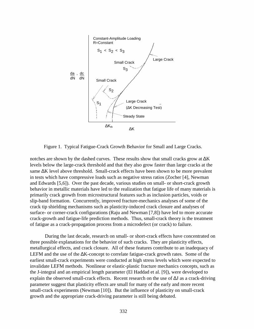
On the basis of linear-elastic fracture mechanics (LEFM), studies on small cracks (10µm to 1 mm) have shown that small cracks grow much faster than would be predicted fromlarge-crack data (Pearson [1], Ritchie and Lankford [2], Miller and de los Rios [3]). Thisbehavior is illustrated in Figure 1, where the crack-growth rate, da/dN or dc/dN, is plottedagainst the linear-elastic stress-intensity factor range, ∆Κ. The solid (sigmodal) curve showstypical results for large cracks in a given material and environment under constant-amplitudeloading. The solid curve is usually obtained from tests with large cracks. At low growth
rates, the threshold stress-intensity factor range, ∆Kth, is usually obtained from load-reduction (∆K-decreasing) tests. Some typical results for small cracks in plates and at
332
Figure 1. Typical Fatigue-Crack Growth Behavior for Small and Large Cracks.
notches are shown by the dashed curves. These results show that small cracks grow at ∆Klevels below the large-crack threshold and that they also grow faster than large cracks at thesame ∆K level above threshold. Small-crack effects have been shown to be more prevalentin tests which have compressive loads such as negative stress ratios (Zocher [4], Newmanand Edwards [5,6]). Over the past decade, various studies on small- or short-crack growthbehavior in metallic materials have led to the realization that fatigue life of many materials isprimarily crack growth from microstructural features such as inclusion particles, voids orslip-band formation. Concurrently, improved fracture-mechanics analyses of some of thecrack tip shielding mechanisms such as plasticity-induced crack closure and analyses ofsurface- or corner-crack configurations (Raju and Newman [7,8]) have led to more accuratecrack-growth and fatigue-life prediction methods. Thus, small-crack theory is the treatmentof fatigue as a crack-propagation process from a microdefect (or crack) to failure.
During the last decade, research on small- or short-crack effects have concentrated onthree possible explanations for the behavior of such cracks. They are plasticity effects,metallurgical effects, and crack closure. All of these features contribute to an inadequacy ofLEFM and the use of the ∆K-concept to correlate fatigue-crack growth rates. Some of theearliest small-crack experiments were conducted at high stress levels which were expected toinvalidate LEFM methods. Nonlinear or elastic-plastic fracture mechanics concepts, such asthe J-integral and an empirical length parameter (El Haddad et al. [9]), were developed toexplain the observed small-crack effects. Recent research on the use of ∆J as a crack-drivingparameter suggest that plasticity effects are small for many of the early and more recentsmall-crack experiments (Newman [10]). But the influence of plasticity on small-crackgrowth and the appropriate crack-driving parameter is still being debated.
Constant-amplitude loadingR = constant
Small crack
Small crack
Large crack
Large crack(DK decreasing test)
Steady state
DKth DK
da , dcdN dN__ __
S1
S2
S3
S1 < S2 < S3
Figure 1. Typical fatigue-crack growth behavior for small and large cracks
∆K
(∆K Decreasing Test)
Large Crack
Small Crack
Large CrackSmall Crack
∆Kth
Steady State
Constant-Amplitude LoadingR=Constant
333
Small cracks tend to initiate in metallic materials at inclusion particles or voids, inregions of intense slip, or at weak interfaces and grains. In these cases, metallurgicalsimilitude breaks down for these cracks (which means that the growth rate is no longer anaverage taken over many grains), see Leis et al. [11]. Thus, the local crack growth behavioris controlled by metallurgical features. If the material is markedly anisotropic, the local grainorientation will strongly influence the growth rate. Crack-front irregularities and smallparticles or inclusions affect the local stresses and, therefore, the crack growth response. Forlarge cracks, all of these metallurgical effects are averaged over many grains, except in verycoarse-grained materials. LEFM and nonlinear fracture mechanics concepts are onlybeginning to explore the influence of metallurgical features on stress-intensity factors, strain-energy densities, J-integrals, and other crack-driving parameters.
Very early in small-crack research, fatigue-crack closure (Elber [12]) was recognizedas a possible explanation for rapid small-crack growth rates (see Nisitani and Takao [13]).Fatigue-crack closure is caused by residual plastic deformations left in the wake of anadvancing crack. Only that portion of the load cycle for which the crack is fully open is used
in computing an effective stress-intensity factor range (∆Keff) from LEFM solutions. Asmall crack initiating at an inclusion particle, a void, or at a weak grain does not have theprior plastic history to develop closure. Thus, a small crack may not be closed for as muchof the loading cycle as a larger crack. If a small crack is fully open, the stress-intensity factorrange is fully effective and the crack-growth rate will be greater than steady-state, crack-growth rates. (A steady-state crack is one in which the residual plastic deformations andcrack closure along the crack surfaces are fully developed and stabilized under steady-stateloading.) Small-crack growth rates are also faster than steady-state behavior because thesecracks may initiate and grow in weak microstructure. In contrast to small-crack growthbehavior, the development of the large-crack threshold, as illustrated in Figure 1, has alsobeen associated with a rise in crack-opening load as the applied load is reduced (Minikawaand McEvily [14] and Newman [15]). Thus, the steady-state, crack-growth behavior may liebetween the small-crack and large-crack threshold behavior, as illustrated by the dash-dotcurve.
The purpose of this paper is to review the capabilities of a plasticity-induced, crack-closure model (Newman [16,17]) to correlate large-crack growth rate behavior and to predictfatigue lives in two aluminum alloys, a titanium alloy, and a steel under various loadhistories using small-crack theory. Test results from the literature on 2024-T3 and 7075-T6aluminum alloys, Ti-6Al-4V titanium alloy, and 4340 steel under constant-amplitude loadingwere analyzed with the closure model to establish an effective stress-intensity factor range
(∆Keff) against crack-growth rate relation. The ∆Keff -rate relation and some micro-structural features were used with the closure model to predict total fatigue lives on notchedspecimens made of aluminum alloys and steel under various load histories. An equivalent-initial-flaw-size (EIFS) concept (Rudd et al. [18]) was used to calculate fatigue lives forunnotched and notched aluminum and titanium alloys. The load histories considered wereconstant-amplitude loading over a wide range in stress ratios, FALSTAFF (van Dijk et al.[19]), Gaussian (Huck et al. [20]), TWIST (deJonge et al. [21]), Mini-TWIST (Lowak et al.[22]) and Felix/28 (Edwards and Darts [23]) load sequences. The crack configurations used
334
in these analyses were through-crack configurations, such as middle-crack and compacttension specimens, and three-dimensional crack configurations, such as a corner crack in abar or a surface crack at a circular hole or semicircular edge notch. Comparisons are madebetween measured and calculated or predicted fatigue lives on various unnotched andnotched specimens.
CRACK AND NOTCH CONFIGURATIONS ANALYZED
The large-crack, ∆K-rate data for the two aluminum alloys and the steel wereobtained from middle-crack tension specimens and the data for the titanium alloy wasobtained from compact tension and corner crack in a bar specimens. The data for the 2024-T3 alloy was obtained from Hudson [24], Phillips [25], and Dubensky [26], whereas the datafor the 7075-T6 alloy was obtained from Phillips and Deng (see Refs. 27 and 28). The datafor the 4340 steel was obtained from Swain et al. [29]. The data for the Ti-6Al-4V alloy wasobtained from Raizenne [30], Mom and Raizenne [31], and Powell and Henderson [32].
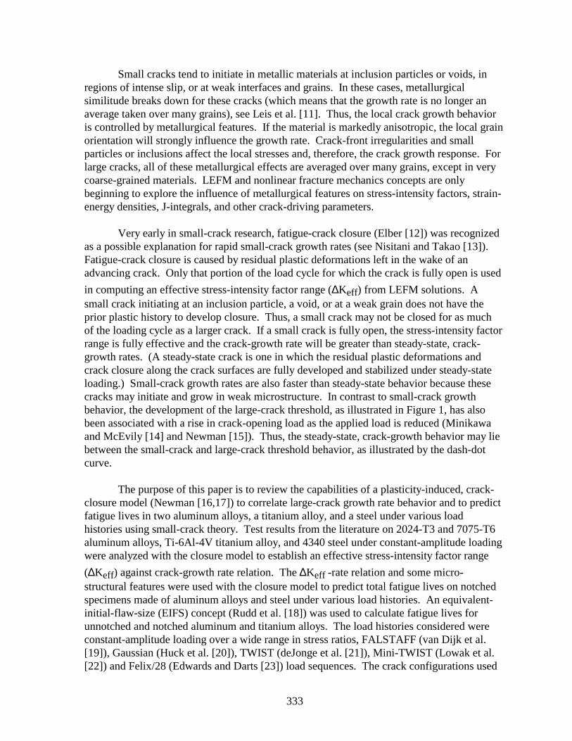
The fatigue specimens analyzed are shown in Figure 2. They were
(a) the uniform stress (KT = 1) unnotched specimen,(b) the circular-hole (KT = 3) specimen,(c) the single-edge-notch tension (SENT, KT = 3.15 or 3.3) specimen, and(d) the double-edge-notch tension (DENT, KT = 3.1) specimen.
Here the stress concentration factor, KT, is expressed in terms of the remote (gross) stress, S,instead of the net-section stress.
Figure 2. Fatigue Specimens Analyzed With Small-Crack Theory.
s s s s
(a) K = 1 (b) K = 3 (c) K = 3.15 (d) K = 3.1T T T T
w
w
2r
2w 2w
2r 2r
335
PLASTICITY-INDUCED CRACK-CLOSURE MODEL
The crack-closure model (Newman [16]) was developed for a central through crack ina finite-width specimen subjected to remote applied stress. The model was later extended toa through crack emanating from a circular hole and applied to the growth of small cracks(Newman [15]). The model was based on the Dugdale [33] model, but it was modified toleave plastically deformed material in the wake of the crack. The details of the model aregiven elsewhere and will not be presented here. One of the most important features of themodel, however, is the ability to model three-dimensional constraint effects. A constraint
factor, α, is used to elevate the flow stress (ασo) at the crack tip to account for the influence
of stress state. The flow stress σo is the average between the yield stress and ultimate tensilestrength. For plane-stress conditions, α is equal to unity (original Dugdale model), and forsimulated plane-strain conditions, α is equal to 3. Although the strip-yield model does notmodel the correct yield-zone pattern for plane-strain conditions, the model with a highconstraint factor is able to produce crack-surface displacements and crack-opening stressesquite similar to those calculated from an elastic-plastic finite element analysis of crackgrowth and closure for a finite-thickness plate (Blom et al. [34]). In conducting fatigue-crackgrowth analyses, the constraint factor α is used as a fitting parameter to correlate crack-
growth rate data against ∆Keff under constant-amplitude loading for different stress ratios.However, tests conducted under single-spike overloads seem to be more sensitive to state-of-stress effects and may be a more appropriate test to determine the constraint factor.
Effective Stress-Intensity Factor Range
For most damage tolerance and durability analyses, the linear-elastic analyses havebeen found to be adequate. The linear-elastic effective stress-intensity factor range developedby Elber [12] is given by
∆Keff = (Smax - S′o) √(πc) F(c/w) (1)
where Smax is the maximum stress, S′o is the crack-opening stress, and F is the boundary-correction factor. However, for high stress-intensity factors, proof testing, and low-cyclefatigue conditions, the linear-elastic analyses are inadequate and nonlinear crack-growthparameters are needed. To account for plasticity, a portion of the Dugdale cyclic-plastic-zonelength (ω) has been added to the crack length, c. The cyclic-plastic-zone corrected effectivestress-intensity factor [10] is
(∆Kp)eff = (Smax - S′o) √(πd) F(d/w) (2)
336
where d = c + ω/4 and F is the cyclic-plastic-zone corrected boundary-correction factor.Herein, the cyclic-plastic-zone corrected effective stress-intensity factor range will be used inthe fatigue-life predictions unless otherwise noted.
Constant-Amplitude Loading
As a crack grows in a finite-thickness body under cyclic loading (constant stressrange), the plastic-zone size at the crack front increases. At low stress-intensity factor levels,plane-strain conditions should prevail but as the plastic-zone size becomes large compared tosheet thickness, a loss of constraint is expected. This constraint loss has been associatedwith the transition from flat-to-slant crack growth. Schijve [35] has shown that the transitionoccurs at nearly the same crack-growth rate over a wide range in stress ratios for analuminum alloy. This observation has been used to help select the constraint-loss regime(see Ref. 36).
Newman [17] developed crack-opening stress equations for constant-amplitudeloading from crack-closure model calculations for a middle-crack tension specimen. Theseequations give crack opening stress as a function of stress ratio (R), maximum stress level
(Smax/σo), and the constraint factor (α). These equations are used to develop the baseline
∆Keff -rate relations that are used in the life-prediction code FASTRAN-II [37] to makecrack-growth and fatigue-life predictions.
LARGE-CRACK GROWTH BEHAVIOR
To make life predictions, ∆Keff as a function of the crack-growth rate must beobtained for the material of interest. Fatigue crack-growth rate data should be obtained overthe widest possible range in rates (from threshold to fracture), especially if spectrum loadpredictions are required. Data obtained on the crack configuration of interest would behelpful but it is not essential. The use of the nonlinear crack tip parameters is only necessaryif severe loading (such as low-cycle fatigue conditions) are of interest. Most damage-tolerantlife calculations can be performed using the linear elastic stress-intensity factor analysis withcrack-closure modifications.
Under constant-amplitude loading, the only unknown in the analysis is the constraintfactor, α. The constraint factor is determined by finding (by trial and error) an α value thatwill correlate the constant-amplitude fatigue crack-growth rate data over a wide range instress ratios, as shown by Newman [17]. This correlation should produce a unique
relationship between ∆Keff and crack-growth rate. In the large-crack-growth thresholdregime for some materials, the plasticity-induced closure model may not be able to collapse
337
the threshold (∆K-rate) data onto a unique ∆Keff -rate relation because of other forms ofclosure. Roughness- and oxide-induced closure (see Ritchie and Lankford [2]) appear to bemore relevant in the threshold regime than plasticity-induced closure. This may help explainwhy the constraint factors needed to correlate crack-growth rate data in the near thresholdregime are lower than plane-strain conditions. The constraint factors are 1.7 to 2 foraluminum alloys, 1.9 to 2.2 for titanium alloys, and 2.5 for steel. However, further study isneeded to assess the interactions between plasticity-, roughness- and oxide-induced closure
in this regime. If the plasticity-induced closure model is not able to give a unique ∆Keff -raterelation in the threshold regime, then high stress ratio (R ≥ 0.7) data may be used to establish
the ∆Keff -rate relation.
In the following, the ∆Keff -rate relation for two aluminum alloys, a titanium alloy,and a steel will be presented and discussed. A detailed description will be given for onematerial but similar procedures were used to establish the relationships for all materials usedin this study.
Aluminum Alloy 2024-T3
The large-crack results for 2024-T3 aluminum alloy are shown in Figure 3 for datagenerated by Hudson [24], Phillips [25], and Dubensky [26]. This figure shows the elastic
∆Keff (eqn. 1) plotted against crack-growth rate. The data collapsed into a narrow band withseveral transitions in slope occurring at about the same rate for all stress ratios. Some largedifferences were observed at high R-ratios in the high-rate regime. These tests wereconducted at extremely high remote stress levels (0.75 and 0.95 of the yield stress). Evenelastic-plastic analyses, such as equation 2, were unable to collapse the data along a uniquecurve in this regime. From a high-cycle fatigue standpoint, however, this discrepancy hasvery little influence on total life. The elastic-plastic fracture criterion (Two-Parameter
Fracture Criterion, TPFC; see Ref. 39) used in the analysis (KF = 267 MPa√m; m = 1)predicted failure very near to the vertical asymptotes of the test data, see the vertical dashedand dotted lines for R = 0.7 and 0.5 (at 0.75 and 0.95 of yield), respectively. Similar verticallines (not shown) would also indicate failure at the other R ratios. Lower R ratios would fail
at higher values of ∆Keff. For these calculations, a constraint factor (α) of 2.0 was used forrates less than 1E-07 m/cycle (start of transition from flat-to-slant crack growth) and α equalto 1.0 was used for rates greater than 2.5E-06 m/cycle (end of transition from flat-to-slantcrack growth). For intermediate rates, α was varied linearly with the logarithm of crack-growth rate (see Ref. 37). The values of α and rate were selected by trial and error and fromanalyses of crack growth under spectrum loading (see Ref. 38). The constraint-loss regime(α = 2 to 1) has also been associated with the flat-to-slant crack-growth behavior.
338
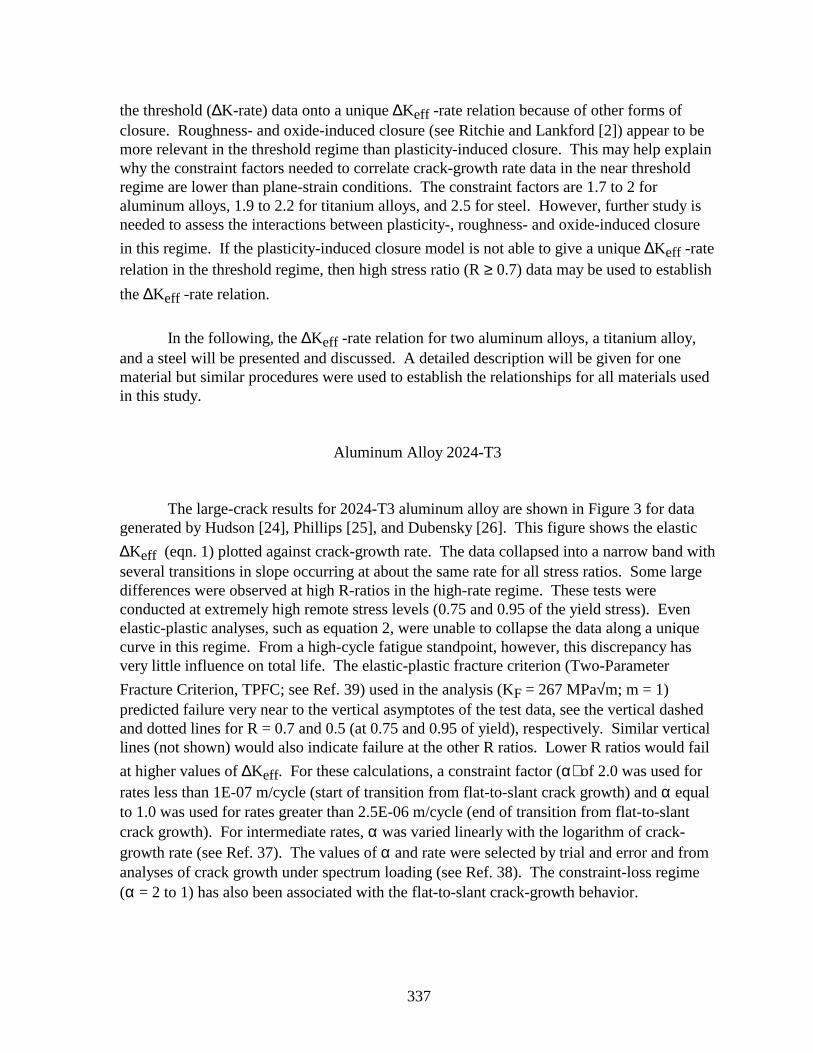
Reference 38 developed an expression to predict the location of the flat-to-slant crack-growthregime and the effective stress-intensity factor at transition is by
(∆Keff)T = 0.5 σo √B (3)
Figure 3. Effective Stress-Intensity Factor Range Against Crack-Growth Rate for LargeCracks in 2024-T3 Aluminum Alloy Sheet.
For the 2024-T3 alloy sheet, (∆Keff)T = 10.2 MPa√m. The width of the constraint-loss
regime, in terms of rate or ∆Keff, is a function of thickness but this relationship has yet to bedeveloped. In the low crack-growth rate regime, near and at threshold, tests and analyses[14,15] have indicated that the threshold develops because of a rise in the crack-openingstress-to-maximum-stress ratio due to the load-shedding procedure. In the threshold regime
then, the actual ∆Keff -rate data would lie at lower values of ∆Keff because the rise in crack-opening stress was not accounted for in the current analysis. For the present study, anestimate was made for this behavior on the basis of small-crack data [5] and it is shown bythe solid line below rates of about 2E-09 m/cycle. The baseline relation shown by the solidline (see Table 1) will be used later to predict fatigue lives under constant-amplitude andspectrum loading.
1 10 1001e-11
1e-10
1e-9
1e-8
1e-7
1e-6
1e-5
1e-4
1e-3
1e-2
DKeff, MPa-m1/2
dc/dNm/cycle
2024-T3 [24,25,26]Middle crack tensionB = 2.3 mm
a = 1
a = 2
R0.70.50.30-1-2
BaselineFailure (R = 0.7)Failure (R = 0.5)
∆ Keff, MPa-m1/2
2024-T3 [24, 25, 26]Middle Crack TensionB = 2.3 mm
2024-T3 [24, 25, 26]Middle-Crack TensionB = 2.3 mm
339
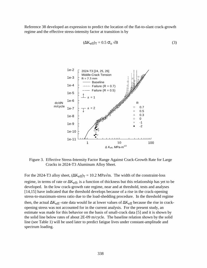
Table 1. Mechanical, Fracture, and Baseline Crack-Growth (∆Keff -Rate) Properties.
2024-T3 7075-T6 Ti-6Al-4V 4340 SteelB = 2.3 mm B = 2.3 mm B = 10-13 mm B = 5.1 mmσys = 360 MPa σys = 520 MPa σys = 860 MPa σys = 1410 MPaσu = 490 MPa σu = 575 MPa σu = 960 MPa σu = 1510 MPaE = 72000 MPa E = 72000 MPa E = 115000 MPa E = 207000 MPaKF = 267 MPa√m KF = 50 MPa√m KF = 54 MPa√m KF= 170 MPa√mm = 1.0 m = 0.0 m = 0.0 m = 0.0
∆Keff dc/dN ∆Keff dc/dN ∆Keff dc/dN ∆Keff dc/dNMPa√m m/cycle MPa√m m/cycle MPa√m m/cycle MPa√m m/cycle
0.8 1.0E-11 0.9 1.0E-11 1.0 1.0E-11 3.2 1.0E-111.05 1.0E-10 1.25 1.0E-09 2.5 1.0E-10 3.75 5.0E-102.05 2.0E-09 3.0 1.0E-08 4.4 1.0E-09 5.2 2.0E-094.0 8.0E-09 4.0 6.3E-08 8.0 1.0E-08 7.3 7.0E-097.7 1.0E-07 10.0 1.0E-06 12.8 1.0E-07 14.0 5.0E-0813.5 1.0E-06 14.8 1.0E-05 25.0 1.0E-06 50.0 6.5E-0723.0 1.0E-05 23.0 1.0E-04 54.0 2.0E-05 108.0 1.0E-0436.0 1.0E-0485.0 1.0E-02
α dc/dN α dc/dN α dc/dNm/cycle m/cycle m/cycle
2.0 1.0E-07 1.8 7.0E-07 α = 1.9 2.5 5.0E-071.0 2.5E-06 1.2 7.0E-06 1.2 2.5E-05
Aluminum Alloy 7075-T6
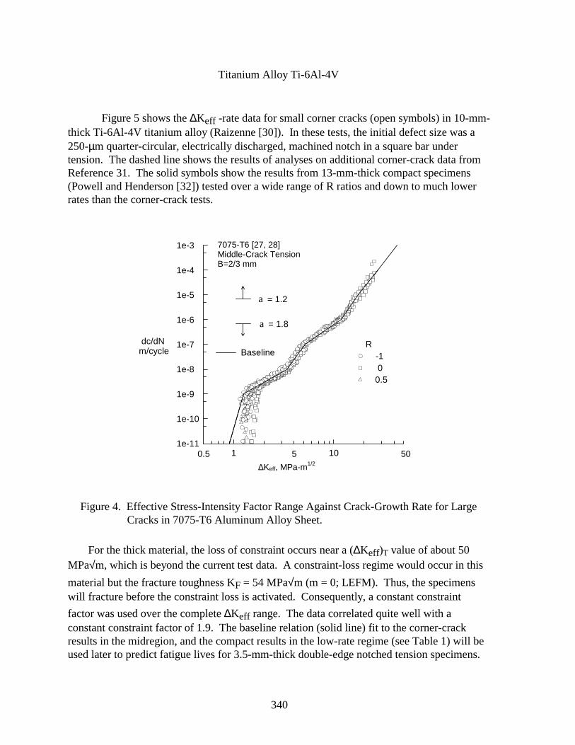
The large-crack results for 7075-T6 aluminum alloy are shown in Figure 4 for datagenerated at two different laboratories and at three stress ratios (Phillips and Deng, seeRef. 27). The data collapsed into a narrow band, again, with several transitions in slopeoccurring at about the same rate for all stress ratios. These data demonstrate why a table-
lookup ∆Keff-rate curve is needed to fit crack-growth rate data over many orders ofmagnitude in rate. Some differences were observed in the near threshold regime. For thesecalculations, a constraint factor α of 1.8 was used for rates less than 7E-07 m/cycle and αequal to 1.2 for rates greater than 7E-06 m/cycle. Again, the values of α and rate wereselected by trial and error. For this sheet alloy, the constraint-loss regime occurs near
(∆Keff)T = 13.1 MPa√m. In the threshold regime, an estimate was made to fit small-crackgrowth rate behavior (see Ref. 28) and it is shown by the solid line below a rate of about 2E-09 m/cycle. The baseline relation shown by the solid line (see Table 1) will be used later topredict small-crack growth rates and fatigue lives under constant-amplitude and spectrumloading.
340
Titanium Alloy Ti-6Al-4V
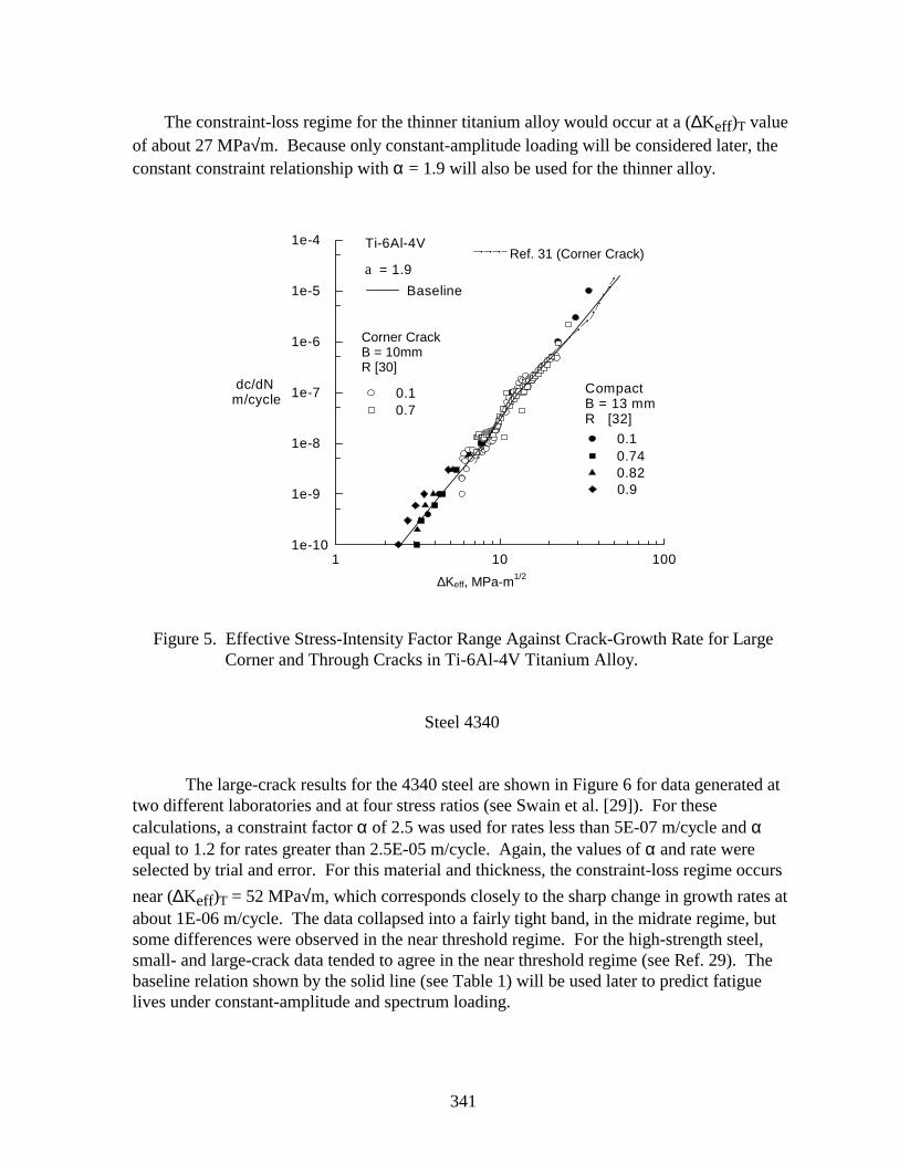
Figure 5 shows the ∆Keff -rate data for small corner cracks (open symbols) in 10-mm-thick Ti-6Al-4V titanium alloy (Raizenne [30]). In these tests, the initial defect size was a250-µm quarter-circular, electrically discharged, machined notch in a square bar undertension. The dashed line shows the results of analyses on additional corner-crack data fromReference 31. The solid symbols show the results from 13-mm-thick compact specimens(Powell and Henderson [32]) tested over a wide range of R ratios and down to much lowerrates than the corner-crack tests.
1 101e-11
1e-10
1e-9
1e-8
1e-7
1e-6
1e-5
1e-4
1e-3
DKeff, MPa-m1/2
dc/dN m/cycle
0.5 5 50
7075-T6 [27,28]Middle crack tensionB = 2.3 mm
a = 1.2
a = 1.8
BaselineR
-1 00.5
Figure 4. Effective Stress-Intensity Factor Range Against Crack-Growth Rate for LargeCracks in 7075-T6 Aluminum Alloy Sheet.
For the thick material, the loss of constraint occurs near a (∆Keff)T value of about 50MPa√m, which is beyond the current test data. A constraint-loss regime would occur in this
material but the fracture toughness KF = 54 MPa√m (m = 0; LEFM). Thus, the specimenswill fracture before the constraint loss is activated. Consequently, a constant constraint
factor was used over the complete ∆Keff range. The data correlated quite well with aconstant constraint factor of 1.9. The baseline relation (solid line) fit to the corner-crackresults in the midregion, and the compact results in the low-rate regime (see Table 1) will beused later to predict fatigue lives for 3.5-mm-thick double-edge notched tension specimens.
7075-T6 [27, 28]Middle-Crack TensionB=2/3 mm
∆Keff, MPa-m1/2
341
The constraint-loss regime for the thinner titanium alloy would occur at a (∆Keff)T valueof about 27 MPa√m. Because only constant-amplitude loading will be considered later, theconstant constraint relationship with α = 1.9 will also be used for the thinner alloy.
1 10 1001e-10
1e-9
1e-8
1e-7
1e-6
1e-5
1e-4
DKeff, MPa-m1/2
dc/dNm/cycle
Ti-6Al-4V
a = 1.9
Baseline
Corner crackB = 10 mmR [30]
CompactB = 13 mmR [32]
0.10.7
0.10.740.820.9
Ref 31 (Corner crack)
Figure 5. Effective Stress-Intensity Factor Range Against Crack-Growth Rate for LargeCorner and Through Cracks in Ti-6Al-4V Titanium Alloy.
Steel 4340
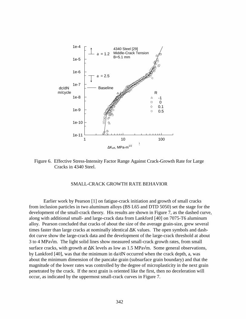
The large-crack results for the 4340 steel are shown in Figure 6 for data generated attwo different laboratories and at four stress ratios (see Swain et al. [29]). For thesecalculations, a constraint factor α of 2.5 was used for rates less than 5E-07 m/cycle and αequal to 1.2 for rates greater than 2.5E-05 m/cycle. Again, the values of α and rate wereselected by trial and error. For this material and thickness, the constraint-loss regime occurs
near (∆Keff)T = 52 MPa√m, which corresponds closely to the sharp change in growth rates atabout 1E-06 m/cycle. The data collapsed into a fairly tight band, in the midrate regime, butsome differences were observed in the near threshold regime. For the high-strength steel,small- and large-crack data tended to agree in the near threshold regime (see Ref. 29). Thebaseline relation shown by the solid line (see Table 1) will be used later to predict fatiguelives under constant-amplitude and spectrum loading.
∆Keff, MPa-m1/2
Ref. 31 (Corner Crack)
Corner CrackB = 10mmR [30]
342
1 10 1001e-11
1e-10
1e-9
1e-8
1e-7
1e-6
1e-5
1e-4
DKeff, MPa-m1/2
4340 Steel [29]Middle crack tensionB = 5.1 mm
R-1 00.10.5
dc/dNm/cycle
a = 2.5
a = 1.2
Baseline
Figure 6. Effective Stress-Intensity Factor Range Against Crack-Growth Rate for LargeCracks in 4340 Steel.
SMALL-CRACK GROWTH RATE BEHAVIOR
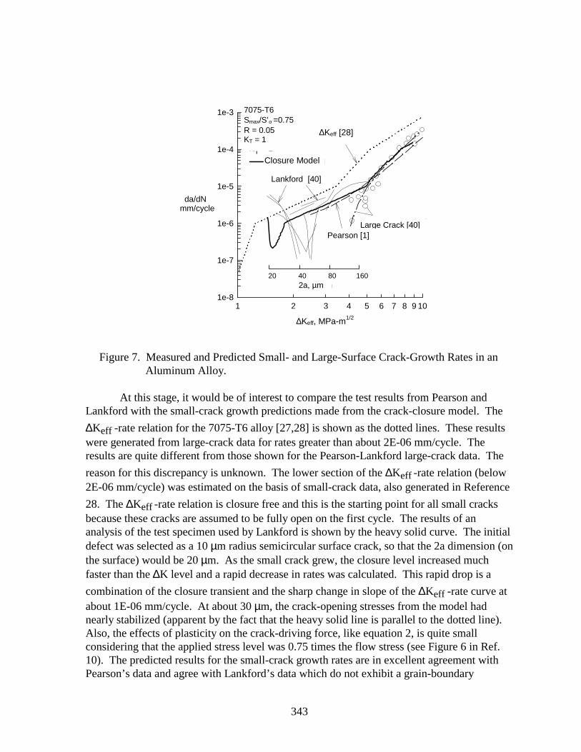
Earlier work by Pearson [1] on fatigue-crack initiation and growth of small cracksfrom inclusion particles in two aluminum alloys (BS L65 and DTD 5050) set the stage for thedevelopment of the small-crack theory. His results are shown in Figure 7, as the dashed curve,along with additional small- and large-crack data from Lankford [40] on 7075-T6 aluminumalloy. Pearson concluded that cracks of about the size of the average grain-size, grew severaltimes faster than large cracks at nominally identical ∆K values. The open symbols and dash-dot curve show the large-crack data and the development of the large-crack threshold at about3 to 4 MPa√m. The light solid lines show measured small-crack growth rates, from smallsurface cracks, with growth at ∆K levels as low as 1.5 MPa√m. Some general observations,by Lankford [40], was that the minimum in da/dN occurred when the crack depth, a, wasabout the minimum dimension of the pancake grain (subsurface grain boundary) and that themagnitude of the lower rates was controlled by the degree of microplasticity in the next grainpenetrated by the crack. If the next grain is oriented like the first, then no deceleration willoccur, as indicated by the uppermost small-crack curves in Figure 7.
∆Keff, MPa-m1/2
4340 Steel [29]Middle-Crack TensionB=5.1 mm
343
DK, MPa-m1/2
2 3 4 5 6 7 8 91 10
da/dNmm/cycle
1e-8
1e-7
1e-6
1e-5
1e-4
1e-3 7075-T6 Smax/so = 0.75R = 0.05KT = 1
20 40 80 1602a, mm
Large crack [40]
Pearson [1]
DKeff [28]
Closure model
Lankford [40]
Figure 7. Measured and Predicted Small- and Large-Surface Crack-Growth Rates in anAluminum Alloy.
At this stage, it would be of interest to compare the test results from Pearson andLankford with the small-crack growth predictions made from the crack-closure model. The
∆Keff -rate relation for the 7075-T6 alloy [27,28] is shown as the dotted lines. These resultswere generated from large-crack data for rates greater than about 2E-06 mm/cycle. Theresults are quite different from those shown for the Pearson-Lankford large-crack data. The
reason for this discrepancy is unknown. The lower section of the ∆Keff -rate relation (below2E-06 mm/cycle) was estimated on the basis of small-crack data, also generated in Reference
28. The ∆Keff -rate relation is closure free and this is the starting point for all small cracksbecause these cracks are assumed to be fully open on the first cycle. The results of ananalysis of the test specimen used by Lankford is shown by the heavy solid curve. The initialdefect was selected as a 10 µm radius semicircular surface crack, so that the 2a dimension (onthe surface) would be 20 µm. As the small crack grew, the closure level increased muchfaster than the ∆K level and a rapid decrease in rates was calculated. This rapid drop is a
combination of the closure transient and the sharp change in slope of the ∆Keff -rate curve atabout 1E-06 mm/cycle. At about 30 µm, the crack-opening stresses from the model hadnearly stabilized (apparent by the fact that the heavy solid line is parallel to the dotted line).Also, the effects of plasticity on the crack-driving force, like equation 2, is quite smallconsidering that the applied stress level was 0.75 times the flow stress (see Figure 6 in Ref.10). The predicted results for the small-crack growth rates are in excellent agreement withPearson’s data and agree with Lankford’s data which do not exhibit a grain-boundary
∆Keff, MPa-m1/2
Closure Model
Large Crack [40]
∆Keff [28]
7075-T6Smax/S′o =0.75R = 0.05KT = 1
2a, µm
344
influence. Interestingly, the small-crack analysis shows a single dip in the small-crack curve,similar to the single dip observed in some of Lankford’s small-crack data. Would the grain-boundary interaction always occur at the same crack length (40 µm)? Why aren’t there otherdips, or small indications of a dip, in the rate curve at 80, 120, or 160 µm? Further study isneeded to help resolve these issues. The following section will review the use of small-cracktheory to predict or calculate fatigue life for unnotched and notched specimens under variousload histories.
FATIGUE-LIFE PREDICTIONS
At this point, all of the elements are in place to assess small-crack theorya totalfatigue-life prediction methodology based solely on crack propagation from microstructuralfeatures. In this approach, a crack is assumed to initiate and grow from a microstructuralfeature on the first cycle. The crack-closure model and the baseline ∆Keff -rate curve are usedto predict crack growth from the initial crack size to failure. The final crack size wascalculated from the fracture toughness of the material, except where noted. Comparisons aremade with fatigue tests conducted on unnotched tension, circular-hole tension, and single- ordouble-edge notch tension specimens. Results are presented for two aluminum alloys, atitanium alloy, and a high-strength steel under either constant-amplitude or spectrum loading.
Aluminum Alloy 2024-T3
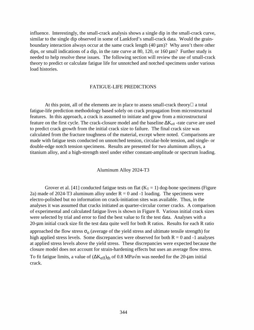
Grover et al. [41] conducted fatigue tests on flat (KT = 1) dog-bone specimens (Figure2a) made of 2024-T3 aluminum alloy under R = 0 and -1 loading. The specimens wereelectro-polished but no information on crack-initiation sites was available. Thus, in theanalyses it was assumed that cracks initiated as quarter-circular corner cracks. A comparisonof experimental and calculated fatigue lives is shown in Figure 8. Various initial crack sizeswere selected by trial and error to find the best value to fit the test data. Analyses with a20-µm initial crack size fit the test data quite well for both R ratios. Results for each R ratio
approached the flow stress σo (average of the yield stress and ultimate tensile strength) forhigh applied stress levels. Some discrepancies were observed for both R = 0 and -1 analysesat applied stress levels above the yield stress. These discrepancies were expected because theclosure model does not account for strain-hardening effects but uses an average flow stress.
To fit fatigue limits, a value of (∆Keff)th of 0.8 MPa√m was needed for the 20-µm initialcrack.
345
Nf, cycles
1e+2 1e+3 1e+4 1e+5 1e+6 1e+7 1e+8
Smax MPa
0
100
200
300
400
500
sys
su
2024-T3 [41]B = 2.3 mmw = 25.4 mmKT = 1
R = -1
R = 0
Closure modelai = ci = 20 mm
Figure 8. Measured and Calculated Fatigue Lives for 2024-T3 Aluminum Alloy UnnotchedSpecimens.
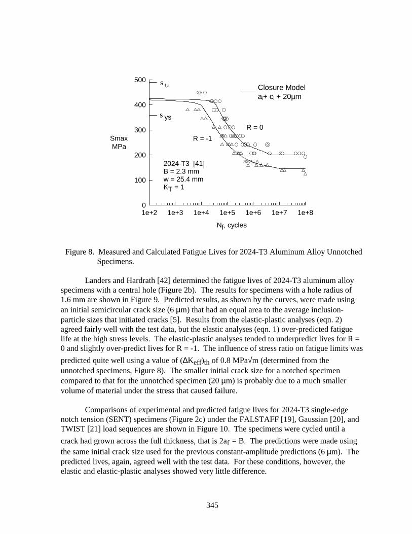
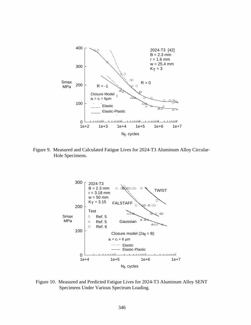
Landers and Hardrath [42] determined the fatigue lives of 2024-T3 aluminum alloyspecimens with a central hole (Figure 2b). The results for specimens with a hole radius of1.6 mm are shown in Figure 9. Predicted results, as shown by the curves, were made usingan initial semicircular crack size (6 µm) that had an equal area to the average inclusion-particle sizes that initiated cracks [5]. Results from the elastic-plastic analyses (eqn. 2)agreed fairly well with the test data, but the elastic analyses (eqn. 1) over-predicted fatiguelife at the high stress levels. The elastic-plastic analyses tended to underpredict lives for R =0 and slightly over-predict lives for R = -1. The influence of stress ratio on fatigue limits was
predicted quite well using a value of (∆Keff)th of 0.8 MPa√m (determined from theunnotched specimens, Figure 8). The smaller initial crack size for a notched specimencompared to that for the unnotched specimen (20 µm) is probably due to a much smallervolume of material under the stress that caused failure.
Comparisons of experimental and predicted fatigue lives for 2024-T3 single-edgenotch tension (SENT) specimens (Figure 2c) under the FALSTAFF [19], Gaussian [20], andTWIST [21] load sequences are shown in Figure 10. The specimens were cycled until a
crack had grown across the full thickness, that is 2af = B. The predictions were made usingthe same initial crack size used for the previous constant-amplitude predictions (6 µm). Thepredicted lives, again, agreed well with the test data. For these conditions, however, theelastic and elastic-plastic analyses showed very little difference.
Closure Modelai+ ci + 20µm
346
Nf, cycles
1e+2 1e+3 1e+4 1e+5 1e+6 1e+7
Smax MPa
0
100
200
300
400 2024-T3 [42]B = 2.3 mmr = 1.6 mmw = 25.4 mmKT = 3
R = 0R = -1
Closure modelai = ci = 6 mm
ElasticElastic-plastic
Figure 9. Measured and Calculated Fatigue Lives for 2024-T3 Aluminum Alloy Circular-Hole Specimens.
Nf, cycles
1e+4 1e+5 1e+6 1e+7
Smax MPa
0
100
200
300 2024-T3B = 2.3 mmr = 3.18 mmw = 50 mmKT = 3.15
TWIST
FALSTAFF
Gaussian
TestRef. 5Ref. 5Ref. 6
Closure model (2af = B)ai = ci = 6 mm
ElasticElastic-plastic
Figure 10. Measured and Predicted Fatigue Lives for 2024-T3 Aluminum Alloy SENTSpecimens Under Various Spectrum Loading.
Closure Modelai = ci = 6µm
Elastic
Elastic-Plastic
ElasticElastic-Plastic
ai = ci = 6 µm
347
Aluminum Alloy 7075-T6
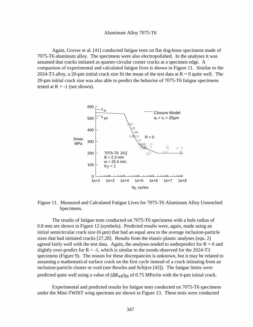
Again, Grover et al. [41] conducted fatigue tests on flat dog-bone specimens made of7075-T6 aluminum alloy. The specimens were also electropolished. In the analyses it wasassumed that cracks initiated as quarter-circular corner cracks at a specimen edge. Acomparison of experimental and calculated fatigue lives is shown in Figure 11. Similar to the2024-T3 alloy, a 20-µm initial crack size fit the mean of the test data at R = 0 quite well. The20-µm initial crack size was also able to predict the behavior of 7075-T6 fatigue specimenstested at R = -1 (not shown).
Nf, cycles
1e+2 1e+3 1e+4 1e+5 1e+6 1e+7 1e+8
Smax MPa
0
100
200
300
400
500
600
sys
su
7075-T6 [41]B = 2.3 mmw = 25.4 mmKT = 1
R = 0
Closure modelai = ci = 20 mm
Figure 11. Measured and Calculated Fatigue Lives for 7075-T6 Aluminum Alloy UnnotchedSpecimens.
The results of fatigue tests conducted on 7075-T6 specimens with a hole radius of0.8 mm are shown in Figure 12 (symbols). Predicted results were, again, made using aninitial semicircular crack size (6 µm) that had an equal area to the average inclusion-particlesizes that had initiated cracks [27,28]. Results from the elastic-plastic analyses (eqn. 2)agreed fairly well with the test data. Again, the analyses tended to underpredict for R = 0 andslightly over-predict for R = -1, which is similar to the trends observed for the 2024-T3specimens (Figure 9). The reason for these discrepancies is unknown, but it may be related toassuming a mathematical surface crack on the first cycle instead of a crack initiating from aninclusion-particle cluster or void (see Bowles and Schijve [43]). The fatigue limits were
predicted quite well using a value of (∆Keff)th of 0.75 MPa√m with the 6-µm initial crack.
Experimental and predicted results for fatigue tests conducted on 7075-T6 specimensunder the Mini-TWIST wing spectrum are shown in Figure 13. These tests were conducted
Closure Modelai = ci = 20µm
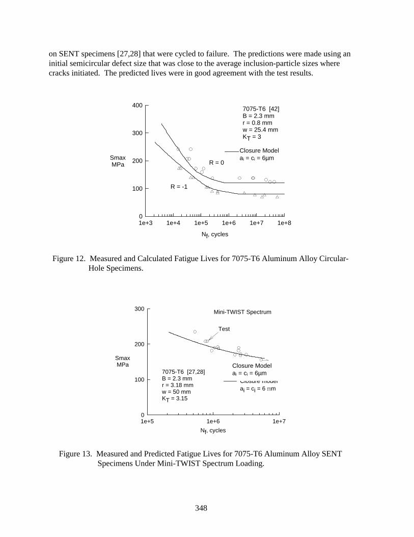
348
on SENT specimens [27,28] that were cycled to failure. The predictions were made using aninitial semicircular defect size that was close to the average inclusion-particle sizes wherecracks initiated. The predicted lives were in good agreement with the test results.
Nf, cycles
1e+3 1e+4 1e+5 1e+6 1e+7 1e+8
Smax MPa
0
100
200
300
4007075-T6 [42]B = 2.3 mmr = 0.8 mmw = 25.4 mmKT = 3
R = 0
R = -1
Closure modelai = ci = 6 mm
Figure 12. Measured and Calculated Fatigue Lives for 7075-T6 Aluminum Alloy Circular-Hole Specimens.
Nf, cycles
1e+5 1e+6 1e+7
Smax MPa
0
100
200
300
7075-T6 [27,28]B = 2.3 mmr = 3.18 mmw = 50 mmKT = 3.15
Closure modelai = ci = 6 mm
Mini-TWIST Spectrum
Test
Figure 13. Measured and Predicted Fatigue Lives for 7075-T6 Aluminum Alloy SENTSpecimens Under Mini-TWIST Spectrum Loading.
Closure Modelai = ci = 6µm
Closure Modelai = ci = 6µm
349
Titanium Alloy Ti-6Al-4V
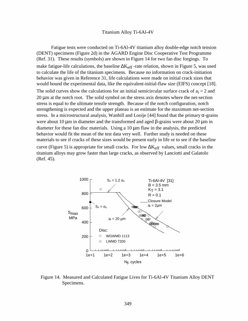
Fatigue tests were conducted on Ti-6Al-4V titanium alloy double-edge notch tension(DENT) specimens (Figure 2d) in the AGARD Engine Disc Cooperative Test Programme(Ref. 31). These results (symbols) are shown in Figure 14 for two fan disc forgings. To
make fatigue-life calculations, the baseline ∆Keff -rate relation, shown in Figure 5, was usedto calculate the life of the titanium specimens. Because no information on crack-initiationbehavior was given in Reference 31, life calculations were made on initial crack sizes thatwould bound the experimental data, like the equivalent-initial-flaw size (EIFS) concept [18].
The solid curves show the calculations for an initial semicircular surface crack of ai = 2 and20 µm at the notch root. The solid symbol on the stress axis denotes where the net-sectionstress is equal to the ultimate tensile strength. Because of the notch configuration, notchstrengthening is expected and the upper plateau is an estimate for the maximum net-sectionstress. In a microstructural analysis, Wanhill and Looije [44] found that the primary α-grainswere about 10 µm in diameter and the transformed and aged β-grains were about 20 µm indiameter for these fan disc materials. Using a 10 µm flaw in the analysis, the predictedbehavior would fit the mean of the test data very well. Further study is needed on thesematerials to see if cracks of these sizes would be present early in life or to see if the baseline
curve (Figure 5) is appropriate for small cracks. For low ∆Keff values, small cracks in thetitanium alloys may grow faster than large cracks, as observed by Lanciotti and Galatolo(Ref. 45).
1e+1 1e+2 1e+3 1e+4 1e+5 1e+60
200
400
600
800
1000
Smax MPa
Nf, cycles
Sn = 1.2 su Ti-6Al-4V [31]B = 3.5 mmKT = 3.1R = 0.1
Closure modelai = 2 mm
ai = 20 mm
Disc:WGWMD 1113
LWMD 7200
Sn = su
Figure 14. Measured and Calculated Fatigue Lives for Ti-6Al-4V Titanium Alloy DENTSpecimens.
Closure Modelai = 2µmSn = σu
ai = 20 µm
Sn = 1.2 σu
350
Steel 4340
Swain et al. [29] conducted fatigue and small-crack tests on 4340 steel single-edgenotch tension specimens. These tests were conducted under both constant-amplitude andspectrum loading. Inspection of fatigue surfaces showed that in each case a crack hadinitiated at an inclusion particle defect. The initiation site was either at a spherical (calcium-aluminate) or a stringer (manganese sulfide) inclusion particle. Examination of initiationsites for over 30 fatigue cracks produced information on the distribution of crack initiationsite dimensions. The spherical particle defects range in size from 10 to 40 µm in diameter.The stringer particles were typically 5 to 20 µm in the thickness direction and range up to 60
µm in the width direction. The median values of the defect dimensions measured were ai = 8
µm and ci = 13 µm. An equivalent area (semicircular) defect is 10 µm. This initial defectsize will be used later to predict fatigue lives.
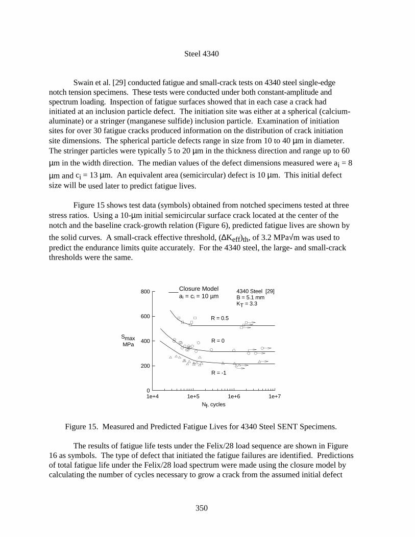
Figure 15 shows test data (symbols) obtained from notched specimens tested at threestress ratios. Using a 10-µm initial semicircular surface crack located at the center of thenotch and the baseline crack-growth relation (Figure 6), predicted fatigue lives are shown by
the solid curves. A small-crack effective threshold, (∆Keff)th, of 3.2 MPa√m was used topredict the endurance limits quite accurately. For the 4340 steel, the large- and small-crackthresholds were the same.
Nf, cycles1e+4 1e+5 1e+6 1e+7
Smax MPa
0
200
400
600
800 4340 Steel [29]B = 5.1 mmKT = 3.3
Closure modelai = ci = 10 mm
R = 0.5
R = 0
R = -1
Figure 15. Measured and Predicted Fatigue Lives for 4340 Steel SENT Specimens.
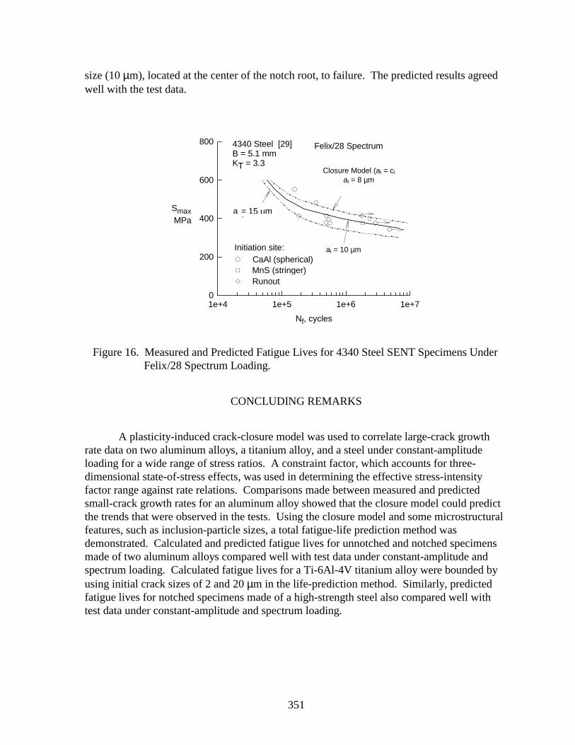
The results of fatigue life tests under the Felix/28 load sequence are shown in Figure16 as symbols. The type of defect that initiated the fatigue failures are identified. Predictionsof total fatigue life under the Felix/28 load spectrum were made using the closure model bycalculating the number of cycles necessary to grow a crack from the assumed initial defect
Closure Modelai = ci = 10 µm
351
size (10 µm), located at the center of the notch root, to failure. The predicted results agreedwell with the test data.
Nf, cycles
1e+4 1e+5 1e+6 1e+7
Smax MPa
0
200
400
600
800
Initiation site:CaAl (spherical)MnS (stringer)
4340 Steel [29]B = 5.1 mmKT = 3.3
Runout
Closure model (ai = ci)
ai = 10 mm
ai = 8 mm
ai = 15 mm
Felix/28 Spectrum
Figure 16. Measured and Predicted Fatigue Lives for 4340 Steel SENT Specimens UnderFelix/28 Spectrum Loading.
CONCLUDING REMARKS
A plasticity-induced crack-closure model was used to correlate large-crack growthrate data on two aluminum alloys, a titanium alloy, and a steel under constant-amplitudeloading for a wide range of stress ratios. A constraint factor, which accounts for three-dimensional state-of-stress effects, was used in determining the effective stress-intensityfactor range against rate relations. Comparisons made between measured and predictedsmall-crack growth rates for an aluminum alloy showed that the closure model could predictthe trends that were observed in the tests. Using the closure model and some microstructuralfeatures, such as inclusion-particle sizes, a total fatigue-life prediction method wasdemonstrated. Calculated and predicted fatigue lives for unnotched and notched specimensmade of two aluminum alloys compared well with test data under constant-amplitude andspectrum loading. Calculated fatigue lives for a Ti-6Al-4V titanium alloy were bounded byusing initial crack sizes of 2 and 20 µm in the life-prediction method. Similarly, predictedfatigue lives for notched specimens made of a high-strength steel also compared well withtest data under constant-amplitude and spectrum loading.
Closure Model (ai = ci
ai = 8 µm
ai = 10 µm
ai= 15 µm

352
ACKNOWLEDGMENT
The authors take this opportunity to thank our colleagues, Drs. Peter Edwards and X. R.Wu, for their leadership in the AGARD Structures and Materials Panel Short-Crack Programmeand the NASA/CAE Cooperative Program on Fatigue and Fracture Mechanics, respectively.Their guidance, and the efforts of the many participants in both programs, have contributed tomaking Small-Crack Theory successful.
NOMENCLATURE
a Crack length in thickness (B) direction, mmai Initial defect or crack length in B-direction, mmb Defect or void half height, mmB Specimen thickness, mmc Crack length in width (w) direction, mmci Initial defect or crack length in w-direction, mmF Boundary-correction factorKF Elastic-plastic fracture toughness in TPFC, MPa√mm Fracture toughness parameter in TPFCN Number of cyclesNf Number of cycles to failureR Stress ratio (Smin/Smax)r Notch or hole radius, mmS Applied stress, MPaS′o Crack-opening stress, MPaSmax Maximum applied stress, MPaSmin Minimum applied stress, MPaw Specimen width or half width (see Figure 2), mmα Constraint factor∆K Stress-intensity factor range, MPa√m∆Keff Effective stress-intensity factor range, MPa√m(∆Keff)T Effective stress-intensity factor range, MPa√m(∆Keff)th Small crack ∆Keff threshold, MPa√m∆Kth Large crack ∆K threshold, MPa√mρ Plastic-zone size, mmσo Flow stress (average of σys and σu), MPaσys Yield stress (0.2 percent offset), MPaσu Ultimate tensile strength, MPaω Cyclic-plastic-zone size, mm
353
REFERENCES
1. Pearson, S., “Initiation of Fatigue Cracks in Commercial Aluminum Alloys and theSubsequent Propagation of Very Short Cracks,” Engineering Fracture Mechanics,Vol. 7, No. 2, 1975, pp. 235-247.
2. Ritchie, R. O. and Lankford, J., eds., Small Fatigue Cracks, The MetallurgicalSociety, Inc., Warrendale, PA, 1986.
3. Miller, K. J. and de los Rios, E. R., eds., The Behaviour of Short Fatigue Cracks,European Group on Fracture, Publication No. 1, 1986.
4. Zocher, H., ed., Behaviour of Short Cracks in Airframe Components, AGARDCP-328, 1983.
5. Newman, J. C., Jr. and Edwards, P. R., “Short-Crack Growth Behaviour in anAluminum Alloy - An AGARD Cooperative Test Programme,” AGARD R-732,1988.
6. Edwards, P. R. and Newman, J. C., Jr., eds., Short-Crack Growth Behaviour inVarious Aircraft Materials, AGARD Report No. 767, 1990.
7. Raju, I. S. and Newman, J. C., Jr., “Stress-Intensity Factors for a Wide Range ofSemi-Elliptical Surface Cracks in Finite-Thickness Plates,” Engineering FractureMechanics, Vol. 11, No. 4, 1979, pp. 817-829.
8. Newman, J. C., Jr. and Raju, I. S., “Stress-Intensity Factor Equations for Cracks inThree-Dimensional Finite Bodies,” ASTM STP 791, Vol. I, 1983, pp. 238-265.
9. El Haddad, M., Dowling, N., Topper, T., and Smith, K., “J Integral Application forShort Fatigue Cracks at Notches,” International Journal of Fracture, Vol. 16, 1980,pp. 15-30.
10. Newman, J. C., Jr., “Fracture Mechanics Parameters for Small Fatigue Cracks,” SmallCrack Test Methods, ASTM STP 1149, J. Allison and J. Larsen, eds., 1992, pp. 6-28.
11. Leis, B., Kanninen, M., Hopper, A., Ahmad, J., and Broek, D., “Critical Review ofFatigue Growth of Short Cracks,” Engineering Fracture Mechanics, Vol. 23, 1986,pp. 883-898.
12. Elber, W., “The Significance of Fatigue Crack Closure,” Damage Tolerance inAircraft Structures, ASTM STP 486, 1971, pp. 230-242.
13. Nisitani, H. and Takao, K. I., “Significance of Initiation, Propagation and Closure ofMicrocracks in High Cycle Fatigue of Ductile Materials,” Engineering FractureMechanics, Vol. 15, No. 3, 1981, pp. 455-456.
354
14. Minakawa, K. and McEvily, A. J., “On Near-Threshold Fatigue-Crack Growth inSteels and Aluminum Alloys,” Proceedings of the International Conference onFatigue Thresholds, Vol. 2, 1981, pp. 373-390.
15. Newman, J. C., Jr., “A Nonlinear Fracture Mechanics Approach to the Growth ofSmall Cracks,” Behaviour of Short Cracks in Airframe Components, H. Zocher, ed.,AGARD CP-328, 1983, pp. 6.1-6.26.
16. Newman, J. C., Jr., “A Crack-Closure Model for Predicting Fatigue-Crack Growthunder Aircraft Spectrum Loading,” Methods and Models for Predicting Fatigue CrackGrowth under Random Loading, J. Chang and C. Hudson, eds., ASTM STP 748,1981, pp. 53-84.
17. Newman, J. C., Jr., “A Crack-Opening Stress Equation for Fatigue Crack Growth,”International Journal of Fracture, Vol. 24, 1984, R131-R135.
18. Rudd, J., Yang, J., Manning, S., and Garver, W., “Durability Design Requirementsand Analysis for Metallic Airframes,” Design of Fatigue and Fracture ResistantStructures, ASTM STP 761, P. R. Abelkis and C. M. Hudson, eds., 1982, pp. 133-151.
19. van Dijk, G. and deJonge, J., “Introduction to a Fighter Loading Standard for FatigueEvaluationFALSTAFF,” NLR MP 75017 U, Nationaal Lucht-enRuimtevaartlaborium, 1975.
20. Huck, M., Schutz, W., Fischer, R., and Kobler, H. G., “A Standard Random LoadSequence of Gaussian Type Recommended for General Application in FatigueTesting,” IABG Report No. TF-570 or LBF Report No. 2909, Germany, 1976.
21. deJonge, J. B., Schutz, D., Lowak, H., and Schijve, J., “A Standardized LoadSequence for Flight Simulation Tests on Transport Aircraft Wing Structures(TWIST),” NLR TR-73029 U, Nationaal Lucht-en Ruimtevaartlaborium,Netherlands, 1973.
22. Lowak, H., deJonge, J. B., Franz, J., and Schutz, D., “Mini-TWISTA ShortenedVersion of TWIST,” LBF Report No. TB-146, Laboratorium fur Betriebsfestigkeit,Germany, 1979.
23. Edwards, P. R. and Darts, J., “Standardized Fatigue Loading Sequences for HelicopterRotors (Helix and Felix) - Part 2: Final Definition of Helix and Felix,” RAETechnical Report 84085, 1984.
24. Hudson, C. M., “Effect of Stress Ratio on Fatigue-Crack Growth in 7075-T6 and2024-T3 Aluminum Alloy Specimens,” NASA TN D-5390, 1969.
25. Phillips, E. P., “The Influence of Crack Closure on Fatigue-Crack Growth Thresholdsin 2024-T3 Aluminum Alloy,” ASTM STP 982, 1988, pp. 505-515.
355
26. Dubensky, R. G., “Fatigue Crack Propagation in 2024-T3 and 7075-T6 AluminumAlloys at High Stress,” NASA CR-1732, March 1971.
27. Newman, J. C., Jr., Wu, X. R., Swain, M. H., Zhao, W., Phillips, E. P., and Ding,C. F., “Small-Crack Growth Behavior in High-Strength Aluminum Alloys - ANASA/CAE Cooperative Program,” 18th Congress International Council ofAeronautical Sciences, Beijing, PRC, September 1992, pp. 799-820.
28. Newman, J. C., Jr., Wu, X. R., Venneri, S. L., and Li., C. G., “Small-Crack Effects inHigh-Strength Aluminum Alloys - A NASA/CAE Cooperative Program,” NASAReference Publication 1309, 1994.
29. Swain, M. H., Everett, R. A., Newman, J. C., Jr., and Phillips, E. P., “The Growth ofShort Cracks in 4340 Steel and Aluminum-Lithium 2090,” AGARD R-767, P. R.Edwards and J. C. Newman, Jr., eds., 1990, pp. 7.1-7.30.
30. Raizenne, M. D., “AGARD SMP Sub-Committee 33 Engine Disc Test ProgrammeFatigue-Crack Growth Rate Data and Modeling Cases for Ti-6Al-4V, IMI-685 andTi-17,” LTR-ST-1785, National Research Council, Canada, 1990.
31. Mom, A. J. A. and Raizenne, M. D., eds., AGARD Engine Disc Cooperative TestProgramme, AGARD Report No. 766, 1988.
32. Powell, B. E. and Henderson, I., “The Conjoint Action of High and Low CycleFatigue,” AFWAL-TR-83-4119, 1983.
33. Dugdale, D. S., “Yielding of Steel Sheets Containing Slits,” Journal of Mechanics andPhysics of Solids”, Vol. 8, No. 2, 1960, pp. 100-104.
34. Blom, A. F., Wang, G. S., and Chermahini, R. G., “Comparison of Crack ClosureResults Obtained by 3-D Elastic-Plastic FEM and Modified Dugdale Model,”Proceedings 1st International Conference on Computer Aided Assessment andControl of Localized Damage, Portsmouth, England, 1990, pp. 57-68.
35. Schijve, J., “Significance of Fatigue Cracks in Micro-Range and Macro-Range,”Fatigue Crack Propagation, ASTM STP 415, 1967, pp. 415-459.
36. Newman, J. C., Swain, M. H., and Phillips, E. P., “An Assessment of the Small-CrackEffect for 2024-T3,” Small Fatigue Cracks, R. Ritchie and J. Lankford, eds., 1986,pp. 427-452.
37. Newman, J. C., Jr., “FASTRAN IIA Fatigue Crack Growth Structural AnalysisProgram,” NASA TM 104159, 1992.
38. Newman, J. C., Jr., “Effects of Constraint on Crack Growth under Aircraft SpectrumLoading,” Fatigue of Aircraft Materials, A. Beukers et al., eds., Delft UniversityPress, 1992, pp. 83-109.
356
39. Newman, J. C., Jr., “Fracture Analysis of Various Cracked Configurations in Sheetand Plate Materials,” ASTM STP 605, 1976, pp. 104-123.
40. Lankford, J., “The Growth of Small Fatigue Cracks in 7075-T6 Aluminum,” Fatigueof Engineering Materials and Structures, Vol. 5, 1982, pp. 233-248.
41. Grover, H. J., Hyler, W. S., Kuhn, P., Landers, C. B., and Howell, F. M., “Axial-LoadFatigue Properties of 24S-T and 75S-T Aluminum Alloy as Determined in SeveralLaboratories,” NACA TN-2928, 1953.
42. Landers, C. B. and Hardrath, H. F., “Results of Axial-Load Fatigue Tests onElectropolished 2024-T3 and 7075-T6 Aluminum Alloy Sheet Specimens withCentral Holes,” NACA TN-3631, 1956.
43. Bowles, C. Q. and Schijve, J., “The Role of Inclusions in Fatigue Crack Initiation inan Aluminum Alloy,” International Journal of Fracture, Vol. 9, No. 2, 1973,pp. 171-179.
44. Wanhill, R. J. H. and Looije, C. E. W., “Fractographic and Microstructural Analysisof Fatigue Crack Growth in Ti-6Al-4V Fan Disc Forgings,” AGARD Engine DiscCooperative Test Programme, T. Pardessus, E. Jany, and M. D. Raizenne, eds.,AGARD Report 766 (addendum), 1993, pp. 2.1-2.88.
45. Lanciotti, A. and Galatolo, R., “Short Crack Observations in Ti-6Al-4V UnderConstant-Amplitude Loading”, Short-Crack Growth Behaviour in Various AircraftMaterials, P. R. Edwards and J. C. Newman, Jr., eds., AGARD R-767, 1990,pp. 10.1-10.7.
357
FULL-SCALE GLARE FUSELAGE PANEL TESTS1
Roland W. A. Vercammen and Harold H. OttensNational Aerospace Laboratory (NLR)
Amsterdam, The Netherlands
SUMMARY
A GLARE fuselage panel, representative of the crown section of the Fokker 100fuselage just in front of the wing, has been tested in the curved fuselage panel test facility thatwas recently commissioned at the National Aerospace Laboratory (NLR). Panels are loadedby internal air pressure resulting in tangential stresses in the panel and by axial loadingrepresentative of both the cabin pressure and the fuselage bending due to taxiing and gustloading. A fatigue test was performed in which 180,000 flights (two lifetimes) weresimulated. After the fatigue test no damage was observed. The fatigue test was followed bystatic tests to limit load and to ultimate load. Finally the panel was loaded to failure at 1.32ultimate load. This paper will describe the test setup in some detail, demonstrate the obtaineduniform strain distribution in the panel, show the fatigue loads applied at high test frequency,and present the results of the GLARE fuselage panel tests which proof that the use ofGLARE leads to a substantial weight reduction without affecting the fatigue or staticstrength.
INTRODUCTION
In fuselage design studies there will always be the necessity to test components in arealistic way. The fuselage panel test facility developed and built at the National AerospaceLaboratory (NLR) (fig. 1) offers the possibility to test fuselage skin sections, with curvaturesranging from panels of relatively small aircraft like the Fokker 50 to panels from relativelylarge aircraft like the Airbus A300, at a high fatigue testing speed (ref. 1). The fatigue testloads simulate flight simulation loading conditions by loads in circumferential directioncaused by cabin pressurization and axial loads representative of both the cabin pressure andthe fuselage bending due to taxiing and gust loading. The new fuselage panel test facility hasalso the possibility to perform static strength and residual strength tests.
In order to verify the applicability of GLARE A2 as a fuselage skin material Fokkerdesigned and built a Fokker 100 fuselage panel with a GLARE A skin and GLARE N
1 This investigation has been carried out under a contract awarded by Fokker Aircraft B.V. according to the
commitments made by Fokker in the Brite Euram IMT 2040 project “Fibre reinforced metal laminates andCFRP fuselage concepts.”
358
stringers, representative of the crown section just in front of the wing. GLARE A as skinmaterial is weight favorable compared to GLARE C when the amount of necessary doublersfor countersunk riveting is restricted to only doublers in the axial lapjoints. In the frame-skinattachments no doublers were required as the frames were connected to the stringers bymeans of cleats instead of to the skin by means of castellations as is normally done byFokker. Applying cleats led to a panel design with a threefold test objective:
• Verification of the applicability of GLARE A as a fuselage skin material for loadingconditions which are representative of the crown section of the Fokker 100 fuselage.
• Generation of test evidence on the static strength and fatigue behavior of rigidstringer-frame attachments in the GLARE fuselage.
• Determining the deterioration of the static strength of the GLARE skin after twotimes the design life (2 × 90,000 flights).
The overall panel dimensions are 1210 mm × 3030 mm containing five aluminum frameswith a pitch of 500 mm, seven stringers with a pitch of 147 mm, seven stringers couplingsand a longitudinal riveted lap joint in the panel center (fig. 2). One of the frames is a Z-shaped frame, the others are C-shaped frames. A complete top section made of GLARE Awith GLARE N stringers and rigid stringer-frame attachments has a weight that is 63 percentof the current Fokker 100 design in aluminum (ref. 2).
TEST FACILITY
Fuselage skins of most aircraft are subjected to biaxial loads, owing to bending andpressurization of the fuselage. In evaluating damage tolerance properties of candidatefuselage structures and materials, it is highly desirable that curved structures are tested underbiaxial loading conditions. For this purpose one generally uses a barrel test setup. This is afull-size cylindrical pressure vessel consisting of several interconnected fuselage panels. Abarrel test setup, however, has some features which make it less flexible and therefore lessattractive for studies not directly related to a particular aircraft design. The radius ofcurvature is fixed, a large number of panels have to be tested simultaneously and the testfrequency is rather low. In addition, barrel tests are expensive due to the large number ofpanels and the long testing time. The panel test facility at NLR was developed to avoid theaforementioned disadvantages. In the curved fuselage panel test facility, which has flexibilitywith regard to panel diameter, panel width, and panel length, a single fuselage panel can betested at a relatively high testing speed.
2 ).ARE A=GLARE 3-2/1-0.3: 2×(0.3 mm 2024 sheet) + (0.25 mm cross-ply glass prepreg)
GLARE N=GLARE 1-3/2-0.3: 3×(0.3 mm 7475 sheet) + 2×(0.25 mm UD glass prepreg)GLARE C=GLARE 3-3/2-0.2: 3×(0.2 mm 2024 sheet) + 2×(0.25 mm cross-ply glass prepreg)

359
The major components of the test facility are the main frame, the pressure chamber,and the load introduction systems (fig. 1). The main frame is a very stiff steel structure. Itconsists of heavy bottom and top beams and two vertical main columns. A pyramidal shapedframe, which houses the hydraulic actuator, is mounted above the top beam and two auxiliaryvertical columns. The panel is mounted in the frame such that the center of gravity of itscross section is in the working line of the actuator. The height of the test facility is about 7.2m; the width is about 4.5 m. The pressure chamber is formed by a seal and base structureconnected to a transport system. The base structure of the pressure chamber is formed by astiffened base plate and two support beams which are bolted to the vertical columns of themain structure. The base plate has a large central hole for air supply. At the front side thebase plate has curved wooden blocks around the edges which form the side walls of thepressure chamber. An inflatable inner seal is mounted on the wooden blocks and the pressurechamber is closed by the panel. In order to accomplish an air-tight seal without net radialforce acting on the panel edges, an inflatable outer seal is mounted at the outside of the paneljust opposite the inner seal. The outer seal is bonded on the reaction frame, which consists ofan open rectangular steel frame with curved wooden blocks. With the transport system thepressure chamber can easily be shifted aside during the test, which significantly improves theinspectability of the test panel. The chamber pressurization, axial loads, and sealpressurization are regulated by a control system.
Pressurization of the fuselage panel is reacted to the test frame leading to tangentialstresses in the skin and normal stresses in the frames. The ratio of the stresses in the skin andframes is determined and can be adjusted by the stiffness ratio of the skin-to-testframe andframe-to-testframe connections. The tangential stresses in the skin are taken out by bondedglass fibers. The loads in the frames are transferred to steel rods. Therefore the ends of thepanel frames are locally reinforced. The wooden blocks have several holes through which thepanel frame tensile rods are guided. The openings between the panel frame tensile rods andthe hole edges are sealed air-tight with silicone rubber collars. In axial direction the panelends are loaded by rods which are connected to the panel ends by steel brackets. At theseaxial panel ends the stringers are ended and the stringers loads are taken by a graduallyincreased skin thickness (fig. 2). This makes it possible to seal directly on the skin of thepanel.
The advantages of using unidirectional glass fibers is that the loads are very evenlyintroduced over the length of the panel (ref. 3). Therefore hardly any distance is required forstress redistribution, i.e., the stress distribution is uniform at a very small distance from thepanel edge. In addition, the use of unidirectional fibers does not result in local stiffening ofthe panel edges in axial direction. The length of the glass fiber sheets was chosen sufficientlylarge to limit the rotation of the fibers at the upper side of the panel owing to axial elongationof the panel. The small rotation that occurs during the test does not significantly alter theload transfer through the panel. The glass fibers are bonded to steel tangential plates. Because of their large width, the tangential plates act more or less as hinges. The outwardmovement of the panel due to pressurization is therefore nearly radial and will not result in asignificant change in the shape of the panel from circular to oval. The tangential clamping
360
system was designed such that the angle between tangential plates and the vertical columnwas adjustable to allow for a large range of panel diameters to be tested.
PANEL LOADS
The GLARE panel is designed for the Fokker 100 loads in the crown section atFuselage Station 14911. The axial loading sequences of the fatigue spectrum are derivedfrom the spectrum applied in the Fokker 100 full-scale test (ref. 4). The axial load is writtenas
Faxial= a1 × My + a2 ×∆Rwith
Faxial=axial load in fuselage panel/[= bending moment at Fuselage Station 14911∆R= cabin pressureC= Fuselage Station dependent constants
The spectrum consists of 36 repeating testblocks of 5000 flights. Each testblock of 5000flights is subdivided in four subblocks of 1250 flights. Three subblocks are exactly equal; thefourth block is equal but for one severe flight. Within this spectrum eight flight types withdifferent gust loading severity have been defined. Figure 3 shows the axial loading andfrequency per 5000 flights for these typical eight flight types. Each flight has five segments:ground, initial climb, climb/descent, cruise, and approach. During the groundsegments thecabin pressure∆R = zero, during the cruise segment∆R =∆ROCZIn case of climb/descent thecabin pressure varies between zero and ∆ROCZ
The fatigue test is followed by static tests. The GLARE panel is subjected to onelimit load case, two ultimate load cases, and a failure strength test. These static load casesare intended to demonstrate that after two times the design life (2 × 90,000 flights) andpossible undetectable cracks in the GLARE skin the residual strength is still sufficient tocarry limit and ultimate load. The limit load case equals cabin pressure∆R= ∆ROCZplus limitload bending moment. The first ultimate load case is the cabin pressure ultimate load case:
∆R=2 ×∆ROCZ. The second ultimate load case equals 1.5 × [cabin pressure∆R=∆ROCZ pluslimit load bending moment]. The second ultimate load case is followed by the failurestrength test at∆R=∆ROCZby increasing the axial load until failure of the panel.
STRAIN DISTRIBUTION
At fastening of a test panel, the length of each axial tensile rod and frame loading rodcan be adjusted with nut keys such that over the panel width and length a uniform strain orstress distribution is achieved when the panel is loaded. The amount of load thatKU taken outof the panel frames also depends on the stiffness of the rods. The rods are therefore panel
361
dependent parts and have load cells incorporated. The nut keys and the output of the loadcell in each panel frame can be used for proper adjustments.
The strain distribution in the middle of the panel, obtained by using the glass fibers,frame loading rods in tangential direction, and tensile rods at the reinforced, nonstiffenedpanel ends in axial direction, is shown in figures 4 and 5. These graphs visualize a smoothdistribution of the axial and tangential strain levels and a uniform tangential straindistribution within 100 mm of the panel edges loaded with glass fibers. Strain levelvariations at the gauges R13a, R14c, and R16a are due to the lap-joint, radius differences ofpanel halves, and stringer couplings. The tangential strain distribution over the panel lengthis given in figure 6. Over the panel width the influence of the stringers run-outs and skinreinforcements are negligible after the first frame (fig. 7).
At constant bending moment (Faxbending = constant), the radial expansion of the panelincreased due to raising cabin pressure. When, at constant cabin pressure(Fax∆R=constant),the axial force was raised the radial expansion of the panel decreased. The panel displacedinwards to the pressure chamber to resist the increasing tangential contraction due to thePoisson's ratio effect due to the axial extension. The increase of the tangential contractionand the displacement of the panel inwards led to a decrease of the tangential strains in theskin.
FATIGUE TEST
During the fatigue test the defined 180,000 flights were applied. The testingfrequency was about 10,000 flights per 24 hours. The axial loads had an accuracy of 0.5percent, the chamber pressure reproduced within 3 percent. The panel was inspected by eddycurrent at the axial lap joint and stringer run-outs and checked visually at the stringercouplings, doubler run-outs, stringers at the connection with the cleats, frames at theconnection with the cleats, and load introduction points of the frames. In accordance with thelifetime predictions (ref. 2) no cracks or damages were found.
STATIC TESTS
The fatigue test was followed by static tests. The first static load case was the limitload test. For this load case, figure 7 gives the axial strain levels from station zero till thefourth frame. Clearly visible is the pillowing of the skin. The lower axial strains in thesecond and third bay are caused by the stringer couplings and the difference in stiffnesses ofthe frames. During this limit load test the panel extended linearly, and no permanentdeformations took place. Some results of the first ultimate load case at2×∆Rare visualizedin figure 5. Figure 5 shows the tangential strain levels in the middle of the panel. The axialstrain levels are less than 20 percent of the tangential levels. Like during the limit load, test
362
pillowing occurred and the panel expanded linearly without permanent deformations. Afterthe 2 ×∆Rultimate load case, the second ultimate load test was applied. No final failureoccurred and the strain distribution was, except for plasticity which occurred above limitload, conformed to the distribution during the limit load test. Conclusion: the ultimate loadtests showed sufficient residual strength of the GLARE panel after two lifetimes of fatigueloading.
To determine the deterioration of the panel after two lifetimes of fatigue loading, thefirst few load steps of the limit load and ultimate load tests were compared with referencetests performed before the fatigue test. The deterioration of strain levels in the axial directionwas a small fixed value of 50zstrain caused by settling of the brackets, doublers, and rivets. In the tangential direction negligible differences (< 1.0 percent) were noticed.
After the second ultimate load test, the cabin pressure was fixed at∆R =∆ROCZand thepanel was axially loaded to failure. The axial strains are visualized in figure 8. Failureoccurred at an axial load of 770 kN, i.e., 1.32 × axial ultimate load. This axial load is 15percent higher than the theoretically expected axial failure load (ref. 2). The skin failedbetween the third and fourth frame at the cross section of the last rivets of the stringerscouplings (fig. 9). Conclusion: in the crown section of the Fokker 100, GLARE A asfuselage skin material and GLARE N as stringer material are applicable. The skin, lap joint,and rigid stringer frame attachments (cleats) had enough fatigue and static strength.
CONCLUSIONS
The new full-scale fuselage panel test facility operated correctly. The loadintroduction in the panel in axial and tangential direction was uniform and realistic fatigueloads due to cabin pressure and fuselage bending could be applied at high frequency (10,000flights per 24 hours).
The conclusions with regard to the Fokker GLARE panel are:
• No cracks were found in lap joints, cleats, stringers, skin, frames, and stringercouplings after the two lifetimes fatigue test (inspection was done visually and byeddy current).
• The panel as a whole did not permanently deform at limit load.
• In both ultimate load test cases, no failure occurred.
• Final failure occurred at 1.32 × axial ultimate load, which is 15 percent higher thantheoretically expected.
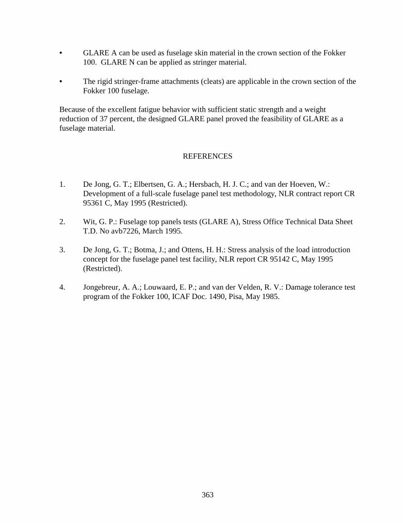
363
• GLARE A can be used as fuselage skin material in the crown section of the Fokker100. GLARE N can be applied as stringer material.
• The rigid stringer-frame attachments (cleats) are applicable in the crown section of theFokker 100 fuselage.
Because of the excellent fatigue behavior with sufficient static strength and a weightreduction of 37 percent, the designed GLARE panel proved the feasibility of GLARE as afuselage material.
REFERENCES
1. De Jong, G. T.; Elbertsen, G. A.; Hersbach, H. J. C.; and van der Hoeven, W.:Development of a full-scale fuselage panel test methodology, NLR contract report CR95361 C, May 1995 (Restricted).
2. Wit, G. P.: Fuselage top panels tests (GLARE A), Stress Office Technical Data Sheet
T.D. No avb7226, March 1995. 3. De Jong, G. T.; Botma, J.; and Ottens, H. H.: Stress analysis of the load introduction
concept for the fuselage panel test facility, NLR report CR 95142 C, May 1995(Restricted).
4. Jongebreur, A. A.; Louwaard, E. P.; and van der Velden, R. V.: Damage tolerance test
program of the Fokker 100, ICAF Doc. 1490, Pisa, May 1985.
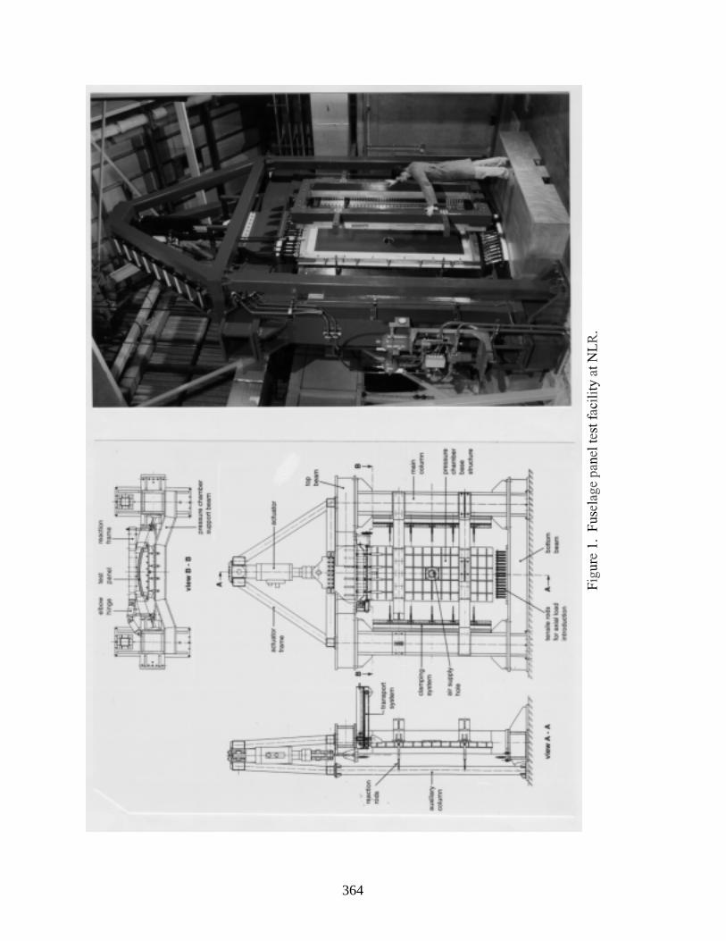
364
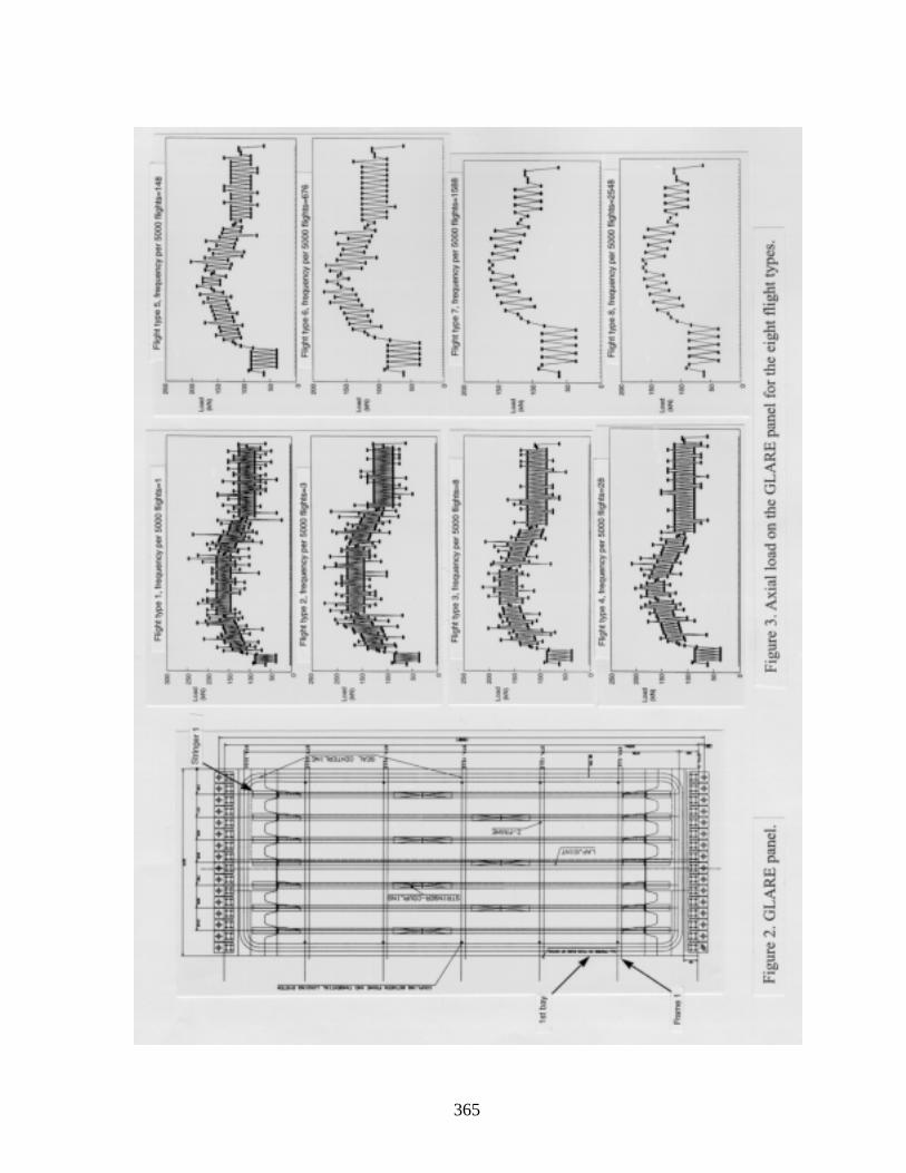
365
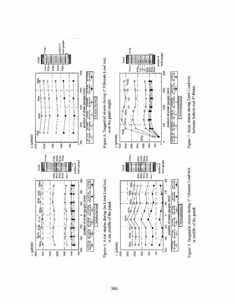
366
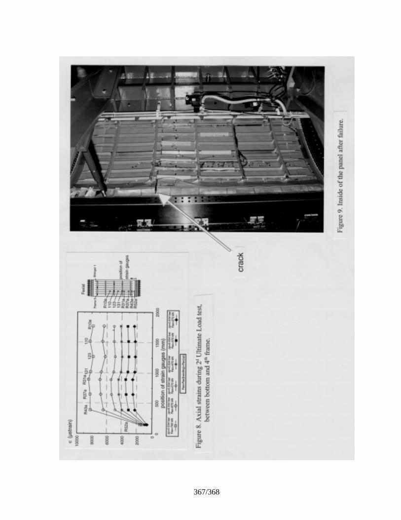
367/368
369
A GRAPHIC USER INTERFACE (GUI) FRONT-END FORPARAMETRIC SURVEY AND ITS APPLICATION TO
COMPOSITE PATCH REPAIRS OF METALLIC STRUCTURE
H. Kawai, H. Okada, and S. N. AtluriFAA Center of Excellence for
Computational Modeling of Aircraft StructuresGeorgia Institute of Technology
Atlanta, GA 30332-0356
SUMMARY
A graphical user interface (GUI) front-end program Parametric Survey (ParS) hasbeen developed on Microsoft Windows NT and Windows 95. It supports the parametricsurvey of analyses. In a parametric survey, a series of analyses of the same kind areperformed with different input parameter sets, and multiple output parameter sets arecollected. The data are visualized as charts which show the relationship between input andoutput parameters. Using ParS, a user can perform a parametric survey effectively through itsautomation of analyses and visualization functionality.
ParS is applied to a composite patch repair problem of aircraft fuselage. In thisproblem, a crack exists in a pressurized fuselage of an aircraft. Analyses for the effectivenessof the adhesive bonded composite repair were carried out. Some results of the analyses arepresented.
INTRODUCTION
A Graphical User Interface (GUI) front-end program ParS (Parametric Survey) hasbeen developed on Microsoft Windows NT and Windows 95 operating systems. It supportsparametric survey of analyses. Figure 1 describes the typical sequences of a parametricsurvey.
An analysis, such as a simulation of structural mechanics, fluid dynamics, chemicalreaction, or molecular dynamics requires a huge number of input data and generates a hugeamount of output data. When an engineer has to solve more specific problems, such as cracksin aircraft fuselage or a flow field behind a car, these analyses are represented typically by afew key input and output parameters from the engineer’s point of view. For example, in thecase of the structural integrity analysis for an aircraft fuselage (with cracks), one needs tospecify a few key input parameters such as the length of the crack, size of the fuselage model,and material properties. Other input data for the analysis program can be generated
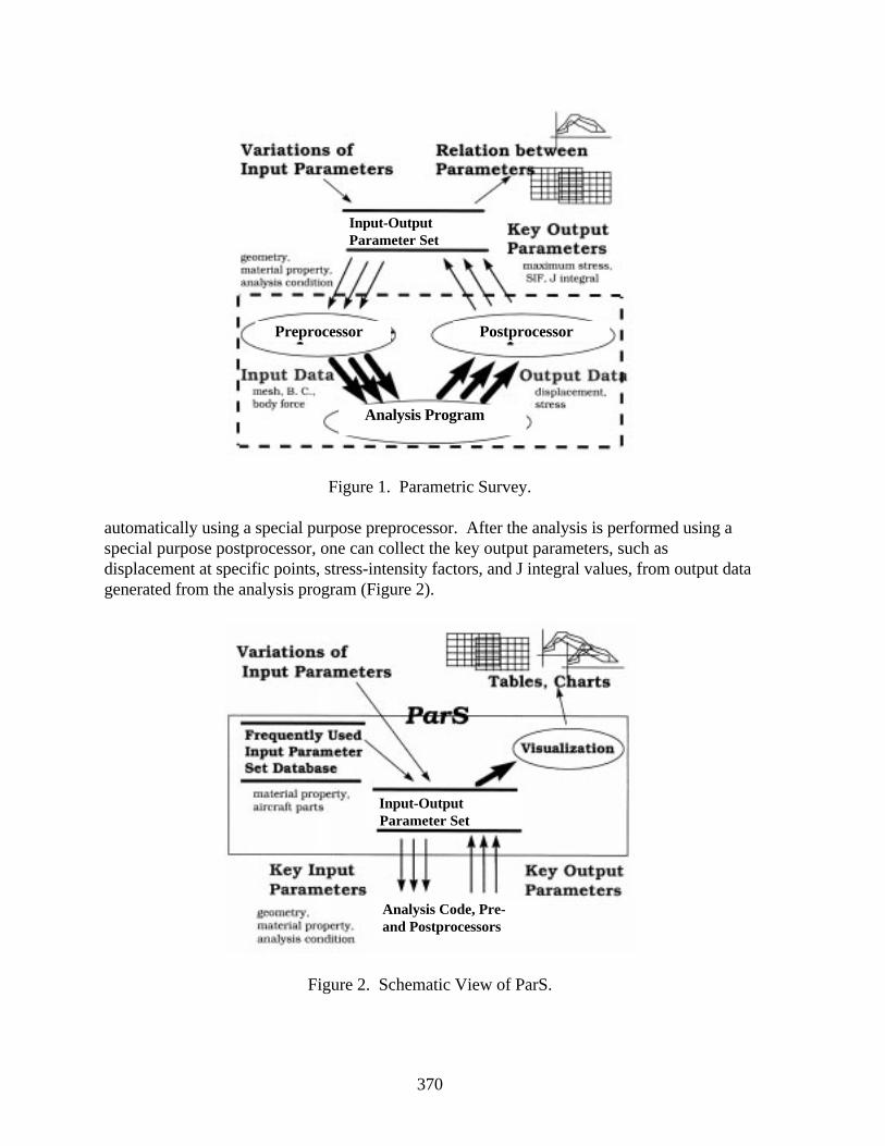
370
Figure 1. Parametric Survey.
automatically using a special purpose preprocessor. After the analysis is performed using aspecial purpose postprocessor, one can collect the key output parameters, such asdisplacement at specific points, stress-intensity factors, and J integral values, from output datagenerated from the analysis program (Figure 2).
Figure 2. Schematic View of ParS.
Input-OutputParameter Set
Input-Output Parameter Set
Preprocessor
Analysis Code, Pre- and Postprocessors
Postprocessor
Analysis Program
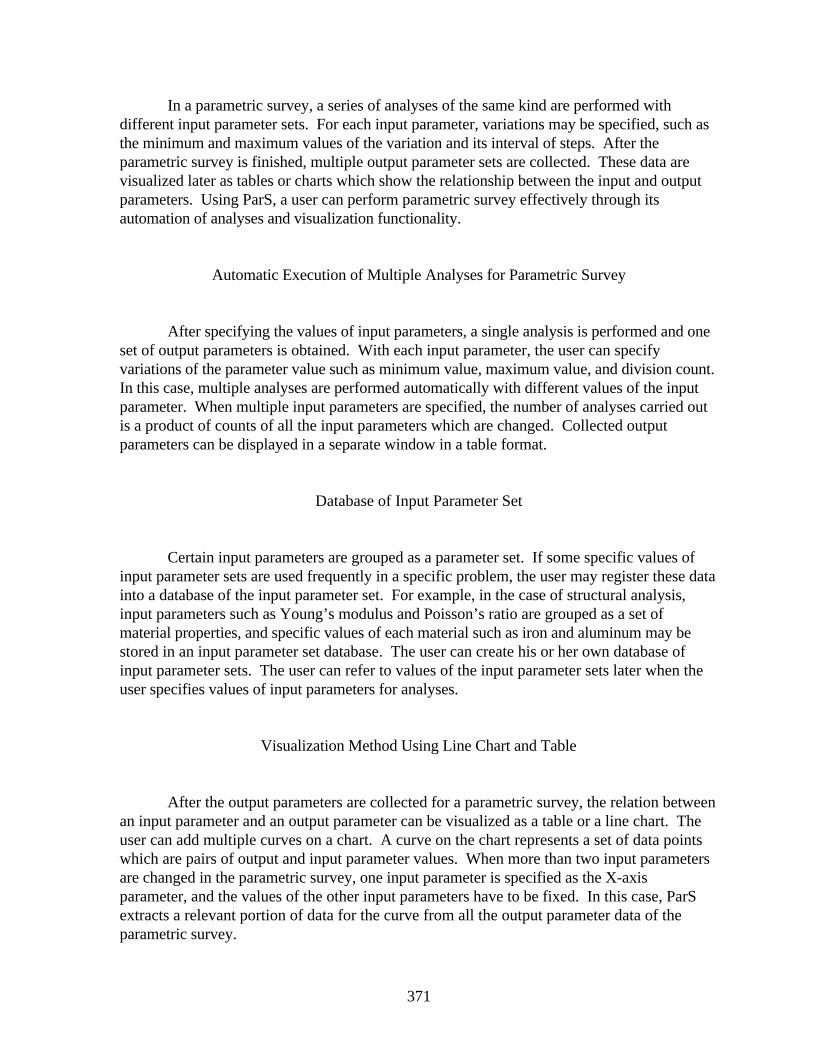
371
In a parametric survey, a series of analyses of the same kind are performed withdifferent input parameter sets. For each input parameter, variations may be specified, such asthe minimum and maximum values of the variation and its interval of steps. After theparametric survey is finished, multiple output parameter sets are collected. These data arevisualized later as tables or charts which show the relationship between the input and outputparameters. Using ParS, a user can perform parametric survey effectively through itsautomation of analyses and visualization functionality.
Automatic Execution of Multiple Analyses for Parametric Survey
After specifying the values of input parameters, a single analysis is performed and oneset of output parameters is obtained. With each input parameter, the user can specifyvariations of the parameter value such as minimum value, maximum value, and division count.In this case, multiple analyses are performed automatically with different values of the inputparameter. When multiple input parameters are specified, the number of analyses carried outis a product of counts of all the input parameters which are changed. Collected outputparameters can be displayed in a separate window in a table format.
Database of Input Parameter Set
Certain input parameters are grouped as a parameter set. If some specific values ofinput parameter sets are used frequently in a specific problem, the user may register these datainto a database of the input parameter set. For example, in the case of structural analysis,input parameters such as Young’s modulus and Poisson’s ratio are grouped as a set ofmaterial properties, and specific values of each material such as iron and aluminum may bestored in an input parameter set database. The user can create his or her own database ofinput parameter sets. The user can refer to values of the input parameter sets later when theuser specifies values of input parameters for analyses.
Visualization Method Using Line Chart and Table
After the output parameters are collected for a parametric survey, the relation betweenan input parameter and an output parameter can be visualized as a table or a line chart. Theuser can add multiple curves on a chart. A curve on the chart represents a set of data pointswhich are pairs of output and input parameter values. When more than two input parametersare changed in the parametric survey, one input parameter is specified as the X-axisparameter, and the values of the other input parameters have to be fixed. In this case, ParSextracts a relevant portion of data for the curve from all the output parameter data of theparametric survey.
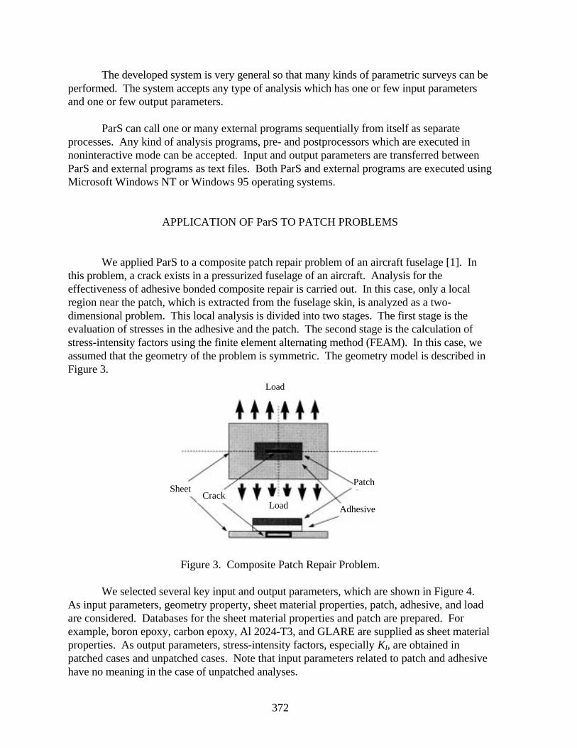
372
The developed system is very general so that many kinds of parametric surveys can beperformed. The system accepts any type of analysis which has one or few input parametersand one or few output parameters.
ParS can call one or many external programs sequentially from itself as separateprocesses. Any kind of analysis programs, pre- and postprocessors which are executed innoninteractive mode can be accepted. Input and output parameters are transferred betweenParS and external programs as text files. Both ParS and external programs are executed usingMicrosoft Windows NT or Windows 95 operating systems.
APPLICATION OF ParS TO PATCH PROBLEMS
We applied ParS to a composite patch repair problem of an aircraft fuselage [1]. Inthis problem, a crack exists in a pressurized fuselage of an aircraft. Analysis for theeffectiveness of adhesive bonded composite repair is carried out. In this case, only a localregion near the patch, which is extracted from the fuselage skin, is analyzed as a two-dimensional problem. This local analysis is divided into two stages. The first stage is theevaluation of stresses in the adhesive and the patch. The second stage is the calculation ofstress-intensity factors using the finite element alternating method (FEAM). In this case, weassumed that the geometry of the problem is symmetric. The geometry model is described inFigure 3.
Figure 3. Composite Patch Repair Problem.
We selected several key input and output parameters, which are shown in Figure 4.As input parameters, geometry property, sheet material properties, patch, adhesive, and loadare considered. Databases for the sheet material properties and patch are prepared. Forexample, boron epoxy, carbon epoxy, Al 2024-T3, and GLARE are supplied as sheet materialproperties. As output parameters, stress-intensity factors, especially KI, are obtained inpatched cases and unpatched cases. Note that input parameters related to patch and adhesivehave no meaning in the case of unpatched analyses.
SheetPatch
Load
Load
Crack
Adhesive
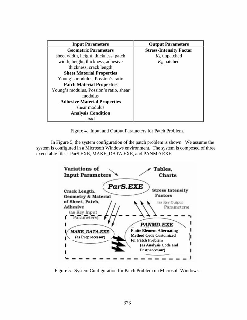
373
Input Parameters Output ParametersGeometric Parameters
sheet width, height, thickness, patchwidth, height, thickness, adhesive
thickness, crack lengthSheet Material Properties
Young’s modulus, Possion’s ratioPatch Material Properties
Young’s modulus, Possion’s ratio, shearmodulus
Adhesive Material Propertiesshear modulus
Analysis Conditionload
Stress-Intensity FactorKI, unpatchedKI, patched
Figure 4. Input and Output Parameters for Patch Problem.
In Figure 5, the system configuration of the patch problem is shown. We assume thesystem is configured in a Microsoft Windows environment. The system is composed of threeexecutable files: ParS.EXE, MAKE_DATA.EXE, and PANMD.EXE.
Figure 5. System Configuration for Patch Problem on Microsoft Windows.
(as Preprocessor)
Finite Element AlternatingMethod Code Customizedfor Patch Problem
(as Analysis Code andPostprocessor)

374
ParS.EXE works as a GUI front end in Microsoft Windows. It controls the analysesfor a parametric survey carried out by MAKE_DATA.EXE and MANMD.EXE whichproduces tables and line charts for visualization of results.
PANMD.EXE is an executable file of the FEAM analysis code customized for thispatch problem. It accepts mesh data, geometry information of a crack, material properties,and analysis conditions for the problem. PANMD.EXE behaves not only as an analysis codebut also as a postprocessor. It then produces stress-intensity factors directly at two end pointsof the crack. ParS.EXE extracts only relevant output parameters from an output filegenerated from PANMD.EXE.
MAKE_DATA.EXE works as a preprocessor for PANMD.EXE. It accepts key inputparameters specified by ParS.EXE and then produces an input file for PANMD.EXE.
All the communications between these processes are carried out by text files. BothMAKE_DATA.EXE and PANMD.EXE must perform without any input from the user,because these routines are executed multiple times automatically by ParS.EXE during aparametric survey.
ParS.EXE is developed as a general purpose parametric survey tool and can beadapted to any other problems. All the dependent knowledge specific to the patch problem isisolated. They are
1. Name of the problem (e.g., Composite patch repairs).
2. Description of each input and output parameter such as a name, unit type, acceptablerange of values, and a default value (e.g., Patch width is the input parameter, unit typeis inches, default value is 3 inches).
3. Names of executable files and text files for analysis code, pre- and postprocessors(e.g., MAKE_DATA, PANMD).
4. Structure of predefined input parameter set databases and each data entry in thedatabases (e.g., Sheet material database where each entry is composed of two inputparameters, Young’s Modulus and Poisson’s ratio).
Figures 6, 7, and 8 show actual screen images of ParS running on Microsoft WindowsNT. In Figure 6, input parameters of patch material property are specified. Each parametervalue can be specified directly through a text field in the dialog box Edit PS in Figure 6 orreferred from the patch material database, as shown in Figure 7.
In Figure 8, the input parameters, the length of the crack, and the type of patchmaterial are changed, and a series of patch analyses are performed. The parameter on the X-axis in the chart is the length of the crack, and the parameter on the Y-axis is the stress-intensity factor (KI) for the patched and unpatched.
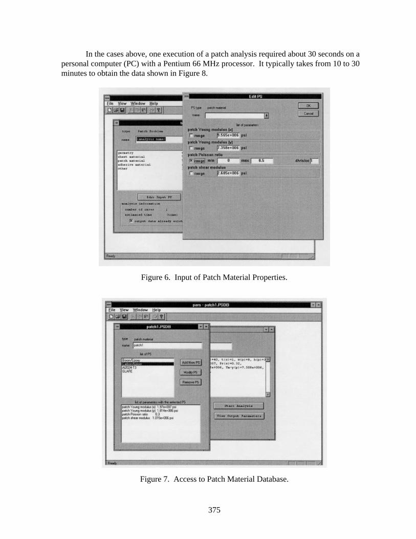
375
In the cases above, one execution of a patch analysis required about 30 seconds on apersonal computer (PC) with a Pentium 66 MHz processor. It typically takes from 10 to 30minutes to obtain the data shown in Figure 8.
Figure 6. Input of Patch Material Properties.
Figure 7. Access to Patch Material Database.
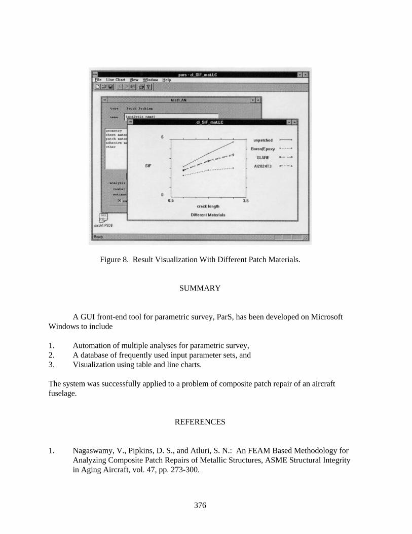
376
Figure 8. Result Visualization With Different Patch Materials.
SUMMARY
A GUI front-end tool for parametric survey, ParS, has been developed on MicrosoftWindows to include
1. Automation of multiple analyses for parametric survey,2. A database of frequently used input parameter sets, and3. Visualization using table and line charts.
The system was successfully applied to a problem of composite patch repair of an aircraftfuselage.
REFERENCES
1. Nagaswamy, V., Pipkins, D. S., and Atluri, S. N.: An FEAM Based Methodology forAnalyzing Composite Patch Repairs of Metallic Structures, ASME Structural Integrityin Aging Aircraft, vol. 47, pp. 273-300.
377
IM PLEMENTATION AND A PPLICATION O F ALARGE-ROTATION FINITE ELEMENT FORMULATION IN
NASA CODE ZIP2DL1
Xiaomin DengDepartment of Mechanical Engineering
University of South CarolinaColumbia, SC
J. C. Newman, Jr.NASA Langley Research Center
Hampton, VA
SUMMARY
Recent stable tearing tests conducted on ARCAN specimens at the NASA LangleyResearch Center indicate that stable crack growth is accompanied by large specimen rotationat the point of loading due to the overall deformation of the specimen. To analyze these testswith proper accounting of the large rotation effects, a total Lagrangian large-deformationfinite element formulation has been implemented in a new NASA crack-growth simulationcode, ZIP2DL, as an extension of the original NASA code, ZIP2D. This new code has beenapplied to a number of crack growth tests on ARCAN specimens using a CTOD fracturecriterion, where the critical CTOD value is determined experimentally. Results so far suggestthat small-deformation simulations underestimate the load predicted by large-deformationsimulations by almost a constant amount, with a relative error of about 6% at the peak load.It appears that by adjusting CTOD within the experimental scatter band, the load againstcrack-growth curve from a large-deformation simulation can be made to agree with test dataover a large range of crack growth, and a major portion of the curve can also be reproducedby a small-deformation simulation with a different CTOD value.
INTRODUCTION
In this paper we discuss the development and application of a new elastic-plasticfinite element code for mixed-mode crack growth simulation under plane stress, plane strain,or mixed state of stress conditions. This new code, named ZIP2DL, is an extension of theexisting NASA code ZIP2D [1, 2], and, in particular, has the ability to handle large-deformation kinematics based on a total Lagrangian finite element formulation. This codehas been successfully applied to simulate stable crack growth experiments conducted on 1 Work done under a grant to the University of South Carolina, NAG-1-1664.
378
ARCAN specimens at the NASA Langley Research Center [3], and to analyze andunderstand the effect of large specimen rotation at the point of loading on crack-growthsimulation under small-deformation conditions, especially on the load against crack growthcurve for both mode I and mixed-mode cases. In the following, we will first outline the finiteelement formulation, then present the results of some verification studies, and finally discussin some detail the findings from our ARCAN test simulations.
FINITE ELEMENT FORMULATION
Consider a body undergoing an arbitrary deformation. Suppose that at the currenttime t the body occupies a domain Ω with boundary Γ (the current configuration) and that atan initial time t0 it occupies a domain Ω0 with boundary Γ0 (the reference configuration).Further, suppose that a material particle is described by its position X at t0 and positionx=x(X, t) at t, and the displacement of the particle at t relative to its position at t0 is u=u(X, t),so that x(X, t)=X+ u(X, t). Following conventions in the literature [3, 4]), we now define ourstress and strain measures. The deformation gradient tensor F is defined by
F x u Fx
X
u
XiJi
JiJ
i
J
= ∇ = + ∇ = = +' '
1 , or ∂∂
δ ∂∂
(1)
where 1 is the second-order identity tensor. The Green-Lagrange strain tensor E is given by
( ) ( ) ( )[ ]E F F u u u uT= ⋅ − = ∇ + ∇ + ∇ ⋅ ∇1
21
1
2
' & & '
(2)
where superscript “T” denotes transposition. Let σ be the (symmetric) Cauchy stress tensor,then the symmetric second Piola-Kirchhoff stress tensor, S, can be defined by
( )S JF FT
= ⋅ ⋅− −1 1σ (3)
where J is the Jacobian and is given by J=detF, which is the determinant of F.
The Principle of Virtual Work at time t+∆t is given by
S t t Ed W t t( ): ( )+ = +∫ ∆ Ω ∆Ω
δ δ0
0
(4)
where on the left-hand side is the internal virtual work stated in the reference configuration;δW is the external virtual work done by external forces (e.g., boundary surface tractions) onδu, and δu and δE are, respectively, the virtual displacement vector and the associatedvirtual strain tensor. It is worth noting that δu and δE are not related to each other by simplyreplacing u and E in Eq. 2 with δu and δE, respectively. Their relationship will be givenlater. To develop an iterative finite element algorithm we express the value of any quantity at
379
time t+∆t as the sum of its value at time t and its increment at time t, so that we can write, forthe stress tensor, displacement vector and strain tensor in the preceding equations,
S t t S S u t t u u E t t E E( ) , ( ) , ( )+ = + + = + + = +∆ ∆ ∆ ∆ ∆ ∆ (5)
where the strain tensor increment ∆E is related to the displacement vector increment ∆u asfollows:
[ ][ ]
∆ ∆ ∆ ∆
∆ ∆ ∆
∆ ∆ ∆
∆ ∆ ∆
E
u u
u u u u
u u
= + +
= ∇ + ∇
= ∇ ⋅ ∇ + ∇ ⋅ ∇
= ∇ ⋅ ∇
ε ε ε
ε
ε
ε
* **
*
**
,
( ) ( ) ,
( ) ( ) ,
( ) ( )
1
21
21
2
' &
& ' & '
& '
(6)
Similarly, the virtual displacement vector and virtual strain tensor can be written as
[ ][ ][ ]
δ δ δ δε δε δε
δε δ δ
δε δ δ
δε δ δ
u u E
u u
u u u u
u u u u
= = + +
= ∇ + ∇
= ∇ ⋅ ∇ + ∇ ⋅ ∇
= ∇ ⋅ ∇ + ∇ ⋅ ∇
∆
∆ ∆
∆ ∆
∆ ∆ ∆ ∆
, ,
( ) ( ) ,
( ) ( ) ,
( ) ( ) ( ) ( )
* **
*
**
1
21
21
2
' &
& ' & '
& ' & '
(7)
Substitution of Eqs. 5-7 into Eq. 4 leads to
[ ] ( )∆ Ω ΩΩ Ω
S E S d W S d: : :** *δ δε δ δε δε+ = − +∫ ∫0 0
0 0
(8)
A generalization of the Hooke’s law to arbitrarily large deformation cases is given by
S C E S C E= =: : or ∆ ∆ (9)
where C is the conventional fourth-order elasticity tensor. To apply the theory of plasticity,we note that, when measured in the reference configuration Ω0, the tensors E and S areinvariant under arbitrary rigid-body rotations. As such, they can be used in place of theengineering strain and stress measures in small-strain constitutive equations under generallarge-rotation and small-strain deformation conditions. For example, a generalization of anincremental theory of plasticity (e.g., the J2 flow theory of plasticity used in the current study)to large-deformation (rotation) but small-strain cases can be written as
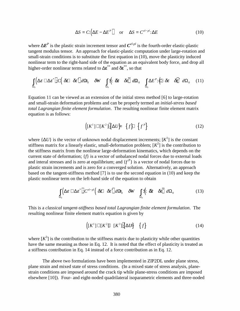
380
( )∆ ∆ ∆ ∆ ∆S C E E S C EP el pl= − = −: : or (10)
where ∆EP is the plastic strain increment tensor and Cel-pl is the fourth-order elastic-plastictangent modulus tensor. An approach for elastic-plastic computation under large-rotation andsmall-strain conditions is to substitute the first equation in (10), move the plasticity inducednonlinear term to the right-hand side of the equation as an equivalent body force, and drop allhigher-order nonlinear terms related to ∆εε** and δεε** , so that
( ) ( ) ( ) ( )∆ ∆ Ω Ω ∆ ΩΩ Ω Ω
ε ε δε δε δ δε δε δε δε+ + = − + + +∫ ∫ ∫* * * *: : : : :C d W S d E C dP0 0 0
0 0 0
(11)
Equation 11 can be viewed as an extension of the initial stress method [6] to large-rotationand small-strain deformation problems and can be properly termed an initial-stress basedtotal Lagrangian finite element formulation. The resulting nonlinear finite element matrixequation is as follows:
( ) [ ] [ ]K K U f f P1 2+ = +∆ (12)
where ∆U is the vector of unknown nodal displacement increments; [K1] is the constantstiffness matrix for a linearly elastic, small-deformation problem; [K2] is the contribution tothe stiffness matrix from the nonlinear large-deformation kinematics, which depends on thecurrent state of deformation; f is a vector of unbalanced nodal forces due to external loadsand interal stresses and is zero at equilibrium; and f P is a vector of nodal forces due toplastic strain increments and is zero for a converged solution. Alternatively, an approachbased on the tangent-stiffness method [7] is to use the second equation in (10) and keep theplastic nonlinear term on the left-hand side of the equation to obtain
( ) ( ) ( )∆ ∆ Ω ΩΩ Ω
ε ε δε δε δ δε δε+ + = − +−∫ ∫* * *: : :C d W S del pl0 0
0 0
(13)
This is a classical tangent-stiffness based total Lagrangian finite element formulation. Theresulting nonlinear finite element matrix equation is given by
( ) [ ] [ ] [ ]K K K U f1 2 3+ + =∆ (14)
where [K3] is the contribution to the stiffness matrix due to plasticity while other quantitieshave the same meaning as those in Eq. 12. It is noted that the effect of plasticity is treated asa stiffness contribution in Eq. 14 instead of a force contribution as in Eq. 12.
The above two formulations have been implemented in ZIP2DL under plane stress,plane strain and mixed state of stress conditions. (In a mixed state of stress analysis, plane-strain conditions are imposed around the crack tip while plane-stress conditions are imposedelsewhere [10]). Four- and eight-noded quadrilateral isoparametric elements and three-noded
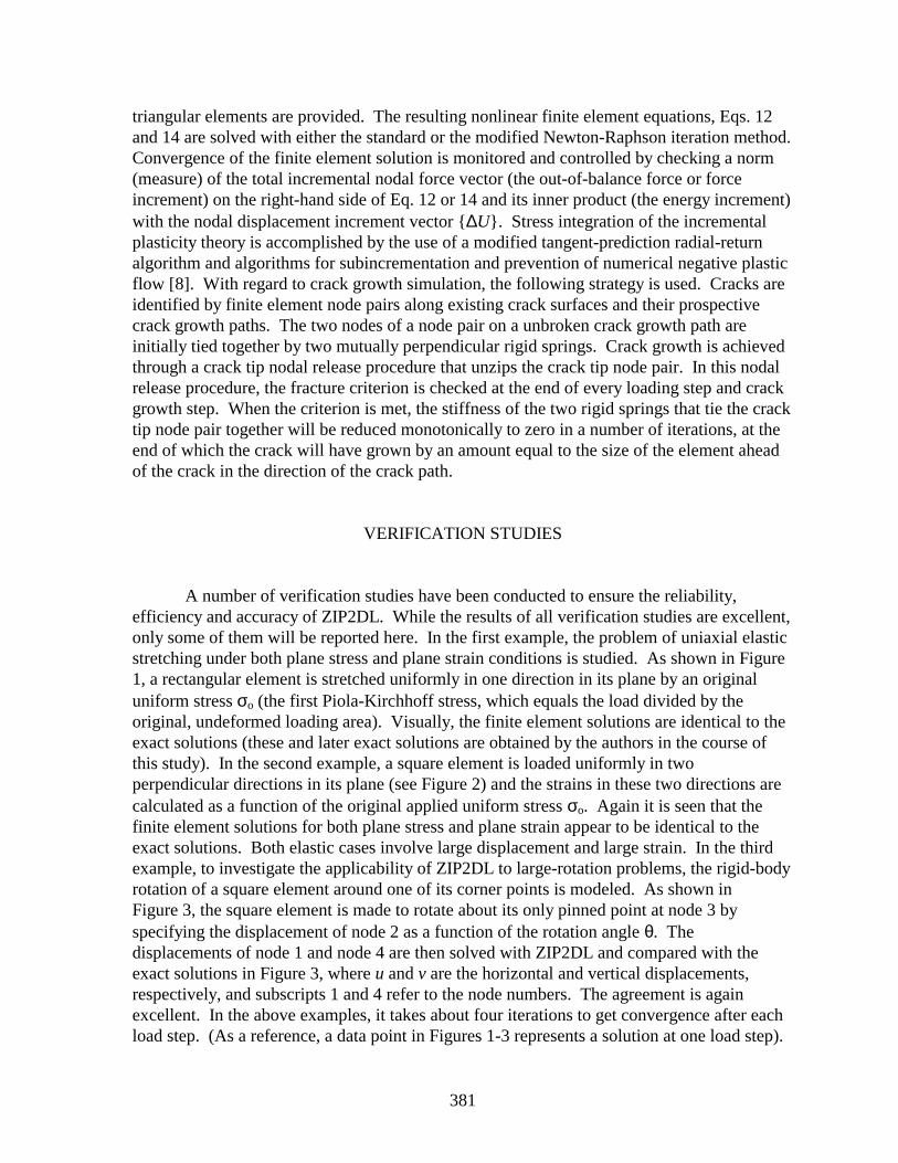
381
triangular elements are provided. The resulting nonlinear finite element equations, Eqs. 12and 14 are solved with either the standard or the modified Newton-Raphson iteration method.Convergence of the finite element solution is monitored and controlled by checking a norm(measure) of the total incremental nodal force vector (the out-of-balance force or forceincrement) on the right-hand side of Eq. 12 or 14 and its inner product (the energy increment)with the nodal displacement increment vector ∆U. Stress integration of the incrementalplasticity theory is accomplished by the use of a modified tangent-prediction radial-returnalgorithm and algorithms for subincrementation and prevention of numerical negative plasticflow [8]. With regard to crack growth simulation, the following strategy is used. Cracks areidentified by finite element node pairs along existing crack surfaces and their prospectivecrack growth paths. The two nodes of a node pair on a unbroken crack growth path areinitially tied together by two mutually perpendicular rigid springs. Crack growth is achievedthrough a crack tip nodal release procedure that unzips the crack tip node pair. In this nodalrelease procedure, the fracture criterion is checked at the end of every loading step and crackgrowth step. When the criterion is met, the stiffness of the two rigid springs that tie the cracktip node pair together will be reduced monotonically to zero in a number of iterations, at theend of which the crack will have grown by an amount equal to the size of the element aheadof the crack in the direction of the crack path.
VERIFICATION STUDIES
A number of verification studies have been conducted to ensure the reliability,efficiency and accuracy of ZIP2DL. While the results of all verification studies are excellent,only some of them will be reported here. In the first example, the problem of uniaxial elasticstretching under both plane stress and plane strain conditions is studied. As shown in Figure1, a rectangular element is stretched uniformly in one direction in its plane by an originaluniform stress σo (the first Piola-Kirchhoff stress, which equals the load divided by theoriginal, undeformed loading area). Visually, the finite element solutions are identical to theexact solutions (these and later exact solutions are obtained by the authors in the course ofthis study). In the second example, a square element is loaded uniformly in twoperpendicular directions in its plane (see Figure 2) and the strains in these two directions arecalculated as a function of the original applied uniform stress σo. Again it is seen that thefinite element solutions for both plane stress and plane strain appear to be identical to theexact solutions. Both elastic cases involve large displacement and large strain. In the thirdexample, to investigate the applicability of ZIP2DL to large-rotation problems, the rigid-bodyrotation of a square element around one of its corner points is modeled. As shown inFigure 3, the square element is made to rotate about its only pinned point at node 3 byspecifying the displacement of node 2 as a function of the rotation angle θ. Thedisplacements of node 1 and node 4 are then solved with ZIP2DL and compared with theexact solutions in Figure 3, where u and v are the horizontal and vertical displacements,respectively, and subscripts 1 and 4 refer to the node numbers. The agreement is againexcellent. In the above examples, it takes about four iterations to get convergence after eachload step. (As a reference, a data point in Figures 1-3 represents a solution at one load step).
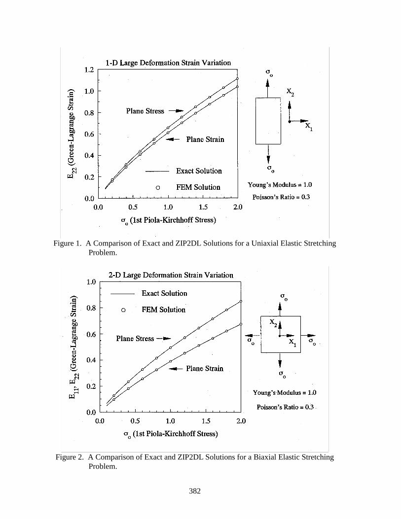
382
Figure 1. A Comparison of Exact and ZIP2DL Solutions for a Uniaxial Elastic StretchingProblem.
Figure 2. A Comparison of Exact and ZIP2DL Solutions for a Biaxial Elastic StretchingProblem.
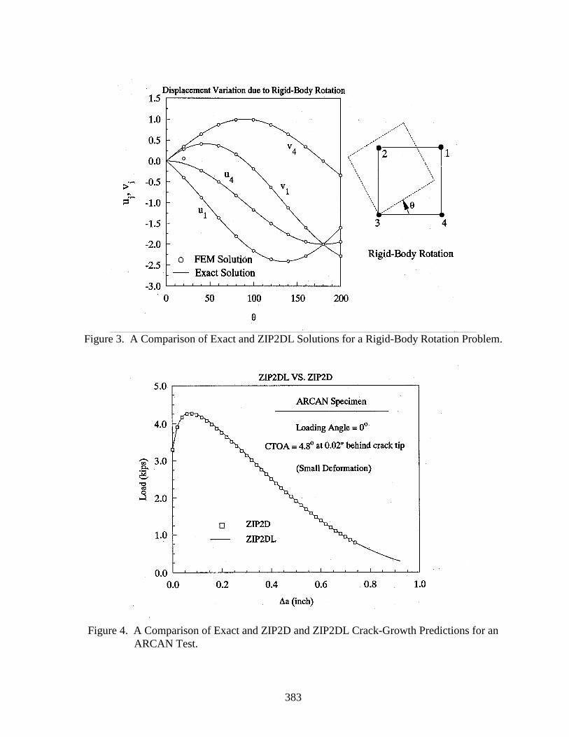
383
Figure 3. A Comparison of Exact and ZIP2DL Solutions for a Rigid-Body Rotation Problem.
Figure 4. A Comparison of Exact and ZIP2D and ZIP2DL Crack-Growth Predictions for anARCAN Test.
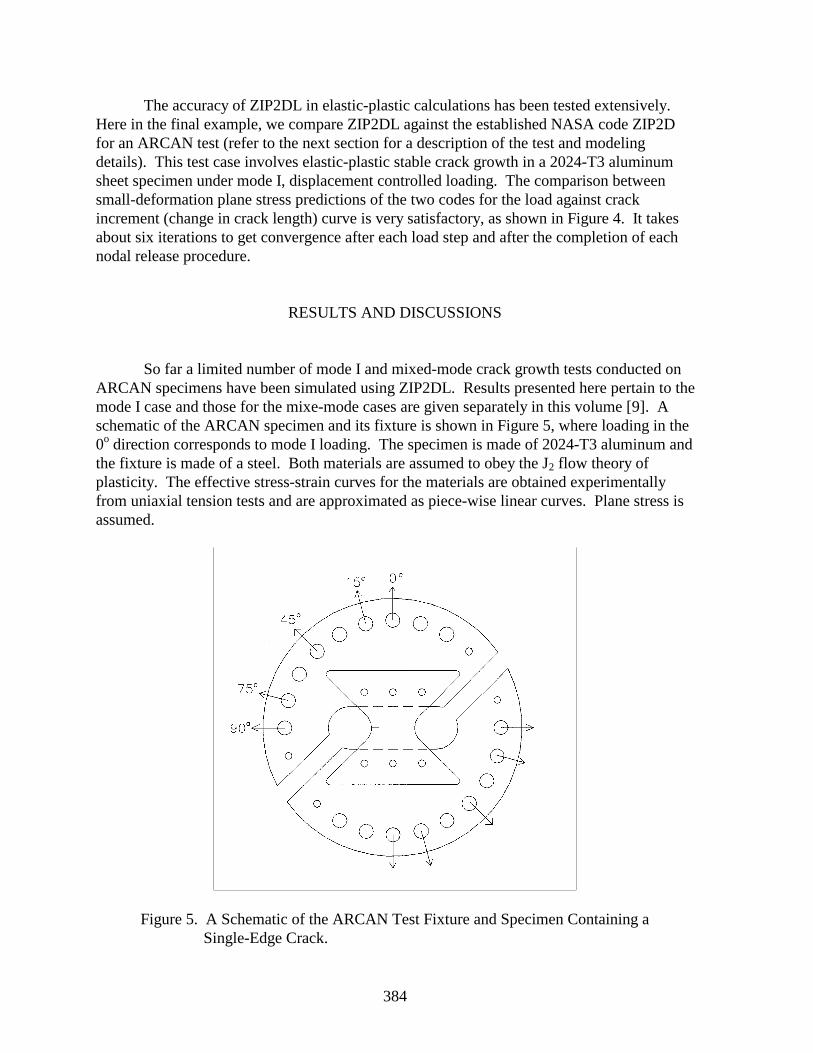
384
The accuracy of ZIP2DL in elastic-plastic calculations has been tested extensively.Here in the final example, we compare ZIP2DL against the established NASA code ZIP2Dfor an ARCAN test (refer to the next section for a description of the test and modelingdetails). This test case involves elastic-plastic stable crack growth in a 2024-T3 aluminumsheet specimen under mode I, displacement controlled loading. The comparison betweensmall-deformation plane stress predictions of the two codes for the load against crackincrement (change in crack length) curve is very satisfactory, as shown in Figure 4. It takesabout six iterations to get convergence after each load step and after the completion of eachnodal release procedure.
RESULTS AND DISCUSSIONS
So far a limited number of mode I and mixed-mode crack growth tests conducted onARCAN specimens have been simulated using ZIP2DL. Results presented here pertain to themode I case and those for the mixe-mode cases are given separately in this volume [9]. Aschematic of the ARCAN specimen and its fixture is shown in Figure 5, where loading in the0o direction corresponds to mode I loading. The specimen is made of 2024-T3 aluminum andthe fixture is made of a steel. Both materials are assumed to obey the J2 flow theory ofplasticity. The effective stress-strain curves for the materials are obtained experimentallyfrom uniaxial tension tests and are approximated as piece-wise linear curves. Plane stress isassumed.
Figure 5. A Schematic of the ARCAN Test Fixture and Specimen Containing aSingle-Edge Crack.
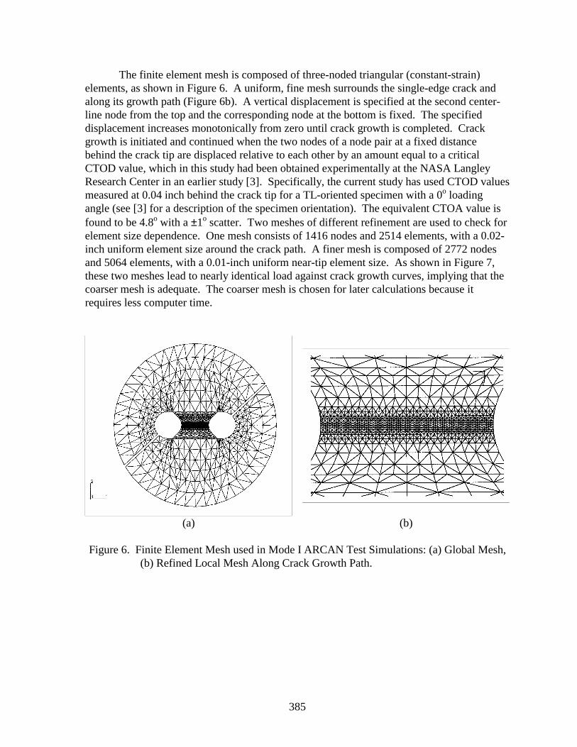
385
The finite element mesh is composed of three-noded triangular (constant-strain)elements, as shown in Figure 6. A uniform, fine mesh surrounds the single-edge crack andalong its growth path (Figure 6b). A vertical displacement is specified at the second center-line node from the top and the corresponding node at the bottom is fixed. The specifieddisplacement increases monotonically from zero until crack growth is completed. Crackgrowth is initiated and continued when the two nodes of a node pair at a fixed distancebehind the crack tip are displaced relative to each other by an amount equal to a criticalCTOD value, which in this study had been obtained experimentally at the NASA LangleyResearch Center in an earlier study [3]. Specifically, the current study has used CTOD valuesmeasured at 0.04 inch behind the crack tip for a TL-oriented specimen with a 0o loadingangle (see [3] for a description of the specimen orientation). The equivalent CTOA value isfound to be 4.8o with a ±1o scatter. Two meshes of different refinement are used to check forelement size dependence. One mesh consists of 1416 nodes and 2514 elements, with a 0.02-inch uniform element size around the crack path. A finer mesh is composed of 2772 nodesand 5064 elements, with a 0.01-inch uniform near-tip element size. As shown in Figure 7,these two meshes lead to nearly identical load against crack growth curves, implying that thecoarser mesh is adequate. The coarser mesh is chosen for later calculations because itrequires less computer time.
(a) (b)
Figure 6. Finite Element Mesh used in Mode I ARCAN Test Simulations: (a) Global Mesh,(b) Refined Local Mesh Along Crack Growth Path.
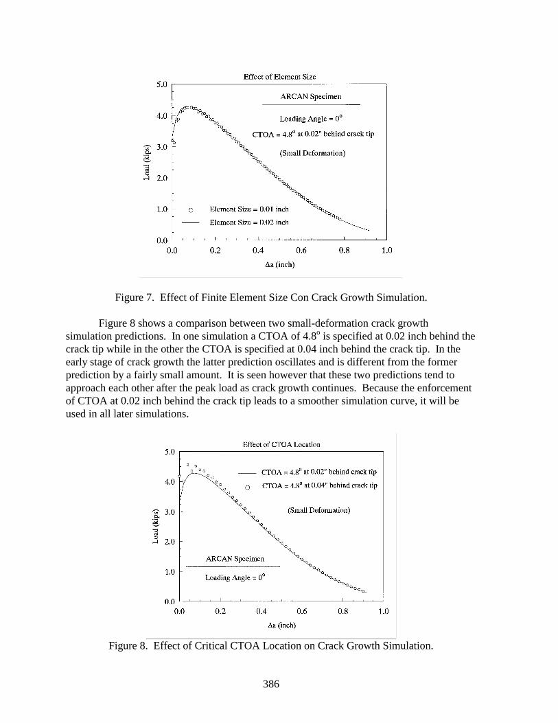
386
Figure 7. Effect of Finite Element Size Con Crack Growth Simulation.
Figure 8 shows a comparison between two small-deformation crack growthsimulation predictions. In one simulation a CTOA of 4.8o is specified at 0.02 inch behind thecrack tip while in the other the CTOA is specified at 0.04 inch behind the crack tip. In theearly stage of crack growth the latter prediction oscillates and is different from the formerprediction by a fairly small amount. It is seen however that these two predictions tend toapproach each other after the peak load as crack growth continues. Because the enforcementof CTOA at 0.02 inch behind the crack tip leads to a smoother simulation curve, it will beused in all later simulations.
Figure 8. Effect of Critical CTOA Location on Crack Growth Simulation.
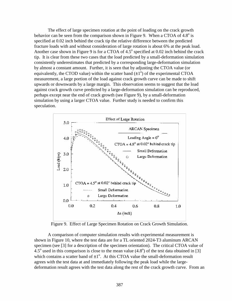
387
The effect of large specimen rotation at the point of loading on the crack growthbehavior can be seen from the comparison shown in Figure 9. When a CTOA of 4.8o isspecified at 0.02 inch behind the crack tip the relative difference between the predictedfracture loads with and without consideration of large rotation is about 6% at the peak load.Another case shown in Figure 9 is for a CTOA of 4.5o specified at 0.02 inch behind the cracktip. It is clear from these two cases that the load predicted by a small-deformation simulationconsistently underestimates that predicted by a corresponding large-deformation simulationby almost a constant amount. Further, it is seen that by adjusting the CTOA value (orequivalently, the CTOD value) within the scatter band (±1o) of the experimental CTOAmeasurement, a large portion of the load against crack growth curve can be made to shiftupwards or downwards by a large margin. This observation seems to suggest that the loadagainst crack growth curve predicted by a large-deformation simulation can be reproduced,perhaps except near the end of crack growth (see Figure 9), by a small-deformationsimulation by using a larger CTOA value. Further study is needed to confirm thisspeculation.
Figure 9. Effect of Large Specimen Rotation on Crack Growth Simulation.
A comparison of computer simulation results with experimental measurement isshown in Figure 10, where the test data are for a TL oriented 2024-T3 aluminum ARCANspecimen (see [3] for a description of the specimen orientation). The critical CTOA value of4.5o used in this comparison is close to the mean value (4.8o) of the test data obtained in [3]which contains a scatter band of ±1o. At this CTOA value the small-deformation resultagrees with the test data at and immediately following the peak load while the large-deformation result agrees with the test data along the rest of the crack growth curve. From an
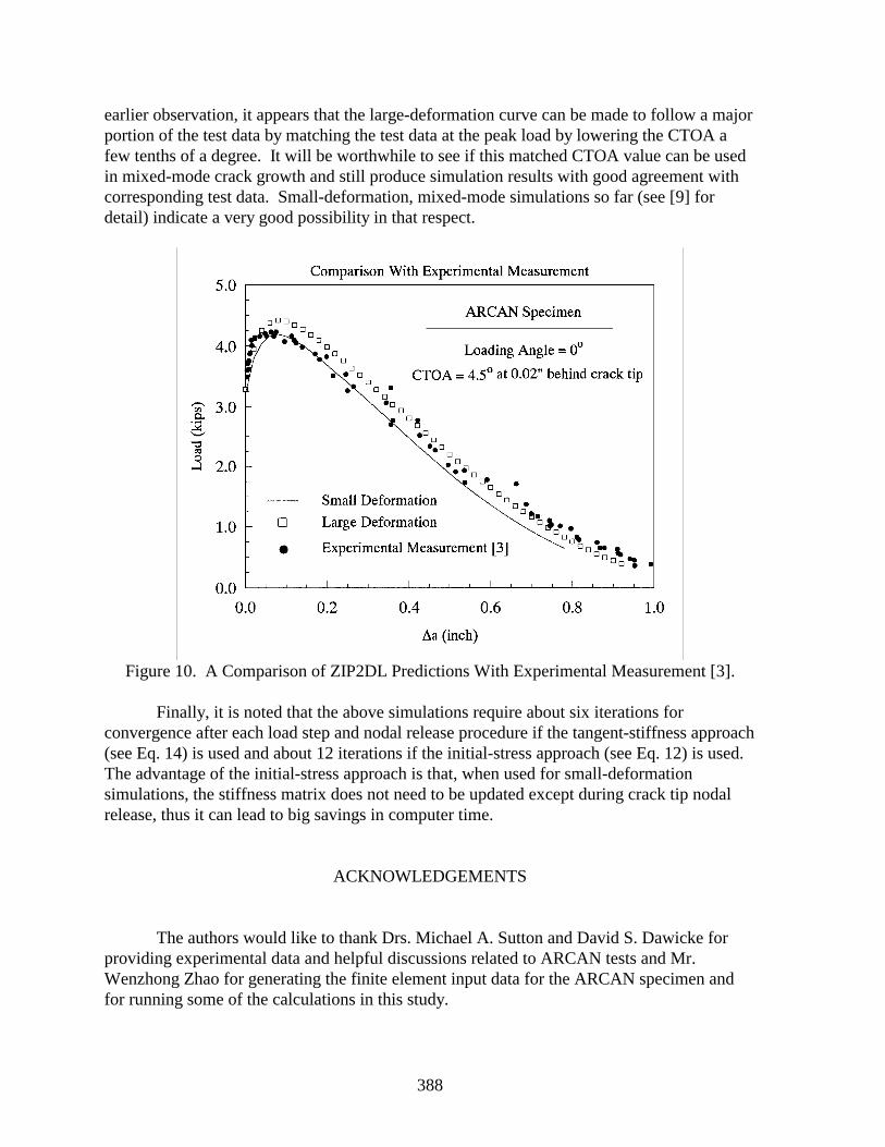
388
earlier observation, it appears that the large-deformation curve can be made to follow a majorportion of the test data by matching the test data at the peak load by lowering the CTOA afew tenths of a degree. It will be worthwhile to see if this matched CTOA value can be usedin mixed-mode crack growth and still produce simulation results with good agreement withcorresponding test data. Small-deformation, mixed-mode simulations so far (see [9] fordetail) indicate a very good possibility in that respect.
Figure 10. A Comparison of ZIP2DL Predictions With Experimental Measurement [3].
Finally, it is noted that the above simulations require about six iterations forconvergence after each load step and nodal release procedure if the tangent-stiffness approach(see Eq. 14) is used and about 12 iterations if the initial-stress approach (see Eq. 12) is used.The advantage of the initial-stress approach is that, when used for small-deformationsimulations, the stiffness matrix does not need to be updated except during crack tip nodalrelease, thus it can lead to big savings in computer time.
ACKNOWLEDGEMENTS
The authors would like to thank Drs. Michael A. Sutton and David S. Dawicke forproviding experimental data and helpful discussions related to ARCAN tests and Mr.Wenzhong Zhao for generating the finite element input data for the ARCAN specimen andfor running some of the calculations in this study.
389/390
REFERENCES
1. Newman, J.C., Jr.: Finite-Element Analysis of Fatigue Crack Propagation Includingthe Effects of Crack Closure. Ph.D. Thesis, Virginia Polytechnic Institute,Blacksburg, VA, 1974.
2. Newman, J.C., Jr.: User guide for ZIP2D. NASA Langley Research Center,Hampton, Virginia, modified April 2, 1996.
3. Amstutz, B.E.; Sutton, M.A.; Dawicke, D.S.; and Boone, M.L.: Effects of Mixed-Mode I/II Loading and Grain Orientation on Crack Initiation and Stable Tearing in2024-T3 Aluminum. Fatigue and Fracture Mechanics: 27th Volume, ASTM STP1296, R. S. Piascik, J.C. Newman, Jr., and N.E. Dowling, Eds, American Society forTesting and Materials, Philadephia, 1995.
4. Malvern, L.E.: Introduction to the Mechanics of a Continuous Medium. Prentice-Hall, Englewood Cliffs, New Jersey, 1969.
5. Bathe, K.-J.: Finite Element Procedures. Prentice-Hall, Englewood Cliffs, NewJersey, 1996.
6. Zienkiewicz, O.C.; Valliappan, S.; and King, I.P.: Elasto-Plastic Solutions ofEngineering Problems: Initial Stress Finite Element Approach. International Journalfor Numerical Methods in Engineering, Vol. 1, 1969, pp. 75-100.
7. Marcal, P.V.: A Stiffness Method for Elastic-Plastic Problems. Int. J. Mech. Sci.,Vol. 7, 1965, pp. 220-238.
8. Deng, X.; and Rosakis, A.J.: Negative Plastic Flow and its Prevention in Elasto-Plastic Finite Element Computation. Finite Element in Analysis and Design, Vol. 7,1990, 181-191.
9. Sutton, M.A.; Zhao, W.; Dawicke, D.S.; Deng, X.; and Newman, J.C., Jr.: NumericalInvestigations into the Viability of CTOD as a Fracture Parameter for Mixed-ModeI/II Tearing of Thin Aluminum Sheets. FAA-NASA Symposium on ContinuedAirworthiness of Aircraft Structures, 1996.
10. Newman, J.C.; Booth, B.C.; and Shivakumar, K.N.: An Elastic-Plastic Einite-Element Analysis of the J-Resistance Curve Using a CTOD Criterion. FractureMechanics: Eighteenth Symposium, ASTM STP 945, D. T. Read and R. P. Reed,Eds., American Society for Testing and Materials, Philadephia, 1988.
391
IM PLICATIONS O F CORROSION PILLOWING ON THESTRUCTURAL INTEGRITY O F FUSELAGE LA P JOINTS*
Nicholas C. Bellinger and Jerzy P. KomorowskiStructures, Materials, and Propulsion Laboratory
Institute for Aerospace ResearchNational Research Council Canada
Ottawa, Ontario, Canada
SUMMARY
Finite element techniques were used to determine the effect that pillowing, caused bythe presence of corrosion products, has on fuselage lap joints. The stress caused by theinternal pressure and riveting process was taken into account while the fuselage curvaturewas ignored. The results indicate that as the pillowing (i.e. thickness loss) increases, thestress in the joint increases. Also, these results suggest that the volume of corrosion productspresent within a joint is the main parameter governing the increase in stress and not thepercent thickness loss. For example, if a joint contains 5% thickness loss in each skin,although the total thickness loss is only 5%, the volume of corrosion products is equivalent toa 10% thickness loss in one skin. A preliminary fracture mechanics analysis carried out on asingle crack located just beyond the rivet head suggests that the crack edge along the fayingsurface would grow more rapidly along the rivet row forming a semielliptical crack front witha very high aspect ratio. This type of crack is more difficult to detect during visualinspection.
INTRODUCTION
Concern has grown as to the possible effects corrosion might have on the structuralintegrity of fuselage lap joints. Environmental attack can lead to early crack initiation,enhanced crack growth rates (corrosion fatigue), thickness loss (increased stresses), andintergranular and stress corrosion cracking and pitting (stress risers). Present maintenanceguidelines allow for a maximum thickness loss of 10% within a single skin before repairsmust be made to a joint (ref. 1). However, in a previous study carried out at the NationalResearch Council Canada (NRCC), the volumetric increase associated with corrosion by-products was found to be approximately 6.5 times greater than the volume of parent materiallost (ref. 2). This large volumetric increase results in local deformations (pillowing) whichcan affect the structural integrity of fuselage lap joints.
* Work carried out under collaborative research agreement between National Research Council and DiffractoLimited dated June 1995. Project funded by the U.S. Air Force through the Federal Aviation Administrationand by Transport Canada, NRC, and Diffracto Limited.
392
Finite element techniques along with a mathematical model (ref. 3) were used tosimulate the presence of corrosion products within a fuselage lap joint. The stress resultingfrom the internal pressure (hoop stress), the prestress caused by the rivet fastening processand the reduction in thickness caused by the material loss were all taken into account whilethe curvature of the fuselage was ignored. The results indicated that the stress in the area ofthe rivets increases significantly due to the presence of corrosion pillowing. A fracturemechanics analysis was also carried out on a single crack of a length just beyond the rivethead to help assess the structural integrity implications of corrosion pillowing.
FINITE ELEMENT MODEL
A typical lap joint configuration was chosen for this study and consisted of two skins(outer and inner) of equal thickness, 1.14 mm (0.045 in), fabricated from Al 2024-T3. Theskins were joined using three rows of rivets with a 25.4 mm (1.0 inch) spacing. Each rivethad a nominal shank diameter of 3.96 mm (0.156 inch) and a rivet head diameter of 5.8 mm(0.232 inch). A hat-section stringer was attached to the middle rivet row through the hatcrown as shown in Figure 1. Three finite element models were generated to simulate thedifferent loads that are present within a corroded joint. These loads were; 1) hoop stresscaused by the internal pressure, 2) prestress caused by the riveting process and, 3) stress dueto corrosion pillowing. To save computation time and storage space only three rivets weremodeled as shown in Figure 2. The rivet/skin interaction was simulated using nonlinear gapelements.
Stress Analysis
All models were generated using the first-order brick elements available in the NISAfinite element package. It was assumed for the hoop stress model that some of the loadtransfer would be due to friction under the rivet heads which was simulated by merging thenodes in these areas. A pressure was applied along a skin edge to simulate the hoop stresswhile the opposing edge was fixed in all directions. For the prestress model, all the nodeswere merged to prevent the skins from penetrating, and a pressure was applied to the rivetheads to simulate the riveting process. To model the corrosion pillowing, a three-stageprocess was used; 1) a 6.89 kPa (1 psi) pressure was initially applied to the faying surfacesand the resulting volume determined, 2) given a specified thickness loss in one skin, thevolume required to accommodate the corrosion products was calculated using a previouslyderived formula (ref. 3-4), and 3) assuming a linear relationship between the applied pressureand volume due to the incompressibility of the corrosion products, the pressure necessary toobtain the required volume was calculated and then reapplied to the faying surfaces (ref. 4).The finite element analysis was then rerun and the resulting displacements obtained.
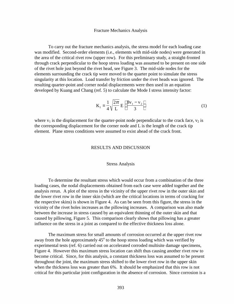
393
Fracture Mechanics Analysis
To carry out the fracture mechanics analysis, the stress model for each loading casewas modified. Second-order elements (i.e., elements with mid-side nodes) were generated inthe area of the critical rivet row (upper row). For this preliminary study, a straight-frontedthrough crack perpendicular to the hoop stress loading was assumed to be present on one sideof the rivet hole just beyond the rivet head, see Figure 3. The mid-side nodes for theelements surrounding the crack tip were moved to the quarter point to simulate the stresssingularity at this location. Load transfer by friction under the rivet heads was ignored. Theresulting quarter-point and corner nodal displacements were then used in an equationdeveloped by Kuang and Chang (ref. 5) to calculate the Mode I stress intensity factor:
K1
4
2
L E
8v v
3I1 2=
−
π(1)
where v1 is the displacement for the quarter-point node perpendicular to the crack face, v2 isthe corresponding displacement for the corner node and L is the length of the crack tipelement. Plane stress conditions were assumed to exist ahead of the crack front.
RESULTS AND DISCUSSION
Stress Analysis
To determine the resultant stress which would occur from a combination of the threeloading cases, the nodal displacements obtained from each case were added together and theanalysis rerun. A plot of the stress in the vicinity of the upper rivet row in the outer skin andthe lower rivet row in the inner skin (which are the critical locations in terms of cracking forthe respective skins) is shown in Figure 4. As can be seen from this figure, the stress in thevicinity of the rivet holes increases as the pillowing increases. A comparison was also madebetween the increase in stress caused by an equivalent thinning of the outer skin and thatcaused by pillowing, Figure 5. This comparison clearly shows that pillowing has a greaterinfluence on the stress in a joint as compared to the effective thickness loss alone.
The maximum stress for small amounts of corrosion occurred at the upper rivet rowaway from the hole approximately 45o to the hoop stress loading which was verified byexperimental tests (ref. 6) carried out on accelerated corroded multisite damage specimens,Figure 4. However this maximum stress location can shift thus causing another rivet row tobecome critical. Since, for this analysis, a constant thickness loss was assumed to be presentthroughout the joint, the maximum stress shifted to the lower rivet row in the upper skinwhen the thickness loss was greater than 6%. It should be emphasized that this row is notcritical for this particular joint configuration in the absence of corrosion. Since corrosion is a
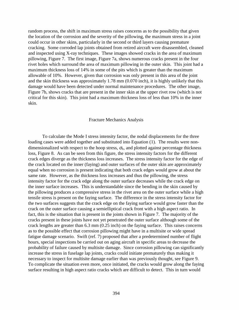
394
random process, the shift in maximum stress raises concerns as to the possibility that giventhe location of the corrosion and the severity of the pillowing, the maximum stress in a jointcould occur in other skins, particularly in the second or third layers causing prematurecracking. Some corroded lap joints obtained from retired aircraft were disassembled, cleanedand inspected using X-ray techniques. These images showed cracks in the area of maximumpillowing, Figure 7. The first image, Figure 7a, shows numerous cracks present in the fourrivet holes which surround the area of maximum pillowing in the outer skin. This joint had amaximum thickness loss of 14% in some of the pits which is greater than the maximumallowable of 10%. However, given that corrosion was only present in this area of the jointand the skin thickness was approximately 1.78 mm (0.070 inch), it is highly unlikely that thisdamage would have been detected under normal maintenance procedures. The other image,Figure 7b, shows cracks that are present in the inner skin at the upper rivet row (which is notcritical for this skin). This joint had a maximum thickness loss of less than 10% in the innerskin.
Fracture Mechanics Analysis
To calculate the Mode I stress intensity factor, the nodal displacements for the threeloading cases were added together and substituted into Equation (1). The results were non-dimensionalized with respect to the hoop stress, σh, and plotted against percentage thicknessloss, Figure 8. As can be seen from this figure, the stress intensity factors for the differentcrack edges diverge as the thickness loss increases. The stress intensity factor for the edge ofthe crack located on the inner (faying) and outer surfaces of the outer skin are approximatelyequal when no corrosion is present indicating that both crack edges would grow at about thesame rate. However, as the thickness loss increases and thus the pillowing, the stressintensity factor for the crack edge along the outer surface decreases while the crack edge onthe inner surface increases. This is understandable since the bending in the skin caused bythe pillowing produces a compressive stress in the rivet area on the outer surface while a hightensile stress is present on the faying surface. The difference in the stress intensity factor forthe two surfaces suggests that the crack edge on the faying surface would grow faster than thecrack on the outer surface causing a semielliptical crack front with a high aspect ratio. Infact, this is the situation that is present in the joints shown in Figure 7. The majority of thecracks present in these joints have not yet penetrated the outer surface although some of thecrack lengths are greater than 6.3 mm (0.25 inch) on the faying surface. This raises concernsas to the possible effect that corrosion pillowing might have in a multisite or wide spreadfatigue damage scenario. Swift (ref. 7) proposed that after a predetermined number of flighthours, special inspections be carried out on aging aircraft in specific areas to decrease theprobability of failure caused by multisite damage. Since corrosion pillowing can significantlyincrease the stress in fuselage lap joints, cracks could initiate prematurely thus making itnecessary to inspect for multisite damage earlier than was previously thought, see Figure 9.To complicate the situation even more, once initiated, the cracks would grow along the fayingsurface resulting in high aspect ratio cracks which are difficult to detect. This in turn would
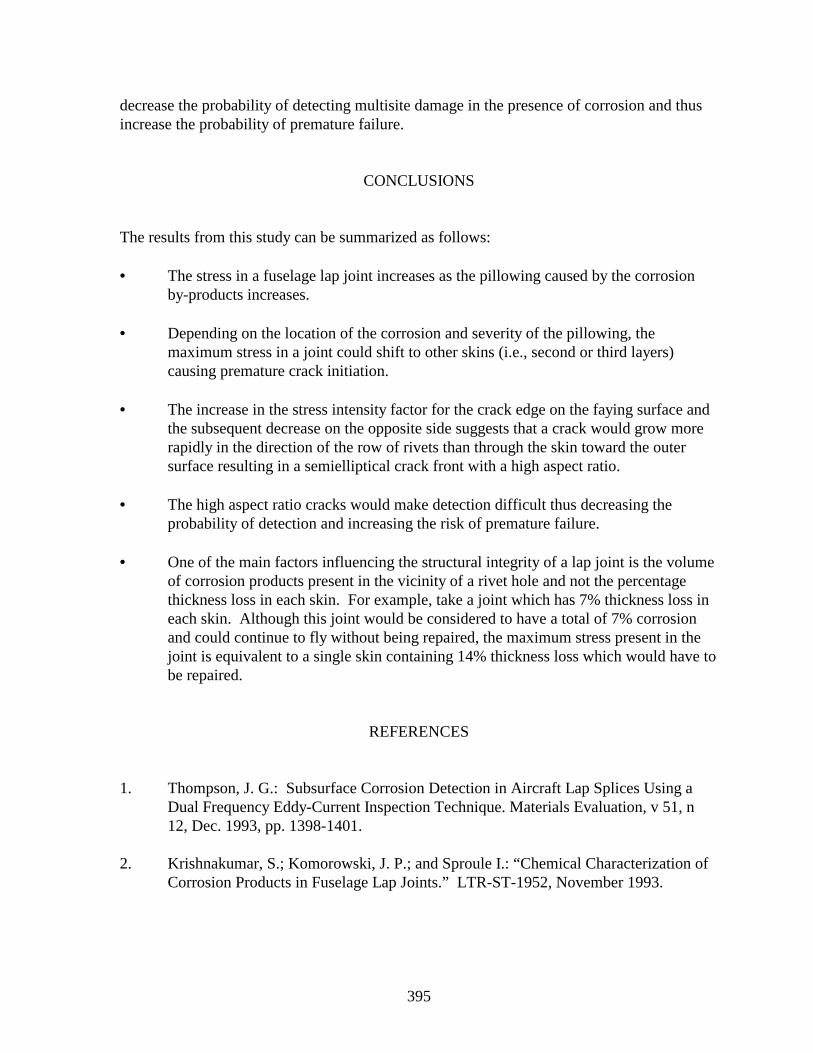
395
decrease the probability of detecting multisite damage in the presence of corrosion and thusincrease the probability of premature failure.
CONCLUSIONS
The results from this study can be summarized as follows:
• The stress in a fuselage lap joint increases as the pillowing caused by the corrosionby-products increases.
• Depending on the location of the corrosion and severity of the pillowing, themaximum stress in a joint could shift to other skins (i.e., second or third layers)causing premature crack initiation.
• The increase in the stress intensity factor for the crack edge on the faying surface andthe subsequent decrease on the opposite side suggests that a crack would grow morerapidly in the direction of the row of rivets than through the skin toward the outersurface resulting in a semielliptical crack front with a high aspect ratio.
• The high aspect ratio cracks would make detection difficult thus decreasing theprobability of detection and increasing the risk of premature failure.
• One of the main factors influencing the structural integrity of a lap joint is the volumeof corrosion products present in the vicinity of a rivet hole and not the percentagethickness loss in each skin. For example, take a joint which has 7% thickness loss ineach skin. Although this joint would be considered to have a total of 7% corrosionand could continue to fly without being repaired, the maximum stress present in thejoint is equivalent to a single skin containing 14% thickness loss which would have tobe repaired.
REFERENCES
1. Thompson, J. G.: Subsurface Corrosion Detection in Aircraft Lap Splices Using aDual Frequency Eddy-Current Inspection Technique. Materials Evaluation, v 51, n12, Dec. 1993, pp. 1398-1401.
2. Krishnakumar, S.; Komorowski, J. P.; and Sproule I.: “Chemical Characterization of
Corrosion Products in Fuselage Lap Joints.” LTR-ST-1952, November 1993.

396
3. Bellinger, N. C.; Krishnakumar, S.; and Komorowski, J. P.: Modelling of PillowingDue to Corrosion in Fuselage Lap Joints. CAS Journal, Vol. 40, No. 3, September1994, pp. 125-130.
4. Bellinger, N. C.; Komorowski, J. P.; and Krishnakumar, S.: Numerical Modelling of
Pillowing Due to Corrosion in Fuselage Lap Joints. LTR-ST-2005, April 1995. 5. Beres, W.: NSIFS Postprocessor for Displacement-Based Stress Intensity Factor
Extraction from NISA II Calculation Results. ST-727, October 17, 1994. 6. Wakeman, R. B.: Interaction of Multiple Site Fatigue Damage and Corrosion in
Fuselage Lap Splices. Master’s Thesis, Carleton University, Ottawa, Canada, to bepublished.
7. Swift, T.: Widespread Fatigue Damage Monitoring - Issues and Concerns. NASA
CP 3274, FAA/NASA International Symposium on Advanced Structural IntegrityMethods for Airframe Durability and Damage Tolerance, Sept. 1994, pp. 829-870.
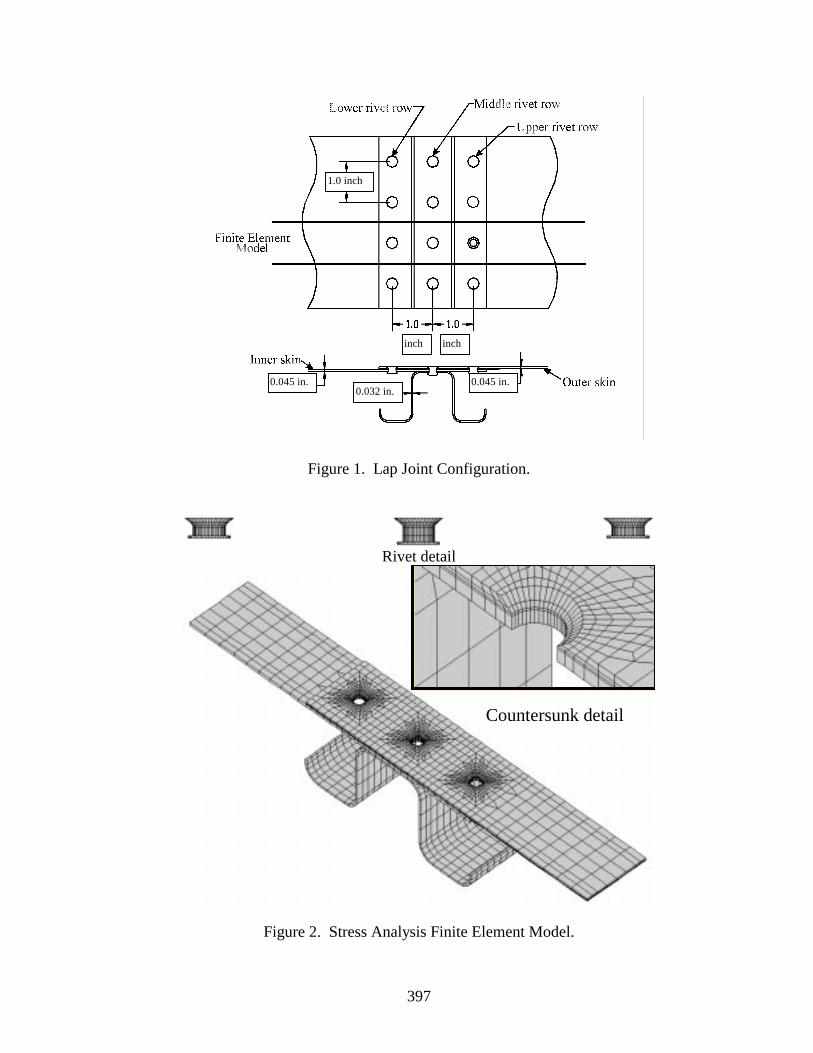
397
Figure 1. Lap Joint Configuration.
Rivet detail
Countersunk detail
Figure 2. Stress Analysis Finite Element Model.
1.0 inch
inch inch
0.045 in. 0.045 in.0.032 in.

398
Crack
Crack
Inner skin
Outer skin
(a) Critical Rivet Row Detail (b) Boundary Line Plot Showing Crack.
Figure 3. Fracture Mechanics Finite Element Model.
0 1 2 3 4 5 6 7 8 9 10 11 12 13
% Thickness Loss
0
1
2
3
4
5
6
7
8
σ 1, m
ax /
σ1,
re
mot
e
Yield Strength
2024-T3
Outer SkinInner Skin
Figure 4. Effect of Increased Corrosion Pillowing on Critical Rivet Row of RespectiveSkins.
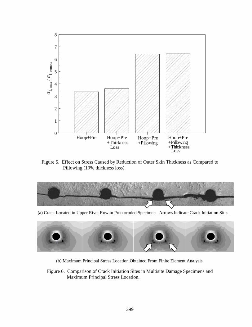
399
0
1
2
3
4
5
6
7
8
σ 1, m
ax /
σ 1, r
emot
e
Hoop+Pre Hoop+Pre+Thickness
Loss
Hoop+Pre+Pillowing
Hoop+Pre+Pillowing+Thickness
Loss
Figure 5. Effect on Stress Caused by Reduction of Outer Skin Thickness as Compared toPillowing (10% thickness loss).
(a) Crack Located in Upper Rivet Row in Precorroded Specimen. Arrows Indicate Crack Initiation Sites.
(b) Maximum Principal Stress Location Obtained From Finite Element Analysis.
Figure 6. Comparison of Crack Initiation Sites in Multisite Damage Specimens andMaximum Principal Stress Location.
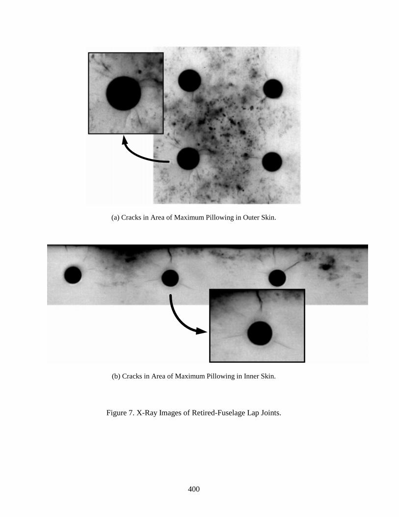
400
(a) Cracks in Area of Maximum Pillowing in Outer Skin.
(b) Cracks in Area of Maximum Pillowing in Inner Skin.
Figure 7. X-Ray Images of Retired-Fuselage Lap Joints.
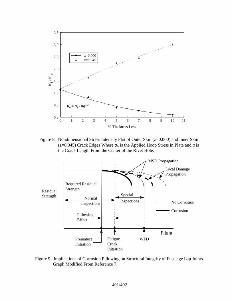
401/402
0 1 2 3 4 5 6 7 8 9 10 11
% Thickness Loss
0.0
0.5
1.0
1.5
2.0
2.5
3.0
3.5
KI /
K o
z=0.000z=0.045
Ko = σh (πa)1/2
Figure 8. Nondimensional Stress Intensity Plot of Outer Skin (z=0.000) and Inner Skin(z=0.045) Crack Edges Where σh is the Applied Hoop Stress in Plate and a isthe Crack Length From the Center of the Rivet Hole.
Flight
ResidualStrength
PillowingEffect
Required ResidualStrength
MSD Propagation
Local DamagePropagation
Special
Inspections
WFDFatigueCrackInitiation
PrematureInitiation
No Corrosion
Corrosion
NormalInspections
Figure 9. Implications of Corrosion Pillowing on Structural Integrity of Fuselage Lap Joints.Graph Modified From Reference 7.
403
IMPROVED NONDESTRUCTIVE INSPECTION TECHNIQUES FORAIRCRAFT INSPECTION
Don Hagemaier and Dwight WilsonMcDonnell Douglas Aerospace
Long Beach, California
ABSTRACT
Through the use of an Integrated Product Team approach and new inspectiontechniques incorporating the latest in imaging capabilities and automation, the costs of somemanpower intensive tasks can now be drastically reduced. Also, through the use of advancededdy current techniques, the detectable size of cracks under flush-head fasteners can bereduced while maintaining a reliable inspection.
Early in this decade, the Federal Aviation Administration (FAA) William J. HughesTechnical Center and the National Aeronautics and Space Administration (NASA) LangleyResearch Center formulated an aging aircraft research plan. The unique aspect about theresearch is that it is driven by the aircraft manufacturers and airlines in order to center only onthose areas in which help is needed and to keep it focused. Once developed, the manufacturerworks with the FAA Aging Aircraft Nondestructive Inspection Validation Center at SandiaNational Laboratories, the airline, and the researcher to transfer technology to the field.
This article first describes the evaluation and results obtained using eddy-currenttechnology to determine the minimum detectable crack size under installed flush-headfasteners. Secondly, it describes the integrated efforts of engineers at McDonnell DouglasAerospace and Northwest Airlines in the successful application of mobile automated scanner(MAUS) eddy-current C-scanning of the DC-10 circumferential and axial crown splices. Theeddy-current C-scanning greatly reduced the man-hour effort required for the existingradiographic inspection. Thirdly, it describes the use of a novel ultrasonic technique coupledto a scanner and graphics for the detection and quantification of corrosion thinning and stresscorrosion cracking of the DC-9 lower wing tee cap. This successful effort resulted from arather large integrated task team. It also results in a vast man-hour savings over the existinginternal visual inspection.
INTRODUCTION
The nondestructive inspection (NDI) portion of the FAA National Aging AircraftResearch Program (NAARP) predicates that improvements must be made to existinginspection techniques and devices so as to provide more reliable detection capabilities. In
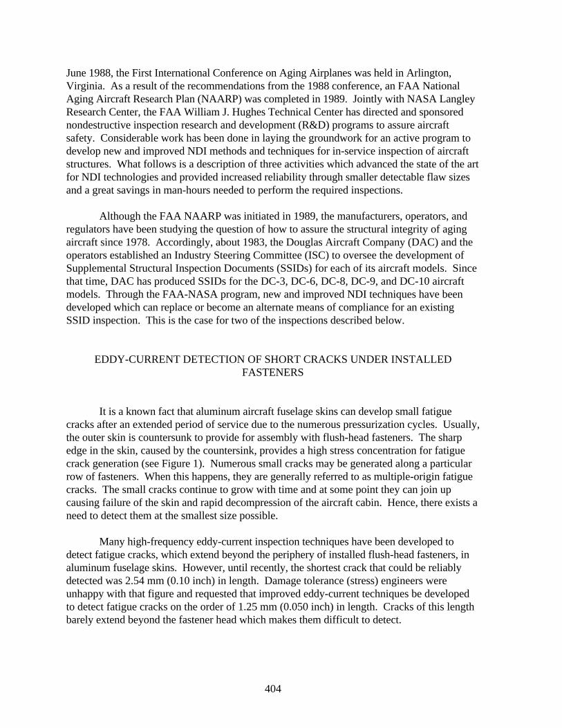
404
June 1988, the First International Conference on Aging Airplanes was held in Arlington,Virginia. As a result of the recommendations from the 1988 conference, an FAA NationalAging Aircraft Research Plan (NAARP) was completed in 1989. Jointly with NASA LangleyResearch Center, the FAA William J. Hughes Technical Center has directed and sponsorednondestructive inspection research and development (R&D) programs to assure aircraftsafety. Considerable work has been done in laying the groundwork for an active program todevelop new and improved NDI methods and techniques for in-service inspection of aircraftstructures. What follows is a description of three activities which advanced the state of the artfor NDI technologies and provided increased reliability through smaller detectable flaw sizesand a great savings in man-hours needed to perform the required inspections.
Although the FAA NAARP was initiated in 1989, the manufacturers, operators, andregulators have been studying the question of how to assure the structural integrity of agingaircraft since 1978. Accordingly, about 1983, the Douglas Aircraft Company (DAC) and theoperators established an Industry Steering Committee (ISC) to oversee the development ofSupplemental Structural Inspection Documents (SSIDs) for each of its aircraft models. Sincethat time, DAC has produced SSIDs for the DC-3, DC-6, DC-8, DC-9, and DC-10 aircraftmodels. Through the FAA-NASA program, new and improved NDI techniques have beendeveloped which can replace or become an alternate means of compliance for an existingSSID inspection. This is the case for two of the inspections described below.
EDDY-CURRENT DETECTION OF SHORT CRACKS UNDER INSTALLEDFASTENERS
It is a known fact that aluminum aircraft fuselage skins can develop small fatiguecracks after an extended period of service due to the numerous pressurization cycles. Usually,the outer skin is countersunk to provide for assembly with flush-head fasteners. The sharpedge in the skin, caused by the countersink, provides a high stress concentration for fatiguecrack generation (see Figure 1). Numerous small cracks may be generated along a particularrow of fasteners. When this happens, they are generally referred to as multiple-origin fatiguecracks. The small cracks continue to grow with time and at some point they can join upcausing failure of the skin and rapid decompression of the aircraft cabin. Hence, there exists aneed to detect them at the smallest size possible.
Many high-frequency eddy-current inspection techniques have been developed todetect fatigue cracks, which extend beyond the periphery of installed flush-head fasteners, inaluminum fuselage skins. However, until recently, the shortest crack that could be reliablydetected was 2.54 mm (0.10 inch) in length. Damage tolerance (stress) engineers wereunhappy with that figure and requested that improved eddy-current techniques be developedto detect fatigue cracks on the order of 1.25 mm (0.050 inch) in length. Cracks of this lengthbarely extend beyond the fastener head which makes them difficult to detect.
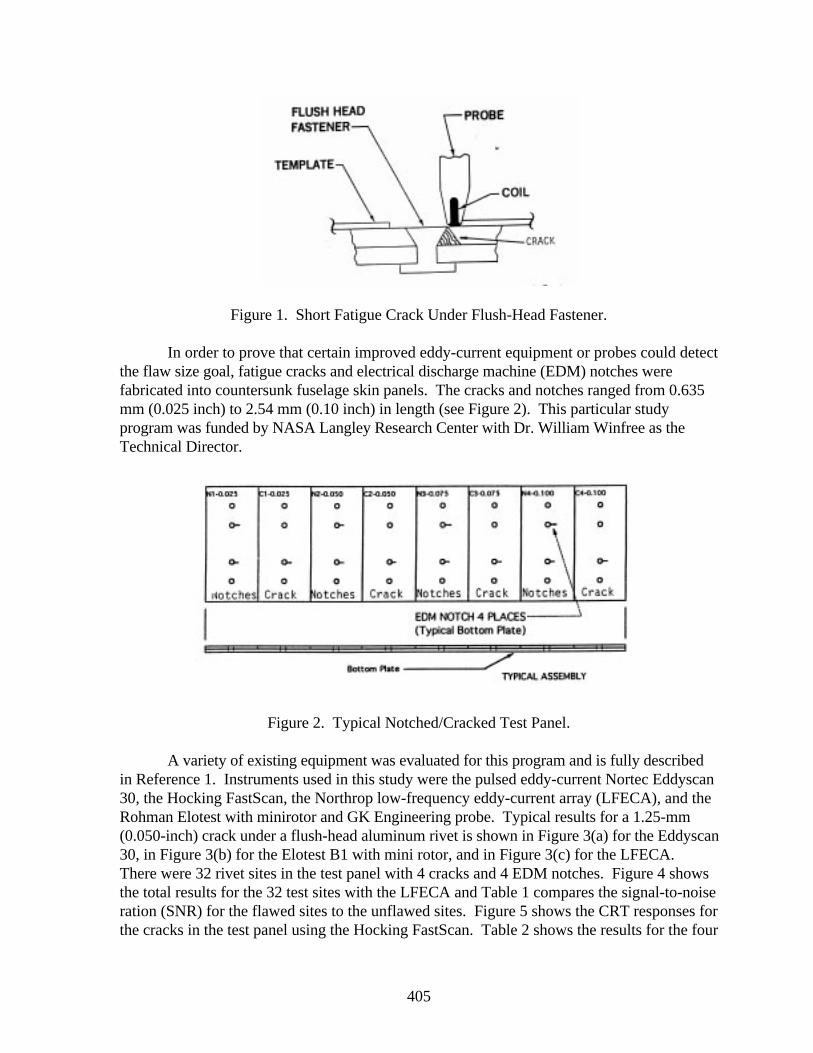
405
Figure 1. Short Fatigue Crack Under Flush-Head Fastener.
In order to prove that certain improved eddy-current equipment or probes could detectthe flaw size goal, fatigue cracks and electrical discharge machine (EDM) notches werefabricated into countersunk fuselage skin panels. The cracks and notches ranged from 0.635mm (0.025 inch) to 2.54 mm (0.10 inch) in length (see Figure 2). This particular studyprogram was funded by NASA Langley Research Center with Dr. William Winfree as theTechnical Director.
Figure 2. Typical Notched/Cracked Test Panel.
A variety of existing equipment was evaluated for this program and is fully describedin Reference 1. Instruments used in this study were the pulsed eddy-current Nortec Eddyscan30, the Hocking FastScan, the Northrop low-frequency eddy-current array (LFECA), and theRohman Elotest with minirotor and GK Engineering probe. Typical results for a 1.25-mm(0.050-inch) crack under a flush-head aluminum rivet is shown in Figure 3(a) for the Eddyscan30, in Figure 3(b) for the Elotest B1 with mini rotor, and in Figure 3(c) for the LFECA.There were 32 rivet sites in the test panel with 4 cracks and 4 EDM notches. Figure 4 showsthe total results for the 32 test sites with the LFECA and Table 1 compares the signal-to-noiseration (SNR) for the flawed sites to the unflawed sites. Figure 5 shows the CRT responses forthe cracks in the test panel using the Hocking FastScan. Table 2 shows the results for the four
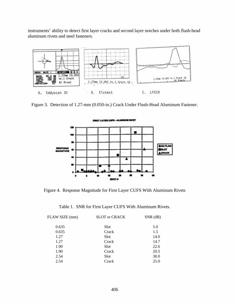
406
instruments’ ability to detect first layer cracks and second layer notches under both flush-headaluminum rivets and steel fasteners.
Figure 3. Detection of 1.27-mm (0.050-in.) Crack Under Flush-Head Aluminum Fastener.
Figure 4. Response Magnitude for First Layer CUFS With Aluminum Rivets
Table 1. SNR for First Layer CUFS With Aluminum Rivets.
FLAW SIZE (mm) SLOT or CRACK SNR (dB)
0.635 Slot 5.00.635 Crack 1.51.27 Slot 14.01.27 Crack 14.71.90 Slot 22.61.90 Crack 20.52.54 Slot 30.02.54 Crack 25.0
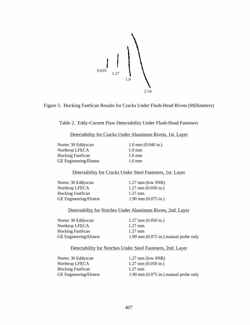
407
Figure 5. Hocking FastScan Results for Cracks Under Flush-Head Rivets (Millimeters)
Table 2. Eddy-Current Flaw Detectability Under Flush-Head Fasteners
Detectability for Cracks Under Aluminum Rivets, 1st. Layer
Nortec 30 Eddyscan 1.0 mm (0.040 in.)Northrop LFECA 1.0 mmHocking FastScan 1.0 mmGE Engineering/Elotest 1.0 mm
Detectability for Cracks Under Steel Fasteners, 1st. Layer
Nortec 30 Eddyscan 1.27 mm (low SNR)Northrop LFECA 1.27 mm (0.050 in.)Hocking FastScan 1.27 mmGE Engineering/Elotest 1.90 mm (0.075 in.)
Detectability for Notches Under Aluminum Rivets, 2nd. Layer
Nortec 30 Eddyscan 1.27 mm (0.050 in.)Northrop LFECA 1.27 mmHocking FastScan 1.27 mmGE Engineering/Elotest 1.90 mm (0.075 in.) manual probe only
Detectability for Notches Under Steel Fasteners, 2nd. Layer
Nortec 30 Eddyscan 1.27 mm (low SNR)Northrop LFECA 1.27 mm (0.050 in.)Hocking FastScan 1.27 mmGE Engineering/Elotest 1.90 mm (0.075 in.) manual probe only
0.6351.27
1.9
2.54
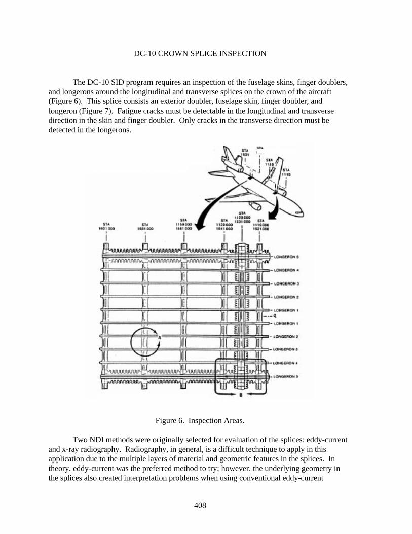
408
DC-10 CROWN SPLICE INSPECTION
The DC-10 SID program requires an inspection of the fuselage skins, finger doublers,and longerons around the longitudinal and transverse splices on the crown of the aircraft(Figure 6). This splice consists an exterior doubler, fuselage skin, finger doubler, andlongeron (Figure 7). Fatigue cracks must be detectable in the longitudinal and transversedirection in the skin and finger doubler. Only cracks in the transverse direction must bedetected in the longerons.
Figure 6. Inspection Areas.
Two NDI methods were originally selected for evaluation of the splices: eddy-currentand x-ray radiography. Radiography, in general, is a difficult technique to apply in thisapplication due to the multiple layers of material and geometric features in the splices. Intheory, eddy-current was the preferred method to try; however, the underlying geometry inthe splices also created interpretation problems when using conventional eddy-current
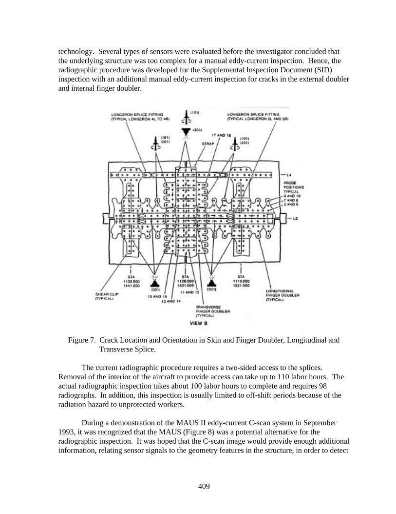
409
technology. Several types of sensors were evaluated before the investigator concluded thatthe underlying structure was too complex for a manual eddy-current inspection. Hence, theradiographic procedure was developed for the Supplemental Inspection Document (SID)inspection with an additional manual eddy-current inspection for cracks in the external doublerand internal finger doubler.
Figure 7. Crack Location and Orientation in Skin and Finger Doubler, Longitudinal andTransverse Splice.
The current radiographic procedure requires a two-sided access to the splices.Removal of the interior of the aircraft to provide access can take up to 110 labor hours. Theactual radiographic inspection takes about 100 labor hours to complete and requires 98radiographs. In addition, this inspection is usually limited to off-shift periods because of theradiation hazard to unprotected workers.
During a demonstration of the MAUS II eddy-current C-scan system in September1993, it was recognized that the MAUS (Figure 8) was a potential alternative for theradiographic inspection. It was hoped that the C-scan image would provide enough additionalinformation, relating sensor signals to the geometry features in the structure, in order to detect
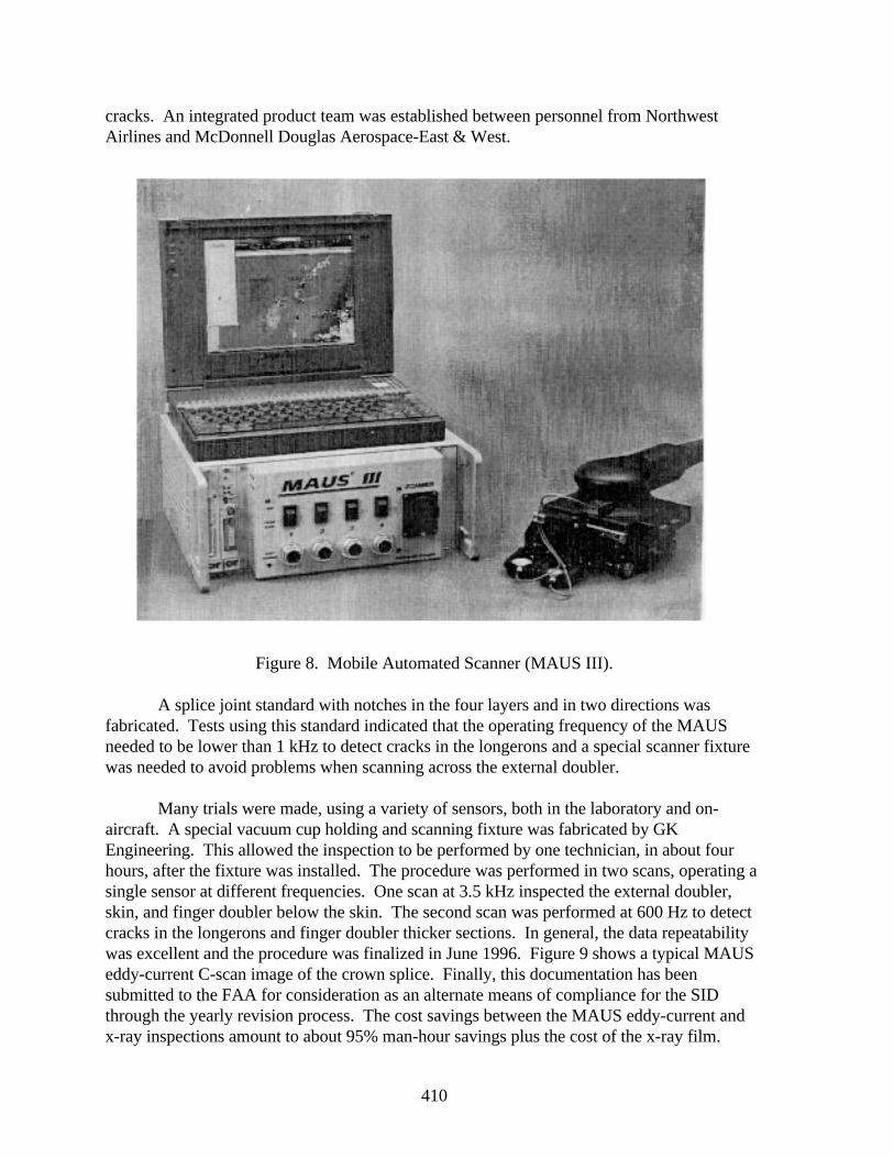
410
cracks. An integrated product team was established between personnel from NorthwestAirlines and McDonnell Douglas Aerospace-East & West.
Figure 8. Mobile Automated Scanner (MAUS III).
A splice joint standard with notches in the four layers and in two directions wasfabricated. Tests using this standard indicated that the operating frequency of the MAUSneeded to be lower than 1 kHz to detect cracks in the longerons and a special scanner fixturewas needed to avoid problems when scanning across the external doubler.
Many trials were made, using a variety of sensors, both in the laboratory and on-aircraft. A special vacuum cup holding and scanning fixture was fabricated by GKEngineering. This allowed the inspection to be performed by one technician, in about fourhours, after the fixture was installed. The procedure was performed in two scans, operating asingle sensor at different frequencies. One scan at 3.5 kHz inspected the external doubler,skin, and finger doubler below the skin. The second scan was performed at 600 Hz to detectcracks in the longerons and finger doubler thicker sections. In general, the data repeatabilitywas excellent and the procedure was finalized in June 1996. Figure 9 shows a typical MAUSeddy-current C-scan image of the crown splice. Finally, this documentation has beensubmitted to the FAA for consideration as an alternate means of compliance for the SIDthrough the yearly revision process. The cost savings between the MAUS eddy-current andx-ray inspections amount to about 95% man-hour savings plus the cost of the x-ray film.
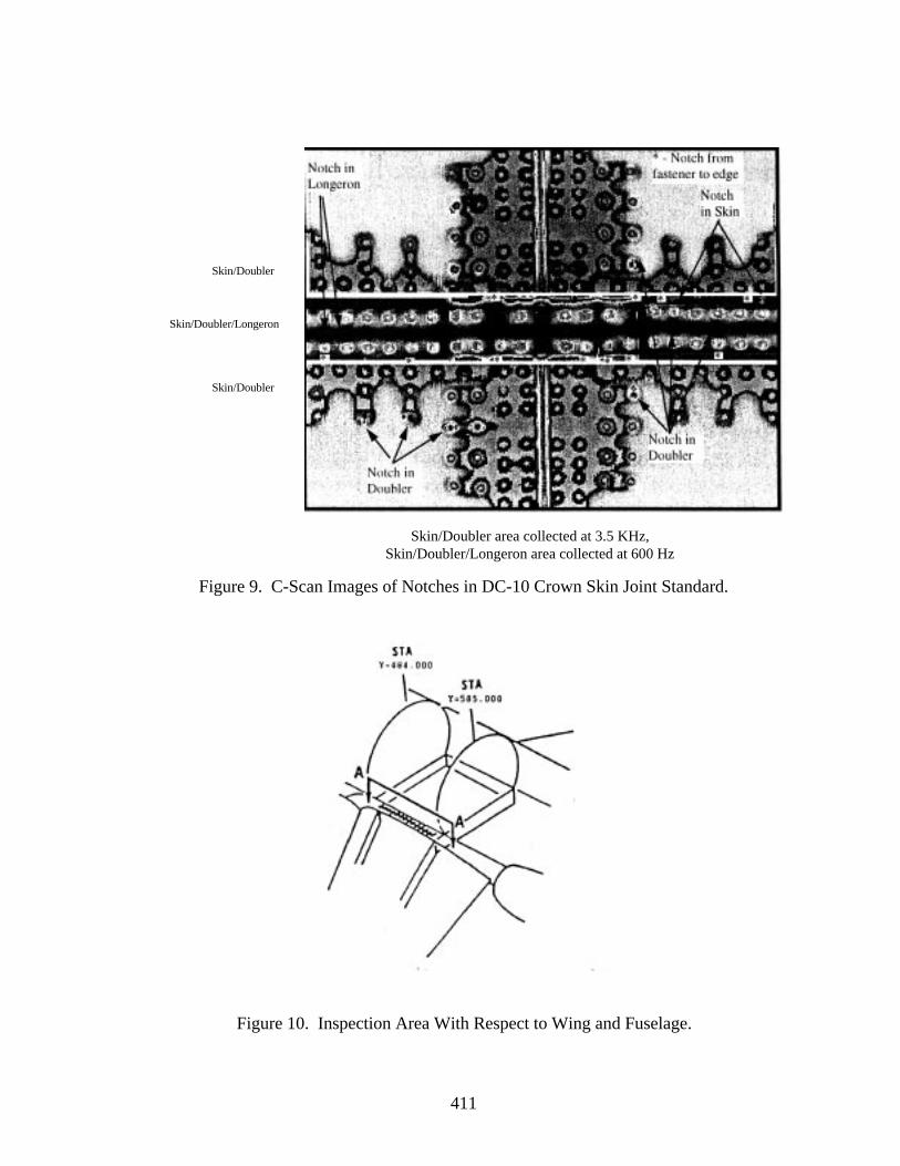
411
Skin/Doubler area collected at 3.5 KHz,Skin/Doubler/Longeron area collected at 600 Hz
Figure 9. C-Scan Images of Notches in DC-10 Crown Skin Joint Standard.
Figure 10. Inspection Area With Respect to Wing and Fuselage.
Skin/Doubler
Skin/Doubler/Longeron
Skin/Doubler
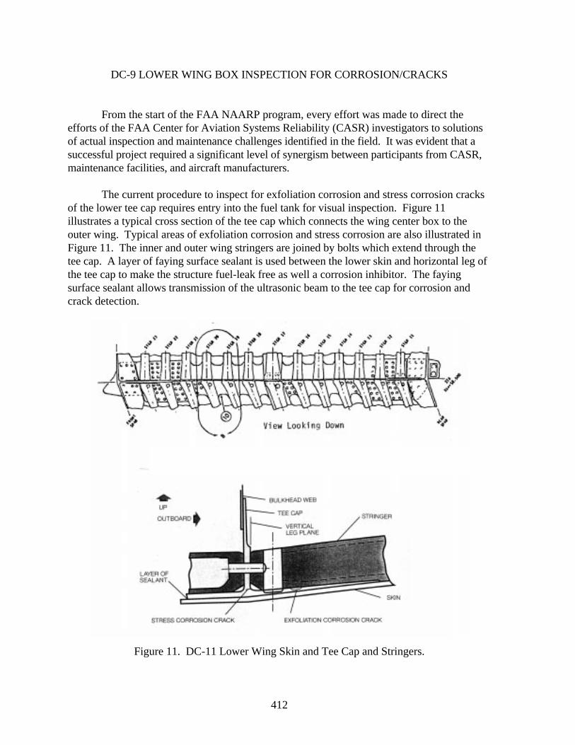
412
DC-9 LOWER WING BOX INSPECTION FOR CORROSION/CRACKS
From the start of the FAA NAARP program, every effort was made to direct theefforts of the FAA Center for Aviation Systems Reliability (CASR) investigators to solutionsof actual inspection and maintenance challenges identified in the field. It was evident that asuccessful project required a significant level of synergism between participants from CASR,maintenance facilities, and aircraft manufacturers.
The current procedure to inspect for exfoliation corrosion and stress corrosion cracksof the lower tee cap requires entry into the fuel tank for visual inspection. Figure 11illustrates a typical cross section of the tee cap which connects the wing center box to theouter wing. Typical areas of exfoliation corrosion and stress corrosion are also illustrated inFigure 11. The inner and outer wing stringers are joined by bolts which extend through thetee cap. A layer of faying surface sealant is used between the lower skin and horizontal leg ofthe tee cap to make the structure fuel-leak free as well a corrosion inhibitor. The fayingsurface sealant allows transmission of the ultrasonic beam to the tee cap for corrosion andcrack detection.
Figure 11. DC-11 Lower Wing Skin and Tee Cap and Stringers.
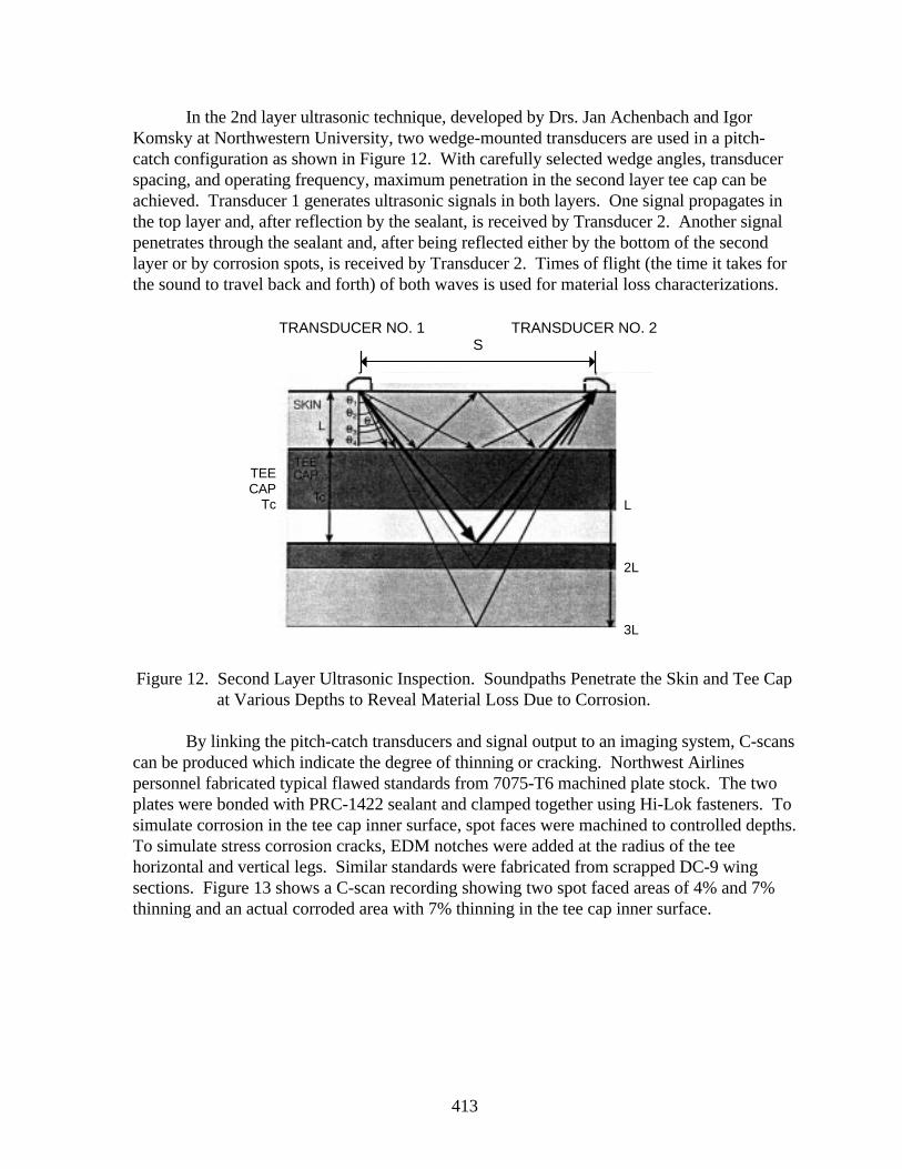
413
In the 2nd layer ultrasonic technique, developed by Drs. Jan Achenbach and IgorKomsky at Northwestern University, two wedge-mounted transducers are used in a pitch-catch configuration as shown in Figure 12. With carefully selected wedge angles, transducerspacing, and operating frequency, maximum penetration in the second layer tee cap can beachieved. Transducer 1 generates ultrasonic signals in both layers. One signal propagates inthe top layer and, after reflection by the sealant, is received by Transducer 2. Another signalpenetrates through the sealant and, after being reflected either by the bottom of the secondlayer or by corrosion spots, is received by Transducer 2. Times of flight (the time it takes forthe sound to travel back and forth) of both waves is used for material loss characterizations.
Figure 12. Second Layer Ultrasonic Inspection. Soundpaths Penetrate the Skin and Tee Cap at Various Depths to Reveal Material Loss Due to Corrosion.
By linking the pitch-catch transducers and signal output to an imaging system, C-scanscan be produced which indicate the degree of thinning or cracking. Northwest Airlinespersonnel fabricated typical flawed standards from 7075-T6 machined plate stock. The twoplates were bonded with PRC-1422 sealant and clamped together using Hi-Lok fasteners. Tosimulate corrosion in the tee cap inner surface, spot faces were machined to controlled depths.To simulate stress corrosion cracks, EDM notches were added at the radius of the teehorizontal and vertical legs. Similar standards were fabricated from scrapped DC-9 wingsections. Figure 13 shows a C-scan recording showing two spot faced areas of 4% and 7%thinning and an actual corroded area with 7% thinning in the tee cap inner surface.
TEECAP
Tc
TRANSDUCER NO. 1 TRANSDUCER NO. 2S
L
2L
3L
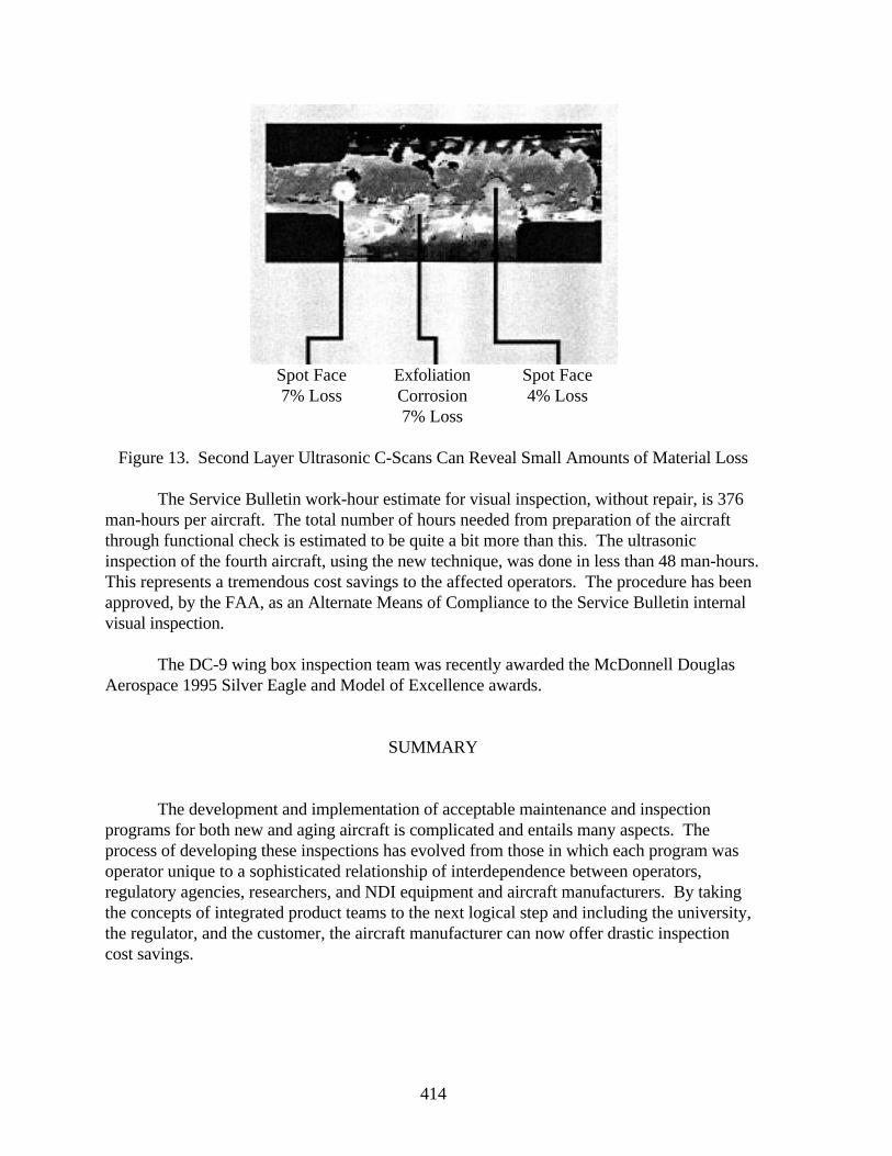
414
Spot Face7% Loss
ExfoliationCorrosion7% Loss
Spot Face4% Loss
Figure 13. Second Layer Ultrasonic C-Scans Can Reveal Small Amounts of Material Loss
The Service Bulletin work-hour estimate for visual inspection, without repair, is 376man-hours per aircraft. The total number of hours needed from preparation of the aircraftthrough functional check is estimated to be quite a bit more than this. The ultrasonicinspection of the fourth aircraft, using the new technique, was done in less than 48 man-hours.This represents a tremendous cost savings to the affected operators. The procedure has beenapproved, by the FAA, as an Alternate Means of Compliance to the Service Bulletin internalvisual inspection.
The DC-9 wing box inspection team was recently awarded the McDonnell DouglasAerospace 1995 Silver Eagle and Model of Excellence awards.
SUMMARY
The development and implementation of acceptable maintenance and inspectionprograms for both new and aging aircraft is complicated and entails many aspects. Theprocess of developing these inspections has evolved from those in which each program wasoperator unique to a sophisticated relationship of interdependence between operators,regulatory agencies, researchers, and NDI equipment and aircraft manufacturers. By takingthe concepts of integrated product teams to the next logical step and including the university,the regulator, and the customer, the aircraft manufacturer can now offer drastic inspectioncost savings.
415/416
ACKNOWLEDGMENT
The authors would like to express their thanks to the teams who accomplished thesetechnology advances:
Special thanks to Dr. Ed Generazio and Dr. William Winfree, of NASALangley Research Center (LaRC) for providing funding for the cracks underfastener study.
Special thanks to Nancy Wood of MDA East, Bill Jappe of MDA West,and Maurice Johnson of Northwest Airlines for completing the MAUS eddy-current C-scan inspection for the DC-10 crown splices.
Special thanks to the DC-9 Wing Box Team consisting of Igor Komskyand Jan Achenbach of Northwestern University; Jeff Register and Greg Kinkertof Northwest Airlines; Al Steinberg and Gerardo Hueto of McDonnell Douglas;Glen Andrew, Bob Grills, and Mike Ashbaugh of SAIC; David Moore of theFAA Aging Aircraft Nondestructive Inspection Validation Center at SandiaNational Laboratories; and Hans Weber of Weber Technology Applications.
REFERENCES
1. Hagemaier, D.: “Eddy Current Detection of Short Cracks Under Installed Fasteners,”1995 ATA NDT Forum, Hartford, Connecticut.
2. Jappe, W., Johnson, M., and Wood, N.: “The Transition Process from Emerging
NDT Technology to Production Inspection Application.” 1995 ATA NDT Forum,Hartford, Connecticut.
3. Komsky, I. N., Achenbach, J. D., Andrew, G., Grills, R., Register, J., Linkert, G.,
Hueto, G. M., Steinberg, A., Ashbaugh, M., Moore, D. G., and Weber, H.: “AnUltrasonic Technique to Detect Corrosion in DC-9 Wing Box From Concept to FieldApplication,” Materials Evaluation, July 1995, pp. 848-852.
417
IM PROVING THE DAMAGE TOLERANCE O F BONDEDSTRUCTURES VIA ADHESIVE LAYER BARRIERS
Dr. John C. BrewerVolpe National Transportation Systems Center
Cambridge, MA 02142-1093
ABSTRACT
Modern aircraft possess numerous applications for structural adhesive bonding.Continued airworthiness of these applications requires tolerance of undetected damage suchas debonding. A serious concern is that a partial debond could grow unstably across theentire bond. For example, composite patch repairs of structural cracks can be extremelyeffective at retarding crack growth, yet they need a damage tolerant bonding mechanism thatmaintains the patch’s utility even after partial bond failure. Analysis is presented that showsthat a composite patch on a cracked aluminum sheet will still be effective even if a largeportion of the bonded area has debonded, as long as the remaining bonded region is stableand the patch still provides a viable load path around the crack. A method is proposed whichenhances the damage tolerance of a bond with barriers that divide the adhesive layer intodiscrete regions. The barriers are inserted into the adhesive bond layer before curing andmake uninterrupted contact with both adherends, thereby forming separate zones of adhesive.The barriers may be constructed of a nonstick material and may be slightly thicker than thenominal adhesive layer. If a local debond were to grow to a barrier, the debond front shouldpreferentially travel along the lower energy bond between the adhesive and the barrier ratherthan through the adhesive or along an adhesive/adherend interface. The barriers shouldprevent the extension of the debond from one region to the next. Since most load istransferred in a boundary region near the edge of a bond, dividing the bond into severalregions should make it sufficiently redundant to withstand locally unstable debond growth.
INTRODUCTION
Any evaluation of aircraft structural integrity must consider the long-term ability towithstand reasonably expected loads after damage has occurred. Prudent engineeringprinciples suggest the use of redundant structures and redundant joining methods. TheFederal Aviation Administration requires that transport category aircraft be “damagetolerant.” That is, they must be
“evaluated to ensure that should serious fatigue, corrosion, or accidentaldamage occur within the operational life of the airplane, the remainingstructure can withstand reasonable loads without failure or excessivestructural deformation until the damage is detected. ” [1]
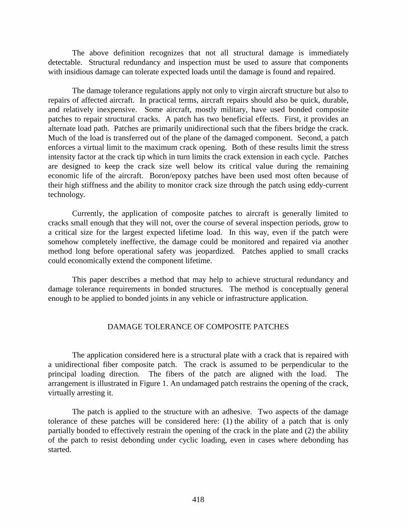
418
The above definition recognizes that not all structural damage is immediatelydetectable. Structural redundancy and inspection must be used to assure that componentswith insidious damage can tolerate expected loads until the damage is found and repaired.
The damage tolerance regulations apply not only to virgin aircraft structure but also torepairs of affected aircraft. In practical terms, aircraft repairs should also be quick, durable,and relatively inexpensive. Some aircraft, mostly military, have used bonded compositepatches to repair structural cracks. A patch has two beneficial effects. First, it provides analternate load path. Patches are primarily unidirectional such that the fibers bridge the crack.Much of the load is transferred out of the plane of the damaged component. Second, a patchenforces a virtual limit to the maximum crack opening. Both of these results limit the stressintensity factor at the crack tip which in turn limits the crack extension in each cycle. Patchesare designed to keep the crack size well below its critical value during the remainingeconomic life of the aircraft. Boron/epoxy patches have been used most often because oftheir high stiffness and the ability to monitor crack size through the patch using eddy-currenttechnology.
Currently, the application of composite patches to aircraft is generally limited tocracks small enough that they will not, over the course of several inspection periods, grow toa critical size for the largest expected lifetime load. In this way, even if the patch weresomehow completely ineffective, the damage could be monitored and repaired via anothermethod long before operational safety was jeopardized. Patches applied to small crackscould economically extend the component lifetime.
This paper describes a method that may help to achieve structural redundancy anddamage tolerance requirements in bonded structures. The method is conceptually generalenough to be applied to bonded joints in any vehicle or infrastructure application.
DAMAGE TOLERANCE OF COMPOSITE PATCHES
The application considered here is a structural plate with a crack that is repaired witha unidirectional fiber composite patch. The crack is assumed to be perpendicular to theprincipal loading direction. The fibers of the patch are aligned with the load. Thearrangement is illustrated in Figure 1. An undamaged patch restrains the opening of the crack,virtually arresting it.
The patch is applied to the structure with an adhesive. Two aspects of the damagetolerance of these patches will be considered here: (1) the ability of a patch that is onlypartially bonded to effectively restrain the opening of the crack in the plate and (2) the abilityof the patch to resist debonding under cyclic loading, even in cases where debonding hasstarted.
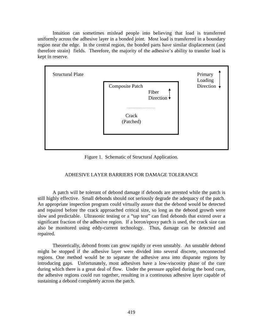
419
Intuition can sometimes mislead people into believing that load is transferreduniformly across the adhesive layer in a bonded joint. Most load is transferred in a boundaryregion near the edge. In the central region, the bonded parts have similar displacement (andtherefore strain) fields. Therefore, the majority of the adhesive’s ability to transfer load iskept in reserve.
Structural Plate PrimaryLoading
Composite Patch DirectionFiberDirection
Crack(Patched)
Figure 1. Schematic of Structural Application.
ADHESIVE LAYER BARRIERS FOR DAMAGE TOLERANCE
A patch will be tolerant of debond damage if debonds are arrested while the patch isstill highly effective. Small debonds should not seriously degrade the adequacy of the patch.An appropriate inspection program could virtually assure that the debond would be detectedand repaired before the crack approached critical size, so long as the debond growth wereslow and predictable. Ultrasonic testing or a “tap test” can find debonds that extend over asignificant fraction of the adhesive region. If a boron/epoxy patch is used, the crack size canalso be monitored using eddy-current technology. Thus, damage can be detected andrepaired.
Theoretically, debond fronts can grow rapidly or even unstably. An unstable debondmight be stopped if the adhesive layer were divided into several discrete, unconnectedregions. One method would be to separate the adhesive area into disparate regions byintroducing gaps. Unfortunately, most adhesives have a low-viscosity phase of the cureduring which there is a great deal of flow. Under the pressure applied during the bond cure,the adhesive regions could run together, resulting in a continuous adhesive layer capable ofsustaining a debond completely across the patch.
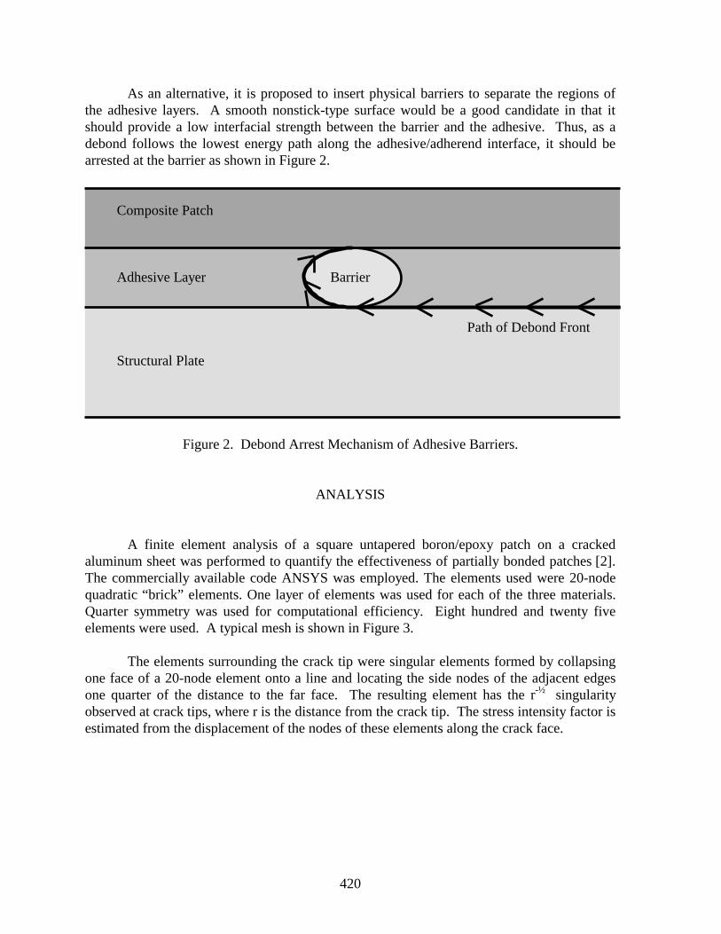
420
As an alternative, it is proposed to insert physical barriers to separate the regions ofthe adhesive layers. A smooth nonstick-type surface would be a good candidate in that itshould provide a low interfacial strength between the barrier and the adhesive. Thus, as adebond follows the lowest energy path along the adhesive/adherend interface, it should bearrested at the barrier as shown in Figure 2.
Composite Patch
Adhesive Layer Barrier
Path of Debond Front
Structural Plate
Figure 2. Debond Arrest Mechanism of Adhesive Barriers.
ANALYSIS
A finite element analysis of a square untapered boron/epoxy patch on a crackedaluminum sheet was performed to quantify the effectiveness of partially bonded patches [2].The commercially available code ANSYS was employed. The elements used were 20-nodequadratic “brick” elements. One layer of elements was used for each of the three materials.Quarter symmetry was used for computational efficiency. Eight hundred and twenty fiveelements were used. A typical mesh is shown in Figure 3.
The elements surrounding the crack tip were singular elements formed by collapsingone face of a 20-node element onto a line and locating the side nodes of the adjacent edgesone quarter of the distance to the far face. The resulting element has the r-½ singularityobserved at crack tips, where r is the distance from the crack tip. The stress intensity factor isestimated from the displacement of the nodes of these elements along the crack face.
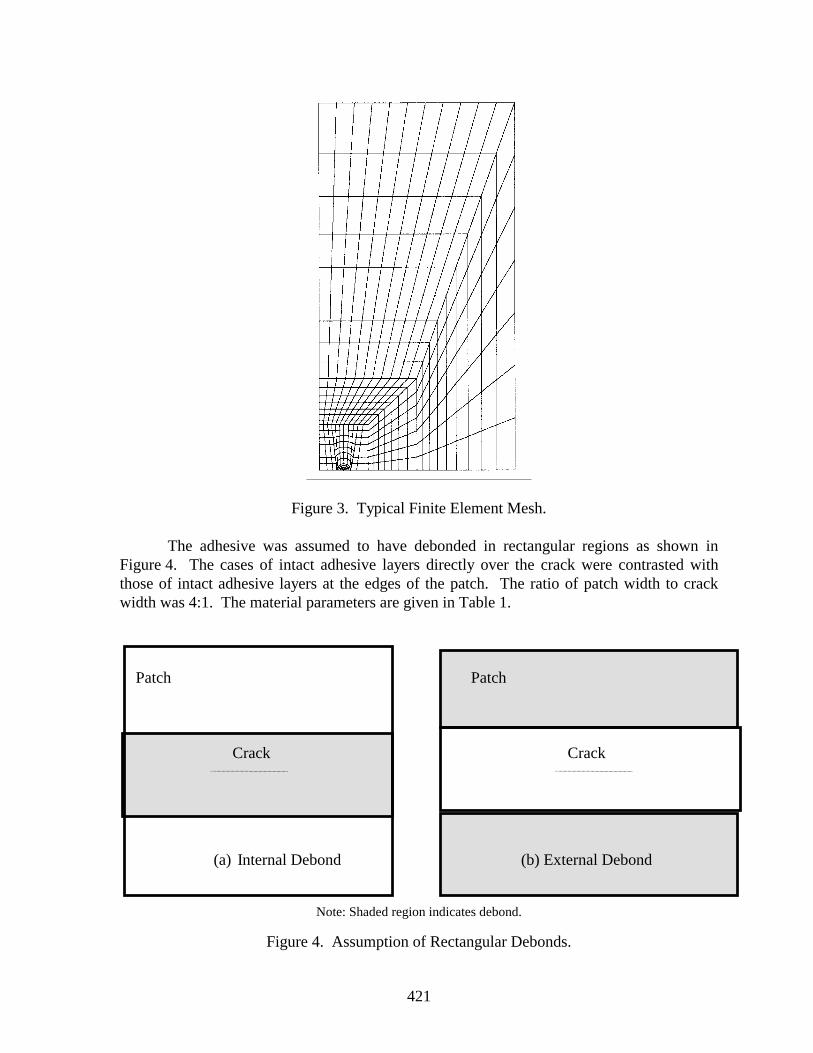
421
Figure 3. Typical Finite Element Mesh.
The adhesive was assumed to have debonded in rectangular regions as shown inFigure 4. The cases of intact adhesive layers directly over the crack were contrasted withthose of intact adhesive layers at the edges of the patch. The ratio of patch width to crackwidth was 4:1. The material parameters are given in Table 1.
Patch Patch
Crack Crack
(a) Internal Debond (b) External Debond
Note: Shaded region indicates debond.
Figure 4. Assumption of Rectangular Debonds.
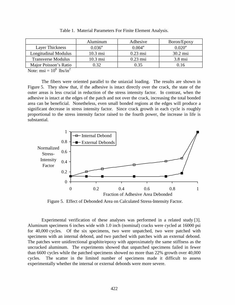
422
Table 1. Material Parameters For Finite Element Analysis.
Aluminum Adhesive Boron/EpoxyLayer Thickness 0.036″ 0.004″ 0.020″
Longitudinal Modulus 10.3 msi 0.23 msi 30.2 msiTransverse Modulus 10.3 msi 0.23 msi 3.8 msi
Major Poisson’s Ratio 0.32 0.35 0.16Note: msi = 106 lbs/in2
The fibers were oriented parallel to the uniaxial loading. The results are shown inFigure 5. They show that, if the adhesive is intact directly over the crack, the state of theouter areas is less crucial in reduction of the stress intensity factor. In contrast, when theadhesive is intact at the edges of the patch and not over the crack, increasing the total bondedarea can be beneficial. Nonetheless, even small bonded regions at the edges will produce asignificant decrease in stress intensity factor. Since crack growth in each cycle is roughlyproportional to the stress intensity factor raised to the fourth power, the increase in life issubstantial.
Figure 5. Effect of Debonded Area on Calculated Stress-Intensity Factor.
0
0.2
0.4
0.6
0.8
1
0 0.2 0.4 0.6 0.8 1Fraction of Adhesive Area Debonded
NormalizedStress-
IntensityFactor
Internal Debond
External Debonds
Experimental verification of these analyses was performed in a related study [3].Aluminum specimens 6 inches wide with 1.0 inch (nominal) cracks were cycled at 16000 psifor 40,000 cycles. Of the six specimens, two were unpatched, two were patched withspecimens with an internal debond, and two patched with patches with an external debond.The patches were unidirectional graphite/epoxy with approximately the same stiffness as theuncracked aluminum. The experiments showed that unpatched specimens failed in fewerthan 6600 cycles while the patched specimens showed no more than 22% growth over 40,000cycles. The scatter in the limited number of specimens made it difficult to assessexperimentally whether the internal or external debonds were more severe.
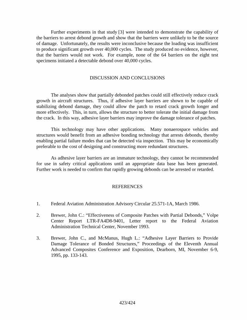
423/424
Further experiments in that study [3] were intended to demonstrate the capability ofthe barriers to arrest debond growth and show that the barriers were unlikely to be the sourceof damage. Unfortunately, the results were inconclusive because the loading was insufficientto produce significant growth over 40,000 cycles. The study produced no evidence, however,that the barriers would not work. For example, none of the 64 barriers on the eight testspecimens initiated a detectable debond over 40,000 cycles.
DISCUSSION AND CONCLUSIONS
The analyses show that partially debonded patches could still effectively reduce crackgrowth in aircraft structures. Thus, if adhesive layer barriers are shown to be capable ofstabilizing debond damage, they could allow the patch to retard crack growth longer andmore effectively. This, in turn, allows the structure to better tolerate the initial damage fromthe crack. In this way, adhesive layer barriers may improve the damage tolerance of patches.
This technology may have other applications. Many nonaerospace vehicles andstructures would benefit from an adhesive bonding technology that arrests debonds, therebyenabling partial failure modes that can be detected via inspection. This may be economicallypreferable to the cost of designing and constructing more redundant structures.
As adhesive layer barriers are an immature technology, they cannot be recommendedfor use in safety critical applications until an appropriate data base has been generated.Further work is needed to confirm that rapidly growing debonds can be arrested or retarded.
REFERENCES
1. Federal Aviation Administration Advisory Circular 25.571-1A, March 1986. 2. Brewer, John C.: “Effectiveness of Composite Patches with Partial Debonds,” Volpe
Center Report LTR-FA4D8-9401, Letter report to the Federal AviationAdministration Technical Center, November 1993.
3. Brewer, John C., and McManus, Hugh L.: “Adhesive Layer Barriers to Provide
Damage Tolerance of Bonded Structures,” Proceedings of the Eleventh AnnualAdvanced Composites Conference and Exposition, Dearborn, MI, November 6-9,1995, pp. 133-143.
425
IN SEARCH OF THE HOLY GRAILTHE DETERMINISTIC PREDICTION OF DAMAGE
Digby D. Macdonald and Jose MagalhaesThe Pennsylvania State University
Center for Advanced Materials517 Deike Building
University Park, PA 16802USA
ABSTRACT
The development of fatigue and corrosion fatigue damage, and of other forms oflocalized corrosion damage, in aircraft structures is generally described in terms of damagetolerance methods in which the fatigue data are incorporated as empirical crack growthrate/stress intensity (range) correlations, and the corrosion information is either ignored or isincluded on an ad hoc basis. However, the prediction of corrosion damage in other industries(e.g., the electric power industry) is gradually yielding to determinism, which allows muchmore robust predictions of failure times to be made. In this paper, we review thedeterministic methods and explore the prospects for developing similar techniques forpredicting failures in aircraft structures.
INTRODUCTION
The prediction of service-induced damage (pitting, fatigue, corrosion fatigue, andgeneral corrosion) in aircraft structures is currently made on the basis of empirical and semi-empirical methods in which laboratory data (e.g., da/dN vs. ∆K for cyclic crack growth) areused to estimate metal loss and crack extension rates under preselected conditions. Thesepredictions are then combined with periodic in-service inspections, within the framework ofthe damage tolerance philosophy, to assess and track the progression of damage. While thefracture mechanics basis for this procedure is well-developed, the corrosion aspects areincorporated on an ad hoc basis, with the result that our ability to predict the evolution ofdamage as a function of operating conditions is poor.
In this paper, a detailed analysis is presented of methods that have been developed inother areas of science and engineering (e.g., in the nuclear power industry) fordeterministically predicting corrosion damage, with particular emphasis on the prospects ofapplying these techniques to aircraft. These methods appeal to the natural laws (conservationof charge, Faraday’s law, etc.) for their predictive rigor and provide an opportunity foraccurate damage prediction, provided that future operating conditions can be envisioned andspecified. In the general case, which will be emphasized, the progression of damage is
426
described as arising from a progressive nucleation/growth/death process. Thus, for a singleevent (e.g., a pit or crack), these three phases occur sequentially, each of which is amenableto deterministic modeling, but for an ensemble of events, the extent of damage developscollectively in a parallel manner. This scenario is most effectively described in terms of adamage function, which is the distribution in the damaging parameter (e.g., pit or cracklength) as a function of exposure conditions and observation time. The damage functionprovides a convenient mathematical basis for defining “failure time,” “service life,”“corrosion allowance,” “probability of failure,” and many other such terms and concepts thatenter into life prediction for complex engineering structures.
THE TEMPORAL DEVELOPMENT OF DAMAGE
The development of damage, regardless of the details of the processes involved, isbest described as a progressive nucleation/growth/death process. Such processes arecharacterized by the nucleation of new damage as existing damage grows and dies, with theresult that the damage is distributed. The most convenient way of expressing damage is inthe form of a damage function,1 which is a histogram of frequency versus depth for a givenobservation time (t1, t2, or t3), as shown in Figure 1. These functions display the generaltrends that are seen in experimental damage functions as well as those that are predictedtheoretically, including:
1. The total damage, as represented by the area, increases with increasing observation time. 2. The upper extreme of the damage function extends to greater depths with increasing
observation time. 3. The distribution may be multimodal only if more than one nucleation phenomenon is
present and only then if the kinetics of nucleation are temporally separated.
For most purposes, we are interested in estimating failure times, and DFA (Damage FunctionAnalysis) allows us to do that by specifying a failure criterion. In many cases, this criterionwill be a critical dimension (Lcrit, Figure 1), corresponding perhaps to the thickness of a pipewall or to an acceptable “corrosion allowance”. However, the criterion may be less(physically) direct. For example, in specifying failure for systems that exhibit stresscorrosion cracking or corrosion fatigue, it is necessary to specify a critical stress intensityfactor, KI, such that KI > KIC, where KIC is the fracture toughness, corresponding to conditionsfor unstable (fast) fracture. In this case, the failure criterion is a function of other systemparameters, including stress and geometry. Thus, with reference to Figure 1, Lcrit willdecrease as the stress is made larger, so that damage that was subcritical at one stress levelmay become supercritical at another. This is clearly an important issue for aircraft, wherewide ranges of stress are experienced during operation.
Returning again to Figure 1, it is important to note that the most damaging events(defined here as being the deepest) are generally the first to nucleate and/or the last to die,

427
and the least damaging events are those that are last to nucleate and/or the first to die. In anyevent, a deterministic prediction of the evolution of damage, and hence estimation of thefailure time, must address all three constitutive phenomena; nucleation, growth, and death.These phenomena must be described in a manner that recognizes their serial relationships fora single event (birth → growth → death) but that they occur in parallel for an ensemble ofevents.
The Nucleation of Damage
The initial fundamental event in the nucleation of localized corrosion damage (e.g.,that due to pitting, stress corrosion cracking, and corrosion fatigue) is passivity breakdownand the eventual establishment of a highly nonuniform current distribution withinmicroscopic dimensions of the nucleation point. As a result of an intensive effort over thepast decade to develop an understanding of the breakdown of passive films, we have derivedtheoretical distribution functions for passivity breakdown that are in good agreement withexperiment2-6. We derived these distribution functions from our point defect model (PDM)for the growth and breakdown of passive films by assuming that breakdown occurs when acritical concentration of cation vacancies accumulates locally at the metal/passive-filminterface such that decohesion occurs between the barrier layer and the metal substrate.Subsequently, localized dissolution and/or mechanical instability leads to rupture of the film.2
We further assumed that the breakdown sites are normally distributed with respect to thediffusivity of cation vacancies within the film.3-5 The full derivation of these distributionfunctions can be found in the literature.2-6
From the PDM,2 the breakdown voltage and the induction time for a single pitnucleation site on the surface are given by
Vc = 4.606RTχαF
logJm
Jo ˆ u − χ / 2
− 2.303RTαF
log ax( ) (1)
and
tind = ′ ξ expχαF∆V
2RT
−1
−1
+τ (2)
respectively, where χ is the film stoichiometry MOχ / 2( ), α is the dependence of the
potential drop across the film/solution interface on applied voltage, ax is the activity ofhalide ion in the solution, τ is a relaxation time (τ ~ 0), ∆V = V − Vc , V is the applied
voltage (or the corrosion potential under open circuit conditions), Jo = ˆ a D, and theparameters a ,u , and Jm are defined in the original derivation2.
Assuming that the breakdown sites are normally distributed in terms of the cationvacancy diffusivity,
428
dN
dD=
1
2πσ D
exp − D − D ( )2
/ 2σ D2[ ] (3)
where D is the mean diffusivity and σD is the standard deviation, the PDM yields thedistributions in the breakdown voltage and induction time:3-6
dN
dVc
= −ˆ γ D
2πσ D
⋅ e− D − D ( )2 / 2σ D2
(4)
anddN
dtind
=ξuχ / 2
2πσ Dˆ a
e− D − D ( )2 / 2σ D
2
⋅e− ˆ γ V
axχ / 2 tind −τ( )2 (5)
where γ = χFα / 2RT. Equations 4 and 5 contain four important system parameters; D andσD , which describe the transport properties of cation vacancies in the passive film, and αand β , which appear in the expression for the dependence of the potential drop across thefilm/solution interface on applied voltage and pH, i.e., φ f / s = αV + βpH + φ f / s
o , where φ f / so is
a constant. All four parameters can be determined by independent experiment: D fromelectrochemical impedance spectroscopy, σD from passivity breakdown induction timemeasurements,2 and α and β from film growth data, some of which exists in the literature.
The Growth of Damage
The growth of damage due to localized corrosion is an electrochemical phenomenon,and any model that purports to be deterministic must conserve charge and obey Faraday’slaw, which are the two governing natural laws.7-13 Accordingly, with reference to Figure 2,
the conservation of charge requires that i dSS∫ = 0, where i is the current density on surface
element dS, with the integral being evaluated over the entire surface, including the creviceinternal and external surfaces, where anodic (metal oxidation) and cathodic (e.g., oxygenreduction) reactions predominate, respectively. Thus, solution of Laplace’s (or more strictly,Poisson’s) equation for the appropriate boundary conditions, subject to the constraint
imposed by i dSS∫ = 0, yields the potential and current distributions within the system.
Knowledge of the current density (it ) at the crevice base (pit or crack) therefore yields theextension rate according to Faraday’s law as dL dt= M it 2ρm z F, where M and z are thecomposition-averaged (for alloys) atomic weight and oxidation number, respectively, ρm isthe density of the alloy, and F is Faraday’s constant. Differentiation between pit growth andcrack growth is accomplished by noting that, in the latter, the oxidation current density isstrain-rate dependent. It is important to note that even though all of the mechanistic details inthese “coupled environment” models may not be correct, they are deterministic in the globalsense and hence, in principle, are capable of providing for robust prediction.
429
Death
Perhaps the most difficult phenomenon to deal with in localized corrosion is the deathof an individual event (pit or crack), principally because most attention has been focused onnucleation rather than on describing the ultimate fate of a crevice. However, it is now knownthat two quite distinct “death” phenomena need to be defined: (i) prompt repassivation, and(ii) delayed repassivation. Prompt repassivation occurs when the crevice nucleus that isproduced by passivity breakdown fails to attain conditions that permit sustained growth. Thenecessary conditions for transition from metastable to stable pitting for stainless steels havebeen expressed in terms of a pit stability product (PSP)14-17 as14 0.6mA/ cm> i a > 0.3mA/ cm,where i is the current density at the pit nucleus surface of radius a (hemisphericalgeometry). The lower limit is imposed by the need to establish sufficiently aggressiveconditions that pit growth is sustained, whereas the upper limit is defined by the solubility ofthe salt. Average lifetimes for metastable pits depend on the properties of the substrate andthe environment but are typically less than one second.
The second death phenomenon, “delayed repassivation,” is responsible for the deathof stable pits, i.e., the repassivation of those pits that satisfy Equation 12, over much longertimes. The kinetics and mechanisms of this process are poorly defined or understood, butnumerous causes might be postulated, including changes in the properties of the environment(pH, corrosion potential, flow velocity, etc.). At the present time, delayed repassivationappears to be best described as a first order decay process, − dN dt = kr N , where N is thenumber of active (surviving) pits, and kr is the rate constant. No theory currently exists thatallows one to calculate kr from first principles; instead, the best that can be done at themoment is to fit the model to experimentally determined damage functions for well-controlled conditions. This is clearly an unsatisfactory state of affairs, and a major effort isneeded to define the kinetics and mechanisms of delayed repassivation.
At this point, it is worth noting that Equation 5 strictly yields the number ofbreakdown events per unit time and does not address the fate of these events once breakdownhas occurred. However, Williams et al.18 have found that the number of surviving pits (afterprompt repassivation) is proportional to the number of metastable breakdown events. Thus,to a good (first) approximation, we may write, dN dt( )
surviving = Φ dN dt( ) , where Φ is the
“differential survival probability,” which is related (in an as yet unknown way to the PSP),and dN / dt is given by Equation 5. As is the case for kr , the theory of prompt repassivationis not well developed, although the general characteristics of the phenomenon have beenexplored in the phenomenological sense,18,19 and physical models have been forwarded toaccount for the PSP.14 Again, a major effort is required to develop a sound mechanistic basisfor estimating Φ .
430
Estimation of the Damage Function
For any given set of conditions, Equation 5 predicts that, in the absence of death, thecumulative number of surviving pits is as shown schematically in Figure 3.1 If the
observation time is tobs, and an increment in time, ∆ti , is chosen such that ∆tii =1
M
∑ < tobs, then
the ∆Ni pits that nucleate in that interval will have grown to a depth of hi . Thus, by movingthe time increment from t = tobs to t = 0, corresponding to depths of h = 0 to h = hmax, we areable to construct a damage function of the type shown in Figure 1. Moving tobs to highervalues therefore yields a family of damage functions that extend to increasing depths. Thus,in order to determine the failure time, tobs is increased until hmax = Lcrit . For systems thatexhibit repassivation, the fate of the pits that nucleate within ∆ti must be followed through to
tobs, and the number that repassivate within ∆t j where j > i after growing to a depth of hij
must be counted in the population, thereby greatly distorting the damage function. Becausethe events that nucleate first are most susceptible to repassivation, but yet are the mostdamaging (because they grow to the greatest depth), delayed repassivation can have aprofound effect on the calculated failure time. However, ignorance of delayed repassivationyields a conservative criterion for failure, in that the smallest failure time is calculated.
EXAMPLES OF THE PREDICTION OF DAMAGE
In order to illustrate application of the concepts discussed above, three specific casesare discussed: (i) stress corrosion cracking of low-alloy steel disks in low-pressure steamturbines in nuclear and fossil-fired power plants; (ii) pitting of stainless steels in condensingheat exchangers, and (iii) pitting of carbon steel in pure water. In each case, requiredchemical (e.g., pH, conductivity, chloride activity) and electrochemical (e.g., corrosionpotential) parameters have been estimated using well-established, deterministic models,which will not be discussed here.
Stress Corrosion Cracking in Low-Pressure Steam Turbines20,21
In this case, damage, in the form of pits that transform into stress corrosion cracksand ultimately into unstable mechanical fracture, nucleates and develops beneath thinelectrolyte films. This phenomenon has been responsible for the catastrophic failure of manysteam turbines, resulting in enormous loss to the electrical power utilities. Examination ofturbine disks after short exposure times has shown them to contain pits and short cracks, sothat it is reasonable to assume that pit nucleation is rapid and that failure is dominated bygrowth. In that case, it is necessary only to predict the trajectory of localized corrosion fromthe nucleation of a pit to the onset of rapid mechanical overload fracture in order to estimate
431
the failure time. This has been done by estimating the crevice (pit or crack) growth rate and,hence, by estimating the increase in crevice length for a given time increment, ∆ti . At eachiteration, the stress intensity factor is calculated and compared with KISCC (critical stressintensity factor for the initiation of a crack from a pit) and KIC (fast mechanical overloadfracture). Thus, if KI < KISCC, crevice growth is due to pitting, but for KISCC < KI < KIC, crevicegrowth occurs by SCC. The SCC initiation time is determined by summing ∆ti such that KI< KISCC, whereas the total failure time is the sum of ∆ti for KI < KIC.
Figure 4 shows a typical trajectory in the development of damage for a single event.The event is assumed to begin as a flaw (subsequent to passivity breakdown) of 5- x 10-5-cmradius and 1- x 10-3-cm length, with the other conditions of chemistry ([NaCl], [HCl], [O2])and thickness (h ) of the thin electrolyte film on the disk surface, and the (tensile) stress inthe disk, being given in the caption. The crevice initially grows as a pit with the pit growthrate decreasing with increasing pit length (and hence with increasing KI). When KI > KISCC,the pit transforms into a crack and the crevice growth rate increases rapidly in the Stage Iregion of the classical CGR versus KI correlation before reaching a plateau in the Stage IIregion. Once KI > KIC, catastrophic failure occurs.
The concentration of oxygen in the electrolyte film (and hence in the steam) and thetemperature have significant impact on both the SCC initiation and failure times. However,while the failure time decreases by a factor of about five on increasing the temperature from97°C (exit of turbine) to 180°C (entrance), increasing the oxygen concentration a thousand-fold (1 ppb to 1 ppm) results in a decrease in the predicted failure time by less than a factorof three. On the other hand, changing the composition of the electrolyte film (and hence theconductivity) from that of a dilute solution to that of a concentrated solution is predicted tohave an enormous impact on the failure time (Figure 6). Furthermore, by decreasing thestress from 300 MPa to 100 MPa, we predict that the failure time can be increased by anorder of magnitude. These predictions are in excellent agreement with experiment and fieldobservations and point to the need to prevent the formation of concentrated electrolyte filmson the disk surface as being the most effective way of preventing turbine failure. Thisrequires close control of the steam temperature and pressure to ensure that the Wilson linelies downstream of the low pressure turbine.
Pitting of Condensing Heat Exchangers22
As a result of the quest for higher efficiency in gas-fired heat exchangers for domesticand industrial heating, designs have evolved in which the temperature of the flue gas at theexit has steadily decreased. Furthermore, operation by on/off cycling allows the condensertemperature to fall below the dew point of the flue gas, thereby resulting in the formation of ahighly corrosive (pH = 1-3, high [Cl-]), thin electrolyte layer on the stainless steel condensertube surface. Calculated damage functions, excluding delayed repassivation effects, areshown in Figure 7 for times ranging from 4.32 x 10⁶s (~7 weeks) to 5.19 x 10⁷s (~1.65 years)together with the critical dimension. The distributed nature of the damage function is clearly
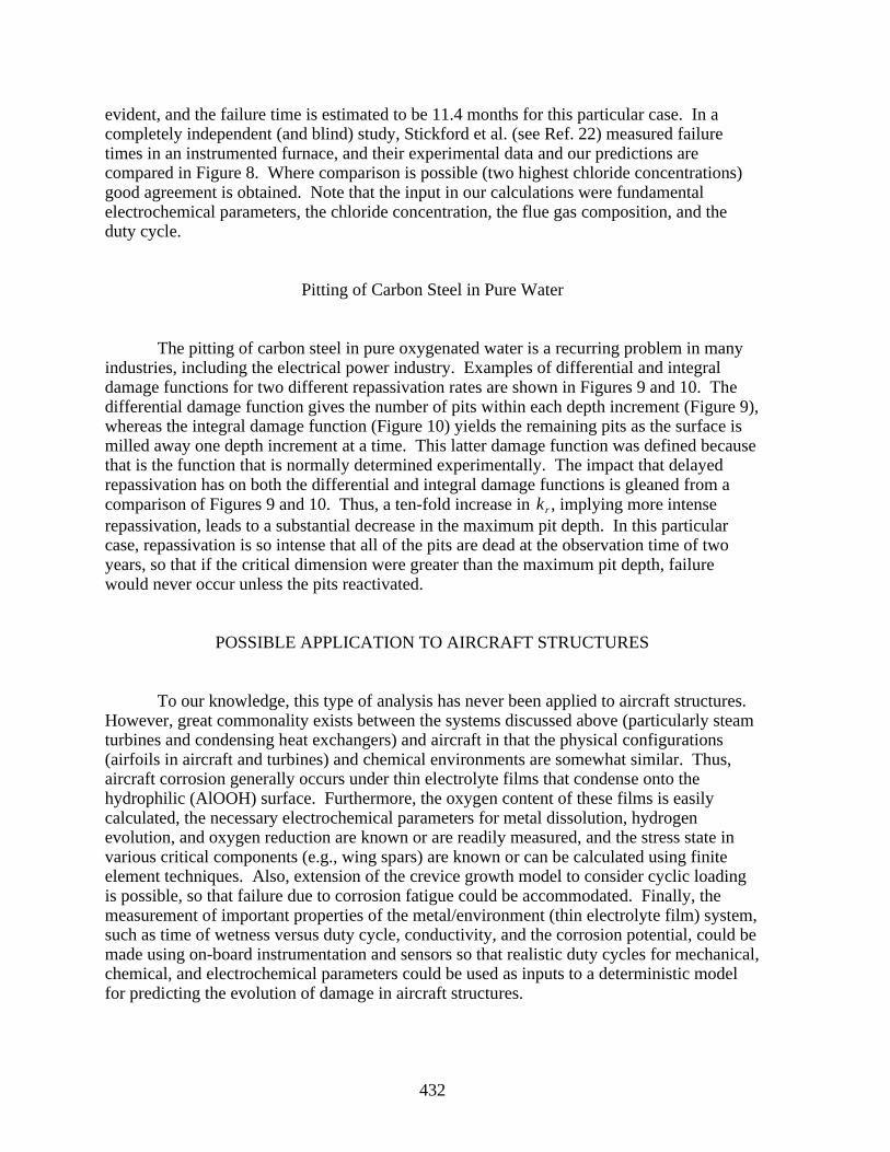
432
evident, and the failure time is estimated to be 11.4 months for this particular case. In acompletely independent (and blind) study, Stickford et al. (see Ref. 22) measured failuretimes in an instrumented furnace, and their experimental data and our predictions arecompared in Figure 8. Where comparison is possible (two highest chloride concentrations)good agreement is obtained. Note that the input in our calculations were fundamentalelectrochemical parameters, the chloride concentration, the flue gas composition, and theduty cycle.
Pitting of Carbon Steel in Pure Water
The pitting of carbon steel in pure oxygenated water is a recurring problem in manyindustries, including the electrical power industry. Examples of differential and integraldamage functions for two different repassivation rates are shown in Figures 9 and 10. Thedifferential damage function gives the number of pits within each depth increment (Figure 9),whereas the integral damage function (Figure 10) yields the remaining pits as the surface ismilled away one depth increment at a time. This latter damage function was defined becausethat is the function that is normally determined experimentally. The impact that delayedrepassivation has on both the differential and integral damage functions is gleaned from acomparison of Figures 9 and 10. Thus, a ten-fold increase in kr , implying more intenserepassivation, leads to a substantial decrease in the maximum pit depth. In this particularcase, repassivation is so intense that all of the pits are dead at the observation time of twoyears, so that if the critical dimension were greater than the maximum pit depth, failurewould never occur unless the pits reactivated.
POSSIBLE APPLICATION TO AIRCRAFT STRUCTURES
To our knowledge, this type of analysis has never been applied to aircraft structures.However, great commonality exists between the systems discussed above (particularly steamturbines and condensing heat exchangers) and aircraft in that the physical configurations(airfoils in aircraft and turbines) and chemical environments are somewhat similar. Thus,aircraft corrosion generally occurs under thin electrolyte films that condense onto thehydrophilic (AlOOH) surface. Furthermore, the oxygen content of these films is easilycalculated, the necessary electrochemical parameters for metal dissolution, hydrogenevolution, and oxygen reduction are known or are readily measured, and the stress state invarious critical components (e.g., wing spars) are known or can be calculated using finiteelement techniques. Also, extension of the crevice growth model to consider cyclic loadingis possible, so that failure due to corrosion fatigue could be accommodated. Finally, themeasurement of important properties of the metal/environment (thin electrolyte film) system,such as time of wetness versus duty cycle, conductivity, and the corrosion potential, could bemade using on-board instrumentation and sensors so that realistic duty cycles for mechanical,chemical, and electrochemical parameters could be used as inputs to a deterministic modelfor predicting the evolution of damage in aircraft structures.

433
ACKNOWLEDGMENTS
The authors gratefully acknowledge the support of this work by the US Departmentof Energy/Basic Energy Sciences under Grant No. DE-DG03-84ER45164.
REFERENCES
1. Macdonald, D. D. and Urquidi-Macdonald, M.: Corrosion, vol. 48, no. 5, 1992, p. 354.
2. Lin, L. F., Chao, C. Y., and Macdonald, D. D.: J. Electrochem. Soc., vol. 128, 1981,p. 1194.
3. Macdonald, D. D. and Urquidi-Macdonald, M.: Electrochem. Acta, vol. 31, 1986,p. 1079.
4. Macdonald, D. D. and Urquidi-Macdonald, M.: J. Electrochem. Soc., vol. 134, 1987,p. 41.
5. Macdonald, D. D. and Urquidi-Macdonald, M.: J. Electrochem. Soc., vol. 136, 1989,p. 961.
6. Macdonald, D. D.: J. Electrochem. Soc., vol. 139, 1992, p. 3434.
7. Macdonald, D. D. and Urquidi-Macdonald, M.: Corros. Sci., vol. 32, 1991, p. 51.
8. Macdonald, D. D. and Urquidi-Macdonald, M.: Proc. 5th Intl. Symp. Environ.Degrad. Mat. in Nucl. Power Systs.--Water Reactors, ANS, LaGrange Park, IL, 1992,p. 345.
9. Macdonald, D. D. and Urquidi-Macdonald, M.: CORROSION/92, paper no. 87,Houston, TX.
10. Macdonald, D. D., Urquidi-Macdonald, M., and Lu, P.-C.: CORROSION/94, paperno. 246, Baltimore, MD.
11. Lu, P.-C.: Ph.D. Dissertation, The Pennsylvania State University, 1994.
12. Macdonald, D. D. and Yeh, T.-K.: Nucl. Sci. Eng., vol. 121, 1995, p. 468.
13. Yeh, T.-K.: Ph.D. Dissertation, The Pennsylvania State University, 1994.
14. Pistorius, P. C. and Burstein, G. T.: Phil. Trans. R. Soc. London A., vol. 341, 1992,p. 531.
15. Frankel, G. S., Stockert, L., Hunkeler, F., and Bohni, H.: Corros. Sci., vol. 43, 1987,p. 429.
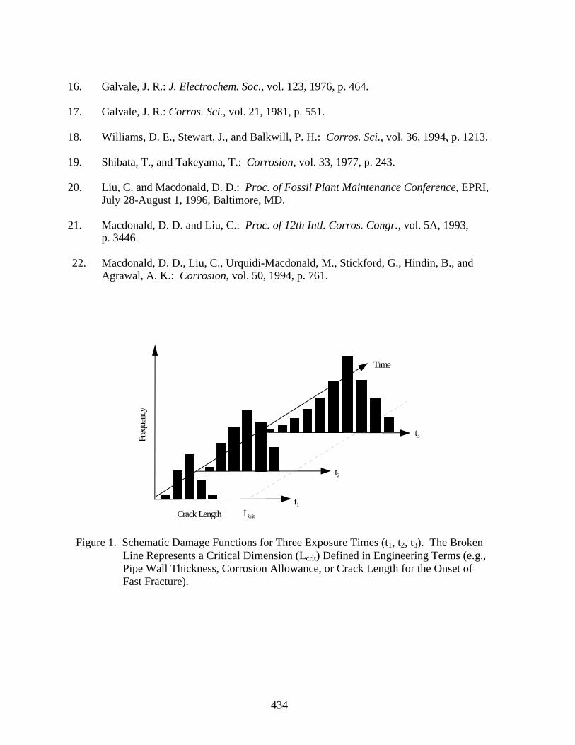
434
16. Galvale, J. R.: J. Electrochem. Soc., vol. 123, 1976, p. 464.
17. Galvale, J. R.: Corros. Sci., vol. 21, 1981, p. 551.
18. Williams, D. E., Stewart, J., and Balkwill, P. H.: Corros. Sci., vol. 36, 1994, p. 1213.
19. Shibata, T., and Takeyama, T.: Corrosion, vol. 33, 1977, p. 243.
20. Liu, C. and Macdonald, D. D.: Proc. of Fossil Plant Maintenance Conference, EPRI,July 28-August 1, 1996, Baltimore, MD.
21. Macdonald, D. D. and Liu, C.: Proc. of 12th Intl. Corros. Congr., vol. 5A, 1993,p. 3446.
22. Macdonald, D. D., Liu, C., Urquidi-Macdonald, M., Stickford, G., Hindin, B., andAgrawal, A. K.: Corrosion, vol. 50, 1994, p. 761.
Freq
uenc
y
Crack Length Lcrit
Time
t1
t2
t3
Figure 1. Schematic Damage Functions for Three Exposure Times (t1, t2, t3). The BrokenLine Represents a Critical Dimension (Lcrit) Defined in Engineering Terms (e.g.,Pipe Wall Thickness, Corrosion Allowance, or Crack Length for the Onset ofFast Fracture).
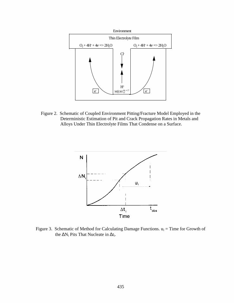
435
e- e-M OH( )n
z−n( )+
Cl-
H+
Environment
Thin Electrolyte Film
O2 + 4H+ + 4e- => 2H2O O2 + 4H+ + 4e- => 2H2O
Figure 2. Schematic of Coupled Environment Pitting/Fracture Model Employed in theDeterministic Estimation of Pit and Crack Propagation Rates in Metals andAlloys Under Thin Electrolyte Films That Condense on a Surface.
Figure 3. Schematic of Method for Calculating Damage Functions. ui = Time for Growth ofthe ∆Ni Pits That Nucleate in ∆ti.
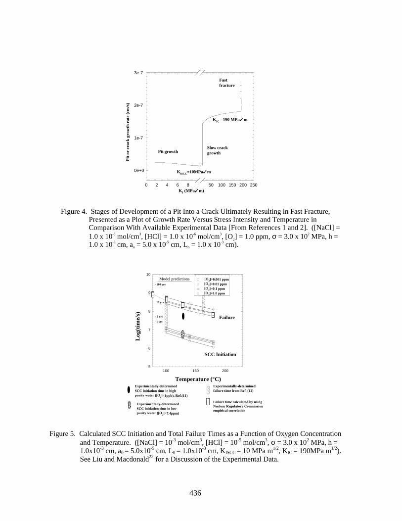
436
0 2 4 6 8 50 100 150 200 250
0e+0
1e-7
2e-7
3e-7
KISCC=10MPa m
K IC =190 MPa m
Fastfracture
K I (MPa m)
Pit growth growthSlow crack
Pit
or c
rack
gro
wth
rat
e (c
m/s
)
Figure 4. Stages of Development of a Pit Into a Crack Ultimately Resulting in Fast Fracture,Presented as a Plot of Growth Rate Versus Stress Intensity and Temperature inComparison With Available Experimental Data [From References 1 and 2]. ([NaCl] =1.0 x 10⁻³ mol/cm3, [HCl] = 1.0 x 10⁻⁶ mol/cm3, [O2] = 1.0 ppm, σ = 3.0 x 10² MPa, h =1.0 x 10⁻³ cm, a0 = 5.0 x 10⁻⁵ cm, L0 = 1.0 x 10⁻³ cm).
purity water ([O 2]=7.4ppm)SCC initiation time in low Experimentally-determined
purity water ([O 2]<1ppb), Ref.(11)SCC initiation time in high Experimentally-determined
Failure time calculated by usingNuclear Regulatory Commissionempirical correlation
failure time from Ref. (12)Experimentally-determined
100 150 2005
6
7
8
9
10
SCC Initiation
Failure
Temperature (°C)
Log(
time/
s)
- 100 yrs
[O2]=1.0 ppm[O2]=0.1 ppm
[O2]=0.001 ppm[O2]=0.01 ppm
- 2 yrs
10 yrs
- 1 yrs
Model predictions
Figure 5. Calculated SCC Initiation and Total Failure Times as a Function of Oxygen Concentrationand Temperature. ([NaCl] = 10-3 mol/cm3, [HCl] = 10-5 mol/cm3, σ = 3.0 x 10² MPa, h =1.0x10⁻³ cm, a0 = 5.0x10⁻⁵ cm, L0 = 1.0x10⁻³ cm, KISCC = 10 MPa m1/2, KIC = 190MPa m1/2).See Liu and Macdonald22 for a Discussion of the Experimental Data.
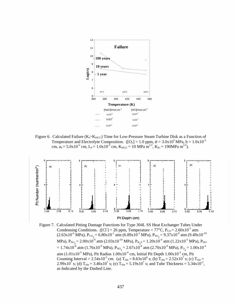
437
Log(
t/s)
360 380 400 420 440 4605
6
7
8
9
10
11
12
- 1 year
10 years
- 100 years
Failure
Temperature (K)
180oC140oC97oC
[NaCl]/mol.cm-3 [HCl]/mol.cm-3
1x10⁻⁸ 1x10⁻⁸
1x10-71x10-7
1x10⁻³ 1x10⁻³
Figure 6. Calculated Failure (KI>KISCC) Time for Low-Pressure Steam Turbine Disk as a Function ofTemperature and Electrolyte Composition. ([O2] = 1.0 ppm, σ = 3.0x10² MPa, h = 1.0x10⁻³
cm, a0 = 5.0x10⁻⁵ cm, L0 = 1.0x10⁻³ cm, KISCC = 10 MPa m1/2, KIC = 190MPa m1/2).
Figure 7. Calculated Pitting Damage Functions for Type 304L SS Heat Exchanger Tubes UnderCondensing Conditions. ([Cl-] = 26 ppm, Temperature = 77°C, PCO = 2.60x10⁻⁵ atm(2.63x10⁻⁶ MPa), PCO
2 = 6.80x10⁻² atm (6.89x10⁻³ MPa), PSO
2 = 9.37x10⁻⁹ atm (9.49x10⁻¹⁰
MPa), PSO3 = 2.00x10⁻⁹ atm (2.03x10⁻¹⁰ MPa), PH
2S = 1.20x10⁻⁴ atm (1.22x10⁻⁵ MPa), PNO
= 1.74x10⁻⁸ atm (1.76x10⁻⁹ MPa), PNO2 = 2.67x10⁻⁸ atm (2.70x10⁻⁹ MPa), PO
2 = 1.00x10⁻⁴
atm (1.01x10⁻⁵ MPa), Pit Radius 1.00x10⁻⁴ cm, Initial Pit Depth 1.00x10⁻³ cm, PitCounting Interval = 2.54x10⁻³ cm. (a) Tobs = 8.63x10⁶ s; (b) Tobs = 2.52x10⁷ s; (c) Tobs =2.99x10⁷ s; (d) Tobs = 3.46x10⁷ s; (e) Tobs = 5.19x10⁷ s; and Tube Thickness = 5.34x10⁻²,as Indicated by the Dashed Line.
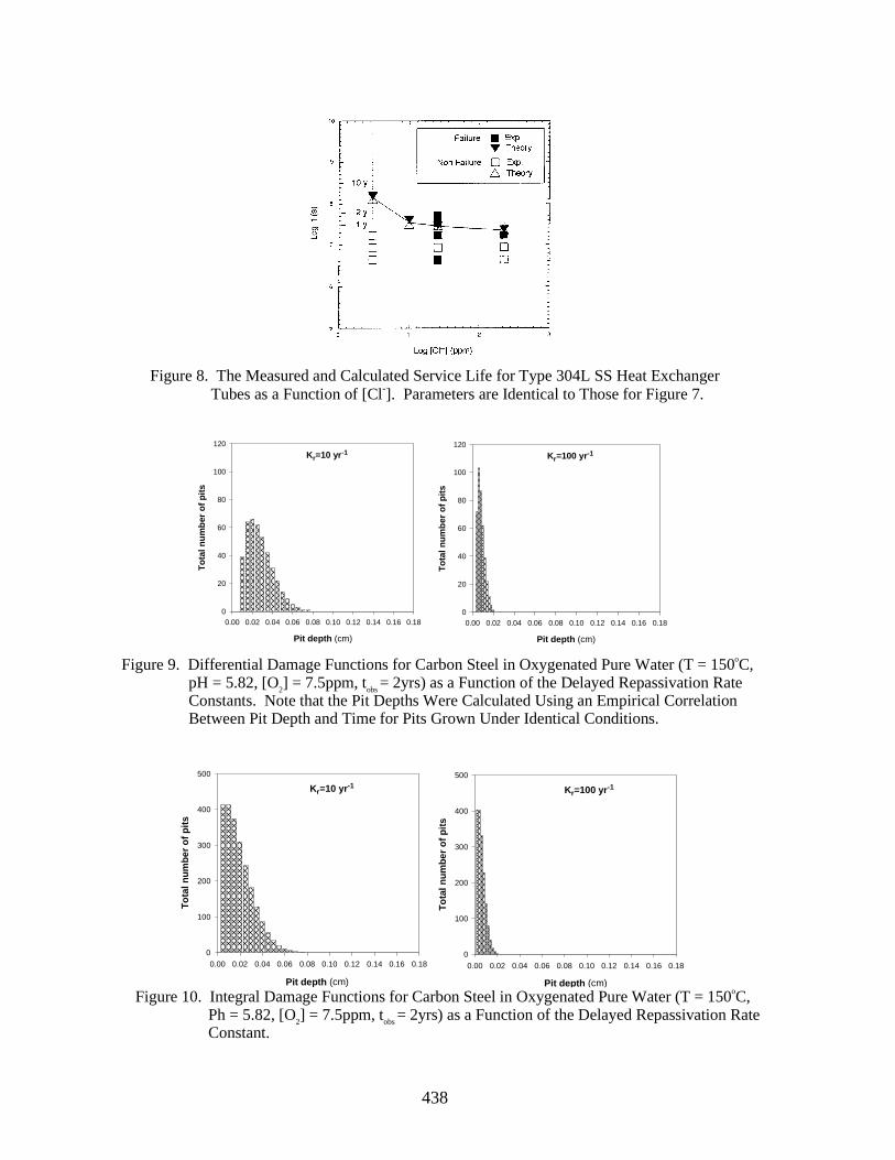
438
Figure 8. The Measured and Calculated Service Life for Type 304L SS Heat ExchangerTubes as a Function of [Cl-]. Parameters are Identical to Those for Figure 7.
Kr=10 yr -1
Pit depth (cm)
0.00 0.02 0.04 0.06 0.08 0.10 0.12 0.14 0.16 0.18
Tot
al n
umbe
r of
pits
0
20
40
60
80
100
120
Kr=100 yr-1
Pit depth (cm)
0.00 0.02 0.04 0.06 0.08 0.10 0.12 0.14 0.16 0.18
Tot
al n
umbe
r of
pits
0
20
40
60
80
100
120
Kr=10 yr -1
Pit depth (cm)
0.00 0.02 0.04 0.06 0.08 0.10 0.12 0.14 0.16 0.18
Tot
al n
umbe
r of
pits
0
100
200
300
400
500
Kr=100 yr -1
Pit depth (cm)
0.00 0.02 0.04 0.06 0.08 0.10 0.12 0.14 0.16 0.18
Tot
al n
umbe
r of
pits
0
100
200
300
400
500
Figure 10. Integral Damage Functions for Carbon Steel in Oxygenated Pure Water (T = 150oC,Ph = 5.82, [O2] = 7.5ppm, tobs = 2yrs) as a Function of the Delayed Repassivation RateConstant.
Figure 9. Differential Damage Functions for Carbon Steel in Oxygenated Pure Water (T = 150oC,pH = 5.82, [O2] = 7.5ppm, tobs = 2yrs) as a Function of the Delayed Repassivation RateConstants. Note that the Pit Depths Were Calculated Using an Empirical CorrelationBetween Pit Depth and Time for Pits Grown Under Identical Conditions.
439
INVESTIGATION OF FUSELAGE STRUCTURE SUBJECT TOWIDESPREAD FATIGUE DAMAGE
M. L. Gruber, K. E. Wilkins, and R. E. WordenThe Boeing Company
Seattle, WA
ABSTRACT
This paper presents work sponsored by the Federal Aviation Administration (FAA)under a contract titled “Investigation of Fuselage Structure Subject to Widespread FatigueDamage.” Two generic wide-body fuselage panels containing cracks in the upper rivet row ofa lap joint were tested to obtain crack growth rate and residual strength data with and withoutthe presence of simulated multiple site damage. Also, finite element models were used topredict the crack growth history of the lead cracks and the residual strength of the panels. Inaddition to the FAA contract results, this paper discusses independent work to evaluateavailable analysis methods and to develop an engineering analysis tool for predicting the effectof multiple site damage on residual strength.
INTRODUCTION
High replacement costs and competition have led airline operators to use theirairplanes beyond the original design service objective. The result is an aging fleet with ahigher probability of fatigue-initiated cracking and eventually widespread fatigue damage(WFD). WFD is defined as the simultaneous presence of cracks at multiple structural detailsthat are of sufficient size and density whereby the structure no longer meets its damagetolerance requirements. A subset of WFD is multiple site damage (MSD), which ischaracterized by the simultaneous presence of fatigue cracks in the same structural element.Damage tolerance analysis methods that focus primarily on local damage may not be sufficientto account for the effects of WFD. It is possible that small undetected MSD in adjacentfastener holes might link together and increase the rate of damage growth in a lap joint. Thisscenario would reduce the opportunities to find the damage prior to failure. Furthermore, theresidual strength may be impacted and the final critical damage size may be smaller in thepresence of MSD. Finally, crack arrest devices such as tear straps may not be as effective asoriginally designed.
An increased understanding of MSD behavior would allow the aging fleet to beevaluated on a model-by-model basis once proven analytical methods are available.Modifications could be made to susceptible structure as required. For new configurations, an
440
understanding of the fundamental behavior of MSD would allow engineers to developstructural designs capable of containing MSD.
This paper includes recent work performed under the FAA contract titled“Investigation of Fuselage Structure Subject to Widespread Fatigue Damage” (ref. 1) andongoing work at Boeing to investigate the behavior of airplane fuselage structure containingMSD.
WFD CONTRACT RESULTS
The primary program objective was to obtain data on airplane fuselage structuresubject to MSD in an environment that reflects typical commercial jetliner manufacturing andoperating conditions. The program involved both full-scale testing and analysis of pressurizedstiffened panel structure. Testing was performed on two generic wide-body fuselage panelscontaining frame centered cracks in the outer skin of a lap joint along the upper row of rivets.Crack growth and residual strength were measured on panels with and without simulatedMSD. Finite element models of the test panels containing skin cracks were analyzed. Stressintensity factors calculated from the finite element analyses were used to predict the residualstrength of the panels and the crack growth rate of the lead crack. The results of these tasksare summarized in the following sections.
MATERIAL PROPERTY TESTS
Stress-strain, crack growth rate, and fracture toughness properties were developed for0.063-inch-thick clad 2024-T3 aluminum using specimens fabricated from the same lot ofmaterial used to fabricate the large curved pressure panels. These properties were developedfor the transverse material orientation, corresponding to the typical material orientation forhoop loading in a fuselage skin panel and used in the large curved pressure panel analysis.Four center-cracked tension M(t) panels were used to develop crack growth, R-curve, andtoughness properties, while two tensile specimens were used to develop stress-strain data.The results are shown in table 1.
Table 1. 2024-T3 Transverse Material Properties.
Tensile Modulus
(Msi)
Tensile Yield
0.2% (ksi)
Tensile Ultimate
(ksi)
Kapparent
(ksi in1/2
9.86 42.8 64.3 130
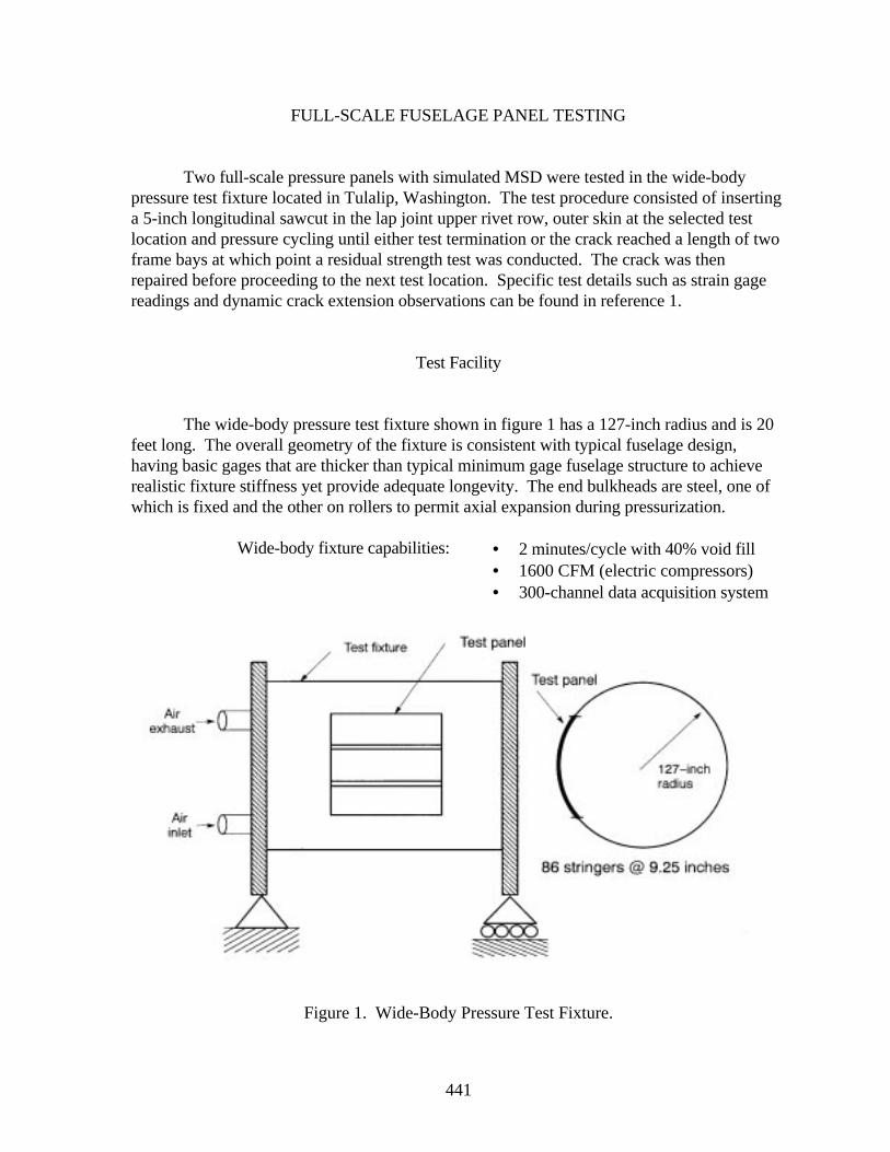
441
FULL-SCALE FUSELAGE PANEL TESTING
Two full-scale pressure panels with simulated MSD were tested in the wide-bodypressure test fixture located in Tulalip, Washington. The test procedure consisted of insertinga 5-inch longitudinal sawcut in the lap joint upper rivet row, outer skin at the selected testlocation and pressure cycling until either test termination or the crack reached a length of twoframe bays at which point a residual strength test was conducted. The crack was thenrepaired before proceeding to the next test location. Specific test details such as strain gagereadings and dynamic crack extension observations can be found in reference 1.
Test Facility
The wide-body pressure test fixture shown in figure 1 has a 127-inch radius and is 20feet long. The overall geometry of the fixture is consistent with typical fuselage design,having basic gages that are thicker than typical minimum gage fuselage structure to achieverealistic fixture stiffness yet provide adequate longevity. The end bulkheads are steel, one ofwhich is fixed and the other on rollers to permit axial expansion during pressurization.
Wide-body fixture capabilities: • 2 minutes/cycle with 40% void fill• 1600 CFM (electric compressors)• 300-channel data acquisition system
Figure 1. Wide-Body Pressure Test Fixture.
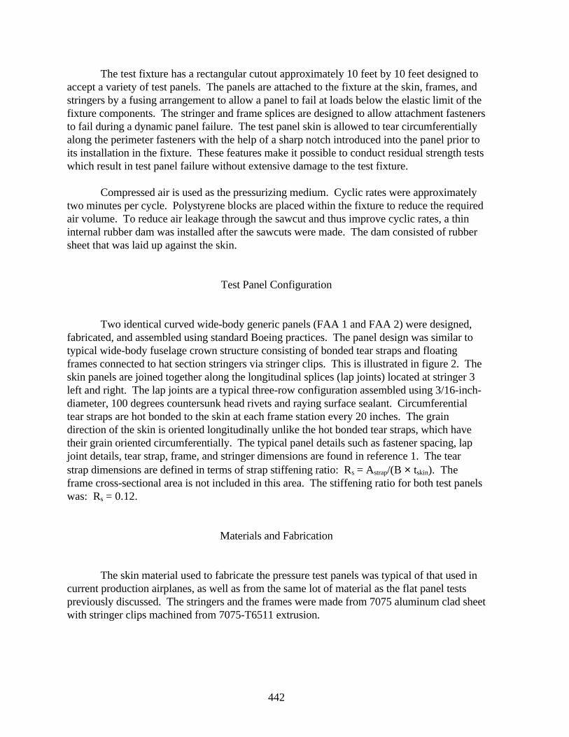
442
The test fixture has a rectangular cutout approximately 10 feet by 10 feet designed toaccept a variety of test panels. The panels are attached to the fixture at the skin, frames, andstringers by a fusing arrangement to allow a panel to fail at loads below the elastic limit of thefixture components. The stringer and frame splices are designed to allow attachment fastenersto fail during a dynamic panel failure. The test panel skin is allowed to tear circumferentiallyalong the perimeter fasteners with the help of a sharp notch introduced into the panel prior toits installation in the fixture. These features make it possible to conduct residual strength testswhich result in test panel failure without extensive damage to the test fixture.
Compressed air is used as the pressurizing medium. Cyclic rates were approximatelytwo minutes per cycle. Polystyrene blocks are placed within the fixture to reduce the requiredair volume. To reduce air leakage through the sawcut and thus improve cyclic rates, a thininternal rubber dam was installed after the sawcuts were made. The dam consisted of rubbersheet that was laid up against the skin.
Test Panel Configuration
Two identical curved wide-body generic panels (FAA 1 and FAA 2) were designed,fabricated, and assembled using standard Boeing practices. The panel design was similar totypical wide-body fuselage crown structure consisting of bonded tear straps and floatingframes connected to hat section stringers via stringer clips. This is illustrated in figure 2. Theskin panels are joined together along the longitudinal splices (lap joints) located at stringer 3left and right. The lap joints are a typical three-row configuration assembled using 3/16-inch-diameter, 100 degrees countersunk head rivets and raying surface sealant. Circumferentialtear straps are hot bonded to the skin at each frame station every 20 inches. The graindirection of the skin is oriented longitudinally unlike the hot bonded tear straps, which havetheir grain oriented circumferentially. The typical panel details such as fastener spacing, lapjoint details, tear strap, frame, and stringer dimensions are found in reference 1. The tearstrap dimensions are defined in terms of strap stiffening ratio: Rs = Astrap/(B × tskin). Theframe cross-sectional area is not included in this area. The stiffening ratio for both test panelswas: Rs = 0.12.
Materials and Fabrication
The skin material used to fabricate the pressure test panels was typical of that used incurrent production airplanes, as well as from the same lot of material as the flat panel testspreviously discussed. The stringers and the frames were made from 7075 aluminum clad sheetwith stringer clips machined from 7075-T6511 extrusion.
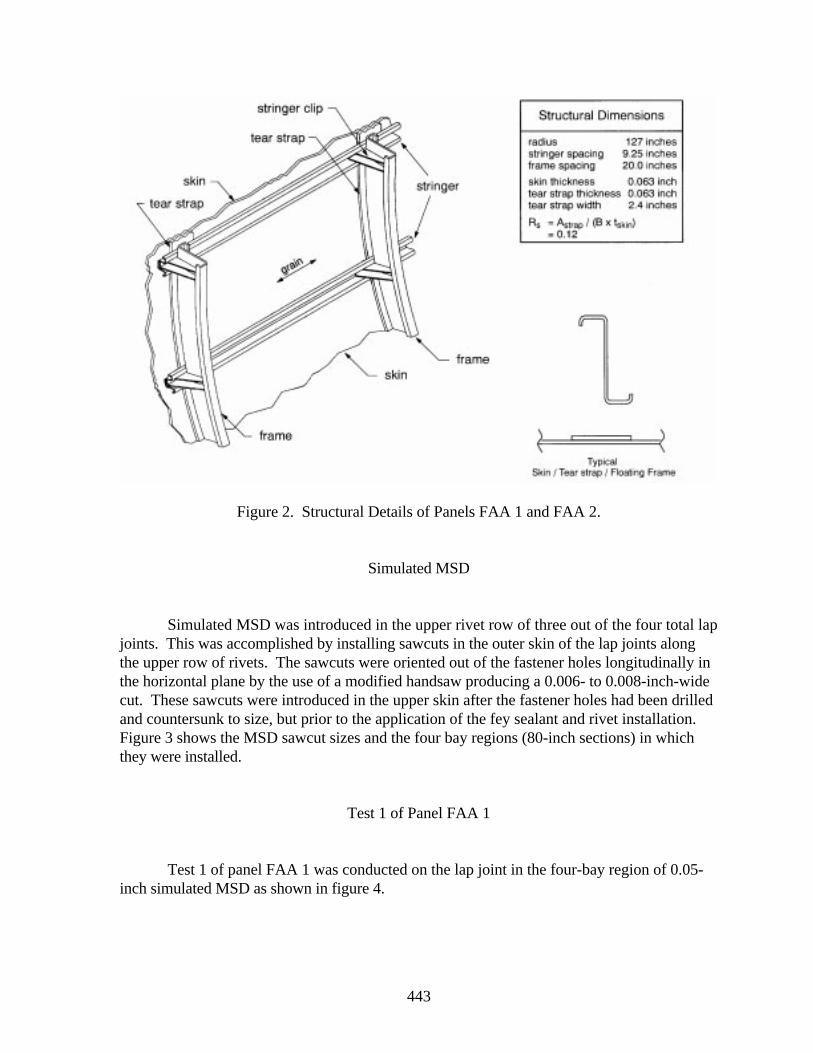
443
Figure 2. Structural Details of Panels FAA 1 and FAA 2.
Simulated MSD
Simulated MSD was introduced in the upper rivet row of three out of the four total lapjoints. This was accomplished by installing sawcuts in the outer skin of the lap joints alongthe upper row of rivets. The sawcuts were oriented out of the fastener holes longitudinally inthe horizontal plane by the use of a modified handsaw producing a 0.006- to 0.008-inch-widecut. These sawcuts were introduced in the upper skin after the fastener holes had been drilledand countersunk to size, but prior to the application of the fey sealant and rivet installation.Figure 3 shows the MSD sawcut sizes and the four bay regions (80-inch sections) in whichthey were installed.
Test 1 of Panel FAA 1
Test 1 of panel FAA 1 was conducted on the lap joint in the four-bay region of 0.05-inch simulated MSD as shown in figure 4.
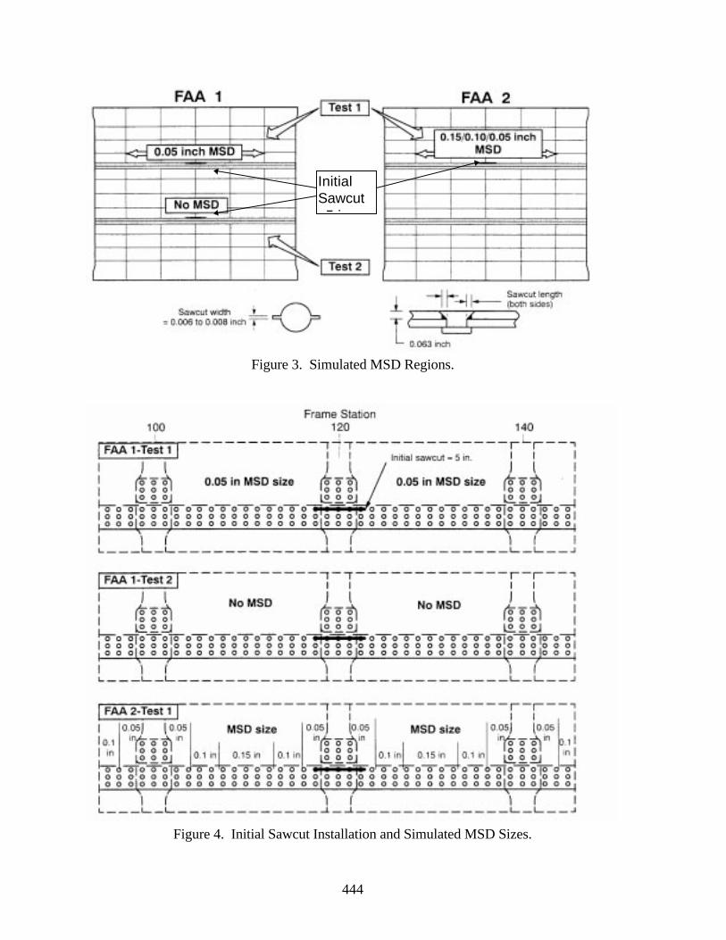
444
Figure 3. Simulated MSD Regions.
Figure 4. Initial Sawcut Installation and Simulated MSD Sizes.
InitialSawcut5 i

445
A 5-inch sawcut was installed in the outer skin only, centered at frame station 120.The panel was pressure cycled at 8.6 psi. No crack initiations were visible after 281 pressurecycles. At that point the station 120 tear strap bridging the sawcut was cut. As cyclingcontinued, the main crack steadily grew to approximately 6.5 inches, at which point the 0.05-inch MSD sawcuts one fastener ahead of the tips of the main crack had grown from under therivets and had become visible.
The main crack extended dynamically at 1233 cycles after reaching a length of 17.2inches and arrested at a length of 37.4 inches. The tear straps contained the dynamic crack,but visible cracks did develop in the fasteners common to the tear straps at the next adjacentframes, stations 100 and 140 respectively.
No residual strength test was conducted at this test location due to the potentialdestruction of the entire test panel prior to conducting Test 2 (the only non-MSD test in theprogram), which was intended to be used as the basis for measuring the influence of MSD onresidual strength. The test location was repaired by applying a small external doubler over thecrack.
Test 2 of Panel FAA 1
Test 2 of panel FAA 1 was conducted on the lap joint with no MSD, as shown infigure 4.
A 5-inch sawcut was then installed in the outer skin and tear strap centered on framestation 120. The panel was pressure cycled at 8.6 psi. After 1172 pressure cycles, no crackgrowth had been detected from the sawcut, and thus the sawcut was extended to 5.72 inches,terminating approximately 0.25 inch beyond a fastener hole at each end of the sawcut. Ascycling continued the main crack steadily grew to a length of 36.91 inches.
The residual strength test of FAA 1-Test 2 consisted of increasing the internal pressurein small intervals until dynamic panel failure occurred. Prior to running the residual strengthtest the central frame at station 120 was severed. The crack length prior to pressurizing was36.91 inches with the crack tips adjacent to the edges of the tear straps. As the pressure wasincreased the crack stably grew to a length of approximately 38.2 inches where, at a pressureof 9.4 psi, the crack ran dynamically to the ends of the panel, resulting in catastrophic failure.The configuration prior to failure is shown in figure 5.
Test 1 of Panel FAA 2
Test 1 of panel FAA-2 was conducted on the upper row of the lap joint in the four-bayregion of variable size (0.05, 0.10 and 0.15 inch) simulated MSD, as shown in figure 4.
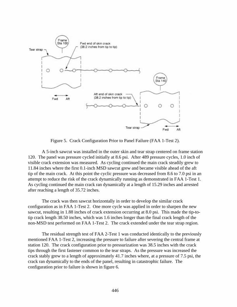
446
Figure 5. Crack Configuration Prior to Panel Failure (FAA 1-Test 2).
A 5-inch sawcut was installed in the outer skin and tear strap centered on frame station120. The panel was pressure cycled initially at 8.6 psi. After 489 pressure cycles, 1.0 inch ofvisible crack extension was measured. As cycling continued the main crack steadily grew to11.84 inches where the first 0.1-inch MSD sawcut grew and became visible ahead of the afttip of the main crack. At this point the cyclic pressure was decreased from 8.6 to 7.0 psi in anattempt to reduce the risk of the crack dynamically running as demonstrated in FAA 1-Test 1.As cycling continued the main crack ran dynamically at a length of 15.29 inches and arrestedafter reaching a length of 35.72 inches.
The crack was then sawcut horizontally in order to develop the similar crackconfiguration as in FAA 1-Test 2. One more cycle was applied in order to sharpen the newsawcut, resulting in 1.88 inches of crack extension occurring at 8.0 psi. This made the tip-to-tip crack length 38.50 inches, which was 1.6 inches longer than the final crack length of thenon-MSD test performed on FAA 1-Test 2. The crack extended under the tear strap region.
The residual strength test of FAA 2-Test 1 was conducted identically to the previouslymentioned FAA 1-Test 2, increasing the pressure to failure after severing the central frame atstation 120. The crack configuration prior to pressurization was 38.5 inches with the cracktips through the first fastener common to the tear straps. As the pressure was increased thecrack stably grew to a length of approximately 41.7 inches where, at a pressure of 7.5 psi, thecrack ran dynamically to the ends of the panel, resulting in catastrophic failure. Theconfiguration prior to failure is shown in figure 6.
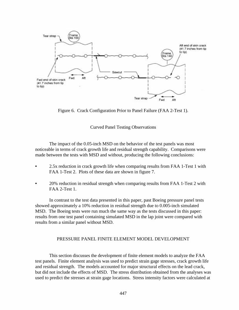
447
Figure 6. Crack Configuration Prior to Panel Failure (FAA 2-Test 1).
Curved Panel Testing Observations
The impact of the 0.05-inch MSD on the behavior of the test panels was mostnoticeable in terms of crack growth life and residual strength capability. Comparisons weremade between the tests with MSD and without, producing the following conclusions:
• 2.5x reduction in crack growth life when comparing results from FAA 1-Test 1 withFAA 1-Test 2. Plots of these data are shown in figure 7.
• 20% reduction in residual strength when comparing results from FAA 1-Test 2 with
FAA 2-Test 1.
In contrast to the test data presented in this paper, past Boeing pressure panel testsshowed approximately a 10% reduction in residual strength due to 0.005-inch simulatedMSD. The Boeing tests were run much the same way as the tests discussed in this paper:results from one test panel containing simulated MSD in the lap joint were compared withresults from a similar panel without MSD.
PRESSURE PANEL FINITE ELEMENT MODEL DEVELOPMENT
This section discusses the development of finite element models to analyze the FAAtest panels. Finite element analysis was used to predict strain gage stresses, crack growth lifeand residual strength. The models accounted for major structural effects on the lead crack,but did not include the effects of MSD. The stress distribution obtained from the analyses wasused to predict the stresses at strain gage locations. Stress intensity factors were calculated at
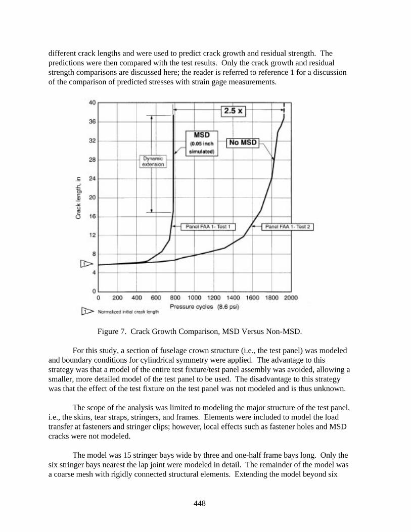
448
different crack lengths and were used to predict crack growth and residual strength. Thepredictions were then compared with the test results. Only the crack growth and residualstrength comparisons are discussed here; the reader is referred to reference 1 for a discussionof the comparison of predicted stresses with strain gage measurements.
Figure 7. Crack Growth Comparison, MSD Versus Non-MSD.
For this study, a section of fuselage crown structure (i.e., the test panel) was modeledand boundary conditions for cylindrical symmetry were applied. The advantage to thisstrategy was that a model of the entire test fixture/test panel assembly was avoided, allowing asmaller, more detailed model of the test panel to be used. The disadvantage to this strategywas that the effect of the test fixture on the test panel was not modeled and is thus unknown.
The scope of the analysis was limited to modeling the major structure of the test panel,i.e., the skins, tear straps, stringers, and frames. Elements were included to model the loadtransfer at fasteners and stringer clips; however, local effects such as fastener holes and MSDcracks were not modeled.
The model was 15 stringer bays wide by three and one-half frame bays long. Only thesix stringer bays nearest the lap joint were modeled in detail. The remainder of the model wasa coarse mesh with rigidly connected structural elements. Extending the model beyond six
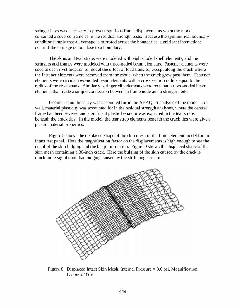
449
stringer bays was necessary to prevent spurious frame displacements when the modelcontained a severed frame as in the residual strength tests. Because the symmetrical boundaryconditions imply that all damage is mirrored across the boundaries, significant interactionsoccur if the damage is too close to a boundary.
The skins and tear straps were modeled with eight-noded shell elements, and thestringers and frames were modeled with three-noded beam elements. Fastener elements wereused at each rivet location to model the effect of load transfer, except along the crack wherethe fastener elements were removed from the model when the crack grew past them. Fastenerelements were circular two-noded beam elements with a cross section radius equal to theradius of the rivet shank. Similarly, stringer clip elements were rectangular two-noded beamelements that made a simple connection between a frame node and a stringer node.
Geometric nonlinearity was accounted for in the ABAQUS analysis of the model. Aswell, material plasticity was accounted for in the residual strength analyses, where the centralframe had been severed and significant plastic behavior was expected in the tear strapsbeneath the crack tips. In the model, the tear strap elements beneath the crack tips were givenplastic material properties.
Figure 8 shows the displaced shape of the skin mesh of the finite element model for anintact test panel. Here the magnification factor on the displacements is high enough to see thedetail of the skin bulging and the lap joint rotation. Figure 9 shows the displaced shape of theskin mesh containing a 30-inch crack. Here the bulging of the skin caused by the crack ismuch more significant than bulging caused by the stiffening structure.
Figure 8. Displaced Intact Skin Mesh, Internal Pressure = 8.6 psi, MagnificationFactor ≈ 100x.
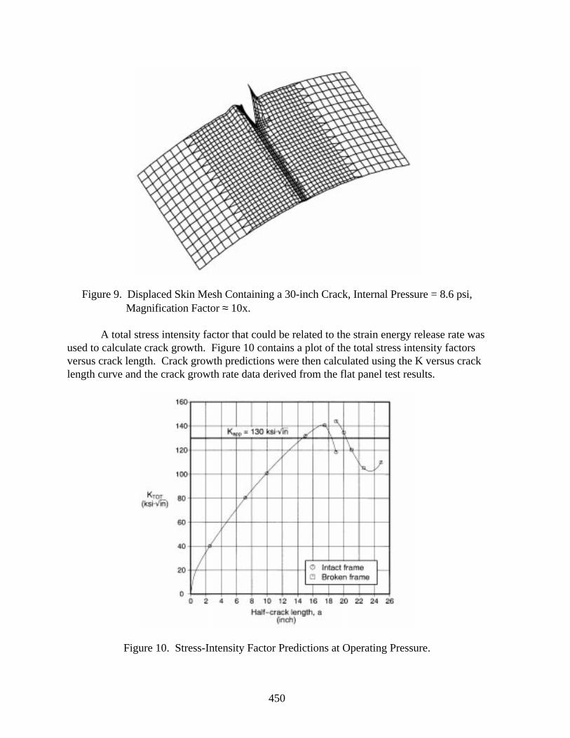
450
Figure 9. Displaced Skin Mesh Containing a 30-inch Crack, Internal Pressure = 8.6 psi,Magnification Factor ≈ 10x.
A total stress intensity factor that could be related to the strain energy release rate wasused to calculate crack growth. Figure 10 contains a plot of the total stress intensity factorsversus crack length. Crack growth predictions were then calculated using the K versus cracklength curve and the crack growth rate data derived from the flat panel test results.
Figure 10. Stress-Intensity Factor Predictions at Operating Pressure.
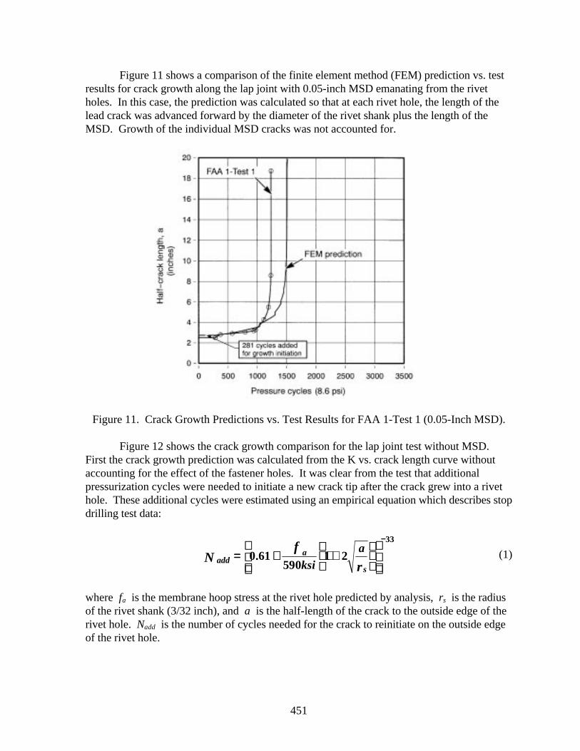
451
Figure 11 shows a comparison of the finite element method (FEM) prediction vs. testresults for crack growth along the lap joint with 0.05-inch MSD emanating from the rivetholes. In this case, the prediction was calculated so that at each rivet hole, the length of thelead crack was advanced forward by the diameter of the rivet shank plus the length of theMSD. Growth of the individual MSD cracks was not accounted for.
Figure 11. Crack Growth Predictions vs. Test Results for FAA 1-Test 1 (0.05-Inch MSD).
Figure 12 shows the crack growth comparison for the lap joint test without MSD.First the crack growth prediction was calculated from the K vs. crack length curve withoutaccounting for the effect of the fastener holes. It was clear from the test that additionalpressurization cycles were needed to initiate a new crack tip after the crack grew into a rivethole. These additional cycles were estimated using an empirical equation which describes stopdrilling test data:
adda
sN
f
rksia== ++ ++
−−
0 61590
1 2
33
. (1)
where fa is the membrane hoop stress at the rivet hole predicted by analysis, rs is the radiusof the rivet shank (3/32 inch), and a is the half-length of the crack to the outside edge of therivet hole. Nadd is the number of cycles needed for the crack to reinitiate on the outside edgeof the rivet hole.
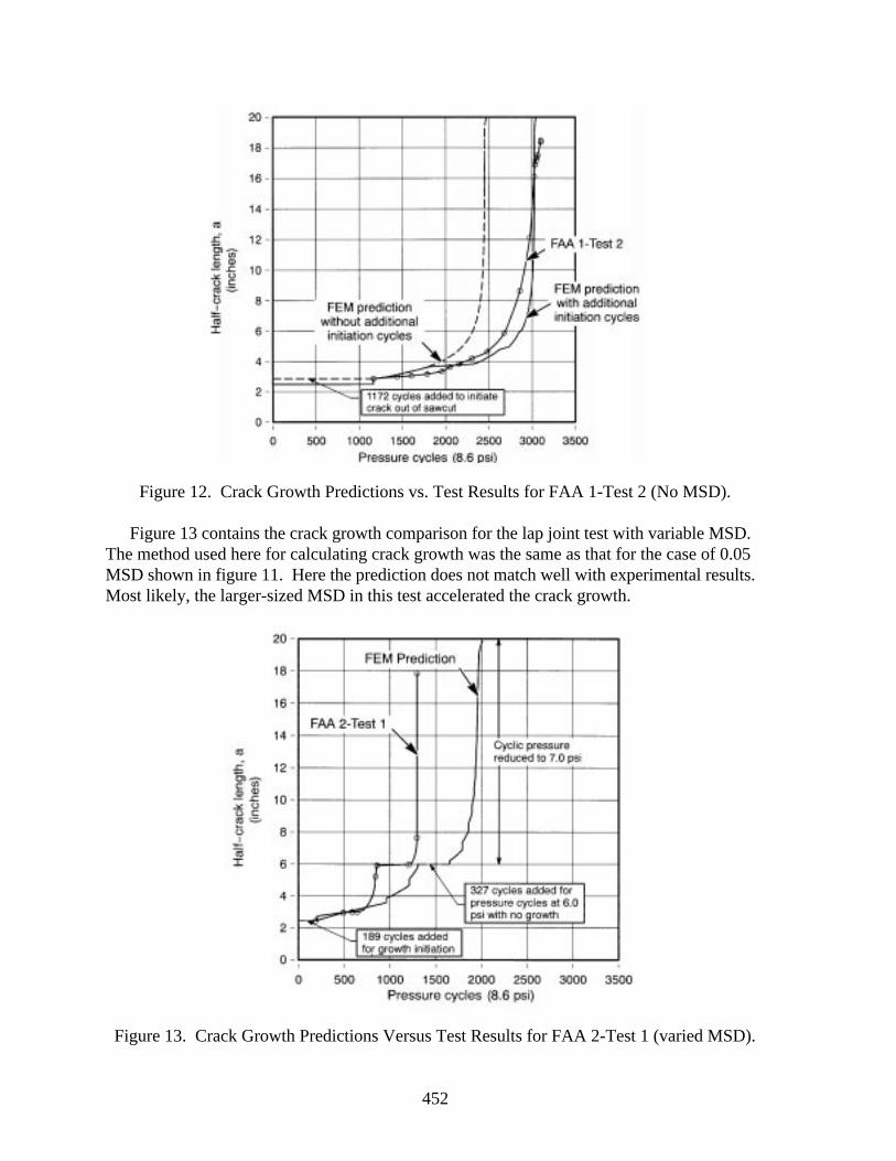
452
Figure 12. Crack Growth Predictions vs. Test Results for FAA 1-Test 2 (No MSD).
Figure 13 contains the crack growth comparison for the lap joint test with variable MSD.The method used here for calculating crack growth was the same as that for the case of 0.05MSD shown in figure 11. Here the prediction does not match well with experimental results.Most likely, the larger-sized MSD in this test accelerated the crack growth.
Figure 13. Crack Growth Predictions Versus Test Results for FAA 2-Test 1 (varied MSD).
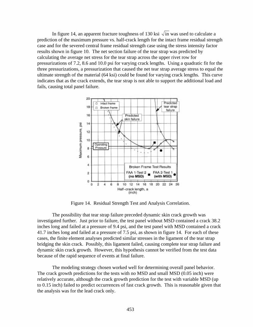
453
In figure 14, an apparent fracture toughness of 130 ksi in was used to calculate aprediction of the maximum pressure vs. half-crack length for the intact frame residual strengthcase and for the severed central frame residual strength case using the stress intensity factorresults shown in figure 10. The net section failure of the tear strap was predicted bycalculating the average net stress for the tear strap across the upper rivet row forpressurizations of 7.2, 8.6 and 10.0 psi for varying crack lengths. Using a quadratic fit for thethree pressurizations, a pressurization that caused the net tear strap average stress to equal theultimate strength of the material (64 ksi) could be found for varying crack lengths. This curveindicates that as the crack extends, the tear strap is not able to support the additional load andfails, causing total panel failure.
Figure 14. Residual Strength Test and Analysis Correlation.
The possibility that tear strap failure preceded dynamic skin crack growth wasinvestigated further. Just prior to failure, the test panel without MSD contained a crack 38.2inches long and failed at a pressure of 9.4 psi, and the test panel with MSD contained a crack41.7 inches long and failed at a pressure of 7.5 psi, as shown in figure 14. For each of thesecases, the finite element analyses predicted similar stresses in the ligament of the tear strapbridging the skin crack. Possibly, this ligament failed, causing complete tear strap failure anddynamic skin crack growth. However, this hypothesis cannot be verified from the test databecause of the rapid sequence of events at final failure.
The modeling strategy chosen worked well for determining overall panel behavior.The crack growth predictions for the tests with no MSD and small MSD (0.05 inch) wererelatively accurate, although the crack growth prediction for the test with variable MSD (upto 0.15 inch) failed to predict occurrences of fast crack growth. This is reasonable given thatthe analysis was for the lead crack only.
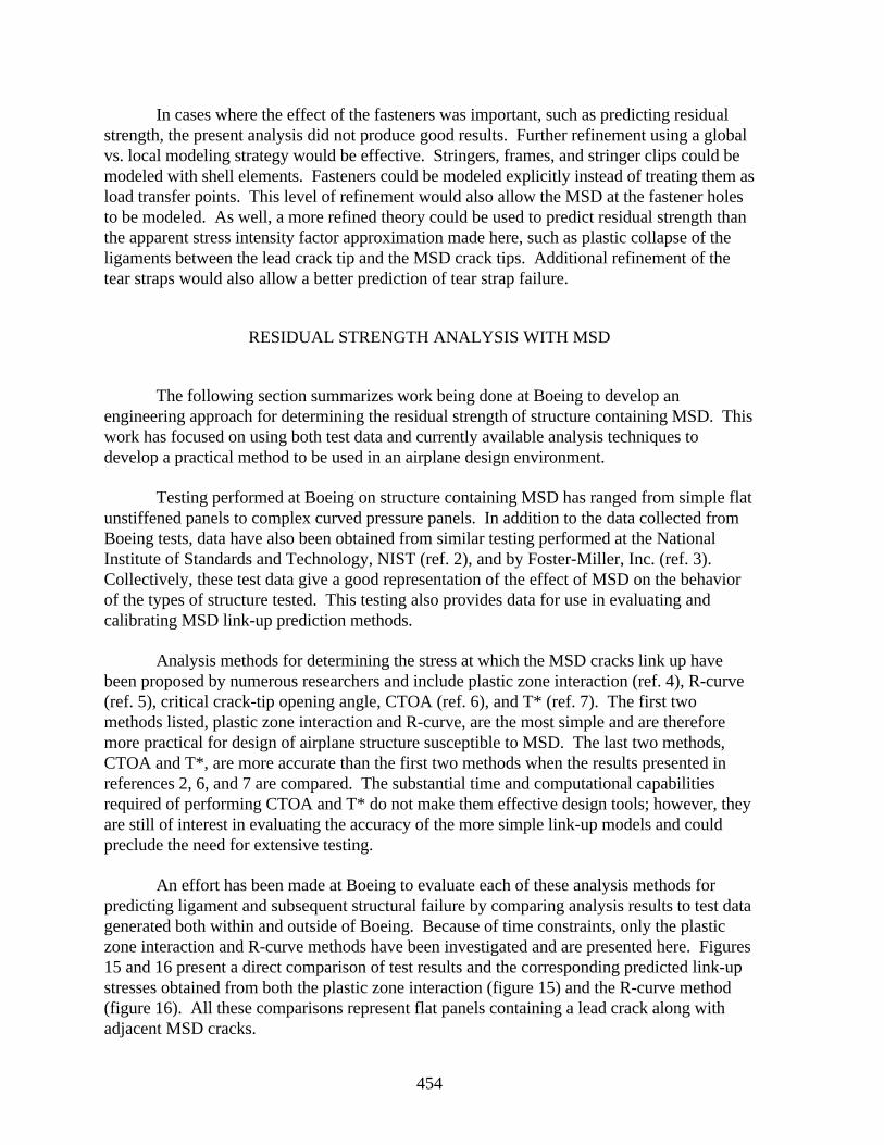
454
In cases where the effect of the fasteners was important, such as predicting residualstrength, the present analysis did not produce good results. Further refinement using a globalvs. local modeling strategy would be effective. Stringers, frames, and stringer clips could bemodeled with shell elements. Fasteners could be modeled explicitly instead of treating them asload transfer points. This level of refinement would also allow the MSD at the fastener holesto be modeled. As well, a more refined theory could be used to predict residual strength thanthe apparent stress intensity factor approximation made here, such as plastic collapse of theligaments between the lead crack tip and the MSD crack tips. Additional refinement of thetear straps would also allow a better prediction of tear strap failure.
RESIDUAL STRENGTH ANALYSIS WITH MSD
The following section summarizes work being done at Boeing to develop anengineering approach for determining the residual strength of structure containing MSD. Thiswork has focused on using both test data and currently available analysis techniques todevelop a practical method to be used in an airplane design environment.
Testing performed at Boeing on structure containing MSD has ranged from simple flatunstiffened panels to complex curved pressure panels. In addition to the data collected fromBoeing tests, data have also been obtained from similar testing performed at the NationalInstitute of Standards and Technology, NIST (ref. 2), and by Foster-Miller, Inc. (ref. 3).Collectively, these test data give a good representation of the effect of MSD on the behaviorof the types of structure tested. This testing also provides data for use in evaluating andcalibrating MSD link-up prediction methods.
Analysis methods for determining the stress at which the MSD cracks link up havebeen proposed by numerous researchers and include plastic zone interaction (ref. 4), R-curve(ref. 5), critical crack-tip opening angle, CTOA (ref. 6), and T* (ref. 7). The first twomethods listed, plastic zone interaction and R-curve, are the most simple and are thereforemore practical for design of airplane structure susceptible to MSD. The last two methods,CTOA and T*, are more accurate than the first two methods when the results presented inreferences 2, 6, and 7 are compared. The substantial time and computational capabilitiesrequired of performing CTOA and T* do not make them effective design tools; however, theyare still of interest in evaluating the accuracy of the more simple link-up models and couldpreclude the need for extensive testing.
An effort has been made at Boeing to evaluate each of these analysis methods forpredicting ligament and subsequent structural failure by comparing analysis results to test datagenerated both within and outside of Boeing. Because of time constraints, only the plasticzone interaction and R-curve methods have been investigated and are presented here. Figures15 and 16 present a direct comparison of test results and the corresponding predicted link-upstresses obtained from both the plastic zone interaction (figure 15) and the R-curve method(figure 16). All these comparisons represent flat panels containing a lead crack along withadjacent MSD cracks.
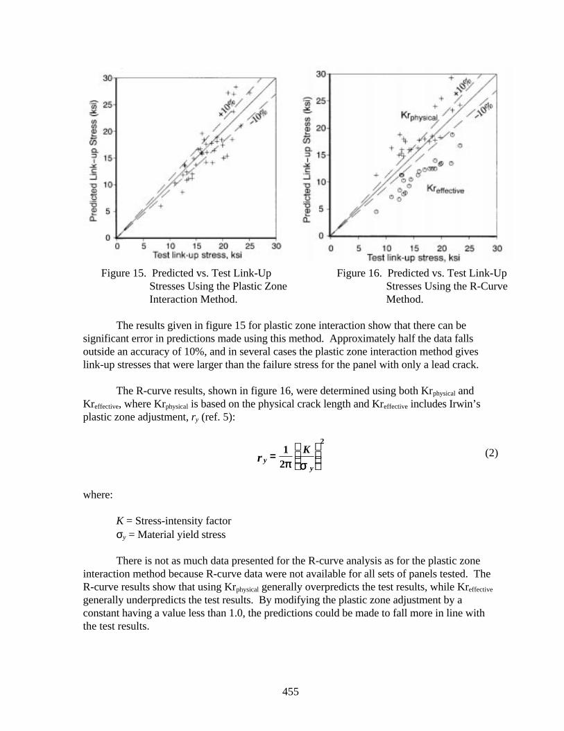
455
Figure 15. Predicted vs. Test Link-UpStresses Using the Plastic ZoneInteraction Method.
Figure 16. Predicted vs. Test Link-UpStresses Using the R-CurveMethod.
The results given in figure 15 for plastic zone interaction show that there can besignificant error in predictions made using this method. Approximately half the data fallsoutside an accuracy of 10%, and in several cases the plastic zone interaction method giveslink-up stresses that were larger than the failure stress for the panel with only a lead crack.
The R-curve results, shown in figure 16, were determined using both Krphysical andKreffective, where Krphysical is based on the physical crack length and Kreffective includes Irwin’splastic zone adjustment, ry (ref. 5):
yy
rK==
12
2
ππ σσ(2)
where:
K = Stress-intensity factorσy = Material yield stress
There is not as much data presented for the R-curve analysis as for the plastic zoneinteraction method because R-curve data were not available for all sets of panels tested. TheR-curve results show that using Krphysical generally overpredicts the test results, while Kreffective
generally underpredicts the test results. By modifying the plastic zone adjustment by aconstant having a value less than 1.0, the predictions could be made to fall more in line withthe test results.
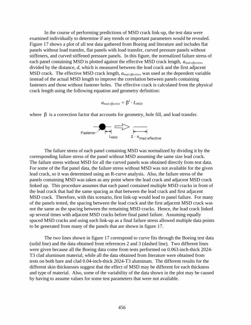
456
In the course of performing predictions of MSD crack link-up, the test data wereexamined individually to determine if any trends or important parameters would be revealed.Figure 17 shows a plot of all test data gathered from Boeing and literature and includes flatpanels without load transfer, flat panels with load transfer, curved pressure panels withoutstiffeners, and curved stiffened pressure panels. In this figure, the normalized failure stress ofeach panel containing MSD is plotted against the effective MSD crack length, amsd effective,divided by the distance, d, which is measured between the lead crack and the first adjacentMSD crack. The effective MSD crack length, amsd effective, was used as the dependent variableinstead of the actual MSD length to improve the correlation between panels containingfasteners and those without fastener holes. The effective crack is calculated from the physicalcrack length using the following equation and geometry definition:
amsd effective = β2 · LMSD
where β is a correction factor that accounts for geometry, hole fill, and load transfer.
The failure stress of each panel containing MSD was normalized by dividing it by thecorresponding failure stress of the panel without MSD assuming the same size lead crack.The failure stress without MSD for all the curved panels was obtained directly from test data.For some of the flat panel data, the failure stress without MSD was not available for the givenlead crack, so it was determined using an R-curve analysis. Also, the failure stress of thepanels containing MSD was taken as any point where the lead crack and adjacent MSD cracklinked up. This procedure assumes that each panel contained multiple MSD cracks in front ofthe lead crack that had the same spacing as that between the lead crack and first adjacentMSD crack. Therefore, with this scenario, first link-up would lead to panel failure. For manyof the panels tested, the spacing between the lead crack and the first adjacent MSD crack wasnot the same as the spacing between the remaining MSD cracks. Hence, the lead crack linkedup several times with adjacent MSD cracks before final panel failure. Assuming equallyspaced MSD cracks and using each link-up as a final failure stress allowed multiple data pointsto be generated from many of the panels that are shown in figure 17.
The two lines shown in figure 17 correspond to curve fits through the Boeing test data(solid line) and the data obtained from references 2 and 3 (dashed line). Two different lineswere given because all the Boeing data come from tests performed on 0.063-inch-thick 2024-T3 clad aluminum material, while all the data obtained from literature were obtained fromtests on both bare and clad 0.04-inch-thick 2024-T3 aluminum. The different results for thedifferent skin thicknesses suggest that the effect of MSD may be different for each thicknessand type of material. Also, some of the variability of the data shown in the plot may be causedby having to assume values for some test parameters that were not available.
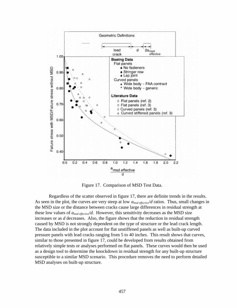
457
Figure 17. Comparison of MSD Test Data.
Regardless of the scatter observed in figure 17, there are definite trends in the results.As seen in the plot, the curves are very steep at low amsd effective/d ratios. Thus, small changes inthe MSD size or the distance between cracks cause large differences in residual strength atthese low values of amsd effective/d. However, this sensitivity decreases as the MSD sizeincreases or as d decreases. Also, the figure shows that the reduction in residual strengthcaused by MSD is not strongly dependent on the type of structure or the lead crack length.The data included in the plot account for flat unstiffened panels as well as built-up curvedpressure panels with lead cracks ranging from 5 to 40 inches. This result shows that curves,similar to those presented in figure 17, could be developed from results obtained fromrelatively simple tests or analyses performed on flat panels. These curves would then be usedas a design tool to determine the knockdown in residual strength for any built-up structuresusceptible to a similar MSD scenario. This procedure removes the need to perform detailedMSD analyses on built-up structure.
458
CONCLUSIONS
Curved Pressure Panel Testing
• The crack growth rate of the lead crack in the lap joint was greater in the presence ofsimulated MSD. Without MSD the lead crack arrested in each fastener hole, andadditional cycles were required to extend the crack out of the opposite side.
• For the floating frame panel geometry (no shear ties) and crack lengths tested in this
program, the presence of 0.05-inch MSD in the lap joint upper rivet row reduced theresidual strength of the panel by 20% compared to a panel containing no MSD.
• During the residual strength portion of the tests, the tear straps bridging the crack tips
of the two-bay lead crack remained intact until the final failure load was reached.However, the test results are inconclusive as to whether tear strap failure led todynamic extension of the lead crack.
Finite Element Analysis
• The predictions of skin and tear strap stresses and crack growth history with andwithout MSD are generally very accurate as shown in the test/analysis correlations.However, frame and stringer stresses could not be reliably predicted.
• The residual strength prediction using the R-curve and Kapp methods show that,
without MSD, the lap joint lead crack would not be expected to extend dynamically atthe pressures and crack lengths observed in the tests.
• Examination of the stresses in the tear straps bridging the crack tips of the two-bay
lead crack indicates that tear strap failure probably preceded lead crack instability forboth the MSD and non-MSD cases.
MSD Analysis
• Predicting the residual strength of structure containing MSD using simple analysismethods such as plastic zone interaction and R-curve may not provide sufficientaccuracy to be useful. However, more accurate methods such as CTOA and T* aretoo time- and resource-consuming to perform in a design environment.
• Comparing test results from various panel geometries shows that lead crack size andpanel geometry do not have a big influence on the reduction in residual strength
459/460
caused by MSD. Therefore, tests and analyses can be performed on simple panelgeometries to get an acceptable representation of the effect of MSD on the residualstrength of built-up panels.
ACKNOWLEDGMENTS
The authors would like to acknowledge the graphics and publications support fromMr. W. J. Brewer and the Boeing Support Services. We would also like to acknowledge theleadership of Mr. Chris Mazur in performing work associated with the FAA contract. Finally,we would like to thank Dr. Roland deWit for providing additional information about the 90-inch-wide flat panel tests performed at NIST.
REFERENCES
1. Gruber, M. L.; Mazur, C. J.; Wilkins, K. E.; and Worden, R. E.: Investigation ofFuselage Structure Subject to Widespread Fatigue Damage, FAA Technical Report,DOT/FAA/AR-95/47, February 1996.
2. deWit, R.; Fields, R. J.; Low III, S. R.; Harne, D. E.; and Foecke, T.: Fracture
Testing of Large-Scale Thin-Sheet Aluminum Alloy, FAA Technical Report,DOT/FAA/AR-95/11, February 1996.
3. Thomson, D.; Hoadley, D.; and McHatton, J.: Load Tests of Flat and Curved Panels
with Multiple Cracks, Foster-Miller Draft Final Report to the FAA Technical Center,September 1993.
4. Broek, D.: The Effects of Multi-Site-Damage on the Arrest Capability of Aircraft
Fuselage Structures, FractuREsearch TR9302, June 1993. 5. Broek, D.: Elementary Engineering Fracture Mechanics, Martinus Nijhoff
Publishers, Fourth Edition. 6. Newman, Jr., J. C. and Dawicke, D. S.: Fracture Analysis of Stiffened Panels Under
Biaxial Loading with Widespread Cracking, NASA TM 110197, November 1995. 7. Wang, L.; Brust, F. W.; and Atluri, S. N.: The Elastic-Plastic Finite Element
Alternating Method (EPFEAM) and the Prediction of Fracture under WFD Conditionin Aircraft Structures, Part III - Computational Predictions of the NIST Multiple SiteDamage Experimental Results, FAA Center of Excellence for ComputationalModeling of Aircraft Structures, Georgia Institute of Technology, August 1995.
461
NUMERICAL INVESTIGATIONS INTO THE VIABILITY OFCRACK TI P OPENING DISPLACEMENT AS A FRACTURE PARAMETER FOR
MIXED-MODE I/II TEARING O F THIN ALUMINUM SHEETS 1
M. A. Sutton, Wenzhong Zhao, X. DengDepartment of Mechanical Engineering
University of South CarolinaColumbia, SC
D. S. DawickeAnalytical Services and Materials, Inc.
Hampton, VA
J. C. Newman, Jr.NASA Langley Research CenterMechanics of Materials Branch
Hampton, VA
SUMMARY
Detailed two-dimensional finite element analyses of a mixed-mode I/II ARCAN testspecimen machined from 2024-T3 aluminum have been performed to assess the viability ofusing a critical crack tip opening displacement (CTOD) criterion for prediction of the load-crack extension (P-∆a) response. Preliminary results for four levels of mode mixity indicatethat (a) trends in the measured P-∆a behavior are accurately predicted throughout the crackgrowth process by the finite element analysis using experimentally determined mean CTODvalues and (b) the predicted maximum load is within 7% of the measured value for all cases.Thus, the results indicate that use of a single parameter for prediction of crack growth in thinsheet materials under complex loading conditions is feasible.
INTRODUCTION
One of the objectives of aging aircraft research is to develop models of large-scaleaeronautics structures that can accurately predict the residual strength of a damaged structure.In recent years, several researchers[1-6] have demonstrated conclusively that, under Mode Iloading, a critical value for the crack tip opening angle (CTOA) exists in the region 0.5 to 1.5mm behind the crack tip. Furthermore, use of CTOA in two-dimensional analyses
1 Support for the research through NASA NAG 1-1489
462
successfully predicts the measured P-∆a behavior for a variety of thin, ductile specimengeometries. Recently, Cordes et al.[7] used crack tip opening angle (CTOA) and the VR curveapproach in the ABAQUS numerical code to predict the fracture of compact tension (CT) andmiddle cracked tension (M(T)) specimens under Mode I loading. Their results indicated thatCTOA was more accurate in predicting the P-∆a response than the VR curve approach.
However, it is well known that cracks in aircraft fuselages undergo a combination oflocal loading conditions[8-10]. Recent modeling of aircraft fuselage structures[11] for fatiguecrack growth using a nonlinear shell code with a maximum tangential stress theory along themidplane surface to predict the direction of crack growth has shown that the fatigue cracktrajectory is reasonably predicted in the unreinforced skin region. However in the vicinity ofstructural stiffeners, where mixed-mode and deformation gradient conditions are moresevere, predictions of observed crack trajectories are more difficult.
To assess the viability of extending the concept of CTOA to mixed-mode conditions,Amstutz et al.[12-13] developed a mixed-mode I/II test specimen that is an extension of theARCAN[14] geometry used originally for composite specimens. By subjecting thin-sheet2024-T3 aluminum specimens to a wide range of mode I/II conditions while measuringCTOD in the region between 0.5 and 1.5 mm behind the crack tip, they have shown that (a) atransition from Mode I to Mode II type fracture exists, (b) CTOD is reasonably constant for∆a ≥ 10 mm for all mode mixity values and is within the range measured for LT and TLspecimens under pure mode I loading, and (c) the early stages of crack growth under mixed-mode loading show a transition towards a constant CTOD that is a function of the modemixity. Due to the scatter in the observed CTOD, as well as recent observations indicatingthat there are significant through-thickness variations in CTOD even for thin specimens[15],the viability of a critical CTOD for prediction of the P-∆a response must be viewed asundetermined.
The enclosed work presents initial results from detailed two-dimensional finiteelement analyses of the mixed-mode I/II ARCAN test specimen and fixture[12,13], which havebeen performed to assess the viability of using a critical crack tip opening displacement(CTOD) criterion for prediction of the load-crack extension (P-∆a) response.
EXPERIMENTAL RESULTS
The ARCAN test fixture and test specimen, as well as the finite element method(FEM) mesh used to model the fixture and specimen, are shown in Figure 1. The test fixturewas machined from precipitation hardened stainless steel and is nominally 12.7 mm thick.All specimens were machined from 2.4-mm-thick sheets of 2024-T3 aluminum and fatigueprecracked using controlled load shedding to minimize the initial plastic zone size[12,13];initial a/w values for all specimens were a/w = 0.167. Relevant properties for both materialsare shown in Table 1. It is noted that, due to large rotations which occurred during crack
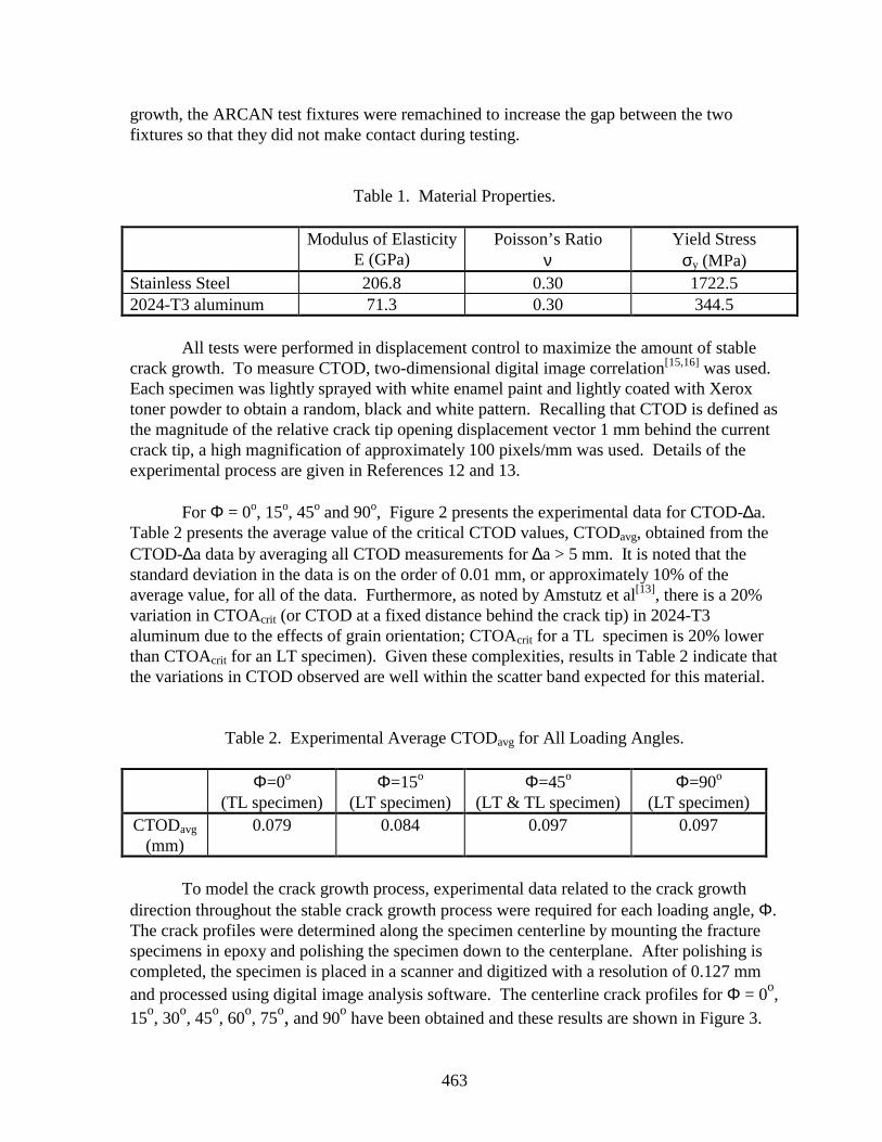
463
growth, the ARCAN test fixtures were remachined to increase the gap between the twofixtures so that they did not make contact during testing.
Table 1. Material Properties.
Modulus of ElasticityE (GPa)
Poisson’s Ratioν
Yield Stressσy (MPa)
Stainless Steel 206.8 0.30 1722.52024-T3 aluminum 71.3 0.30 344.5
All tests were performed in displacement control to maximize the amount of stablecrack growth. To measure CTOD, two-dimensional digital image correlation[15,16] was used.Each specimen was lightly sprayed with white enamel paint and lightly coated with Xeroxtoner powder to obtain a random, black and white pattern. Recalling that CTOD is defined asthe magnitude of the relative crack tip opening displacement vector 1 mm behind the currentcrack tip, a high magnification of approximately 100 pixels/mm was used. Details of theexperimental process are given in References 12 and 13.
For Φ = 0o, 15o, 45o and 90o, Figure 2 presents the experimental data for CTOD-∆a.Table 2 presents the average value of the critical CTOD values, CTODavg, obtained from theCTOD-∆a data by averaging all CTOD measurements for ∆a > 5 mm. It is noted that thestandard deviation in the data is on the order of 0.01 mm, or approximately 10% of theaverage value, for all of the data. Furthermore, as noted by Amstutz et al[13], there is a 20%variation in CTOAcrit (or CTOD at a fixed distance behind the crack tip) in 2024-T3aluminum due to the effects of grain orientation; CTOAcrit for a TL specimen is 20% lowerthan CTOAcrit for an LT specimen). Given these complexities, results in Table 2 indicate thatthe variations in CTOD observed are well within the scatter band expected for this material.
Table 2. Experimental Average CTODavg for All Loading Angles.
Φ=0o
(TL specimen)Φ=15o
(LT specimen)Φ=45o
(LT & TL specimen)Φ=90o
(LT specimen)CTODavg
(mm)0.079 0.084 0.097 0.097
To model the crack growth process, experimental data related to the crack growthdirection throughout the stable crack growth process were required for each loading angle, Φ.The crack profiles were determined along the specimen centerline by mounting the fracturespecimens in epoxy and polishing the specimen down to the centerplane. After polishing iscompleted, the specimen is placed in a scanner and digitized with a resolution of 0.127 mmand processed using digital image analysis software. The centerline crack profiles for Φ = 0o,15o, 30o, 45o, 60o, 75o, and 90o have been obtained and these results are shown in Figure 3.
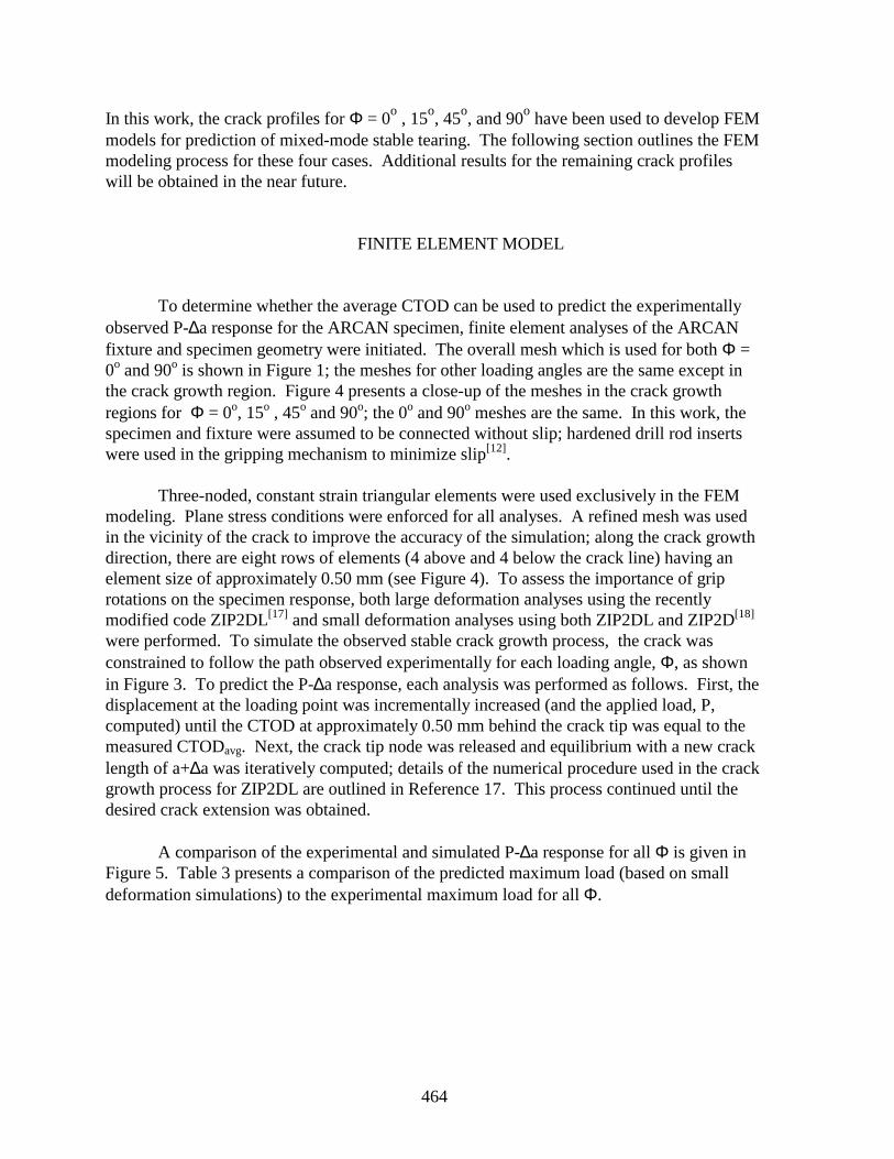
464
In this work, the crack profiles for Φ = 0o , 15o, 45o, and 90o have been used to develop FEMmodels for prediction of mixed-mode stable tearing. The following section outlines the FEMmodeling process for these four cases. Additional results for the remaining crack profileswill be obtained in the near future.
FINITE ELEMENT MODEL
To determine whether the average CTOD can be used to predict the experimentallyobserved P-∆a response for the ARCAN specimen, finite element analyses of the ARCANfixture and specimen geometry were initiated. The overall mesh which is used for both Φ =0o and 90o is shown in Figure 1; the meshes for other loading angles are the same except inthe crack growth region. Figure 4 presents a close-up of the meshes in the crack growthregions for Φ = 0o, 15o , 45o and 90o; the 0o and 90o meshes are the same. In this work, thespecimen and fixture were assumed to be connected without slip; hardened drill rod insertswere used in the gripping mechanism to minimize slip[12].
Three-noded, constant strain triangular elements were used exclusively in the FEMmodeling. Plane stress conditions were enforced for all analyses. A refined mesh was usedin the vicinity of the crack to improve the accuracy of the simulation; along the crack growthdirection, there are eight rows of elements (4 above and 4 below the crack line) having anelement size of approximately 0.50 mm (see Figure 4). To assess the importance of griprotations on the specimen response, both large deformation analyses using the recentlymodified code ZIP2DL[17] and small deformation analyses using both ZIP2DL and ZIP2D[18]
were performed. To simulate the observed stable crack growth process, the crack wasconstrained to follow the path observed experimentally for each loading angle, Φ, as shownin Figure 3. To predict the P-∆a response, each analysis was performed as follows. First, thedisplacement at the loading point was incrementally increased (and the applied load, P,computed) until the CTOD at approximately 0.50 mm behind the crack tip was equal to themeasured CTODavg. Next, the crack tip node was released and equilibrium with a new cracklength of a+∆a was iteratively computed; details of the numerical procedure used in the crackgrowth process for ZIP2DL are outlined in Reference 17. This process continued until thedesired crack extension was obtained.
A comparison of the experimental and simulated P-∆a response for all Φ is given inFigure 5. Table 3 presents a comparison of the predicted maximum load (based on smalldeformation simulations) to the experimental maximum load for all Φ.
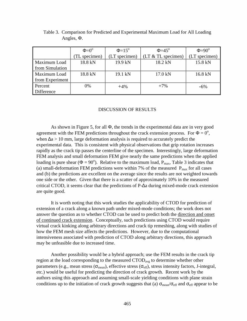
465
Table 3. Comparison for Predicted and Experimental Maximum Load for All LoadingAngles, Φ.
Φ=0o
(TL specimen)Φ=15o
(LT specimen)Φ=45o
(LT & TL specimen)Φ=90o
(LT specimen)Maximum Loadfrom Simulation
18.8 kN 19.9 kN 18.2 kN 15.8 kN
Maximum Loadfrom Experiment
18.8 kN 19.1 kN 17.0 kN 16.8 kN
PercentDifference
0% +4% +7% -6%
DISCUSSION OF RESULTS
As shown in Figure 5, for all Φ, the trends in the experimental data are in very goodagreement with the FEM predictions throughout the crack extension process. For Φ = 0o,when ∆a > 10 mm, large deformation analysis is required to accurately predict theexperimental data. This is consistent with physical observations that grip rotation increasesrapidly as the crack tip passes the centerline of the specimen. Interestingly, large deformationFEM analysis and small deformation FEM give nearly the same predictions when the appliedloading is pure shear (Φ = 90o). Relative to the maximum load, Pmax, Table 3 indicates that(a) small-deformation FEM predictions were within 7% of the measured Pmax for all casesand (b) the predictions are excellent on the average since the results are not weighted towardsone side or the other. Given that there is a scatter of approximately 10% in the measuredcritical CTOD, it seems clear that the predictions of P-∆a during mixed-mode crack extensionare quite good.
It is worth noting that this work studies the applicability of CTOD for prediction ofextension of a crack along a known path under mixed-mode conditions; the work does notanswer the question as to whether CTOD can be used to predict both the direction and onsetof continued crack extension. Conceptually, such predictions using CTOD would requirevirtual crack kinking along arbitrary directions and crack tip remeshing, along with studies ofhow the FEM mesh size affects the predictions. However, due to the computationalintensiveness associated with prediction of CTOD along arbitrary directions, this approachmay be unfeasible due to increased time.
Another possibility would be a hybrid approach; use the FEM results in the crack tipregion at the load corresponding to the measured CTODavg to determine whether otherparameters (e.g., mean stress (σmean), effective stress (σeff), stress intensity factors, J-integral,etc.) would be useful for predicting the direction of crack growth. Recent work by theauthors using this approach and assuming small-scale yielding conditions with plane strainconditions up to the initiation of crack growth suggests that (a) σmean/σeff and σeff appear to be
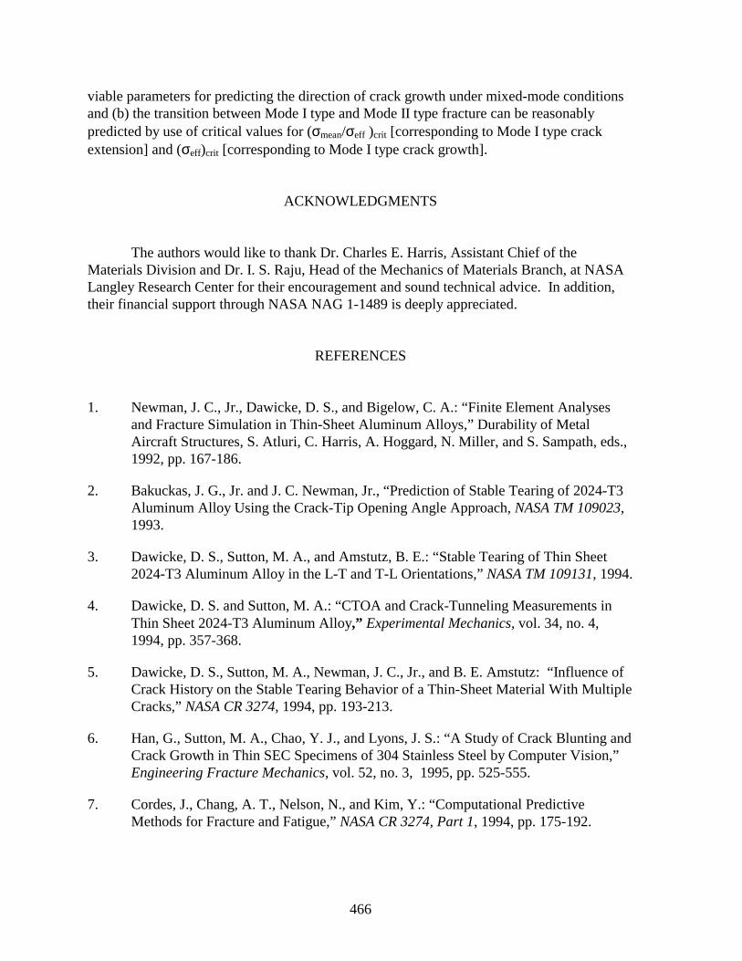
466
viable parameters for predicting the direction of crack growth under mixed-mode conditionsand (b) the transition between Mode I type and Mode II type fracture can be reasonablypredicted by use of critical values for (σmean/σeff )crit [corresponding to Mode I type crackextension] and (σeff)crit [corresponding to Mode I type crack growth].
ACKNOWLEDGMENTS
The authors would like to thank Dr. Charles E. Harris, Assistant Chief of theMaterials Division and Dr. I. S. Raju, Head of the Mechanics of Materials Branch, at NASALangley Research Center for their encouragement and sound technical advice. In addition,their financial support through NASA NAG 1-1489 is deeply appreciated.
REFERENCES
1. Newman, J. C., Jr., Dawicke, D. S., and Bigelow, C. A.: “Finite Element Analysesand Fracture Simulation in Thin-Sheet Aluminum Alloys,” Durability of MetalAircraft Structures, S. Atluri, C. Harris, A. Hoggard, N. Miller, and S. Sampath, eds.,1992, pp. 167-186.
2. Bakuckas, J. G., Jr. and J. C. Newman, Jr., “Prediction of Stable Tearing of 2024-T3Aluminum Alloy Using the Crack-Tip Opening Angle Approach, NASA TM 109023,1993.
3. Dawicke, D. S., Sutton, M. A., and Amstutz, B. E.: “Stable Tearing of Thin Sheet2024-T3 Aluminum Alloy in the L-T and T-L Orientations,” NASA TM 109131, 1994.
4. Dawicke, D. S. and Sutton, M. A.: “CTOA and Crack-Tunneling Measurements inThin Sheet 2024-T3 Aluminum Alloy,” Experimental Mechanics, vol. 34, no. 4,1994, pp. 357-368.
5. Dawicke, D. S., Sutton, M. A., Newman, J. C., Jr., and B. E. Amstutz: “Influence ofCrack History on the Stable Tearing Behavior of a Thin-Sheet Material With MultipleCracks,” NASA CR 3274, 1994, pp. 193-213.
6. Han, G., Sutton, M. A., Chao, Y. J., and Lyons, J. S.: “A Study of Crack Blunting andCrack Growth in Thin SEC Specimens of 304 Stainless Steel by Computer Vision,”Engineering Fracture Mechanics, vol. 52, no. 3, 1995, pp. 525-555.
7. Cordes, J., Chang, A. T., Nelson, N., and Kim, Y.: “Computational PredictiveMethods for Fracture and Fatigue,” NASA CR 3274, Part 1, 1994, pp. 175-192.
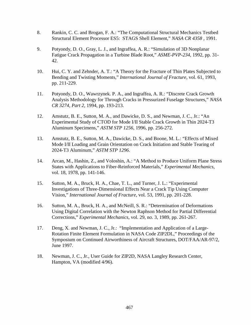
467
8. Rankin, C. C. and Brogan, F. A.: “The Computational Structural Mechanics TestbedStructural Element Processor ES5: STAGS Shell Element,” NASA CR 4358 , 1991.
9. Potyondy, D. O., Gray, L. J., and Ingraffea, A. R.: “Simulation of 3D NonplanarFatigue Crack Propagation in a Turbine Blade Root,” ASME-PVP-234, 1992, pp. 31-42.
10. Hui, C. Y. and Zehnder, A. T.: “A Theory for the Fracture of Thin Plates Subjected toBending and Twisting Moments,” International Journal of Fracture, vol. 61, 1993,pp. 211-229.
11. Potyondy, D. O., Wawrzynek. P. A., and Ingraffea, A. R.: “Discrete Crack GrowthAnalysis Methodology for Through Cracks in Pressurized Fuselage Structures,” NASACR 3274, Part 2, 1994, pp. 193-213.
12. Amstutz, B. E., Sutton, M. A., and Dawicke, D. S., and Newman, J. C., Jr.: “AnExperimental Study of CTOD for Mode I/II Stable Crack Growth in Thin 2024-T3Aluminum Specimens,” ASTM STP 1256, 1996, pp. 256-272.
13. Amstutz, B. E., Sutton, M. A., Dawicke, D. S., and Boone, M. L.: “Effects of MixedMode I/II Loading and Grain Orientation on Crack Initiation and Stable Tearing of2024-T3 Aluminum,” ASTM STP 1296.
14. Arcan, M., Hashin, Z., and Voloshin, A.: “A Method to Produce Uniform Plane StressStates with Applications to Fiber-Reinforced Materials,” Experimental Mechanics,vol. 18, 1978, pp. 141-146.
15. Sutton, M. A., Bruck, H. A., Chae, T. L., and Turner, J. L.: “ExperimentalInvestigations of Three-Dimensional Effects Near a Crack Tip Using ComputerVision,” International Journal of Fracture, vol. 53, 1991, pp. 201-228.
16. Sutton, M. A., Bruck, H. A., and McNeill, S. R.: “Determination of DeformationsUsing Digital Correlation with the Newton Raphson Method for Partial DifferentialCorrections,” Experimental Mechanics, vol. 29, no. 3, 1989, pp. 261-267.
17. Deng, X. and Newman, J. C., Jr.: “Implementation and Application of a Large-Rotation Finite Element Formulation in NASA Code ZIP2DL,” Proceedings of theSymposium on Continued Airworthiness of Aircraft Structures, DOT/FAA/AR-97/2,June 1997.
18. Newman, J. C., Jr., User Guide for ZIP2D, NASA Langley Research Center,Hampton, VA (modified 4/96).
468
Figure 1. ARCAN Fixture and Specimen with FEM Mesh.
469
z
z
z
z
zz
zz
z
z
z
z
z
zz
zz
0
0.05
0.1
0.15
0.2
0.25
0 5 10 15 20 25
z
z
z
z
z
zzzz
z
z
z
zz
z
z
z
0
0.05
0.1
0.15
0.2
0.25
0 5 10 15 20 25
z LT
TL
z
z
z
z
z
z
z
z
z
zz
z
z
zz
z
zz
z
z
z
0
0.05
0.1
0.15
0.2
0.25
0 5 10 15 20 25
zz
z
z
z
z
zz
z
z
z
z
z z
zz z
zz z
0
0.05
0.1
0.15
0.2
0.25
0 5 10 15 20 25∆a (mm) ∆a (mm)
∆a (mm) ∆a (mm)
Figure 2CTOD as a Function of Crack Extension for Various
Loading Angles Φ
Φ=45° Φ=90°, LT Specimen
Φ=0°, TL Specimen Φ=15°, LT Specimen
Figure 2. CTOD as a Function of Crack Extension for Various Loading Angles, Φ.
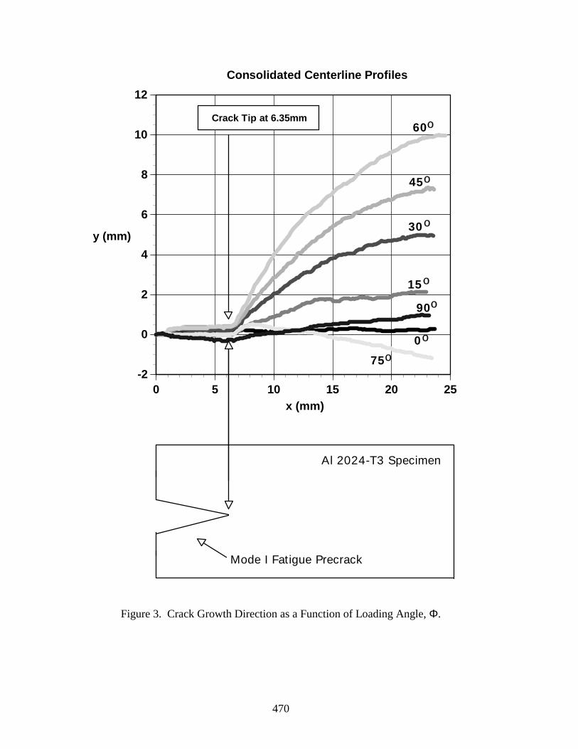
470
-2
0
2
4
6
8
10
12
0 5 10 15 20 25
y (mm)
x (mm)
Crack Tip at 6.35mm
Consolidated Centerline Profiles
Mode I Fatigue Precrack
Al 2024-T 3 S pecimen
45
75
0
15
30
60
ο
ο
ο
ο
ο
ο
90ο
Figure 3. Crack Growth Direction as a Function of Loading Angle, Φ.
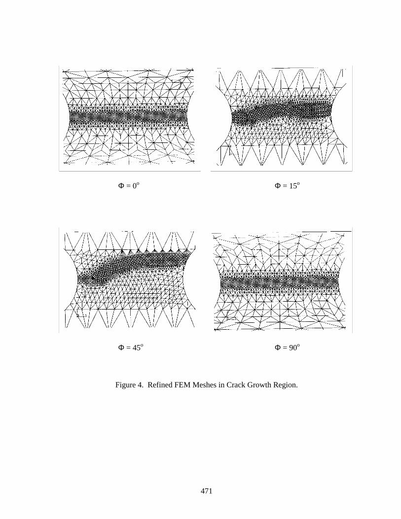
471
Φ = 0o Φ = 15o
Φ = 45o Φ = 90o
Figure 4. Refined FEM Meshes in Crack Growth Region.
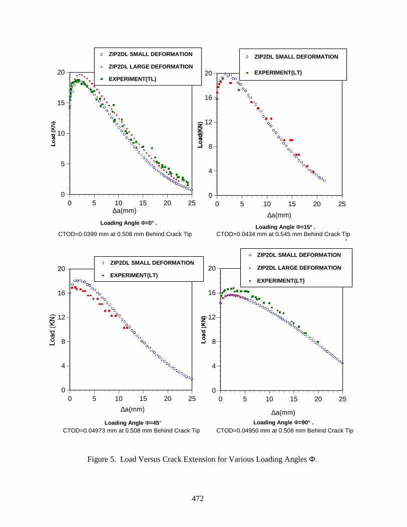
472
0
4
8
12
16
20
0 5 10 15 20 25
ZIP2DL SMALL DEFORMATION
EXPERIMENT(LT)
Figure 5Load versus Crack Extension for Various Loading Angles Φ
∆a(mm)
0
5
10
15
20
0 5 10 15 20 25
ZIP2DL SMALL DEFORMATION
ZIP2DL LARGE DEFORMATION
EXPERIMENT(TL)
∆a(mm)
0
4
8
12
16
20
0 5 10 15 20 25
ZIP2DL SMALL DEFORMATION
ZIP2DL LARGE DEFORMATION
EXPERIMENT(LT)
Loading Angle Φ=0° .
CTOD=0.0399mm at 0.508mm Behind Crack TipLoading Angle Φ=15° .
CTOD=0.0434mm at 0.545mm Behind Crack Tip
∆a(mm)Loading Angle Φ=90° .
CTOD=0.04950mm at 0.508mm Behind Crack Tip
0
4
8
12
16
20
0 5 10 15 20 25
ZIP2DL SMALL DEFORMATION
EXPERIMENT(LT)
∆a(mm)
Loading Angle Φ=45°
CTOD=0.04973 mm at 0.508mm Behind Crack Tip
CTOD=0.0434 mm at 0.545 mm Behind Crack TipCTOD=0.0399 mm at 0.508 mm Behind Crack Tip
CTOD=0.04950 mm at 0.508 mm Behind Crack Tip
Figure 5. Load Versus Crack Extension for Various Loading Angles Φ.
CTOD=0.04973 mm at 0.508 mm Behind Crack Tip
473
A NUMERICAL STUDY OF THE INTERACTIONS BETWEENMULTIPLE LONGITUDINAL CRACKS IN A FUSELAGE
(MULTIPLE DISCRETE-SOURCE DAMAGES)
W. T. Chow, L. Wang, H. Kawai, and S. N. AtluriFAA Center of Excellence for
Computational Modeling of Aircraft StructuresGeorgia Institute of Technology, Atlanta, GA
SUMMARY
The purpose of this paper is to analyze the residual strength of a pressurized fuselagepanel with multiple cracks in the longitudinal direction. Numerical studies based on theglobal-intermediate-local hierarchical process to model a full-scale fuselage panel have beencarried out to understand the interactions of multiple cracks in a stiffened structure. Thesestudies demonstrate the importance of performing an elastic-plastic analysis to obtain aconservative estimate of the residual strength of a fuselage panel. For the example of a two-bay longitudinal crack, the calculated residual strength based on the linear elastic assumption,on an average, is 30% higher than the solution based on the elastic-plastic assumption, andhence the linear elastic solution is anticonservative. In addition, the two-bay crack has beenplaced at three different locations to examine the effect that the crack location would have onthe overall residual strength. It has been found that the residual strength of a two-bay crackexisting on top of a stringer is significantly lower than the residual strength of a two-bay crackin a lap joint and that for a two-bay crack between two stringers. A study has been performedto examine the interaction between a two-bay crack and a single-bay crack separated by aframe section. The study found that the interaction between these two cracks is quite smalluntil the crack tips of the two interacting cracks are about 2 inches apart. In addition, studieshave also been carried out to understand the effect of multiple smaller cracks in front of atwo-bay lead crack. The elastic-plastic analyses have shown that cracks with the size of only1 inch can reduce the residual strength of the lead crack by half when these cracks are one-halfinch apart. Furthermore, it has been found that when the same analyses are performed usingthe linear elastic assumption, the residual strength would be underestimated by a factor oftwo. Similar studies are also carried out to examine the effect of the interactions of multiple-site damage (MSD) cracks with the two-bay crack.
INTRODUCTION
For the past two decades, the damage tolerance requirement of a fuselage section hasbeen set as the ability of the stiffened structure to contain a two-bay crack either in thelongitudinal or circumferential direction from unstable crack propagation, as shown in
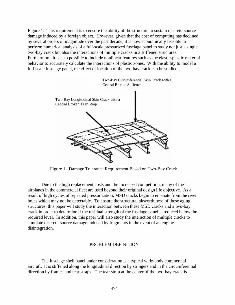
474
Figure 1. This requirement is to ensure the ability of the structure to sustain discrete-sourcedamage induced by a foreign object. However, given that the cost of computing has declinedby several orders of magnitude over the past decade, it is now economically feasible toperform numerical analysis of a full-scale pressurized fuselage panel to study not just a singletwo-bay crack but also the interactions of multiple cracks in a stiffened structures.Furthermore, it is also possible to include nonlinear features such as the elastic-plastic materialbehavior to accurately calculate the interactions of plastic zones. With the ability to model afull-scale fuselage panel, the effect of location of the two-bay crack can be studied.
Figure 1. Damage Tolerance Requirement Based on Two-Bay Crack.
Due to the high replacement costs and the increased competition, many of theairplanes in the commercial fleet are used beyond their original design life objective. As aresult of high cycles of repeated pressurization, MSD cracks begin to emanate from the rivetholes which may not be detectable. To ensure the structural airworthiness of these agingstructures, this paper will study the interaction between these MSD cracks and a two-baycrack in order to determine if the residual strength of the fuselage panel is reduced below therequired level. In addition, this paper will also study the interaction of multiple cracks tosimulate discrete-source damage induced by fragments in the event of an enginedisintegration.
PROBLEM DEFINITION
The fuselage shell panel under consideration is a typical wide-body commercialaircraft. It is stiffened along the longitudinal direction by stringers and in the circumferentialdirection by frames and tear straps. The tear strap at the center of the two-bay crack is
Two-Bay Circumferential Skin Crack with aCentral Broken Stiffener
Two-Bay Longitudinal Skin Crack with aCentral Broken Tear Strap
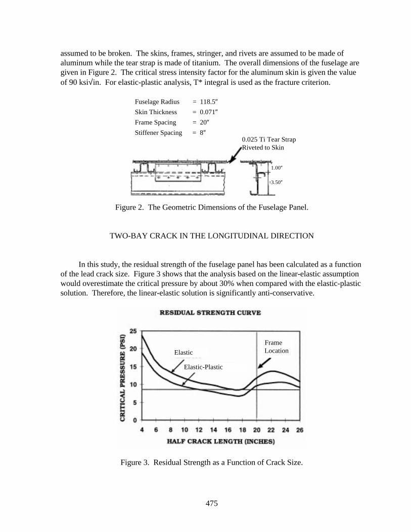
475
assumed to be broken. The skins, frames, stringer, and rivets are assumed to be made ofaluminum while the tear strap is made of titanium. The overall dimensions of the fuselage aregiven in Figure 2. The critical stress intensity factor for the aluminum skin is given the valueof 90 ksi√in. For elastic-plastic analysis, T* integral is used as the fracture criterion.
Figure 2. The Geometric Dimensions of the Fuselage Panel.
TWO-BAY CRACK IN THE LONGITUDINAL DIRECTION
In this study, the residual strength of the fuselage panel has been calculated as a functionof the lead crack size. Figure 3 shows that the analysis based on the linear-elastic assumptionwould overestimate the critical pressure by about 30% when compared with the elastic-plasticsolution. Therefore, the linear-elastic solution is significantly anti-conservative.
Figure 3. Residual Strength as a Function of Crack Size.
Fuselage Radius = 118.5″Skin Thickness = 0.071″Frame Spacing = 20″Stiffener Spacing = 8″
1.00″
3.50″
Elastic
Elastic-Plastic
Frame Location
0.025 Ti Tear StrapRiveted to Skin
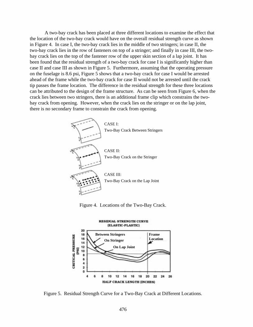
476
A two-bay crack has been placed at three different locations to examine the effect thatthe location of the two-bay crack would have on the overall residual strength curve as shownin Figure 4. In case I, the two-bay crack lies in the middle of two stringers; in case II, thetwo-bay crack lies in the row of fasteners on top of a stringer; and finally in case III, the two-bay crack lies on the top of the fastener row of the upper skin section of a lap joint. It hasbeen found that the residual strength of a two-bay crack for case I is significantly higher thancase II and case III as shown in Figure 5. Furthermore, assuming that the operating pressureon the fuselage is 8.6 psi, Figure 5 shows that a two-bay crack for case I would be arrestedahead of the frame while the two-bay crack for case II would not be arrested until the cracktip passes the frame location. The difference in the residual strength for these three locationscan be attributed to the design of the frame structure. As can be seen from Figure 6, when thecrack lies between two stringers, there is an additional frame clip which constrains the two-bay crack from opening. However, when the crack lies on the stringer or on the lap joint,there is no secondary frame to constrain the crack from opening.
Figure 4. Locations of the Two-Bay Crack.
Figure 5. Residual Strength Curve for a Two-Bay Crack at Different Locations.
CASE I:
Two-Bay Crack Between Stringers
CASE II:
Two-Bay Crack on the Stringer
CASE III:
Two-Bay Crack on the Lap Joint
Between Stringers
On Stringer
On Lap Joint
FrameLocation

477
Figure 6. The Effect of Frame Design in the Residual Strength of a Two-Bay Crack.
INTERACTION OF MULTIPLE CRACKS
The first study concerns the interaction of a two-bay crack with a single-bay crack.Both of these cracks lie in the middle between two stringers. The center of the two-bay crackwould lie on the frame while the center of the single-bay crack would lie in the middle of thebay. The sizes of these two cracks are varied such that both crack tips have an equal distance,d, to the frame position as shown in Figure 7. The result from Figure 7 shows littleinteraction between these two cracks when the distance between the two crack tips is morethan 4 in. apart even though the size of the lead crack may be as large as 36 in. However,when these two crack tips are only 2 inches apart, the residual strength of the fuselage panel isreduced by more than 20%. The strong interaction between these two cracks can beattributed to the fact that the plastic zones for these two crack tips are interacting with eachother.
Case II: Crack on Stringer Case III: Crack on Lap Joint
Case I: Crack Between Stringers
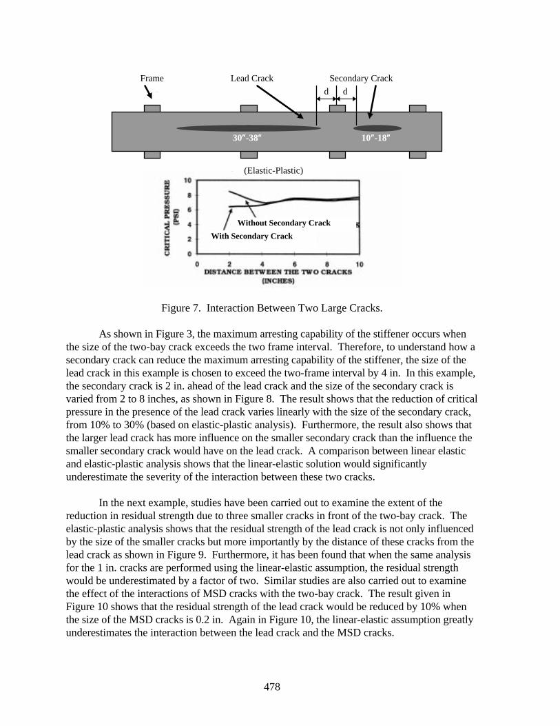
478
Figure 7. Interaction Between Two Large Cracks.
As shown in Figure 3, the maximum arresting capability of the stiffener occurs whenthe size of the two-bay crack exceeds the two frame interval. Therefore, to understand how asecondary crack can reduce the maximum arresting capability of the stiffener, the size of thelead crack in this example is chosen to exceed the two-frame interval by 4 in. In this example,the secondary crack is 2 in. ahead of the lead crack and the size of the secondary crack isvaried from 2 to 8 inches, as shown in Figure 8. The result shows that the reduction of criticalpressure in the presence of the lead crack varies linearly with the size of the secondary crack,from 10% to 30% (based on elastic-plastic analysis). Furthermore, the result also shows thatthe larger lead crack has more influence on the smaller secondary crack than the influence thesmaller secondary crack would have on the lead crack. A comparison between linear elasticand elastic-plastic analysis shows that the linear-elastic solution would significantlyunderestimate the severity of the interaction between these two cracks.
In the next example, studies have been carried out to examine the extent of thereduction in residual strength due to three smaller cracks in front of the two-bay crack. Theelastic-plastic analysis shows that the residual strength of the lead crack is not only influencedby the size of the smaller cracks but more importantly by the distance of these cracks from thelead crack as shown in Figure 9. Furthermore, it has been found that when the same analysisfor the 1 in. cracks are performed using the linear-elastic assumption, the residual strengthwould be underestimated by a factor of two. Similar studies are also carried out to examinethe effect of the interactions of MSD cracks with the two-bay crack. The result given inFigure 10 shows that the residual strength of the lead crack would be reduced by 10% whenthe size of the MSD cracks is 0.2 in. Again in Figure 10, the linear-elastic assumption greatlyunderestimates the interaction between the lead crack and the MSD cracks.
30″″-38″″ 10″″-18″″
Frame Lead Crack Secondary Crack
Without Secondary Crack
With Secondary Crack
(Elastic-Plastic)
d d
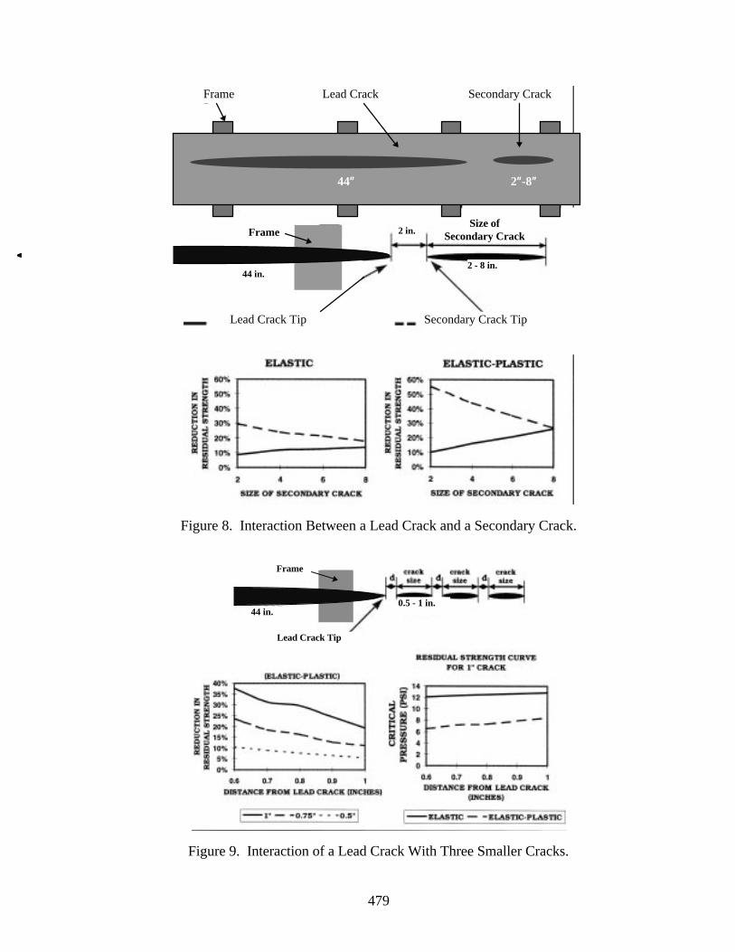
479
Figure 8. Interaction Between a Lead Crack and a Secondary Crack.
Figure 9. Interaction of a Lead Crack With Three Smaller Cracks.
2 - 8 in.
2 in.
44 in.0.5 - 1 in.
Frame Lead Crack Secondary Crack
Size ofSecondary Crack
44″″ 2″″-8″″
Lead Crack Tip Secondary Crack Tip
Frame
Lead Crack Tip
44 in.
Frame
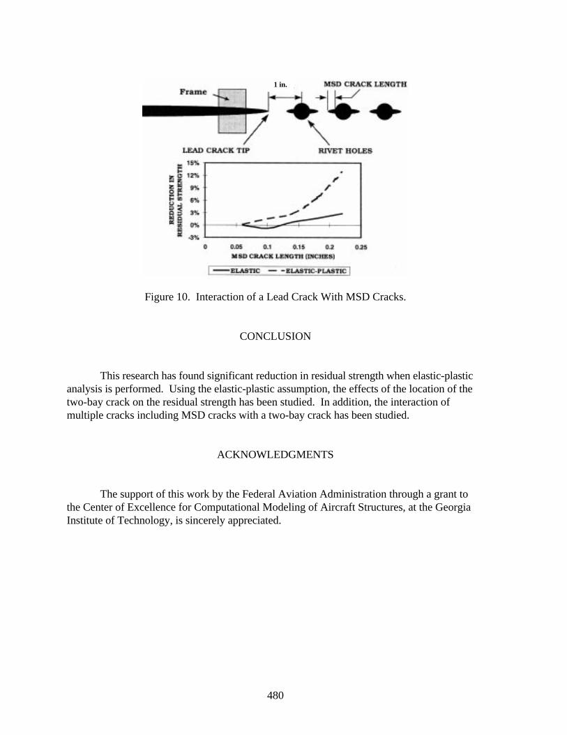
480
Frame
Lead Crack Tip
Figure 10. Interaction of a Lead Crack With MSD Cracks.
CONCLUSION
This research has found significant reduction in residual strength when elastic-plasticanalysis is performed. Using the elastic-plastic assumption, the effects of the location of thetwo-bay crack on the residual strength has been studied. In addition, the interaction ofmultiple cracks including MSD cracks with a two-bay crack has been studied.
ACKNOWLEDGMENTS
The support of this work by the Federal Aviation Administration through a grant tothe Center of Excellence for Computational Modeling of Aircraft Structures, at the GeorgiaInstitute of Technology, is sincerely appreciated.
1 in.
481
ON-AIRCRA FT ANALYSIS O F F-14 AIRCRAFT WING BEARINGSUSING ACOUSTIC EMISSION TECHNIQUES *
Donald J. Pointer, W. Drew Martin, and Adriano F. AlmeidaPhysical Acoustics Corporation
P.O. Box 3135Princeton, NJ 08543
SUMMARY
Wing pivot bearings on several F-14 aircraft were tested in situ using acoustic emission(AE) before and after rework at the Naval Aviation Depot in Norfolk, VA. Acoustic emissiondata (mainly due to friction and binding) was recorded during the wing sweep operation whilethe aircraft were undergoing depot maintenance. The six-month project demonstrated that it isfeasible to use AE for detecting friction signals and locating binding within the wing pivotbearings. The acoustic emission method was not only able to find which bearings were binding,but could also locate where the binding was taking place (on the bearing itself).
INTRODUCTION
The wing pivot bearings and the wing box found in variable swept wing designs arevital aircraft components since they must transfer complicated wing forces and moments to thefuselage. These intricate components are difficult to access and presently require thedisassembly of the wing in order to service or replace. The limited access to the F-14 wingpivot joint hinders the safety-of-flight maintenance schedule and increases costs as well asmaintenance time and total aircraft down time. The Navy’s F-14 wing pivot bearings arecurrently being changed according to a time schedule or when wing sweeping causes excessivenoise in the bearing. There are two problems with this method. First, the replacement of thebearing on a periodic schedule is costly, since not all bearings are faulty. Second, some wingpivot bearings fail before the scheduled replacement time. These faulty bearings on operatingaircraft could bind, thus causing structural problems to the surrounding wing or box beam. If afailure of this type should occur, both the pilot and aircraft would be at risk.
The goal of the Phase I contract was to prove the feasibility of using acoustic emissiontechniques to determine bearing condition and locate problem bearings. The long term goalsare stated below:
• To develop a nonintrusive, in situ method of inspection
* DoD Navy SBIR Phase I Contract Number N00189-94-C-0099
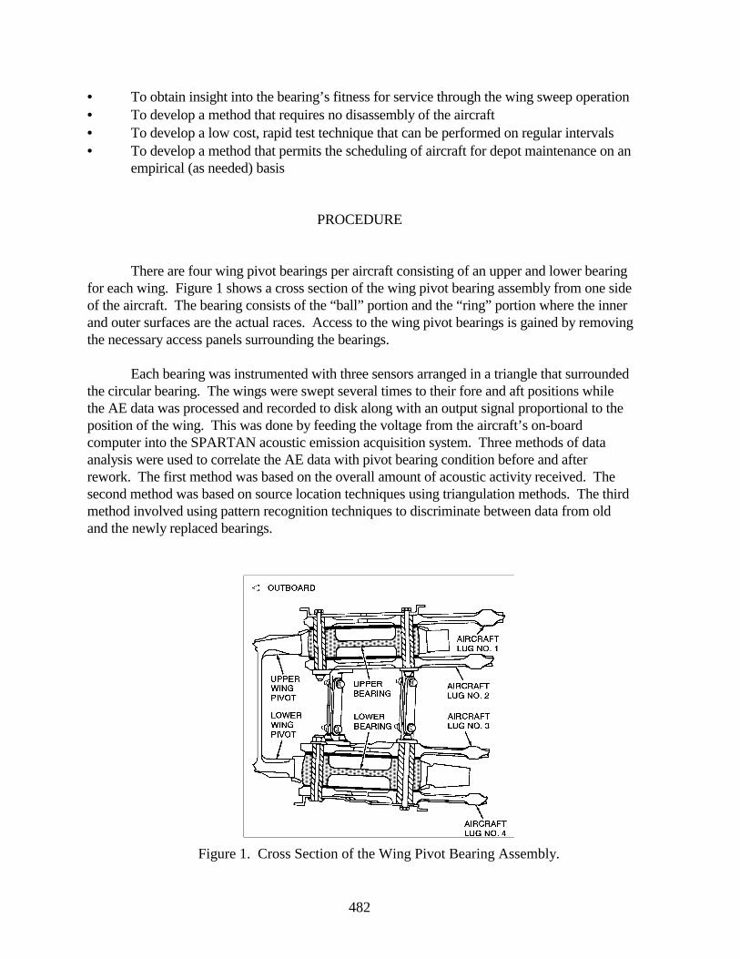
482
• To obtain insight into the bearing’s fitness for service through the wing sweep operation• To develop a method that requires no disassembly of the aircraft• To develop a low cost, rapid test technique that can be performed on regular intervals• To develop a method that permits the scheduling of aircraft for depot maintenance on an
empirical (as needed) basis
PROCEDURE
There are four wing pivot bearings per aircraft consisting of an upper and lower bearingfor each wing. Figure 1 shows a cross section of the wing pivot bearing assembly from one sideof the aircraft. The bearing consists of the “ball” portion and the “ring” portion where the innerand outer surfaces are the actual races. Access to the wing pivot bearings is gained by removingthe necessary access panels surrounding the bearings.
Each bearing was instrumented with three sensors arranged in a triangle that surroundedthe circular bearing. The wings were swept several times to their fore and aft positions whilethe AE data was processed and recorded to disk along with an output signal proportional to theposition of the wing. This was done by feeding the voltage from the aircraft’s on-boardcomputer into the SPARTAN acoustic emission acquisition system. Three methods of dataanalysis were used to correlate the AE data with pivot bearing condition before and afterrework. The first method was based on the overall amount of acoustic activity received. Thesecond method was based on source location techniques using triangulation methods. The thirdmethod involved using pattern recognition techniques to discriminate between data from oldand the newly replaced bearings.
Figure 1. Cross Section of the Wing Pivot Bearing Assembly.
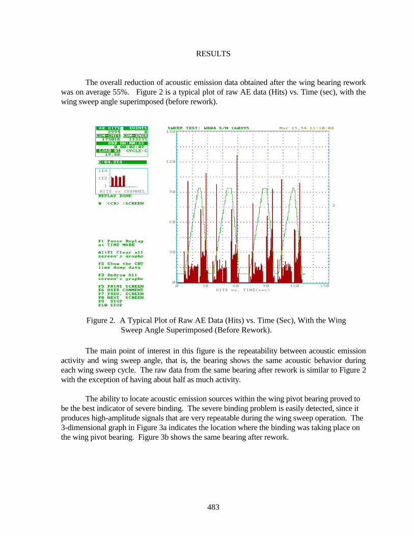
483
RESULTS
The overall reduction of acoustic emission data obtained after the wing bearing reworkwas on average 55%. Figure 2 is a typical plot of raw AE data (Hits) vs. Time (sec), with thewing sweep angle superimposed (before rework).
The main point of interest in this figure is the repeatability between acoustic emissionactivity and wing sweep angle, that is, the bearing shows the same acoustic behavior duringeach wing sweep cycle. The raw data from the same bearing after rework is similar to Figure 2with the exception of having about half as much activity.
The ability to locate acoustic emission sources within the wing pivot bearing proved tobe the best indicator of severe binding. The severe binding problem is easily detected, since itproduces high-amplitude signals that are very repeatable during the wing sweep operation. The3-dimensional graph in Figure 3a indicates the location where the binding was taking place onthe wing pivot bearing. Figure 3b shows the same bearing after rework.
Figure 2. A Typical Plot of Raw AE Data (Hits) vs. Time (Sec), With the WingSweep Angle Superimposed (Before Rework).
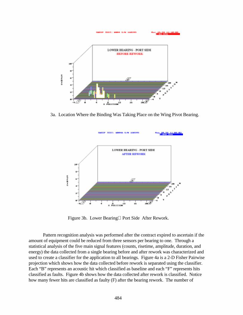
484
Pattern recognition analysis was performed after the contract expired to ascertain if theamount of equipment could be reduced from three sensors per bearing to one. Through astatistical analysis of the five main signal features (counts, risetime, amplitude, duration, andenergy) the data collected from a single bearing before and after rework was characterized andused to create a classifier for the application to all bearings. Figure 4a is a 2-D Fisher Pairwiseprojection which shows how the data collected before rework is separated using the classifier. Each “B” represents an acoustic hit which classified as baseline and each “F” represents hitsclassified as faults. Figure 4b shows how the data collected after rework is classified. Noticehow many fewer hits are classified as faulty (F) after the bearing rework. The number of
Figure 3b. Lower BearingPort Side After Rework.
3a. Location Where the Binding Was Taking Place on the Wing Pivot Bearing.
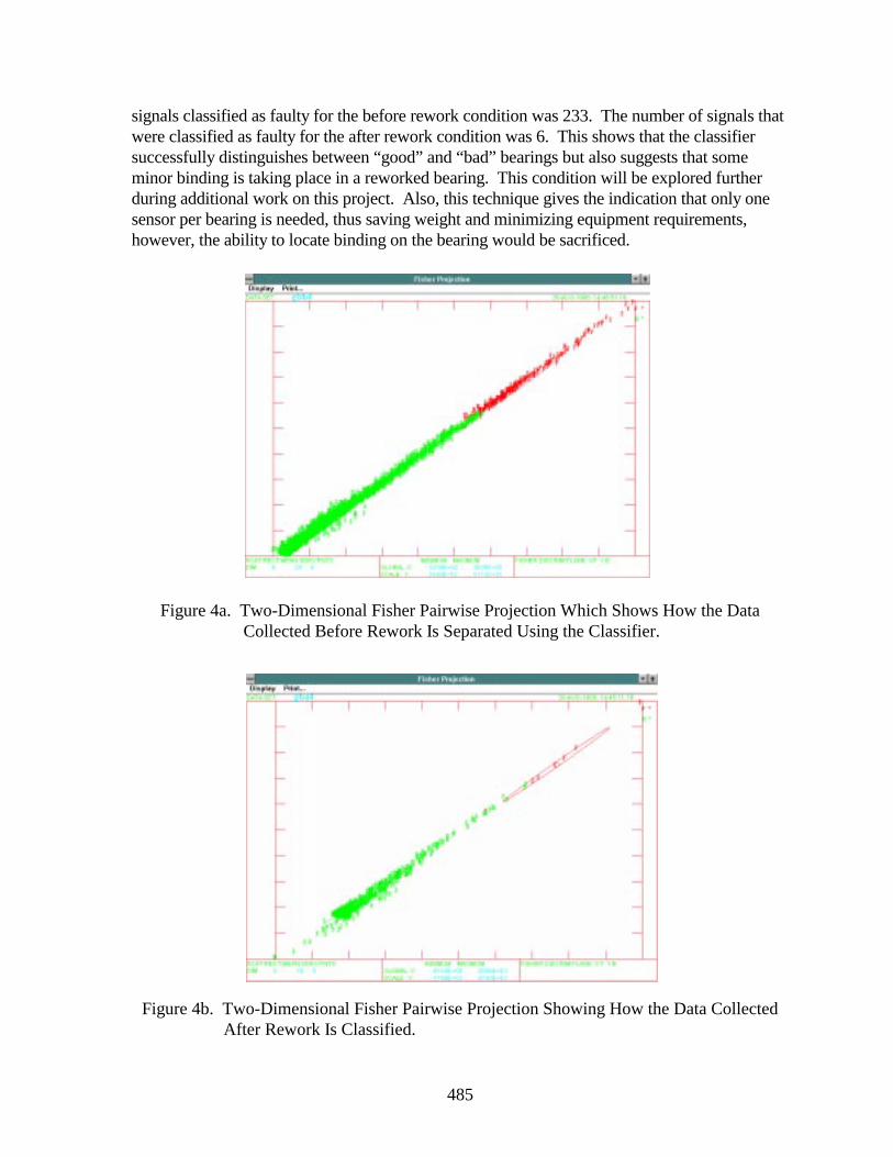
485
signals classified as faulty for the before rework condition was 233. The number of signals thatwere classified as faulty for the after rework condition was 6. This shows that the classifiersuccessfully distinguishes between “good” and “bad” bearings but also suggests that someminor binding is taking place in a reworked bearing. This condition will be explored furtherduring additional work on this project. Also, this technique gives the indication that only onesensor per bearing is needed, thus saving weight and minimizing equipment requirements,however, the ability to locate binding on the bearing would be sacrificed.
Figure 4a. Two-Dimensional Fisher Pairwise Projection Which Shows How the DataCollected Before Rework Is Separated Using the Classifier.
Figure 4b. Two-Dimensional Fisher Pairwise Projection Showing How the Data CollectedAfter Rework Is Classified.

486
CONCLUSIONS
1. The feasibility of using acoustic emission nondestructive testing methods has beenestablished for the in situ inspection of Navy F-14 aircraft wing pivot bearings.
2. There is a substantial reduction in the amount of acoustic emission activity after rework. 3. Severe binding in two bearings was detected and located using the acoustic emission
approach. 4. The application of signal pattern recognition analysis techniques shows promise in
reducing the amount of instrumentation and weight for an in-flight bearing monitor.
487
OPERATOR CONCERNS ABOUT WIDESPREAD FATIGUE DAMAGE ANDHOW IT MAY BE HANDLED AND REGULATED IN THE
COMMERCIAL ENVIRONMENT
David V. FinchConsultant
Windsor, SL4 5ER, England
SUMMARY
The paper compares the theory and practice of aircraft structural maintenance andinspection in the current damage tolerant regime and how this may need to change in thepresence of widespread fatigue damage. Aspects considered include the regulatory role,operator feedback, maintenance program development and whether widespread fatiguedamage (WFD) means a return to safe life. Particular reference is made to the need foradvice, support and training which is the principle professional interest of the author.
DEFINITIONS
Words and phrases printed in bold italic type are defined in Appendix C - Glossary.When subsequently used in the text these words and others having a specific meaning inaviation are printed in italics.
INTRODUCTION
Fail-safe and damage tolerance design together with inspections of appropriate frequency and focus have successfully safeguarded the structural integrity of public transportaircraft over the last 28 years. Models certified during this time and earlier have been subjectto extensive structural analysis and testing leading to the specification of directed inspectionssearching for the initial indications of fatigue damage. Fatigue cracking in service, however,has frequently differed from that predicted by test or analysis [Ref. 1] and potentiallycatastrophic conditions have not always been found by scheduled inspection. In someinstances failure has only been evident at a very advanced stage through malfuncion or bychance observation.
Some of these failures have resulted from multiple-site damage (MSD) and multipleelement damage (MED) [See Figure 1]. The Manufacturing and regulatory sectors of theindustry have been aware of these phenomena for many years [Ref. 2] and of the limitedability of the fail-safe features built into current designs to contain widely distributed cracking[Ref. 3].
488
Damage tolerance rules require consideration of damage at multiple sites [seeFAR/JAR 25.571(b)] but widespread fatigue damage (WFD) reduces the probability thatcritical conditions will be found during routine work or will be revealed, prior to completefailure, by obvious and safe malfunction.
The potential immediacy of WFD is shown by the summary of service and fatigue testdata for the 11 models overseen by the Airworthiness Assurance Working Group (AAWG)[see Appendix B]. Many other tests and inspections including the teardown of aircraft retiredfrom service have been carried out to substantiate freedom from WFD but the table doesindicate that some aircraft, those with the highest number of flight cycles relative to theservice life objectives and full-scale fatigue test experience, are entering the phase where WFDmay be present.
All the major manufacturers are evaluating their aircraft for WFD in the critical areasof the wing, empenage, and pressure fuselage i.a.w. guidelines provided through the AviationRulemaking Advisory Committee (ARAC) and the AAWG [Refs. 1 and 4]. Where WFD isforecast, more frequent and more intensive inspections, modifications, or life limits may berequired. There may be additional criteria for repair and further constraints on maintenanceprogram development.
Operators need to be aware that, for some of the oldest aircraft, the days of“Tolerance to Damage” and “Unlimited Life” may be numbered. This paper considers thecontribution that airlines can make to the orderly and economic management of the WFDphenomena.
DAMAGE TOLERANT INSPECTION
Figure 2 shows how a structural item may be weakened by the combined effects offatigue and other damage until final failure occurs at “F.”
“M” is the minimum detectable flaw sizeUltimate strength is lost at “U.”At “L” the item can no longer support Limit Load.
To meet damage tolerance rules failure must be detected prior to “L.” Area “MXL”represents a combination of defect size and time available for detection and may be regardedas the window for damage tolerant inspection.
To ensure adequate opportunity to detect deterioration fail-safe features, frames,stringers, and doublers are incorporated to arrest crack growth and to extend the inspectionwindow. Compare MX1L1 and MX2L2 in Figure 3.
489
The inspection program that can then be applied is illustrated in Figure 4.
When a problem or potential problem has been identified, Detail or Special Detailinspections can be specified in which the Inspector’s attention is directed very precisely to thesubject feature. Special detail inspections may be used to find very small and inaccessibleflaws but their area of search is limited and techniques must be tailored to the particular formof the potential defect. It is neither economic nor practical to survey the whole aircraft in thisway.
General visual inspections cannot be expected to find small defects but serve toidentify problems that, once known, may be more effectively controlled by detail or specialdetail inspections or terminated by modification.
In the figure the vertical distance between design strength and the horizontal barsrepresenting the inspection levels indicates the minimum defect size that can be detected. Theposition and spacing of the vertical bars indicates the timing and frequency of inspection.
• Inspections which can detect deterioration before final failure are shown in solid black.The probability of damage detection increases with the vertical length of the solid bar.
• Inspections which are unlikely to find a defect because they are performed either too
early or too late are shown by a shaded vertical bar.
If deterioration is not found by inspection then the fail-safe features of the design maywell ensure that the structure continues to carry the applied loads until the condition becomesapparent during servicing or preflight checks or is revealed by malfunction, typically by fuelleaks from the wing or difficulty in pressurizing the fuselage.
The fact that serious structural defects have been found and, on occasion, continue tobe found in this way on aircraft operated by some of the most sophisticated airlines in theworld indicates that:
• Damage tolerant standards, as currently interpreted, are not over generous.
The fact, also, that these events now very rarely feature in the accident statistics shows:
• • The importance of Fail-safe.
INSPECTION WITH WFD
Figure 5 illustrates the classic case of cracking in the longitudinal joints of a fuselageskin when multiple site damage is present and widespread:

490
• For both detail and general inspections the total crack length at detection is the sumof all the adjacent individual cracks; i.e., there can be a significant reduction in residualstrength prior to detection.
• If MSD is sufficiently invasive, then, regardless of whether frames and doublers are
intact, there is little to prevent the formation of a continuous multiple bay crack.
The effects are shown in Figure 6.
• The inspection window, if it still exists at all, is now much smaller than before. Cf.Figure 4.
• The possibility that catastrophic failure will be averted by evident damage prior to
departure or by safe malfunction is greatly diminished. The fail-safe features areineffective and deterioration through crack coalescence can be precipitously steep.
If Figure 6 comes close to representing the situation with WFD it would be difficult toclaim that damage tolerant criteria per FAR/JAR 25.571 can be satisfied. The alternative issafe life.
SAFE LIFE
Figure 7 illustrates both the principle and the inherent weakness of the safe lifephilosophy.
Safe life attempts to control condition (strength) on the vertical scale by limiting life(flight cycles) along the horizontal scale and assumes a known relationship between theseparameters.
Catherine Bigelow, speaking to the Sixth FAA-NASA International Conference on theContinued Airworthiness of Aircraft Structures [Ref. 5], listed 12 areas of uncertainty in theprediction of WFD.
Accidental damage incurred during manufacture or installation, a variable notspecifically mentioned by Catherine, led to the failure of a Viscount wing spar over WesternAustralia after 8,090 flights [Ref. 6]. The approved safe life was 11,400 flights. Though theaccident occurred nearly 28 years ago it still provides a classic illustration of the vulnerabilityof the safe life concept.
Testing and analytical techniques have improved immeasurably since 1968 and are stillbeing developed. Some 28 of the papers presented at this Symposium are, by the author’sestimation, concerned with fatigue life prediction or risk analysis.
491
• Is it now possible, by these methods alone, to resolve the uncertainties and to establishsafe lives which will offer protection against WFD and also satisfy reasonableeconomic criteria?
• Do the manufacturers and regulatory authorities wish to take responsibility for setting
inspection thresholds and/or life limits without the fullest possible reference to serviceexperience?
• Do operators wish to participate in a managed approach to the identification of WFD
and, if so, do they understand the task and are they prepared for it?
OPERATOR ATTITUDES
A problem in the past may have been that damage tolerant designs were too good.Serviceability was excellent, major incidents were few, complacency was not penalized, and itseemed that the aircraft structure could be left to look after itself.
In 1988 Boeing Maintenance Survey Teams which at that time had visited 44operators over all five continents and witnessed major maintenance on 80 high-time aircraft,had to report that:
• Maintenance programs generally did not recognize the significance of aircraft age • A few aircraft had improper modifications or repairs and some required extensive
repairs for corrosion • The condition of some aircraft reflected a reduction in operator’s engineering and
maintenance staffs [Ref. 7].
Contemporary comments by McDonnell Douglas support teams were broadly similar,adding that:
• Maintenance standards were generally below expectation, some below fail saferequirements [Ref. 4].
Have things changed in the post-Aloha world? Boeing and McDonnell Douglas reportthat it has. Both have continued their surveys and the total Boeing study now includes 97operators and 190 aircraft. Both now comment to the effect that:
• Airlines are doing a better job in maintaining their aircraft and have an increasedawareness of structural issues and sound maintenance practices.
492
Indeed, it would be remarkable if it were otherwise given all the aging aircraft activityof the past 8 years.
How can this awareness be sustained and enhanced to permit a successful managedapproach to the problem of WFD - assuming that airlines do wish to participate in thisactivity?
DEVELOPMENT IN SERVICE
Figure 8 provides a further illustration of the current damage tolerant approach inwhich a minimum standard of structural strength is maintained directly by inspection.
A rising incidence of in-service defect findings will indicate the need for enhancedinspection or termination at some level “R” determined by the economic penalty or risk toairworthiness of continuing with inspection and repair. In a well managed program theoperator will evaluate the data and use his judgment to initiate such action though theregulator may intervene on safety grounds.
The process had been likened to “Listening and responding to what the aircraft istelling you.”
Though it eliminates many of the uncertainties associated with the control ofairworthiness by safe life, damage tolerant inspection is crucially dependent on the standardsof the operator and the performance of his inspection staff - with all their human andorganizational frailties.
It is therefore appropriate to consider the role, status, and training of the inspector andthe ethos of the organization in which he or she works.
INSPECTION
The inspection task may be expressed as: The examination of an item, assembly, orsystem for condition or functioning in conformity to a defined standard.
While this may be true for directed inspections aimed at well defined problems it is agross oversimplification of the observations and judgments made by an inspector performingthe more general inspections which are most likely to reveal new or unquantified defects.
Figure 9 illustrates the nature of the decisions that the inspector has to take [see alsoFigure 3]:
493
• Is ultimate strength or functional capability retained? (i.e., Conditions 1.3. orCondition 4.)
• How rapid is the rate of deterioration and when must rectification be implemented? • Does this represent a potentially hazardous condition which should be reported?
Inspectors generally understand and accept their responsibility for immediateairworthiness and perform this role conscientiously and well, taking appropriate account ofoperational demands and practical constraints. The task and responsibility reflect theirexperience and culture and it is to this end that training has been largely directed. They areless familiar with the more strategic role in which the aircraft may be regarded as a flying testarticle and they are part of a research team dedicated to extracting optimum performance.
Figure 10 illustrates how the system should work concentrating on the role of theinspector and the factors that shape his or her performance.
IDENTIFICATION OF WFD
Deficiencies in the system are relatively benign within the damage tolerant envelope.If an operator fails to recognize and evaluate a problem the inspection/maintenance programwill not be as well tuned as it could be but airworthiness is not immediately at risk. For thereasons outlined in Section 3 the whole process is much more critical in the presence of WFDand a proper understanding of the operator’s investigative role is essential if serviceexperience is to be applied successfully to the determination of WFD maintenance policy.
The objective, illustrated in Figure 11, is:
• To position the safe life barrier as far, but no further, to the left than necessary toensure that the risk “R” of catastrophic failure through WFD is extremely small.
• To determine what additional inspections “B” and/or other maintenance requirements
are necessary to ensure safe operation prior to the imposition of a life limit.
The task of the inspector and the whole of the operator’s research team is torecognize and report the first indications of MSD/MED and to investigate whether this iswidespread.
Figure 1 provides an example of this task and the possible impact on a maintenancecheck.
494
The Figure shows cracks in three adjacent stringer end fittings. The aircraft could berepaired and returned to service simply by replacing the fittings but such MED, if widespread,could be potentially catastrophic.
Operator Action - Recognize the condition and report findings. Check other aircrafton maintenance and report on the condition of similar fittings, where accessible.
Possible Consequences - A Telegraphic AD to inspect fittings on all high-cycleaircraft. A life limit on fittings if integrity cannot be maintained by inspection.
A further example featuring MSD is given in the Repair Case Study (Appendix A).
INFORMATION, TRAINING AND TECHNICAL SUPPORT
It has been claimed that very few people in the industry understand the WFD condition[Ref. 3] and if this is the case there is a need for innovation and training at all levels to ensurecommitment to, and proper implementation of, a participatory program as outlined in theprevious section.
Advice is available to customers from the manufacturers. For example:
• Boeing offers structural integrity awareness material and training for engineers inrepair design, provide integrated maintenance programs for aging aircraft, and alsohost structural conferences around the world.
• McDonnell Douglas offers aging aircraft program training to operators [Ref. 4].
Other opportunities include Structures Task Group (STG) meetings to which LockheedMartin, for example, invites all L-1011 operators.
These initiatives are well supported but attendance is voluntary and the message doesnot necessarily reach to the executive level at which airline maintenance policy is determinedor to those who work on the shop floor.
The recognition and assessment of structural deterioration is only one of many aspectsin the requirements for the licensing and approval of aircraft inspectors and only one of manytasks that he or she may be required to undertake. The appropriate interpretation and actionin the case of some findings may therefore be beyond the scope of the inspector and enter therealm of the structural engineer. It follows that a structural engineer should be available toadvise and direct this activity, but it is the inspector who comes face to face with the aircraftand who must appreciate the need to alert the engineer to a potentially dangerous condition.

495
Some specific training for inspectors engaged in the maintenance of elderly aircraft,possibly in the form of a workshop in which experience can be shared, is therefore indicated.
Material for such workshops has been developed by the author, some of which isshown in the figures used to illustrate this paper.
Ad hoc attempts to develop and correlate inspection skills have also been made bysome operators in the United States but such initiatives do not, as yet, form a part of anyrequired training curriculum.
THE ROLE OF DIRECTIVES
Although the inflexibility of directives make them unsuited to the investigative work asdescribed in the paragraphs on DEVELOPMENT IN SERVICE and IDENTIFICATION OFWFD directives do have a role:
• They ensure attention to known problems. • They can raise awareness. The improved standards noted by McDonnell Douglas and
Boeing can, in part, be attributed to the mandating of programs such as the corrosionprevention and control programs (CPCP).
A proliferation of ADs can also encourage the perception that anything critical toairworthiness will be so covered. In discussing the regulation of aircraft structuralmaintenance programs, David Lotterer (ATA), playing devil’s advocate, [Ref. 8] expressedthis belief in the question:
“If, from a business perspective, the FAA ACOs and the AD process will take care ofyour airworthiness issues, why do you need all those structures engineers at theairlines?”
Clearly, this approach is the very antithesis of that required for the identification andappropriate reporting of MSD/MED in service as discussed in this paper [SeeIDENTIFICATION OF WFD].
THE COMMERCIAL ENVIRONMENT
It would be unwise to assume that the favorable trends noted by Boeing andMcDonnell Douglas will continue without some regulatory incentives. Avowals of “Safety isParamount” notwithstanding, airlines and airline maintenance management will be driven, in
496
an increasingly competitive environment, by the most tangible of economic and legal criteria,i.e.,
• Budgets• On time delivery• Operational reliability• Compliance with legislation
Maintenance will increasingly be contracted to facilities offering the lowest costs andthe shortest, guaranteed delivery times. The quality of work may not be inferior but theeconomic imperatives and potential reduction in technical continuity are unlikely to befavorable to an understanding and the effective reporting of WFD.
Though highly resistant to accepting conservative safe lives or the early imposition ofextensive and frequent special inspections [Ref. 9], operators may yet fail to fully embrace theparticipatory and investigative role and organizational commitment outlined in the paragraphson IDENTIFICATION OF WFD and INFORMATION, TRAINING AND TECHNICALSUPPORT unless this is supported by some legislation.
THE WAY AHEAD
The key to progress may lie in the words of John Chaplin, former Head of the CAAAirworthiness Division. Speaking at the Royal Aeronautical Society in London in 1980 hesaid:
“Airworthiness cannot be achieved by regulation (alone). Regulation can establisha framework within which all who are concerned with the design, construction, andoperation of aircraft can work and can set boundaries of responsible behavior.”
For the approval of organizations for structural work on aging aircraft it may beappropriate to require enhanced standards of management, organization, and technicaloversight. For example:
• Production engineering staff to translate operating rules, Ads, and manufacturer’sprograms and bulletins into practical working instructions and control documents foruse on the shop floor.
• Qualified technical or engineering staff who are familiar with the principles of
structural airworthiness including the possible interaction of accidental, environmental,and fatigue damage, and who understand the requirements for corrosion control andthe critical nature of WFD.
497
• Inspection and maintenance staff who have received general and model specifictraining in structural inspection practices and techniques, defect investigation andreporting, and have practical experience of structural inspection with an approvedorganization.
• Facilities, equipment, and resources necessary for the effective inspection of critical
features of the aircraft structure. • Effective reporting channels to the manufacturer and appropriate regulatory authority,
functioning to their satisfaction. • Maintenance contracts that provide for structural abnormalities to be effectively
investigated, whether or not such work is originally scheduled. • Quality oversight to ensure that the airworthiness intentions of these provisions are
being achieved.
The above list is not exhaustive but does indicate the type of approach which may be effectivein ensuring the proper detection, investigations, and reporting of WFD and other structuralabnormalities of potential airworthiness concern.
Some may argue that all these good things are required and happen already. If that istrue then we do not have a problem. If there are deficiencies, the authorities, manufacturers,and operators alike may wish to consider the case as outlined in this paper for some legalreinforcement to the three legged stool and to responsible behavior.
Such action would present no difficulty to many engineering and maintenanceorganizations as currently established. Others may have to upgrade if they wish to meet thecriteria and to undertake structural work on aging airplanes.
CONCLUSIONS
1) Despite extensive fatigue testing, tear down evaluations, and the sophisticatedanalytical techniques now used by the manufacturers, service experience still providesthe first and most reliable indication of many structural problems and potentiallycatastrophic failures.
2) Widespread fatigue damage significantly reduces the opportunity to safely detect damage
by inspection or general alertness and the probability that a malfunction will be safe. 3) Operation to the threshold of the WFD regime demands a heightened awareness by
maintenance and engineering managers of the principles underlying structuralairworthiness and may require specific training for inspection and maintenance staff.
498
4) Additional maintenance approval requirements may be necessary for the safe operationand maintenance of aircraft susceptible to WFD.
REFERENCES
1. Hidano, Lance A. and Goranson, Ulf G.: Inspection Programs for DamageToleranceMeeting the Regulatory Challenge. Proceedings of the FAA-NASA SixthInternational Conference on Continued Airworthiness of Aircraft Structures,DOT/FAA/AR-95/86, December 1995.
2. Maxwell, R. D. J.: RAE Farnborough, Fail Safe Philosophy: An Introduction to the
Symposium. 7th. ICAF., London, TR73183, 1973. 3. Swift, Tom: WFD. Monitoring - Issues and Concerns, 5th. ICCAAS, Hamburg,
DGLR-Bericht 93-02, 1993. 4. Billson, Margaret S.: Air Safety - Our Most Important Product as a Manufacturer.
Proceedings of the FAA-NASA Sixth International Conference on ContinuedAirworthiness of Aircraft Structures, DOT/FAA/AR-95/86, December 1995.
5. Bigelow, Catherine A. and Tan, Paul W.: An Integrated Methodology for Assessing
WFD in Aircraft Structures. Proceedings of the FAA-NASA Sixth InternationalConference on Continued Airworthiness of Aircraft Structures, DOT/FAA/AR-95/86,December 1995.
6. Viscount 720C VH-RMQ Mac Robertson Miller PTY Commonwealth of Australia
Department of Civil Aviation Accident Investigation Report, Sept. 1969. 7. Boeing Aging Aircraft Conference - 1988. TE 41559 8-29-88. 8. Lotterer, David: Regulations Affecting Air Carrier Structural Inspection Programs.
Proceedings of the FAA-NASA Sixth International Conference on ContinuedAirworthiness of Aircraft Structures, DOT/FAA/AR-95/86, December 1995.
9. McBride, Tony: Managed or Mandated Maintenance ProgramsA Growing
Concern. Proceedings of the FAA-NASA Sixth International Conference onContinued Airworthiness of Aircraft Structures, DOT/FAA/AR-95/86, December1995.
10. Swift, Tom: Repairs to Damage Tolerant Aircraft. SIAA. Int. Symposium. FAA-
AIR-90-01), Atlanta, 1990
499
APPENDIX ACASE STUDY
Figure 12 shows an external patch repair of a fuselage skin for corrosion and cracking(D) along a stringer line.
Cracking which developed in the skin along the outer row of fasteners (Section AA) ishidden externally by the patch and internally by the stringer and could extend over a length (L)of more than two frame bays before it was detected by external inspection [Ref. 10].
Undetected cracking under the patch would also degrade the ability of the structure tosurvive adjacent foreign object damage. The repair does not meet damage tolerant criteriaand would be classified as Category C - Temporary.
The scheme could be improved by extending the patch to line X. This moves thecritical skin location to a line of new noncountersunk holes where crack initiation is less likelyand cracking could be seen internally. The repair would have a longer life but would still betemporary.
A more immediate concern arises if the repair is applied to a very high-cycle aircraft.The cracking may result not from the corrosion but from MSD coalescence and other smallundetected cracks may exist outside the boundaries of the proposed repair [See Figs. 1 and 6].
An appropriate operator action in this case would be:
• Recognize the possibility of MSD. • Remove extra fasteners and check hole bores for cracks using a high frequency eddy-
current probe. • If no cracks are found, cold work hole bores to inhibit undetected damage and
complete a temporary repair. • If additional cracking is found report the condition.
Possible consequences of finding and reporting cracks are:
• On the subject aircraft, a much more extensive repair than originally proposed andpossibly a skin change.
• An AD for special detail inspections at all skin attachment hole locations in the
suspect area on all aircraft over the inspection threshold.
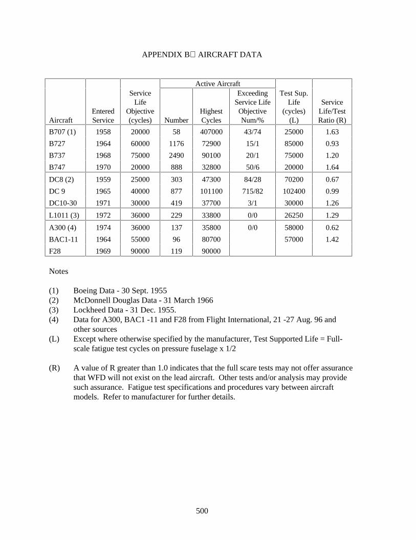
500
APPENDIX BAIRCRAFT DATA
Active Aircraft
AircraftEnteredService
ServiceLife
Objective(cycles) Number
HighestCycles
ExceedingService LifeObjectiveNum/%
Test Sup.Life
(cycles)(L)
ServiceLife/TestRatio (R)
B707 (1) 1958 20000 58 407000 43/74 25000 1.63
B727 1964 60000 1176 72900 15/1 85000 0.93
B737 1968 75000 2490 90100 20/1 75000 1.20
B747 1970 20000 888 32800 50/6 20000 1.64
DC8 (2) 1959 25000 303 47300 84/28 70200 0.67
DC 9 1965 40000 877 101100 715/82 102400 0.99
DC10-30 1971 30000 419 37700 3/1 30000 1.26
L1011 (3) 1972 36000 229 33800 0/0 26250 1.29
A300 (4) 1974 36000 137 35800 0/0 58000 0.62
BAC1-11 1964 55000 96 80700 57000 1.42
F28 1969 90000 119 90000
Notes
(1) Boeing Data - 30 Sept. 1955(2) McDonnell Douglas Data - 31 March 1966(3) Lockheed Data - 31 Dec. 1955.(4) Data for A300, BAC1 -11 and F28 from Flight International, 21 -27 Aug. 96 and
other sources(L) Except where otherwise specified by the manufacturer, Test Supported Life = Full-
scale fatigue test cycles on pressure fuselage x 1/2
(R) A value of R greater than 1.0 indicates that the full scare tests may not offer assurancethat WFD will not exist on the lead aircraft. Other tests and/or analysis may providesuch assurance. Fatigue test specifications and procedures vary between aircraftmodels. Refer to manufacturer for further details.

501
APPENDIX CGLOSSARY
The following definitions refer to the meaning of words and phrases as used in this paper.Other definitions may be found in other documentation.
Airworthiness - The ability of an airplane to complete a flight safely while operatinganywhere within the fail-safe design envelope.
Airworthiness Assurance Working Group - A high-level industry steering committeeformed to oversee the work of Structures Task Groups - Manufacturers’ structuralspecialists, airline engineers, and regulatory authority representatives.
Damage Tolerance - The ability of structure to sustain anticipated loads in the presence ofdamage until such damage is detected by inspection or safe malfunction and repaired.
Directed Inspection - A scheduled inspection specified in the operator’s maintenanceprogram or in a service bulletin in which the attention of the inspector is directed to aparticular item, component, assembly, or feature.
Engineering - That part of the organization staffed by professionally qualified engineersresponsible for standards and procedures, the inspection schedule, inspection programdevelopment, specification of aircraft modifications, technical support to maintenanceand design liaison with manufacturers, and the regulatory authority.
Failure - The inability of an item to perform within previously specified limits.
Fail-Safe
Design - A design which will permit continued operation of an airplane for a limitedperiod after a failure in service.
Structure - The ability of damaged structure to withstand an infrequent high load.
Fatigue Damage
Multiple Element - The simultaneous cracking of multiple load path discrete elementsworking at similar stress levels.
Multiple Site - The presence of a number of adjacent small cracks that might coalesce toform a single long crack.
Widespread - The simultaneous presence of cracks at multiple structural details of suchsize and density that the structure will no longer meet Damage Tolerancerequirements.
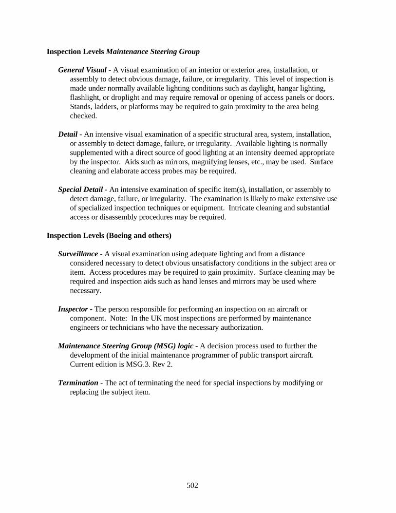
502
Inspection Levels Maintenance Steering Group
General Visual - A visual examination of an interior or exterior area, installation, orassembly to detect obvious damage, failure, or irregularity. This level of inspection ismade under normally available lighting conditions such as daylight, hangar lighting,flashlight, or droplight and may require removal or opening of access panels or doors.Stands, ladders, or platforms may be required to gain proximity to the area beingchecked.
Detail - An intensive visual examination of a specific structural area, system, installation,or assembly to detect damage, failure, or irregularity. Available lighting is normallysupplemented with a direct source of good lighting at an intensity deemed appropriateby the inspector. Aids such as mirrors, magnifying lenses, etc., may be used. Surfacecleaning and elaborate access probes may be required.
Special Detail - An intensive examination of specific item(s), installation, or assembly todetect damage, failure, or irregularity. The examination is likely to make extensive useof specialized inspection techniques or equipment. Intricate cleaning and substantialaccess or disassembly procedures may be required.
Inspection Levels (Boeing and others)
Surveillance - A visual examination using adequate lighting and from a distanceconsidered necessary to detect obvious unsatisfactory conditions in the subject area oritem. Access procedures may be required to gain proximity. Surface cleaning may berequired and inspection aids such as hand lenses and mirrors may be used wherenecessary.
Inspector - The person responsible for performing an inspection on an aircraft orcomponent. Note: In the UK most inspections are performed by maintenanceengineers or technicians who have the necessary authorization.
Maintenance Steering Group (MSG) logic - A decision process used to further thedevelopment of the initial maintenance programmer of public transport aircraft.Current edition is MSG.3. Rev 2.
Termination - The act of terminating the need for special inspections by modifying orreplacing the subject item.
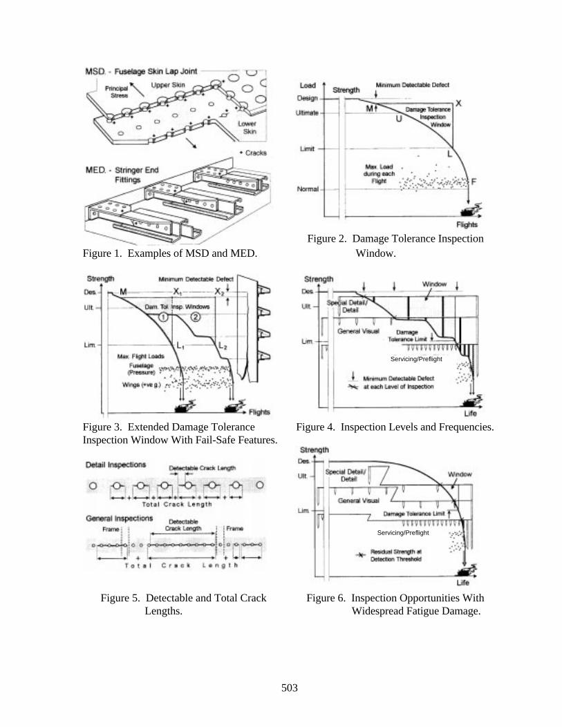
503
Figure 2. Damage Tolerance InspectionFigure 1. Examples of MSD and MED. Window.
Figure 3. Extended Damage ToleranceInspection Window With Fail-Safe Features.
Figure 4. Inspection Levels and Frequencies.
Figure 5. Detectable and Total CrackLengths.
Figure 6. Inspection Opportunities WithWidespread Fatigue Damage.
Servicing/Preflight
Servicing/Preflight
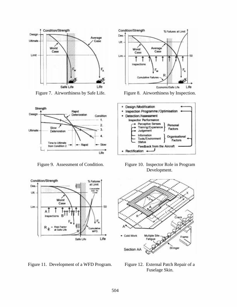
504
Figure 7. Airworthiness by Safe Life. Figure 8. Airworthiness by Inspection.
Figure 9. Assessment of Condition. Figure 10. Inspector Role in ProgramDevelopment.
Figure 11. Development of a WFD Program. Figure 12. External Patch Repair of aFuselage Skin.
505
PREDICTIONS O F STABLE GROWTH O F A LEAD CRACK ANDMULTI PLE-SITE DAMAGE USING ELASTIC- PLASTIC
FINITE ELEMENT METHOD (E PFEM) AND ELASTIC- PLASTICFINITE ELEMENT ALTERNATING METHOD (E PFEAM)
L. Wang, F. W. Brust, and S. N. AtluriFAA Center of Excellence for
Computational Modeling of Aircraft StructuresGeorgia Institute of TechnologyAtlanta, Georgia 30332-0356
SUMMARY
Damage tolerance analyses of an aging aircraft require numerical simulations of stabletearing of the skin of the aircraft. This paper presents a methodology for the analyses ofmultiple-site damage (MSD) in the presence of a lead crack, based on the T*-integral fractureparameter and the finite element alternating method. In the proposed methodology, the T*-resistance curve is obtained from the numerical simulations in the generation phase analysesof experiments of center-cracked panels containing single cracks. The computed T*-resistance curve is then used in numerical predictions of stable tearing of the aircraft skin inthe application phase analyses. To validate this methodology, generation phase analyses andapplication phase analyses are performed for the MSD tests performed at the NationalInstitute of Standards and Technology (NIST). Numerical results show that a single T*-resistance curve can be obtained from the tearing of center-cracked panels of different sizes,and the single T*-resistance curve can be used to predict the stable tearing of the lead cracksand their linkup with MSD cracks in front of them. The predicted curves of load versus crackextension are in good agreement with the experimental measurements obtained at NIST.Through these numerical analyses and comparisons, this paper presents, for the first time, atruly validated energy based fracture criterion for the analysis of stable growth and linkup ofmultiple cracks in an MSD situation.
INTRODUCTION
Practical methods for predicting the residual strength of multiple-site damage (MSD)problems include the plastic zone method [1], the crack tip opening angle (CTOA) method[2], and the T*-integral method [3, 4, 5, 6, 7]. As a simple engineering approach, the plasticzone method assumes that the main crack will link with the MSD crack ahead of it if theirplastic zones overlap. The plastic zones are estimated using an elastic analogy such as anIrwin estimation. Since it is difficult to evaluate the effect of MSD cracks and the effect ofplastic hardening within such a framework, significant errors can occur. Furthermore, when
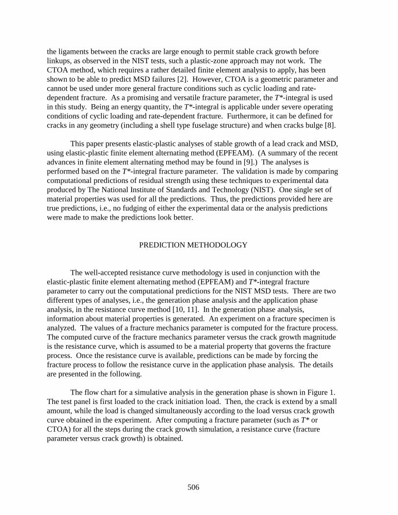
506
the ligaments between the cracks are large enough to permit stable crack growth beforelinkups, as observed in the NIST tests, such a plastic-zone approach may not work. TheCTOA method, which requires a rather detailed finite element analysis to apply, has beenshown to be able to predict MSD failures [2]. However, CTOA is a geometric parameter andcannot be used under more general fracture conditions such as cyclic loading and rate-dependent fracture. As a promising and versatile fracture parameter, the T*-integral is usedin this study. Being an energy quantity, the T*-integral is applicable under severe operatingconditions of cyclic loading and rate-dependent fracture. Furthermore, it can be defined forcracks in any geometry (including a shell type fuselage structure) and when cracks bulge [8].
This paper presents elastic-plastic analyses of stable growth of a lead crack and MSD,using elastic-plastic finite element alternating method (EPFEAM). (A summary of the recentadvances in finite element alternating method may be found in [9].) The analyses isperformed based on the T*-integral fracture parameter. The validation is made by comparingcomputational predictions of residual strength using these techniques to experimental dataproduced by The National Institute of Standards and Technology (NIST). One single set ofmaterial properties was used for all the predictions. Thus, the predictions provided here aretrue predictions, i.e., no fudging of either the experimental data or the analysis predictionswere made to make the predictions look better.
PREDICTION METHODOLOGY
The well-accepted resistance curve methodology is used in conjunction with theelastic-plastic finite element alternating method (EPFEAM) and T*-integral fractureparameter to carry out the computational predictions for the NIST MSD tests. There are twodifferent types of analyses, i.e., the generation phase analysis and the application phaseanalysis, in the resistance curve method [10, 11]. In the generation phase analysis,information about material properties is generated. An experiment on a fracture specimen isanalyzed. The values of a fracture mechanics parameter is computed for the fracture process.The computed curve of the fracture mechanics parameter versus the crack growth magnitudeis the resistance curve, which is assumed to be a material property that governs the fractureprocess. Once the resistance curve is available, predictions can be made by forcing thefracture process to follow the resistance curve in the application phase analysis. The detailsare presented in the following.
The flow chart for a simulative analysis in the generation phase is shown in Figure 1.The test panel is first loaded to the crack initiation load. Then, the crack is extend by a smallamount, while the load is changed simultaneously according to the load versus crack growthcurve obtained in the experiment. After computing a fracture parameter (such as T* orCTOA) for all the steps during the crack growth simulation, a resistance curve (fractureparameter versus crack growth) is obtained.
507
The generation phase analyses of test data to develop a resistance curve are usuallyperformed when obtaining the curve directly from the test, which is time consuming,expensive, and impractical. It should be noted that both CTOA [2] and T* [12] resistancecurves can and have been obtained directly from experiments. But doing so is not necessary.
In a predictive analysis in the application phase, the crack extension is controlled bythe T*-resistance curve. A flow chart for the application phase is shown in Figure 2. It isassumed that 1) an increase in load (displacement) at the far field will increase the T* value atthe crack tip; 2) any crack extension will decrease the T* value; and 3) the T*-resistancecurve does not decrease as the crack extends. Under these conditions, the simple predictivealgorithm in Figure 2 can be used.
NIST MULTIPLE SITE DAMAGE EXPERIMENTS
Figures 3 and 4 summarize the series of tests carried out at NIST. More details onthese tests can be found in [14]. The specimens were made of 2024-T3 aluminum, 90 incheswide, 150 inches high, 0.04 inch thick, with the lead crack located at the center of the panel.The definition parameters of MSD cracks, such as the MSD crack spacing, sMSD, etc., aredefined graphically in Figure 3. The MSD cracks were equally spaced. The specimens weresymmetric about their horizontal and vertical centerlines.
The cracks were introduced by a series of saw cuts. The crack tips were made by thesharpest jeweler’s saw available, having a tip radius of 0.003 inch. To simulate cracksemanating from rivet holes as occurs in an aircraft fuselage, the MSD cracks were cut from0.22-inch holes that were drilled into the sheets before the saw cuts were made. Saw cuts caninduce plastic deformations near the crack tips. However, this effect was not considered inthis study. In addition, antibuckling guides were used in all tests, except for the MSD-6, sothat the specimens did not buckle out of plane due to the small thickness. The test procedureconsisted of pulling the specimen to fracture under displacement control. Both tips of themain crack did not grow at the same loads in the test due to imperfections in the symmetriccondition. However, crack growth was only recorded at one crack tip.
Figure 4 provides a graphical representation of the crack growth behavior and MSDlinkup results as observed from the tests. It is drawn to scale so that the main crack size,MSD crack size, and crack spacing can be directly observed. In Figure 4, the right side of thespecimens is shown from the centerline of the center cracked panels (i.e., centerline of themain large crack) to the edge of the specimen. The half width is seen in Figure 4 to be 45inches. The ligaments that failed simultaneously, as observed from the experimental results,are indicated with gray shading. The detailed experimental loads and crack growth responsefrom these tests will be summarized in the next section during the discussion of comparisonsbetween predictions and test results.
508
RESISTANCE CURVE CALCULATIONGENERATION PHASE
Generation phase analyses were performed on the two single-crack tests MSD-2 andMSD-3. The T*-resistance curves were obtained from the generation phase analyses. Theload versus crack growth data from NIST tests MSD-2 and MSD-3 are plotted in Figure 6.These data were fitted with curves to remove the scattering, as shown in Figure 6. Twogeneration phase analyses were performed for each of the two MSD tests. In the firstanalysis, the EPFEAM code was used. In the second analysis, a classical finite elementanalysis (FEA) was performed. For the classical finite element analysis, crack growth wasmodeled using a node release technique. For the EPFEAM analysis, new crack surface wascreated by erasing the crack closing traction using the analytical solution for an embeddedcrack in an infinite domain [9]. The plane stress assumption was used and eight-nodedisoparametric elements were modeled. The material properties used for the analyses aregiven in Figure 5. The same material properties were also used for the predictive analysesdescribed in the next section.
The calculated T*-resistance curves from these generation phase analyses areillustrated in Figures 7 and 8 for cases MSD-2 and MSD-3, respectively. It is clearly seenthat the computed T* values are basically identical between the two methods, the EPFEAMand the classical FEA. This is a complete validation of the EPFEAM code since thenumerical evaluation of T* consists of integrating stress and strain (and their derivatives) typequantities at many locations along many paths surrounding the growing crack tip. Figures 7and 8 illustrate the evaluation along six paths ranging in size from ε = 0.087 inch to ε = 0.35inch. In addition, T* was calculated along many other paths with identically goodcomparisons. The good agreement of computed T* along many paths between the EPFEAMand classical FEA indicates that the full field solution using EPFEAM throughout the entirebody is calculated accurately.
To compare the T*-resistance curves obtained from different tests, Figure 9 places allof the results of Figures 7 and 8 on a single plot. It is seen that the T*-resistance curves forthe MSD-2, which had an initial crack size 2a = 8 inches, and the T*-resistance curves for theMSD-3, which had an initial crack size 2a = 20 inches, are very close throughout the crackgrowth history. Ideally, the T*-resistance curves for a given ε would be identical regardlessof the crack size. The differences illustrated in Figure 9 are quite small, well within thescatter band of experimental error and the lot to lot material variability. Indeed, variations ofthe J-resistance curves from specimen to specimen (especially the initiation value, Jo) arequite significant. Thus, the obtained T*-resistance curves can be viewed as a materialproperty that governs the stable crack growth for aluminum 2024-T3.
The resistance curves for ε = 0.087 inch in Figure 9 were fitted with an equation asshown:
T* = 0.706 - 0.0398∆a - 0.0697/(0.175 + ∆a) (1)
509
where the unit of T* is (K lb/in) and the unit of ∆a is inches. This curve represents anaverage of the resistance curves obtained from tests MSD-2 and MSD-3, and it was used forall other application phase analyses discussed throughout the rest of this paper. A discussionof the meaning for the different ε path size definitions and their physical significance can befound in [16].
PREDICTION OF STABLE CRACK GROWTHAPPLICATION PHASE
The first prediction shown here is for the single-crack test MSD-1. The analysis wasforced to follow the T*-resistance curve for ε = 0.087 inch obtained in the generation phase.Both the load and the crack growth were predicted from the displacement control analyses.Figure 10 shows the analysis prediction compared with the experimental data. As seen inFigure 10, both loads and crack growth predictions compare well with the experimental data.
The steps in Figure 10 are due to the nature of the predictive analysis. Consider acrack growth step. An increment of displacement is applied. When the driving force valueTD* reaches the material resistance value TR* for the current crack size, the displacement isheld constant while an increment of crack growth is permitted. If TD* > TR* , after theincrement of growth, the crack must grow more. So again, the displacement is held constantand an increment of crack growth is modeled. As such, the horizontal steps in Figure 10represent the amount of crack growth for a given displacement. Note also that during agrowth step with the displacement held constant, the load, which is predicted, drops slightly.If TD* < TR* after an increment of crack growth, the growth of the crack is stopped. Hence,an additional increment of displacement can be applied. This application phase predictivemethodology is illustrated graphically in Figure 2. It is emphasized that the analyses inFigure 10, as well as all analyses shown in the next section (which presents the MSDanalyses), provide predictions of both load and crack growth using only one T*-resistancecurve.
This fashion of predictive analyses allows the numerical test to follow the given T*-resistance curve in an average sense. Small increments of displacements or crack growth arenecessary in order to follow closely the T*-resistance curve. At the expense of computationaltime, it is possible to design a more sophisticated algorithm to closely follow the T*-resistance curve and to provide smoother predictions without steps in the predicted loadversus crack-extension diagram.
The Foster-Miller [15] flat panel tests P1, P2, and P3 were also analyzed to provideadditional verification of the predictive capability of the method and the obtained T*-resistance curve (Eq. 1). These were tension tests of center-cracked panels, with initial cracksize 2a = 4, 7, 11 inches for tests P1, P2 and P3, respectively. They were also flat panels, 20inches wide, 48 inches long, and 0.04 inch thick. They were much smaller than those used atNIST. Figure 11 compares the predictions for three tests with different initial crack sizes.Good comparison is observed. Note that the resistance curve used for these analyses was
510
obtained from the NIST material and not from the Foster-Miller material. The mechanicalproperties of the material were also assumed to be the same (Figure 5).
The application phase predictions for tests MSD-4 and MSD-5 are shown in Figures12 and 13, respectively. In these figures (and all other similar figures shown subsequently)the abscissa represents crack growth and the ordinate represents load as predicted using thealgorithm shown in Figure 2. The predicted results are for the right crack tip. In Figures 12or 13, the point of zero crack extension corresponds to the initial position of the right tip ofthe main crack. The MSD cracks are drawn to scale in these figures so that the extension ofthe main crack, the MSD linkup points, and the corresponding simultaneous ligament failurepredictions can be observed.
It is seen that the MSD-4 predictions (Figure 12) are excellent. Both the linkup loads,maximum loads, and crack growth predictions are almost identical with the experimentalvalues. Figure 13 likewise shows good predictions for MSD-5 except that the failure load ispredicted to be identical to the second and third linkup load. Experimentally, a slightincrease in load was observed (after the third linkup) at about 4.5 inches of crack growth.However, these predictions are considered excellent given the many sources of statisticalvariability for these experiments. This variability includes: lot variability of materialproperties such as stress-strain response and T*-resistance curves and slight errors inspecimen fabrication which led to the experimentally observed crack growth rate differencesbetween the left and right side crack tips, etc.
The application phase prediction for test MSD-7 is shown in Figure 14. This test hadfive MSD cracks ahead of both tips of the main crack. The crack spacing and crack sizes areillustrated in Figure 4 and at the top of Figure 14. As seen in Figure 4, all of the MSD cracksjoined together after the second linkup (gray shaded regions in Figure 4). Excellentpredictions of both linkup loads, linkup instability, and crack growth behavior are seen inFigure 14. Note that MSD-10 test data is also presented here. Having the same crack sizes,the MSD-7 and MSD-10 tests were identical. Some of the statistical variability in the resultscan be seen here with the test results for MSD-10 higher than those for MSD-7. The analysesfor this case, as well as for MSD-8 and MSD-9 (discussed next), used a quarter model, i.e.,only the right crack was modeled.
The application phase predictions for tests MSD-8 and MSD-9 are shown in Figures15 and 16, respectively. The MSD spacing is illustrated at the bottom of these figures.Again, the initial position of the right main crack tip corresponds to the point of zero crackextension in Figures 15 and 16, with the MSD spacing ahead of the main crack. Theinitiation load prediction for MSD-8 (Figure 15) is quite good. The predicted load at firstlinkup is slightly higher than the test data. In addition, the predicted load at second linkup ishigher than the test data. After the second linkup, the MSD cracks all linked together asshown in Figure 15 after about 2.5 inches of crack growth. This linkup instability waspredicted by the EPFEAM model quite well.
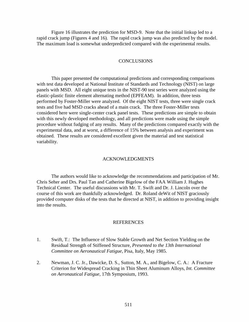
511
Figure 16 illustrates the prediction for MSD-9. Note that the initial linkup led to arapid crack jump (Figures 4 and 16). The rapid crack jump was also predicted by the model.The maximum load is somewhat underpredicted compared with the experimental results.
CONCLUSIONS
This paper presented the computational predictions and corresponding comparisonswith test data developed at National Institute of Standards and Technology (NIST) on largepanels with MSD. All eight unique tests in the NIST-90 test series were analyzed using theelastic-plastic finite element alternating method (EPFEAM). In addition, three testsperformed by Foster-Miller were analyzed. Of the eight NIST tests, three were single cracktests and five had MSD cracks ahead of a main crack. The three Foster-Miller testsconsidered here were single-center crack panel tests. These predictions are simple to obtainwith this newly developed methodology, and all predictions were made using the simpleprocedure without fudging of any results. Many of the predictions compared exactly with theexperimental data, and at worst, a difference of 15% between analysis and experiment wasobtained. These results are considered excellent given the material and test statisticalvariability.
ACKNOWLEDGMENTS
The authors would like to acknowledge the recommendations and participation of Mr.Chris Seher and Drs. Paul Tan and Catherine Bigelow of the FAA William J. HughesTechnical Center. The useful discussions with Mr. T. Swift and Dr. J. Lincoln over thecourse of this work are thankfully acknowledged. Dr. Roland deWit of NIST graciouslyprovided computer disks of the tests that he directed at NIST, in addition to providing insightinto the results.
REFERENCES
1. Swift, T.: The Influence of Slow Stable Growth and Net Section Yielding on theResidual Strength of Stiffened Structure, Presented to the 13th InternationalCommittee on Aeronautical Fatigue, Pisa, Italy, May 1985.
2. Newman, J. C. Jr., Dawicke, D. S., Sutton, M. A., and Bigelow, C. A.: A Fracture
Criterion for Widespread Cracking in Thin Sheet Aluminum Alloys, Int. Committeeon Aeronautical Fatigue, 17th Symposium, 1993.
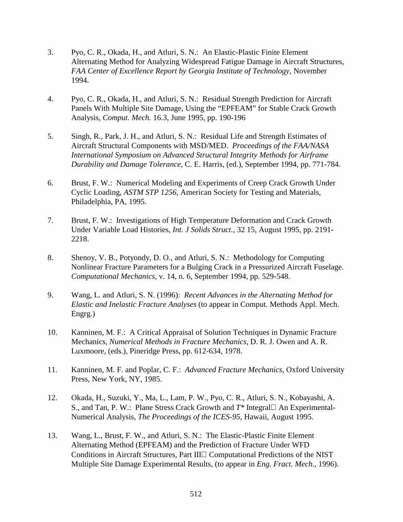
512
3. Pyo, C. R., Okada, H., and Atluri, S. N.: An Elastic-Plastic Finite ElementAlternating Method for Analyzing Widespread Fatigue Damage in Aircraft Structures,FAA Center of Excellence Report by Georgia Institute of Technology, November1994.
4. Pyo, C. R., Okada, H., and Atluri, S. N.: Residual Strength Prediction for Aircraft
Panels With Multiple Site Damage, Using the “EPFEAM” for Stable Crack GrowthAnalysis, Comput. Mech. 16.3, June 1995, pp. 190-196
5. Singh, R., Park, J. H., and Atluri, S. N.: Residual Life and Strength Estimates of
Aircraft Structural Components with MSD/MED. Proceedings of the FAA/NASAInternational Symposium on Advanced Structural Integrity Methods for AirframeDurability and Damage Tolerance, C. E. Harris, (ed.), September 1994, pp. 771-784.
6. Brust, F. W.: Numerical Modeling and Experiments of Creep Crack Growth Under
Cyclic Loading, ASTM STP 1256, American Society for Testing and Materials,Philadelphia, PA, 1995.
7. Brust, F. W.: Investigations of High Temperature Deformation and Crack Growth
Under Variable Load Histories, Int. J Solids Struct., 32 15, August 1995, pp. 2191-2218.
8. Shenoy, V. B., Potyondy, D. O., and Atluri, S. N.: Methodology for Computing
Nonlinear Fracture Parameters for a Bulging Crack in a Pressurized Aircraft Fuselage.Computational Mechanics, v. 14, n. 6, September 1994, pp. 529-548.
9. Wang, L. and Atluri, S. N. (1996): Recent Advances in the Alternating Method for
Elastic and Inelastic Fracture Analyses (to appear in Comput. Methods Appl. Mech.Engrg.)
10. Kanninen, M. F.: A Critical Appraisal of Solution Techniques in Dynamic Fracture
Mechanics, Numerical Methods in Fracture Mechanics, D. R. J. Owen and A. R.Luxmoore, (eds.), Pineridge Press, pp. 612-634, 1978.
11. Kanninen, M. F. and Poplar, C. F.: Advanced Fracture Mechanics, Oxford University
Press, New York, NY, 1985. 12. Okada, H., Suzuki, Y., Ma, L., Lam, P. W., Pyo, C. R., Atluri, S. N., Kobayashi, A.
S., and Tan, P. W.: Plane Stress Crack Growth and T* IntegralAn Experimental-Numerical Analysis, The Proceedings of the ICES-95, Hawaii, August 1995.
13. Wang, L., Brust, F. W., and Atluri, S. N.: The Elastic-Plastic Finite Element
Alternating Method (EPFEAM) and the Prediction of Fracture Under WFDConditions in Aircraft Structures, Part IIIComputational Predictions of the NISTMultiple Site Damage Experimental Results, (to appear in Eng. Fract. Mech., 1996).
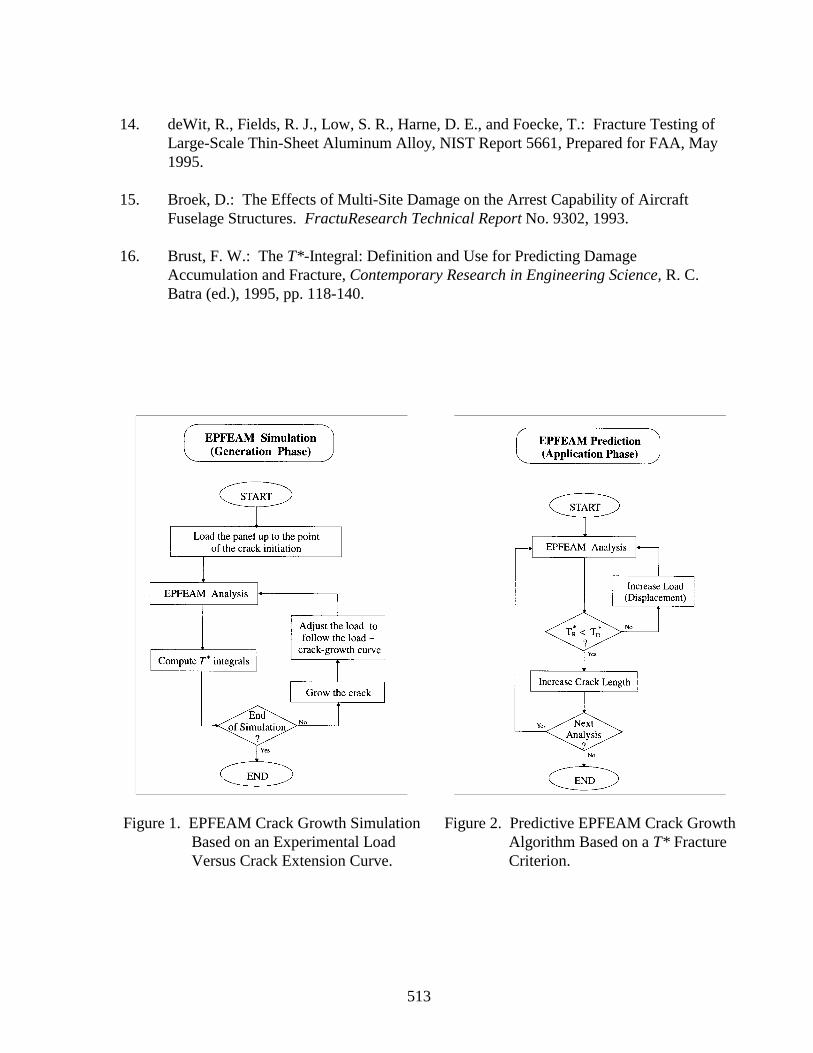
513
14. deWit, R., Fields, R. J., Low, S. R., Harne, D. E., and Foecke, T.: Fracture Testing of
Large-Scale Thin-Sheet Aluminum Alloy, NIST Report 5661, Prepared for FAA, May1995.
15. Broek, D.: The Effects of Multi-Site Damage on the Arrest Capability of Aircraft
Fuselage Structures. FractuResearch Technical Report No. 9302, 1993. 16. Brust, F. W.: The T*-Integral: Definition and Use for Predicting Damage
Accumulation and Fracture, Contemporary Research in Engineering Science, R. C.Batra (ed.), 1995, pp. 118-140.
Figure 1. EPFEAM Crack Growth SimulationBased on an Experimental LoadVersus Crack Extension Curve.
Figure 2. Predictive EPFEAM Crack GrowthAlgorithm Based on a T* FractureCriterion.
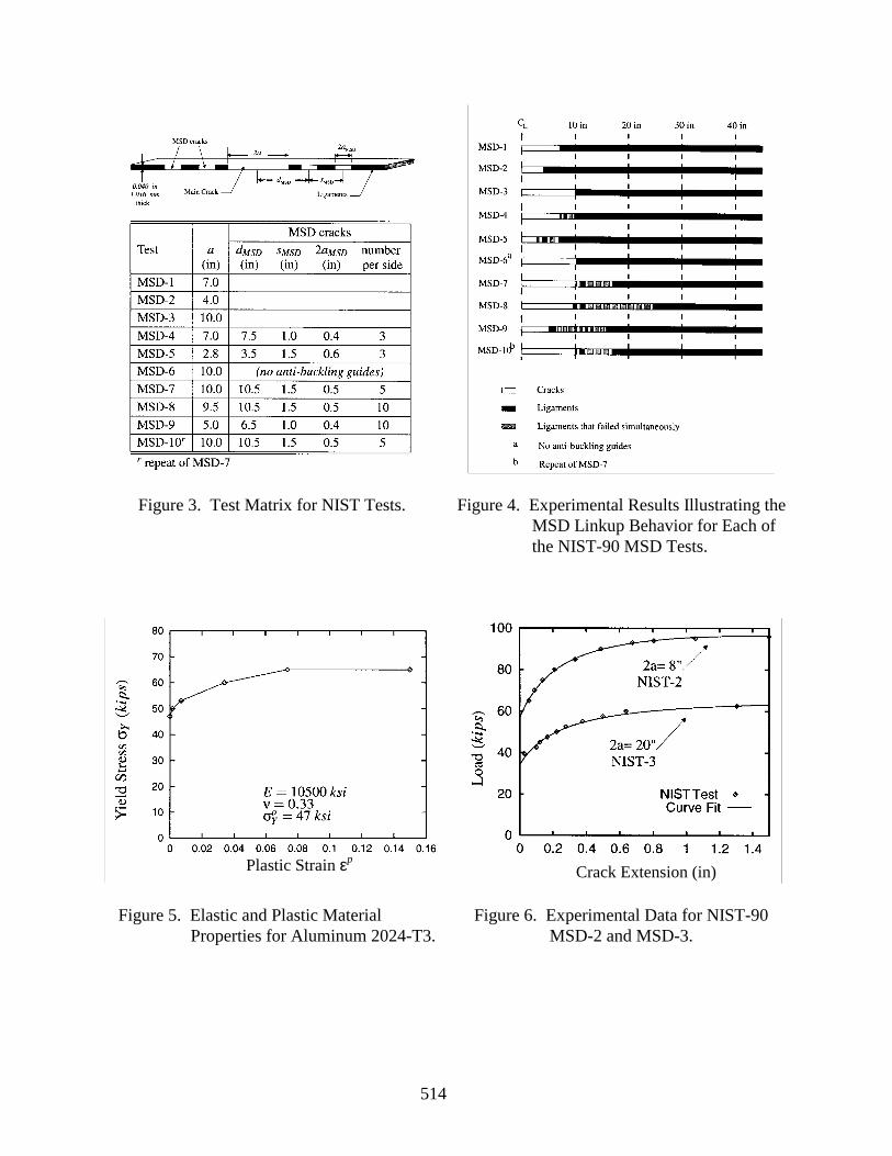
514
Figure 3. Test Matrix for NIST Tests. Figure 4. Experimental Results Illustrating theMSD Linkup Behavior for Each ofthe NIST-90 MSD Tests.
Figure 5. Elastic and Plastic MaterialProperties for Aluminum 2024-T3.
Figure 6. Experimental Data for NIST-90MSD-2 and MSD-3.
Crack Extension (in)Plastic Strain εp
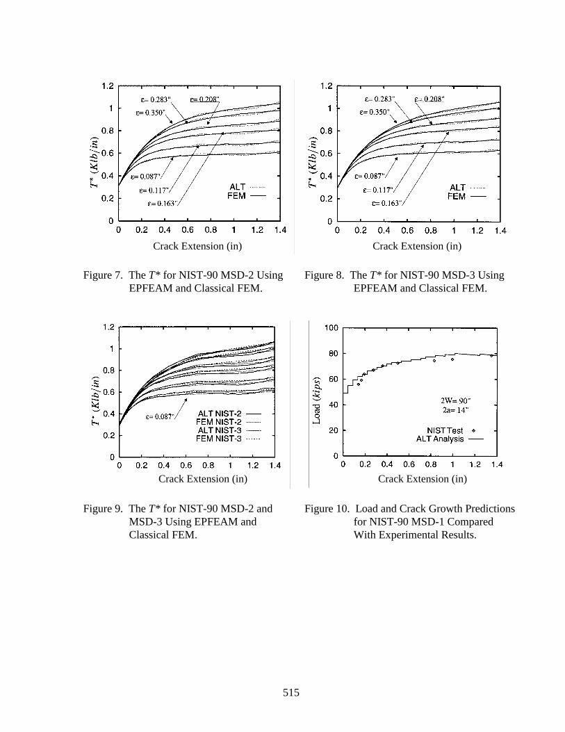
515
Figure 7. The T* for NIST-90 MSD-2 UsingEPFEAM and Classical FEM.
Figure 8. The T* for NIST-90 MSD-3 UsingEPFEAM and Classical FEM.
Figure 9. The T* for NIST-90 MSD-2 andMSD-3 Using EPFEAM andClassical FEM.
Figure 10. Load and Crack Growth Predictionsfor NIST-90 MSD-1 ComparedWith Experimental Results.
Crack Extension (in)Crack Extension (in)
Crack Extension (in)Crack Extension (in)
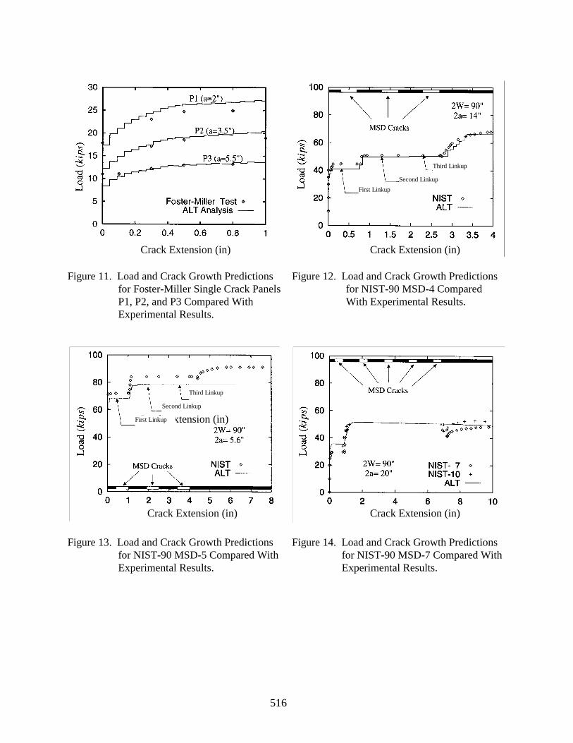
516
First Linkup
Second Linkup
Third Linkup
Figure 11. Load and Crack Growth Predictionsfor Foster-Miller Single Crack PanelsP1, P2, and P3 Compared WithExperimental Results.
Figure 12. Load and Crack Growth Predictionsfor NIST-90 MSD-4 ComparedWith Experimental Results.
Figure 13. Load and Crack Growth Predictionsfor NIST-90 MSD-5 Compared WithExperimental Results.
Figure 14. Load and Crack Growth Predictionsfor NIST-90 MSD-7 Compared WithExperimental Results.
Crack Extension (in)First Linkup
Second Linkup
Third Linkup
Crack Extension (in) Crack Extension (in)
Crack Extension (in) Crack Extension (in)
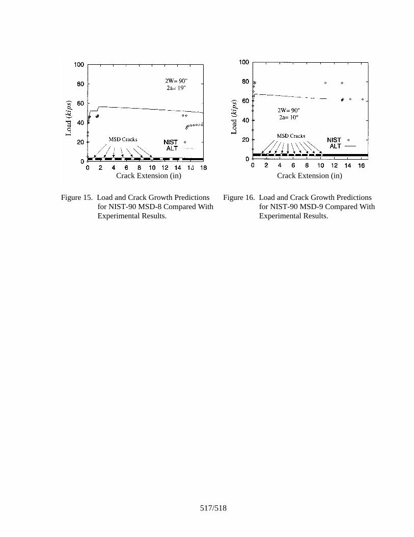
517/518
Figure 15. Load and Crack Growth Predictionsfor NIST-90 MSD-8 Compared WithExperimental Results.
Figure 16. Load and Crack Growth Predictionsfor NIST-90 MSD-9 Compared WithExperimental Results.
Crack Extension (in) Crack Extension (in)
519
PREDICTIONS OF WIDESPREAD FATIGUE DAMAGE THRESHOLD
L. Wang, W. T. Chow, H. Kawai, and S. N. AtluriFAA Center of Excellence for
Computational Modeling of Aircraft StructuresGeorgia Institute of TechnologyAtlanta, Georgia 30332-0356
SUMMARY
Commercial transport aircraft are required to operate under the concept of damagetolerance. This requires that aircraft fuselages and wings tolerate discrete source damagesinduced by foreign objects, such as impact damage due to engine disintegration. Due to thestructural redundancy and the crack arrest capability, the current fleet of commercial aircraftwere initially designed to have sufficient residual strength to sustain discrete source damage.However, fatigue damage during the life of an aircraft can significantly reduce the residualstrength of an aging aircraft. Thus, it is important to predict the severity of the fatiguedamage, since it can reduce the residual strength of an aging aircraft to below the damage-tolerant requirement. It is also important to estimate the remaining fatigue life of an agingaircraft so that inspection, maintenance, and repair can be scheduled before a catastrophicfailure may occur. This paper presents a hierarchical approach for the numerical predictionsof the widespread fatigue damage threshold and the remaining fatigue life of an aging aircraft.In this approach, the global load distribution is obtained using an finite element analysis with acoarse mesh, while the crack(s) is (are) modeled only to a level to determine the load flowredistribution due to its (their) presence. The crack tip parameters are obtained using thefinite element alternating method at the local level. A detailed numerical study is presented toillustrate the typical characteristics of the widespread fatigue damage threshold for an agingaircraft.
INTRODUCTION
The fatigue damage due to the repetitive loading condition of pressurization is one ofthe major concerns among the civil aviation industry. There exists two different types ofapproach in dealing with the multiple-site fatigue damage problem. One of them is theMultiple-Site Damage Threshold (MSDT) approach, the other is the Widespread FatigueDamage Threshold (WFDT) approach [1]. In the MSDT approach the severity of MSD ismeasured by the potential of linkup, while in the WFDT approach, it is indicated by thereduction of residual strength of the aircraft.
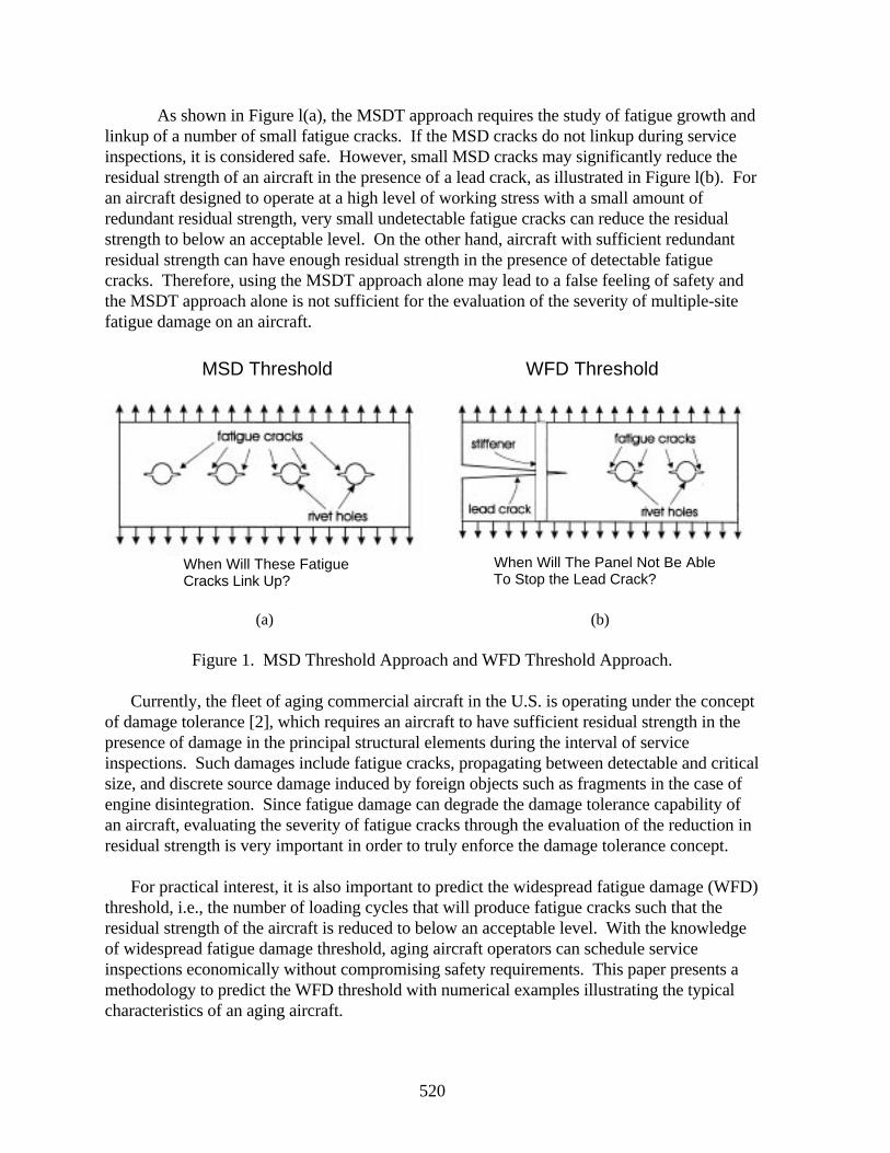
520
As shown in Figure l(a), the MSDT approach requires the study of fatigue growth andlinkup of a number of small fatigue cracks. If the MSD cracks do not linkup during serviceinspections, it is considered safe. However, small MSD cracks may significantly reduce theresidual strength of an aircraft in the presence of a lead crack, as illustrated in Figure l(b). Foran aircraft designed to operate at a high level of working stress with a small amount ofredundant residual strength, very small undetectable fatigue cracks can reduce the residualstrength to below an acceptable level. On the other hand, aircraft with sufficient redundantresidual strength can have enough residual strength in the presence of detectable fatiguecracks. Therefore, using the MSDT approach alone may lead to a false feeling of safety andthe MSDT approach alone is not sufficient for the evaluation of the severity of multiple-sitefatigue damage on an aircraft.
(a) (b)
Figure 1. MSD Threshold Approach and WFD Threshold Approach.
Currently, the fleet of aging commercial aircraft in the U.S. is operating under the conceptof damage tolerance [2], which requires an aircraft to have sufficient residual strength in thepresence of damage in the principal structural elements during the interval of serviceinspections. Such damages include fatigue cracks, propagating between detectable and criticalsize, and discrete source damage induced by foreign objects such as fragments in the case ofengine disintegration. Since fatigue damage can degrade the damage tolerance capability ofan aircraft, evaluating the severity of fatigue cracks through the evaluation of the reduction inresidual strength is very important in order to truly enforce the damage tolerance concept.
For practical interest, it is also important to predict the widespread fatigue damage (WFD)threshold, i.e., the number of loading cycles that will produce fatigue cracks such that theresidual strength of the aircraft is reduced to below an acceptable level. With the knowledgeof widespread fatigue damage threshold, aging aircraft operators can schedule serviceinspections economically without compromising safety requirements. This paper presents amethodology to predict the WFD threshold with numerical examples illustrating the typicalcharacteristics of an aging aircraft.
When Will These FatigueCracks Link Up?
When Will The Panel Not Be AbleTo Stop the Lead Crack?
MSD Threshold WFD Threshold
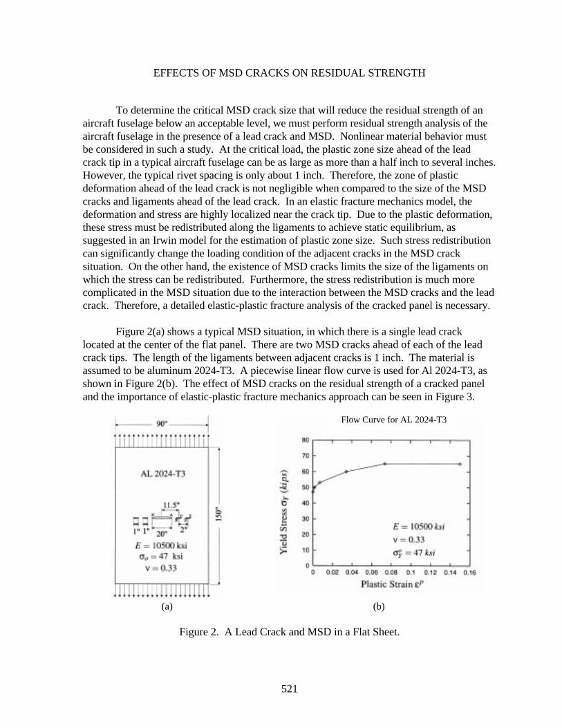
521
EFFECTS OF MSD CRACKS ON RESIDUAL STRENGTH
To determine the critical MSD crack size that will reduce the residual strength of anaircraft fuselage below an acceptable level, we must perform residual strength analysis of theaircraft fuselage in the presence of a lead crack and MSD. Nonlinear material behavior mustbe considered in such a study. At the critical load, the plastic zone size ahead of the leadcrack tip in a typical aircraft fuselage can be as large as more than a half inch to several inches.However, the typical rivet spacing is only about 1 inch. Therefore, the zone of plasticdeformation ahead of the lead crack is not negligible when compared to the size of the MSDcracks and ligaments ahead of the lead crack. In an elastic fracture mechanics model, thedeformation and stress are highly localized near the crack tip. Due to the plastic deformation,these stress must be redistributed along the ligaments to achieve static equilibrium, assuggested in an Irwin model for the estimation of plastic zone size. Such stress redistributioncan significantly change the loading condition of the adjacent cracks in the MSD cracksituation. On the other hand, the existence of MSD cracks limits the size of the ligaments onwhich the stress can be redistributed. Furthermore, the stress redistribution is much morecomplicated in the MSD situation due to the interaction between the MSD cracks and the leadcrack. Therefore, a detailed elastic-plastic fracture analysis of the cracked panel is necessary.
Figure 2(a) shows a typical MSD situation, in which there is a single lead cracklocated at the center of the flat panel. There are two MSD cracks ahead of each of the leadcrack tips. The length of the ligaments between adjacent cracks is 1 inch. The material isassumed to be aluminum 2024-T3. A piecewise linear flow curve is used for Al 2024-T3, asshown in Figure 2(b). The effect of MSD cracks on the residual strength of a cracked paneland the importance of elastic-plastic fracture mechanics approach can be seen in Figure 3.
(a) (b)
Figure 2. A Lead Crack and MSD in a Flat Sheet.
Flow Curve for AL 2024-T3
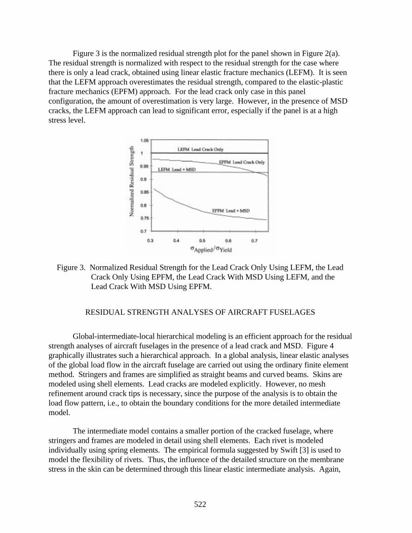
522
Figure 3 is the normalized residual strength plot for the panel shown in Figure 2(a).The residual strength is normalized with respect to the residual strength for the case wherethere is only a lead crack, obtained using linear elastic fracture mechanics (LEFM). It is seenthat the LEFM approach overestimates the residual strength, compared to the elastic-plasticfracture mechanics (EPFM) approach. For the lead crack only case in this panelconfiguration, the amount of overestimation is very large. However, in the presence of MSDcracks, the LEFM approach can lead to significant error, especially if the panel is at a highstress level.
Figure 3. Normalized Residual Strength for the Lead Crack Only Using LEFM, the LeadCrack Only Using EPFM, the Lead Crack With MSD Using LEFM, and theLead Crack With MSD Using EPFM.
RESIDUAL STRENGTH ANALYSES OF AIRCRAFT FUSELAGES
Global-intermediate-local hierarchical modeling is an efficient approach for the residualstrength analyses of aircraft fuselages in the presence of a lead crack and MSD. Figure 4graphically illustrates such a hierarchical approach. In a global analysis, linear elastic analysesof the global load flow in the aircraft fuselage are carried out using the ordinary finite elementmethod. Stringers and frames are simplified as straight beams and curved beams. Skins aremodeled using shell elements. Lead cracks are modeled explicitly. However, no meshrefinement around crack tips is necessary, since the purpose of the analysis is to obtain theload flow pattern, i.e., to obtain the boundary conditions for the more detailed intermediatemodel.
The intermediate model contains a smaller portion of the cracked fuselage, wherestringers and frames are modeled in detail using shell elements. Each rivet is modeledindividually using spring elements. The empirical formula suggested by Swift [3] is used tomodel the flexibility of rivets. Thus, the influence of the detailed structure on the membranestress in the skin can be determined through this linear elastic intermediate analysis. Again,
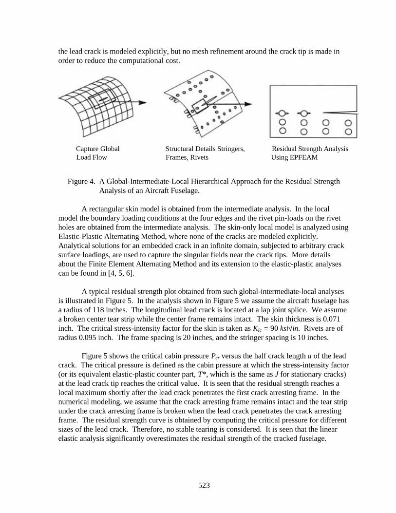
523
the lead crack is modeled explicitly, but no mesh refinement around the crack tip is made inorder to reduce the computational cost.
Figure 4. A Global-Intermediate-Local Hierarchical Approach for the Residual StrengthAnalysis of an Aircraft Fuselage.
A rectangular skin model is obtained from the intermediate analysis. In the localmodel the boundary loading conditions at the four edges and the rivet pin-loads on the rivetholes are obtained from the intermediate analysis. The skin-only local model is analyzed usingElastic-Plastic Alternating Method, where none of the cracks are modeled explicitly.Analytical solutions for an embedded crack in an infinite domain, subjected to arbitrary cracksurface loadings, are used to capture the singular fields near the crack tips. More detailsabout the Finite Element Alternating Method and its extension to the elastic-plastic analysescan be found in [4, 5, 6].
A typical residual strength plot obtained from such global-intermediate-local analysesis illustrated in Figure 5. In the analysis shown in Figure 5 we assume the aircraft fuselage hasa radius of 118 inches. The longitudinal lead crack is located at a lap joint splice. We assumea broken center tear strip while the center frame remains intact. The skin thickness is 0.071inch. The critical stress-intensity factor for the skin is taken as KIc = 90 ksi√in. Rivets are ofradius 0.095 inch. The frame spacing is 20 inches, and the stringer spacing is 10 inches.
Figure 5 shows the critical cabin pressure Pcr versus the half crack length a of the leadcrack. The critical pressure is defined as the cabin pressure at which the stress-intensity factor(or its equivalent elastic-plastic counter part, T*, which is the same as J for stationary cracks)at the lead crack tip reaches the critical value. It is seen that the residual strength reaches alocal maximum shortly after the lead crack penetrates the first crack arresting frame. In thenumerical modeling, we assume that the crack arresting frame remains intact and the tear stripunder the crack arresting frame is broken when the lead crack penetrates the crack arrestingframe. The residual strength curve is obtained by computing the critical pressure for differentsizes of the lead crack. Therefore, no stable tearing is considered. It is seen that the linearelastic analysis significantly overestimates the residual strength of the cracked fuselage.
Capture Global Load Flow
Structural Details Stringers, Frames, Rivets
Residual Strength Analysis Using EPFEAM
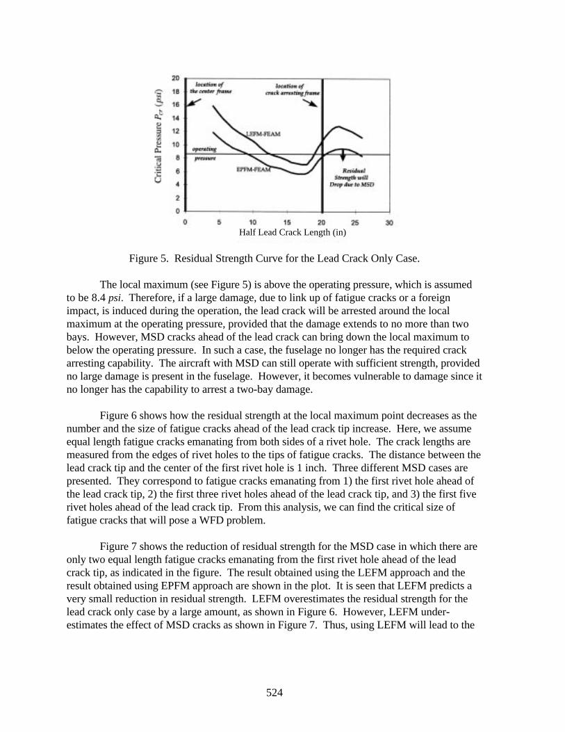
524
Figure 5. Residual Strength Curve for the Lead Crack Only Case.
The local maximum (see Figure 5) is above the operating pressure, which is assumedto be 8.4 psi. Therefore, if a large damage, due to link up of fatigue cracks or a foreignimpact, is induced during the operation, the lead crack will be arrested around the localmaximum at the operating pressure, provided that the damage extends to no more than twobays. However, MSD cracks ahead of the lead crack can bring down the local maximum tobelow the operating pressure. In such a case, the fuselage no longer has the required crackarresting capability. The aircraft with MSD can still operate with sufficient strength, providedno large damage is present in the fuselage. However, it becomes vulnerable to damage since itno longer has the capability to arrest a two-bay damage.
Figure 6 shows how the residual strength at the local maximum point decreases as thenumber and the size of fatigue cracks ahead of the lead crack tip increase. Here, we assumeequal length fatigue cracks emanating from both sides of a rivet hole. The crack lengths aremeasured from the edges of rivet holes to the tips of fatigue cracks. The distance between thelead crack tip and the center of the first rivet hole is 1 inch. Three different MSD cases arepresented. They correspond to fatigue cracks emanating from 1) the first rivet hole ahead ofthe lead crack tip, 2) the first three rivet holes ahead of the lead crack tip, and 3) the first fiverivet holes ahead of the lead crack tip. From this analysis, we can find the critical size offatigue cracks that will pose a WFD problem.
Figure 7 shows the reduction of residual strength for the MSD case in which there areonly two equal length fatigue cracks emanating from the first rivet hole ahead of the leadcrack tip, as indicated in the figure. The result obtained using the LEFM approach and theresult obtained using EPFM approach are shown in the plot. It is seen that LEFM predicts avery small reduction in residual strength. LEFM overestimates the residual strength for thelead crack only case by a large amount, as shown in Figure 6. However, LEFM under-estimates the effect of MSD cracks as shown in Figure 7. Thus, using LEFM will lead to the
Half Lead Crack Length (in)
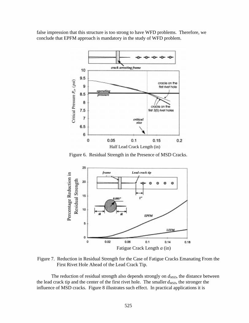
525
false impression that this structure is too strong to have WFD problems. Therefore, weconclude that EPFM approach is mandatory in the study of WFD problem.
Figure 6. Residual Strength in the Presence of MSD Cracks.
Figure 7. Reduction in Residual Strength for the Case of Fatigue Cracks Emanating From theFirst Rivet Hole Ahead of the Lead Crack Tip.
The reduction of residual strength also depends strongly on dMSD, the distance betweenthe lead crack tip and the center of the first rivet hole. The smaller dMSD, the stronger theinfluence of MSD cracks. Figure 8 illustrates such effect. In practical applications it is
Lead crack tipframe
Half Lead Crack Length (in)
Fatigue Crack Length a (in)
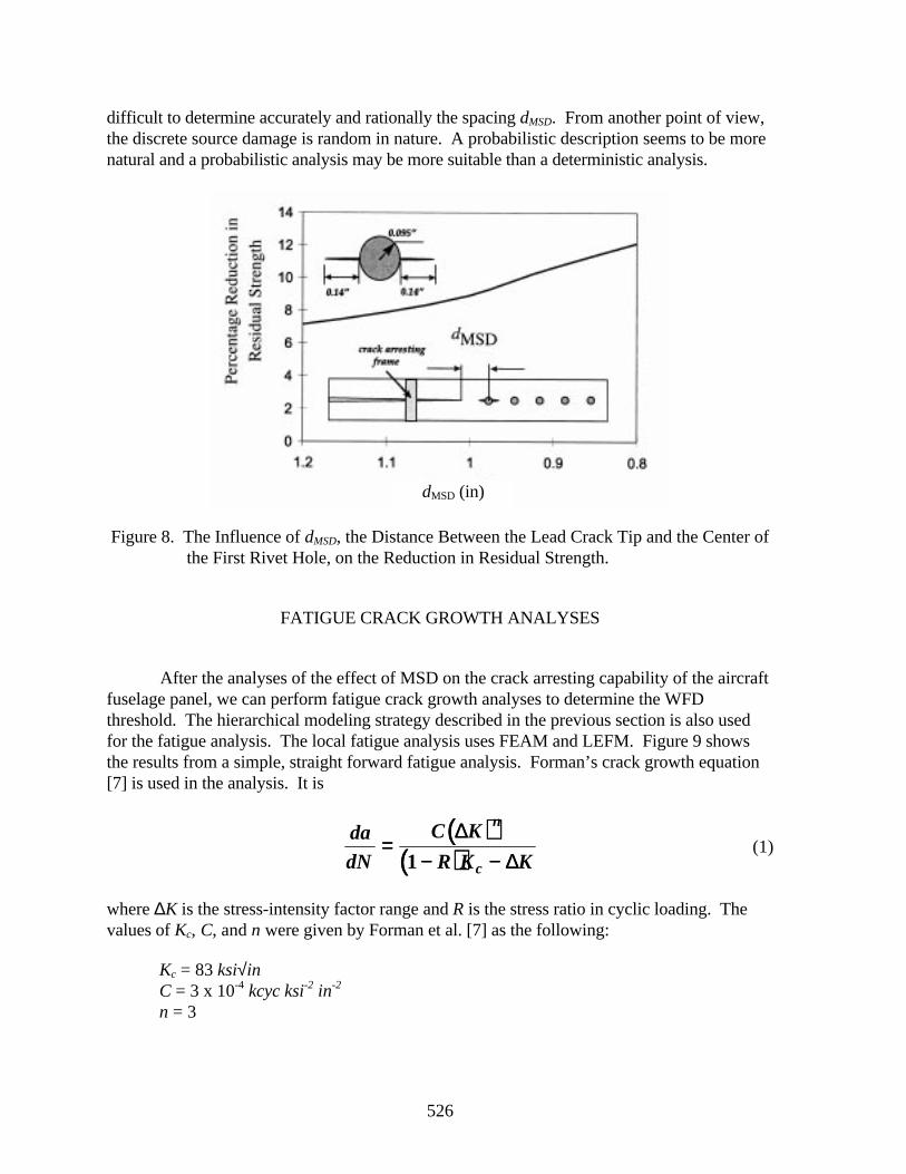
526
difficult to determine accurately and rationally the spacing dMSD. From another point of view,the discrete source damage is random in nature. A probabilistic description seems to be morenatural and a probabilistic analysis may be more suitable than a deterministic analysis.
Figure 8. The Influence of dMSD, the Distance Between the Lead Crack Tip and the Center ofthe First Rivet Hole, on the Reduction in Residual Strength.
FATIGUE CRACK GROWTH ANALYSES
After the analyses of the effect of MSD on the crack arresting capability of the aircraftfuselage panel, we can perform fatigue crack growth analyses to determine the WFDthreshold. The hierarchical modeling strategy described in the previous section is also usedfor the fatigue analysis. The local fatigue analysis uses FEAM and LEFM. Figure 9 showsthe results from a simple, straight forward fatigue analysis. Forman’s crack growth equation[7] is used in the analysis. It is
(( ))(( ))
dadN
C K
R K K
n
c==
−− −−∆∆
∆∆1(1)
where ∆K is the stress-intensity factor range and R is the stress ratio in cyclic loading. Thevalues of Kc, C, and n were given by Forman et al. [7] as the following:
Kc = 83 ksi√inC = 3 x 10⁻⁴ kcyc ksi-2 in-2
n = 3
dMSD (in)
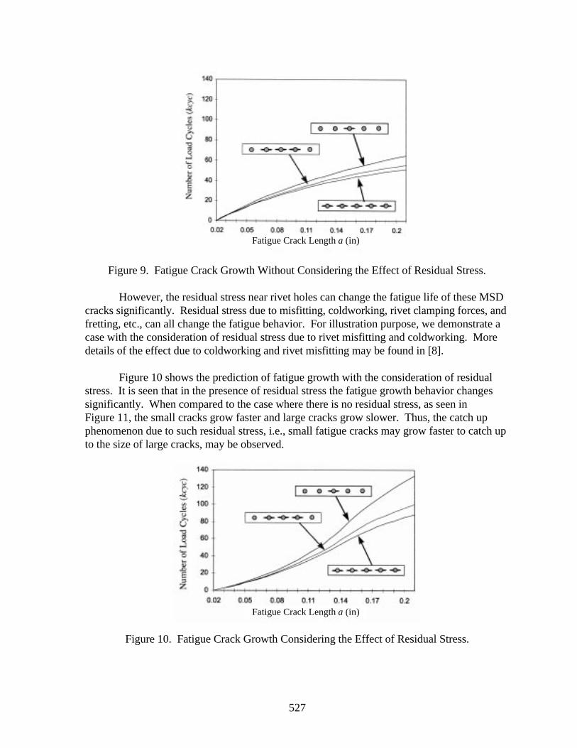
527
Figure 9. Fatigue Crack Growth Without Considering the Effect of Residual Stress.
However, the residual stress near rivet holes can change the fatigue life of these MSDcracks significantly. Residual stress due to misfitting, coldworking, rivet clamping forces, andfretting, etc., can all change the fatigue behavior. For illustration purpose, we demonstrate acase with the consideration of residual stress due to rivet misfitting and coldworking. Moredetails of the effect due to coldworking and rivet misfitting may be found in [8].
Figure 10 shows the prediction of fatigue growth with the consideration of residualstress. It is seen that in the presence of residual stress the fatigue growth behavior changessignificantly. When compared to the case where there is no residual stress, as seen inFigure 11, the small cracks grow faster and large cracks grow slower. Thus, the catch upphenomenon due to such residual stress, i.e., small fatigue cracks may grow faster to catch upto the size of large cracks, may be observed.
Figure 10. Fatigue Crack Growth Considering the Effect of Residual Stress.
Fatigue Crack Length a (in)
Fatigue Crack Length a (in)
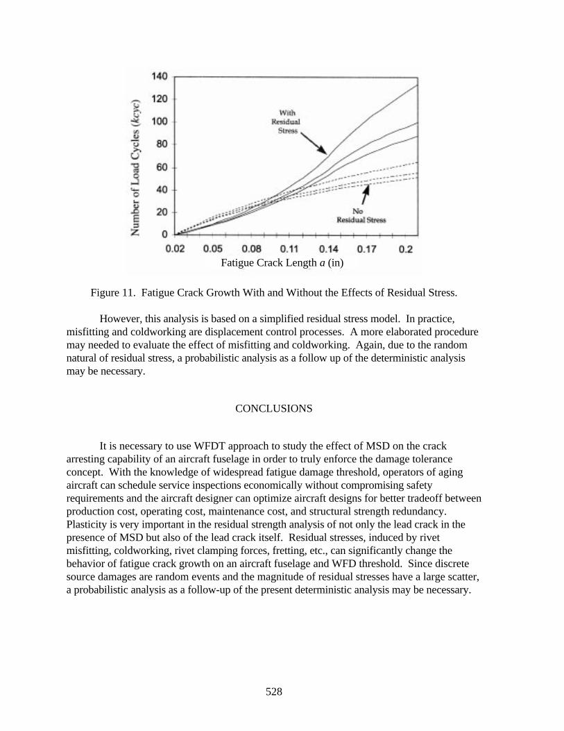
528
Figure 11. Fatigue Crack Growth With and Without the Effects of Residual Stress.
However, this analysis is based on a simplified residual stress model. In practice,misfitting and coldworking are displacement control processes. A more elaborated proceduremay needed to evaluate the effect of misfitting and coldworking. Again, due to the randomnatural of residual stress, a probabilistic analysis as a follow up of the deterministic analysismay be necessary.
CONCLUSIONS
It is necessary to use WFDT approach to study the effect of MSD on the crackarresting capability of an aircraft fuselage in order to truly enforce the damage toleranceconcept. With the knowledge of widespread fatigue damage threshold, operators of agingaircraft can schedule service inspections economically without compromising safetyrequirements and the aircraft designer can optimize aircraft designs for better tradeoff betweenproduction cost, operating cost, maintenance cost, and structural strength redundancy.Plasticity is very important in the residual strength analysis of not only the lead crack in thepresence of MSD but also of the lead crack itself. Residual stresses, induced by rivetmisfitting, coldworking, rivet clamping forces, fretting, etc., can significantly change thebehavior of fatigue crack growth on an aircraft fuselage and WFD threshold. Since discretesource damages are random events and the magnitude of residual stresses have a large scatter,a probabilistic analysis as a follow-up of the present deterministic analysis may be necessary.
Fatigue Crack Length a (in)
529/530
ACKNOWLEDGMENTS
The authors would like to acknowledge the support from the FAA William J. HughesTechnical Center to the Center of Excellence for Computational Modeling of AircraftStructures, Georgia Institute of Technology.
REFERENCES
1. Jeong, D. Y. and Tong, P.: Threshold of Multiple Site Damage in Aging Airplanes.Structural Integrity in Aging Aircraft, ASME-AD V.47, 1995, pp. 63-71.
2. Swift, T.: Damage Tolerance Assessment of Commercial Airframes. Fracture
Problems in the Transportation Industry ASCE, 1985, pp. 97-138. 3. Swift, T.: Fracture Analysis of Stiffened Structure. Damage Tolerance of Metallic
Structures, ASTM STP 842, 1984, pp. 69-107. 4. Nikishkov, G. P. and Atluri, S. N.: Analytical-Numerical Alternating Method for
Elastic-Plastic Analysis of Cracks. Computational Mechanics, v.13, no. 6, 1994.pp. 427-442.
5. Wang, L. H. and Atluri, S. N.: Implementation of the Schwartz-Neumann Alternating
Method for Collinear Multiple Cracks with Mixed Type of Boundary Conditions.Computational Mechanics, v. 16, no. 4, 1995, pp. 266-271.
6. Wang, L. and Atluri, S. N. (1996): Recent Advances in the Alternating Method for
Elastic and Inelastic Fracture Analyses (to appear in Comput. Methods Appl. Mech.Engrg.).
7. Forman, R. G., Kearney, V. E., and Engle, R. M.: Numerical Analysis of Crack
Propagation in Cyclic-Loaded Structures, J. Basic Engg. 89, 1967, pp. 459-464. 8. Park, J. H. and Atluri, S. N.: Fatigue Growth of Multiple-Cracks Near a Row of
Fastener Holes in a Fuselage Lap Joint, Computational Mechanics, v. 13 no. 3, 1993.pp. 189-203.
531
PROBABILITY AND STATISTICS MODELING OFCONSTITUENT PARTICLES AND CORROSION PITS AS A
BASIS FOR MULTI PLE-SITE DAMAGE ANALYSIS 1
N. R. Cawley, D. G. Harlow, and R. P. WeiDepartment of Mechanical Engineering and Mechanics
Lehigh University19 Memorial Drive West
Bethlehem, PA 18015-3085
SUMMARY
A probability model for the growth of corrosion pits in aluminum alloys in aqueousenvironments, in which the focus is the role of clustered particles, is suggested as a basis forestimating the distributions in size and location of fatigue cracks, as a function of time, foruse in multiple-site damage (MSD) analyses. MSD is a condition in which multiple fatiguecracks occur within the same structural element, which is precipitated by pitting corrosion.The model replaces the practice of assuming the distributions for the size and location ofMSD. Statistical distributions, estimated from experimental observations of 2024-T3aluminum alloy, for the random size, density, and location of constituent particles are used asinput for a mechanistically based probability model for severe corrosion pit growth. Pittinginitiates at constituent particles, which are either anodic or cathodic relative to the matrix, andinvolves complex electrochemical processes. Local interactions between particles and thematrix enhance the growth rate. Spatial statistics models for cluster processes have beenmodified to characterize constituent particles, which are clustered randomly in size andshape.
INTRODUCTION
Multiple-site damage is a condition in which fatigue damage or cracks are at morethan one site within the same structural element. MSD is of serious concern in terms of theintegrity and safety of aging systems. In aging airplanes, for example, MSD may occur as aresult of fatigue cracking at rivet holes along fuselage lap joints. Currently, statisticaldistributions for the size and location of MSD in aging airplanes are assumed. Thisprocedure is unsatisfactory because of the absence of a rational basis for their selection andfor estimating the time evolution of damage. A mechanistically based model for estimatingthe time evolution of these distributions of MSD, therefore, is needed and is discussed herein.
1 This research was supported in part by the Air Force Office of Scientific Research under Grant F49620-93-1-0426 and by the Federal Aviation Administration under Grant 92-G-0006.
532
Pitting corrosion in aluminum alloys is recognized as an important precursor for theonset of fatigue crack growth, and it is influenced by the nature and distribution of theconstituent particles in the alloys. Probability and statistical modeling of constituent particlesand corrosion pits, coupled with fatigue growth analysis, therefore, provide a rational basisfor MSD analyses. The primary thrust herein is to describe some the key features necessaryfor the development of a mechanistically based probability model for the growth of corrosionpits. The success of this approach is highly dependent on the accuracy of the mechanisticmodel for the corrosion process and on the proper identification of the random variables (rvs)that affect the process. The goal of this effort is to estimate the random pit size at an arbitrarytime and location. Since fatigue cracks emanate from severe corrosion pits, the probabilitydistribution for pit size at a specified location is a precursor to MSD analysis. A plausiblemechanistic model is considered for the evolution of pitting corrosion and its probabilisticcharacter. The model focuses on the growth of corrosion pits in an aluminum alloy in anaqueous environment. The main sources of variability in the model are from the mechanicaland corrosion properties of the alloy and the electrochemical behavior induced by theenvironment. The significance of the variables is evaluated by using parameter values andassumed probability distributions which are typical in experimental observations.
DEVELOPMENT OF THE MODEL
The crucial aspect in mechanistically based probability modeling is the description ofthe damage process. The damage of interest is the growth of corrosion pits. The model ismotivated by environmental effects on bare surfaces, e.g., the interior surface of rivet holes.Damage nucleates on bare surfaces as pits formed by localized galvanic corrosion nearexposed constituent particles. As pits grow, neighboring particles are exposed and furthercontribute to growth. The process continues until a critical pit size is reached from which asmall corrosion fatigue crack nucleates with high probability. Randomness in materialproperties and their sensitivity to the environment are represented explicitly. Because adetailed mechanistic model for pit growth is not developed fully, well-established empiricaltraits are incorporated. The corrosion pit size, as a function of the exposure time to theenvironment, is the key variable in this effort. The goal is to find the time dependentcumulative distribution function (cdf) for pit size. It is the cdf which accounts for scatter andwhich allows for identification, estimation, and prediction of reliability.
Constituent particles behave cathodically or anodically relative to the matrix.Corrosion pits formed by the dissolution of anodic particles terminate their growth, or are atleast severely retarded, when the anodic particle is nearly dissolved [1]. Cathodic particles,however, promote dissolution of the adjacent matrix. Thus, cathodic particles are assumed tobe critical for pit growth. The particles for 12 different square fields, 800 µm × 800 µm, wereanalyzed, principally by size and shape, to distinguish the cathodic particles.
Modeling the spatial statistics of particles is not easy [2, 3]; however, some of theproperties can be obtained readily. Figure 1 shows a polished section of the rolling surface of
533
2024-T3 alloy before exposure to any environment. Cross sections of constituent particles,which have random size and shape, are manifest. Notice the particle clustering, where thepredominant cluster pattern appears to be somewhat aligned, principally in the rollingdirection. Clearly, a cluster may have a long dimension of several hundred µm. Particleclustering and alignment are attributed to processing. Geometrical properties of the particlesand clusters, observed on polished sections, are measured from SEM micrographs. Thus,modeling the spatial statistics for particle clustering in the alloy is needed for predictions ofthe growth of corrosion.
Severe pitting is caused by interaction between the matrix and a cluster or clusters ofsubsurface particles, which form local galvanic cells to sustain dissolution. Figure 2 showsSEM micrographs of the cross section of pits formed from clusters of constituent particles. Theinset shows the pits from the specimen surface. The larger pit is approximately 500 µm long,70 µm wide at the surface, and 300 µm deep at this section. The overall shape reflects theplanar distribution of constituent particles, which happen to be cathodic. An SEMmicrofractograph of a fatigue crack origin is shown in Figure 3. The crack originates at a pitdisplayed by the dark region at the center of the microfractograph. The features of the origin areidentical to those of the deeper pit in Figure 2. The associated surface features of the fatigueorigin, which are not shown, are also identical to those shown in the inset in Figure 2. Thesecomparisons clearly link severe localized pitting to corrosion fatigue crack nucleation. Sinceparticle clustering is critical, it must be modeled appropriately. Major damaged regions in thealloy can range from 50 to 150 µm in width and from 100 to 2,000 µm in length relative tothe primary rolling direction [4]. The density of severe pits is approximately one pit/mm2 [4].
The cluster size was estimated by the nearest neighbor cdf, which describes theminimum distance between each particle and its nearest neighbor, computed betweencentroids. The distances are fit quite well by a Weibull cdf, and the parameters, found bymaximum likelihood, are as follows: shape parameter, .α = 180 and scale parameter, .β µ= 42 34 m . The scatter is 57%, and the mean is .µ µ= 37 65 m . The assumed clusteringcriterion is that two particles are clustered if their distance is less than the mean µ . Figure 4is a spatial plot of the centroids of the cathodic particles on a polished section of the rollingsurface of 2024-T3 alloy. The clusters are shown explicitly. A complete description of thecluster analysis is in [3]. Let Nc be the rv for the number of cathodic particles in a cluster.
The estimated cdf for Nc is
Pr . ;.p N k k kk c= = = ≥−0 725 12 41 . (1)
The dilemma is that large clusters lead to the most severe damage, but yet, they are rare. Forexample, in the 7.68 mm2 observed, only 8 clusters containing more than 9 particles werefound of which three had 11, one had 12, one had 15, and one had 22 particles. For animproved estimate additional data are required.
534
Following [5, 6], it is assumed that pits grow at a constant volumetric rate dV/dt givenby
( ) ( )[ ]dV dt MI nF H RTPo= −ρ exp ∆ (2)
where M is the molecular weight of the material, n is the valence, F = 96514 c/mol isFaraday’s constant, ρ is the density, ∆H is the activation energy, R = 8.314 J/mol-K is theuniversal gas constant, T is the absolute temperature, and IPo is the pitting current
coefficient. A mature corrosion pit is geometrically quite complex (Figure 2). As a firstapproximation, the shape is assumed to be half of a prolate spheroid. The orientation of a pitdepends on the location on the aircraft. For example, the high-stress region of a rivet holelocated on the fuselage is an S-T surface of the alloy. A severe pit emanating from such alocation is modeled by a prolate spheroid in which the major axis represents the depth of thepit. The volume is
( )V ab= 2 3 2ππ (3)
where a and b are half the lengths of the major and minor axes, respectively. Alternatively,the high-stress region of a rivet hole located on a wing is the S-L surface of the alloy. Asevere pit originating from this location should be approximated by a prolate spheroid inwhich the minor axis represents the depth. The volume of such a shape is similar to (3)except that the roles of the axes are reversed, i.e., a and b are one-half the lengths of theminor and major axes, respectively. Clearly, the location of a severe pit is essential forproper modeling. Herein, the analysis will be restricted to an application representative of thefuselage.
The time dependent behavior of the axes a and b in (3) is required for dV/dt. Fromobservations, it is assumed that the aspect ratio φk is constant but dependent on the cathodic
particle cluster size k. Thus,
b a kk k= ≥ ≤φ φ, ,0 1. (4)
When φk = 1, the pit growth is hemispherical, [6]. Since dV/dt is assumed to be constant, but
dependent on the cluster size k, it is clear from (2) that the pitting current constant IPolikewise depends on k. Let ao be the initial pit radius, then meshing all of the appropriate
equations yields the following:
( ) ( ) ( ) ( )[ ]2 3 2 3 3πφ ρk o pa a MI k nF H RT to
− = −( ) exp ∆ , (5)
Further details are available in [7].
535
SELECTION OF DETERMINISTIC AND RANDOM VARIABLES
The behavior of an aluminum alloy exposed to an aqueous environment isemphasized. Table 1 lists the deterministic values used in the computations. Thetemperatures are typical of operating temperatures, and ∆H of 30 kJ/mol is reasonable foraluminum alloys, [8, 9]. Estimation of the aspect ratio φk is problematic. A rough
approximation was obtained by empirically estimating the ratio of the longest and shortestchords of a simple convex shape which circumscribes each cluster. The estimations are fairlygood for clusters with less than six particles; however, for the remaining sizes, the data aretoo limited to be accurate. Since large clusters are most important for damage, the sampleaverage is the only reasonable estimate for φk.
The cluster size Nc, which is directly related to the material composition, is assumed
to be a rv with cdf given in (1). The initial pit size ao, which is associated with the size of the
cross section of the surface particle, and the pitting current coefficient IPo, which reflects the
scatter in the electrochemical pit growth, are assumed to be rvs. Extensive experimentaltesting is needed to characterize each rv, and because the cdfs are unknown, the standardthree parameter Weibull cdf is assumed for ao and IPo, [7]. These approximations are
intended to be typical, but they are not necessarily quantitatively accurate. Table 2 containsthe assumed parameter values for the Weibull cdfs. The cluster size k and ao are assumed to
be independent, but IPo is definitely dependent on k because the electrochemical process
depends on the interaction between the particles and the matrix. The assumed numericalvalues are acceptable for illustration purposes; however, for a specific physical applicationthe identification and estimation of these parameters are very important. This is preciselywhere accurate and statistical modeling is required.
RESULTS AND DISCUSSION
The cdf for the pit size is a function of the underlying rvs given the cluster size k.Since it is assumed that the pit size V and depth a are related by (3) and (4), then thecomputation for the cdf for the pit depth F(d; t) is required. Thus, F(d; t) must be computedas an application of law of total probability, i.e.,
F d t a d N k t N k F d t N kc ck
k ck
( ; ) Pr ; Pr ( ; )Pr ,= ≤ = = = =≥ ≥∑ ∑
1 1
(6)
where Fk(d; t) is the conditional cdf for the pit depth given a cluster size of k and where the
distribution for Nc is given in (1). Given that Nc = k, the marginal cdfs for IPo(k) and ao are
536
used to find Fk(d; t). To avoid excessive numerical difficulty, these conditional cdfs are
estimated by Monte Carlo simulation, [7].
Figure 5 shows the conditional cdfs Fk(x; t) for a time t = 3 days of exposure to the
environment, given the cluster size k = 2, 4, 6, 8, and 10. The cdfs are spread over a broadrange as k increases indicating that the variability increases as the cluster size increases. Thevariability is a reflection of the scatter associated with all of the rvs. The median pit depthsrange from 5.3 to 17.2 µm. The reason for the almost vertical lower tails is that there is aminimum pit depth associated with the assumed model. The minimum depth is quitesensitive to the cluster aspect ratio φk, temperature T, and the time t.
Figure 6 shows the conditional cdfs as a function of time when t = 1, 2, 3, 4, and 5days, given a cluster size of k = 22. This corresponds to the largest experimentally observedcluster defined by the interparticle distance criterion. Since there was only one suchobservation, the statistical confidence is limited severely. Because the cdfs are essentiallyparallel, the variability is approximately the same for each cdf. Notice that the scatter israther large. The median depths range from 11.5 to 19.8 µm.
One crucial aspect of mechanistically based probability modeling is the identificationof the variables. This application highlights the need for good observations because the mostneeded information is the most difficult to obtain. Large clusters are the most probable sitesfor severe damage, but their density is very low, implying limited observations. The need forimproved mechanistic descriptions for the pit growth is equally clear. Greater accuracy inmodeling directly results in greater accuracy in reliability estimations.
An important application of this effort is the estimation of the frequency of MSD. Atypical sheet of 1.6 mm thickness may contain many rivet holes with a diameter of about 5mm. The high-stress region in each rivet hole is about 4 mm2. Therefore, the probability ofeach rivet hole having at least one large cluster in the high-stress area is high. Theprobability density function (pdf) for the pit size, derived from (6), gives the frequency of pitdepths. The pdf is used for estimating the probability of finding a pit of a given size in thehigh-stress area. Figure 7 shows an estimate of the pdf for the pit depth when t = 3 days. Thebimodal behavior is apparent. The scatter is considerable, and the median of about 9 µmoccurs at the peak of the dominant mode. Since the pdf is highly dependent on the precedingassumptions, Figure 7 is only illustrative. Nevertheless, the qualitative character is striking.There is a vast difference in the behavior of pits encompassing small clusters as opposed tothose generated by larger clusters. As the time of exposure to the environment increases, thefrequency of large pits also increases. Thus, the role of pit size and its pdf is a precursor formeaningful MSD assessment.
537
SUMMARY
A probability model has been developed for the growth of corrosion pits foraluminum alloys in aqueous environments. The focus has been the cdf for the size of the pitfor a fixed time. This model assumes that the growth of corrosion pits can be approximatedgeometrically by prolate spheroids. The new feature of the modeling is the inclusion ofparticle interaction within clusters to enhance pit growth.
The probabilistic nature of the pit growth, as a function of the time of exposure to theenvironment, was assessed primarily as a function of particle cluster size. The effect oftemperature was considered. The results are qualitatively consistent, and the trend of thecalculations is in accord with typical observations. Also the need for this analysis in MSDassessment was discussed. This effort illustrates that mechanistic probability modeling isneeded to adequately describe complex pit growth. It is apparent that better mechanisticunderstanding of corrosion pit growth and improved characterization of the key rvs iswarranted.
REFERENCES
1. G. Chen, M. Gao, and R.P. Wei: Microconstituent-Induced Pitting Corrosion inAluminum Alloy 2024-T3. Corrosion 52 (1996) 8-15.
2. D.G. Harlow, N.R. Cawley, and R.P. Wei: Spatial Statistics of Particles and
Corrosion Pits in 2024-T3 Aluminum Alloy. Proc. 15th Canadian Congress ofApplied Mechanics, B. Tabarrok and S. Dost, eds., Fleming Express Press Ltd.,Victoria, B.C., vol 1 (1995) 116-117.
3. N.R. Cawley: Models for the Spatial Statistics of Constituent Particles and Corrosion
Pits. Ph.D. Dissertation, Lehigh University, Bethlehem, PA, 1995. 4. G. Chen, C.-M. Liao, K.-C. Wan, M. Gao, and R.P. Wei: Pitting Corrosion and
Fatigue Crack Nucleation. Effects of the Environment on the Initiation of CrackGrowth, ASTM STP 1298, W.A. Van Der Sluys, R.S. Piascik, and R. Zawierucha,eds., 1997, to appear.
5. Y. Kondo: Prediction of Fatigue Crack Initiation Life Based on Pit Growth.
Corrosion 45 (1989) 7-11. 6. D.G. Harlow and R.P. Wei: Probability Approach for Prediction of Corrosion and
Corrosion Fatigue Life. AIAA J. 32 (1994) 2073-2079. 7. D.G. Harlow and R.P. Wei: Probability Modeling for the Growth of Corrosion Pits.
Structural Integrity in Aging Aircraft, AD-Vol.47, C.I. Chang and C.T. Sun, eds.,ASME, New York, (1995) 185-194.
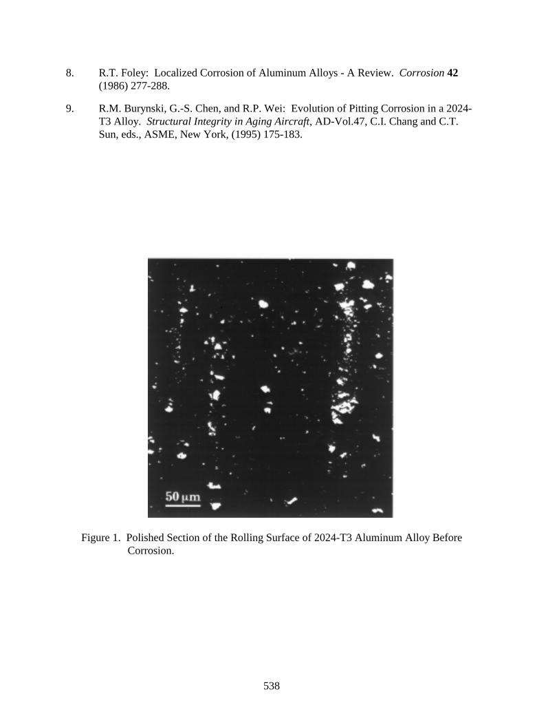
538
8. R.T. Foley: Localized Corrosion of Aluminum Alloys - A Review. Corrosion 42(1986) 277-288.
9. R.M. Burynski, G.-S. Chen, and R.P. Wei: Evolution of Pitting Corrosion in a 2024-
T3 Alloy. Structural Integrity in Aging Aircraft, AD-Vol.47, C.I. Chang and C.T.Sun, eds., ASME, New York, (1995) 175-183.
Figure 1. Polished Section of the Rolling Surface of 2024-T3 Aluminum Alloy BeforeCorrosion.
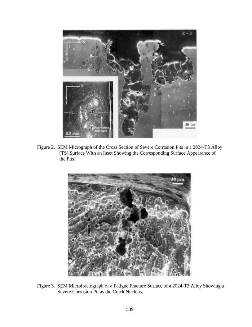
539
Figure 2. SEM Micrograph of the Cross Section of Severe Corrosion Pits in a 2024-T3 Alloy(TS) Surface With an Inset Showing the Corresponding Surface Appearance ofthe Pits.
Figure 3. SEM Microfractograph of a Fatigue Fracture Surface of a 2024-T3 Alloy Showing aSevere Corrosion Pit as the Crack Nucleus.
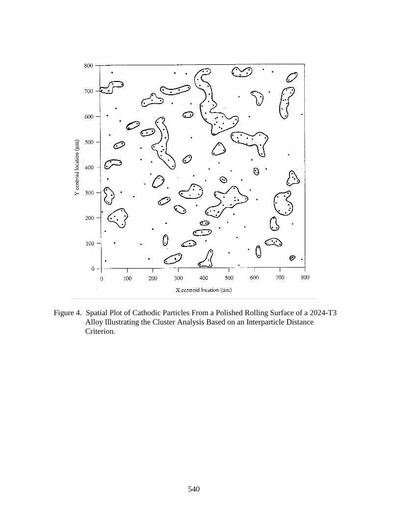
540
Figure 4. Spatial Plot of Cathodic Particles From a Polished Rolling Surface of a 2024-T3Alloy Illustrating the Cluster Analysis Based on an Interparticle DistanceCriterion.
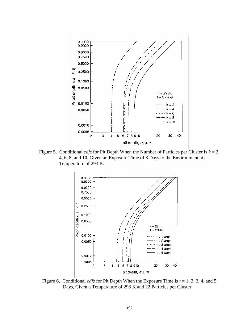
541
Figure 5. Conditional cdfs for Pit Depth When the Number of Particles per Cluster is k = 2,4, 6, 8, and 10, Given an Exposure Time of 3 Days to the Environment at aTemperature of 293 K.
Figure 6. Conditional cdfs for Pit Depth When the Exposure Time is t = 1, 2, 3, 4, and 5Days, Given a Temperature of 293 K and 22 Particles per Cluster.
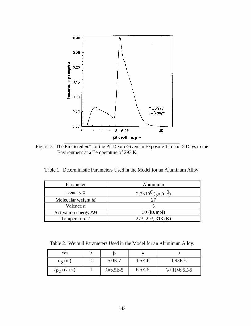
542
Figure 7. The Predicted pdf for the Pit Depth Given an Exposure Time of 3 Days to theEnvironment at a Temperature of 293 K.
Table 1. Deterministic Parameters Used in the Model for an Aluminum Alloy.
Table 2. Weibull Parameters Used in the Model for an Aluminum Alloy.
Parameter Aluminum
Density ρ 2.7×10⁶ (gm/m3)Molecular weight M 27
Valence n 3Activation energy ∆H 30 (kJ/mol)
Temperature T 273, 293, 313 (K)
rvs α β γ µao (m) 12 5.0E-7 1.5E-6 1.98E-6
IPo (c/sec) 1 k×6.5E-5 6.5E-5 (k+1)×6.5E-5
543
PROBABILITY-BASED COST-E FFECTIVEINSPECTION FREQUENCY FOR
AGING TRANSPORT STRUCTURES
Victor Li, Ph.D., P.E.Douglas Aircraft Company
McDonnell Douglas CorporationLong Beach, California
SUMMARY
In the process of MD-80 supplemental inspection document (SID) development, anexploratory study focused on optimizing the inspection frequency for aircraft structures. Anoptimization scheme to determine the inspection frequency has been developed based on theexpected cost of failure concept. The optimum inspection frequency is determined byminimizing the expected life-cycle costs while satisfying the constraints on specified airplanereliability. It has been shown that the optimum inspection frequency increases as the relativecost of inspection compared to the cost of failure becomes smaller, thus increasing theairplane reliability. The proposed approach can be an effective tool for inspection frequencydetermination.
INTRODUCTION
In response to the FAA Advisory Circular 91-56, “Supplemental Inspection Programfor Large-Transport Categories Airplanes,” and CAA Airworthiness Notice No. 89,“Continuing Structural Integrity of Transport Aeroplanes,” Douglas Aircraft Companytogether with the effected operators initiated development of such programs on the DC-8,DC-9, DC-10, and MD-80 commercial transport aircraft. The objective of these programswas aimed to produce a supplemental inspection document (SID) for each aircraft. The DC-8SID was published in January 1986, the DC-9 SID in June of 1986, the DC-10 SID inJanuary of 1989, and the MD-80 SID is expected to be complete in 1997. The SID programemphasizes reevaluation of the structure known as principle structural elements (PSEs) fordamage tolerance and the development of appropriate inspection programs to preclude failureof the PSEs. This evaluation is performed on the basis of current usage, service experience,and state-of-the-art durability and damage tolerance analysis and testing technologies. Theresults of this SID analysis are used to define a SID inspection program, which is thencompared to the current maintenance inspection program, PSE by PSE. Supplementalinspections are scheduled only for those PSEs whose current maintenance programs arefound to be inadequate by comparison to the established SID requirements.
544
DOUGLAS SID PROGRAM
The SID program basically consists of durability and damage tolerance analysis,inspection methods development, formulation of the inspection program, and documentation(Abelkis et al., 1985, Hagemaier et al., 1985, Ludas, 1993).
Durability and Damage Tolerance Analysis
Aircraft Usage Definition
The aircraft usage data for the SID programs are based on evaluation of the in-serviceutilization of the aircraft. A set of flight profiles are defined to identify the magnitude andvariation through the flight of gross weight, payload, fuel, altitude, speed, distance, and anyother information required to define the pertinent flight and ground parameters needed todevelop the fatigue loads.
Stress Spectrum
A fatigue loads spectrum in terms of gross area stress is developed for each PSE to beanalyzed, based on the flight usage profiles specified for the particular aircraft model series.The spectrum represents the following loading environments: flight loads (gust, maneuvers),landing impact, ground loads (taxi, take-off run, landing roll, etc.), ground-air-ground cycles(including fuselage pressurization and engine thrust), and other loading as appropriate. Theresulting spectrum is a representative flight-by-flight, cycle-by-cycle random loadingsequence that reflects the appropriate and significant elastic airplane dynamic responsecharacteristics.
Selection of the Principal Structural Elements (PSE)
A PSE is that structure whose failure, if it remained undetected, could lead to the lossof the aircraft. Therefore, the selection of a PSE is based on the following considerations: (1)elements in tension or shear; (2) low static margin; (3) high stress concentration; (4) highload transfer; (5) high spectrum severity; (6) high stress in secondary members after primarymember failure; (7) materials with high crack growth rates; (8) areas prone to accidentaldamage or corrosion; (9) component test results; (10) results of full-scale fatigue test; and(11) service experience.
The MD-80 aircraft was determined to have 42 PSEs from all portions of the aircraft.
545
Damage Tolerance Assessment
A damage tolerance evaluation is made of all the PSE’s for the aircraft model. Theevaluation includes a determination of the probable location and damage susceptibility(fatigue, accidental damage, corrosion) and is based on analysis supported by test data andservice experience. The evaluation includes determining the crack growth time history andaircraft residual strength characteristics.
Linear elastic fracture mechanics are used to perform the damage tolerance analysis.This analysis method has been correlated with test data for both crack growth time historiesand residual strength.
The crack growth time history is presented in terms of a characteristic crackdimension versus time in landings or flight hours. The crack growth curve is taken to be anaverage crack growth curve, because it is based on an average stress spectrum, averagematerial crack growth rate data , and an average fracture toughness allowable.
The residual strength analysis determines the crack length at instability, ainst , i.e., the
crack length of the onset of rapid propagation due to limit load.
Nondestructive Inspection (NDI) Methods
A very important part of the SID program is selecting and evaluating state-of-the-artNDI methods applicable to each PSE, and determining a minimum detectable crack adet, for
each NDI method. For a given NDI method and PSE, adet corresponds to a crack size with a
90% probability of detection.
Inspection Program
The SID inspection program was based on statistical-probabilistic concepts (Figure 1)of crack existence and detection as related to the fatigue life estimate and damage tolerancecharacteristics of each PSE and the applicable NDI methods. The current structuralmaintenance inspection program for each PSE is compared to the SID-established inspectionprogram. If the current inspections equal or exceed the SID requirements for a given PSE, nosupplemental inspections are required for that PSE. However, if the opposite is true,supplemental inspection in the form of more frequent inspections or better NDI methods, orboth, must be scheduled while retaining all other aspects of the current structuralmaintenance program. Since the SID program emphasizes detection of cracking that has yetto occur in the fleet, its inspection program is a sampling program with emphasis on high-time aircraft.
546
Mean Life Estimate
The initial mean life estimate Nainst, defined as the life to reach instability crack
length, ainst , is taken to be the design life or a newly demonstrated life, whichever is longer.This is the total life, which includes crack initiation and crack growth life to ainst . Life ismeasured in terms of landings or flight hours, usually landings.
The design life for fail-safe structures has historically been defined by Douglas as theservice life multiplied by a factor of two. For safe-life structures, the factor is three.
A newly demonstrated life may be based on re-evaluation of past analyses or tests,new tests, or service experience.
Fatigue Life Threshold
Fatigue life threshold defines the life when the SID program should be implemented.For a given PSE population, the fatigue life threshold Nth corresponds to a life when the
probability of failure per flight reaches 109− . The meaning of 109− is that fatigue failure upto Nth is extremely improbable. This probability of failure, called failure rate (FR), is theproduct of the probability of having a crack length a ainst≥ during theNth flight, given noprevious failures, times the probability of equaling or exceeding the limit load per flight,
FR P N PLLFLTth ainst
= = −[ ( ) ][ ( )]∆ 10 9 (1)
The probability of encountering a 2.5g limit flight load per flight, P LLFLT( ) , is taken
to be 3.33 X 10⁴− (Abelkis et al, 1985 ). This value is based on historical recorded serviceloads data.
Inspection Sampling Concept
The most direct application of damage tolerance and failure life threshold (Nth )concepts to define an inspection program is to inspect a given PSE when the aircraft reaches
Nth and then to inspect it every ∆Ndi2 interval thereafter. ∆Ndi is the time for a crack to
grow from adet to ainst . In the next section, an alternative approach will be introduced todetermine the inspection interval on the basis of a “cost of failure” concept.
Using a “fleet leader” sampling concept, consider inspecting n highest time aircraftbefore they reach Nth so that there is a 90% probability of having and detecting one or morecracks among these samples. Mathematically this statistical statement can be expressed as
547
( )p c p P pii
ni( ) ( ) ~ .≥ = − −∏ − =
=1 1 1 1 0 9
12∆ (2)
where n = sample sizec = number cracks∆pi = probability of having a crack a a≥ det at life Ni
P2 = probability of detecting a a≥ det for a given NDI method~pi = probability of detecting a crack a ainst≤ during normal maintenance
Ni = the life when an operator i is expected to inspect the samples allocated to
him. It is the mean life of Start and End dates for all samples of operator i inthe sampling population.
If no cracks are found after inspection of n samples, a statement can be made that fora specified (90%) probability of having and detecting a crack the true Nth , Nainst
, and Nadet
are larger than the given estimates of Nth , Nainst, and Nadet
. Therefore, life estimates are
advanced (Figure 2).
OPTIMUM INSPECTION FREQUENCY DESIGN
Cost of Failure
To effectively implement a SID program, identification inspection intervals are animportant step to ensure the specified level of reliability. In this study, the concept of the costof failure is used to formulate an optimization schedule for determining of the optimuminspection frequency for aircraft structures.
The objective function to be minimized is the expected life cycle cost while, at thesame time, a prescribed level of reliability is maintained. The expected life-cycle cost Cconsists of the cost of inspection and the cost of failure of airplanes:
C n M C C P Mii
Q
I f f ii i= ∑ +
=[ ( )]1
(3)
where
Mi = total number of periodic inspections for the ith PSE in the design life, ora newly demonstrated life, whichever is longer
n = total number of airplanes in a high-time sample
Q = total number of PSEs in an airplane
548
CIi = cost of one inspection for the ith PSE, including the cost of repairs of thecracked components when fatigue cracks are detected during inspections
P Mf i( )= probability of failure of the ith PSE in the estimated mean life under Mi
periodic inspections
Cfi = cost of failure of the ith PSE, including the cost of PSE componentreplacement and revenue loss due to service interruptions, etc.
It is noted that the inspection and maintenance cost increase as Mi increases, but thecost of failure decreases since the probability of failure P Mf i( ) decreases as the number of
inspection Mi increase. A method for evaluating P Mf i( ) will be introduced in the next
section. It is noted that both the cost of inspection CIi and the probability of failure P Mf i( )
depend on the quality of the inspections. For simplicity in this paper, it is assumed that aspecific method of inspection is employed.
The probability of first failure of the ith PSE pfi in n high-time samples, which is
related to P Mf i( ) , should be less than a prescribed level of failure probability pfi.
[ ]p P M pf f in
fi i= − − ≤1 1 ( ) , i=1,......,Q (4)
The constraints of Eq. 4 can then be written as
[ ]P M pf i fn
i( ) ≤ − −1 1
1, i=1,.....,Q (5)
The equivalent form of Eq. 3 is to minimize each PSE independently:
C nM C nC P Mi i I f f ii i= + ( ) , i=1,....,Q (6)
DefineC CnCr
ifii
= , a nondimensional relative cost, and γ iI
f
C
Ci
i
= , then Eq. (6) can be
expressed as
C M P Mr i i f ii= +γ ( ) , i=1,....,Q (7)
γ i is the relative inspection cost compared to the cost of failure. It is an important parameterfor the determination of the optimum inspection frequency Mi .
549
The optimum inspection frequency Mi (i=1,...,Q) is obtained by minimizing the
relative cost Cri given by Eq. 7, without violating the constraint of Eq. 5. Since P Mf i( ) is
a nonlinear function of Mi , the optimization is a nonlinear program problem.
Probability of Failure
As stated earlier, the SID programs consider the fatigue life and subsequent crackgrowth to reach a specified crack length to be a random variable represented by a log-normaldistribution. The distribution function is the probability that the crack will reach a size ainstbefore the service time N (Figure 3). Such a probability is equal to the probability that thecrack size at service time N will exceed ainst (Figure 4) (Manning & Yang, 1986). Hence,
F N P N a N P a N a p N aN ainst inst inst inst( )( ) [ ( ) ] [ ( ) ] ( , )= ≤ = ≥ = (8)
Assuming the total failure rate within an interval of inspection is denoted by K, thenthe probability of failure pf in the time interval is (Yang & Trapp, 1974)
p efK= − −1 (9)
Dividing the time period between Nth and Nainst into M periodic inspection interval
(Figure 5) and denoting as ∆N and also letting P jf ( ) be the probability of failure within j
service intervals [ , ]N N j Nth th + ∆ , it is obvious that the probability of failure within the firstinspection interval Pf ( )1 is equal to
P efp N ainst P LL
FLT dNNthNth N
( )( , ) ( )
1 1= −− +∫ ∆
(10a)
The total failure rate in this inspection interval, denoted by K1, follows from Eq. 8
K Pf1 1 1= − −ln[ ( )] (10b)
The probability of failure in the first two inspection intervals [ , ]N N Nth th + 2∆ canbe written as
P F a C F a Vf ( ) [ ( )] [ ( )]( ) *2 1 121
2= + (11)
550
in which a(1) is the crack size at the first inspection time. F a p N N ath[ ( )] ( , )det1 = + ∆ is theprobability that this crack is detected at ( )N Nth + ∆ and F a F a*[ ( )] [ ( )]1 1 1= − is theprobability of not detecting the crack at ( )N Nth + ∆ . V2 is the failure probability in[ , ]N N Nth th + 2∆ under the condition that the crack is not detected at the first inspection.Hence,
V ep N ainst P LL
FLT dNNthNth N
2
2
1= −− +∫ ( , ) ( )∆
(12)
The term C21( ) denotes the failure probability in [ , ]N N Nth th + 2∆ under the condition that
the crack is detected at ( )N Nth + ∆ :
C e K2
1 1 1( ) = − − (13)
K1 is the (renewal) total failure rate in [ , ]N N N Nth th+ +∆ ∆2 , which is the same as thefailure rate for Pf ( )1 , because the crack is detected and the renewal process for the structure
occurs after the first inspection.
The probability of failure in the first three inspection intervals [ , ]N N Nth th + 3∆ canbe written as:
P F a C F a F a C F a F a Vf ( ) [ ( )] [ ( )] [ ( )] [ ( )] [ ( )]( ) * ( ) * *3 1 1 2 1 231
32
3= + + (14)
where a(2) is the crack size at the second inspection time. The equation is self-explanatory,in which,
C e K3
1 21( ) = − − (15a)
C e K3
2 11( ) = − − (15b)
( )V e
p N ainst P LLFLT dNNth
Nth N
3
3
1= −− +∫ ( , )∆
(15c)
where K2 is the total renewal failure rate in [ , ]N N N Nth th+ +∆ ∆3 , which is the same asthe total failure rate for Pf ( )2 :
K Pf2 1 2= − −ln[ ( )] (16)
551
In a similar fashion, the general solution for the probability of failure within j serviceinterval [ , ]N N j Nth th + ∆ can be obtained recursively as follows:
P j F a C F a k V F a m F a k Cf jk
j
j jm
k
k
j
jk( ) [ ( )] [ ( )] [ ( )] [ ( )]( ) * * ( )= + ∏
+ ∏
∑=
−−
=
−
=
−1 1
1
1
31
1
2
1δ (17a)
V ejp N ainst P LL
FLT dNNthNth j N
= −− +∫
1( , ) ( )∆
(17b)
C ejk K j k( ) = − − −1 (17c)
K P kk f= − −ln[ ( )]1 , k=1,....,j-1 (17d)
where δ j− =3 1 if j-3 ≥ 0 and δ j− =3 0 otherwise.
NUMERICAL EXAMPLE
A typical PSE is used here to demonstrate the approach proposed in this paper. Thecrack growth time history based on stress spectrum is first evaluated. The residual strengthanalysis is furnished to obtain instability crack length, ainst= 0.65 inch. The detectable mean
crack length, adet, is determined to be 0.125 inch under the assumption that eddy current
inspection method is used. The design life of the PSE is assumed to be 100,000 landings,and its corresponding fatigue life distribution follows a log-normal distribution withNainst
= 100 000, landings and a standard deviation of 0.24 (for steel) (Abelkis et al., 1985).
The fatigue life threshold of this PSE is obtained as Nth=33, 000 landings. For simplicity,
assume n=1 and Q=1 in this analysis. Figure 6 shows the variation of relative cost Cr withthe number of inspections under a given relative cost factor γ . The optimum number of
inspections during the design life are 8, 12, and 17 for γ = 10 2− , 10 3− , and
10 4− respectively, with the corresponding probability of the PSE’s failure 153 102. X − ,
2 3 10 3. X − , and 7 58 104. X − .
A general characteristic observed from this example is that the smaller the value of γ,the higher the optimum number of inspections, M. This characteristic is consistent with ourintuition, because the smaller the inspection cost is compared to the cost of failure, the morefrequently inspection can be afforded hence effecting a higher fleet reliability.
In the optimization process, it is not necessary to estimate the absolute value of boththe cost of inspection CI and the cost of failure Cf . All one has to estimate is γ , i.e., the
552
relative importance of CI to Cf . For instance, if the replacement cost of a PSE is very high,
or if its failure has serious consequences, such as loss of airplanes and lives, γ will be verysmall and hence the optimum inspection frequency M is higher. Thus higher reliability of theairplanes fleet is achieved.
CONCLUSIONS
An optimization scheme for the inspection frequency has been formulated on thebasis of the expected cost of failure concept. The optimum inspection frequency isdetermined by minimizing the expected life-cycle cost while satisfying the constraints onspecified airplane reliability. It has been shown that the optimum inspection frequencyincreases as the relative cost of inspection compared to the cost of failure becomes smaller,thus increasing the airplane reliability more significantly. The proposed approach can be aneffective tool for designing inspection program where cost effectiveness is the major concern.
ACKNOWLEDGMENTS
I am indebted to many people at Douglas Aircraft Company for their encouragementand valuable comments during preparation and internal review of this paper, particularly toBenson Black, Amos Hoggard, Kevin Ludas, Mac Laurence, Eui Lim, Jeff Tom, and Jin Yu.
REFERENCES
Abelkis, P. R., Harmon, M. B., and Warren, D. S.: Use of Durability and Damage ToleranceConcepts in the Development of Transport Aircraft Continuing Integrity Program,International Committee on Aeronautical Fatigue, Pisa, Italy, May 22-24, 1985.
Hagemaier, D. et al.: Supplemental Inspection of Aging Aircraft, 1985 Air TransportAssociation Nondestructive Testing Forum, Miami, Florida, Sept. 1985.
Ludas, K.: Influence of Aging Aircraft Programs on the MD-11 Damage ToleranceCertification Process, International Committee on Aeronautical Fatigue, Stockholm,Sweden, June 7-11, 1993.
Manning, S. D. and Yang, J. N.: Advanced Durability Analysis, Vol. I - Analytical Methods,AFWAL-TR-98-3017, 1986.
Yang, J. N. and Trapp, W. J.: Reliability Analysis of Aircraft Structures Under RandomLoading and Periodic Inspection, AIAA Journal, Vol. 12, Dec. 1974.
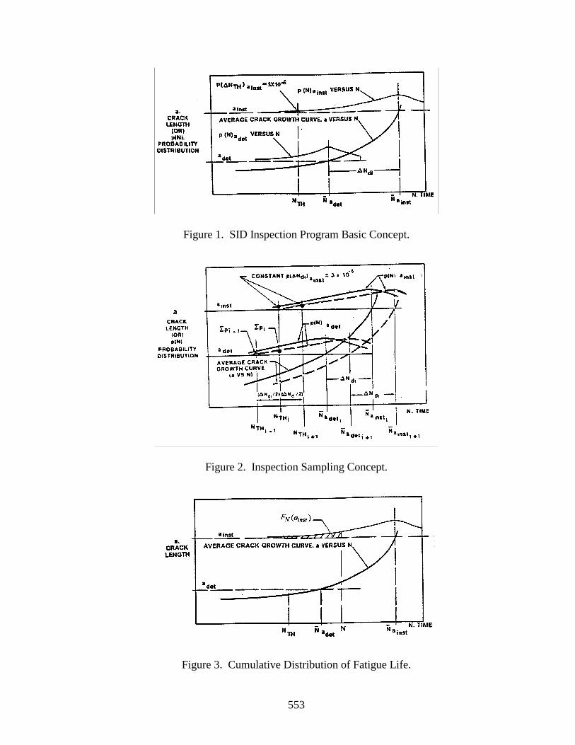
553
Figure 1. SID Inspection Program Basic Concept.
Figure 2. Inspection Sampling Concept.
Figure 3. Cumulative Distribution of Fatigue Life.
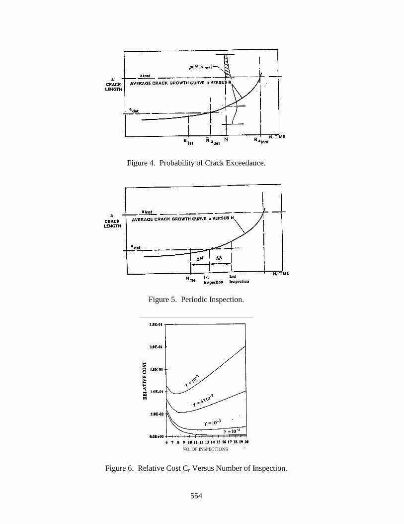
554
Figure 4. Probability of Crack Exceedance.
Figure 5. Periodic Inspection.
NO. OF INSPECTIONS
Figure 6. Relative Cost Cr Versus Number of Inspection.
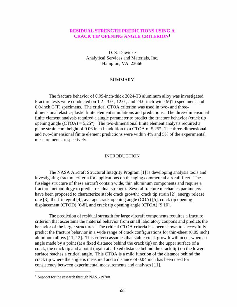
555
RESIDUAL STRENGTH PREDICTIONS USING ACRACK TIP OPENING ANGLE CRITERION 1
D. S. DawickeAnalytical Services and Materials, Inc.
Hampton, VA 23666
SUMMARY
The fracture behavior of 0.09-inch-thick 2024-T3 aluminum alloy was investigated.Fracture tests were conducted on 1.2-, 3.0-, 12.0-, and 24.0-inch-wide M(T) specimens and6.0-inch C(T) specimens. The critical CTOA criterion was used in two- and three-dimensional elastic-plastic finite element simulations and predictions. The three-dimensionalfinite element analysis required a single parameter to predict the fracture behavior (crack tipopening angle (CTOA) = 5.25°). The two-dimensional finite element analysis required aplane strain core height of 0.06 inch in addition to a CTOA of 5.25°. The three-dimensionaland two-dimensional finite element predictions were within 4% and 5% of the experimentalmeasurements, respectively.
INTRODUCTION
The NASA Aircraft Structural Integrity Program [1] is developing analysis tools andinvestigating fracture criteria for applications on the aging commercial aircraft fleet. Thefuselage structure of these aircraft contain wide, thin aluminum components and require afracture methodology to predict residual strength. Several fracture mechanics parametershave been proposed to characterize stable crack growth: crack tip strain [2], energy releaserate [3], the J-integral [4], average crack opening angle (COA) [5], crack tip openingdisplacement (CTOD) [6-8], and crack tip opening angle (CTOA) [9,10].
The prediction of residual strength for large aircraft components requires a fracturecriterion that ascertains the material behavior from small laboratory coupons and predicts thebehavior of the larger structures. The critical CTOA criteria has been shown to successfullypredict the fracture behavior in a wide range of crack configurations for thin-sheet (0.09 inch)aluminum alloys [11, 12]. This criteria assumes that stable crack growth will occur when anangle made by a point (at a fixed distance behind the crack tip) on the upper surface of acrack, the crack tip and a point (again at a fixed distance behind the crack tip) on the lowersurface reaches a critical angle. This CTOA is a mild function of the distance behind thecrack tip where the angle is measured and a distance of 0.04 inch has been used forconsistency between experimental measurements and analyses [11]. 1 Support for the research through NAS1-19708
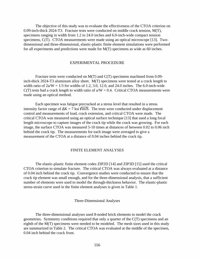
556
The objective of this study was to evaluate the effectiveness of the CTOA criterion on0.09-inch-thick 2024-T3. Fracture tests were conducted on middle crack tension, M(T),specimens ranging in width from 1.2 to 24.0 inches and 6.0-inch-wide compact tensionspecimens, C(T). CTOA measurements were made using an optical microscope [13]. Two-dimensional and three-dimensional, elastic-plastic finite element simulations were performedfor all experiments and predictions were made for M(T) specimens as wide as 60 inches.
EXPERIMENTAL PROCEDURE
Fracture tests were conducted on M(T) and C(T) specimens machined from 0.09-inch-thick 2024-T3 aluminum alloy sheet. M(T) specimens were tested at a crack length towidth ratio of 2a/W = 1/3 for widths of 1.2, 3.0, 12.0, and 24.0 inches. The 6.0-inch-wideC(T) tests had a crack length to width ratio of a/W = 0.4. Critical CTOA measurements weremade using an optical method.
Each specimen was fatigue precracked at a stress level that resulted in a stressintensity factor range of ∆K = 7 ksi inch. The tests were conducted under displacementcontrol and measurements of load, crack extension, and critical CTOA were made. Thecritical CTOA was measured using an optical surface technique [13] that used a long focallength microscope to capture images of the crack tip while the crack was growing. For eachimage, the surface CTOA was measured 5-10 times at distances of between 0.02 to 0.06 inchbehind the crack tip. The measurements for each image were averaged to give ameasurement of the CTOA at a distance of 0.04 inches behind the crack tip.
FINITE ELEMENT ANALYSES
The elastic-plastic finite element codes ZIP2D [14] and ZIP3D [15] used the criticalCTOA criterion to simulate fracture. The critical CTOA was always evaluated at a distanceof 0.04 inch behind the crack tip. Convergence studies were conducted to ensure that thecrack tip element was small enough, and for the three-dimensional analysis, that a sufficientnumber of elements were used to model the through-thickness behavior. The elastic-plasticstress-strain curve used in the finite element analyses is given in Table 1.
Three-Dimensional Analyses
The three-dimensional analyses used 8-noded brick elements to model the crackgeometries. Symmetry conditions required that only a quarter of the C(T) specimens and aneighth of the M(T) specimens were needed to be modeled. The mesh sizes used in this studyare summarized in Table 2. The critical CTOA was evaluated at the middle of the specimen,0.04 inch behind the crack front.
557
Two convergence studies were conducted to determine the minimum element sizealong the crack plane and the number of elements required to model the thickness. First, twoM(T) meshes were created with crack-plane element sizes of 0.04 and 0.02 inch (the formerrequired that the CTOA be analyzed at the first node behind the crack tip and the latterrequired it to be analyzed at the second node behind the crack tip). Both meshes modeled thehalf thickness with a single layer of elements. The two analyses produced nearly the sameapplied load at failure, indicating that convergence was achieved. Thus, the 0.04 inchelement size (with CTOA evaluated at the first node behind the crack tip) was chosen for thethree-dimensional analyses.
For the second convergence study, the half thickness was modeled with one, two, andthree elements. The failure load of the two-layer model was slightly larger than the one-layermodel and was nearly the same as the three-layer model, as shown in Figure 1. Thisindicates that convergence was achieved with two or more layers, thus, the half thickness wasmodeled with two-layers for all of the three-dimensional analyses.
Two-Dimensional Analyses
The two-dimensional analysis used 3-noded constant strain triangular elements.Symmetry conditions required that only a quarter of the M(T) specimens and half of the C(T)specimens were needed to be modeled. The mesh sizes used in this study are summarized inTable 3. The critical CTOA was evaluated 0.04 inch behind the crack tip.
Four meshes were developed with crack tip element sizes of 0.04, 0.02, 0.01 and0.005 inch (evaluating the critical CTOA an the 1st, 2nd, 4th, and 8th node behind the cracktip, respectively) for M(T) specimen widths of 1.2, 3.0, 6.0, 12.0, and 24.0 inches. For eachmesh, an elastic-plastic finite element analysis was conducted under plane stress conditionsand a critical CTOA of 5.25° was used to simulate the fracture behavior. The critical stressesfrom the analyses are shown in Figure 2. The smaller specimens required smaller elementsizes to achieve convergence, while the 12.0- and 24.0-inch-wide specimen exhibited verylittle influence of mesh size. To balance the convergence requirements of the smallerspecimens and the computer resources required to analyze the larger specimens, the two-dimensional meshes used in this study all had the 0.02 inch crack tip elements.
The finite element analyses were conducted for plane strain and plane stressconditions and using a plane strain core. The plane strain core analyses forced a core ofelements along the crack plane to be under plane strain conditions while the rest of thespecimen was under plane stress conditions, as illustrated in Figure 3. The plane strain corewas intended to approximate the three-dimensional constraint that develops at the crack tip[16]. The height of the plane strain core (PSC) generally increases with specimen thicknessand was obtained through comparison with three-dimensional analyses.
558
RESULTS AND DISCUSSION
Fracture tests were conducted on the 0.09-inch-thick 2024-T3 aluminum alloy in bothM(T) and C(T) configurations. An optical technique was used to measure the critical CTOAat the surface. Two- and three-dimensional, elastic-plastic finite element analyses wereconducted to simulate the fracture experiments.
Critical CTOA Measurements
The surface CTOA measurements were made during fracture testing of the 3.0-,12.0-, and 24.0-inch-wide M(T) and 6.0-inch-wide C(T) specimens, as shown in Figures 4aand 4b [15, 17]. The trends of the surface CTOA values indicate that: (1) initially the CTOAwas high and decreased during a transient period, (2) after a small amount of stable crackgrowth, the CTOA oscillated about a constant value, (3) the scatter in the measurements wasas about ±1°, (4) the CTOA behavior of the different sized M(T) specimens and the C(T)specimen were identical, and (5) the average CTOA for all of the measurements after thetransient region was about 5.5°.
Finite Element Analyses
Three-dimensional, elastic-plastic finite element analyses were conducted for eachfracture test. Fracture simulations were performed for C(T) specimens ranging in width from2.0 to 8.0 inches. The critical CTOA required for the analysis to match the critical load ofthe 6.0 inch C(T) fracture test was 5.25°, as shown in Figure 5. This CTOA value was thenused to predict the fracture behavior of the 1.2- to 24.0-inch-wide M(T) tests, as shown inFigure 6. The M(T) finite element predictions were all within 4% of the experimentalmeasurements. The critical CTOA of 5.25° was within the scatter band and slightly belowthe mean of the experimental surface measurements.
The critical CTOA (5.25°) determined by the three-dimensional finite elementanalyses was used to predict fracture in two-dimensional analyses. Plane stress and planestrain analyses were conducted for both the C(T) and M(T) fracture tests, as shown in Figures7 and 8 respectively. Neither plane stress nor plane strain analyses were able to predict theexperimental measurements. The plane strain predictions overpredicted the critical stress ofthe smaller specimens and underpredicted the larger specimens. The plane stress predictionswere reversed from the plane strain, underpredicting the critical stress of the smallerspecimens and overpredicting the larger specimens. The difference between the plane stressand plane strain predictions were greatest for the large specimens, diverging as specimen sizeincreased. Two- and three-dimensional finite element predictions were performed for M(T)specimens up to 60.0 inches wide. For the 60.0-inch-wide M(T), the plane stress analysis
559
overpredicted and the plane strain analysis underpredicted the three-dimensional criticalstress by 13% and 38%, respectively.
The plane strain core concept was used to approximate the through-thicknessconstraint in a two-dimensional finite element analysis. A plane strain core height of PSC =0.06 inch was determined to best fit the experimental measurements, as shown by the dashedline in Figures 7 and 8. The two-dimensional predictions using the plane strain core werewithin 3% of the experimental measurements from the M(T) fracture tests and about 5%below the measured critical stress of the 6.0-inch-wide C(T) test. The C(T) predictions wereconsistently about 5% below the three-dimensional fracture predictions for specimen widthsranging from 2.0 to 8.0 inches.
CONCLUDING REMARKS
The fracture behavior of 0.09-inch-thick, 2024-T3 aluminum alloy was investigated.Fracture tests were conducted on 1.2-, 3.0-, 12.0-, and 24.0-inch-wide M(T) specimens and6.0-inch C(T) specimens. The critical CTOA criteria was used in two- and three-dimensionalelastic-plastic finite element simulations and predictions. The three-dimensional finiteelement analysis required a single parameter to predict the fracture behavior (CTOA = 5.25°).The two-dimensional finite element analysis required a plane strain core height of 0.06 inch.The results from this study indicate:
1. The three-dimensional finite element analyses required a critical CTOA of 5.25° tosimulate the fracture behavior of the 6.0-inch-wide C(T) specimens. This angle waswithin the scatter band and slightly below the mean of the experimental surfacemeasurements.
2. The critical CTOA required to match the 6.0-inch-wide C(T) was used to predict the
fracture behavior of the M(T) specimens. These predictions were within 4% of theexperimental measurements for specimens ranging in width from 1.2 to 24.0 inches.
3. The two-dimensional plane strain and plane stress analyses were as much as 10%
different from the experimental measurements and did not follow the trends of themeasurements. Furthermore, the three-dimensional analysis indicates that planestress and plane strain predictions would become worse as the specimen sizeincreases.
4. A plane strain core height of PSC = 0.06 inch was required for the two-dimensional
analyses to match the measured fracture behavior and the three-dimensional fracturepredictions for large specimen sizes. These predictions were within 5% of theexperimental measurements.
560
ACKNOWLEDGMENTS
This work was supported under the NASA Langley Research Center’s AircraftStructural Integrity Program, contract number NAS1-19708.
REFERENCES
1. Harris, C. E., “NASA Aircraft Structural Integrity Program,” NASA TM-102637,April 1990.
2. Orowan, E., “Fracture and Strength of Solids,” Report of Progress in Physics,Physical Society of London, Vol. 12, pp. 185-233, 1949.
3. Broberg, K. B., “On Stable Crack Growth,” Journal of the Mechanics and Physics ofSolids, Vol. 23, 1975, pp. 215-237.
4. Rice, J. R., “A Path Independent Integral and the Approximate Analysis of StrainConcentration by Notches and Cracks,” ASME Journal of Applied Mechanics, Vol.35, 1968, pp. 368-379.
5. Kanninen, M. F., “The Analysis of Stable Crack Growth in Type 304 Stainless Steel,”in Proceedings of the International Conference of Fracture, pp. 1759-1768 (1980).
6. Wells, A. A., “Unstable Crack Propagation in Metals: Cleavage and Fast Fracture,” inProceedings of the Cranfield Crack Propagation Symposium, Vol. 1, 1961, pp. 210-230.
7. Wells, A. A., “Application of Fracture Mechanics at and Beyond General Yielding,”British Welding Journal, Vol. 11, 1961, pp. 563-570.
8. Wells, A. A., “Notched Bar Tests, Fracture Mechanics and Brittle Strengths ofWelded Structures,” British Welding Journal, Vol. 12, 1963, pp. 2-13.
9. Anderson, H., “Finite Element Representation of Stable Crack Growth,” Journal ofMechanics and Physics of Solids, Vol. 21, 1973, pp. 337-356.
10. de Koning, A. U., “A Contribution to the Analysis of Quasi Static Crack Growth inSteel Materials,” in Fracture 1977, Proceedings of the 4th International Conference onFracture, Vol. 3, pp. 25-31.
11. Dawicke, D. S., Newman, J. C., Jr., Sutton, M. A., and Amstutz, B. E., “Influence ofCrack History on the Stable Tearing Behavior of a Thin-Sheet Material with MultipleCracks,” NASA Conference Publication 3274, pp. 193-212, September 1994.
561
12. Newman, J. C., Jr. and Dawicke, D. S., “Fracture Analysis of Stiffened Panels UnderBiaxial Loading with Widespread Cracking,” AGARD-CP-568, pp. 3-1 - 3-16,December 1995.
13. Dawicke, D. S. and Sutton, M. A., “Crack Tip Opening Angle Measurements andCrack Tunneling Under Stable Tearing in a Thin Sheet 2024-T3 Aluminum Alloy,NASA-CR 191523, September 1993.
14. Newman, J. C., Jr., “Finite-Element Analyses of Fatigue Crack Propagation--Including the Effects of Crack Closure,” Ph.D. Thesis, Virginia Polytechnic Instituteand State University, Blacksburg, VA, May 1974.
15. Shivakumar, K. N. and Newman, J. C., Jr., “ZIP3D - An Elastic and Elastic-PlasticFinite-Element Analysis Program for Cracked Bodies,” NASA TM-102753, 1990.
16. Hom, C. L. and McMeeking, R. M., “Large Crack Tip Opening in Thin, Elastic-Plastic Sheets,” International Journal of Fracture, Vol. 45, pp. 103-122, 1980.
17. Sutton, M. A., Dawicke, D. S., and Newman, J. C., Jr., “Orientation Effects on theMeasurement and Analysis of Critical CTOA in an Aluminum Alloy Sheet,” FractureMechanics: 26th Volume, ASTM STP 1256, W. G. Reuter, J. H. Underwood, and J.C. Newman, Jr., Eds., American Society for Testing and Materials, Philadelphia,1995.
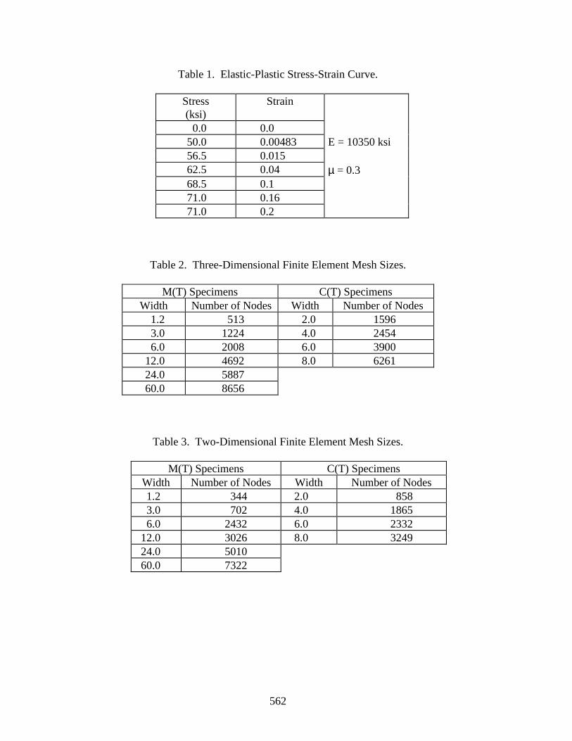
562
Table 1. Elastic-Plastic Stress-Strain Curve.
Stress(ksi)
Strain
0.0 0.050.0 0.00483 E = 10350 ksi56.5 0.01562.5 0.04 µ = 0.368.5 0.171.0 0.1671.0 0.2
Table 2. Three-Dimensional Finite Element Mesh Sizes.
M(T) Specimens C(T) SpecimensWidth Number of Nodes Width Number of Nodes
1.2 513 2.0 15963.0 1224 4.0 24546.0 2008 6.0 3900
12.0 4692 8.0 626124.0 588760.0 8656
Table 3. Two-Dimensional Finite Element Mesh Sizes.
M(T) Specimens C(T) SpecimensWidth Number of Nodes Width Number of Nodes1.2 344 2.0 8583.0 702 4.0 18656.0 2432 6.0 2332
12.0 3026 8.0 324924.0 501060.0 7322
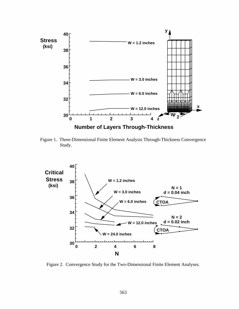
563
Number of Layers Throu gh-Thickness
Stress (ksi)
30
32
34
36
38
40
0 1 2 3 4
W = 1.2 inch
W = 3.0 inch
W = 6.0 inch
W = 12.0 inch
y
x
zW 2
Figure 1. Three-Dimensional Finite Element Analysis Through-Thickness ConvergenceStudy.
N
Critical Stress
(ksi)
30
32
34
36
38
40
0 2 4 6 8
W = 1.2 inch
W = 3.0 inch
W = 6.0 inch
W = 12.0 inch
W = 24.0 inch
N = 1 d = 0.04 inch
N = 2 d = 0.02 inch
CTOA
CTOA
Figure 2. Convergence Study for the Two-Dimensional Finite Element Analyses.
W = 1.2 inches
W = 3.0 inches
W = 6.0 inches
W = 12.0 inches
W = 1.2 inches
W = 3.0 inches
W = 6.0 inches
W = 12.0 inches
W = 24.0 inches
Stress(ksi)
Number of Layers Through-Thickness
CriticalStress
(ksi)
N
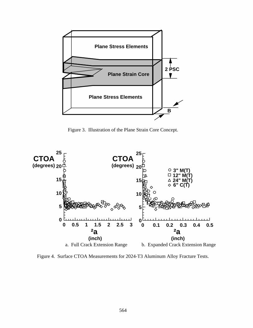
564
Plane Strain Core
Plane Stress Elements
Plane Stress Elements
B
2 PSC
Figure 3. Illustration of the Plane Strain Core Concept.
CTOA (degrees)
²a (inch)
CTOA (degrees)
²a (inch)
3" M(T)12" M(T)24" M(T)6" C(T)
0
5
10
15
20
25
0 0.1 0.2 0.3 0.4 0.50
5
10
15
20
25
0 0.5 1 1.5 2 2.5 3
a. Full Crack Extension Range b. Expanded Crack Extension Range
Figure 4. Surface CTOA Measurements for 2024-T3 Aluminum Alloy Fracture Tests.
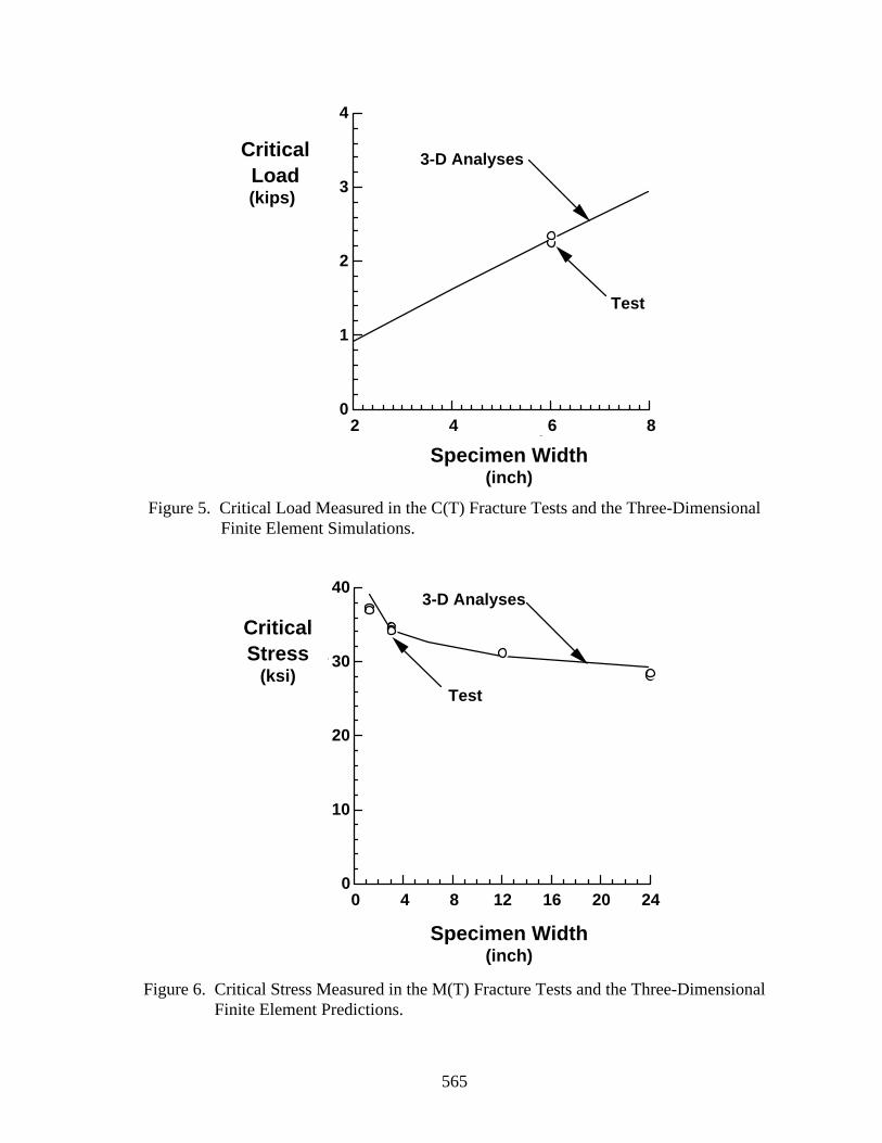
565
Specimen Width (inch)
Test
3-D Analyses
0
1
2
3
4
2 4 6 8
Critical Load (kips)
Figure 5. Critical Load Measured in the C(T) Fracture Tests and the Three-DimensionalFinite Element Simulations.
0
10
20
30
40
0 4 8 12 16 20 24
Specimen Width (inch)
Test
3-D Analyses
Critical Stress
(ksi)
Figure 6. Critical Stress Measured in the M(T) Fracture Tests and the Three-DimensionalFinite Element Predictions.
CriticalLoad(kips)
Specimen Width(inch)
CriticalStress
(ksi)
Specimen Width(inch)
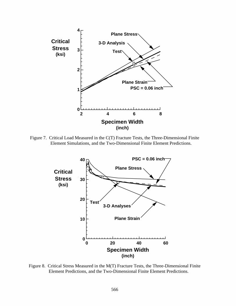
566
0
1
2
3
4
2 4 6 8
Specimen Width (inch)
Test
3-D AnalysisCritical Load (kips)
Plane Stress
Plane StrainPSC = 0.06 inch
Figure 7. Critical Load Measured in the C(T) Fracture Tests, the Three-Dimensional FiniteElement Simulations, and the Two-Dimensional Finite Element Predictions.
0
10
20
30
40
0 20 40 60Specimen Width
(inch)
Test3-D Analyses
Critical Stress
(ksi)
Plane Stress
Plane Strain
PSC = 0.06 inch
Figure 8. Critical Stress Measured in the M(T) Fracture Tests, the Three-Dimensional FiniteElement Predictions, and the Two-Dimensional Finite Element Predictions.
CriticalStress
(ksi)
Specimen Width(inch)
CriticalStress
(ksi)
Specimen Width(inch)
567
A REVIEW OF ROTORCRAFT STRUCTURAL INTEGRITY/AIRWORTHINESS APPROACHES AND ISSUES
Dr. Daniel P. SchrageCenter of Excellence in Rotorcraft Technology (CERT)
Codirector, Aerospace Systems Design Laboratory (ASDL)School of Aerospace EngineeringGeorgia Institute of Technology
Atlanta, GA 30332-0150
ABSTRACT
Rotorcraft are versatile machines that perform a variety of civil and military missions,thereby making fleet usage often difficult to track. Because the rotor system(s) and otherdynamic components are sized and designed principally on oscillatory loads, fatigue analysisand component tests form a substantial part and cost of a development program. While thefixed-wing community has moved from a safe-life (1950s) to fail-safe (1960s) to damagetolerant (1970s) structural design philosophy for the entire aircraft, many rotorcraft dynamiccomponent lives are still calculated using a safe-life design approach. This conservativeapproach is principally due to the uncertainty in rotor loads prediction in both the low- andhigh-speed flight regime. The fact that rotorcraft have virtually six degrees of freedommaneuverability capability in low speed provides incomparable agility (to fixed-wing aircraft),but complicates flight envelope definition and provides an extremely complex multidisciplinaryenvironment and unique interactions with the environment (terrain, earth boundary layerturbulence, wake induced from obstacles, etc.). In the relatively high-speed flight regime (-120 to 180 knots for helicopters) the aerodynamic load gradient across the main rotor disktranscends the entire subsonic, and a substantial portion of the transonic, regime (machnumber 0 to 0.95). Stalling on the retreating blade side of the main rotor disk andcompressibility on the advancing blade side produces extreme complications for rotor loadsprediction. Military helicopters in the past have included ballistic damage tolerant and fail-safedesign approaches, and new military rotorcraft developments, the V-22 Tilt Rotor Aircraft(Osprey) and the RAH-66 Conventional Helicopter (Comanche), are taking more of an overalldamage tolerant and fail-safe approach. However, a piecemeal structural design philosophy isstill being used for most rotorcraft and active research, although at a low level, has beenongoing to move to a more integrated structural design philosophy. Army, Air Force, Navy,the National Aeronautics and Space Administration (NASA), and the Federal AviationAdministration (FAA) have all had small efforts without any coordinated, sustained effort.The Army has had several false starts at initiating a Helicopter Structural Integrity Program(HSIP). The Air Force has supported efforts to apply the fixed wing damage toleranceapproach (ASIP) to its special operations helicopters. The Navy has developed a structuralmonitoring system based on the regime recognition concept for fatigue tracking of individualdynamic components. NASA has continued a low level effort to develop fracture mechanics
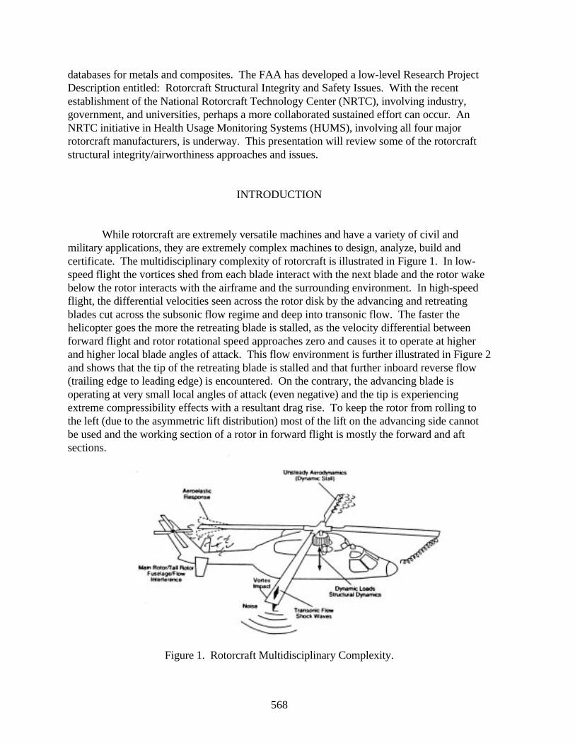
568
databases for metals and composites. The FAA has developed a low-level Research ProjectDescription entitled: Rotorcraft Structural Integrity and Safety Issues. With the recentestablishment of the National Rotorcraft Technology Center (NRTC), involving industry,government, and universities, perhaps a more collaborated sustained effort can occur. AnNRTC initiative in Health Usage Monitoring Systems (HUMS), involving all four majorrotorcraft manufacturers, is underway. This presentation will review some of the rotorcraftstructural integrity/airworthiness approaches and issues.
INTRODUCTION
While rotorcraft are extremely versatile machines and have a variety of civil andmilitary applications, they are extremely complex machines to design, analyze, build andcertificate. The multidisciplinary complexity of rotorcraft is illustrated in Figure 1. In low-speed flight the vortices shed from each blade interact with the next blade and the rotor wakebelow the rotor interacts with the airframe and the surrounding environment. In high-speedflight, the differential velocities seen across the rotor disk by the advancing and retreatingblades cut across the subsonic flow regime and deep into transonic flow. The faster thehelicopter goes the more the retreating blade is stalled, as the velocity differential betweenforward flight and rotor rotational speed approaches zero and causes it to operate at higherand higher local blade angles of attack. This flow environment is further illustrated in Figure 2and shows that the tip of the retreating blade is stalled and that further inboard reverse flow(trailing edge to leading edge) is encountered. On the contrary, the advancing blade isoperating at very small local angles of attack (even negative) and the tip is experiencingextreme compressibility effects with a resultant drag rise. To keep the rotor from rolling tothe left (due to the asymmetric lift distribution) most of the lift on the advancing side cannotbe used and the working section of a rotor in forward flight is mostly the forward and aftsections.
Figure 1. Rotorcraft Multidisciplinary Complexity.
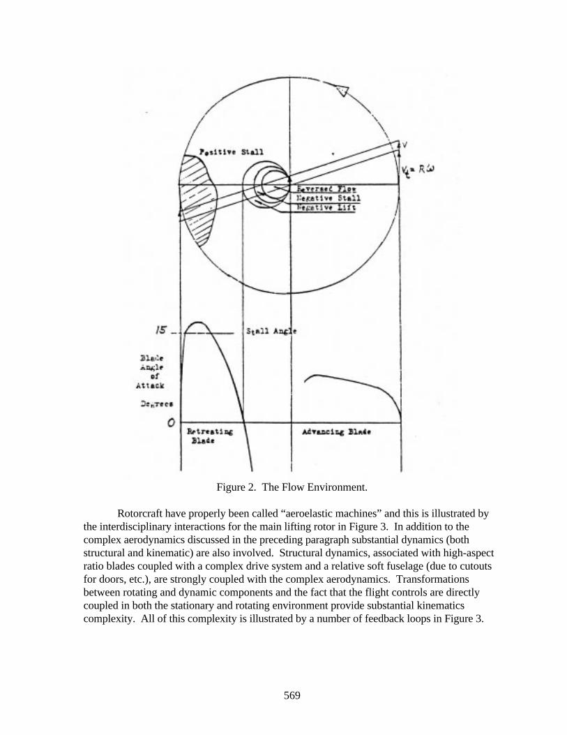
569
Figure 2. The Flow Environment.
Rotorcraft have properly been called “aeroelastic machines” and this is illustrated bythe interdisciplinary interactions for the main lifting rotor in Figure 3. In addition to thecomplex aerodynamics discussed in the preceding paragraph substantial dynamics (bothstructural and kinematic) are also involved. Structural dynamics, associated with high-aspectratio blades coupled with a complex drive system and a relative soft fuselage (due to cutoutsfor doors, etc.), are strongly coupled with the complex aerodynamics. Transformationsbetween rotating and dynamic components and the fact that the flight controls are directlycoupled in both the stationary and rotating environment provide substantial kinematicscomplexity. All of this complexity is illustrated by a number of feedback loops in Figure 3.
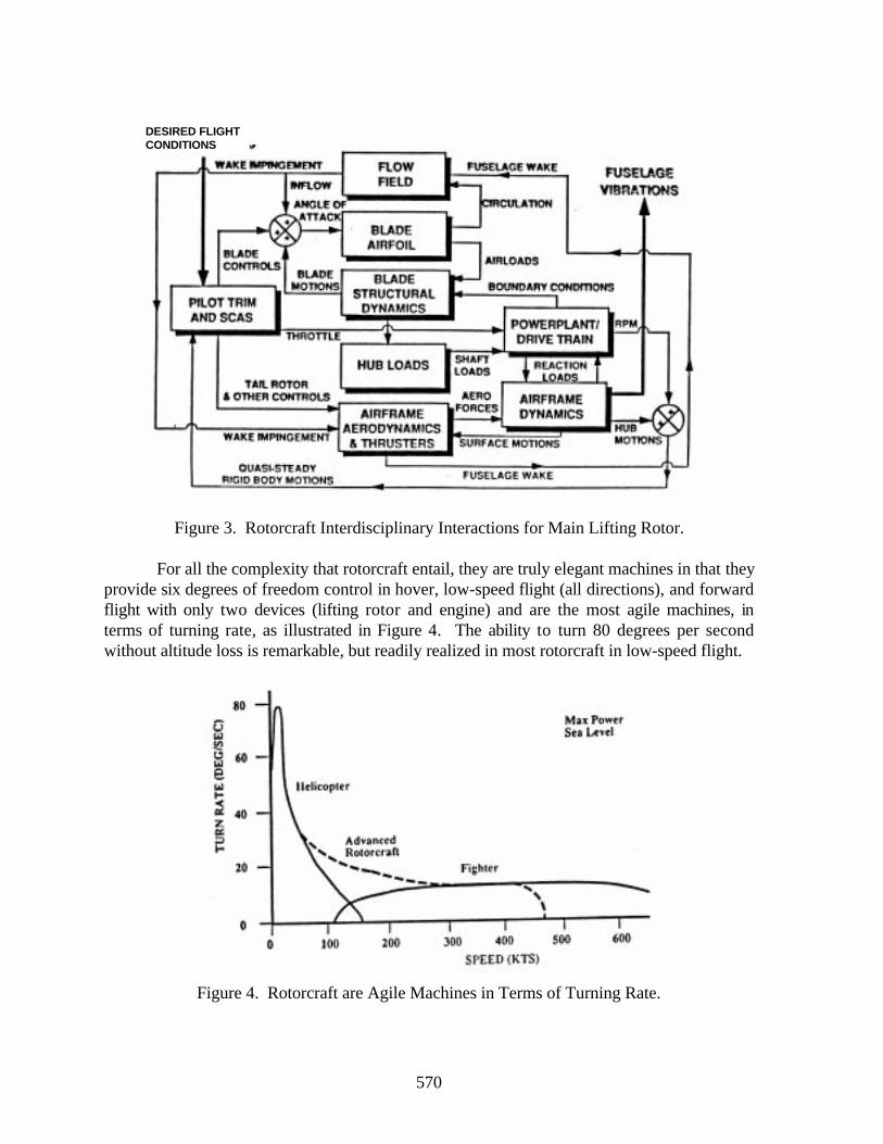
570
Figure 3. Rotorcraft Interdisciplinary Interactions for Main Lifting Rotor.
For all the complexity that rotorcraft entail, they are truly elegant machines in that theyprovide six degrees of freedom control in hover, low-speed flight (all directions), and forwardflight with only two devices (lifting rotor and engine) and are the most agile machines, interms of turning rate, as illustrated in Figure 4. The ability to turn 80 degrees per secondwithout altitude loss is remarkable, but readily realized in most rotorcraft in low-speed flight.
Figure 4. Rotorcraft are Agile Machines in Terms of Turning Rate.
DESIRED FLIGHTCONDITIONS
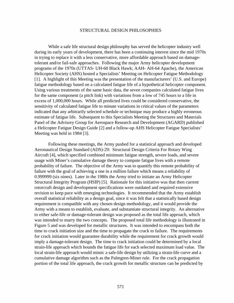
571
STRUCTURAL DESIGN PHILOSOPHIES
While a safe life structural design philosophy has served the helicopter industry wellduring its early years of development, there has been a continuing interest since the mid 1970sin trying to replace it with a less conservative, more affordable approach based on damage-tolerant and/or fail-safe approaches. Following the major Army helicopter developmentprograms of the 1970s (UTTAS- UH-60 Black Hawk; AAH- AH-64 Apache), the AmericanHelicopter Society (AHS) hosted a Specialists’ Meeting on Helicopter Fatigue Methodology[1]. A highlight of this Meeting was the presentation of the manufacturers’ (U.S. and Europe)fatigue methodology based on a calculated fatigue life of a hypothetical helicopter component.Using various treatments of the same basic data, the seven companies calculated fatigue livesfor the same component (a pitch link) with variations from a low of 745 hours to a life inexcess of 1,000,000 hours. While all predicted lives could be considered conservative, thesensitivity of calculated fatigue life to minute variations in critical values of the parametersindicated that any arbitrarily selected schedule or technique may produce a highly erroneousestimate of fatigue life. Subsequent to this Specialists Meeting the Structures and MaterialsPanel of the Advisory Group for Aerospace Research and Development (AGARD) publisheda Helicopter Fatigue Design Guide [2] and a follow-up AHS Helicopter Fatigue Specialists’Meeting was held in 1984 [3].
Following these meetings, the Army pushed for a statistical approach and developedAeronautical Design Standard (ADS)-29: Structural Design Criteria For Rotary WingAircraft [4], which specified combined minimum fatigue strength, severe loads, and severeusage with Miner’s cumulative damage theory to compute fatigue lives with a remoteprobability of failure. The objective of the Army was to quantify this remote probability offailure with the goal of achieving a one in a million failure which means a reliability of0.999999 (six nines). Later in the 1980s the Army tried to initiate an Army HelicopterStructural Integrity Program (HSIP) [5]. Rationale for this initiative was that then currentrotorcraft design and development specifications were outdated and required extensiverevision to keep pace with emerging technologies. It recommended that the Army establishoverall statistical reliability as a design goal, since it was felt that a statistically based designrequirement is compatible with any chosen design methodology, and it would provide theArmy with a means to establish, evaluate, and substantiate structural integrity. An alternativeto either safe-life or damage-tolerant design was proposed as the total life approach, whichwas intended to marry the two concepts. The proposed total life methodology is illustrated inFigure 5 and was developed for metallic structures. It was intended to encompass both thetime to crack initiation size and the time to propagate the crack to failure. The requirementsfor crack initiation would guarantee durability while the requirement for crack growth wouldimply a damage-tolerant design. The time to crack initiation could be determined by a localstrain-life approach which bounds the fatigue life for each selected maximum load value. Thelocal strain-life approach would mimic a safe-life design by utilizing a strain-life curve and acumulative damage algorithm such as the Palmgren-Miner rule. For the crack propagationportion of the total life approach, the crack growth for metallic structure can be predicted by
572
various models relating crack growth rates and the stress intensity factors [5]. While the totallife approach was proposed it has not been developed or implemented.
Figure 5. Flow Diagram of the Total Life Methodology.
While the Air Force has contracted with Sikorsky Aircraft and the Georgia TechResearch Institute(GTRI) to evaluate the practicality of using the Air Force’s AircraftStructural Integrity Program (ASIP) damage-tolerant approach for its special operationshelicopters (H-53 and H-60), no firm conclusions have been drawn that can be applied ingeneral or on new development programs. The Navy has developed a structural usagemonitoring system based on the regime recognition concept for fatigue tracking of individualdynamic components with the objectives of maximizing the safety, reliability, and readiness ofthe fleet in an environment of limited defense resources [6]. The first Structural DataRecording Set (SDRS) was installed in the AH-IW Cobra fleet in February 1993. Fiftyaircraft were equipped with SDRS and a total 3,400 flight hours of usage were required.Conclusions drawn from this Navy effort [6] were:
1. Helicopter component fatigue strength, usage, and component flight loads in eachregime can be modeled with a three-parameter Weibull distribution.
2. The incremental joint probability density function of a component failure due to three
independent variables (usage, load, and strength) can be numerically computed usingWeibull distribution parameters and the expression of cumulative probability densityfunction.

573
3. The reliability associated with each life can be accurately determined. Thecontribution of usage, load, and strength to six nines reliability can be identified.
4. The reliability associated with a life is a function of the approach with which it is
determined. The differences in methodology could result in as much as two ninesdifference in reliability prediction.
5. Additional work in evaluating each of the variables is necessary if an acceptable
reliability methodology is to be developed.
The FAA’s position is that damage-tolerant design is the only practical way todecrease the number of accidents involving fatigue failures in civilian aircraft [7]. The FAAhas also noted that if damage tolerance is only 50 percent effective, then the fatal fatigueaccident rate would be reduced by one-half. In 1995 the FAA started a Research ProjectInitiative (RPI) - Rotorcraft Structural Integrity and Safety Issues [8]. This RPI wascomposed of six tasks with the following industry sponsors:
1. Rotorcraft Health Usage Monitoring Systems (HUMS) Operational Development -Bell Helicopter Textron, Inc. and Petroleum Helicopters, Inc.
2. Teetering Rotor System Aircraft - Robinson Helicopter
3. Damage Tolerance Database and Application Methodology - To be determined (TBD)
4. Guidance Material for Replacing Existing Parts with Advanced Material Parts - TBD
5. Fly-By-Wire Certification Requirements - TBD
6. Crash Protection Airbag Application to Light Helicopters - Simula/Sikorsky Aircraft
Results from the first task were reported by Bell Helicopter Textron at the 52nd AHSAnnual Forum in Washington, DC [9]. Usage data, collected on a Bell Model 412 helicopterthat was equipped with a commercially available HUMS and operated by PetroleumHelicopters Inc. (PHI) under an independent flight trial program, was used to evaluate twousage monitoring techniques, flight condition recognition (FCR) and flight load synthesis(FLS). For the selected components that were analyzed, the results of the evaluationindicated a potential for extending retirement lives. This was due to the damage accumulationrate for the FCR and FLS techniques being slower (“slow clock”) than the current method ofusing actual flight hours as the basis for retirement times. Based on the mission flown for thisaircraft, which is transporting workcrews to offshore oil platforms, the flight hours chargedagainst retirement times could be reduced by 50 percent or greater. Thus the operator wouldgain a considerable payback in reduced maintenance costs due to extension of retirementintervals [9].
574
The use of HUMS on rotorcraft is seen as an excellent opportunity to improve safetywhile at the same time save on operations and support costs. HUMS activities for rotorcraftare taking place around the world. In Britain the Civil Aeronautics Authority (CAA) hassponsored trials to prove the technology. North Sea helicopter operators are equipping fleetswith HUMS and working groups have been active since 1986. Military applications forHUMS are also proceeding in the U.S. Navy and Army, and in the UK Ministry of Defense(MOD). The National Rotorcraft Technology Center (NRTC) in the U.S. is also supporting acost-shared HUMS Project with the Rotorcraft Industry Technology Association (RITA),which is made up of the four major U.S. rotorcraft companies. Also, an array of suppliers areoffering HUMS and HUMS-related capabilities.
CONCLUSIONS
Ensuring rotorcraft structural integrity/airworthiness is extremely complex and notalways appreciated, due to the relatively low static load flight envelope (~3g’s) forhelicopters, i.e., V-N diagram. However, the capability of rotorcraft to provide six degrees ofmaneuvering freedom in low-speed flight make them the most agile (in terms of turning rate)of aircraft. This capability also makes defining flight envelopes, both steady and transient,extremely difficult due to the aero-servoelastic complications of the problem. Structuraldesign philosophies for rotorcraft have evolved at a much slower rate than for fixed-wingaircraft, largely due to the inability to accurately predict the oscillatory loads and to trackcrack growth in a high cycle environment. The utility of rotorcraft and their usage in a varietyof environments also make tracking fleet usage and crack detection and growth extremelydifficult. Therefore, no single structural design philosophy, such as damage tolerance, hasbeen accepted. There are low-level efforts in industry and government to move toward anintegrated structural design philosophy/methodology, but no unified approach. One particularpromising technology for rotorcraft structural integrity and airworthiness is Health UsageMonitoring Systems (HUMS) which will allow the individual tracking of usage, provided itproves to be cost effective.
REFERENCES
1. Borgman, D. C. and Schrage, D. P.: “Synopsis of Specialists’ Meeting On HelicopterFatigue Methodology,” AGARD Conference Proceedings No. 297: HELICOPTERFATIGUE LIFE ASSESSMENT, 1981.
2. AGARD Helicopter Fatigue Design Guide, 1993. 3. AHS Midwest Region Helicopter Fatigue Specialists’ Meeting, St. Louis, MO,
October 16-18, 1984.

575/576
4. Structural Design Criteria For Rotary Wing Aircraft, Aeronautical Design Standard(ADS) - 29, United States Army Aviation Systems Command. St. Louis, MO,September 1986.
5. Spigel, B.: “Foundations of an Army Helicopter Structural Integrity Program,” AHS
National Specialists’ Meeting on Advanced Rotorcraft Structures, Williamsburg, VA,October 25-27, 1988.
6. Moon, S., Menon, D., and Barndt, G.: “Fatigue Life Reliability Based On Measured
Usage, Flight Loads and Fatigue Strength Variations,” Proceedings of the 52ndAnnual Forum of the AHS, Washington, DC, June 4-6, 1996.
7. Weaver, R. T.: “Damage Tolerance and Civil Helicopter Design,” AHS Specialists’
Meeting on Fatigue Methodology, St. Louis, MO, October 1984. 8. Federal Aviation Administration (FAA) Research Project Initiative (RPI) - Rotorcraft
Structural Integrity and Safety Issues, January 1995. 9. Dickson, W. and Cronkhite, J. D.: “Usage and Structural Life Monitoring with
HUMS,” Proceedings of the 52nd Annual Forum of the AHS, Washington, DC, June4-6, 1996.
577
RIVET BEARING LOAD CONSIDERATIONS IN THE DESIGN OFMECHANICAL REPAIRS FOR AGING AIRCRAFT 1
Hemant Chickermane and Hae Chang GeaDepartment of Mechanical and Aerospace Engineering
Rutgers, The State University of New JerseyPiscataway, NJ 08855
INTRODUCTION
Mechanical repairs of aging repairs need to be designed to restore the structure to itsoriginal or better structural integrity. Poor repairs give rise to a nonuniform distribution offorces across the doubler patch. The original details for service loadings may be changed andthereby adversely effect the fatigue life of the aircraft structure. Due to the load transferbetween aircraft skin and the repair doubler, fastener holes are subjected to bearing stresses.High stress concentrations at the rivet holes in the skin could lead to crack initiation andmultisite damage, which could be catastrophic. While the rivets themselves are subject toshear failure, it has been found that bearing failure at fastener joints predominates.
In the past a methodology was developed to generate designs for mechanical repairsbased on an energy criterion. This procedure determines optimal locations for rivets on thedoubler patch in a manner that minimizes the deformations in the structural systemcomprising the aircraft skin, doubler patch, and rivets. Repair designs were generated for avariety of repair configurations for different shapes of doublers and regions of rivetplacement. One concern that needs to be addressed is the possibility of localized high-stressregions in the vicinity of the rivets. In this work, the computation of bearing loads and theirincorporation into the repair design problem has been investigated. Emphasis is placed ongenerating repairs with greater stiffness without subjecting rivets to excessively large loads.
BACKGROUND
At present, the main criterion for the design of mechanical repairs is static strength.Swift [1] proposed one of the earliest models for aircraft repairs. It is a one-dimensionalmodel in which the skin and doubler are represented by axial rods and rivets by shear rods.An implicit assumption of this model is that load transfers in fasteners are uniform.However, a two-dimensional model is necessary to account for biaxial stresses and for greateraccuracy in calculation of load transfers. The researchers at Battelle (see Rice, et. al [2])extended the Swift model to two dimensions using spring-like discrete members connecting 1 This work was supported by a grant from the Federal Aviation Administration (FAA) through the Center forComputational Modeling of Aircraft Structures (CMAS) at Rutgers University
578
the fasteners in both principal axes with axial and shear stiffness terms. This wasimplemented in the form of an analysis code called SKINFIX.
Since most of the research in the field of aircraft repairs deals with analysis of repairs,the design of repairs depend on the skill and experience of the engineer. Therefore,Chickermane and Gea [3] proposed a systematic design methodology which integrates theanalysis of the repair with the redesign capability obtained by formulating it as anoptimization problem. A three-dimensional model has been used to analyze the repair.Aircraft skin and doubler are modeled by quadrilateral thin-shell elements and rivets by rigidlinear springs in three directions. The effect of a central crack in the skin is simulated bysubjecting the skin to in plane loads, perpendicular to the direction of the crack.
MAIN COMPONENTS OF THE METHODOLOGY
Formulation of an Optimization Problem
The objective of the repair design procedure is to locate the rivets on the doublerpatch in a way that minimizes the structural deformation. Since deformation is a localphenomenon, the location of the maximum displacement may vary from one design toanother leading to a discontinuous objective function. To avoid this problem, a globalmeasure of deformation of the structure in terms of the strain energy has been used.Therefore, the objective function is the mean compliance of the structure which is twice thestrain energy. The strategy employed here is to constrain the bearing stresses in aircraft skinand doubler by ensuring that the maximum bearing loads stay within limits. This would alsoensure a more uniform distribution of rivet loads. An upper limit is also placed on thenumber of rivets permitted.
Every rivet is modeled by rigid springs in three directions. The spring acting in thedirection of the external loading is responsible for the shear resistance of the rivet. The shearforce acting on the rivet is equal to the force exerted by the rivet on the doubler and skin isthe bearing load. Therefore, rivet bearing loads are calculated in the direction of the appliedskin loads. For a particular rivet i, bearing load transferred in direction j is
F k u uij ij ij ij= −( )1 2 (1)
where u ij1 and u ij2 are the doubler and skin displacements at the point of attachment
respectively and kij is the rivet stiffness. Rivets having the maximum bearing loads are
targeted and appropriate limits are placed on them based on results obtained from previousdesigns. The bearing load constraints are then introduced into the optimization problem asconstraints.
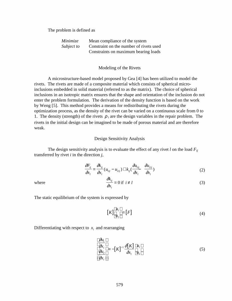
579
The problem is defined as
Minimize Mean compliance of the systemSubject to Constraint on the number of rivets used
Constraints on maximum bearing loads
Modeling of the Rivets
A microstructure-based model proposed by Gea [4] has been utilized to model therivets. The rivets are made of a composite material which consists of spherical micro-inclusions embedded in solid material (referred to as the matrix). The choice of sphericalinclusions in an isotropic matrix ensures that the shape and orientation of the inclusion do notenter the problem formulation. The derivation of the density function is based on the workby Weng [5]. This method provides a means for redistributing the rivets during theoptimization process, as the density of the rivet can be varied on a continuous scale from 0 to1. The density (strength) of the rivets ρ i are the design variables in the repair problem. Therivets in the initial design can be imagined to be made of porous material and are thereforeweak.
Design Sensitivity Analysis
The design sensitivity analysis is to evaluate the effect of any rivet l on the load Fij
transferred by rivet i in the direction j,
∂∂
∂∂
∂∂
∂∂
F
x
k
xu u k
u
x
u
xij
l
ij
lij ij ij
ij
l
ij
l
= − + −( ) ( )1 2
1 2(2)
where ∂∂k
xij
l
= 0 if i l≠ (3)
The static equilibrium of the system is expressed by
[ ] [ ]Ku
uF
1
2
= (4)
Differentiating with respect to xl and rearranging
[ ] [ ]∂∂∂∂
∂∂
u
xu
x
KK
x
u
ul
l
l
1
2
1 1
2
= −
− (5)
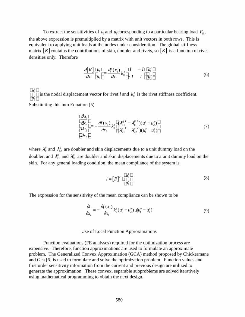
580
To extract the sensitivities of u1 and u2corresponding to a particular bearing load Fij ,
the above expression is premultiplied by a matrix with unit vectors in both rows. This isequivalent to applying unit loads at the nodes under consideration. The global stiffnessmatrix [ ]K contains the contributions of skin, doubler and rivets, so [ ]K is a function of rivetdensities only. Therefore
[ ]∂∂
∂∂
K
x
u
u
f x
xk
I I
I I
u
ul
i
l
ee
e
1
20
1
2
=
−−
( )(6)
u
u
e
e
1
2
is the nodal displacement vector for rivet l and ke
0 is the rivet stiffness coefficient.
Substituting this into Equation (5)
∂∂∂∂
∂∂
λ λλ λ
u
xu
x
f x
xk
u u
u ul
l
i
l
eij T ij T e e
ij T ij T e e
1
20
11 11 1 2
21 22 1 2
= −− −− −
( ) ( )( )
( )( )(7)
where λ11ij and λ12
ij are doubler and skin displacements due to a unit dummy load on the
doubler, and λ21ij and λ22
ij are doubler and skin displacements due to a unit dummy load on theskin. For any general loading condition, the mean compliance of the system is
[ ]l Fu
uT
e
e= ⋅
1
2
(8)
The expression for the sensitivity of the mean compliance can be shown to be
∂∂
∂∂
l
x
f x
xk u u u u
l
i
l
e e e e e= − − ⋅ −( )
( ) ( )0 1 2 1 2 (9)
Use of Local Function Approximations
Function evaluations (FE analyses) required for the optimization process areexpensive. Therefore, function approximations are used to formulate an approximateproblem. The Generalized Convex Approximation (GCA) method proposed by Chickermaneand Gea [6] is used to formulate and solve the optimization problem. Function values andfirst order sensitivity information from the current and previous design are utilized togenerate the approximation. These convex, separable subproblems are solved iterativelyusing mathematical programming to obtain the next design.
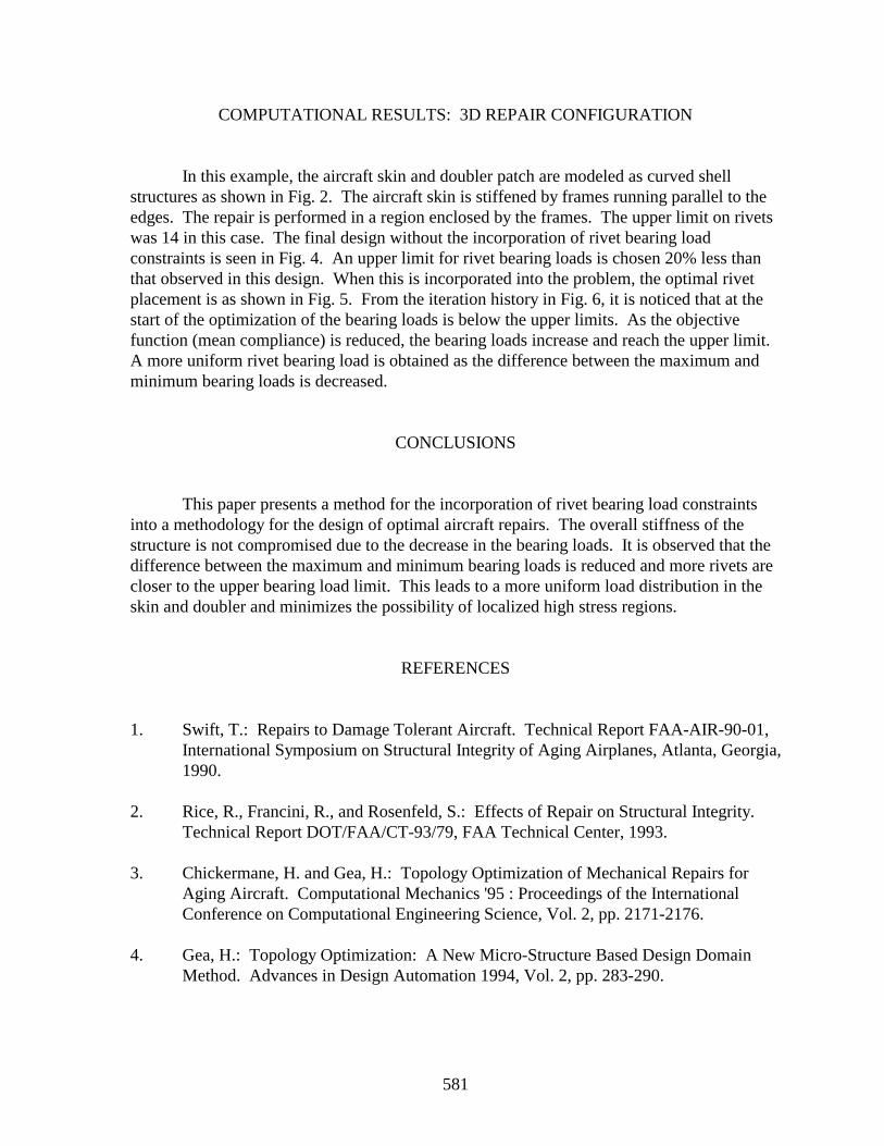
581
COMPUTATIONAL RESULTS: 3D REPAIR CONFIGURATION
In this example, the aircraft skin and doubler patch are modeled as curved shellstructures as shown in Fig. 2. The aircraft skin is stiffened by frames running parallel to theedges. The repair is performed in a region enclosed by the frames. The upper limit on rivetswas 14 in this case. The final design without the incorporation of rivet bearing loadconstraints is seen in Fig. 4. An upper limit for rivet bearing loads is chosen 20% less thanthat observed in this design. When this is incorporated into the problem, the optimal rivetplacement is as shown in Fig. 5. From the iteration history in Fig. 6, it is noticed that at thestart of the optimization of the bearing loads is below the upper limits. As the objectivefunction (mean compliance) is reduced, the bearing loads increase and reach the upper limit.A more uniform rivet bearing load is obtained as the difference between the maximum andminimum bearing loads is decreased.
CONCLUSIONS
This paper presents a method for the incorporation of rivet bearing load constraintsinto a methodology for the design of optimal aircraft repairs. The overall stiffness of thestructure is not compromised due to the decrease in the bearing loads. It is observed that thedifference between the maximum and minimum bearing loads is reduced and more rivets arecloser to the upper bearing load limit. This leads to a more uniform load distribution in theskin and doubler and minimizes the possibility of localized high stress regions.
REFERENCES
1. Swift, T.: Repairs to Damage Tolerant Aircraft. Technical Report FAA-AIR-90-01,International Symposium on Structural Integrity of Aging Airplanes, Atlanta, Georgia,1990.
2. Rice, R., Francini, R., and Rosenfeld, S.: Effects of Repair on Structural Integrity.
Technical Report DOT/FAA/CT-93/79, FAA Technical Center, 1993. 3. Chickermane, H. and Gea, H.: Topology Optimization of Mechanical Repairs for
Aging Aircraft. Computational Mechanics '95 : Proceedings of the InternationalConference on Computational Engineering Science, Vol. 2, pp. 2171-2176.
4. Gea, H.: Topology Optimization: A New Micro-Structure Based Design Domain
Method. Advances in Design Automation 1994, Vol. 2, pp. 283-290.
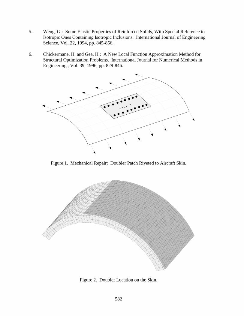
582
5. Weng, G.: Some Elastic Properties of Reinforced Solids, With Special Reference toIsotropic Ones Containing Isotropic Inclusions. International Journal of EngineeringScience, Vol. 22, 1994, pp. 845-856.
6. Chickermane, H. and Gea, H.: A New Local Function Approximation Method for
Structural Optimization Problems. International Journal for Numerical Methods inEngineering., Vol. 39, 1996, pp. 829-846.
Figure 1. Mechanical Repair: Doubler Patch Riveted to Aircraft Skin.
Figure 2. Doubler Location on the Skin.
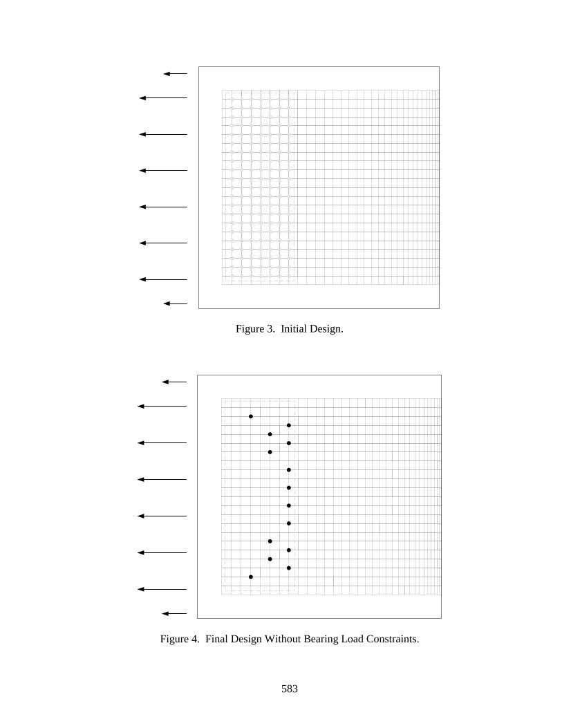
583
Figure 3. Initial Design.
Figure 4. Final Design Without Bearing Load Constraints.
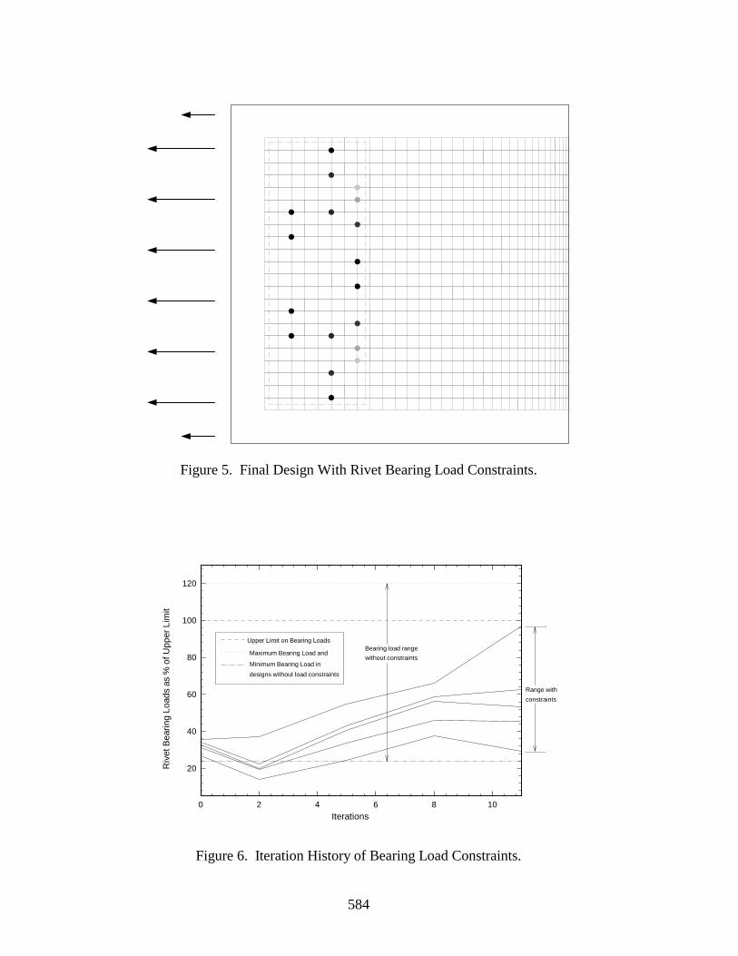
584
Figure 5. Final Design With Rivet Bearing Load Constraints.
0 5 10 15 2040
60
80
100
120
(2D) || Print || 25 Jul 1996 || plot1.plt ||
0 5 10 15 2040
60
80
100
120
(2D) || Print || 25 Jul 1996 || plot1.plt ||
0 2 4 6 8 10
20
40
60
80
0 2 4 6 8 10
20
40
60
80
100
120
Iterations
Riv
et B
earin
g Lo
ads
as %
of U
pper
Lim
it
Upper Limit on Bearing Loads
Minimum Bearing Load in
Maximum Bearing Load and
designs without load constraints
Bearing load range
without constraints
Range with
constraints
Figure 6. Iteration History of Bearing Load Constraints.
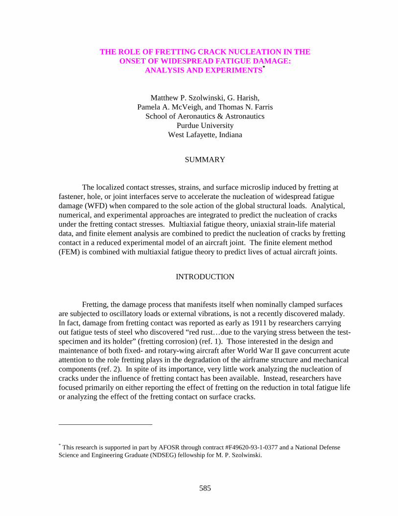
585
THE ROLE O F FRETTING CRACK NUCLEATION IN THEONSET OF WIDESPREAD FATIGUE DAMAGE:
ANALYSIS AND EXPERIMENTS *
Matthew P. Szolwinski, G. Harish,Pamela A. McVeigh, and Thomas N. Farris
School of Aeronautics & AstronauticsPurdue University
West Lafayette, Indiana
SUMMARY
The localized contact stresses, strains, and surface microslip induced by fretting atfastener, hole, or joint interfaces serve to accelerate the nucleation of widespread fatiguedamage (WFD) when compared to the sole action of the global structural loads. Analytical,numerical, and experimental approaches are integrated to predict the nucleation of cracksunder the fretting contact stresses. Multiaxial fatigue theory, uniaxial strain-life materialdata, and finite element analysis are combined to predict the nucleation of cracks by frettingcontact in a reduced experimental model of an aircraft joint. The finite element method(FEM) is combined with multiaxial fatigue theory to predict lives of actual aircraft joints.
INTRODUCTION
Fretting, the damage process that manifests itself when nominally clamped surfacesare subjected to oscillatory loads or external vibrations, is not a recently discovered malady.In fact, damage from fretting contact was reported as early as 1911 by researchers carryingout fatigue tests of steel who discovered “red rust…due to the varying stress between the test-specimen and its holder” (fretting corrosion) (ref. 1). Those interested in the design andmaintenance of both fixed- and rotary-wing aircraft after World War II gave concurrent acuteattention to the role fretting plays in the degradation of the airframe structure and mechanicalcomponents (ref. 2). In spite of its importance, very little work analyzing the nucleation ofcracks under the influence of fretting contact has been available. Instead, researchers havefocused primarily on either reporting the effect of fretting on the reduction in total fatigue lifeor analyzing the effect of the fretting contact on surface cracks.
* This research is supported in part by AFOSR through contract #F49620-93-1-0377 and a National DefenseScience and Engineering Graduate (NDSEG) fellowship for M. P. Szolwinski.
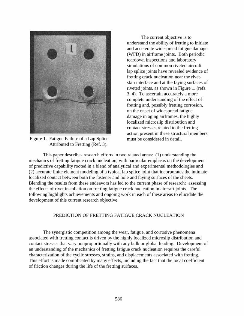
586
The current objective is tounderstand the ability of fretting to initiateand accelerate widespread fatigue damage(WFD) in airframe joints. Both periodicteardown inspections and laboratorysimulations of common riveted aircraftlap splice joints have revealed evidence offretting crack nucleation near the rivet-skin interface and at the faying surfaces ofriveted joints, as shown in Figure 1. (refs.3, 4). To ascertain accurately a morecomplete understanding of the effect offretting and, possibly fretting corrosion,on the onset of widespread fatiguedamage in aging airframes, the highlylocalized microslip distribution andcontact stresses related to the frettingaction present in these structural membersmust be considered in detail.
This paper describes research efforts in two related areas: (1) understanding themechanics of fretting fatigue crack nucleation, with particular emphasis on the developmentof predictive capability rooted in a blend of analytical and experimental methodologies and(2) accurate finite element modeling of a typical lap splice joint that incorporates the intimatelocalized contact between both the fastener and hole and faying surfaces of the sheets.Blending the results from these endeavors has led to the current phase of research: assessingthe effects of rivet installation on fretting fatigue crack nucleation in aircraft joints. Thefollowing highlights achievements and ongoing work in each of these areas to elucidate thedevelopment of this current research objective.
PREDICTION OF FRETTING FATIGUE CRACK NUCLEATION
The synergistic competition among the wear, fatigue, and corrosive phenomenaassociated with fretting contact is driven by the highly localized microslip distribution andcontact stresses that vary nonproportionally with any bulk or global loading. Development ofan understanding of the mechanics of fretting fatigue crack nucleation requires the carefulcharacterization of the cyclic stresses, strains, and displacements associated with fretting.This effort is made complicated by many effects, including the fact that the local coefficientof friction changes during the life of the fretting surfaces.
Figure 1. Fatigue Failure of a Lap SpliceAttributed to Fretting (Ref. 3).
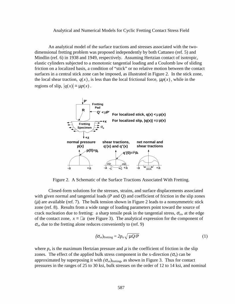
587
Analytical and Numerical Models for Cyclic Fretting Contact Stress Field
An analytical model of the surface tractions and stresses associated with the two-dimensional fretting problem was proposed independently by both Cattaneo (ref. 5) andMindlin (ref. 6) in 1938 and 1949, respectively. Assuming Hertzian contact of isotropic,elastic cylinders subjected to a monotonic tangential loading and a Coulomb law of slidingfriction on a localized basis, a condition of “stick” or no relative motion between the contactsurfaces in a central stick zone can be imposed, as illustrated in Figure 2. In the stick zone,the local shear traction, q x( ) , is less than the local frictional force, µp x( ) , while in the
regions of slip, q x p x( ) ( )= µ .
Figure 2. A Schematic of the Surface Tractions Associated With Fretting.
Closed-form solutions for the stresses, strains, and surface displacements associatedwith given normal and tangential loads (P and Q) and coefficient of friction in the slip zones(µ) are available (ref. 7). The bulk tension shown in Figure 2 leads to a nonsymmetric stickzone (ref. 8). Results from a wide range of loading parameters point toward the source ofcrack nucleation due to fretting: a sharp tensile peak in the tangential stress, σxx, at the edgeof the contact zone, x a= + (see Figure 3). The analytical expression for the component ofσxx due to the fretting alone reduces conveniently to (ref. 9)
(σxx)fretting = 2po µQ/P (1)
where po is the maximum Hertzian pressure and µ is the coefficient of friction in the slipzones. The effect of the applied bulk stress component in the x-direction (σo) can beapproximated by superposing it with (σxx)fretting, as shown in Figure 3. Thus for contactpressures in the ranges of 25 to 30 ksi, bulk stresses on the order of 12 to 14 ksi, and nominal
normal pressurep(x)
-a +a
shear tractions,q′(x) and q ″(x)
net normal andshear tractions
+a-a -c +c stick +a-a
P′Fretting
Pad
FrettingSpecimen
+x
+z
R Q′ < µP′
p(0)=po q′(0)=µpo
For localized stick, q(x) < µ p(x)
For localized slip, |q(x)| = µ p(x)
σo
slip slip
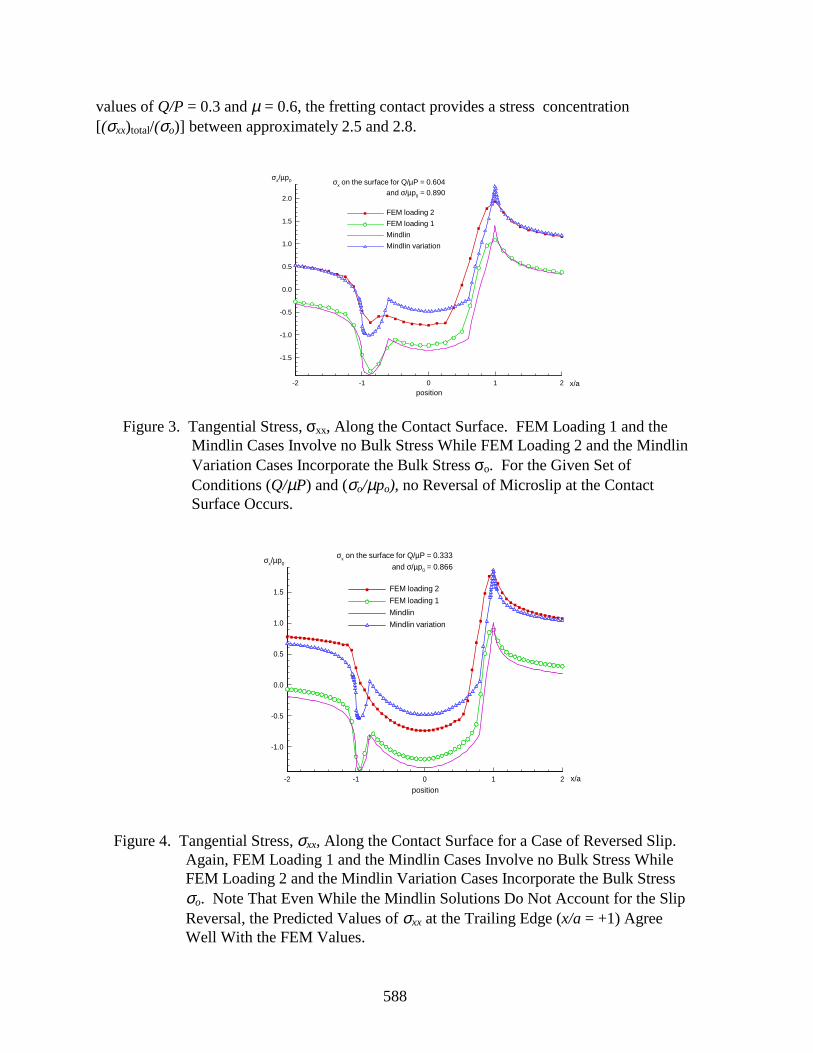
588
values of Q/P = 0.3 and µ = 0.6, the fretting contact provides a stress concentration[(σxx)total/(σo)] between approximately 2.5 and 2.8.
Figure 3. Tangential Stress, σxx, Along the Contact Surface. FEM Loading 1 and theMindlin Cases Involve no Bulk Stress While FEM Loading 2 and the MindlinVariation Cases Incorporate the Bulk Stress σo. For the Given Set ofConditions (Q/µP) and (σo/µpo), no Reversal of Microslip at the ContactSurface Occurs.
Figure 4. Tangential Stress, σxx, Along the Contact Surface for a Case of Reversed Slip.Again, FEM Loading 1 and the Mindlin Cases Involve no Bulk Stress WhileFEM Loading 2 and the Mindlin Variation Cases Incorporate the Bulk Stressσo. Note That Even While the Mindlin Solutions Do Not Account for the SlipReversal, the Predicted Values of σxx at the Trailing Edge (x/a = +1) AgreeWell With the FEM Values.
-2 -1 0 1 2
-1.5
-1.0
-0.5
0.0
0.5
1.0
1.5
2.0
σx/µp0
FEM loading 2
Mindlin
Mindlin variation
FEM loading 1
positionx/a
σx on the surface for Q/µP = 0.604and σ/µp0 = 0.890
-2 -1 0 1 2
-1.0
-0.5
0.0
0.5
1.0
1.5
σx/µp0
FEM loading 2
Mindlin variation
Mindlin
FEM loading 1
positionx/a
σx on the surface for Q/µP = 0.333and σ/µp0 = 0.866
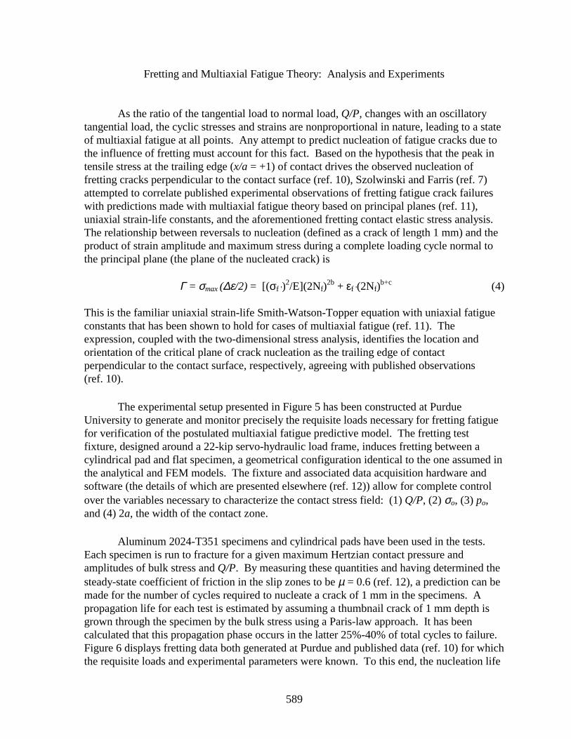
589
Fretting and Multiaxial Fatigue Theory: Analysis and Experiments
As the ratio of the tangential load to normal load, Q/P, changes with an oscillatorytangential load, the cyclic stresses and strains are nonproportional in nature, leading to a stateof multiaxial fatigue at all points. Any attempt to predict nucleation of fatigue cracks due tothe influence of fretting must account for this fact. Based on the hypothesis that the peak intensile stress at the trailing edge (x/a = +1) of contact drives the observed nucleation offretting cracks perpendicular to the contact surface (ref. 10), Szolwinski and Farris (ref. 7)attempted to correlate published experimental observations of fretting fatigue crack failureswith predictions made with multiaxial fatigue theory based on principal planes (ref. 11),uniaxial strain-life constants, and the aforementioned fretting contact elastic stress analysis.The relationship between reversals to nucleation (defined as a crack of length 1 mm) and theproduct of strain amplitude and maximum stress during a complete loading cycle normal tothe principal plane (the plane of the nucleated crack) is
Γ = σmax (∆ε/2) = [(σf ')2/E](2Nf)
2b + εf '(2Nf)b+c (4)
This is the familiar uniaxial strain-life Smith-Watson-Topper equation with uniaxial fatigueconstants that has been shown to hold for cases of multiaxial fatigue (ref. 11). Theexpression, coupled with the two-dimensional stress analysis, identifies the location andorientation of the critical plane of crack nucleation as the trailing edge of contactperpendicular to the contact surface, respectively, agreeing with published observations(ref. 10).
The experimental setup presented in Figure 5 has been constructed at PurdueUniversity to generate and monitor precisely the requisite loads necessary for fretting fatiguefor verification of the postulated multiaxial fatigue predictive model. The fretting testfixture, designed around a 22-kip servo-hydraulic load frame, induces fretting between acylindrical pad and flat specimen, a geometrical configuration identical to the one assumed inthe analytical and FEM models. The fixture and associated data acquisition hardware andsoftware (the details of which are presented elsewhere (ref. 12)) allow for complete controlover the variables necessary to characterize the contact stress field: (1) Q/P, (2) σo, (3) po,and (4) 2a, the width of the contact zone.
Aluminum 2024-T351 specimens and cylindrical pads have been used in the tests.Each specimen is run to fracture for a given maximum Hertzian contact pressure andamplitudes of bulk stress and Q/P. By measuring these quantities and having determined thesteady-state coefficient of friction in the slip zones to be µ = 0.6 (ref. 12), a prediction can bemade for the number of cycles required to nucleate a crack of 1 mm in the specimens. Apropagation life for each test is estimated by assuming a thumbnail crack of 1 mm depth isgrown through the specimen by the bulk stress using a Paris-law approach. It has beencalculated that this propagation phase occurs in the latter 25%-40% of total cycles to failure.Figure 6 displays fretting data both generated at Purdue and published data (ref. 10) for whichthe requisite loads and experimental parameters were known. To this end, the nucleation life
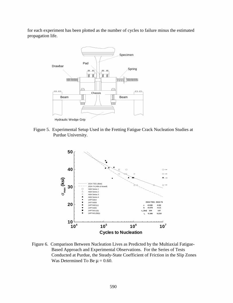
590
for each experiment has been plotted as the number of cycles to failure minus the estimatedpropagation life.
Figure 5. Experimental Setup Used in the Fretting Fatigue Crack Nucleation Studies atPurdue University.
Figure 6. Comparison Between Nucleation Lives as Predicted by the Multiaxial Fatigue-Based Approach and Experimental Observations. For the Series of TestsConducted at Purdue, the Steady-State Coefficient of Friction in the Slip ZonesWas Determined To Be µ = 0.60.
DrawbarPad
Beam Beam
Specimen
Spring
Chassis
Hydraulic Wedge Grip
104 105 106 10710
20
30
40
50
Cycles to Nucleation
σ max
(ks
i)
2024-T351 2024-T4
c -0.538 -0.52 b -0.078 -0.11
σf’ (ksi) 104 147
εf’ 0.166 0.210
2024-T351 (Blatt)
2024-T4 (Hills & Nowell)
H&N Series 1
H&N Series 2
H&N Series 3
H&N Series 4
24PTA004
24PTA008
24PTA001(c)
24PTA006
24PTA011(b)
24PTA012B(b)
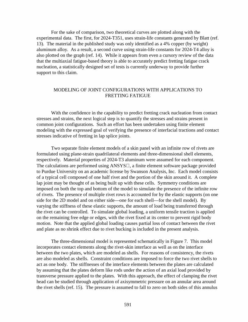
591
For the sake of comparison, two theoretical curves are plotted along with theexperimental data. The first, for 2024-T351, uses strain-life constants generated by Blatt (ref.13). The material in the published study was only identified as a 4% copper (by weight)aluminum alloy. As a result, a second curve using strain-life constants for 2024-T4 alloy isalso plotted on the graph (ref. 14). While it appears from even a cursory review of the datathat the multiaxial fatigue-based theory is able to accurately predict fretting fatigue cracknucleation, a statistically designed set of tests is currently underway to provide furthersupport to this claim.
MODELING OF JOINT CONFIGURATIONS WITH APPLICATIONS TOFRETTING FATIGUE
With the confidence in the capability to predict fretting crack nucleation from contactstresses and strains, the next logical step is to quantify the stresses and strains present incommon joint configurations. Such an effort has been undertaken using finite elementmodeling with the expressed goal of verifying the presence of interfacial tractions and contactstresses indicative of fretting in lap splice joints.
Two separate finite element models of a skin panel with an infinite row of rivets areformulated using plane-strain quadrilateral elements and three-dimensional shell elements,respectively. Material properties of 2024-T3 aluminum were assumed for each component.The calculations are performed using ANSYS, a finite element software package providedto Purdue University on an academic license by Swanson Analysis, Inc. Each model consistsof a typical cell composed of one half rivet and the portion of the skin around it. A completelap joint may be thought of as being built up with these cells. Symmetry conditions areimposed on both the top and bottom of the model to simulate the presence of the infinite rowof rivets. The presence of multiple rivet rows is accounted for by the elastic supports (on oneside for the 2D model and on either side—one for each shell—for the shell model). Byvarying the stiffness of these elastic supports, the amount of load being transferred throughthe rivet can be controlled. To simulate global loading, a uniform tensile traction is appliedon the remaining free edge or edges, with the rivet fixed at its center to prevent rigid bodymotion. Note that the applied global loading causes partial loss of contact between the rivetand plate as no shrink effect due to rivet bucking is included in the present analysis.
The three-dimensional model is represented schematically in Figure 7. This modelincorporates contact elements along the rivet-skin interface as well as on the interfacebetween the two plates, which are modeled as shells. For reasons of consistency, the rivetsare also modeled as shells. Constraint conditions are imposed to force the two rivet shells toact as one body. The stiffnesses of the interface elements between the plates are calculatedby assuming that the plates deform like rods under the action of an axial load provided bytransverse pressure applied to the plates. With this approach, the effect of clamping the rivethead can be studied through application of axisymmetric pressure on an annular area aroundthe rivet shells (ref. 15). The pressure is assumed to fall to zero on both sides of this annulus
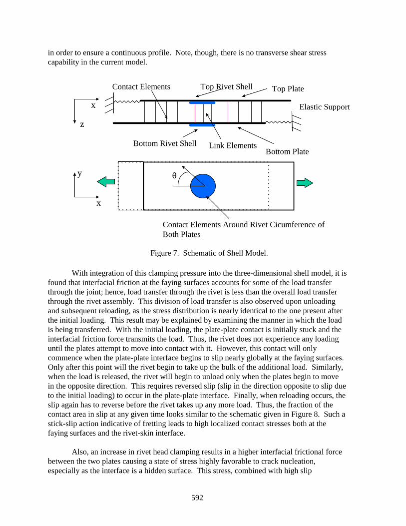
592
in order to ensure a continuous profile. Note, though, there is no transverse shear stresscapability in the current model.
Figure 7. Schematic of Shell Model.
With integration of this clamping pressure into the three-dimensional shell model, it isfound that interfacial friction at the faying surfaces accounts for some of the load transferthrough the joint; hence, load transfer through the rivet is less than the overall load transferthrough the rivet assembly. This division of load transfer is also observed upon unloadingand subsequent reloading, as the stress distribution is nearly identical to the one present afterthe initial loading. This result may be explained by examining the manner in which the loadis being transferred. With the initial loading, the plate-plate contact is initially stuck and theinterfacial friction force transmits the load. Thus, the rivet does not experience any loadinguntil the plates attempt to move into contact with it. However, this contact will onlycommence when the plate-plate interface begins to slip nearly globally at the faying surfaces.Only after this point will the rivet begin to take up the bulk of the additional load. Similarly,when the load is released, the rivet will begin to unload only when the plates begin to movein the opposite direction. This requires reversed slip (slip in the direction opposite to slip dueto the initial loading) to occur in the plate-plate interface. Finally, when reloading occurs, theslip again has to reverse before the rivet takes up any more load. Thus, the fraction of thecontact area in slip at any given time looks similar to the schematic given in Figure 8. Such astick-slip action indicative of fretting leads to high localized contact stresses both at thefaying surfaces and the rivet-skin interface.
Also, an increase in rivet head clamping results in a higher interfacial frictional forcebetween the two plates causing a state of stress highly favorable to crack nucleation,especially as the interface is a hidden surface. This stress, combined with high slip
x
x
y θ
Bottom Plate
Top PlateTop Rivet Shell
Bottom Rivet Shell Link Elements
Contact Elements
Contact Elements Around Rivet Cicumference ofBoth Plates
Elastic Support
z
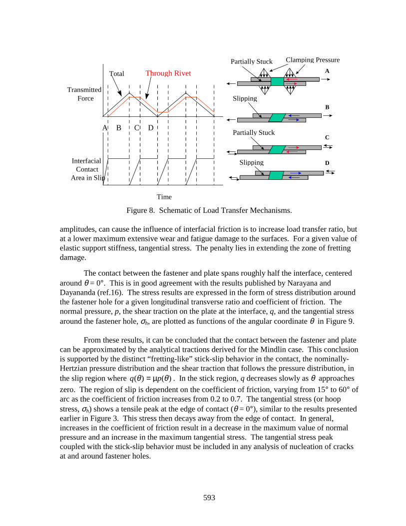
593
Figure 8. Schematic of Load Transfer Mechanisms.
amplitudes, can cause the influence of interfacial friction is to increase load transfer ratio, butat a lower maximum extensive wear and fatigue damage to the surfaces. For a given value ofelastic support stiffness, tangential stress. The penalty lies in extending the zone of frettingdamage.
The contact between the fastener and plate spans roughly half the interface, centeredaround θ = 0°. This is in good agreement with the results published by Narayana andDayananda (ref.16). The stress results are expressed in the form of stress distribution aroundthe fastener hole for a given longitudinal transverse ratio and coefficient of friction. Thenormal pressure, p, the shear traction on the plate at the interface, q, and the tangential stressaround the fastener hole, σh, are plotted as functions of the angular coordinate θ in Figure 9.
From these results, it can be concluded that the contact between the fastener and platecan be approximated by the analytical tractions derived for the Mindlin case. This conclusionis supported by the distinct “fretting-like” stick-slip behavior in the contact, the nominally-Hertzian pressure distribution and the shear traction that follows the pressure distribution, inthe slip region where q p( ) ( )θ θ= µ . In the stick region, q decreases slowly as θ approaches
zero. The region of slip is dependent on the coefficient of friction, varying from 15° to 60° ofarc as the coefficient of friction increases from 0.2 to 0.7. The tangential stress (or hoopstress, σh) shows a tensile peak at the edge of contact (θ = 0°), similar to the results presentedearlier in Figure 3. This stress then decays away from the edge of contact. In general,increases in the coefficient of friction result in a decrease in the maximum value of normalpressure and an increase in the maximum tangential stress. The tangential stress peakcoupled with the stick-slip behavior must be included in any analysis of nucleation of cracksat and around fastener holes.
Partially Stuck
B
C
Slipping
D
Partially Stuck
Slipping
A
InterfacialContact
Area in Slip
TransmittedForce
Time
Total Through Rivet
A B C D
Clamping Pressure
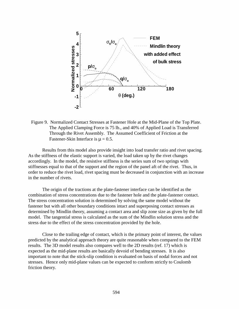
594
Figure 9. Normalized Contact Stresses at Fastener Hole at the Mid-Plane of the Top Plate.The Applied Clamping Force is 75 lb., and 40% of Applied Load is TransferredThrough the Rivet Assembly. The Assumed Coefficient of Friction at theFastener-Skin Interface is µ = 0.5.
Results from this model also provide insight into load transfer ratio and rivet spacing.As the stiffness of the elastic support is varied, the load taken up by the rivet changesaccordingly. In the model, the resistive stiffness is the series sum of two springs withstiffnesses equal to that of the support and the region of the panel aft of the rivet. Thus, inorder to reduce the rivet load, rivet spacing must be decreased in conjunction with an increasein the number of rivets.
The origin of the tractions at the plate-fastener interface can be identified as thecombination of stress concentrations due to the fastener hole and the plate-fastener contact.The stress concentration solution is determined by solving the same model without thefastener but with all other boundary conditions intact and superposing contact stresses asdetermined by Mindlin theory, assuming a contact area and slip zone size as given by the fullmodel. The tangential stress is calculated as the sum of the Mindlin solution stress and thestress due to the effect of the stress concentration provided by the hole.
Close to the trailing edge of contact, which is the primary point of interest, the valuespredicted by the analytical approach theory are quite reasonable when compared to the FEMresults. The 3D model results also compares well to the 2D results (ref. 17) which isexpected as the mid-plane results are basically devoid of bending stresses. It is alsoimportant to note that the stick-slip condition is evaluated on basis of nodal forces and notstresses. Hence only mid-plane values can be expected to conform strictly to Coulombfriction theory.
0 60 120 180
-2
-1
0
1
2
3
4
5
p/σo
FEM
θ (deg.)
No
rma
lize
d s
tre
sse
s
σh/σo
q/σo
Mindlin theory
of bulk stress
with added effect
595
As shown, the use of finite element modeling of a typical joint configuration topredict and analyze probable zones of fretting is a useful approach. It may be the only way tounderstand the behavior of the rivet-skin contact subjected to complex loadings in thepresence of cracks which may have been nucleated by fretting. This type of analysis is ofparticular significance for design of rivet size and spacing and the implications of rivetinstallation procedures in the context of widespread fatigue damage.
CONCLUSION
The combination of appropriate stresses and multiaxial fatigue theory allows theprediction of fretting crack nucleation in a two-dimensional experimental approximation ofthe rivet-skin interface. As the three-dimensional fastener-skin interfacial stress statecalculated by finite element analysis is similar to that of the experiment, it is believed that theonset of widespread fatigue damage at the fastener-skin interface can be predicted. Furtherexperimental and analytical work, particularly in the area of the stresses induced during therivet installation process, is required to predict fretting at the faying surfaces of lap joints.
REFERENCES
1. Eden, E. M; Rose, W. N.; and Cunningham, F. L.: The Endurance of Metals.Proceedings of the Institution of Mechanical Engineers, part 3, 1911, pp. 839-924.
2. Rahm, A. E. and Wurster, H. J.: Fretting Corrosion in Aircraft and AircraftAccessories. Lubrication Engineering, vol. 7, February 1951, pp. 22-40.
3. Harris, W. J.: Metallic Fatigue. Pergamon, 1961.
4. Müller, R. P. G.: An Experimental and Analytical Investigation on the FatigueBehavior of Fuselage Riveted Lap Joints. Ph.D. thesis. Delft University ofTechnology, The Netherlands, 1995.
5. Cattaneo, C.: Sul Contatto di Due Corpi Elastici: Distribuzione Locale Degli Sforze.Rendiconti dell’ Accademia nazionale dei Lincei, vol. 27, 1938, pp. 342-348, pp. 434-436, pp. 474-478.
6. Mindlin, R. D.: Compliance of Elastic Bodies in Contact. Journal of AppliedMechanics, vol. 16, 1949, pp. 259-268.
7. Szolwinski, M. P. and Farris, T. N.: Mechanics of Fretting Fatigue Crack Formation.Wear, 1996, in press.
8. McVeigh, P. A. and Farris, T. N.: Finite Element Analysis of Fretting Stresses.Journal of Tribology, 1996, in press.
596
9. Hills, D. A.; Nowell, D.; and Sackfield, A.: Surface Fatigue Considerations inFretting. Interface Dynamics, eds. Dowson, D.; Taylor, C. M.; Godet, M.; andBerthe, D., Elsevier, 1988, pp. 35-40.
10. Hills, D. A.; Nowell, D.; and O’Connor, J. J.: On the Mechanics of Fretting Fatigue.Wear, 1988, vol. 125, pp. 129-156.
11. Socie, D.: Critical Plane Approaches for Multiaxial Fatigue Damage Assessment.Advances in Multiaxial Fatigue, ASTM STP 1191, 1993, pp. 7-36.
12. Szolwinski, M. P.; Harish, G.; and Farris, T. N.: Experimental Observation of theEffect of Contact Parameters on Fretting Fatigue Crack Nucleation. Proceedings ofthe 1995 USAF Structural Integrity Program Conference, San Antonio, 1995.
13. Blatt, P. A.: Evaluation of Fatigue Crack Initiation Behavior of an ExperimentalTernary Aluminum-Lithium Alloy. M. S. thesis, Purdue University, West Lafayette,1990.
14. Hertzberg, R. W.: Deformation and Fracture Mechanics of Engineering Materials.Wiley, 1976.
15. Reithmaier, L.: Standard Aircraft Handbook. 4th ed., Tab Books, 1986.
16. Narayana, K. B. and Dayananda, T. S.: Cracks Emanating from Pin-Loaded Joints.Egg. Fracture Mechanics, vol. 47, 1994, pp. 29-38.
17. Farris, T. N.; Grandt, A. F., Jr.; Harish, G.; and Wang, H. L.: Analysis of WidespreadFatigue Damage in Structural Joints. Proceedings of 41st International SAMPESymposium and Exhibition, Anaheim, 1996.
597
THE ROLE OF NEW-TECHNOLOGYNONDESTRUCTIVE INSPECTION TECHNIQUES
A. Quincy HowardBoeing Commercial Airplane Group
Seattle, WA 98124
SUMMARY
There has been a large nondestructive inspection (NDI) research and developmenteffort directed toward the use of new technology. Many of the techniques developed arewide-area techniques designed to help decrease the time and human factor difficultiesinvolved with existing techniques. Although many of the existing service bulletin (SB)inspections may not benefit by these new-technology techniques, the increased use ofadvanced composite materials provides an excellent opportunity for these techniques to beutilized. This paper describes where these new-technology techniques might be used, both inexisting and future applications.
INTRODUCTION
Commercial airplanes are designed to be damage tolerant, that is, able to sustainregulatory loads in the presence of damage until the damage is detected through inspection ormalfunction and repaired. Corrosion and fatigue are such types of damage that can occur toan airplane. It is the goal of an Original Equipment Manufacturer (OEM) to design airplanesto be resistant to corrosion and fatigue and to develop maintenance programs that provideopportunities to identify damage before the airplane’s residual strength is impaired.
This residual strength requirement is one of the primary concerns in selecting aninspection method. The goal of inspection is not necessarily to ensure that there is absolutelyno damage, but to ensure that the residual strength of the structural member is notcompromised.
LAP JOINT INSPECTIONS
The inspection requirements for the B727, B737, and B747 model lap joints havebeen the focus of much attention. Service Bulletin 737-53A1039 addresses the longitudinallap joints of the B737. The requirements of this service bulletin are similar to those for theB727 and B747 airplanes. In this service bulletin, visual inspection is the method used toidentify the presence of corrosion. The service bulletin requires that if there are visual signs
598
of corrosion, these areas must be inspected with low-frequency eddy current to determine theamount of material loss. (The B727 equivalent service bulletin requires the entire skin panelbe inspected for material loss.) Eddy-current inspection is the current NDI method of choicebecause the equipment is relatively inexpensive and portable, and the method is able toestimate material loss.
Many new-technology NDI techniques have been investigated for the lap jointdisbond/corrosion problem. Since there is such a large amount of lap splice area, theseservice bulletins appear to be good candidates for these techniques. Many of thesetechniques are able to detect the presence of disbonding or corrosion, but at this time, theyare unable to quantify the amount of material loss. If these methods were to be usedcurrently, they would only be replacing a visual inspection, as the eddy-current inspectionwould still be required to estimate the amount of remaining material.
It is also important to note that the lap joint corrosion problem is applicable to alimited number of airplanes. The service bulletin requirements for corrosion inspections areonly applicable to line numbers 1 to 849 for the B727, 1 to 291 for the B737, and l to 200 forthe B747. After these line numbers, the lap joints, as well as all airplanes built thereafter,were assembled with sealant between the skin panels. This lap joint configuration has notexperienced a corrosion problem. The number of applicable airplanes is becoming smaller assome airplanes are modified and others retired due to age.
NDI FOR CORROSION
Corrosion problems occur in more areas than just lap joints. Because of theincreasing problem with corrosion as airplanes age, the Corrosion Prevention and ControlProgram (CPCP) was developed by industry. The CPCP is mandated by the FAA for allmodel airplanes, and it requires operators to perform repeat visual inspections on all airplanestructure at designated intervals. The fact that all airplane models are affected and that largeareas of each airplane are inspected would lead some to believe that new-technologyinspection techniques could be a big help to CPCP inspections. One must look at theprogram as a whole, however, to see why visual inspection was chosen.
There are several different parts to CPCP implementation. Along with the visualinspection task are tasks of reapplying any damaged protective finishes, clearing drain paths,applying corrosion inhibiting compounds, and drying insulation blankets. All of these stepsmust be performed even if there is no corrosion found, and therefore, internal access must begained. Since access must be gained, it makes sense to perform a visual inspection ratherthan use a new-technology inspection technique.
Many service bulletins allow the option of external inspection using an NDItechnique or internal visual inspection. The existence of the CPCP may influence whichinspection option an operator chooses. For instance, if a service bulletin inspection is to becarried out, a visual inspection can be performed during the CPCP inspection with no
599
additional time for gaining access, and many times, with no additional time for inspection(i.e., the same area is being looked at with the same level of inspection). If an operator has achoice of a visual inspection with an interval equal to or greater than the CPCP interval or anexternal NDI technique, it might make sense to perform the visual inspection, since accesswill already have been gained for the CPCP inspection.
Visual inspection, however, is not always the best inspection method for corrosiondetection. Recent advances in the use of ultrasonics to detect and measure corrosion insecond-layer structure has made this new-technology technique very useful. Although not awide-area technique, it has been shown to save many hours over existing visual inspections[1]. The use of this technique does require that the structure being inspected be sealed at thefaying surfaces.
Other advanced technology techniques, such as D-sight [2], infrared thermography[3], and Magneto-Optic Imaging [4], are able to find areas of corrosion. At this time,however, they are unable to estimate the amount of material loss. These techniques may stillbe useful to supplement visual inspections for detecting hidden corrosion.
SERVICE BULLETIN INSPECTIONS
Much of the NDI research and development effort has been directed toward servicebulletin applications, such as lap joint inspections. Much of the research has been directedtoward so-called wide-area techniques to help decrease the time and human factorsdifficulties involved in these inspections. A study was done recently to identify how manyBoeing service bulletins could be applicable to wide-area techniques for corrosion anddisbond detection. The selection of these service bulletins did not mean that a wide-areatechnique should be used or was necessarily beneficial, only that it was possible that onecould be used.
Six B727, six B737, and four B747 service bulletins were selected as candidates forpossible wide-area inspection applications. These numbers are reduced if the wide-areatechnique cannot measure the amount of material loss caused by corrosion. As discussedpreviously, if the technique is not capable of doing this, it simply replaces an external visualinspection and may not be of any benefit.
Table 1 shows the B727 service bulletins selected, the current inspection method, andthe amount of time estimated to accomplish the inspection. No time estimates are given forthe eddy-current inspections for corrosion, because the amount of time depends on the arearequiring inspection and how much corrosion is present. Again, the listing of these bulletinsdoes not mean that a wide-area technique would be beneficial, but rather that a wide-areatechnique could be of possible benefit.
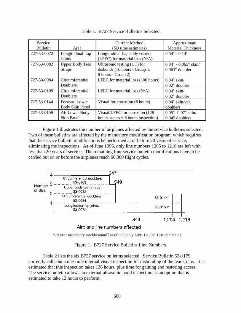
600
Table 1. B727 Service Bulletins Selected.
ServiceBulletin Area
Current Method(SB time estimates)
ApproximateMaterial Thickness
727-53-0072 Longitudinal LapJoints
Longitudinal flap eddy current(LFEC) for material loss (N/A)
0.04″ - 0.14″
727-53-0082 Upper Body TearStraps
Ultrasonic testing (UT) fordisbonds (16 hours - Group 1,8 hours - Group 2)
0.04″ - 0.065″ skin/0.063″ doubler
727-53-0084 CircumferentialDoublers
LFEC for material loss (100 hours) 0.04″ skin/0.02″ doubler
727-53-0109 CircumferentialDoublers
LFEC for material loss (N/A) 0.04″ skin/0.02″ doubler
727-53-0144 Forward LowerBody Skin Panel
Visual for corrosion (8 hours) 0.04″ skin/var.doublers
727-53-0159 Aft Lower BodySkin Panel
Visual/LFEC for corrosion (128hours access + 8 hours inspection)
0.05″ -0.07″ skin/0.045 doublers
Figure 1 illustrates the number of airplanes affected by the service bulletins selected.Two of these bulletins are affected by the mandatory modification program, which requiresthat the service bulletin modifications be performed at or before 20 years of service,eliminating the inspections. As of June 1996, only line numbers 1205 to 1216 are left withless than 20 years of service. The remaining four service bulletin modifications have to becarried out on or before the airplanes reach 60,000 flight cycles.
*20-year mandatory modificationas of 6/96 only L/Ns 1205 to 1216 remaining
Figure 1. B727 Service Bulletins Line Numbers.
Table 2 lists the six B737 service bulletins selected. Service Bulletin 53-1179currently calls out a one-time internal visual inspection for disbonding of the tear straps. It isestimated that this inspection takes 136 hours, plus time for gaining and restoring access.The service bulletin allows an external ultrasonic bond inspection as an option that isestimated to take 12 hours to perform.
Numberof SBs
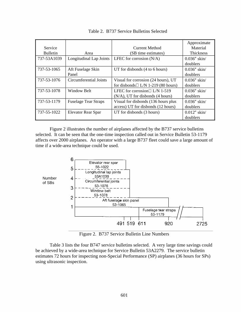
601
Table 2. B737 Service Bulletins Selected
ServiceBulletin Area
Current Method(SB time estimates)
ApproximateMaterial
Thickness737-53A1039 Longitudinal Lap Joints LFEC for corrosion (N/A) 0.036″ skin/
doublers737-53-1065 Aft Fuselage Skin
PanelUT for disbonds (4 to 6 hours) 0.036″ skin/
doublers737-53-1076 Circumferential Joints Visual for corrosion (24 hours), UT
for disbondsL/N 1-219 (80 hours)0.036″ skin/doublers
737-53-1078 Window Belt LFEC for corrosionL/N 1-519(N/A), UT for disbonds (4 hours)
0.036″ skin/doublers
737-53-1179 Fuselage Tear Straps Visual for disbonds (136 hours plusaccess) UT for disbonds (12 hours)
0.036″ skin/doublers
737-55-1022 Elevator Rear Spar UT for disbonds (3 hours) 0.012″ skin/doublers
Figure 2 illustrates the number of airplanes affected by the B737 service bulletinsselected. It can be seen that the one-time inspection called out in Service Bulletin 53-1179affects over 2000 airplanes. An operator with a large B737 fleet could save a large amount oftime if a wide-area technique could be used.
Figure 2. B737 Service Bulletin Line Numbers
Table 3 lists the four B747 service bulletins selected. A very large time savings couldbe achieved by a wide-area technique for Service Bulletin 53A2279. The service bulletinestimates 72 hours for inspecting non-Special Performance (SP) airplanes (36 hours for SPs)using ultrasonic inspection.
Numberof SBs
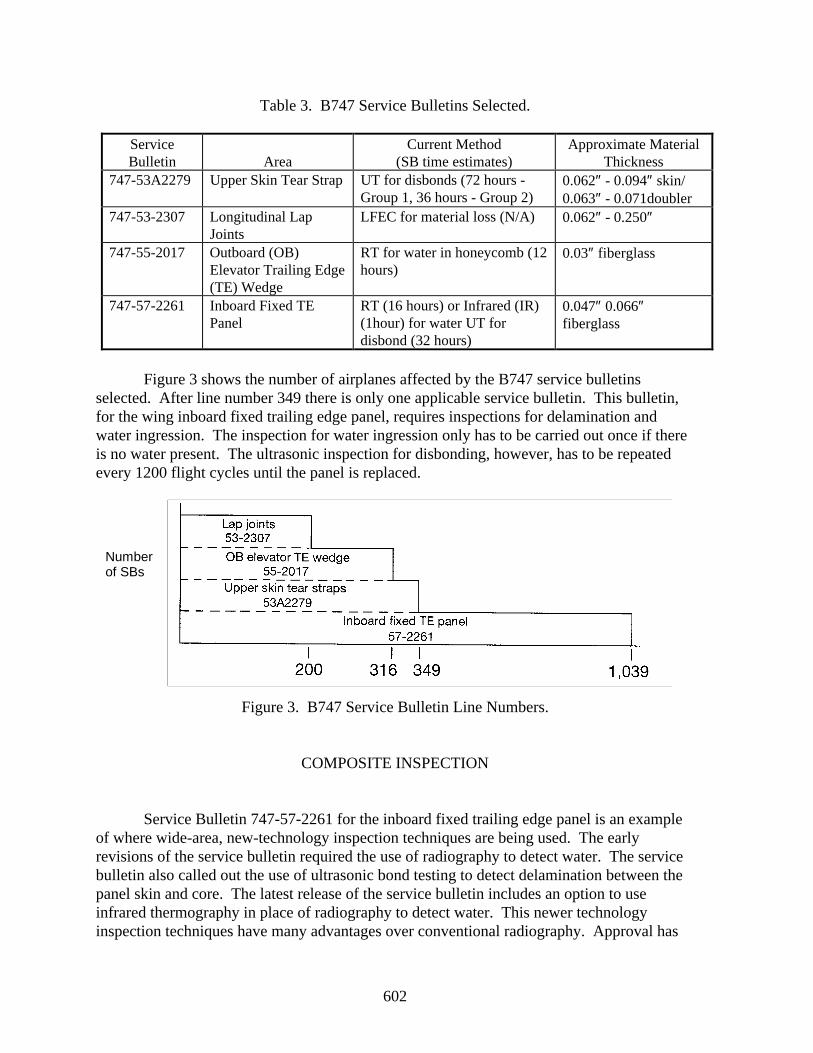
602
Table 3. B747 Service Bulletins Selected.
ServiceBulletin Area
Current Method(SB time estimates)
Approximate MaterialThickness
747-53A2279 Upper Skin Tear Strap UT for disbonds (72 hours -Group 1, 36 hours - Group 2)
0.062″ - 0.094″ skin/0.063″ - 0.071doubler
747-53-2307 Longitudinal LapJoints
LFEC for material loss (N/A) 0.062″ - 0.250″
747-55-2017 Outboard (OB)Elevator Trailing Edge(TE) Wedge
RT for water in honeycomb (12hours)
0.03″ fiberglass
747-57-2261 Inboard Fixed TEPanel
RT (16 hours) or Infrared (IR)(1hour) for water UT fordisbond (32 hours)
0.047″ 0.066″fiberglass
Figure 3 shows the number of airplanes affected by the B747 service bulletinsselected. After line number 349 there is only one applicable service bulletin. This bulletin,for the wing inboard fixed trailing edge panel, requires inspections for delamination andwater ingression. The inspection for water ingression only has to be carried out once if thereis no water present. The ultrasonic inspection for disbonding, however, has to be repeatedevery 1200 flight cycles until the panel is replaced.
Figure 3. B747 Service Bulletin Line Numbers.
COMPOSITE INSPECTION
Service Bulletin 747-57-2261 for the inboard fixed trailing edge panel is an exampleof where wide-area, new-technology inspection techniques are being used. The earlyrevisions of the service bulletin required the use of radiography to detect water. The servicebulletin also called out the use of ultrasonic bond testing to detect delamination between thepanel skin and core. The latest release of the service bulletin includes an option to useinfrared thermography in place of radiography to detect water. This newer technologyinspection techniques have many advantages over conventional radiography. Approval has
Numberof SBs
603
also been given for the use of laser shearography in place of the bond test procedure calledout in the service bulletin. This service bulletin is a good example of the great potential fornew-technology inspection techniques.
The increased use of advanced composite materials provides a great opportunity fornew-technology NDI techniques to be used. The introduction of the B737-300, B757, andB767 airplanes in the 1980s created a demand for new NDI techniques to inspect theadvanced composite materials. Although there are a few composite parts, such as the B757and B767 rudder and elevators, that require ultrasonic inspection for delamination, theprimary inspection method is visual for evidence of damage, such as damage from impact orlightening strike. NDI techniques are then used to assess the damage and inspect the ensuingrepair. Damage assessment is usually performed with a tap test or ultrasonic inspection, andit is relatively straightforward. The use of ultrasonics for composite repair inspection,however, has proven to be difficult, and some of the new-technology techniques may offeradvantages, such as simplified interpretation of results.
Although existing techniques are currently meeting the needs of compositeinspection, there is a potential for improvements with new-technology techniques. Already,infrared thermography has been shown to be an excellent replacement for radiographicdetection of water and ice in honeycomb. Thermography has been shown to save time, withequivalent results, without the radiation hazard [5]. The need for advanced inspectiontechniques will also increase as airplanes like the B777, with composite primary structure,grow older.
CONCLUSIONS
New-technology inspection techniques offer a big potential in the airplane industry.It is important, however, that the techniques fit into the overall picture of damage tolerance.In some cases, the technique that can find the smallest defect may not be the technique ofchoice.
The detection of hidden corrosion is a concern on older model airplanes. Visualinspection has been used as the primary means of detecting hidden corrosion in such areas aslap joints. Visual inpsection is also the method used in the FAA-mandated CorrosionPrevention and Control Program for all model airplanes. For almost all Boeing commercialairplane applications, visual inspection for corrosion is more than adequate to meet theinspection requirements.
A detailed study of existing service bulletins for the B727, B737, and B747 showedthat there are some applications for wide-area, new-technology techniques. Many of thesepotential applications require that the new techniques be able to estimate the amount ofcorrosion material loss before it can effectively replace the existing eddy-current technique.There is a possible large time savings for one B737 and one B747 service bulletin currentlycalling out ultrasonic bond inspection.
604
The expanded use of advanced composite materials provides the greatest opportunityto maximize the benefit from new-technology techniques. Although existing methods arecapable of performing these inspections, research and development into newer and moreadvanced techniques is an important part of improving the overall inspection process.
The Boeing Company will continue to research new-technology techniques and try toidentify new applications. We will also continue to monitor the research into thesetechniques being done throughout the industry, and we will encourage the advancement ofNDI technology.
REFERENCES
1. Komsky, I. N. et al.: An Ultrasonic Technique to Detect Corrosion in DC-9 WingBox From Concept to Field Application, Materials Evaluation, Vol. 53, No. 7,July 1995, pp. 848-852.
2. Komorowski, J. P. et al.: Double Pass Retroreflection for Corrosion Detection inAircraft Structures, Materials Evaluation, Vol. 54, No. 1, January 1996, pp. 80-86.
3. Favro, L. D. et al.: Thermal Wave Imaging of Aircraft Structures, Review of Progressin Quantitative NDE, Vol. 14, pp. 461-466, Edited by D. O. Thompson and D. E.Chimenti, Plenum Press, New York, 1995.
4. Fitzpatrick, G. I. et al.: Magneto-Optic/Eddy-Current Imaging of SubsurfaceCorrosion and Fatigue Cracks in Aging Aircraft, Review of Progress in QuantitativeNDE, Vol. 15, pp. 1159-1166, Edited by D. O. Thompson and D. E. Chimenti,Plenum Press, New York, 1996.
5. Thompson, J. G.: Thermography for Honeycomb Panel Inspection, Review ofProgress in Quantitative Nondestructive Evaluation, Vol. 15B, Plenum Press,New York, 1996, pp. 1271-1274.
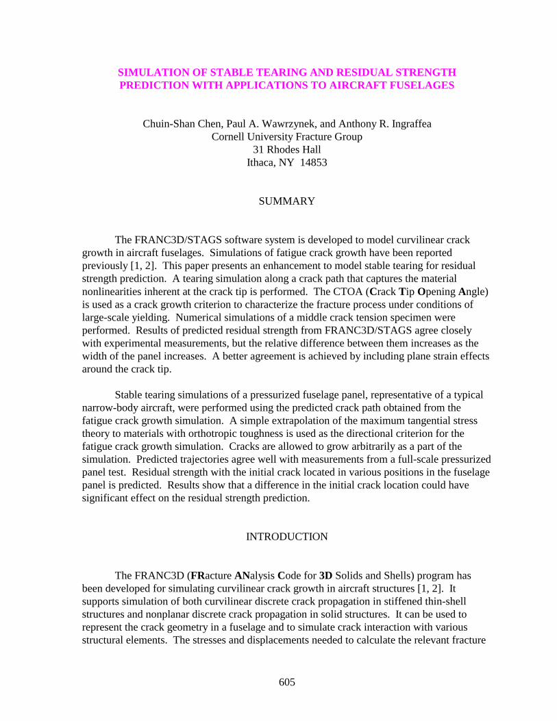
605
SIMULATION O F STABLE TEARING AND RESIDUAL STRENGTHPREDICTION WITH A PPLICATIONS TO AIRCRA FT FUSELAGES
Chuin-Shan Chen, Paul A. Wawrzynek, and Anthony R. IngraffeaCornell University Fracture Group
31 Rhodes HallIthaca, NY 14853
SUMMARY
The FRANC3D/STAGS software system is developed to model curvilinear crackgrowth in aircraft fuselages. Simulations of fatigue crack growth have been reportedpreviously [1, 2]. This paper presents an enhancement to model stable tearing for residualstrength prediction. A tearing simulation along a crack path that captures the materialnonlinearities inherent at the crack tip is performed. The CTOA (Crack Tip Opening Angle)is used as a crack growth criterion to characterize the fracture process under conditions oflarge-scale yielding. Numerical simulations of a middle crack tension specimen wereperformed. Results of predicted residual strength from FRANC3D/STAGS agree closelywith experimental measurements, but the relative difference between them increases as thewidth of the panel increases. A better agreement is achieved by including plane strain effectsaround the crack tip.
Stable tearing simulations of a pressurized fuselage panel, representative of a typicalnarrow-body aircraft, were performed using the predicted crack path obtained from thefatigue crack growth simulation. A simple extrapolation of the maximum tangential stresstheory to materials with orthotropic toughness is used as the directional criterion for thefatigue crack growth simulation. Cracks are allowed to grow arbitrarily as a part of thesimulation. Predicted trajectories agree well with measurements from a full-scale pressurizedpanel test. Residual strength with the initial crack located in various positions in the fuselagepanel is predicted. Results show that a difference in the initial crack location could havesignificant effect on the residual strength prediction.
INTRODUCTION
The FRANC3D (FRacture ANalysis Code for 3D Solids and Shells) program hasbeen developed for simulating curvilinear crack growth in aircraft structures [1, 2]. Itsupports simulation of both curvilinear discrete crack propagation in stiffened thin-shellstructures and nonplanar discrete crack propagation in solid structures. It can be used torepresent the crack geometry in a fuselage and to simulate crack interaction with variousstructural elements. The stresses and displacements needed to calculate the relevant fracture
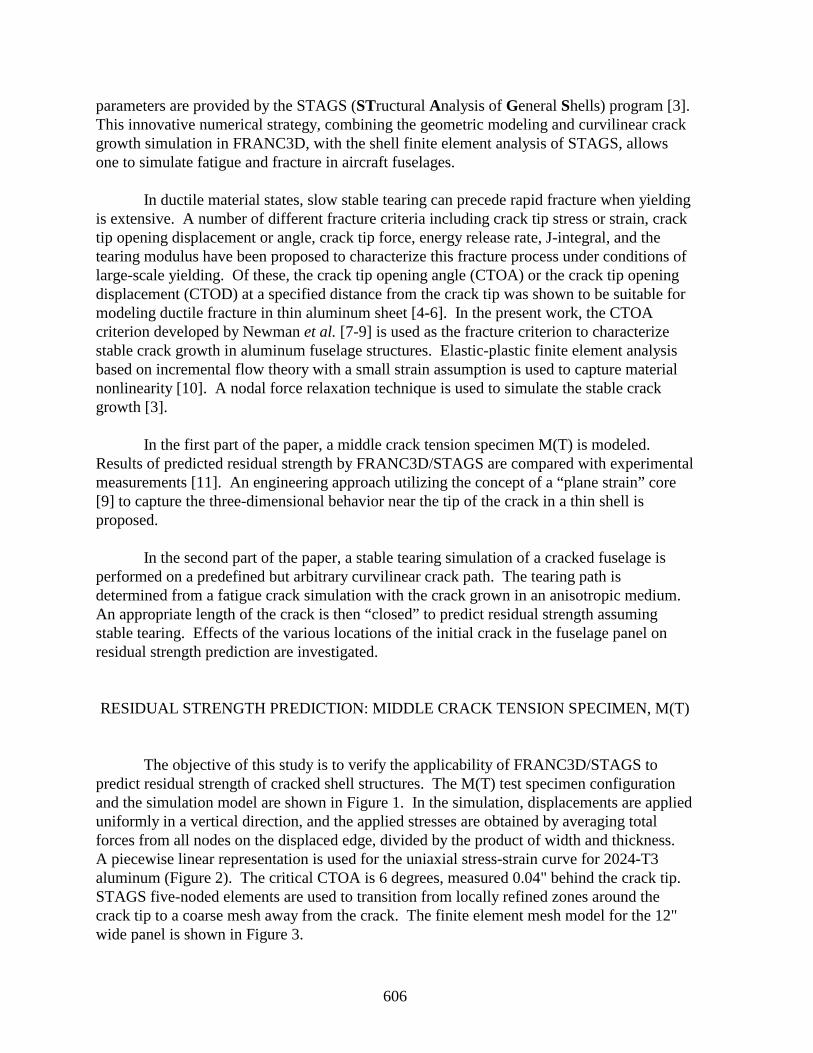
606
parameters are provided by the STAGS (STructural Analysis of General Shells) program [3].This innovative numerical strategy, combining the geometric modeling and curvilinear crackgrowth simulation in FRANC3D, with the shell finite element analysis of STAGS, allowsone to simulate fatigue and fracture in aircraft fuselages.
In ductile material states, slow stable tearing can precede rapid fracture when yieldingis extensive. A number of different fracture criteria including crack tip stress or strain, cracktip opening displacement or angle, crack tip force, energy release rate, J-integral, and thetearing modulus have been proposed to characterize this fracture process under conditions oflarge-scale yielding. Of these, the crack tip opening angle (CTOA) or the crack tip openingdisplacement (CTOD) at a specified distance from the crack tip was shown to be suitable formodeling ductile fracture in thin aluminum sheet [4-6]. In the present work, the CTOAcriterion developed by Newman et al. [7-9] is used as the fracture criterion to characterizestable crack growth in aluminum fuselage structures. Elastic-plastic finite element analysisbased on incremental flow theory with a small strain assumption is used to capture materialnonlinearity [10]. A nodal force relaxation technique is used to simulate the stable crackgrowth [3].
In the first part of the paper, a middle crack tension specimen M(T) is modeled.Results of predicted residual strength by FRANC3D/STAGS are compared with experimentalmeasurements [11]. An engineering approach utilizing the concept of a “plane strain” core[9] to capture the three-dimensional behavior near the tip of the crack in a thin shell isproposed.
In the second part of the paper, a stable tearing simulation of a cracked fuselage isperformed on a predefined but arbitrary curvilinear crack path. The tearing path isdetermined from a fatigue crack simulation with the crack grown in an anisotropic medium.An appropriate length of the crack is then “closed” to predict residual strength assumingstable tearing. Effects of the various locations of the initial crack in the fuselage panel onresidual strength prediction are investigated.
RESIDUAL STRENGTH PREDICTION: MIDDLE CRACK TENSION SPECIMEN, M(T)
The objective of this study is to verify the applicability of FRANC3D/STAGS topredict residual strength of cracked shell structures. The M(T) test specimen configurationand the simulation model are shown in Figure 1. In the simulation, displacements are applieduniformly in a vertical direction, and the applied stresses are obtained by averaging totalforces from all nodes on the displaced edge, divided by the product of width and thickness.A piecewise linear representation is used for the uniaxial stress-strain curve for 2024-T3aluminum (Figure 2). The critical CTOA is 6 degrees, measured 0.04" behind the crack tip.STAGS five-noded elements are used to transition from locally refined zones around thecrack tip to a coarse mesh away from the crack. The finite element mesh model for the 12"wide panel is shown in Figure 3.
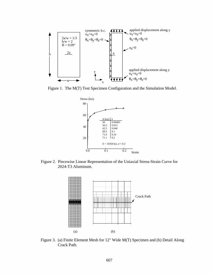
607
w
h 2a
2a/w = 1/3h/w = 2B = 0.09"
symmetric b.c.ux=uz=0
θx=θy=θz=0
uz=0
applied displacement along yux=uz=0
θx=θy=θz=0
applied displacement along yux=uz=0
θx=θy=θz=0
x
y
a
Figure 1. The M(T) Test Specimen Configuration and the Simulation Model.
Stress (ksi)
Strain0.0 0.1 0.2
20
40
60
80
σ (ksi) ε50 0.0048356.5 0.01562.5 0.04068.5 0.171.0 0.1671.1 0.2
E = 10350 ksi, ν = 0.3
Figure 2. Piecewise Linear Representation of the Uniaxial Stress-Strain Curve for2024-T3 Aluminum.
crack path
(a) (b)
Figure 3. (a) Finite Element Mesh for 12" Wide M(T) Specimen and (b) Detail AlongCrack Path.
(a) (b)
Crack Path
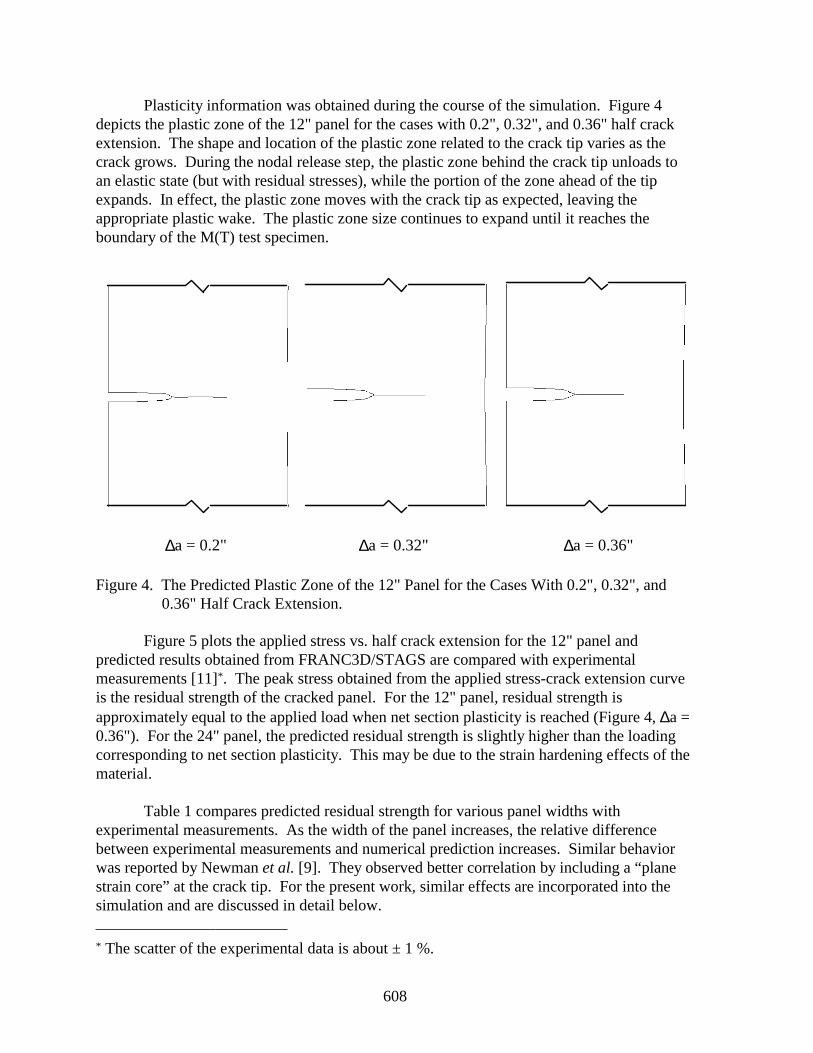
608
Plasticity information was obtained during the course of the simulation. Figure 4depicts the plastic zone of the 12" panel for the cases with 0.2", 0.32", and 0.36" half crackextension. The shape and location of the plastic zone related to the crack tip varies as thecrack grows. During the nodal release step, the plastic zone behind the crack tip unloads toan elastic state (but with residual stresses), while the portion of the zone ahead of the tipexpands. In effect, the plastic zone moves with the crack tip as expected, leaving theappropriate plastic wake. The plastic zone size continues to expand until it reaches theboundary of the M(T) test specimen.
∆a = 0.2" ∆a = 0.32" ∆a = 0.36"
Figure 4. The Predicted Plastic Zone of the 12" Panel for the Cases With 0.2", 0.32", and0.36" Half Crack Extension.
Figure 5 plots the applied stress vs. half crack extension for the 12" panel andpredicted results obtained from FRANC3D/STAGS are compared with experimentalmeasurements [11]*. The peak stress obtained from the applied stress-crack extension curveis the residual strength of the cracked panel. For the 12" panel, residual strength isapproximately equal to the applied load when net section plasticity is reached (Figure 4, ∆a =0.36"). For the 24" panel, the predicted residual strength is slightly higher than the loadingcorresponding to net section plasticity. This may be due to the strain hardening effects of thematerial.
Table 1 compares predicted residual strength for various panel widths withexperimental measurements. As the width of the panel increases, the relative differencebetween experimental measurements and numerical prediction increases. Similar behaviorwas reported by Newman et al. [9]. They observed better correlation by including a “planestrain core” at the crack tip. For the present work, similar effects are incorporated into thesimulation and are discussed in detail below.
* The scatter of the experimental data is about ± 1 %.
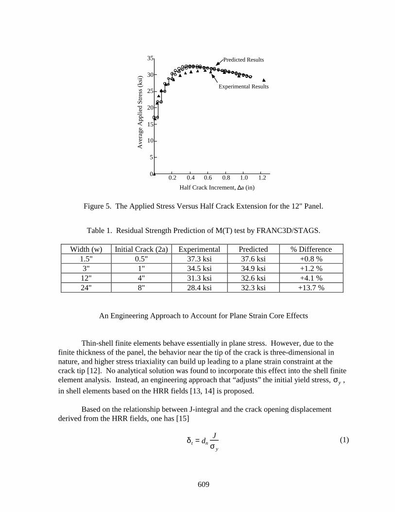
609
.
0.2 0.4 0.6 0.8 1.0 1.20
5
10
15
20
25
30
35
Half Crack Increment, ∆a (in)
Ave
rag
e A
pp
lied
Str
ess
(ks
i)
predicted results
experimental results
Figure 5. The Applied Stress Versus Half Crack Extension for the 12" Panel.
Table 1. Residual Strength Prediction of M(T) test by FRANC3D/STAGS.
Width (w) Initial Crack (2a) Experimental Predicted % Difference1.5" 0.5" 37.3 ksi 37.6 ksi +0.8 %3" 1" 34.5 ksi 34.9 ksi +1.2 %12" 4" 31.3 ksi 32.6 ksi +4.1 %24" 8" 28.4 ksi 32.3 ksi +13.7 %
An Engineering Approach to Account for Plane Strain Core Effects
Thin-shell finite elements behave essentially in plane stress. However, due to thefinite thickness of the panel, the behavior near the tip of the crack is three-dimensional innature, and higher stress triaxiality can build up leading to a plane strain constraint at thecrack tip [12]. No analytical solution was found to incorporate this effect into the shell finiteelement analysis. Instead, an engineering approach that “adjusts” the initial yield stress, σy ,
in shell elements based on the HRR fields [13, 14] is proposed.
Based on the relationship between J-integral and the crack opening displacementderived from the HRR fields, one has [15]
δ t = dnJ
σ y
(1)
Experimental Results
Predicted Results
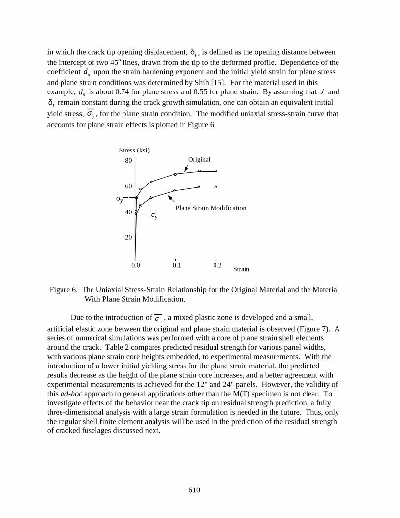
610
in which the crack tip opening displacement, δ t , is defined as the opening distance betweenthe intercept of two 45o lines, drawn from the tip to the deformed profile. Dependence of thecoefficient dn upon the strain hardening exponent and the initial yield strain for plane stressand plane strain conditions was determined by Shih [15]. For the material used in thisexample, dn is about 0.74 for plane stress and 0.55 for plane strain. By assuming that J andδ t remain constant during the crack growth simulation, one can obtain an equivalent initial
yield stress, σ y , for the plane strain condition. The modified uniaxial stress-strain curve that
accounts for plane strain effects is plotted in Figure 6.
Stress (ksi)
Strain
Plane Strain Modification
original
0.0 0.1 0.2
20
40
60
80
σy
σy
Figure 6. The Uniaxial Stress-Strain Relationship for the Original Material and the Material With Plane Strain Modification.
Due to the introduction of σ y, a mixed plastic zone is developed and a small,
artificial elastic zone between the original and plane strain material is observed (Figure 7). Aseries of numerical simulations was performed with a core of plane strain shell elementsaround the crack. Table 2 compares predicted residual strength for various panel widths,with various plane strain core heights embedded, to experimental measurements. With theintroduction of a lower initial yielding stress for the plane strain material, the predictedresults decrease as the height of the plane strain core increases, and a better agreement withexperimental measurements is achieved for the 12" and 24" panels. However, the validity ofthis ad-hoc approach to general applications other than the M(T) specimen is not clear. Toinvestigate effects of the behavior near the crack tip on residual strength prediction, a fullythree-dimensional analysis with a large strain formulation is needed in the future. Thus, onlythe regular shell finite element analysis will be used in the prediction of the residual strengthof cracked fuselages discussed next.
Original
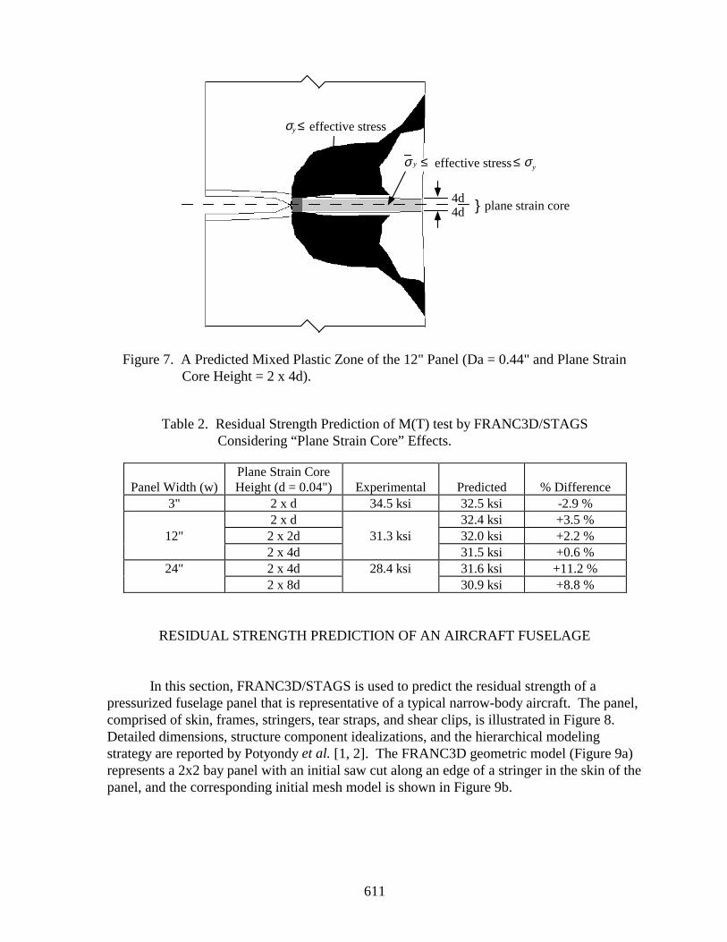
611
σy ≤ effective stress
plane strain core
σ y ≤ effective stress≤ σy
4d4d
Figure 7. A Predicted Mixed Plastic Zone of the 12" Panel (Da = 0.44" and Plane StrainCore Height = 2 x 4d).
Table 2. Residual Strength Prediction of M(T) test by FRANC3D/STAGS Considering “Plane Strain Core” Effects.
Panel Width (w)Plane Strain CoreHeight (d = 0.04") Experimental Predicted % Difference
3" 2 x d 34.5 ksi 32.5 ksi -2.9 %2 x d 32.4 ksi +3.5 %
12" 2 x 2d 31.3 ksi 32.0 ksi +2.2 %2 x 4d 31.5 ksi +0.6 %
24" 2 x 4d 28.4 ksi 31.6 ksi +11.2 %2 x 8d 30.9 ksi +8.8 %
RESIDUAL STRENGTH PREDICTION OF AN AIRCRAFT FUSELAGE
In this section, FRANC3D/STAGS is used to predict the residual strength of apressurized fuselage panel that is representative of a typical narrow-body aircraft. The panel,comprised of skin, frames, stringers, tear straps, and shear clips, is illustrated in Figure 8.Detailed dimensions, structure component idealizations, and the hierarchical modelingstrategy are reported by Potyondy et al. [1, 2]. The FRANC3D geometric model (Figure 9a)represents a 2x2 bay panel with an initial saw cut along an edge of a stringer in the skin of thepanel, and the corresponding initial mesh model is shown in Figure 9b.

612
stringer
skin• fuselage radius =74"
frame
tear straps• under stringers• under frames• at midbay
shear clip
Figure 8. The Structural Components of a Typical Narrow-Body Aircraft Fuselage.
crack
Figure 9. (a) The FRANC3D Geometric Model, and (b) the Mesh Model With an InitialCrack Along an Edge of a Stringer in the Skin of the Panel.
A geometrically nonlinear elastic analysis of fatigue crack growth is performed first.An appropriate length of crack is then “closed” to perform a tearing simulation that includesboth geometric and material nonlinear effects. The possible trajectory change due to stabletearing is neglected, and the transition from fatigue to tearing is assumed to occur abruptlyand the plasticity history prior to tearing is ignored for this analysis.
Crack Trajectory Prediction
Crack trajectories are predicted based on fatigue crack growth simulation. A set offour stress intensity factors (k1, k2, KI, KII ) proposed by Hui and Zehnder [16] accounts forboth the in-plane membrane loading (KI, KII ) and the out-of-plane bending loading (k1, k2)experienced by a crack in a fuselage structure. For each crack growth simulation cycle, theequilibrium state with fully applied loading is obtained from a geometrically nonlinear shellanalysis. Stress intensity factors are computed using the modified crack closure integralmethod [17].
(a) (b)
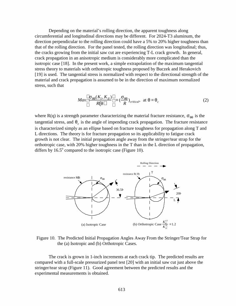
613
Depending on the material’s rolling direction, the apparent toughness alongcircumferential and longitudinal directions may be different. For 2024-T3 aluminum, thedirection perpendicular to the rolling direction could have a 5% to 20% higher toughness thanthat of the rolling direction. For the panel tested, the rolling direction was longitudinal; thus,the cracks growing from the initial saw cut are experiencing T-L crack growth. In general,crack propagation in an anisotropic medium is considerably more complicated than theisotropic case [18]. In the present work, a simple extrapolation of the maximum tangentialstress theory to materials with orthotropic toughness proposed by Buczek and Herakovich[19] is used. The tangential stress is normalized with respect to the directional strength of thematerial and crack propagation is assumed to be in the direction of maximum normalizedstress, such that
Maxσθθ(KI ,KII )
R θ( )
= (σθθ
R)critical, at θ = θc (2)
where R(q) is a strength parameter characterizing the material fracture resistance, σθθ is thetangential stress, and θc is the angle of impending crack propagation. The fracture resistanceis characterized simply as an ellipse based on fracture toughness for propagation along T andL directions. The theory is for fracture propagation so its applicability to fatigue crackgrowth is not clear. The initial propagation angle away from the stringer/tear strap for theorthotropic case, with 20% higher toughness in the T than in the L direction of propagation,differs by 16.5o compared to the isotropic case (Figure 10).
35.15°36.5Þ
L
Tresistance R(θ)
σθθresistance R(θ) σθθ
Rolling Direction
20°
(a) Isotropic Case (b) Orthotropic CaseKIC
LT
KICTL =1.2
20Þ
Figure 10. The Predicted Initial Propagation Angles Away From the Stringer/Tear Strap forthe (a) Isotropic and (b) Orthotropic Cases.
The crack is grown in 1-inch increments at each crack tip. The predicted results arecompared with a full-scale pressurized panel test [20] with an initial saw cut just above thestringer/tear strap (Figure 11). Good agreement between the predicted results and theexperimental measurements is obtained.
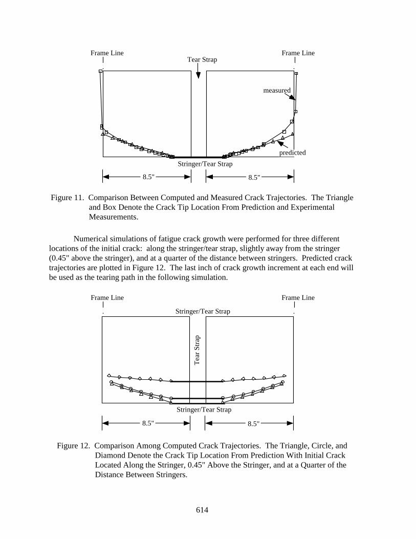
614
8.5" 8.5"
predicted
measured
Frame LineTear Strap
Stringer/Tear Strap
Frame Line
Figure 11. Comparison Between Computed and Measured Crack Trajectories. The Triangleand Box Denote the Crack Tip Location From Prediction and ExperimentalMeasurements.
Numerical simulations of fatigue crack growth were performed for three differentlocations of the initial crack: along the stringer/tear strap, slightly away from the stringer(0.45" above the stringer), and at a quarter of the distance between stringers. Predicted cracktrajectories are plotted in Figure 12. The last inch of crack growth increment at each end willbe used as the tearing path in the following simulation.
8.5" 8.5"
Frame Line
Tea
r S
trap
Stringer/Tear Strap
Frame Line
Stringer/Tear Strap
Figure 12. Comparison Among Computed Crack Trajectories. The Triangle, Circle, andDiamond Denote the Crack Tip Location From Prediction With Initial CrackLocated Along the Stringer, 0.45" Above the Stringer, and at a Quarter of theDistance Between Stringers.
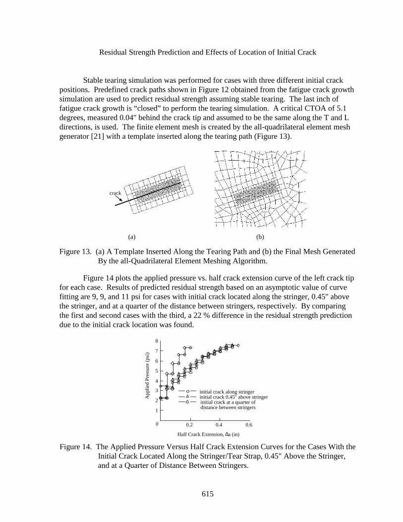
615
Residual Strength Prediction and Effects of Location of Initial Crack
Stable tearing simulation was performed for cases with three different initial crackpositions. Predefined crack paths shown in Figure 12 obtained from the fatigue crack growthsimulation are used to predict residual strength assuming stable tearing. The last inch offatigue crack growth is “closed” to perform the tearing simulation. A critical CTOA of 5.1degrees, measured 0.04" behind the crack tip and assumed to be the same along the T and Ldirections, is used. The finite element mesh is created by the all-quadrilateral element meshgenerator [21] with a template inserted along the tearing path (Figure 13).
crack
Figure 13. (a) A Template Inserted Along the Tearing Path and (b) the Final Mesh GeneratedBy the all-Quadrilateral Element Meshing Algorithm.
Figure 14 plots the applied pressure vs. half crack extension curve of the left crack tipfor each case. Results of predicted residual strength based on an asymptotic value of curvefitting are 9, 9, and 11 psi for cases with initial crack located along the stringer, 0.45" abovethe stringer, and at a quarter of the distance between stringers, respectively. By comparingthe first and second cases with the third, a 22 % difference in the residual strength predictiondue to the initial crack location was found.
.
Half Crack Extension, ∆a (in)
initial crack 0.45" above stringerinitial crack along stringer
initial crack at a quarter ofdistance between stringers
App
lied
Pre
ssur
e (p
si)
0 0.2 0.4 0.6
1
2
3
4
5
6
7
8
Figure 14. The Applied Pressure Versus Half Crack Extension Curves for the Cases With theInitial Crack Located Along the Stringer/Tear Strap, 0.45" Above the Stringer,and at a Quarter of Distance Between Stringers.
(a) (b)
616
CONCLUDING REMARKS
An enhancement of the FRANC3D/STAGS software system with respect to stabletearing simulation for residual strength prediction is presented. For tearing simulations of amiddle crack tension specimen, the predicted residual strength from FRANC3D/STAGSagrees closely with that from the test. However, the relative difference between experimentalmeasurements and the prediction increases as the width of the panels increases. Anengineering approach for shell finite element analysis by utilizing the concept of “planestrain” core to capture the three-dimensional behavior near the tip of the crack is proposed. Abetter agreement with experimental measurements is obtained. However, the validity of thisheuristic approach to general applications other than the M(T) specimen is not clear. Tofurther investigate effects of the crack tip field on residual strength prediction, a fully three-dimensional analysis with a large strain formulation is needed in the future.
Stable tearing simulation of a pressurized fuselage panel, representative of a typicalnarrow-body aircraft, is performed using the predicted crack path obtained from the fatiguecrack growth simulation. The skin is assumed to have 20% higher toughness in the directionperpendicular to the rolling direction than in the rolling direction. The fatigue crack growthdirection criterion based on a simple extrapolation of the maximum tangential stress theory tomaterials with orthotropic toughness is used. Predicted crack growth trajectories agree wellwith the measurements from a full-scale pressurized panel test. Residual strength with theinitial crack located in various positions in the fuselage panel is investigated. Results showedthat a difference in the initial crack location could have significant effects on the residualstrength prediction. In the present study, we (a) neglect the possible trajectory change due tostable tearing, assume (b) that the transition from fatigue to tearing occurs abruptly, and (c)that the plasticity history before the tearing simulation can be ignored. Each of these mighthave significant effects on residual strength prediction and should be investigated in thefuture.
An innovative numerical strategy in simulating fatigue and fracture of an aircraftfuselage has been developed. The close coupling of FRANC3D/STAGS, by combining thegeometric modeling and curvilinear crack growth simulation in FRANC3D with the shellfinite element analysis of STAGS, seeks not only to represent and analyze the problemsfaithfully but also efficiently.
ACKNOWLEDGMENTS
The authors would like to thank Dr. James Newman, Dr. Charles Rankin, Dr. DavidDawicke, Mr. Richard Young, Prof. Alan Zehnder, Dr. Mark Viz, and Dr. Bruce J. Carter formany helpful discussions. This work was performed with support from the NASA LangleyAircraft Structural Integrity Program under contract NAG-1-1184.
617
REFERENCES
1. Potyondy, D. O.: A Software Framework for Simulating Curvilinear Crack Growth inPressurized Thin Shells, Ph.D. Thesis, School of Civil and EnvironmentalEngineering, Cornell University, Ithaca, NY, 1993.
2. Potyondy, D. O., Wawrzynek, P. A., and Ingraffea, A. R.: Discrete Crack GrowthAnalysis Methodology for Through Cracks in Pressurized Fuselage Structures.International Journal for Numerical Methods in Engineering, vol. 38, no. 10, 1995,pp. 1611-1633.
3. Brogan, F. A., Rankin, C. C., and Cabiness, H. D.: STAGS User Manual Version 2.0,1994, Lockheed Palo Alto Research Laboratory, Palo Alto, CA.
4. Dawicke, D. S., Sutton, M. A., Newman Jr., J. C., and Bigelow C. A.: Measurementand Analysis of Critical CTOA for an Aluminum Alloy Sheet, NASA TM-109024,1993.
5. Dawicke, D. S., and Sutton, M. A.: Crack-Tip-Opening Angle Measurement andCrack Tunneling under Stable Tearing in Thin Sheet 2024-T3 Aluminum Alloy,NASA CR-191523, 1993.
6. Newman, J. C., Jr., Bigelow, C. A., and Dawicke, D. S.: Finite-Element Analysesand Fracture Simulation in Thin-Sheet Aluminum Alloy, in Durability of MetalAircraft Structures, Proceedings of the International Workshop on StructuralIntegrity of Aging Airplanes, 1992, Atlanta Technology Publications, Atlanta, GA.
7. Newman, J. C., Jr.: An Elastic-Plastic Finite Element Analysis of Crack Initiation,
Stable Crack Growth, and Instability, in Fracture Mechanics: Fifteen Symposium,ASTM STP 833, 1984.
8. Newman, J. C., Jr., Booth, B. C., and Shivakumar, K. N.: An Elastic-Plastic Finite-Element Analysis of the J-Resistance Curve Using a CTOD Criterion, in FractureMechanics: Eighteen Symposium, ASTM STP 945, 1988, Philadelphia.
9. Newman, J. C., Jr., Dawicke, D. S., Sutton, M. A., and Bigelow, C. A.: A FractureCriterion for Widespread Cracking in Thin-Sheet Aluminum Alloys, in Proc. of the17th Symposium of the International Committee on Aeronautical Fatigue, 1993,Stockholm, Sweden.
10. Zienkiewicz, O. C., and Taylor, R. L.: The Finite Element Method. 4th Ed. Vol. 2,McGraw-Hill Book Company, New York, 1991.
11. Dawicke, D. S.: Personal Communication, 1996.
618
12. Hom, C. L. and McMeeking, R. M.: Large Crack Tip Opening in Thin Elastic-PlasticSheets. International Journal of Fracture, Vol. 45, 1990, pp. 103-122.
13. Hutchinson, J. W.: Singular Behavior at the End of a Tensile Crack in a HardeningMaterial. J. Mech. Phys. Solids, Vol. 16, 1968, pp. 13-31.
14. Rice, J. R. and Rosengren, G. F.: Plane Strain Deformation near a Crack Tip in aPower-Law Hardening Material. J. Mech. Phys. Solids, Vol. 16, 1968, pp. 1-12.
15. Shih, C. F.: Relationships Between the J-Integral and the Crack OpeningDisplacement for Stationary and Extending Cracks. J. Mech. Phys. Solids, Vol. 29,No. 4, 1981, pp. 305-326.
16. Hui, C. Y. and Zehnder, A. T.: A Theory for the Fracture of Thin Plates Subjected toBending and Twisting Moments. International Journal of Fracture, Vol. 61, 1993,pp. 211-229.
17. Viz, M. J., Potyondy, D. O., Zehnder, A. T., Rankin, C. C., and Riks, E.:Computation of Membrane and Bending Stress Intensity Factors for Thin, CrackedPlates. International Journal of Fracture, Vol. 72, 1995, pp. 21-38.
18. Boone, T. J., Wawrzynek, P. A., and Ingraffea, A. R.: Finite Element Modeling ofFracture Propagation in Orthotropic Materials. Engineering Fracture Mechanics,Vol. 26, No. 2, 1987, pp. 185-201.
19. Buczek, M. B., and Herakovich C. T.: A Normal Stress Criterion for CrackExtension Direction in Orthotropic Composite Materials. J. Compos. Mater., Vol. 19,1985, pp. 544-553.
20. Miller, M., Kaelber, K. N., and Worden, R. E.: Finite Element Analysis of PressureVessel Panels, in Durability of Metal Aircraft Structures: Proc. of InternationalWorkshop on Structural Integrity of Aging Airplanes, 1992, Atlanta TechnologyPublications, Atlanta, GA.
21. Potyondy, D. O., Wawrzynek, P. A., and Ingraffea, A. R.: An Algorithm to GenerateQuadrilateral or Triangular Element Surface Meshes in Arbitrary Domains WithApplications to Crack Propagation. International Journal for Numerical Methods inEngineering, vol. 38, 1995, pp. 2677-2701.
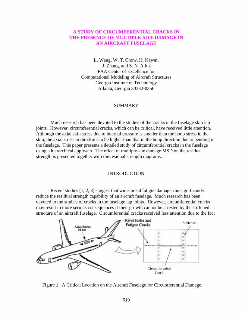
619
A STUDY OF CIRCUMFERENTIAL CRACKS INTHE PRESENCE OF MULTIPLE-SITE DAMAGE IN
AN AIRCRAFT FUSELAGE
L. Wang, W. T. Chow, H. Kawai, J. Zhang, and S. N. Atluri
FAA Center of Excellence forComputational Modeling of Aircraft Structures
Georgia Institute of TechnologyAtlanta, Georgia 30332-0356
SUMMARY
Much research has been devoted to the studies of the cracks in the fuselage skin lapjoints. However, circumferential cracks, which can be critical, have received little attention.Although the axial skin stress due to internal pressure is smaller than the hoop stress in theskin, the axial stress in the skin can be higher than that in the hoop direction due to bending inthe fuselage. This paper presents a detailed study of circumferential cracks in the fuselageusing a hierarchical approach. The effect of multiple-site damage MSD on the residualstrength is presented together with the residual strength diagrams.
INTRODUCTION
Recent studies [1, 2, 3] suggest that widespread fatigue damage can significantlyreduce the residual strength capability of an aircraft fuselage. Much research has beendevoted to the studies of cracks in the fuselage lap joints. However, circumferential cracksmay result in more serious consequences if their growth cannot be arrested by the stiffenedstructure of an aircraft fuselage. Circumferential cracks received less attention due to the fact
Figure 1. A Critical Location on the Aircraft Fuselage for Circumferential Damage.
Stiffener
CircumferentialCrack
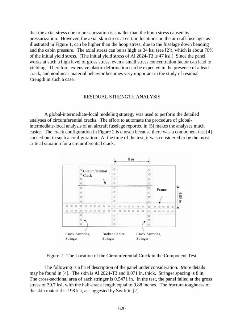
620
that the axial stress due to pressurization is smaller than the hoop stress caused bypressurization. However, the axial skin stress at certain locations on the aircraft fuselage, asillustrated in Figure 1, can be higher than the hoop stress, due to the fuselage down bendingand the cabin pressure. The axial stress can be as high as 34 ksi (see [2]), which is about 70%of the initial yield stress. (The initial yield stress of Al 2024-T3 is 47 ksi.) Since the panelworks at such a high level of gross stress, even a small stress concentration factor can lead toyielding. Therefore, extensive plastic deformation can be expected in the presence of a leadcrack, and nonlinear material behavior becomes very important in the study of residualstrength in such a case.
RESIDUAL STRENGTH ANALYSIS
A global-intermediate-local modeling strategy was used to perform the detailedanalyses of circumferential cracks. The effort to automate the procedure of global-intermediate-local analysis of an aircraft fuselage reported in [5] makes the analyses mucheasier. The crack configuration in Figure 2 is chosen because there was a component test [4]carried out in such a configuration. At the time of the test, it was considered to be the mostcritical situation for a circumferential crack.
Figure 2. The Location of the Circumferential Crack in the Component Test.
The following is a brief description of the panel under consideration. More detailsmay be found in [4]. The skin is Al 2024-T3 and 0.071 in. thick. Stringer spacing is 8 in.The cross-sectional area of each stringer is 0.5471 in. In the test, the panel failed at the grossstress of 39.7 ksi, with the half-crack length equal to 9.88 inches. The fracture toughness ofthe skin material is 198 ksi, as suggested by Swift in [2].
Crack Arresting Broken Center Crack ArrestingStringer Stringer Stringer
CircumferentialCrack
Frame
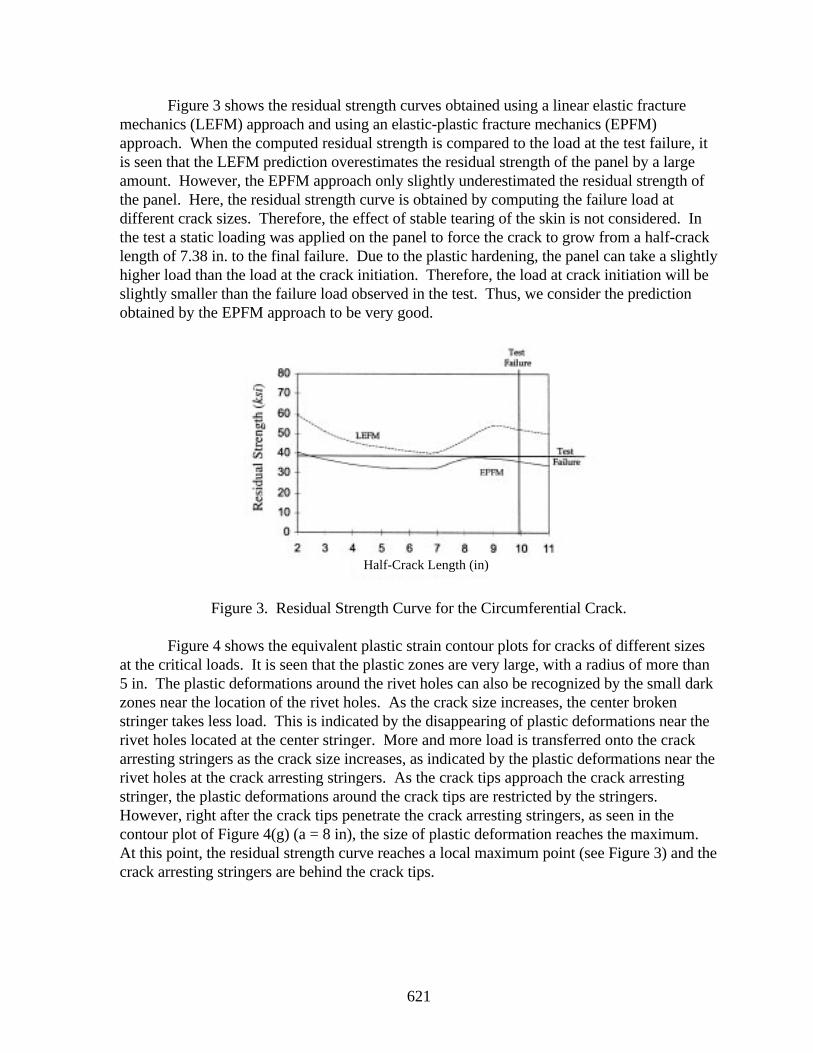
621
Figure 3 shows the residual strength curves obtained using a linear elastic fracturemechanics (LEFM) approach and using an elastic-plastic fracture mechanics (EPFM)approach. When the computed residual strength is compared to the load at the test failure, itis seen that the LEFM prediction overestimates the residual strength of the panel by a largeamount. However, the EPFM approach only slightly underestimated the residual strength ofthe panel. Here, the residual strength curve is obtained by computing the failure load atdifferent crack sizes. Therefore, the effect of stable tearing of the skin is not considered. Inthe test a static loading was applied on the panel to force the crack to grow from a half-cracklength of 7.38 in. to the final failure. Due to the plastic hardening, the panel can take a slightlyhigher load than the load at the crack initiation. Therefore, the load at crack initiation will beslightly smaller than the failure load observed in the test. Thus, we consider the predictionobtained by the EPFM approach to be very good.
Figure 3. Residual Strength Curve for the Circumferential Crack.
Figure 4 shows the equivalent plastic strain contour plots for cracks of different sizesat the critical loads. It is seen that the plastic zones are very large, with a radius of more than5 in. The plastic deformations around the rivet holes can also be recognized by the small darkzones near the location of the rivet holes. As the crack size increases, the center brokenstringer takes less load. This is indicated by the disappearing of plastic deformations near therivet holes located at the center stringer. More and more load is transferred onto the crackarresting stringers as the crack size increases, as indicated by the plastic deformations near therivet holes at the crack arresting stringers. As the crack tips approach the crack arrestingstringer, the plastic deformations around the crack tips are restricted by the stringers.However, right after the crack tips penetrate the crack arresting stringers, as seen in thecontour plot of Figure 4(g) (a = 8 in), the size of plastic deformation reaches the maximum.At this point, the residual strength curve reaches a local maximum point (see Figure 3) and thecrack arresting stringers are behind the crack tips.
Half-Crack Length (in)
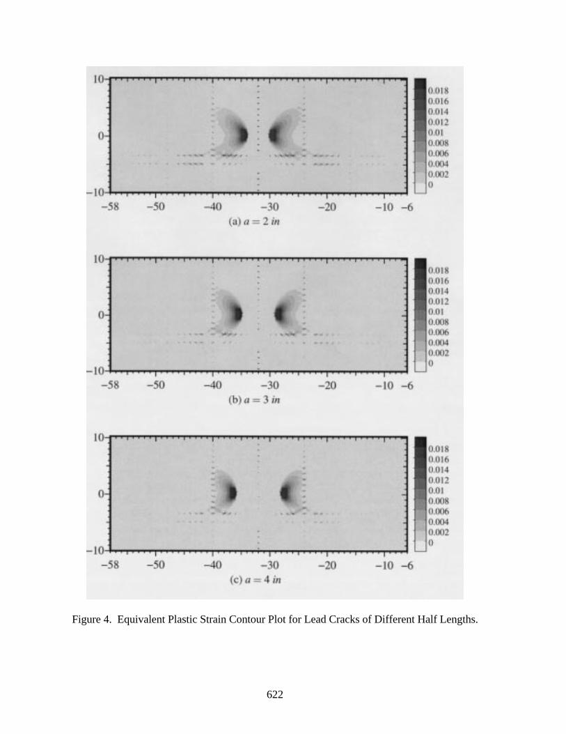
622
Figure 4. Equivalent Plastic Strain Contour Plot for Lead Cracks of Different Half Lengths.
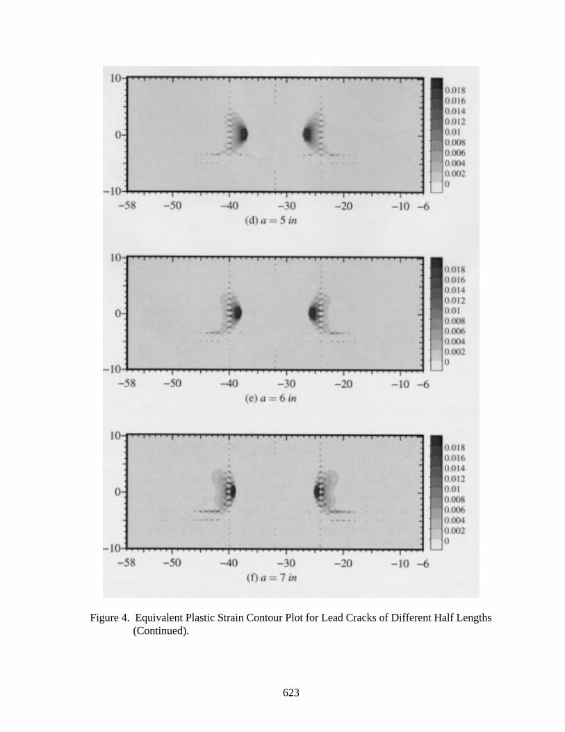
623
Figure 4. Equivalent Plastic Strain Contour Plot for Lead Cracks of Different Half Lengths(Continued).
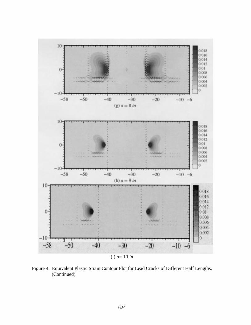
624
(i) a= 10 in
Figure 4. Equivalent Plastic Strain Contour Plot for Lead Cracks of Different Half Lengths.(Continued).

625
Figure 5. The Residual Strength Curves for the Circumferentially Cracked Panel WithFrames of Different Sizes.
Figure 6. The Residual Strength Curves for the Circumferentially Cracked Panel With and Without Cabin Pressure.
The plastic deformations are nearly symmetric about the crack plane for all crack sizes,though they are disturbed near the location of the frame (located below the crack in thecontour plots). This indicates that the effect of the frame is not significant. Figure 5 showsthe residual strength curves for the circumferentially cracked panel with frames of differentsizes. In this analysis, we doubled the size of the frame to study the effect of the frame. It is
Half-Crack Length (in)
Half-Crack Length (in)
WithPressure
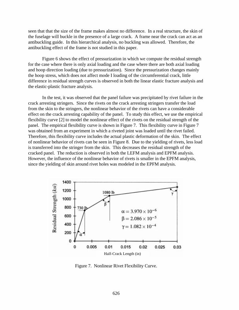
626
seen that that the size of the frame makes almost no difference. In a real structure, the skin ofthe fuselage will buckle in the presence of a large crack. A frame near the crack can act as anantibuckling guide. In this hierarchical analysis, no buckling was allowed. Therefore, theantibuckling effect of the frame is not studied in this paper.
Figure 6 shows the effect of pressurization in which we compute the residual strengthfor the case where there is only axial loading and the case where there are both axial loadingand hoop direction loading (due to pressurization). Since the pressurization changes mainlythe hoop stress, which does not affect mode I loading of the circumferential crack, littledifference in residual strength curves is observed in both the linear elastic fracture analysis andthe elastic-plastic fracture analysis.
In the test, it was observed that the panel failure was precipitated by rivet failure in thecrack arresting stringers. Since the rivets on the crack arresting stringers transfer the loadfrom the skin to the stringers, the nonlinear behavior of the rivets can have a considerableeffect on the crack arresting capability of the panel. To study this effect, we use the empiricalflexibility curve [2] to model the nonlinear effect of the rivets on the residual strength of thepanel. The empirical flexibility curve is shown in Figure 7. This flexibility curve in Figure 7was obtained from an experiment in which a riveted joint was loaded until the rivet failed.Therefore, this flexibility curve includes the actual plastic deformation of the skin. The effectof nonlinear behavior of rivets can be seen in Figure 8. Due to the yielding of rivets, less loadis transferred into the stringer from the skin. This decreases the residual strength of thecracked panel. The reduction is observed in both the LEFM analysis and EPFM analysis.However, the influence of the nonlinear behavior of rivets is smaller in the EPFM analysis,since the yielding of skin around rivet holes was modeled in the EPFM analysis.
Figure 7. Nonlinear Rivet Flexibility Curve.
Half-Crack Length (in)
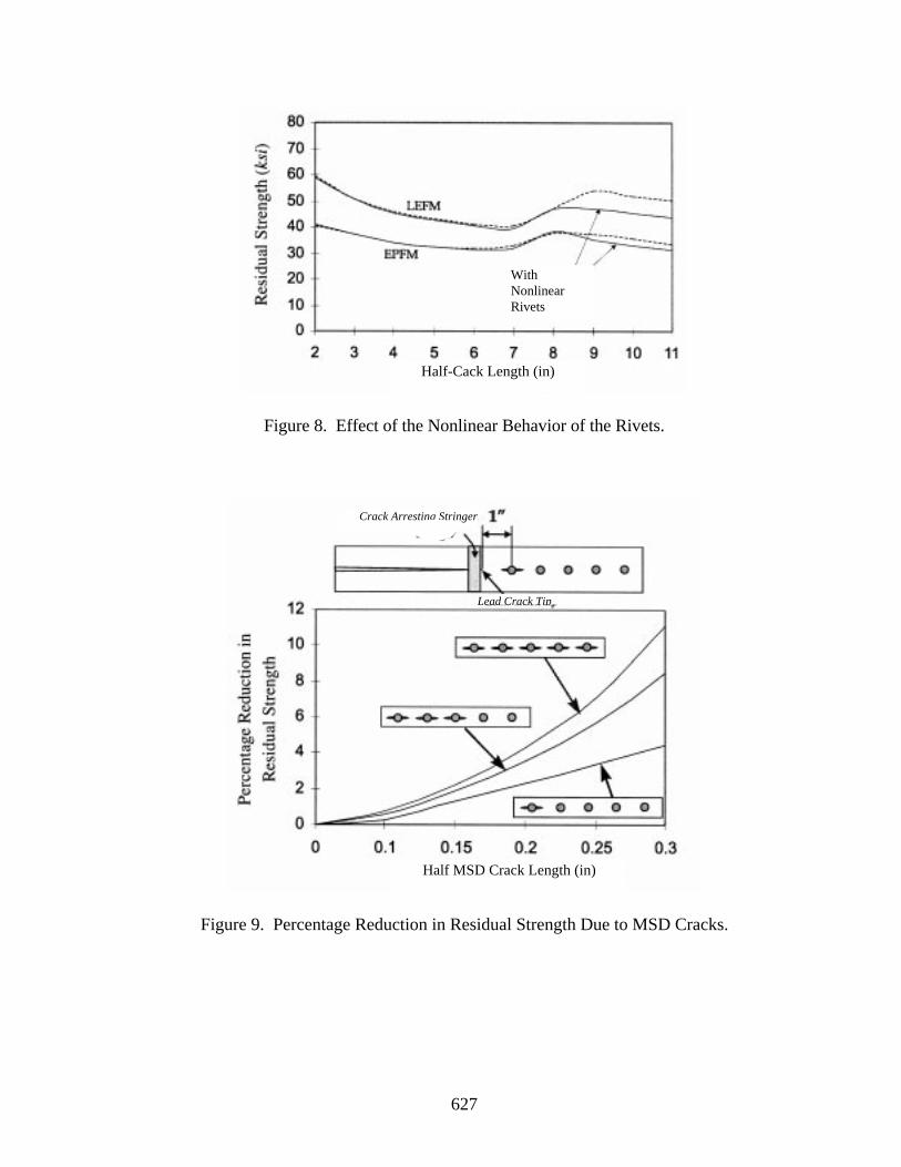
627
Figure 8. Effect of the Nonlinear Behavior of the Rivets.
Figure 9. Percentage Reduction in Residual Strength Due to MSD Cracks.
Half MSD Crack Length (in)
WithNonlinearRivets
Half-Cack Length (in)
Lead Crack Tip
Crack Arresting Stringer
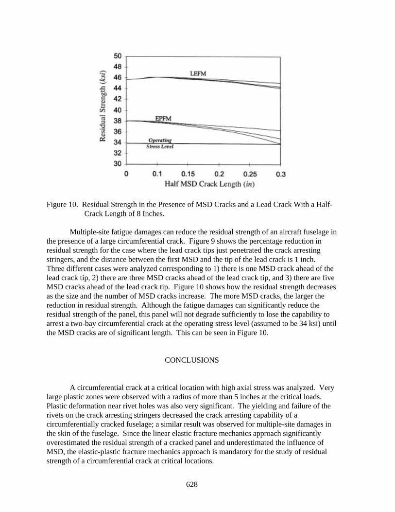
628
Figure 10. Residual Strength in the Presence of MSD Cracks and a Lead Crack With a Half-Crack Length of 8 Inches.
Multiple-site fatigue damages can reduce the residual strength of an aircraft fuselage inthe presence of a large circumferential crack. Figure 9 shows the percentage reduction inresidual strength for the case where the lead crack tips just penetrated the crack arrestingstringers, and the distance between the first MSD and the tip of the lead crack is 1 inch.Three different cases were analyzed corresponding to 1) there is one MSD crack ahead of thelead crack tip, 2) there are three MSD cracks ahead of the lead crack tip, and 3) there are fiveMSD cracks ahead of the lead crack tip. Figure 10 shows how the residual strength decreasesas the size and the number of MSD cracks increase. The more MSD cracks, the larger thereduction in residual strength. Although the fatigue damages can significantly reduce theresidual strength of the panel, this panel will not degrade sufficiently to lose the capability toarrest a two-bay circumferential crack at the operating stress level (assumed to be 34 ksi) untilthe MSD cracks are of significant length. This can be seen in Figure 10.
CONCLUSIONS
A circumferential crack at a critical location with high axial stress was analyzed. Verylarge plastic zones were observed with a radius of more than 5 inches at the critical loads.Plastic deformation near rivet holes was also very significant. The yielding and failure of therivets on the crack arresting stringers decreased the crack arresting capability of acircumferentially cracked fuselage; a similar result was observed for multiple-site damages inthe skin of the fuselage. Since the linear elastic fracture mechanics approach significantlyoverestimated the residual strength of a cracked panel and underestimated the influence ofMSD, the elastic-plastic fracture mechanics approach is mandatory for the study of residualstrength of a circumferential crack at critical locations.
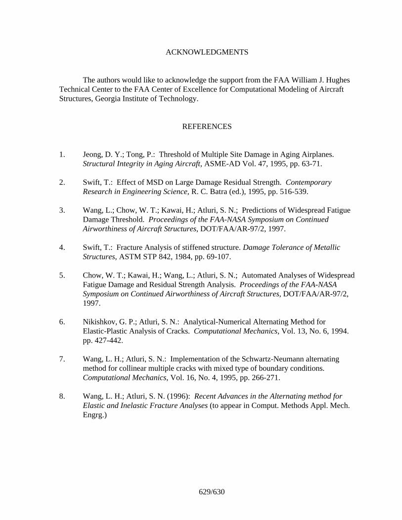
629/630
ACKNOWLEDGMENTS
The authors would like to acknowledge the support from the FAA William J. HughesTechnical Center to the FAA Center of Excellence for Computational Modeling of AircraftStructures, Georgia Institute of Technology.
REFERENCES
1. Jeong, D. Y.; Tong, P.: Threshold of Multiple Site Damage in Aging Airplanes.Structural Integrity in Aging Aircraft, ASME-AD Vol. 47, 1995, pp. 63-71.
2. Swift, T.: Effect of MSD on Large Damage Residual Strength. Contemporary
Research in Engineering Science, R. C. Batra (ed.), 1995, pp. 516-539. 3. Wang, L.; Chow, W. T.; Kawai, H.; Atluri, S. N.; Predictions of Widespread Fatigue
Damage Threshold. Proceedings of the FAA-NASA Symposium on ContinuedAirworthiness of Aircraft Structures, DOT/FAA/AR-97/2, 1997.
4. Swift, T.: Fracture Analysis of stiffened structure. Damage Tolerance of Metallic
Structures, ASTM STP 842, 1984, pp. 69-107. 5. Chow, W. T.; Kawai, H.; Wang, L.; Atluri, S. N.; Automated Analyses of Widespread
Fatigue Damage and Residual Strength Analysis. Proceedings of the FAA-NASASymposium on Continued Airworthiness of Aircraft Structures, DOT/FAA/AR-97/2,1997.
6. Nikishkov, G. P.; Atluri, S. N.: Analytical-Numerical Alternating Method for
Elastic-Plastic Analysis of Cracks. Computational Mechanics, Vol. 13, No. 6, 1994.pp. 427-442.
7. Wang, L. H.; Atluri, S. N.: Implementation of the Schwartz-Neumann alternating
method for collinear multiple cracks with mixed type of boundary conditions.Computational Mechanics, Vol. 16, No. 4, 1995, pp. 266-271.
8. Wang, L. H.; Atluri, S. N. (1996): Recent Advances in the Alternating method for
Elastic and Inelastic Fracture Analyses (to appear in Comput. Methods Appl. Mech.Engrg.)
631
A STUDY OF FATIGUE CRACK GENERATION ANDGROWTH IN RIVETED ALCLAD 2024-T3 S PECIMENS
Z. M. Connor, M. E. Fine, and B. MoranNorthwestern University
Department of Materials ScienceEvanston, Illinois 60208
SUMMARY
Initiation and propagation of fatigue cracks at rivets in Alclad 2024-T3 specimenswere investigated microscopically. Fatigue tests were performed on five identical specimens.Each specimen was assembled from two pieces of Alclad 2024-T3 sheet material using three2017T4 aluminum alloy rivets. One piece of the sheet material had three countersunk rivetholes and the mating sheet had three straight holes. The specimens were loaded in uniaxialtension with a maximum load of 4.0 kN and an R ratio of 0.1. The number of cycles until acrack approximately 2 mm in length was seen in the plate near the rivet head was defined asNi. The average Ni was 310,000 cycles with a standard deviation of 80,000 cycles. A surfacerumpling consisting of plastic deformation and microcracks is observed adjacent to the rivethead prior to emergence of a propagating crack. Both circumferential and radial microcracksare seen. Using a 40 times magnification microscope, the propagating cracks were 0.5 to 1.7mm long when first observed. In many specimens, such cracks did not grow significantly formany cycles after first observed. The time period between when surface rumpling is firstobserved and the end of the slow crack growth may provide a window of opportunity forearly crack detection. This is a useful method for preparing specimens for nondestructiveevaluation (NDE) calibration.
INTRODUCTION
Prior to investigating fatigue crack initiation and propagation in riveted joints,uniaxially loaded specimens of Alclad 2024 T3 aluminum alloy with countersunk rivet holeswere investigated microscopically. A significant variation was observed in the cycles toinitiation of a detectable crack under closely controlled conditions that were intended to beidentical. The holes were made with a computer controlled machine tool and the maximumand minimum loads in the fatigue cycle were constant. The fatigue cracks initiated asmicrocracks in the blunt knife edges of the countersunk rivet holes and then extended asMode I cracks [1-3]. This present paper reports the results on lap joint specimens consistingof two panels fastened with three rivets aligned in the stress direction and loaded in uniaxialtension.
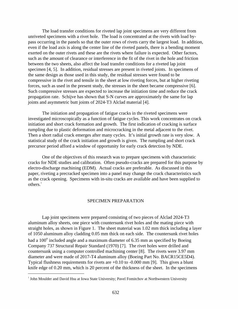
632
The load transfer conditions for riveted lap joint specimens are very different fromunriveted specimens with a rivet hole. The load is concentrated at the rivets with load by-pass occurring in the panels so that the outer rows of rivets carry the largest load. In addition,even if the load axis is along the center line of the riveted panels, there is a bending momentexerted on the outer rivets and these are the rivets where failure is expected. Other factors,such as the amount of clearance or interference in the fit of the rivet in the hole and frictionbetween the two sheets, also affect the load transfer conditions for a riveted lap jointspecimen [4, 5]. In addition, residual stresses are present in riveted joints. In specimens ofthe same design as those used in this study, the residual stresses were found to becompressive in the rivet and tensile in the sheet at low riveting forces, but at higher rivetingforces, such as used in the present study, the stresses in the sheet became compressive [6].Such compressive stresses are expected to increase the initiation time and reduce the crackpropagation rate. Schijve has shown that S-N curves are approximately the same for lapjoints and asymmetric butt joints of 2024-T3 Alclad material [4].
The initiation and propagation of fatigue cracks in the riveted specimens wereinvestigated microscopically as a function of fatigue cycles. This work concentrates on crackinitiation and short crack formation and growth. The first indication of cracking is surfacerumpling due to plastic deformation and microcracking in the metal adjacent to the rivet.Then a short radial crack emerges after many cycles. It’s initial growth rate is very slow. Astatistical study of the crack initiation and growth is given. The rumpling and short crackprecursor period afford a window of opportunity for early crack detection by NDE.
One of the objectives of this research was to prepare specimens with characteristiccracks for NDE studies and calibration. Often pseudo-cracks are prepared for this purpose byelectro-discharge machining (EDM). Actual cracks are preferable. As discussed in thispaper, riveting a precracked specimen into a panel may change the crack characteristics suchas the crack opening. Specimens with in-situ cracks are available and have been supplied toothers.1
SPECIMEN PREPARATION
Lap joint specimens were prepared consisting of two pieces of Alclad 2024-T3aluminum alloy sheets, one piece with countersunk rivet holes and the mating piece withstraight holes, as shown in Figure 1. The sheet material was 1.02 mm thick including a layerof 1050 aluminum alloy cladding 0.05 mm thick on each side. The countersunk rivet holes
had a 100o included angle and a maximum diameter of 6.35 mm as specified by BoeingCompany 737 Structural Repair Standard (1970) [7]. The rivet holes were drilled andcountersunk using a computer controlled machining center [8]. The rivets were 3.97 mmdiameter and were made of 2017-T4 aluminum alloy (Boeing Part No. BACR15CE5D4).Typical flushness requirements for rivets are +0.10 to -0.000 mm [9]. This gives a bluntknife edge of 0.20 mm, which is 20 percent of the thickness of the sheet. In the specimens 1 John Moulder and David Hsu at Iowa State University; Pavel Fomitchov at Northwestern University
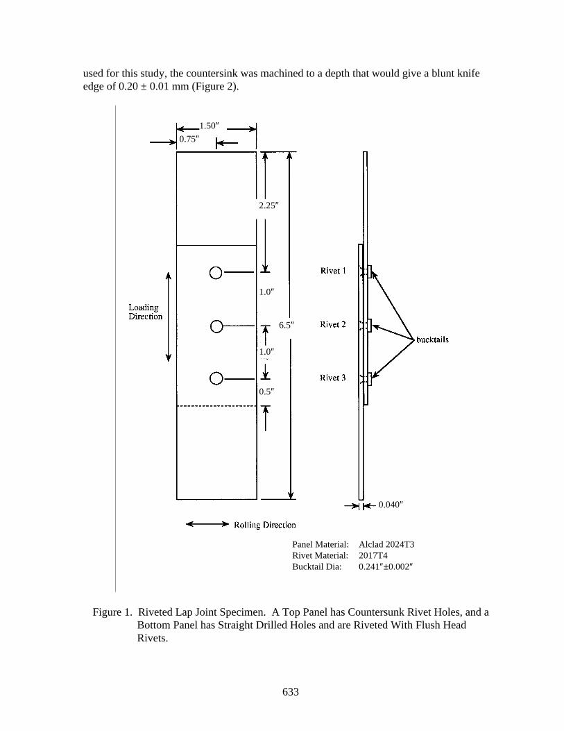
633
used for this study, the countersink was machined to a depth that would give a blunt knifeedge of 0.20 ± 0.01 mm (Figure 2).
Figure 1. Riveted Lap Joint Specimen. A Top Panel has Countersunk Rivet Holes, and aBottom Panel has Straight Drilled Holes and are Riveted With Flush HeadRivets.
0.5″
0.040″
Panel Material: Alclad 2024T3Rivet Material: 2017T4Bucktail Dia: 0.241″±0.002″
1.0″
6.5″
1.0″
2.25″
1.50″0.75″
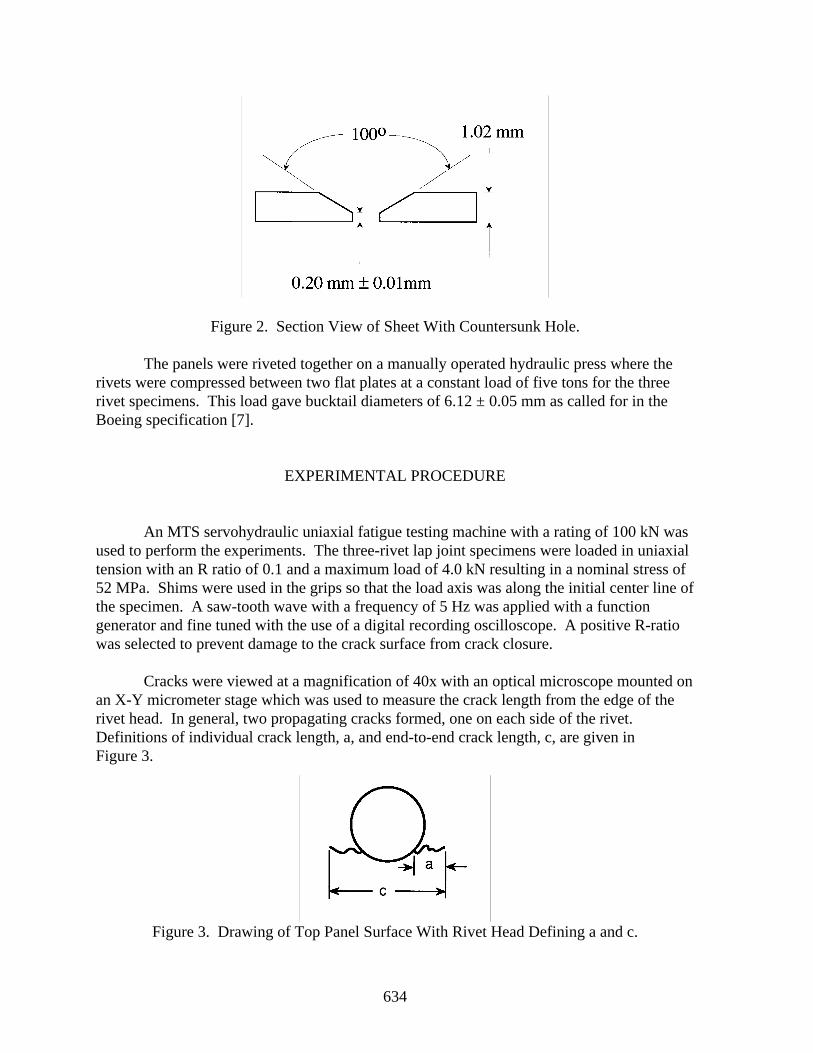
634
Figure 2. Section View of Sheet With Countersunk Hole.
The panels were riveted together on a manually operated hydraulic press where therivets were compressed between two flat plates at a constant load of five tons for the threerivet specimens. This load gave bucktail diameters of 6.12 ± 0.05 mm as called for in theBoeing specification [7].
EXPERIMENTAL PROCEDURE
An MTS servohydraulic uniaxial fatigue testing machine with a rating of 100 kN wasused to perform the experiments. The three-rivet lap joint specimens were loaded in uniaxialtension with an R ratio of 0.1 and a maximum load of 4.0 kN resulting in a nominal stress of52 MPa. Shims were used in the grips so that the load axis was along the initial center line ofthe specimen. A saw-tooth wave with a frequency of 5 Hz was applied with a functiongenerator and fine tuned with the use of a digital recording oscilloscope. A positive R-ratiowas selected to prevent damage to the crack surface from crack closure.
Cracks were viewed at a magnification of 40x with an optical microscope mounted onan X-Y micrometer stage which was used to measure the crack length from the edge of therivet head. In general, two propagating cracks formed, one on each side of the rivet.Definitions of individual crack length, a, and end-to-end crack length, c, are given inFigure 3.
Figure 3. Drawing of Top Panel Surface With Rivet Head Defining a and c.
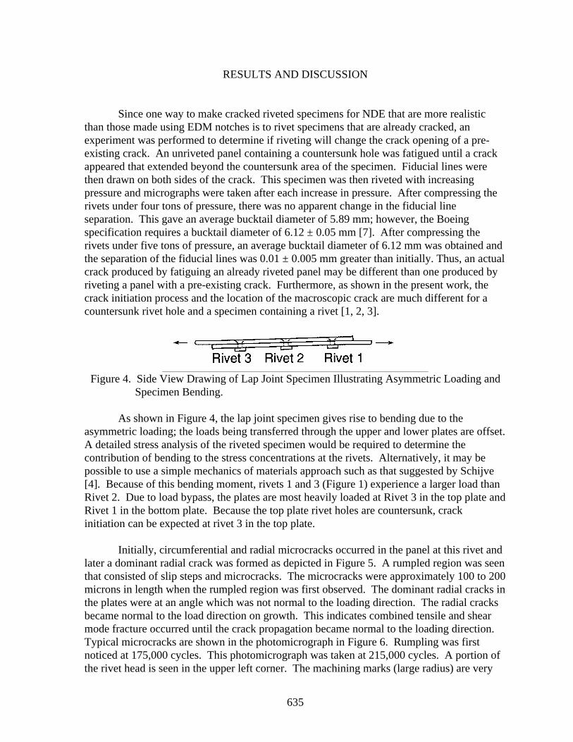
635
RESULTS AND DISCUSSION
Since one way to make cracked riveted specimens for NDE that are more realisticthan those made using EDM notches is to rivet specimens that are already cracked, anexperiment was performed to determine if riveting will change the crack opening of a pre-existing crack. An unriveted panel containing a countersunk hole was fatigued until a crackappeared that extended beyond the countersunk area of the specimen. Fiducial lines werethen drawn on both sides of the crack. This specimen was then riveted with increasingpressure and micrographs were taken after each increase in pressure. After compressing therivets under four tons of pressure, there was no apparent change in the fiducial lineseparation. This gave an average bucktail diameter of 5.89 mm; however, the Boeingspecification requires a bucktail diameter of 6.12 ± 0.05 mm [7]. After compressing therivets under five tons of pressure, an average bucktail diameter of 6.12 mm was obtained andthe separation of the fiducial lines was 0.01 ± 0.005 mm greater than initially. Thus, an actualcrack produced by fatiguing an already riveted panel may be different than one produced byriveting a panel with a pre-existing crack. Furthermore, as shown in the present work, thecrack initiation process and the location of the macroscopic crack are much different for acountersunk rivet hole and a specimen containing a rivet [1, 2, 3].
Figure 4. Side View Drawing of Lap Joint Specimen Illustrating Asymmetric Loading andSpecimen Bending.
As shown in Figure 4, the lap joint specimen gives rise to bending due to theasymmetric loading; the loads being transferred through the upper and lower plates are offset.A detailed stress analysis of the riveted specimen would be required to determine thecontribution of bending to the stress concentrations at the rivets. Alternatively, it may bepossible to use a simple mechanics of materials approach such as that suggested by Schijve[4]. Because of this bending moment, rivets 1 and 3 (Figure 1) experience a larger load thanRivet 2. Due to load bypass, the plates are most heavily loaded at Rivet 3 in the top plate andRivet 1 in the bottom plate. Because the top plate rivet holes are countersunk, crackinitiation can be expected at rivet 3 in the top plate.
Initially, circumferential and radial microcracks occurred in the panel at this rivet andlater a dominant radial crack was formed as depicted in Figure 5. A rumpled region was seenthat consisted of slip steps and microcracks. The microcracks were approximately 100 to 200microns in length when the rumpled region was first observed. The dominant radial cracks inthe plates were at an angle which was not normal to the loading direction. The radial cracksbecame normal to the load direction on growth. This indicates combined tensile and shearmode fracture occurred until the crack propagation became normal to the loading direction.Typical microcracks are shown in the photomicrograph in Figure 6. Rumpling was firstnoticed at 175,000 cycles. This photomicrograph was taken at 215,000 cycles. A portion ofthe rivet head is seen in the upper left corner. The machining marks (large radius) are very
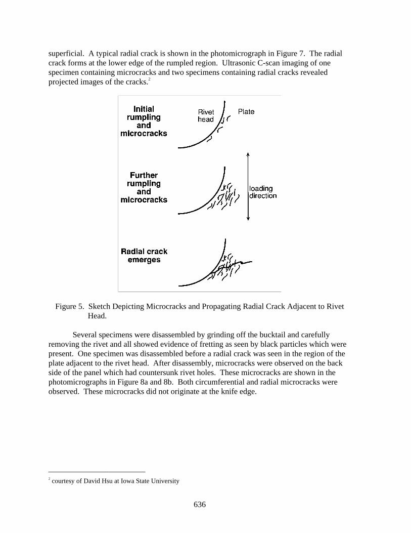
636
superficial. A typical radial crack is shown in the photomicrograph in Figure 7. The radialcrack forms at the lower edge of the rumpled region. Ultrasonic C-scan imaging of onespecimen containing microcracks and two specimens containing radial cracks revealedprojected images of the cracks.2
Figure 5. Sketch Depicting Microcracks and Propagating Radial Crack Adjacent to RivetHead.
Several specimens were disassembled by grinding off the bucktail and carefullyremoving the rivet and all showed evidence of fretting as seen by black particles which werepresent. One specimen was disassembled before a radial crack was seen in the region of theplate adjacent to the rivet head. After disassembly, microcracks were observed on the backside of the panel which had countersunk rivet holes. These microcracks are shown in thephotomicrographs in Figure 8a and 8b. Both circumferential and radial microcracks wereobserved. These microcracks did not originate at the knife edge.
2 courtesy of David Hsu at Iowa State University
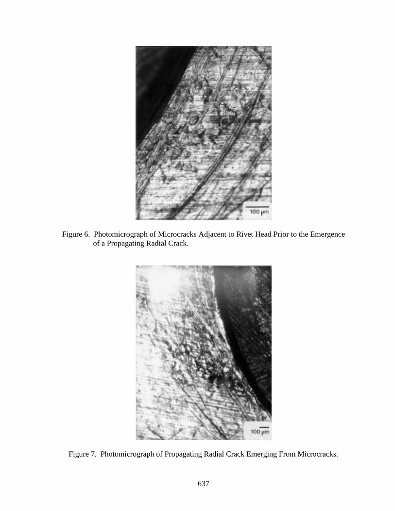
637
Figure 6. Photomicrograph of Microcracks Adjacent to Rivet Head Prior to the Emergenceof a Propagating Radial Crack.
Figure 7. Photomicrograph of Propagating Radial Crack Emerging From Microcracks.
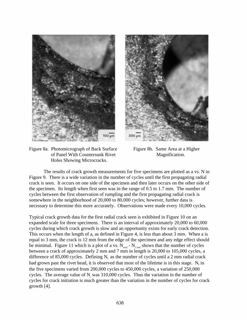
638
Figure 8a. Photomicrograph of Back Surfaceof Panel With Countersunk RivetHoles Showing Microcracks.
Figure 8b. Same Area at a HigherMagnification.
The results of crack growth measurements for five specimens are plotted as a vs. N inFigure 9. There is a wide variation in the number of cycles until the first propagating radialcrack is seen. It occurs on one side of the specimen and then later occurs on the other side ofthe specimen. Its length when first seen was in the range of 0.5 to 1.7 mm. The number ofcycles between the first observation of rumpling and the first propagating radial crack issomewhere in the neighborhood of 20,000 to 80,000 cycles; however, further data isnecessary to determine this more accurately. Observations were made every 10,000 cycles.
Typical crack growth data for the first radial crack seen is exhibited in Figure 10 on anexpanded scale for three specimens. There is an interval of approximately 20,000 to 60,000cycles during which crack growth is slow and an opportunity exists for early crack detection.This occurs when the length of a, as defined in Figure 4, is less than about 3 mm. When a isequal to 3 mm, the crack is 12 mm from the edge of the specimen and any edge effect shouldbe minimal. Figure 11 which is a plot of a vs. Ntotal - N2 mm shows that the number of cyclesbetween a crack of approximately 2 mm and 7 mm in length is 20,000 to 105,000 cycles, adifference of 85,000 cycles. Defining Ni as the number of cycles until a 2 mm radial crackhad grown past the rivet head, it is observed that most of the lifetime is in this stage. Ni inthe five specimens varied from 200,000 cycles to 450,000 cycles, a variation of 250,000cycles. The average value of Ni was 310,000 cycles. Thus the variation in the number ofcycles for crack initiation is much greater than the variation in the number of cycles for crackgrowth [4].
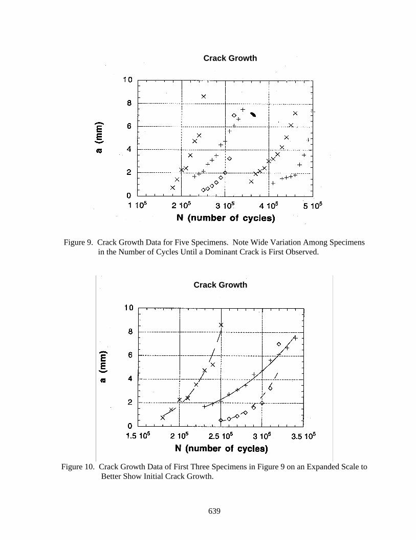
639
Figure 9. Crack Growth Data for Five Specimens. Note Wide Variation Among Specimensin the Number of Cycles Until a Dominant Crack is First Observed.
Figure 10. Crack Growth Data of First Three Specimens in Figure 9 on an Expanded Scale toBetter Show Initial Crack Growth.
Crack Growth
Crack Growth
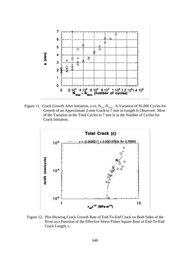
640
Figure 11. Crack Growth After Initiation, a vs. Ntotal-N2mm. A Variation of 85,000 Cycles forGrowth of an Approximate 2-mm Crack to 7 mm in Length Is Observed. Mostof the Variation in the Total Cycles to 7 mm Is in the Number of Cycles forCrack Initiation.
Figure 12. Plot Showing Crack Growth Rate of End-To-End Crack on Both Sides of theRivet as a Function of the Effective Stress Times Square Root of End-To-EndCrack Length, c.
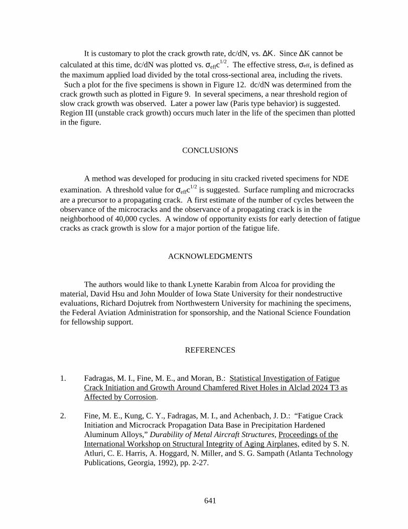
641
It is customary to plot the crack growth rate, dc/dN, vs. ∆Κ. Since ∆K cannot be
calculated at this time, dc/dN was plotted vs. σeffc1/2. The effective stress, σeff, is defined as
the maximum applied load divided by the total cross-sectional area, including the rivets. Such a plot for the five specimens is shown in Figure 12. dc/dN was determined from thecrack growth such as plotted in Figure 9. In several specimens, a near threshold region ofslow crack growth was observed. Later a power law (Paris type behavior) is suggested.Region III (unstable crack growth) occurs much later in the life of the specimen than plottedin the figure.
CONCLUSIONS
A method was developed for producing in situ cracked riveted specimens for NDE
examination. A threshold value for σeffc1/2 is suggested. Surface rumpling and microcracks
are a precursor to a propagating crack. A first estimate of the number of cycles between theobservance of the microcracks and the observance of a propagating crack is in theneighborhood of 40,000 cycles. A window of opportunity exists for early detection of fatiguecracks as crack growth is slow for a major portion of the fatigue life.
ACKNOWLEDGMENTS
The authors would like to thank Lynette Karabin from Alcoa for providing thematerial, David Hsu and John Moulder of Iowa State University for their nondestructiveevaluations, Richard Dojutrek from Northwestern University for machining the specimens,the Federal Aviation Administration for sponsorship, and the National Science Foundationfor fellowship support.
REFERENCES
1. Fadragas, M. I., Fine, M. E., and Moran, B.: Statistical Investigation of FatigueCrack Initiation and Growth Around Chamfered Rivet Holes in Alclad 2024 T3 asAffected by Corrosion.
2. Fine, M. E., Kung, C. Y., Fadragas, M. I., and Achenbach, J. D.: “Fatigue Crack
Initiation and Microcrack Propagation Data Base in Precipitation HardenedAluminum Alloys,” Durability of Metal Aircraft Structures, Proceedings of theInternational Workshop on Structural Integrity of Aging Airplanes, edited by S. N.Atluri, C. E. Harris, A. Hoggard, N. Miller, and S. G. Sampath (Atlanta TechnologyPublications, Georgia, 1992), pp. 2-27.
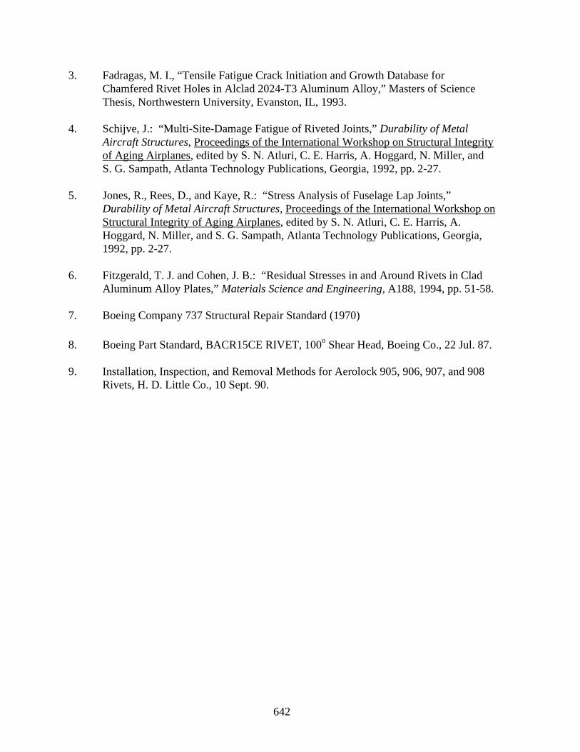
642
3. Fadragas, M. I., “Tensile Fatigue Crack Initiation and Growth Database forChamfered Rivet Holes in Alclad 2024-T3 Aluminum Alloy,” Masters of ScienceThesis, Northwestern University, Evanston, IL, 1993.
4. Schijve, J.: “Multi-Site-Damage Fatigue of Riveted Joints,” Durability of Metal
Aircraft Structures, Proceedings of the International Workshop on Structural Integrityof Aging Airplanes, edited by S. N. Atluri, C. E. Harris, A. Hoggard, N. Miller, andS. G. Sampath, Atlanta Technology Publications, Georgia, 1992, pp. 2-27.
5. Jones, R., Rees, D., and Kaye, R.: “Stress Analysis of Fuselage Lap Joints,”
Durability of Metal Aircraft Structures, Proceedings of the International Workshop onStructural Integrity of Aging Airplanes, edited by S. N. Atluri, C. E. Harris, A.Hoggard, N. Miller, and S. G. Sampath, Atlanta Technology Publications, Georgia,1992, pp. 2-27.
6. Fitzgerald, T. J. and Cohen, J. B.: “Residual Stresses in and Around Rivets in Clad
Aluminum Alloy Plates,” Materials Science and Engineering, A188, 1994, pp. 51-58. 7. Boeing Company 737 Structural Repair Standard (1970)
8. Boeing Part Standard, BACR15CE RIVET, 100o Shear Head, Boeing Co., 22 Jul. 87. 9. Installation, Inspection, and Removal Methods for Aerolock 905, 906, 907, and 908
Rivets, H. D. Little Co., 10 Sept. 90.
643
T* ε INTEGRALS FOR CURVED CRACK GROWTH *
P. W. Lam and A. S. KobayashiUniversity of WashingtonSeattle, WA 98195-2600
H. Okada and S. N. AtluriGeorgia Institute of Technology
Atlanta, GA 30332-0356
P. W. TanFederal Aviation Administration
William J. Hughes Technical CenterAtlantic City International Airport, NJ 08405
SUMMARY
T*ε integral values associated with a stable, curved crack growth in biaxially loaded,fatigued precracked, 2024-T3 single edge notched (SEN) specimens, which were loaded in acombined modes I and II loading, were determined. These SEN specimens mimicked theflapping of a failed lap slice of a pressurized airplane fuselage. Most specimens wereoutfitted with a tear strap, which was either bonded, bonded and riveted, or integrallymachined in the specimen. The crack curved upon propagation due to the imposed mode IIcrack tip deformation and either penetrated or curved again upon hitting the tear strap. T*1εintegral was identical to that of mode I crack extension while T*2ε vanished. In general, thecrack curved in the direction of maximum principal strain.
INTRODUCTION
When a pre-existing axial crack in a lap slice of a pressurized fuselage extends undercritical load, the flap generated by the one-sided bulging will tend to tear away from the lapjoint. The mechanism of this flap generation was attributed to the imposed mode II stressintensity factor, KII,, induced by the characteristic one-sided bulging peculiar to a lap splicejoint failure and results in an abrupt crack kinking away from the axial direction. This crackkinking was analyzed in detail by Kosai, et al. [1-3] using linear elastic fracture mechanicsdespite the presence of considerable large-scale plastic yielding. This plastic yielding is often
* This study is supported by FAA research grants to the Georgia Institute of Technology and to the
University of Washington, FAA Grant No. 92-G-0005.
644
compounded by the presence of multisite damage (MSD) which links up with the main axialcrack through plastic collapse [4]. After kinking, the crack normally propagates diagonallyuntil it approaches a tear strap or a frame after which it most likely will kink again andpropagate circumferentially until the driving force, i.e., fuselage pressure, has beenexhausted. Again, the numerical analyses of Kosai, et al. [1 - 3] exhibited considerableplastic yielding during the propagation phase of the kinked crack. The above brief reviewshows that while linear elastic fracture mechanics (LEFM) techniques can be usedeffectively, particularly in an industrial setting, to predict crack kinking in a lap joint and at acrack arrestor, the fracture mechanic-based prediction technique can be improved byincorporating the plasticity effect in the analysis.
This paper presents our initial effort toward the development of an elastic-plasticcrack curving criterion. T*ε integral, which has been used successfully by the authors andtheir colleagues in analyzing mode I, stable and dynamic ductile crack growth [5 - 7], will beused in assessing crack curving in the presence of large-scale yielding.
THEORETICAL BACKGROUND
T*ε is a path dependent integral based on incremental theory of plasticity where theintegration contour expands together with the extending crack [8,9]. By confining theintegration contour, Γε, to the very vicinity of a traction-free crack and by using the stress andstrain fields generated by the incremental theory of plasticity, Okada and Atluri [10] haveshown that T*ε can be computed by the current T*ε without the need to sum ∆T* ε for eachincremental crack extension. Moreover, the trailing portion of the contour integral can beignored since the resultant surface tractions acting on such near-crack contours vanish. Thisnearness, ε, is set to the thickness of the specimen in order to guarantee a state of plane stressalong the integration contour, Γε [11].
Without the contour integration involving the unloaded region, the contour integralahead of the crack tip can be evaluated by using the deformation theory of plasticity since thisfrontal region is dominated by the loading process. Thus the experimentally impracticalprocedure of evaluating ∆T* ε is avoided and T*ε was determined directly from the measureddisplacement field surrounding a partial contour near and in front of the crack tip. This isfortunate since the state of stress based on the incremental theory of plasticity cannot bereadily computed from the measured displacement and strain fields in the trailing crack wakeregion. The T*ε for this near field Γε represents the energy flux into a strip parallel to thecrack as shown also by Memhard, et al. [12].
For a straight crack, which is subjected to a mixed modes I and II crack tipdeformation, as is the case of the initial phase of a lap joint failure, the two modes of the T*kεfor self-similar straight crack propagation are
645
T*kε = ∫ [ W n k − σij ni ui,k] dΓ (1)Γε
where k = 1 and 2 represent the crack tip deformation of modes I and II, respectively, and i, j= 1, 2. For mode I, T*kε vanishes in the trailing crack wake since n1 = 0 and σ12 ≈ σ22 ≈ 0very close to the traction-free crack. For mode II, only the W term contributes to T*kε alongthe crack wake.
For a curved crack, the energy flux into an elongated curved contour will require theevaluation of T*kε along the entire contour, including the crack wake region, as well as anadditional term which accounts for the rotation of the curved crack. Thus for a curved crack,a locally self-similar crack field, as shown in Fig. 1, where T*kε, as represented by Eq. 1, isevaluated along a near-crack contour, Γε, which surrounds only the frontal region of thegrowing crack tip and does not extend back to the original crack tip location.
EXPERIMENTAL ANALYSIS
Biaxial SEN Specimen
The mode II crack tip deformation generated by the unsymmetric flap opening alongthe lap joint in a rupturing pressurized fuselage was simulated by an in-plane shear loadingalong a single edge crack. Figure 2 show the basic configuration of the biaxial fracturespecimen which is similar in design with that used by Kosai, et al. [13]. The x- and y-direction loads, Px and Py, were applied through pin-loaded heavy steel grips. Py simulatesthe hoop stress of the fuselage and the load parallel to the crack, i.e., the x-direction load, Px,simulates the unsymmetric axial stress generated by the opening flap. This axial stress wasidentified as the dominant force which caused crack curving in a pressurized fuselage [1 - 3].The upper load, Px1, which is twice the lower load, Px2, simulated the unequal axial loadimposed by the one-sided flapping of the fuselage skin as the crack propagated axially alonga fuselage lap joint. The specimen was fatigue precracked under uniaxial cyclic loading. Atear strap was either epoxy bonded, bonded and riveted at spacing 12.5 mm apart, orintegrally machined onto the specimen at the far edge.
646
Test Procedure
The test section of the specimen was covered with a crossed Moiré diffraction gratingof 40 lines/mm over a region of 50 x 50 mm. This coarse Moiré grating was necessary due tothe large-scale plastic yielding, which resulted in Moiré fringe patterns too dense to resolveby the traditional high-density grating. The grating was transferred onto the highly polishedspecimen surface by contact printing a master grating on to a relatively thick photo-resistcoating which was deposited onto the specimen surface [14]. The deep cross-grooved,photoresist coating and the exposed, highly reflective specimen surface constituted adiffraction grating which withstood the large straining in the crack tip region. The specimenwas illuminated by a four-beam Moiré interferometer for sequential recording of the twoMoiré interferometry fringe patterns, which correspond to the two orthogonal displacementfields and which, unlike the traditional Moiré interferometry, could be viewed from anyangular orientation [15].
The specimen was loaded in a biaxial testing machine with fixed grip loadingconditions, ∆x and ∆y. The test protocol consisted of gradually increasing ∆x and ∆y whilerecording the Moiré fringe patterns associated with curved crack growth. The unsymmetric x-direction load at the left tab of the biaxial fracture specimen was generated by a simplemechanical lever system at the side of the cruciform specimen which provided a fixed upper-to-lower load ratio of Px1/Px2= 2. The two time-varying loads, i.e., Px and Py, were
measured with two load cells and the imposed fixed grip loading, ∆x and ∆y, were measuredby linear variable transducers.
RESULTS
Twenty-four biaxial test specimens were fabricated without or with tear straps andthese results are being evaluated. We report in this paper the results obtained in onespecimen with a bonded tear strap. Figure 3 shows the Moiré fringe patterns correspondingto the u- and v-displacements, respectively, in the biaxial test specimen with a curving crackpath. Here the u- and v-fields refer to the displacements parallel and perpendicular to thecrack, respectively.
Figure 4 shows the curved crack which for analysis purpose is represented bysegments of straight cracks. Also shown is the frontal portion of the Γε contour of ε = 0.8mm (specimen thickness) in front of the extended curved crack.
Figure 5 shows the T*kε, which were determined by evaluating the contour integral ofEq. 1, along the frontal portion of Γε at the seven crack tip locations of the curved crack. Thenumerical procedure described in Reference 10 were used to deduce T*kε from the u- and v-displacement fields obtained from the corresponding seven sets of Moiré fringe patterns. The
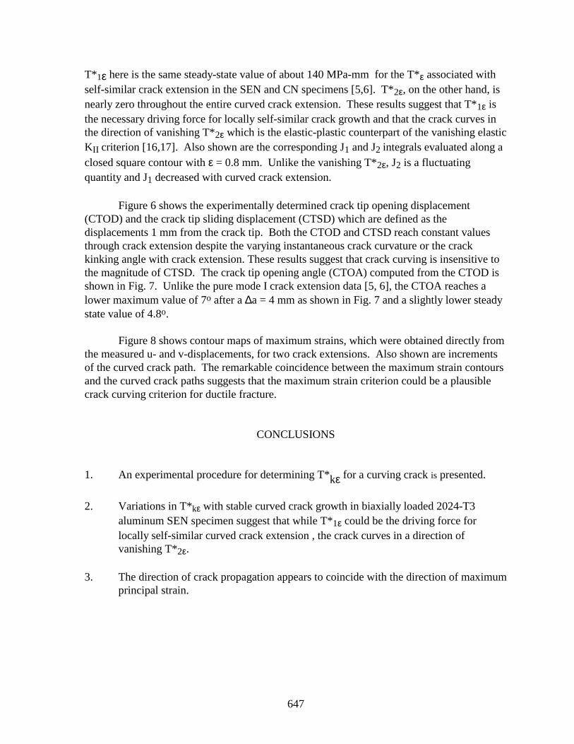
647
T*1ε here is the same steady-state value of about 140 MPa-mm for the T*ε associated withself-similar crack extension in the SEN and CN specimens [5,6]. T*2ε, on the other hand, isnearly zero throughout the entire curved crack extension. These results suggest that T*1ε isthe necessary driving force for locally self-similar crack growth and that the crack curves inthe direction of vanishing T*2ε which is the elastic-plastic counterpart of the vanishing elasticKII criterion [16,17]. Also shown are the corresponding J1 and J2 integrals evaluated along aclosed square contour with ε = 0.8 mm. Unlike the vanishing T*2ε, J2 is a fluctuatingquantity and J1 decreased with curved crack extension.
Figure 6 shows the experimentally determined crack tip opening displacement(CTOD) and the crack tip sliding displacement (CTSD) which are defined as thedisplacements 1 mm from the crack tip. Both the CTOD and CTSD reach constant valuesthrough crack extension despite the varying instantaneous crack curvature or the crackkinking angle with crack extension. These results suggest that crack curving is insensitive tothe magnitude of CTSD. The crack tip opening angle (CTOA) computed from the CTOD isshown in Fig. 7. Unlike the pure mode I crack extension data [5, 6], the CTOA reaches alower maximum value of 7o after a ∆a = 4 mm as shown in Fig. 7 and a slightly lower steadystate value of 4.8o.
Figure 8 shows contour maps of maximum strains, which were obtained directly fromthe measured u- and v-displacements, for two crack extensions. Also shown are incrementsof the curved crack path. The remarkable coincidence between the maximum strain contoursand the curved crack paths suggests that the maximum strain criterion could be a plausiblecrack curving criterion for ductile fracture.
CONCLUSIONS
1. An experimental procedure for determining T*kε for a curving crack is presented.
2. Variations in T*kε with stable curved crack growth in biaxially loaded 2024-T3
aluminum SEN specimen suggest that while T*1ε could be the driving force forlocally self-similar curved crack extension , the crack curves in a direction ofvanishing T*2ε.
3. The direction of crack propagation appears to coincide with the direction of maximum
principal strain.
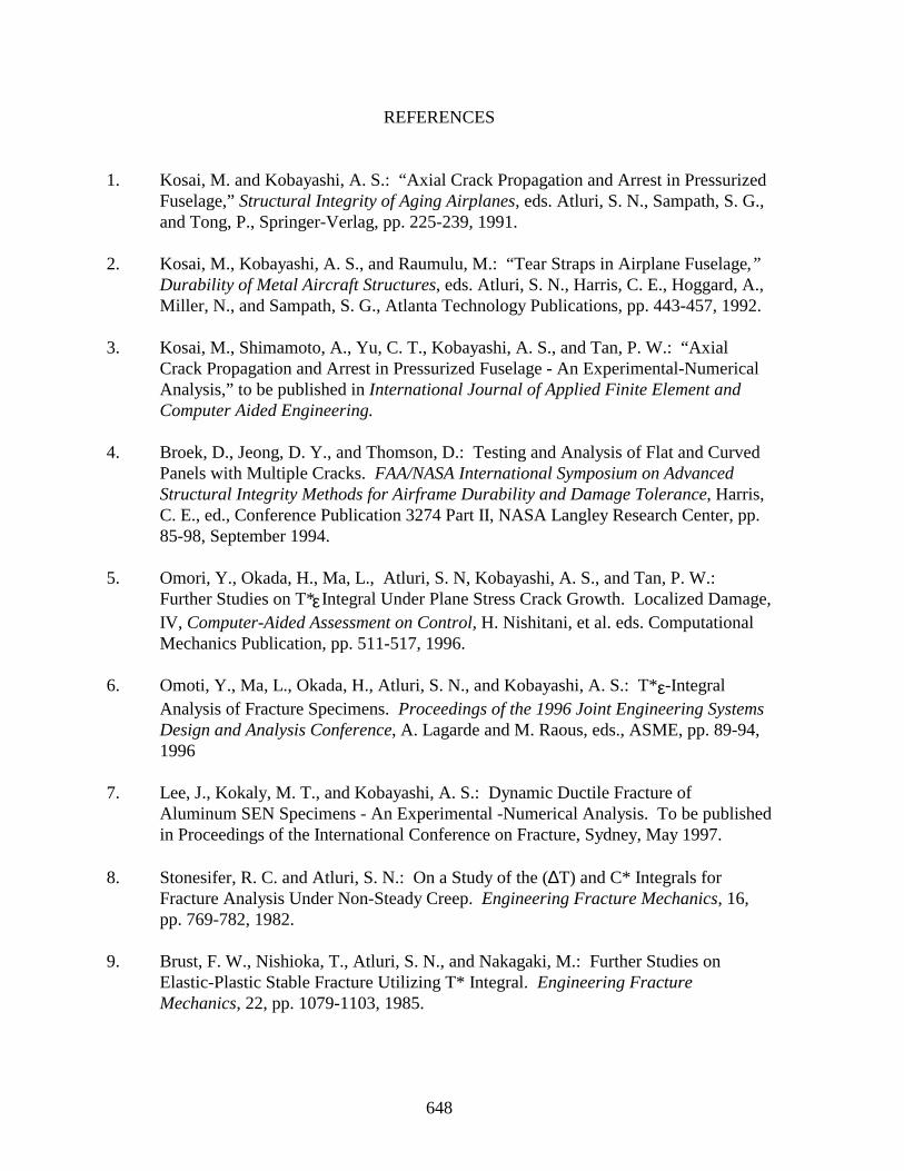
648
REFERENCES
1. Kosai, M. and Kobayashi, A. S.: “Axial Crack Propagation and Arrest in PressurizedFuselage,” Structural Integrity of Aging Airplanes, eds. Atluri, S. N., Sampath, S. G.,and Tong, P., Springer-Verlag, pp. 225-239, 1991.
2. Kosai, M., Kobayashi, A. S., and Raumulu, M.: “Tear Straps in Airplane Fuselage,”
Durability of Metal Aircraft Structures, eds. Atluri, S. N., Harris, C. E., Hoggard, A.,Miller, N., and Sampath, S. G., Atlanta Technology Publications, pp. 443-457, 1992.
3. Kosai, M., Shimamoto, A., Yu, C. T., Kobayashi, A. S., and Tan, P. W.: “Axial
Crack Propagation and Arrest in Pressurized Fuselage - An Experimental-NumericalAnalysis,” to be published in International Journal of Applied Finite Element andComputer Aided Engineering.
4. Broek, D., Jeong, D. Y., and Thomson, D.: Testing and Analysis of Flat and Curved
Panels with Multiple Cracks. FAA/NASA International Symposium on AdvancedStructural Integrity Methods for Airframe Durability and Damage Tolerance, Harris,C. E., ed., Conference Publication 3274 Part II, NASA Langley Research Center, pp.85-98, September 1994.
5. Omori, Y., Okada, H., Ma, L., Atluri, S. N, Kobayashi, A. S., and Tan, P. W.:
Further Studies on T*ε Integral Under Plane Stress Crack Growth. Localized Damage,IV, Computer-Aided Assessment on Control, H. Nishitani, et al. eds. ComputationalMechanics Publication, pp. 511-517, 1996.
6. Omoti, Y., Ma, L., Okada, H., Atluri, S. N., and Kobayashi, A. S.: T*ε-Integral
Analysis of Fracture Specimens. Proceedings of the 1996 Joint Engineering SystemsDesign and Analysis Conference, A. Lagarde and M. Raous, eds., ASME, pp. 89-94,1996
7. Lee, J., Kokaly, M. T., and Kobayashi, A. S.: Dynamic Ductile Fracture of
Aluminum SEN Specimens - An Experimental -Numerical Analysis. To be publishedin Proceedings of the International Conference on Fracture, Sydney, May 1997.
8. Stonesifer, R. C. and Atluri, S. N.: On a Study of the (∆T) and C* Integrals forFracture Analysis Under Non-Steady Creep. Engineering Fracture Mechanics, 16,pp. 769-782, 1982.
9. Brust, F. W., Nishioka, T., Atluri, S. N., and Nakagaki, M.: Further Studies on
Elastic-Plastic Stable Fracture Utilizing T* Integral. Engineering FractureMechanics, 22, pp. 1079-1103, 1985.
649
10. Okada, H. and Atluri, S. N.: T *ε Integral Evaluation From ExperimentalDisplacement Field for a Plate With Stably Propagating Crack: Development ofCalculation Procedure and Implication of T*ε. To be submitted.
11. Narasimhan, R. and Rosaries, A. J.: Three-Dimensional Effects Near a Crack Tip in a
Ductile Three-Point Bend Specimen. ASME Journal of Applied Mechanics, 57, pp.607-617, 1990.
12. Memhard, D., Brock, W., and Fricke, S.: Characterization Ductile Tearing Resistance
by Energy Dissipation Rate. Fatigue, Fracture of Engineering Materials andStrictures, 16, 10, pp. 1109-1124, 1993.
13. Kosai, M., Shimamoto, S., Yu, C.-T., Kobayashi, A. S., and Tan, P. W.: A Biaxial
Test Specimen for Crack Arrest Studies. To be published in ExperimentalMechanics.
14. Ifju, P. and Post, D.: Zero-Thickness Specimen Gratings for Moiré Interferometry.
Experimental Techniques, 15, pp. 45-47, 1991. 15. Wang, F. X., May, G. B., and Kobayashi, A. S.: Low-Spatial Frequency Steep
Geometric Grating for Use in Moiré Interferometry. Optical Engineering, 33, pp.1125-1131, 1994.
16. Cotterell, B. and Rice, J. R.: Slightly Curved or Kinked Cracks. International
Journal of Fracture, 10, pp. 155-169, 1980. 17. Sumi, Y., Nemat-Nasser, S., and Keer, L. M.: On Crack Path Stability in a Finite
Body. Engineering Fracture Mechanics, 22, pp. 759-771, 1985.
650
Figure 1. Curved Crack With a Locally Elongating Path.
Figure 2. Biaxially Loaded SEN Specimen.
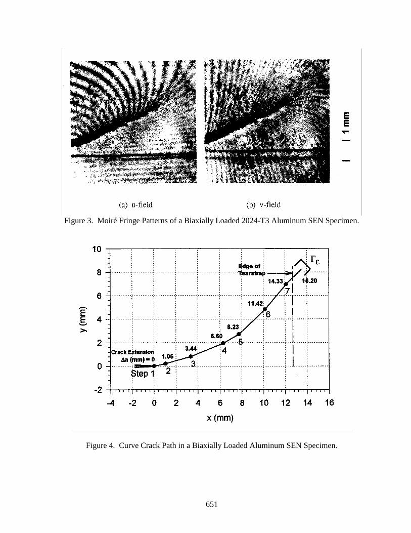
651
Figure 3. Moiré Fringe Patterns of a Biaxially Loaded 2024-T3 Aluminum SEN Specimen.
Figure 4. Curve Crack Path in a Biaxially Loaded Aluminum SEN Specimen.
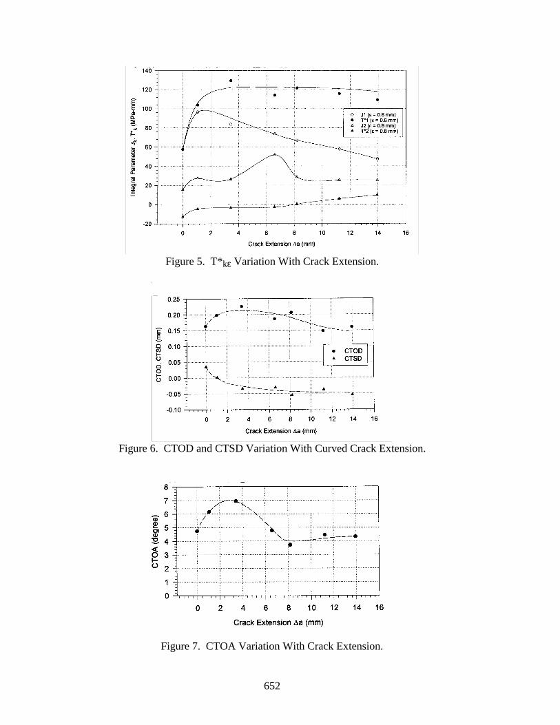
652
Figure 5. T*kε Variation With Crack Extension.
Figure 6. CTOD and CTSD Variation With Curved Crack Extension.
Figure 7. CTOA Variation With Crack Extension.
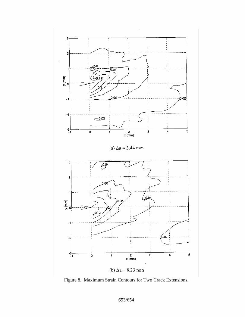
653/654
Figure 8. Maximum Strain Contours for Two Crack Extensions.

655
USE OF NEURAL NETWORKS FORAVIATION SA FETY RISK ASSESSMENT1
Huan-Jyh Shyur, Ph.D. CandidateJames T. Luxhøj, Ph.D.
Department of Industrial EngineeringRutgers University
Trefor P. Williams, Ph.D.Department of Civil Engineering
Rutgers University
SUMMARY
The Event Rate represents the frequency of aviation events (i.e., all accidents,incidents, and occurrences) as reported in the National Program Tracking and ReportingSubsystem (NPTRS). This research focuses on forecasting the number of incidents, alongwith the aggregate Event Rate, with the motivation being that advanced warning andknowledge of the number and trending of potential incidents could lead to enhanced riskassessment and proactive aircraft operator safety measures to prevent serious accidents.
Neural network models are developed to forecast the number of potential incidentsand total Event Rate for aircraft operators with both large and small fleet sizes. Thecontribution of Service Difficulty Reports (SDRs) to the forecasting capability of the neuralnetwork is also examined. The SDR database contains data related to the identification ofabnormal, potentially unsafe conditions in aircraft or aircraft components/equipment.Research results support the use of a Probabilistic Neural Network (PNN) to classify suchinputs as the fleet size, number of SDRs/fleet size, and proportion of unfavorable operationssurveillance inspections into four output classes for the number of potential aircraft incidentsand total events.
INTRODUCTION
The Safety Performance Analysis System (SPAS) is a Federal AviationAdministration (FAA) initiative to develop an integrated decision support system to assistsafety inspectors with surveillance activities (refs. 1, 2). Currently under phase 2
1 This article is based on research performed at Rutgers University. The contents of this paper reflect the viewof the authors who are solely responsible for the accuracy of the facts, analyses, conclusions, andrecommendations presented herein, and do not necessarily reflect the official view or policy of the FederalAviation Administration.
656
development, SPAS is novel to the FAA in that it attempts to integrate safety informationrelated not only to the aircraft, but to aircraft operators, agencies, and personnel. There are anumber of performance measures defined in SPAS for comparing the performance of anyoperator (i.e., airline) to another operator or to national norms with respect to airworthiness,operations, maintenance, equipment, training, reporting, procedures, management, finances,among others (ref. 3).
One of the SPAS performance measures, the Event Rate (ref. 3), represents thefrequency of events (i.e., all accidents, incidents, and occurrences) as recorded in the NationalProgram Tracking and Reporting Subsystem (NPTRS). The calculated value is the totalnumber of these events for a 1-month period divided by the aircraft operator’s fleet size forthat same period. The value is normalized by fleet size to consider that an operator’sexposure to events depends on the number of aircraft in its fleet.
An aircraft accident is defined as an event associated with the operation of an aircraftthat results in death or serious injury and causes substantial damage to the aircraft (ref. 4).An incident is defined as an event, other than an accident, associated with the operation of anaircraft that affects or could affect the safety of operations (ref. 4). For example, near mid-aircollisions, minor damage to an aircraft, and emergency evacuations are classified asincidents. The term occurrence does not have a strict definition, but is used to represent anevent category that is neither an accident nor an incident. As an example, an occurrencecould be an anomalous reading on a gauge that led to the plane taxiing back from the runway.If the anomalous reading could not be reproduced by the maintenance crew, then this eventwould most likely be classified as an occurrence. Although there are guidelines offered toFAA safety inspectors in conducting their investigations, in some cases, the classification ofan event as either an accident, incident, or occurrence is subject to inspector judgment andexperience.
If risk is considered to be exposure to possible loss or injury, then advanced warningand knowledge of the number and trending of potential aircraft incidents could lead toenhanced risk assessment and to proactive operator safety measures to prevent more seriousaccidents. Neural network models are developed to forecast the number of potentialincidents for aircraft operators with both large and small fleet sizes for the next 3-monthperiod. The contribution of the Service Difficulty Reporting (SDR) database that containsdata related to the identification of abnormal, potentially unsafe condition in aircraft oraircraft components and equipment is particularly assessed.
NEURAL NETWORK MODELING
Emanating from research in artificial intelligence (AI) (McCulloch and Pitts (ref. 5));Hopfield (refs. 6, 7), neural network (NN) attempt to simulate the functioning of humanbiological neurons. Neural networks have been particularly useful in pattern recognitionproblems that involve capturing and learning complex underlying (but consistent) trends in
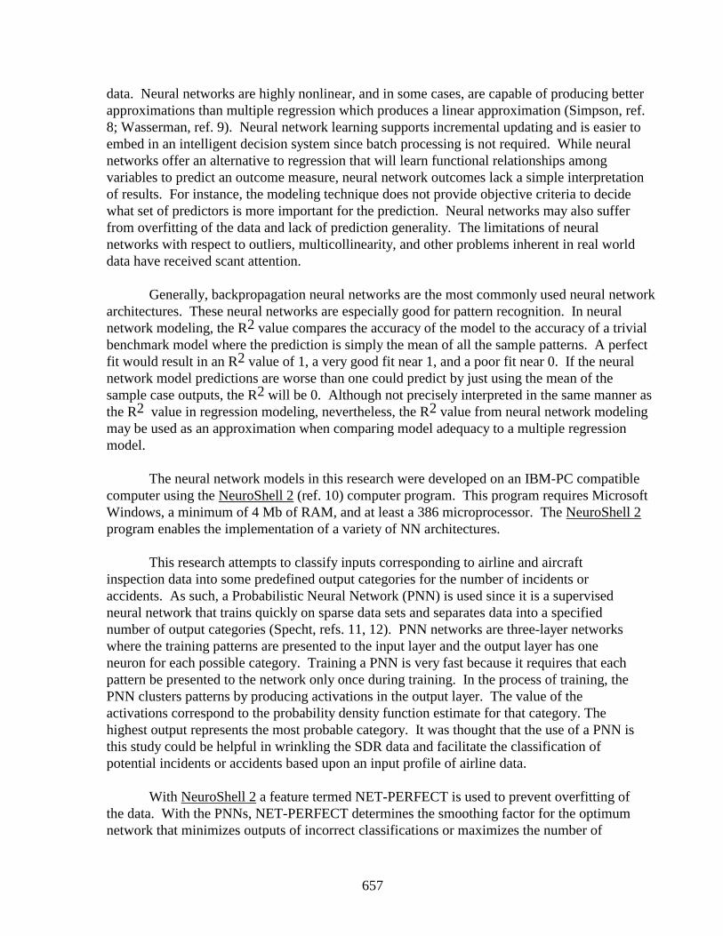
657
data. Neural networks are highly nonlinear, and in some cases, are capable of producing betterapproximations than multiple regression which produces a linear approximation (Simpson, ref.8; Wasserman, ref. 9). Neural network learning supports incremental updating and is easier toembed in an intelligent decision system since batch processing is not required. While neuralnetworks offer an alternative to regression that will learn functional relationships amongvariables to predict an outcome measure, neural network outcomes lack a simple interpretationof results. For instance, the modeling technique does not provide objective criteria to decidewhat set of predictors is more important for the prediction. Neural networks may also sufferfrom overfitting of the data and lack of prediction generality. The limitations of neuralnetworks with respect to outliers, multicollinearity, and other problems inherent in real worlddata have received scant attention.
Generally, backpropagation neural networks are the most commonly used neural networkarchitectures. These neural networks are especially good for pattern recognition. In neuralnetwork modeling, the R2 value compares the accuracy of the model to the accuracy of a trivialbenchmark model where the prediction is simply the mean of all the sample patterns. A perfectfit would result in an R2 value of 1, a very good fit near 1, and a poor fit near 0. If the neuralnetwork model predictions are worse than one could predict by just using the mean of thesample case outputs, the R2 will be 0. Although not precisely interpreted in the same manner asthe R2 value in regression modeling, nevertheless, the R2 value from neural network modelingmay be used as an approximation when comparing model adequacy to a multiple regressionmodel.
The neural network models in this research were developed on an IBM-PC compatiblecomputer using the NeuroShell 2 (ref. 10) computer program. This program requires MicrosoftWindows, a minimum of 4 Mb of RAM, and at least a 386 microprocessor. The NeuroShell 2program enables the implementation of a variety of NN architectures.
This research attempts to classify inputs corresponding to airline and aircraftinspection data into some predefined output categories for the number of incidents oraccidents. As such, a Probabilistic Neural Network (PNN) is used since it is a supervisedneural network that trains quickly on sparse data sets and separates data into a specifiednumber of output categories (Specht, refs. 11, 12). PNN networks are three-layer networkswhere the training patterns are presented to the input layer and the output layer has oneneuron for each possible category. Training a PNN is very fast because it requires that eachpattern be presented to the network only once during training. In the process of training, thePNN clusters patterns by producing activations in the output layer. The value of theactivations correspond to the probability density function estimate for that category. Thehighest output represents the most probable category. It was thought that the use of a PNN isthis study could be helpful in wrinkling the SDR data and facilitate the classification ofpotential incidents or accidents based upon an input profile of airline data.
With NeuroShell 2 a feature termed NET-PERFECT is used to prevent overfitting ofthe data. With the PNNs, NET-PERFECT determines the smoothing factor for the optimumnetwork that minimizes outputs of incorrect classifications or maximizes the number of
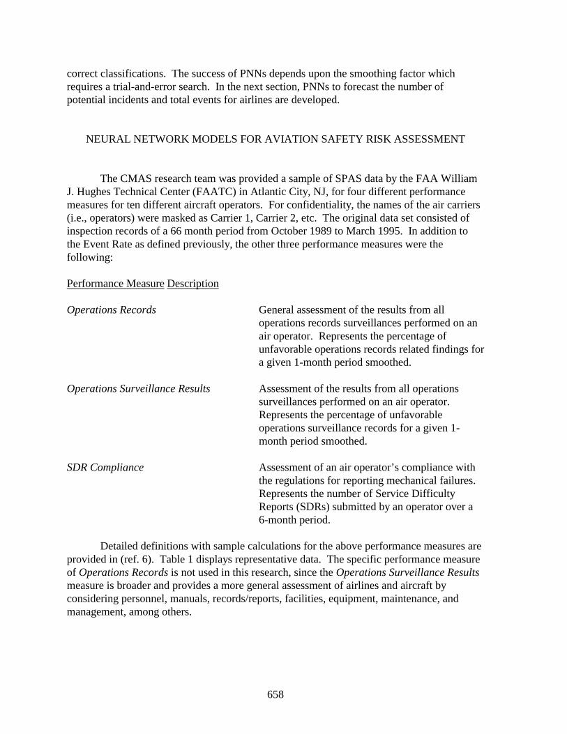
658
correct classifications. The success of PNNs depends upon the smoothing factor whichrequires a trial-and-error search. In the next section, PNNs to forecast the number ofpotential incidents and total events for airlines are developed.
NEURAL NETWORK MODELS FOR AVIATION SAFETY RISK ASSESSMENT
The CMAS research team was provided a sample of SPAS data by the FAA WilliamJ. Hughes Technical Center (FAATC) in Atlantic City, NJ, for four different performancemeasures for ten different aircraft operators. For confidentiality, the names of the air carriers(i.e., operators) were masked as Carrier 1, Carrier 2, etc. The original data set consisted ofinspection records of a 66 month period from October 1989 to March 1995. In addition tothe Event Rate as defined previously, the other three performance measures were thefollowing:
Performance Measure Description
Operations Records General assessment of the results from alloperations records surveillances performed on anair operator. Represents the percentage ofunfavorable operations records related findings fora given 1-month period smoothed.
Operations Surveillance Results Assessment of the results from all operationssurveillances performed on an air operator.Represents the percentage of unfavorableoperations surveillance records for a given 1-month period smoothed.
SDR Compliance Assessment of an air operator’s compliance withthe regulations for reporting mechanical failures.Represents the number of Service DifficultyReports (SDRs) submitted by an operator over a6-month period.
Detailed definitions with sample calculations for the above performance measures areprovided in (ref. 6). Table 1 displays representative data. The specific performance measureof Operations Records is not used in this research, since the Operations Surveillance Resultsmeasure is broader and provides a more general assessment of airlines and aircraft byconsidering personnel, manuals, records/reports, facilities, equipment, maintenance, andmanagement, among others.
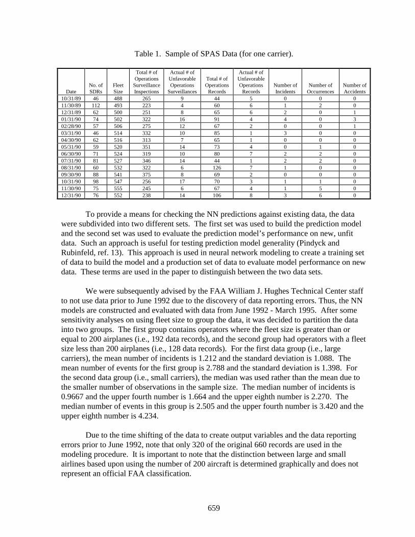
659
Table 1. Sample of SPAS Data (for one carrier).
DateNo. ofSDRs
FleetSize
Total # ofOperations
SurveillanceInspections
Actual # ofUnfavorableOperations
Surveillances
Total # ofOperationsRecords
Actual # ofUnfavorableOperationsRecords
Number ofIncidents
Number ofOccurrences
Number ofAccidents
10/31/89 46 488 265 9 44 5 0 0 011/30/89 112 493 223 4 60 6 1 2 012/31/89 62 500 251 8 65 6 2 0 101/31/90 74 502 322 16 91 4 4 0 302/28/90 57 506 275 12 67 2 0 0 103/31/90 46 514 332 10 85 1 3 0 004/30/90 62 516 313 7 65 1 0 0 005/31/90 59 520 351 14 73 4 0 1 006/30/90 71 524 319 10 80 7 2 2 007/31/90 81 527 346 14 44 1 2 2 008/31/90 60 532 322 6 126 7 1 0 009/30/90 88 541 375 8 69 2 0 0 010/31/90 98 547 256 17 70 3 1 1 011/30/90 75 555 245 6 67 4 1 5 012/31/90 76 552 238 14 106 8 3 6 0
To provide a means for checking the NN predictions against existing data, the datawere subdivided into two different sets. The first set was used to build the prediction modeland the second set was used to evaluate the prediction model’s performance on new, unfitdata. Such an approach is useful for testing prediction model generality (Pindyck andRubinfeld, ref. 13). This approach is used in neural network modeling to create a training setof data to build the model and a production set of data to evaluate model performance on newdata. These terms are used in the paper to distinguish between the two data sets.
We were subsequently advised by the FAA William J. Hughes Technical Center staffto not use data prior to June 1992 due to the discovery of data reporting errors. Thus, the NNmodels are constructed and evaluated with data from June 1992 - March 1995. After somesensitivity analyses on using fleet size to group the data, it was decided to partition the datainto two groups. The first group contains operators where the fleet size is greater than orequal to 200 airplanes (i.e., 192 data records), and the second group had operators with a fleetsize less than 200 airplanes (i.e., 128 data records). For the first data group (i.e., largecarriers), the mean number of incidents is 1.212 and the standard deviation is 1.088. Themean number of events for the first group is 2.788 and the standard deviation is 1.398. Forthe second data group (i.e., small carriers), the median was used rather than the mean due tothe smaller number of observations in the sample size. The median number of incidents is0.9667 and the upper fourth number is 1.664 and the upper eighth number is 2.270. Themedian number of events in this group is 2.505 and the upper fourth number is 3.420 and theupper eighth number is 4.234.
Due to the time shifting of the data to create output variables and the data reportingerrors prior to June 1992, note that only 320 of the original 660 records are used in themodeling procedure. It is important to note that the distinction between large and smallairlines based upon using the number of 200 aircraft is determined graphically and does notrepresent an official FAA classification.
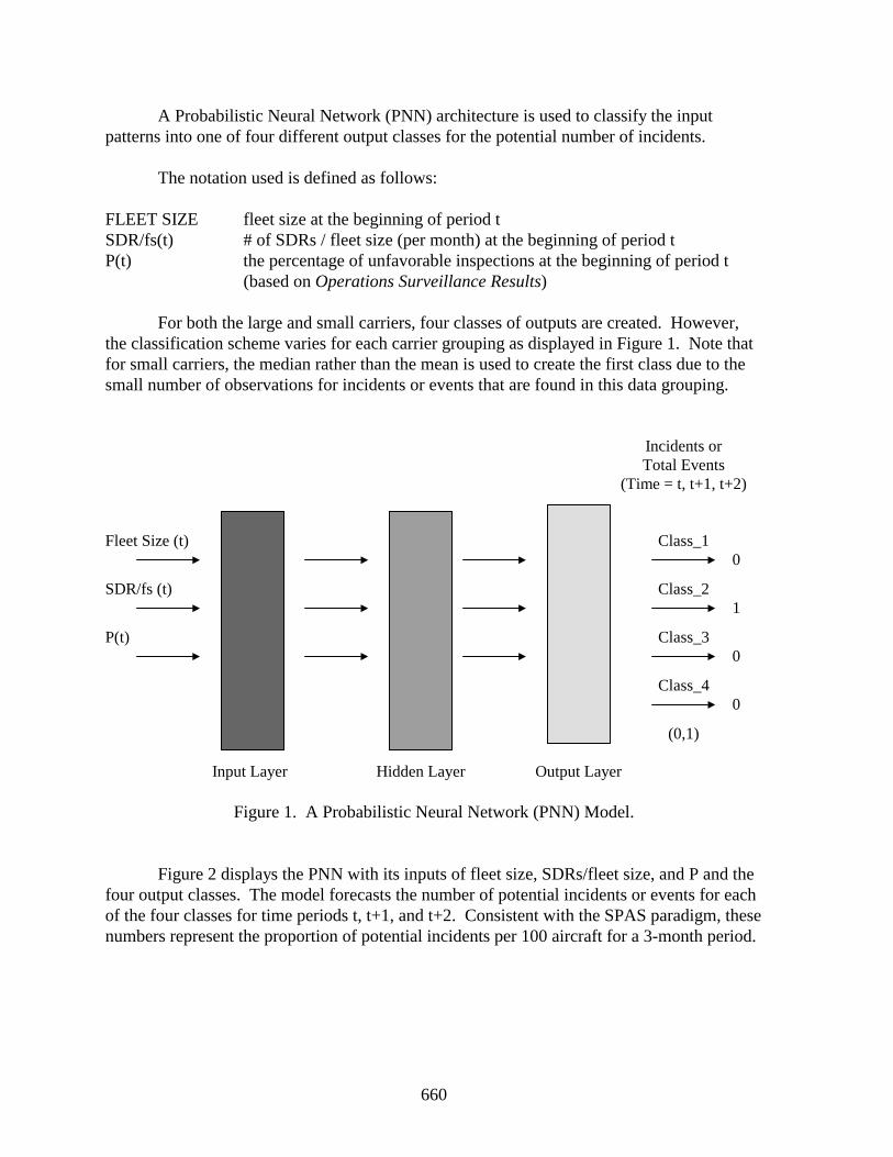
660
A Probabilistic Neural Network (PNN) architecture is used to classify the inputpatterns into one of four different output classes for the potential number of incidents.
The notation used is defined as follows:
FLEET SIZE fleet size at the beginning of period tSDR/fs(t) # of SDRs / fleet size (per month) at the beginning of period tP(t) the percentage of unfavorable inspections at the beginning of period t
(based on Operations Surveillance Results)
For both the large and small carriers, four classes of outputs are created. However,the classification scheme varies for each carrier grouping as displayed in Figure 1. Note thatfor small carriers, the median rather than the mean is used to create the first class due to thesmall number of observations for incidents or events that are found in this data grouping.
Incidents orTotal Events
(Time = t, t+1, t+2)
Fleet Size (t) Class_10
SDR/fs (t) Class_21
P(t) Class_30
Class_40
(0,1)
Input Layer Hidden Layer Output Layer
Figure 1. A Probabilistic Neural Network (PNN) Model.
Figure 2 displays the PNN with its inputs of fleet size, SDRs/fleet size, and P and thefour output classes. The model forecasts the number of potential incidents or events for eachof the four classes for time periods t, t+1, and t+2. Consistent with the SPAS paradigm, thesenumbers represent the proportion of potential incidents per 100 aircraft for a 3-month period.
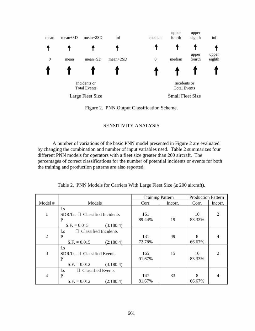
661
mean mean+SD mean+2SD inf medianupperfourth
uppereighth inf
0 mean mean+SD mean+2SD 0 medianupperfourth
uppereighth
Incidents orTotal Events
Incidents orTotal Events
Large Fleet Size Small Fleet Size
Figure 2. PNN Output Classification Scheme.
SENSITIVITY ANALYSIS
A number of variations of the basic PNN model presented in Figure 2 are evaluatedby changing the combination and number of input variables used. Table 2 summarizes fourdifferent PNN models for operators with a fleet size greater than 200 aircraft. Thepercentages of correct classifications for the number of potential incidents or events for boththe training and production patterns are also reported.
Table 2. PNN Models for Carriers With Large Fleet Size (≥ 200 aircraft).
Training Pattern Production PatternModel # Models Corr. Incorr. Corr. Incorr.
1f.sSDR/f.s. ⇒ Classified IncidentsP
S.F. = 0.015 (3:180:4)
16189.44% 19
1083.33%
2
2f.s ⇒ Classified IncidentsP
S.F. = 0.015 (2:180:4)131
72.78%49 8
66.67%4
3f.sSDR/f.s. ⇒ Classified EventsP
S.F. = 0.012 (3:180:4)
16591.67%
15 1083.33%
2
4f.s ⇒ Classified EventsP
S.F. = 0.012 (2:180:4)147
81.67%33 8
66.67%4
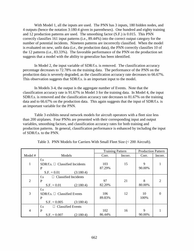
662
With Model 1, all the inputs are used. The PNN has 3 inputs, 180 hidden nodes, and4 outputs (hence the notation 3:180:4 given in parentheses). One hundred and eighty trainingand 12 production patterns are used. The smoothing factor (S.F.) is 0.015. This PNNcorrectly classifies 161 input patterns (i.e., 89.44%) into the correct output category for thenumber of potential incidents. Nineteen patterns are incorrectly classified. When the modelis evaluated on new, unfit data (i.e., the production data), the PNN correctly classifies 10 ofthe 12 patterns (i.e., 83.33%). The favorable performance of the PNN on the production setsuggests that a model with the ability to generalize has been identified.
In Model 2, the input variable of SDR/f.s. is removed. The classification accuracypercentage decreases to 72.78% on the training data. The performance of the PNN on theproduction data is severely degraded, as the classification accuracy rate decreases to 66.67%.This observation suggests that SDR/f.s. is an important input to the model.
In Models 3-4, the output is the aggregate number of Events. Note that theclassification accuracy rate is 91.67% in Model 3 for the training data. In Model 4, the inputSDR/f.s. is removed and the classification accuracy rate decreases to 81.67% on the trainingdata and to 66.67% on the production data. This again suggests that the input of SDR/f.s. isan important variable for the PNN.
Table 3 exhibits neural network models for aircraft operators with a fleet size lessthan 200 airplanes. Four PNNs are presented with their corresponding input and outputvariables, smoothing factors, and classification accuracy rates for both training andproduction patterns. In general, classification performance is enhanced by including the inputof SDR/f.s. to the PNN.
Table 3. PNN Models for Carriers With Small Fleet Size (< 200 Aircraft).
Training Pattern Production PatternModel # Models Corr. Incorr. Corr. Incorr.
1f.sSDR/f.s. ⇒ Classified IncidentsP
S.F. = 0.01 (3:180:4)
10387.29%
15 990.00%
1
2f.s ⇒ Classified IncidentsP
S.F. = 0.01 (2:180:4)97
82.20%21 8
80.00%2
3f.sSDR/f.s. ⇒ Classified EventsP
S.F. = 0.005 (3:180:4)
10689.83%
12 10100%
0
4f.s ⇒ Classified EventsP
S.F. = 0.007 (2:180:4)102
86.44%16 9
90.00%1
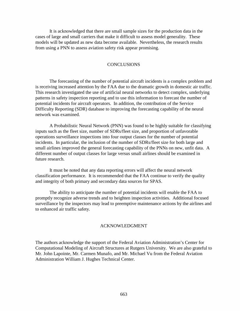
663
It is acknowledged that there are small sample sizes for the production data in thecases of large and small carriers that make it difficult to assess model generality. Thesemodels will be updated as new data become available. Nevertheless, the research resultsfrom using a PNN to assess aviation safety risk appear promising.
CONCLUSIONS
The forecasting of the number of potential aircraft incidents is a complex problem andis receiving increased attention by the FAA due to the dramatic growth in domestic air traffic.This research investigated the use of artificial neural networks to detect complex, underlyingpatterns in safety inspection reporting and to use this information to forecast the number ofpotential incidents for aircraft operators. In addition, the contribution of the ServiceDifficulty Reporting (SDR) database to improving the forecasting capability of the neuralnetwork was examined.
A Probabilistic Neural Network (PNN) was found to be highly suitable for classifyinginputs such as the fleet size, number of SDRs/fleet size, and proportion of unfavorableoperations surveillance inspections into four output classes for the number of potentialincidents. In particular, the inclusion of the number of SDRs/fleet size for both large andsmall airlines improved the general forecasting capability of the PNNs on new, unfit data. Adifferent number of output classes for large versus small airlines should be examined infuture research.
It must be noted that any data reporting errors will affect the neural networkclassification performance. It is recommended that the FAA continue to verify the qualityand integrity of both primary and secondary data sources for SPAS.
The ability to anticipate the number of potential incidents will enable the FAA topromptly recognize adverse trends and to heighten inspection activities. Additional focusedsurveillance by the inspectors may lead to preemptive maintenance actions by the airlines andto enhanced air traffic safety.
ACKNOWLEDGMENT
The authors acknowledge the support of the Federal Aviation Administration’s Center forComputational Modeling of Aircraft Structures at Rutgers University. We are also grateful toMr. John Lapointe, Mr. Carmen Munafo, and Mr. Michael Vu from the Federal AviationAdministration William J. Hughes Technical Center.
664
REFERENCES
1. Safety Performance Analysis Subsystem, “Functional Description Document,” U.S.Department of Transportation, Volpe National Transportation Systems Center,Cambridge, MA, March 1992.
2. Safety Performance Analysis Subsystem, “Prototype Concept Document,” U.S.
Department of Transportation, Volpe National Transportation Systems Center,Cambridge, MA, April 1992.
3. Safety Performance Analysis System, “SPAS Performance Measure Definitions
(Version 1.0),” U.S. Department of Transportation, Volpe National TransportationSystems Center, Cambridge, MA, October 1995.
4. The Federal Aviation Administration Airworthiness Inspector’s Handbook, FAA
Order 8300.10, Volume 2, Department of Transportation, September 1989. 5. McCulloch, W. S. and Pitts, W., “A Logical Calculus of Ideas Immanent in Nervous
Activity,” Bulletin of Mathematical Biophysics, Vol. 5, 1943, pp. 115-133. 6. Hopfield, J. J., “Neurons With Graded Response Have Collective Computational
Properties Like Those of Two-State Neurons,” Proceedings of the National Academyof Science, Vol. 81, 1984, pp. 3088-3092.
7. Hopfield, J. J., “Neural Networks and Physical Systems With Emergent Collective
Abilities,” Proceedings of the National Academy of Science, Vol. 79, 1982, pp. 2554-2558.
8. Simpson, P., Artificial Neural Systems, Pergamon Press, New York, NY, 1990. 9. Wasserman, P., Neural Computing: Theory and Practice, Van Nostrand Reinhold,
New York, NY, 1989. 10. NeuroShell 2, Ward Systems Group, Inc., Frederick, MD, 1993. 11. Specht, D., “Probabilistic Neural Networks for Classification, Mapping, or
Associative Memory,” Proceedings of the IEEE International Conference on NeuralNetworks, Vol. 1, 1988, pp. 525-532.
12. Specht, D., “Probabilistic Neural Networks,” Neural Networks, Vol. 3, 1990, pp. 109-
118. 13. Pindyck, R. S. and Rubinfield, D. L., Econometric Models and Economic Forecasts,
McGraw-Hill, New York, NY, 1991.
665
WIDESPREAD FATIGUE DAMAGE THRESHOLD ESTIMATES
I. C. Whittaker and H. C. ChenBoeing Commercial Airplane Group
Seattle, Washington
ABSTRACT
This paper describes a simple analytical tool for the use by structures engineers topredict the operational age at which a fleet of airplanes would start to experience more thanthe isolated incident of fatigue cracking. This operational age is often referred to as a fatiguethreshold and is usually measured in flights. The analysis approach follows the traditionalpractice used for fatigue design by applying a “reduction-factor” to individual structuralcomponent average life estimate (central tendency fatigue performance) to determine thefatigue threshold. The two-parameter Weibull distribution with assumed shape parameters isused to develop the procedure for use by structures engineers. The procedure is facilitated bya nomograph which is entered with the number of structural components in the population andon exiting the reduction-factor is obtained. The structures engineer must identify certaintargets such as the limits on the number of fatigued components and the number details withinany single component. Several examples of application of this test/service statistics basedmethod to estimation of widespread fatigue damage threshold are provided.
INTRODUCTION
The likelihood of the occurrence of fatigue damage in an airplane structure increaseswith the number of flights the airplane experiences. Commercial airplanes are generallydesigned with an intended minimum design service objective during which the probability offatigue cracking is expected to be low and if cracks do occur they will be in isolation andgrow independently. Airplanes are frequently utilized beyond their original design serviceobjective in the current commercial airline industry. This makes damage tolerant structurestogether with competent fatigue damage inspection programs essential elements to ensurecontinuous airworthiness for aging airplanes throughout their operational lives untileconomics dictate their retirement from service.
Multiple cracks may occur and become interactively dependent as they grow in anaging airplane. Existing damage tolerance programs for aging fleets such as the supplementalstructural inspection program only address damage at multiple sites or elements, whosedamage extent is restricted to a loca l structural area or detail and no significant damage existsbeyond this area. Since the Aloha 737 accident in 1988, much of the focus has been onwidespread fatigue damage (WFD) (Figure 1). WFD has been characterized by the
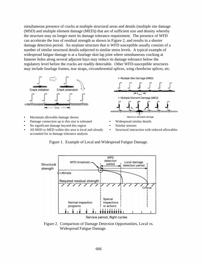
666
simultaneous presence of cracks at multiple structural areas and details (multiple site damage(MSD) and multiple element damage (MED)) that are of sufficient size and density wherebythe structure may no longer meet its damage tolerance requirement. The presence of WFDcan accelerate the loss of residual strength as shown in Figure 2, and results in a shorterdamage detection period. An airplane structure that is WFD susceptible usually consists of anumber of similar structural details subjected to similar stress levels. A typical example ofwidespread fatigue damage is at a fuselage skin lap joint where simultaneous cracking atfastener holes along several adjacent bays may reduce its damage tolerance below theregulatory level before the cracks are readily detectable. Other WFD-susceptible structuresmay include fuselage frames, tear straps, circumferential splices, wing chordwise splices, etc.
• Maximum allowable damage shown• Damage connection up to this size is tolerated• No significant damage beyond this region• All MSD or MED within this area is local and already
accounted for in damage tolerance analysis
• Widespread similar details• Similar stresses• Structural interaction with reduced allowables
Figure 1. Example of Local and Widespread Fatigue Damage.
Figure 2. Comparison of Damage Detection Opportunities, Local vs.Widespread Fatigue Damage.
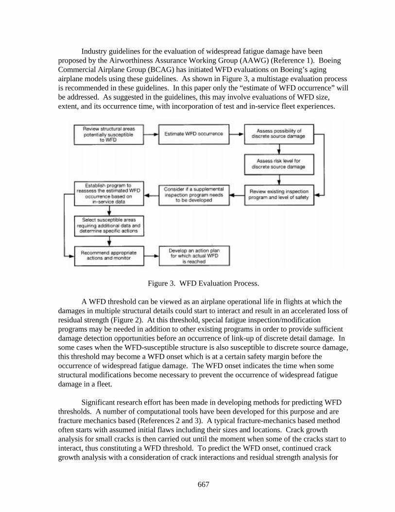
667
Industry guidelines for the evaluation of widespread fatigue damage have beenproposed by the Airworthiness Assurance Working Group (AAWG) (Reference 1). BoeingCommercial Airplane Group (BCAG) has initiated WFD evaluations on Boeing’s agingairplane models using these guidelines. As shown in Figure 3, a multistage evaluation processis recommended in these guidelines. In this paper only the “estimate of WFD occurrence” willbe addressed. As suggested in the guidelines, this may involve evaluations of WFD size,extent, and its occurrence time, with incorporation of test and in-service fleet experiences.
Figure 3. WFD Evaluation Process.
A WFD threshold can be viewed as an airplane operational life in flights at which thedamages in multiple structural details could start to interact and result in an accelerated loss ofresidual strength (Figure 2). At this threshold, special fatigue inspection/modificationprograms may be needed in addition to other existing programs in order to provide sufficientdamage detection opportunities before an occurrence of link-up of discrete detail damage. Insome cases when the WFD-susceptible structure is also susceptible to discrete source damage,this threshold may become a WFD onset which is at a certain safety margin before theoccurrence of widespread fatigue damage. The WFD onset indicates the time when somestructural modifications become necessary to prevent the occurrence of widespread fatiguedamage in a fleet.
Significant research effort has been made in developing methods for predicting WFDthresholds. A number of computational tools have been developed for this purpose and arefracture mechanics based (References 2 and 3). A typical fracture-mechanics based methodoften starts with assumed initial flaws including their sizes and locations. Crack growthanalysis for small cracks is then carried out until the moment when some of the cracks start tointeract, thus constituting a WFD threshold. To predict the WFD onset, continued crackgrowth analysis with a consideration of crack interactions and residual strength analysis for
668
determining the occurrence of widespread fatigue damage is often needed. It should be noted,however, the uncertainties associated with initial flaws, loads, and the stochastic nature ofcrack growth and residual strength can make these methods become unnecessarilycomplicated to achieve meaningful results.
This paper describes a simple analytical tool for use by structures engineers to predictWFD thresholds. It incorporates test and service experiences and simple statistical models insuch a way that all the uncertainties are systematically taken into account and the resultingWFD threshold can be estimated at any reliability level. The analysis approach follows thetraditional practice used for fatigue design by applying a reduction factor to the structure’scentral tendency fatigue performance (average life) to determine the fatigue threshold. In thisapproach the factor is dependent on population (i.e., at-risk fleet) size and the interdependentrelationship between structural components and structural details within the component(s).This relationship was developed from Boeing’s extensive test and airplane service databases.
In the following, BCAG’s experience in widespread fatigue damage from service andtest experiences is described. Emphasis is on the extent of cracking, i.e., number of assumedinitiated small cracks, that determines the criteria for WFD threshold. It is followed by anexplanation of the proposed approach to predicting WFD threshold and the use ofnomographs in carrying out the prediction. Finally, a few examples are discussed to illustratethe application and effectiveness of the approach.
Fleet Service and Test Experience in WFD
For over four decades, the airplane industry has been using full-scale fatigue tests,panel tests, and data from inspections of in-service jet transports to validate the designconcepts and identify appropriate preventive maintenance actions for the fleets. In early years,all the full-scale tests and uses of service data were aimed at validating the fail-safe conceptthat involves only local damage at multiple sites, e.g., a fuselage fail-safe capability for cracksup to one or two bays. Since the late 1980s, BCAG has conducted a series of full-scalefatigue tests and panel tests to address widespread fatigue damage issues. The primary goalwas to investigate the damage extent that might lead to widespread fatigue damage. Adetailed description of these tests and their findings can be found in Reference 4. Morerecently, under an FAA contract BCAG conducted full-scale panel tests to investigate theeffect of MSD in a lap joint on the residual strength of a simulated wide-body fuselage(Reference 5). Also, a full-scale fatigue test of a retired B727 fuselage has just beencompleted. Very detailed cracking information has been recorded and data reduction iscurrently being undertaken for WFD analysis.
Over the years, as more high-time airplanes remain in service more data from in-service airplanes have become available for developing WFD criteria for aging airplanes.Most of the service data have been from the Boeing Significant Item Reporting System(SIRS) to which most discrepancies found by operators were reported. Other service datacame from service bulletins (SB), fleet survey programs in which engineers went out to the
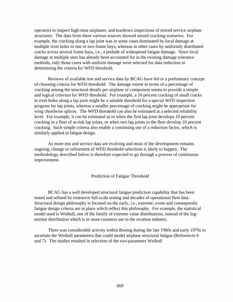
669
operators to inspect high-time airplanes, and teardown inspections of retired service airplanestructures. The data from these various sources showed mixed cracking scenarios. Forexample, the cracking along a lap joint was in some cases dominated by local damage atmultiple rivet holes in one or two frame bays, whereas in other cases by uniformly distributedcracks across several frame bays, i.e., a prelude of widespread fatigue damage. Since localdamage at multiple sites has already been accounted for in the existing damage tolerancemethods, only those cases with uniform damage were selected for data reduction indetermining the criteria for WFD threshold.
Reviews of available test and service data by BCAG have led to a preliminary conceptof choosing criteria for WFD threshold. The damage extent in terms of a percentage ofcracking among the structural details per airplane or component seems to provide a simpleand logical criterion for WFD threshold. For example, a 10 percent cracking of small cracksin rivet holes along a lap joint might be a suitable threshold for a special WFD inspectionprogram for lap joints, whereas a smaller percentage of cracking might be appropriate forwing chordwise splices. The WFD threshold can also be estimated at a selected reliabilitylevel. For example, it can be estimated as to when the first lap joint develops 10 percentcracking in a fleet of at-risk lap joints, or when two lap joints in the fleet develop 10 percentcracking. Such simple criteria also enable a continuing use of a reduction factor, which issimilarly applied in fatigue design.
As more test and service data are evolving and most of the development remainsongoing, change or refinement of WFD threshold selections is likely to happen. Themethodology described below is therefore expected to go through a process of continuousimprovement.
Prediction of Fatigue Threshold
BCAG has a well developed structural fatigue prediction capability that has beentested and refined by extensive full-scale testing and decades of operational fleet data.Structural design philosophy is focused on the early, i.e., extreme, event and consequentlyfatigue design criteria are in place which reflect this philosophy. For example, the statisticalmodel used is Weibull, one of the family of extreme value distributions, instead of the log-normal distribution which is in more common use in the aviation industry.
There was considerable activity within Boeing during the late 1960s and early 1970s toascertain the Weibull parameters that could model airplane structural fatigue (References 6and 7). The studies resulted in selection of the two-parameter Weibull
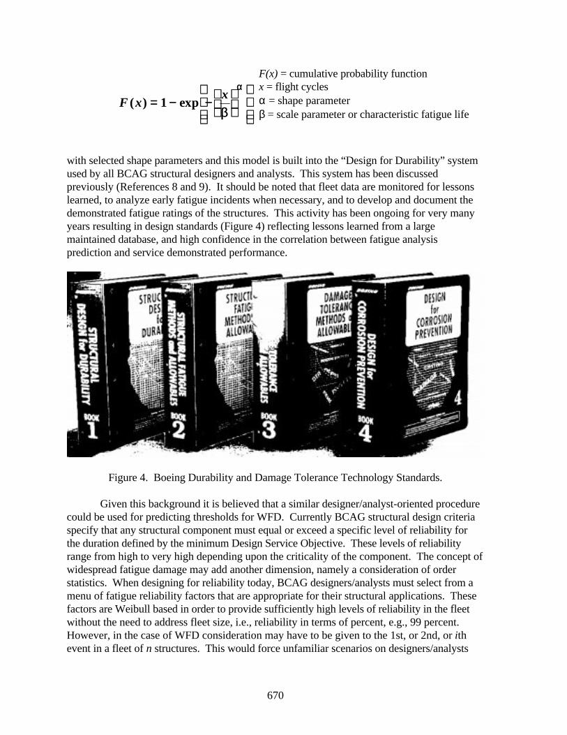
670
F xx
( ) exp== −− −−
1ββ
ααF(x) = cumulative probability functionx = flight cyclesα = shape parameterβ = scale parameter or characteristic fatigue life
with selected shape parameters and this model is built into the “Design for Durability” systemused by all BCAG structural designers and analysts. This system has been discussedpreviously (References 8 and 9). It should be noted that fleet data are monitored for lessonslearned, to analyze early fatigue incidents when necessary, and to develop and document thedemonstrated fatigue ratings of the structures. This activity has been ongoing for very manyyears resulting in design standards (Figure 4) reflecting lessons learned from a largemaintained database, and high confidence in the correlation between fatigue analysisprediction and service demonstrated performance.
Figure 4. Boeing Durability and Damage Tolerance Technology Standards.
Given this background it is believed that a similar designer/analyst-oriented procedurecould be used for predicting thresholds for WFD. Currently BCAG structural design criteriaspecify that any structural component must equal or exceed a specific level of reliability forthe duration defined by the minimum Design Service Objective. These levels of reliabilityrange from high to very high depending upon the criticality of the component. The concept ofwidespread fatigue damage may add another dimension, namely a consideration of orderstatistics. When designing for reliability today, BCAG designers/analysts must select from amenu of fatigue reliability factors that are appropriate for their structural applications. Thesefactors are Weibull based in order to provide sufficiently high levels of reliability in the fleetwithout the need to address fleet size, i.e., reliability in terms of percent, e.g., 99 percent.However, in the case of WFD consideration may have to be given to the 1st, or 2nd, or ithevent in a fleet of n structures. This would force unfamiliar scenarios on designers/analysts
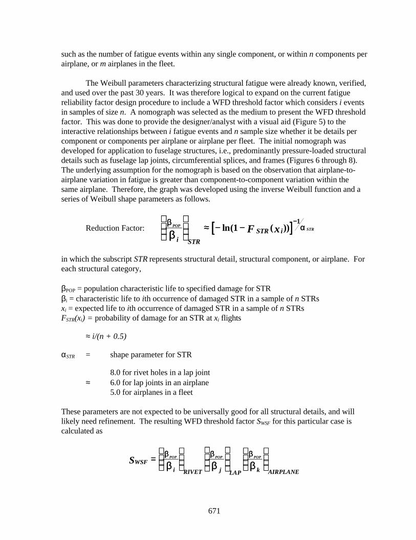
671
such as the number of fatigue events within any single component, or within n components perairplane, or m airplanes in the fleet.
The Weibull parameters characterizing structural fatigue were already known, verified,and used over the past 30 years. It was therefore logical to expand on the current fatiguereliability factor design procedure to include a WFD threshold factor which considers i eventsin samples of size n. A nomograph was selected as the medium to present the WFD thresholdfactor. This was done to provide the designer/analyst with a visual aid (Figure 5) to theinteractive relationships between i fatigue events and n sample size whether it be details percomponent or components per airplane or airplane per fleet. The initial nomograph wasdeveloped for application to fuselage structures, i.e., predominantly pressure-loaded structuraldetails such as fuselage lap joints, circumferential splices, and frames (Figures 6 through 8).The underlying assumption for the nomograph is based on the observation that airplane-to-airplane variation in fatigue is greater than component-to-component variation within thesame airplane. Therefore, the graph was developed using the inverse Weibull function and aseries of Weibull shape parameters as follows.
Reduction Factor: [[ ]]POPSTR
i STR
STR iF xββ ααββ
≈≈ −− −−
−−ln( ( ))1
1
in which the subscript STR represents structural detail, structural component, or airplane. Foreach structural category,
βPOP = population characteristic life to specified damage for STRβi = characteristic life to ith occurrence of damaged STR in a sample of n STRsxi = expected life to ith occurrence of damaged STR in a sample of n STRsFSTR(xi) = probability of damage for an STR at xi flights
≈ i/(n + 0.5)
αSTR = shape parameter for STR
8.0 for rivet holes in a lap joint≈ 6.0 for lap joints in an airplane
5.0 for airplanes in a fleet
These parameters are not expected to be universally good for all structural details, and willlikely need refinement. The resulting WFD threshold factor SWSF for this particular case iscalculated as
WSFi RIVET j LAP k AIRPLANE
S POP POP POP==
ββ ββ ββ
ββ ββ ββ
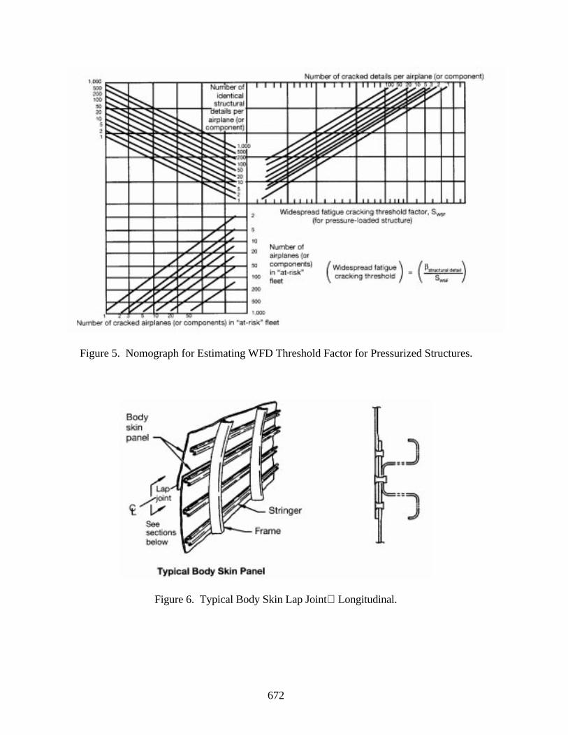
672
Figure 5. Nomograph for Estimating WFD Threshold Factor for Pressurized Structures.
Figure 6. Typical Body Skin Lap JointLongitudinal.
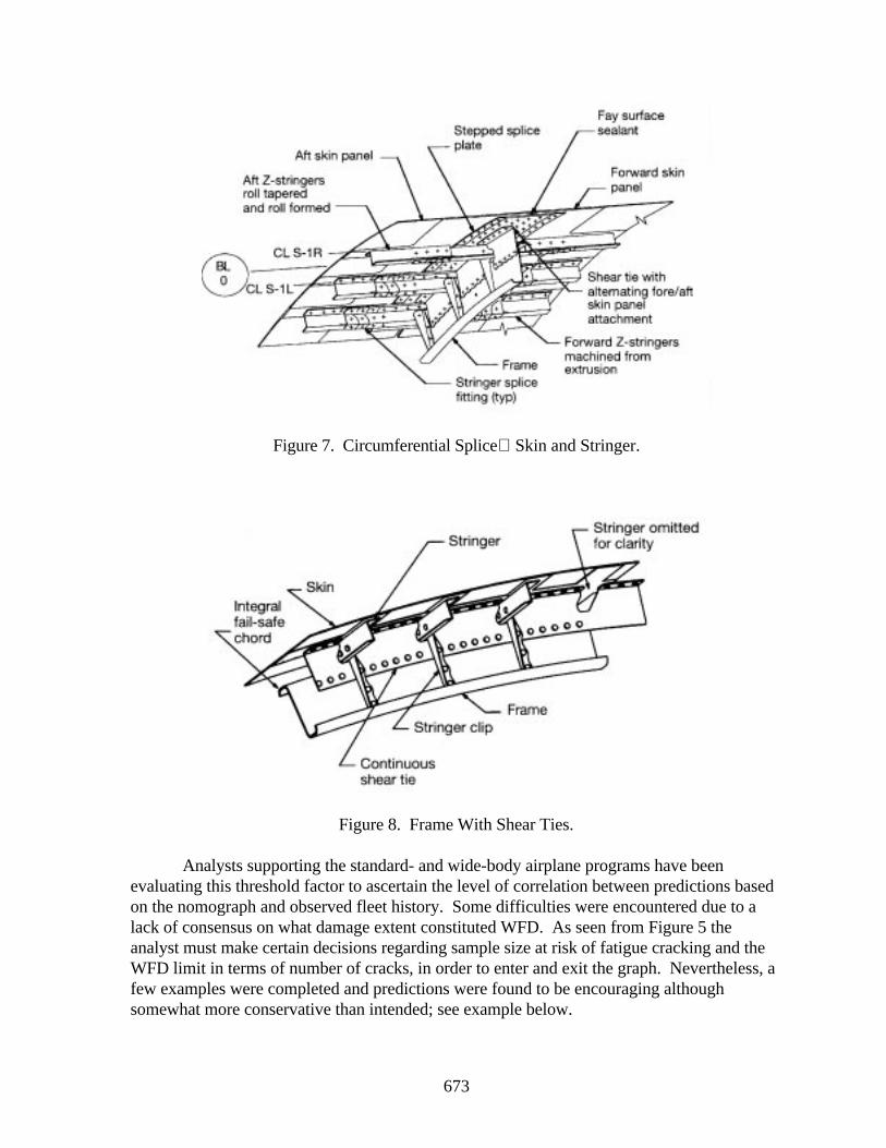
673
Figure 7. Circumferential SpliceSkin and Stringer.
Figure 8. Frame With Shear Ties.
Analysts supporting the standard- and wide-body airplane programs have beenevaluating this threshold factor to ascertain the level of correlation between predictions basedon the nomograph and observed fleet history. Some difficulties were encountered due to alack of consensus on what damage extent constituted WFD. As seen from Figure 5 theanalyst must make certain decisions regarding sample size at risk of fatigue cracking and theWFD limit in terms of number of cracks, in order to enter and exit the graph. Nevertheless, afew examples were completed and predictions were found to be encouraging althoughsomewhat more conservative than intended; see example below.
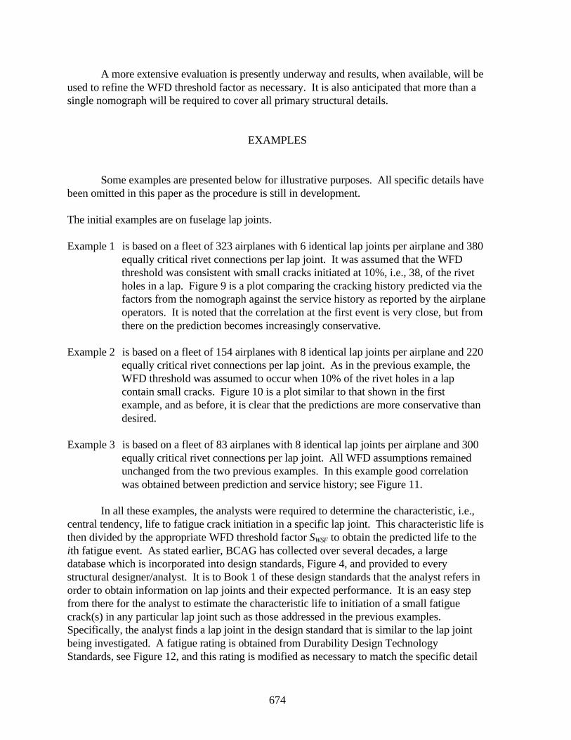
674
A more extensive evaluation is presently underway and results, when available, will beused to refine the WFD threshold factor as necessary. It is also anticipated that more than asingle nomograph will be required to cover all primary structural details.
EXAMPLES
Some examples are presented below for illustrative purposes. All specific details havebeen omitted in this paper as the procedure is still in development.
The initial examples are on fuselage lap joints.
Example 1 is based on a fleet of 323 airplanes with 6 identical lap joints per airplane and 380equally critical rivet connections per lap joint. It was assumed that the WFDthreshold was consistent with small cracks initiated at 10%, i.e., 38, of the rivetholes in a lap. Figure 9 is a plot comparing the cracking history predicted via thefactors from the nomograph against the service history as reported by the airplaneoperators. It is noted that the correlation at the first event is very close, but fromthere on the prediction becomes increasingly conservative.
Example 2 is based on a fleet of 154 airplanes with 8 identical lap joints per airplane and 220equally critical rivet connections per lap joint. As in the previous example, theWFD threshold was assumed to occur when 10% of the rivet holes in a lapcontain small cracks. Figure 10 is a plot similar to that shown in the firstexample, and as before, it is clear that the predictions are more conservative thandesired.
Example 3 is based on a fleet of 83 airplanes with 8 identical lap joints per airplane and 300equally critical rivet connections per lap joint. All WFD assumptions remainedunchanged from the two previous examples. In this example good correlationwas obtained between prediction and service history; see Figure 11.
In all these examples, the analysts were required to determine the characteristic, i.e.,central tendency, life to fatigue crack initiation in a specific lap joint. This characteristic life isthen divided by the appropriate WFD threshold factor SWSF to obtain the predicted life to theith fatigue event. As stated earlier, BCAG has collected over several decades, a largedatabase which is incorporated into design standards, Figure 4, and provided to everystructural designer/analyst. It is to Book 1 of these design standards that the analyst refers inorder to obtain information on lap joints and their expected performance. It is an easy stepfrom there for the analyst to estimate the characteristic life to initiation of a small fatiguecrack(s) in any particular lap joint such as those addressed in the previous examples.Specifically, the analyst finds a lap joint in the design standard that is similar to the lap jointbeing investigated. A fatigue rating is obtained from Durability Design TechnologyStandards, see Figure 12, and this rating is modified as necessary to match the specific detail
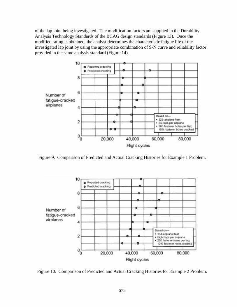
675
of the lap joint being investigated. The modification factors are supplied in the DurabilityAnalysis Technology Standards of the BCAG design standards (Figure 13). Once themodified rating is obtained, the analyst determines the characteristic fatigue life of theinvestigated lap joint by using the appropriate combination of S-N curve and reliability factorprovided in the same analysis standard (Figure 14).
Figure 9. Comparison of Predicted and Actual Cracking Histories for Example 1 Problem.
Figure 10. Comparison of Predicted and Actual Cracking Histories for Example 2 Problem.
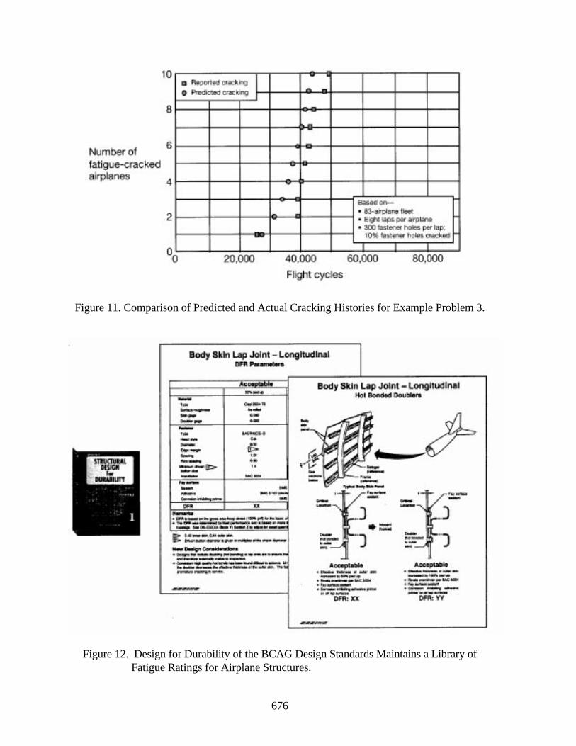
676
Figure 11. Comparison of Predicted and Actual Cracking Histories for Example Problem 3.
Figure 12. Design for Durability of the BCAG Design Standards Maintains a Library ofFatigue Ratings for Airplane Structures.
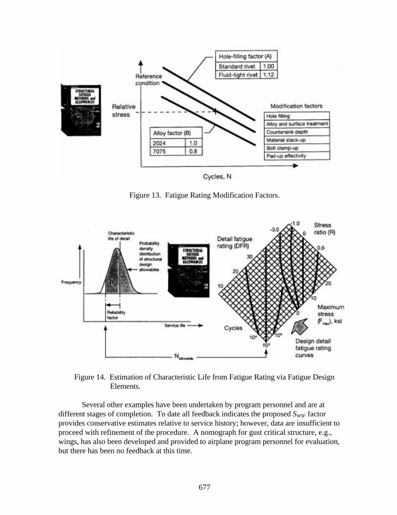
677
Figure 13. Fatigue Rating Modification Factors.
Figure 14. Estimation of Characteristic Life from Fatigue Rating via Fatigue Design Elements.
Several other examples have been undertaken by program personnel and are atdifferent stages of completion. To date all feedback indicates the proposed SWSF factorprovides conservative estimates relative to service history; however, data are insufficient toproceed with refinement of the procedure. A nomograph for gust critical structure, e.g.,wings, has also been developed and provided to airplane program personnel for evaluation,but there has been no feedback at this time.
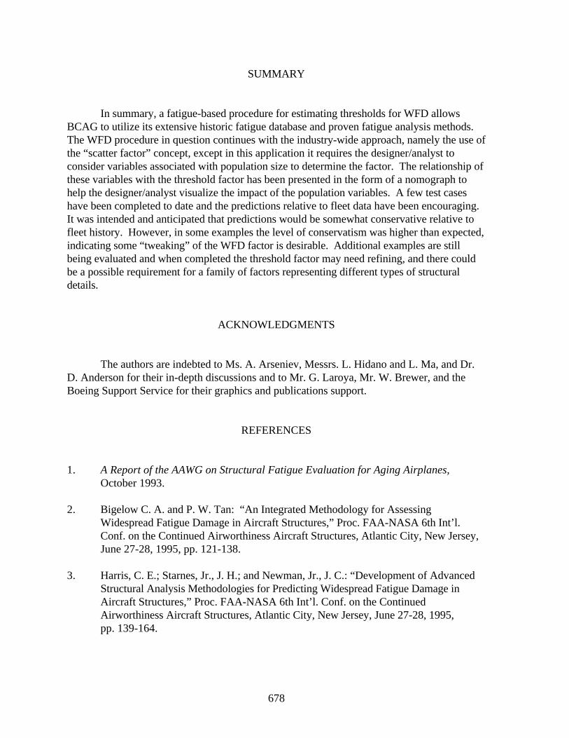
678
SUMMARY
In summary, a fatigue-based procedure for estimating thresholds for WFD allowsBCAG to utilize its extensive historic fatigue database and proven fatigue analysis methods.The WFD procedure in question continues with the industry-wide approach, namely the use ofthe “scatter factor” concept, except in this application it requires the designer/analyst toconsider variables associated with population size to determine the factor. The relationship ofthese variables with the threshold factor has been presented in the form of a nomograph tohelp the designer/analyst visualize the impact of the population variables. A few test caseshave been completed to date and the predictions relative to fleet data have been encouraging.It was intended and anticipated that predictions would be somewhat conservative relative tofleet history. However, in some examples the level of conservatism was higher than expected,indicating some “tweaking” of the WFD factor is desirable. Additional examples are stillbeing evaluated and when completed the threshold factor may need refining, and there couldbe a possible requirement for a family of factors representing different types of structuraldetails.
ACKNOWLEDGMENTS
The authors are indebted to Ms. A. Arseniev, Messrs. L. Hidano and L. Ma, and Dr.D. Anderson for their in-depth discussions and to Mr. G. Laroya, Mr. W. Brewer, and theBoeing Support Service for their graphics and publications support.
REFERENCES
1. A Report of the AAWG on Structural Fatigue Evaluation for Aging Airplanes,October 1993.
2. Bigelow C. A. and P. W. Tan: “An Integrated Methodology for Assessing
Widespread Fatigue Damage in Aircraft Structures,” Proc. FAA-NASA 6th Int’l.Conf. on the Continued Airworthiness Aircraft Structures, Atlantic City, New Jersey,June 27-28, 1995, pp. 121-138.
3. Harris, C. E.; Starnes, Jr., J. H.; and Newman, Jr., J. C.: “Development of Advanced
Structural Analysis Methodologies for Predicting Widespread Fatigue Damage inAircraft Structures,” Proc. FAA-NASA 6th Int’l. Conf. on the ContinuedAirworthiness Aircraft Structures, Atlantic City, New Jersey, June 27-28, 1995,pp. 139-164.

679/680
4. Maclin, J. R.: “Performance of Fuselage Pressure Structure,” 3rd Int’l. Conf. onAging Aircraft and Structural Airworthiness, Washington, DC, November 19-21,1991.
5. Gruber, M. L.; Mazur, C. J.; Wilkins, K. E.; and Worden, R. E.: “Investigation of
Fuselage Structure Subject to Widespread Fatigue Damage,” FAA Technical Report,DOT/FAA/AR-95/47, February 1996.
6. Whittaker, I. C. and Besuner, P. M.: “A Reliability Analysis Approach to Fatigue Life
Variability of Aircraft Structures,” Air Force Materials Laboratory Technical ReportAFML-TR-69-65, April 1969.
7. Whittaker, I. C.: “Development of Titanium and Steel Fatigue Variability Model for
Application of Reliability Analysis Approach to Aircraft Structures,” Air ForceMaterials Laboratory Technical Report AFML-TR-72-236, October 1972.
8. Goranson, U. G.; Hall, J.; Maclin, J. R.; Watanabe, R. T.: “Long Life Damage
Tolerant Jet Transport Structures,” ASTM Symposium on Design of Fatigue andFracture Resistant Structures, November 10-11, 1980.
9. Whittaker, I. C.; Miller, M.; Goranson, U. G.: “Durability and Damage Tolerance
Evaluations of Jet Transport Structures,” Proc. 5th Int’l. Conf. on Structural Safetyand Reliability (ICOSSAR), August 7-11, 1989.