Nanoscale Phenomena in Ultrathin Catalyst Layers of

PEM Fuel Cells: Insights from Molecular Dynamics

by

Amin Nouri Khorasani

B.Sc., Sharif University of Technology, 2010

Thesis Submitted in Partial Fulfillment of the

Requirements for the Degree of

Master of Science

in the

Department of Chemistry

Faculty of Science

Amin Nouri Khorasani 2013

SIMON FRASER UNIVERSITY

Summer 2013

ii

Approval

Name: Amin Nouri Khorasani

Degree: Master of Science

Title of Thesis: Nanoscale Phenomena in Ultrathin Catalyst Layer of

PEM Fuel Cells: Insights from Molecular Dynamics

Examining Committee: Chair: Krzystof Starosta

Associate Professor

Michael H. Eikerling

Senior Supervisor

Professor

Kourosh Malek

Co-supervisor

Adjunct Professor

Gary W. Leach

Supervisor

Associate Professor

Byron D. Gates

Supervisor

Associate Professor

Noham Weinberg

Internal Examiner

Adjunct Professor

Department of Chemistry

Date Defended: May 09, 2013

iii

Partial Copyright Licence

iv

Abstract

Ionomer-free ultrathin catalyst layers have shown promise to enhance the

performance and reduce the platinum loading of catalyst layers in polymer

electrolyte fuel cell. The nanostructure of a catalyst layer affects the distribution

and diffusion of reactants, and consequently its effectiveness factor. We

employed classical molecular dynamics to simulate a catalyst layer pore as a

water-filled channel with faceted walls, and investigated the effect of channel

geometry and charging on hydronium ion and water distribution and diffusion

in the channel.

Equilibrium hydronium ion distribution profiles on the catalyst channel were

obtained to calculate the effect of channel structure on the electrostatic

effectiveness factor of the channel. Furthermore, we calculated the self-diffusion

coefficient and interfacial water structure in the model channel. Results on

proton concentration, diffusion and kinetics are discussed in view of catalyst

layer performance.

Keywords: polymer electrolyte fuel cells; molecular modeling; electrostatic

effects; local reaction conditions; catalyst layer effectiveness

v

Dedication

Dedicated to my dear parents,

Dr. Fahimeh Fatemi, and Dr. Saied Nouri;

all I have and will accomplish

is only due to their love and sacrifice.

vi

Acknowledgements

Firstly, I would like to sincerely thank my senior supervisor, Professor Michael

Eikerling, for giving me the chance to conduct research under his supervision.

His extensive knowledge and expertise in electrochemistry always assured me of

stepping in the right path. His continuous support, encouragement, and patience

helped me obtain a solid knowledge in electrochemistry. He taught me how to

think logically, read critically, research productively and analyze the results

diligently.

I would like to thank my co-supervisor, Dr. Kourosh Malek, for his great help

and support. He patiently taught me high level molecular dynamics technique

from scratch, machine-level programming language and Linux. He kindly

monitored my progress on a day-to-day basis, discussed my results with me and

supported me with precise advice.

I extend my thanks to my supervisory committee members, Dr. Gary Leach and

Dr. Byron Gates, for the high level discussions and recommendations during my

committee meetings. Those discussions helped me understand the larger picture

of my research project, and helped me recognize the significance of my model

beyond the fuel cell context.

I must thank all the past and present members of Dr. Eikerling research group,

for the heated discussions in the group meeting. Not only the scientific

discussion during our group meeting nurtured my mind, but also helped me

improve my technical and public presentation skills. I must specially thank Dr.

vii

Liya Wang for teaching Density Functional Theory, Karen Chan for teaching

COMSOL to me, as well as answering my endless questions in electrochemistry,

Dr. Ehsan Sadeghi for great discussions about fuel cells science and engineering,

and Dr. Anatoly Golovnev for patiently explaining and discussing the relevant

physical concepts and suggesting creative ideas about my work.

I must acknowledge the support from NRC-EME staff for facilitating the logistics

of this research, providing resources to run the computationally extensive

simulations and maintaining the computer network.

Finally, I must thank my family for their emotional as well as academic support

during my studies.

viii

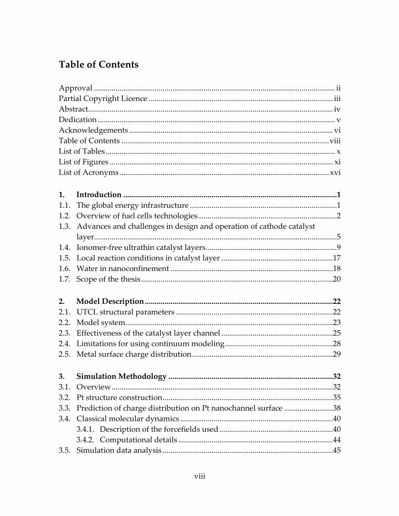
Table of Contents

Approval ........................................................................................................................... ii

Partial Copyright Licence .............................................................................................. iii

Abstract............................................................................................................................. iv

Dedication ......................................................................................................................... v

Acknowledgements ........................................................................................................ vi

Table of Contents .......................................................................................................... viii

List of Tables ..................................................................................................................... x

List of Figures .................................................................................................................. xi

List of Acronyms ........................................................................................................... xvi

1. Introduction .............................................................................................................1

1.1. The global energy infrastructure ...........................................................................1

1.2. Overview of fuel cells technologies .......................................................................2

1.3. Advances and challenges in design and operation of cathode catalyst

layer............................................................................................................................5

1.4. Ionomer-free ultrathin catalyst layers ...................................................................9

1.5. Local reaction conditions in catalyst layer .........................................................17

1.6. Water in nanoconfinement ...................................................................................18

1.7. Scope of the thesis ..................................................................................................20

2. Model Description ................................................................................................22

2.1. UTCL structural parameters ................................................................................22

2.2. Model system ..........................................................................................................23

2.3. Effectiveness of the catalyst layer channel .........................................................25

2.4. Limitations for using continuum modeling .......................................................28

2.5. Metal surface charge distribution ........................................................................29

3. Simulation Methodology ....................................................................................32

3.1. Overview .................................................................................................................32

3.2. Pt structure construction .......................................................................................35

3.3. Prediction of charge distribution on Pt nanochannel surface .........................38

3.4. Classical molecular dynamics ..............................................................................40

3.4.1. Description of the forcefields used ..........................................................40

3.4.2. Computational details ...............................................................................44

3.5. Simulation data analysis .......................................................................................45

ix

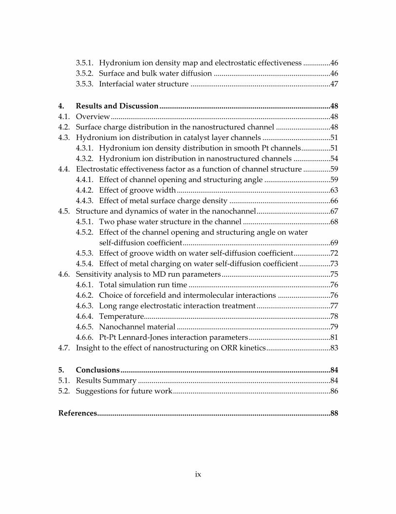
3.5.1. Hydronium ion density map and electrostatic effectiveness ..............46

3.5.2. Surface and bulk water diffusion ............................................................46

3.5.3. Interfacial water structure ........................................................................47

4. Results and Discussion ........................................................................................48

4.1. Overview .................................................................................................................48

4.2. Surface charge distribution in the nanostructured channel ............................48

4.3. Hydronium ion distribution in catalyst layer channels ...................................51

4.3.1. Hydronium ion density distribution in smooth Pt channels ...............51

4.3.2. Hydronium ion distribution in nanostructured channels ...................54

4.4. Electrostatic effectiveness factor as a function of channel structure ..............59

4.4.1. Effect of channel opening and structuring angle ..................................59

4.4.2. Effect of groove width ...............................................................................63

4.4.3. Effect of metal surface charge density ....................................................66

4.5. Structure and dynamics of water in the nanochannel ......................................67

4.5.1. Two phase water structure in the channel .............................................68

4.5.2. Effect of the channel opening and structuring angle on water

self-diffusion coefficient ............................................................................69

4.5.3. Effect of groove width on water self-diffusion coefficient ...................72

4.5.4. Effect of metal charging on water self-diffusion coefficient ................73

4.6. Sensitivity analysis to MD run parameters ........................................................75

4.6.1. Total simulation run time .........................................................................76

4.6.2. Choice of forcefield and intermolecular interactions ...........................76

4.6.3. Long range electrostatic interaction treatment ......................................77

4.6.4. Temperature................................................................................................78

4.6.5. Nanochannel material ...............................................................................79

4.6.6. Pt-Pt Lennard-Jones interaction parameters ..........................................81

4.7. Insight to the effect of nanostructuring on ORR kinetics .................................83

5. Conclusions ............................................................................................................84

5.1. Results Summary ...................................................................................................84

5.2. Suggestions for future work .................................................................................86

References ........................................................................................................................88

x

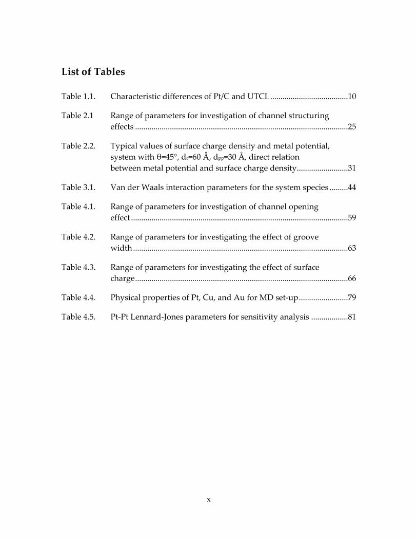
List of Tables

Table 1.1. Characteristic differences of Pt/C and UTCL ......................................10

Table 2.1 Range of parameters for investigation of channel structuring

effects ........................................................................................................25

Table 2.2. Typical values of surface charge density and metal potential,

system with θ=45°, dc=60 Å, dpp=30 Å, direct relation

between metal potential and surface charge density.........................31

Table 3.1. Van der Waals interaction parameters for the system species .........44

Table 4.1. Range of parameters for investigation of channel opening

effect ..........................................................................................................59

Table 4.2. Range of parameters for investigating the effect of groove

width .........................................................................................................63

Table 4.3. Range of parameters for investigating the effect of surface

charge ........................................................................................................66

Table 4.4. Physical properties of Pt, Cu, and Au for MD set-up ........................79

Table 4.5. Pt-Pt Lennard-Jones parameters for sensitivity analysis ..................81

xi

List of Figures

Figure 1.1. Basic design of PEM fuel cell; hydrogen oxidation reaction

occurs in the anode and oxygen reduction reaction in the

cathode. Protons transport through the PEM, and electrons

through the outer electric circuit. ...........................................................4

Figure 1.2. Schematic cross section of a single fuel cell, adapted from

Ref [2] (not to scale). Current conduction between the cells is

through the bipolar plates; flow fields feed fuel/air to the

cell, and GDL influences the transport of gases and liquid

to/from the cell. ..........................................................................................5

Figure 1.3. TEM image of a)Pt/C catalyst, b)PtCo/C alloy catalyst [16],

random dispersion of Pt particles on the substrate; Reprinted

with permission from Elsevier ................................................................7

Figure 1.4. SEM images of: a)Pt/C electrode, b) UTCL with 3M NSTF

design, c) Magnified view of NSTF [43], ionomer-free nature

of the UTCL makes the performance depend on the local

reaction conditions on the CL. Reproduced by the

permission of the Electrochemical Society ..........................................10

Figure 1.5. a) SEM image of NPG. b) High resolution TEM image of

NPG. c) TEM of Pt-coated NPG UTCL at a loading of 0.05

mg.cm-2. d) High resolution TEM of Pt-coated NPG, image

from Ref. [44], Reproduced by the permission of the

Electrochemical Society ..........................................................................11

Figure 1.6. SEM image of Ni75Pt25 nanoparticle for UTCL fabrication,

Ni(II) acetylaacetonate concentration in fabrication process:

A) 0.1, B)0.2, C)0.3, D)0.5 M, Reprinted with permission from

[45], Copyright (2013) American Chemical Society ...........................12

Figure 1.7. SEM image of 3M NSTF electrode a) Catalyst coated

membrane (CCM). b) Zoomed view of a microstructured

catalyst transfer substrate (MCTS) peak. c)Zoomed view of

catalyst electrodes. d) Lower catalyst loading, reprinted from

Ref. [47] with permission from the Electrochemical Society ............14

xii

Figure 1.8. SEM and STEM images of CL whiskerettes, nanostructuring

of whiskerettes shown in e and f. Reprinted from Ref. [47],

with permission from the Electrochemical Society ............................14

Figure 1.9. Schematic illustration of Chan and Eikerling continuum-type

pore-scale model system [51] ................................................................16

Figure 2.1. Electrostatic effectiveness vs potential for different pore

radii. Inset: corresponding surface charge density vs

potential, image from Ref. [51], reproduced by the

permission of the Electrochemical Society. .........................................23

Figure 2.2. Model system schematics, three geometric parameters (θ,dc,

dpp) and metal potential(φM) determine the system ...........................24

Figure 3.1. Overall scheme of the calculations .......................................................34

Figure 3.2. Primitive cell of Pt crystal with FCC structure ..................................35

Figure 3.3. Full atomistic Pt channel structure, incompletely constructed

to better illustrate build-up procedure (left), schematic

representation (right). Water and hydronium ions would be

added to the space in the middle of the structured channel. ...........36

Figure 3.4. 2-d Schematic picture of the model system with physical

boundary conditions ...............................................................................36

Figure 3.5. Force calculation scheme .......................................................................42

Figure 3.6. Radial distribution functions: a)SPC/E, b) SPC (modified), c)

TIP3P (modified)solid line, and the experimental data

dotted. Curves are shifted 2 units for clarity [86]. Reprinted

with permission from the American Chemical Society. ....................43

Figure 4.1. Typical distribution maps in the nanochannel predicted by

PB theory: a) potential distribution, b) proton concentration,

c) Electric field contour lines, d) metal surface charge density ........49

Figure 4.2. Effect of ɸM on the surface charge distribution...................................50

xiii

Figure 4.3. Effect of θ on surface charge distribution, constant dc=20 Å,

dpp=30 Å and ɸM=-50 mV for all cases ...................................................50

Figure 4.4. Pt structured channel with θ=15°, predicted charge

distribution close to homogeneity ........................................................51

Figure 4.5. Schematic of analytically solved electrostatic model system ...........52

Figure 4.6. Wall position definition for PB theory, the wall position is

not defined precisely in an MD simulation; however the

positions of all atoms nuclei are known. .............................................53

Figure 4.8. Hydronium density map (left) and nanostructured channel

(right). The structure is rotated to better represent the

stepped surface, θ=60°, dc=20 Å, dpp=40 Å, and φM=-50 mV. .............55

Figure 4.9. (a) Distribution map of hydronium ions in the nanochannel,

(b) surface hydronium ion density profile, (c) surface

potential, (d) local effectiveness. Dashed lines on the top left

figure indicate the region considered as surface. Channel

with θ=45°, dc=20 Å, dpp=40 Å, φM=-50 mV .......................................56

Figure 4.10. (a) Distribution map of hydronium ions in the nanochannel,

(b) surface hydronium ion density profile, (c) surface

potential, (d) local effectiveness. Dashed lines on the top left

figure indicate the region considered as surface. Channel

with θ=75°, dc=20 Å, dpp=30 Å, and φM=-50 mV ..................................57

Figure 4.11. Relative H3O+ density at channel peak region vs. dc, effect of

walls electrostatic repulsion on H3O+ depletion from peak

region, with constant θ=45°, dpp=30 Å, and φM=-50 mV ....................58

Figure 4.12. Effect of dc on electrostatic effectiveness, Γ; constant dpp=30 Å ........60

Figure 4.13. Direct effect of overall H3O+ concentration on channel

effectiveness, dispersion of data in the low concentration

region is the channel structure-specific effects. ..................................61

xiv

Figure 4.14. Effect of θ on channel effectiveness, Γ, enhanced

effectiveness at smooth surfaces, constant dpp=30 Å, φM=-50

mV. ............................................................................................................62

Figure 4.15. Inverse effect of groove width on electrostatic effectiveness

of nanochannel, constant dc=20 Å .........................................................64

Figure 4.16. Direct effect of overall H3O+ density on Γ, constant dc=20 Å ............65

Figure 4.17. Effect of θ on Γ, constant dc, inverse relation with surface

step fraction..............................................................................................66

Figure 4.18. Direct effect of σM on effectiveness, Γ, due to stronger

Coulomb interaction of H3O+ with walls .............................................67

Figure 4.19. Typical water density map, high contrast of colors indicate a

highly structured phase .........................................................................69

Figure 4.20. Effect of dc on water self-diffusion coefficient, Dw .............................70

Figure 4.21. Analyzing the effect of channel opening on Dw in terms of

ratio of bulk-like (nb) to surface (ns) water ratio .................................71

Figure 4.22. Dependence of Dw to channel structure, a) surface water, b)

bulk-like water .........................................................................................72

Figure 4.23. Effect of groove width on water self-diffusion coefficient, Dw,

dc=20 Å constant. .....................................................................................73

Figure 4.24. Effect of Pt surface charge density on water self-diffusion

coefficient, constant dc=20 Å dpp=30 Å .................................................74

Figure 4.25. Dependence of Dw on Pt surface charge, a) bulk-like water,

b) surface water .......................................................................................75

Figure 4.26. Sensitivity of calculated effectiveness factor to analyzed

trajectory length ......................................................................................76

Figure 4.27 Sensitivity of simulation result and calculation speed to PME

short range force calculation .................................................................78

xv

Figure 4.28. Temperature dependence of channel effectiveness for a

channel with θ=45°, dc=20 Å, dpp=30 Å, σ=-14 μC/cm2 .........................79

Figure 4.29 Sensitivity of Γ results to nanochannel material ................................80

Figure 4.30. Inverse relation of channel effectiveness with the metal

lattice constant .........................................................................................80

Figure 4.31. Sensitivity of nanochannel effectiveness to Pt-Pt interaction

parameters ................................................................................................82

Figure 4.32. Sensitivity of water self-diffusion coefficient to Pt-Pt

interaction parameters ............................................................................82

xvi

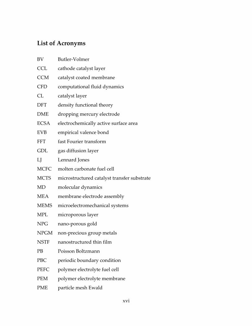
List of Acronyms

BV Butler-Volmer

CCL cathode catalyst layer

CCM catalyst coated membrane

CFD computational fluid dynamics

CL catalyst layer

DFT density functional theory

DME dropping mercury electrode

ECSA electrochemically active surface area

EVB empirical valence bond

FFT fast Fourier transform

GDL gas diffusion layer

LJ Lennard Jones

MCFC molten carbonate fuel cell

MCTS microstructured catalyst transfer substrate

MD molecular dynamics

MEA membrane electrode assembly

MEMS microelectromechanical systems

MPL microporous layer

NPG nano-porous gold

NPGM non-precious group metals

NSTF nanostructured thin film

PB Poisson Boltzmann

PBC periodic boundary condition

PEFC polymer electrolyte fuel cell

PEM polymer electrolyte membrane

PME particle mesh Ewald

xvii

PTFE polytetrafluoroethylene

PZC potential of zero charge

SAX small angle X-ray spectroscopy

SEM scanning electron microscopy

SOFC solid oxide fuel cell

SPC single point charge

SPC/E extended single point charge

STEM scanning transmission electron microscopy

TEM transmission electron microscopy

TIP3P transferable intermolecular potential, three- position

TIP4P transferable intermolecular potential, four- position

UTCL ultrathin catalyst layer

1

1. Introduction

1.1. The global energy infrastructure

Since the mid-19th century, fossil fuels have been the primary energy

source for human society, with applications ranging from fueling the steam

engines, to automobiles and industries, generating electricity, as well as heating

houses. In 2008, 87% of the world’s primary energy was supplied from non-

renewable sources [1]. Energy consumption of a society per capita is directly

related to its welfare standards. An ever-increasing energy consumption rate has

given human society unprecedented welfare and health standards in its history.

However, the global energy infrastructure is undergoing a dramatic

transition: The oil production cannot grow with the same pace as energy demand

due to reduction of reservoirs pressure and ultimate depletion, leading to the oil

peak phenomenon. Fossil fuels are finite resources and the lavish use of energy

from their burning has adverse environmental effects. The main product of the

combustion process, CO2, is a greenhouse gas and contributes significantly to the

global warming phenomenon. The importance of the use of environmentally-

friendly energy sources is most notable in urban areas: The exhaust gas from

cars’ internal combustion engines contains toxic species of CO and NOx, which

represent human health hazards.

2

These concerns drive international initiatives to developing renewable

energy technologies, relying both on primary energy sources (bioenergy, direct

solar, hydropower, wind, and geothermal), as well as secondary sources (fuel

cells, batteries, supercapacitors).

The electrochemical reaction of hydrogen with oxygen produces water

and generates electricity. Utilizing hydrogen as fuel for the propulsion of

vehicles is a highly efficient and potentially sustainable option for the future of

transportation, which could drastically reduce the health and environmental

concerns. A hydrogen fuel cell is the device in which this reaction occurs.

Prototypes of fuel cell powered vehicles were produced by major automobile

companies such as Toyota, Nissan, Mercedes Benz, GMC, Chevrolet, and Honda;

commercial models are planned to be produced by 2017.

So far, fuel cell vehicles have met the required power density, durability,

and stability levels for use in commercial vehicles, and the current challenge for

their commercialization is their cost. Recent cost models of fuel cell vehicles [2],

[3] show strong dependence of the cost on the loading of platinum which is used

as the catalyst. High platinum price and its low utilization in current catalyst

layer (CL) designs motivate extensive research toward increasing the Pt

utilization and lowering the Pt loading in fuel cells.

1.2. Overview of fuel cells technologies

Fuel cells are electrochemical cells that convert the energy of a chemical

reaction to electrical energy with high thermodynamic efficiency. The reaction

happens between a fuel and an oxidant at anode and cathode electrodes,

3

respectively. Depending on the range of operating conditions and the intended

application, different types of fuel cells are distinguished which use different

fuels: solid oxide fuel cells (SOFC) and molten carbonate fuel cells (MCFC)

operate at high temperature. They can be fed with a variety of chemicals as fuel,

such as hydrogen, natural gas or carbon monoxide from gasified coal [4], and can

as well operate on a mix of all those. The operating temperature for SOFC is

generally between 500 °C to 1000 °C, and above 650 °C for MCFCs. Recent

advances in fabrication techniques have enabled lowering the temperature range

of SOFCs to 650-850 °C [5] without compromising cell efficiency. The high

temperature is essential for the performance of electrolyte, which is usually a

ceramic material conducting oxygen ions. The ionic conductivity of the

electrolyte decreases at low temperatures, which leads to an increase in the

Ohmic resistance of the cell. The main applications of SOFC and MCFC are

distributed power and backup power generation, and combined heat and power

generation [6]. Few efforts have explored application of SOFCs in mobile

applications [7].

Polymer electrolyte fuel cells (PEFC) operate at temperatures below 100

°C. PEFC have mainly been developed for vehicular devices, most importantly

fuel cell powered automobiles. PEFCs use hydrogen as the fuel in the anode, and

oxygen from air in the cathode, producing only water as a chemical product and

generating electricity. The reactions occurring in PEFC are hydrogen oxidation

reaction (HOR) at the anode, ( ) ( ) , with an equilibrium

electrode potential of , and the oxygen reduction reaction (ORR) at the

cathode, ( ) ( ) ( ) with . The overall cell

4

reaction is ( ) ( ) ( ) with an equilibrium cell potential of

.

The simplified layout of a PEFC is shown in Figure ‎1.1, and Figure ‎1.2

shows the typical design of a PEFC single cell essential components.

Figure ‎1.1. Basic design of PEM fuel cell; hydrogen oxidation reaction occurs

in the anode and oxygen reduction reaction in the cathode. Protons

transport through the PEM, and electrons through the outer electric

circuit.

5

Figure ‎1.2. Schematic cross section of a single fuel cell, adapted from Ref [2]

(not to scale). Current conduction between the cells is through the

bipolar plates; flow fields feed fuel/air to the cell, and GDL

influences the transport of gases and liquid to/from the cell.

1.3. Advances and challenges in design and operation of

cathode catalyst layer

Platinum is the most widely used monometallic catalyst for fuel cells to

date, mainly due to its proper oxygen adsorption energy [8]. The Pt loading,

defined as the mass of Pt per interfacial area of fuel cell electrode, is the most

6

significant parameter affecting the fuel cell cost, according to recent PEFC cost

models [2], [3], [9]. Therefore, a drastic reduction of Pt loading is a central goal to

meet the stringent cost targets for PEFC commercialization in automotive

applications. The current cost target for automotive fuel cell systems is $30/kWh

for the year 2015. The overall cost of a PEFC stack was reduced from $73/kWh in

2008 [10] to $48/kWh in 2012, achieved with a Pt loading of 0.196 mg/cm2 [3].

The ORR at the cathode has sluggish kinetics and it incurs much higher

irreversible potential losses than the HOR; hence it is currently the main barrier

to cheaper and more efficient PEM fuel cells [11]. Major efforts in materials

science and electrode design strive to reduce the voltage losses. Until the mid-

1980s, PEFC catalyst layer was composed of platinum nanoparticles dispersed on

high surface area carbon support, known as Pt-black. An example of carbon

support is Vulcan carbon with 200 m2/g specific surface area. Pt-black was used

at the typical Pt loading rate of 4 mg/cm2 in the cathode. Pt-black showed great

performance and durability features, though at a very high cost that made it

unfeasible for most consumer applications. A milestone in the cathode catalyst

layer (CCL) design was at 1989, when adding Nafion® to the CCL improved

proton transport in the CCL, and enabled reducing Pt loading to below 0.5

mg/cm2 [12] under laboratory setup with excessive gas supply. Wilson et al. [13]

showed that using thermoplastic ionomers enables melt-processing of electrodes,

which enhances the long term performance. Ralph et al. [14] developed a method

to produce the CL at lower cost and high volume with Pt loading of 0.6 mg/cm2.

It consists of mixing Pt nanoparticles with a size distribution in the range of 20-50

Å, a thermoplastic ionomer and carbon support with given ratio to make an ink,

and use a printing apparatus to coat the ink on a carbon fiber paper. This design

7

enabled removing polytetrafluoroethylene (PTFE) from the membrane electrode

assembly (MEA) design. The design concept is being used to date to produce the

CL. Due to the nature of the mixing process during MEA preparation, the local

distribution of Pt, carbon and ionomer cannot be controlled. The typical

thickness of the CL produced this way is 5-10 µm. Fuel cell systems using this

type of catalyst have shown sufficient energy density for use in automotive

applications. However, further cost reduction is required for fuel cell

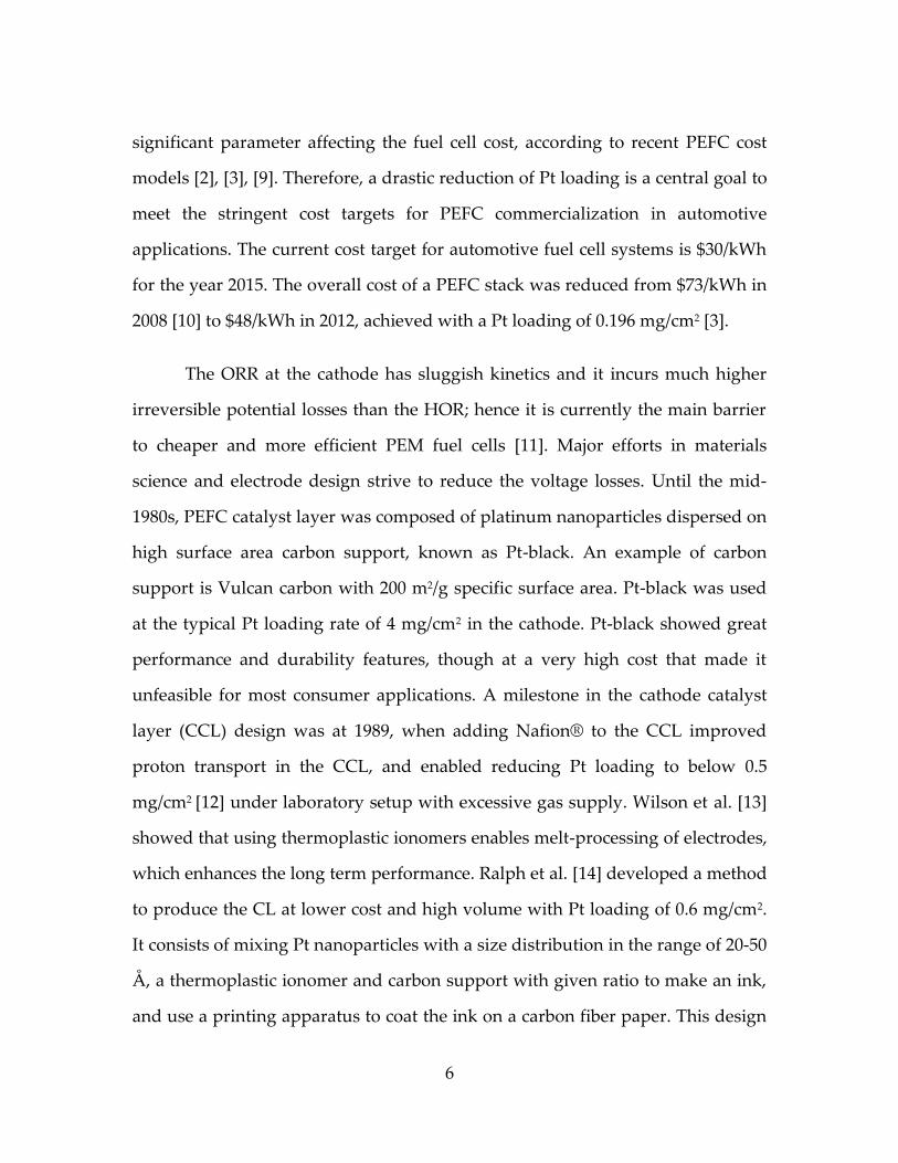
commercialization [15]. Figure ‎1.3 shows the typical Pt/C catalyst material

morphology, and a rival PtCo/C CL exhibiting improved durability features [16].

Figure ‎1.3. TEM image of a)Pt/C catalyst, b)PtCo/C alloy catalyst [16],

random dispersion of Pt particles on the substrate; Reprinted with

permission from Elsevier

Reducing the Pt loading has been pursued through three major strategies:

- Reducing the voltage losses induced by mass transport by modifying the

MEA structure [17],

8

- Enhancing the intrinsic activity of Pt catalyst by using Pt-alloys, which

increases the exchange current density (j0) for the ORR [16], [18–22], or using

non-precious group metals [17], [23] which allows catalyst cost reduction,

- Development of the ultrathin catalyst layer (UTCL) design, relying on

low-resistance mass transport of species through water-filled pores, and

enhancing Pt utilization by increasing the Pt/water interface. We will explain this

strategy in section ‎1.4.

A major shortcoming of the Pt/C catalyst is low utilization of Pt due to the

random distribution of Pt inside CCL. Lee et al. [24] found that the effectiveness

factor of Pt utilization, UPt, in conventional Pt/C CL is around 5%. UPt was defind

as the ratio of the electrochemically active surface area to the total area of Pt in

the CL, estimated from TEM images [25]. The value of 5% UPt, despite the

imprecision, nurtures expectations that a tremendous Pt loading reduction

should be achievable without compromising performance. Another motivation

to develop more stable and durable CLs and catalyst support layers rises from

pronounced electrochemically active surface area (ECSA) loss due to Pt

degradation [26–29].

The CCL is a porous structure, and includes hydrophobic and hydrophilic

pores. Hydrophobic pores allow major fraction of the oxygen transport through

the CL, while hydrophilic pores allow transport of water. The balance between

hydrophobic and hydrophilic pores helps transport of both water and oxygen.

The CCL thickness relates directly with the transport resistance of oxygen

through the CCL. The thickness relates inversely with the effectiveness of Pt in

the catalyst layer [30]. Furthermore, Pt and ionomer distribution in the CL can

9

affect the performance of the cell via tuning current density generation across the

CL. An analytical model was developed to predict and optimize the cell current

density [31] by obtaining uniform reaction rates across the CL.

1.4. Ionomer-free ultrathin catalyst layers

In the conventional CCL, oxygen diffuses mainly through gas-filled pores,

proton concentration is controlled by the ionomer loading, and the water product

diffuses out of CCL through the hydrophilic pores, as well as through

vaporization out of the cell. Therefore, the utilization of Pt depends strongly on

the distribution of these phases in the catalyst layer channel. Since the

distribution of Pt, C and ionomer in the CL is essentially random because of the

fabrication method, relatively low amount of Pt would be effectively utilized

[32]. Furthermore, due to the thickness of catalyst layer, there will be non-

homogeneous distribution of reactants [33] in the catalyst layer, resulting in the

non-homogeneous reaction rate along the catalyst layer.

One of the approaches to overcome the low utilization of Pt is using

ionomer-free ultrathin catalyst layers [34], where oxygen and protons would

diffuse through water to react on the Pt catalyst. Continuity of Pt film catalyst

ensures electrical conductivity of catalyst to the current collector, thus removing

the need for carbon substrate. Thinness of the catalyst layer reduces transport

resistance for oxygen diffusion and proton migration; in fact, the reaction

penetration depth [35] is typically longer than the UTCL thickness.

Different methods for producing the UTCLs include magnetron

sputtering of either several discrete patches or a continuous film of Pt or Pt alloy

10

nanoparticles on a support material [36–38], deposition on nafion membrane[39],

or deposition on gas diffusion layer [40]. UTCLs are 20-30 times thinner than

conventional CL [41], and have drastically lower Pt loading than conventional

CL [42]. Table ‎1.1 summarizes the major characteristic differences of UTCL with

conventional Pt/C CLs. Figure ‎1.4 shows a schematic view of a UTCL design,

fabricated in 3M Company.

Table ‎1.1. Characteristic differences of Pt/C and UTCL

Property Pt/C CL UTCL

Thickness 5-10 μm 0.1-0.5 μm

Main structural characteristic Ionomer-impregnated

Ionomer-free

Proton concentration Fixed by ionomer Determined by electrostatic interaction with charged walls

Pt loading in fuel cell 0.4 mg.cm-2 0.1 mg.cm-2

Figure ‎1.4. SEM images of: a)Pt/C electrode, b) UTCL with 3M NSTF design,

c) Magnified view of NSTF [43], ionomer-free nature of the UTCL

makes the performance depend on the local reaction conditions on

the CL. Reproduced by the permission of the Electrochemical

Society

11

Depositing Pt nanoparticles on nanoporous gold leaf is another method

for UTCL fabrication. Figure ‎1.5 shows images of the substrate and Pt coating.

Unlike the 3M design, there is no necessity for continuity of the Pt film, since the

porous substrate is conductive.

Figure ‎1.5. a) SEM image of NPG. b) High resolution TEM image of NPG. c)

TEM of Pt-coated NPG UTCL at a loading of 0.05 mg.cm-2. d) High

resolution TEM of Pt-coated NPG, image from Ref. [44],

Reproduced by the permission of the Electrochemical Society

Pt deposition on dealloyed nickel through a solvothermal reduction

process is another option for UTCL fabrication. In this method, Ni(II)

acetylaacetonate Ni(acac)2 and Pt(II) acetylaacetonate Pt(acac)2 are boiled

together and then cooled down. Then the organic capping material is removed

and the alloy will then nucleate and form nanoparticles [45]. Figure ‎1.6 shows an

example of such UTCL.

12

Figure ‎1.6. SEM image of Ni75Pt25 nanoparticle for UTCL fabrication, Ni(II)

acetylaacetonate concentration in fabrication process: A) 0.1, B)0.2,

C)0.3, D)0.5 M, Reprinted with permission from [45], Copyright

(2013) American Chemical Society

Experimental studies on UTCLs have shown enhancements in

performance, durability, and stability in these layers [36], [41–43]. However, the

lack of fundamental knowledge in the principles of UTCL operation, as well as

practical issues such as water management [43] and metal cation contaminations

diffused to the catalyst pores from the membrane or GDL, originated from the

fabrication process, leave challenge for research on UTCLs.

The UTCL entails different challenges from Pt/C CL for modeling studies.

Thinness of the catalyst layer (100-500 nm) reduces the resistance of oxygen

transport in the catalyst layer to small values. Water, which can cause flooding in

the conventional catalyst layer, is the carrier of both protons and oxygen to the

reaction sites; therefore, the catalyst layer is utilized best under flooded

condition.

13

An important example of industrially commercialized UTCL is the

nanostructured thin film (NSTF) CLs fabricated by 3M Company. The design

specification that differentiates 3M NSTF from other types of UTCL is the organic

molecular solid substrate, which forms a crystalline whisker, and acts as support

for Pt layer. Since 3M NSTF is the only commercially available type of UTCL to

date, several studies have been carried out on characterizing these layers, and

recent fuel cell models consider this type of CL as a benchmark for fuel cell mass-

production economic calculations [3].

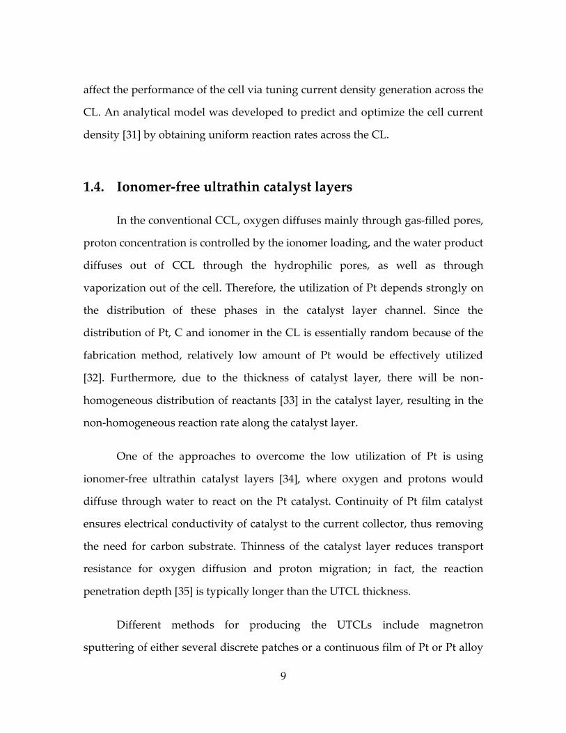
Figure ‎1.7 shows that NSTF electrode has 0.2-0.6 µm thickness, and the

channel size (areas between substrate whiskers) exhibit distribution between 2 to

200 nm. On the substrate whiskers of NSTF, Pt is deposited to form a continuous

layer. Continuity of the Pt layer is important to assure electric connection of all Pt

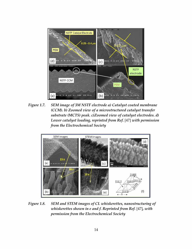
site to the electrode. The deposited Pt film forms a corrugated surface, as shown

in Figure ‎1.8, that consist of so-called whiskerettes. Pt exhibits different surface

facets, depending on the size of the formed whiskerettes [46].

14

Figure ‎1.7. SEM image of 3M NSTF electrode a) Catalyst coated membrane

(CCM). b) Zoomed view of a microstructured catalyst transfer

substrate (MCTS) peak. c)Zoomed view of catalyst electrodes. d)

Lower catalyst loading, reprinted from Ref. [47] with permission

from the Electrochemical Society

Figure ‎1.8. SEM and STEM images of CL whiskerettes, nanostructuring of

whiskerettes shown in e and f. Reprinted from Ref. [47], with

permission from the Electrochemical Society

15

Unlike conventional Pt/C catalyst layers, all NSTF pores are hydrophilic,

and produce significantly more water per unit volume than their conventional

counterparts. Thus, the catalyst layer is flooded more easily due to the thinness

of NSTFs. There are strategies to prevent flooding in catalyst layer, such as

removing the water produced in cathode from anode side GDL [48].

NSTF CCLs have shown significant improvements of fuel cell

performance. The tests under well controlled conditions that suppress the

flooding of porous gas transport layers show that MEA with NSTF technology

on the cathode side exhibits improved performance compared to the MEA with

conventional CCL. The NSTF layers obliterate the need for ionomer

impregnation, while still providing a large ECSA due to the improved water

absorption in the hydrophilic pore network. Furthermore, experimental studies

on UTCLs with NSTF technology have shown significant enhancements in

catalyst durability and stability [36], [41], [49].

There have been efforts to develop analytical models of the

electrochemical phenomena in UTCLs [32], [50–53]. In a recent pore-scale model

by Chan and Eikerling [51], catalyst layer pores were modeled as water-filled

cylindrical channels with smooth walls at given radius, length and metal

potential. A schematic of the investigated model system is shown in Figure ‎1.9.

In this model, the proton and potential distribution along the channel was

calculated using Poisson-Nernst-Planck theory, and the oxygen distribution is

governed by Fickian diffusion of oxygen in water. The channel property

controlling the potential distribution is the surface charge density at the channel

walls. The Stern double layer model was used to relate the surface charge density

16

with the Pt potential of zero charge (PZC). Solution of the model provided the

distributions of reactants, electrolyte phase potential, reaction rates along the

pore, as well as the overall pore effectiveness of Pt utilization. Channel

performance was characterized via the effectiveness factor of Pt. The

effectiveness factor was defined as the actual (predicted) current density

normalized by the reference current density that would be obtained, if reactants

and potential were distributed uniformly in the channel.

Smooth Pt walls

Constant metal potential

PEM boundary

conditions:

Constant proton

concentration

No oxygen flux

GDL boundary

conditions:

Constant oxygen

concentration

No proton flux

Smooth cylindrical Pt channel

O2 diffusion H+ migration

r

L

Reaction plane (OHP)

Reaction plane (OHP)

Figure ‎1.9. Schematic illustration of Chan and Eikerling continuum-type pore-

scale model system [51]

An important aspect in modeling cathode CL is sluggish ORR kinetics,

which enables decoupling electrostatic and kinetic contributions to the

effectiveness factor. This concept was employed in Ref. [51], and it is used in the

current work as well, to assess the effect of electrostatic effectiveness of the

catalyst without explicitly accounting for kinetic effects.

The impedance model of such system revealed the effect of metal surface

charge density on the resistive and capacitive elements of the equivalent circuit

of a water-filled pore [52]. In the limiting cases of fast diffusion of either of the

species, and the case of blocked electrode, exact analytical expressions were

17

derived. Schmuck and Berg [53] scaled up the results of a the single pore model,

to obtain the macroscopic transport equations based on the microscopic pore

level phenomena.

1.5. Local reaction conditions in catalyst layer

The ionomer-free nature of UTCL entails different local reaction

conditions than conventional Pt/C CLs. Distributions of protons and electrolyte

phase potential in UTCL are not determined by the distribution of ionomer but

by electrostatic effects in water-filled pores, as rationalized in [51].

Unlike the random porous structure of conventional Pt/C catalyst layers,

the geometry of UTCL is controlled during the fabrication process. Therefore, the

reactant concentrations can be predicted using established physical theories:

metal surface charge distribution at any given point inside catalyst could be

predicted by an electric double layer model, proton distribution by Poisson-

Nernst-Planck theory, oxygen concentration by Fickian diffusion, and water

transport by Navier-Stokes transport equations [51], [54]. Therefore, local current

generation and reactivity could be predicted, and the local effectiveness could be

determined. This insight introduces an advantage for modeling: we could

perform pore scale or sub-pore scale modeling, and obtain useful insight into

electrocatalytic phenomena in the CL.

18

1.6. Water in nanoconfinement

During the past few decades, tremendous progress has been made in

synthesis of carbon nanotubes, artificial zeolites, porous electrodes and

miniaturization of channels with diameter in the order of a few water molecules.

These developments led to remarkable advances in many fields of application,

including but not limited to electrocatalysis, separation, filtering,

microelectromechanical systems (MEMS), textile engineering and biophysics.

Carbon nanotube has shown diverse applications, ranging from support

material for fuel cell catalyst [21], to nanopipettes [55] and molecular detection

[56]. The ability to transport fluids with precise rate is central to many of the

applications. Zeolite has been applied in separation of either gas [57] or liquid

[58] from gas mixtures. Its separation depends on the pore size distribution in the

zeolite, and affects the adsorption isotherm of the adsorbant. Both carbon

nanotube and zeolites are examples of nanostructured porous media, in which

knowledge of the transport of fluids has led to technological advancements.

The developments in design and application of the nanostructured porous

media have aroused the interest of researchers in the fundamental theories

governing the behavior of fluids under confinement at the nanometer scale. One

of the most important liquids considered is water. Water is the most abundant

and important liquid in nature, however it is by no means a simple fluid: Polarity

and hydrogen bond network of water have caused anomaly in both its bulk and

confined properties.

19

Navier-Stokes equations are the general approach to describe the

transport phenomena of fluids; they form the basis of computational fluid

dynamic (CFD) methods. However, these equations are based on the continuity

of fluids, and break down when the critical dimension of flow becomes

comparable to the size of molecules. The critical size of pores at which continuity

equations break down is a topic of controversy in the scientific community [59],

[60].

Molecular modeling offers an alternative for continuum modeling of

confined water, by explicitly considering the effects of molecular size of water,

bond configurations, charge distributions, and dipole effects. Theories for

describing water potential date back to 1933, when the work of Bernal and

Fowler [61] presented consistent properties of water with those observed in X-

ray spectroscopy. Within the realm of classical molecular simulation, the work of

Rahman and Stillinger [62] was one of the first. Later models improved the

description of water in computer simulations. TIP3P [63] and SPC [64] models

could predict structural properties of water close to experimentally observed

values from neutron diffraction experiment [65]; however, self-diffusion

coefficients are significantly higher than the experimentally observed value [66].

Modifying the SPC model resulted in development of SPC/E model [67],

which improved the prediction of self-diffusion coefficient. SPC/E remains the

most popular 3-site water model to date.

In TIP4P [68] and TIP5P models [69], fictitious particles were added,

which represent the lone electron pair of oxygen. This modification increases the

20

accuracy of dipole moment prediction. However, these models are more

computationally expensive to implement in an MD simulation.

Describing the independent H+ species is not practical in classical MD

simulation; however, the forcefield could be parameterized to account for proton

in the form of hydronium ion (H3O+). In this case, bonded interaction is assumed

between oxygen with three indistinguishable hydrogen atoms. However, it

cannot account for the exchange of protons between two neighboring water

molecules. A more realistic view of proton transport in water was presented in

the empirical valence bond (EVB) model [70], which links ab-initio calculations to

classical MD. The model accounts for exchange of protons by considering a

superposition of two states such as (H3O+…H2O) or (H2O…H3O+) [71]. Using

coupling between different states, it could be used to predict formation of Eigen

and Zundel forms of proton [72]. Expansions of the two-state to multistate EVB

model has been used by the group of Schmickler to describe proton transport on

Pt catalyst [73].

1.7. Scope of the thesis

Chapter 2 of the thesis explains the model of catalyst layer nanochannel

with controlled corrugation, along with its limitations and assumptions. Chapter

3 explains the methodology used in this work: It couples a combination of

continuum-type modeling and classical molecular dynamics to predict the

proton and potential distributions in a catalyst layer nanochannel of Pt with

corrugated walls. Chapter 4 presents and discusses the findings of this work,

how nanostructuring affected proton and water distribution in the catalyst layer

21

channels, and how it is related to the effectiveness factor of CL. We conclude and

highlight the major findings of this work in chapter 5, and make suggestions for

future work.

22

2. Model Description

2.1. UTCL structural parameters

The main microscopic characteristics of a generic UTCL are the ionomer-

free nature, nano-porosity with high surface area, thinness (compared to

conventional CLs), and excess electric charge on the metal surface. Therefore, a

model of UTCL performance must accommodate these aspects.

The nano-porous structure of the catalyst corresponds to high ECSA,

which is a major advantage for fuel cell catalysts. Typical pore sizes in UTCL are

in range of 5-50 nm. Pt deposited on the nanoporous gold leaf has an ECSA of 60

m2/g for a Pt loading of 0.03 mg/cm2 [44]. NiPt nanoparticles have an ECSA of 48

m2/g for 8 nm-diameter NiPt nanoparticle supported on glassy carbon [45], and

3M NSTF shows an ECSA of 10-25 m2/g [47]. The effectiveness of Pt utilization

has reverse dependence on the pore size, as shown for the model of a smooth

cylindrical pore [51]. Figure ‎2.1 shows an inverse relation of Γ with pore radius,

and an inverse relationship of Γ with , due to an increase in the negative

excess charge accumulated on the pore walls upon a decrease in potential. The

inset plot shows the charge-potential relation, derived from the Stern electric

double layer model.

23

Figure ‎2.1. Electrostatic effectiveness vs potential for different pore radii.

Inset: corresponding surface charge density vs potential, image

from Ref. [51], reproduced by the permission of the Electrochemical

Society.

The thickness of UTCLs is in the range of 0.2-0.6 μm, which is 20-30 times

smaller than conventional Pt/C CL. Comparing this thickness with the typical

oxygen penetration depth inside the pore [74] (20 μm for ηc=-0.5 V [52]) shows

small oxygen diffusion resistance in the channel; therefore the concentration of

oxygen can be assumed as uniform along the channel.

The relation between metal surface charge density and metal potential is

not clearly known; however classical double layer models and an estimation of

the potential of zero charge could be used to establish such a relation. This

approach will be discussed in section ‎2.5.

2.2. Model system

In this study, we consider a nanostructured water-filled Pt channel that

represents the interior part of cathode catalyst layer. We consider saw-tooth-

24

shaped modulations on two Pt surfaces, which are mirror images of each other.

The structure is determined by three independent geometrical parameters:

structuring angle θ, channel opening dc and groove width dpp. A schematic

illustration of the channel geometry is shown in Figure ‎2.2. The values of these

parameters that were considered in this work are shown in Table ‎2.1. In each

simulation set, combinations of θ and one other structural parameter was

investigated. The present model can be considered an extension to the model of

Chan and Eikerling [51], with the effect of geometrical surface roughness at the

atomistic level being added.

In addition to the geometric effect, saw-tooth-shaped structuring of the

metal walls gives rise to an inhomogeneous charge distribution on the metal

surface. The surface charge density distributes in a way that makes an

equipotential surface with the potential of φM. Distribution of charge on the CL

surface will be explained in the next chapter.

Figure ‎2.2. Model system schematics, three geometric parameters (θ,dc, dpp)

and metal potential(φM) determine the system

25

The channel walls are made of Pt, and the channel is filled with water and

hydronium ions, H3O+. Periodic boundary conditions (PBC) are applied to the

model system in all directions. The simulated system consists of two identical

grooves. The reason for this choice is to minimize the effect of periodic boundary

conditions on the proton distribution maps.

Table ‎2.1 Range of parameters for investigation of channel structuring

effects

Parameter Value Unit

Structuring angle (θ) 0, 15, 30, 45, 60, 75 Degrees

Channel opening (dc) 10, 20, 30, 40, 50, 60, 80, 100 Å

Roughness Opening (dpp) 20, 30, 40, 50, 60, 70, 80 Å

Metal Potential (φM) -10 -50 -70 -100 -110 mV

2.3. Effectiveness of the catalyst layer channel

In electrocatalysis, the effectiveness factor quantifies the comparison of

different catalysts: It is defined as the ratio of actual reaction rate to an reference

rate that would be obtained if the whole catalyst surface was exposed to equal

concentrations of reactants and equal potentials. Using the cathodic branch of

Butler-Volmer (BV) equation, the local current density, j, generated at the catalyst

surface is calculated by

(

)

(

)

(

( )) ‎2.1

26

where j0 is the exchange current density, the oxygen concentration on the

Helmholtz plane, the proton concentration on the Helmholtz plane, the

oxygen reaction order of ORR, the proton reaction order of ORR, and αc the

cathodic transfer coefficient. The superscript “0” indicates the reference

condition, under which the exchange current density j0 was calculated. We

defined Helmholtz plane to be a plane parallel to the channel walls, at 4 Å

distance from the channel walls.

Local and total effectiveness can be calculated from equations ‎2.3 and ‎2.4,

comparing the actual current generation with the reference case (i), where the

proton and water distributions are equal to the well-defined values at the

boundary,

(

)

(

)

(

( )) ‎2.2

∫

‎2.3

The integration in equation ‎2.3 is done on the surface of Helmholtz plane,

and ds represents a surface element of the Helmholtz plane. Thinness of UTCL

implies small resistance of oxygen transport in the channel, and sluggish kinetics

of ORR allows for assumption of separation of electrostatic and kinetic

contribution to effectiveness, and assuming electrochemical equilibrium inside

the channel, the electrostatic effectiveness depends solely on the proton and

potential distribution, and it is defined as in equation ‎2.4.

27

(

)

(

( )) ‎2.4

Assumption of electrochemical equilibrium allows relating the potential

and concentration of protons inside the channel, thus expressing the

effectiveness relation only in terms of proton concentration,

(

) ‎2.5

where ̃ is the species’ electrochemical potential, and is the chemical potential.

We chose the reference potential at a point in solution, where proton

density is 1.25 M, corresponding to a typical effective proton density in the PEM.

However, PEM proton concentration is the maximum for the CL channel,

occurring on the PEM/CL boundary; typical proton density value in the CL

would be significantly smaller. However, choosing a high value of proton

concentration corresponds to large cathode overpotential values, assuring that at

the given potential, the Pt is not oxidized. Furthermore, having larger number of

protons in the channel offers a better statistical ensemble for protons. The system

consisted of 10-100 protons, 8000-20000 water molecules, and 6000-9000 Pt atoms

in the channel structure.

28

2.4. Limitations for using continuum modeling

In our model, each facet of the structured Pt channel is only a few

nanometers wide. At this scale, surface roughness at molecular scale is

significant, and has notable impact on the surface structure. Therefore, the

approximation of a “smooth” surface fails. Classical MD accounts for all Pt atoms

explicitly, and assigns mass, charge and Lennard-Jones interaction parameters to

each atom.

At the continuum level, Poisson-Boltzmann model describes the relation

between proton concentration and potential. It neglects the finite size of protons,

and proton-proton interactions. The role of solvent is treated in continuum

approximation. A full atomistic MD simulation, on the other hand, accounts for

molecular correlation and interactions, leading to a more accurate description of

the proton interactions at the interface.

The structure of water is not accounted for in continuum modeling.

Physical properties of water at interfaces are different from those in the bulk.

Hydrophobic or hydrophilic nature of the surface and its electric charge affect

the structure of adjacent water. In classical double layer models, the role of

interfacial water has either been neglected, or water is considered as a medium

with known dielectric constant [75]. In the case of nanochannels, important

phenomena occur at the interface, where effects of interfacial charging and the

structure of interfacial water layers must be accounted for.

29

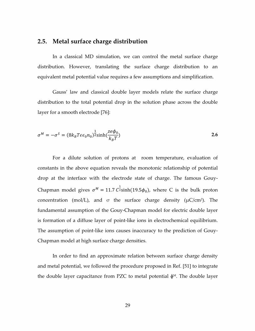
2.5. Metal surface charge distribution

In a classical MD simulation, we can control the metal surface charge

distribution. However, translating the surface charge distribution to an

equivalent metal potential value requires a few assumptions and simplification.

Gauss’ law and classical double layer models relate the surface charge

distribution to the total potential drop in the solution phase across the double

layer for a smooth electrode [76]:

( ) (

) ‎2.6

For a dilute solution of protons at room temperature, evaluation of

constants in the above equation reveals the monotonic relationship of potential

drop at the interface with the electrode state of charge. The famous Gouy-

Chapman model gives

( ), where C is the bulk proton

concentration (mol/L), and σ the surface charge density (μC/cm2). The

fundamental assumption of the Gouy-Chapman model for electric double layer

is formation of a diffuse layer of point-like ions in electrochemical equilibrium.

The assumption of point-like ions causes inaccuracy to the prediction of Gouy-

Chapman model at high surface charge densities.

In order to find an approximate relation between surface charge density

and metal potential, we followed the procedure proposed in Ref. [51] to integrate

the double layer capacitance from PZC to metal potential ɸM. The double layer

30

capacitance in the Stern model [76] is given by

, where CH is the

Helmholtz layer capacitance, and Cdiff the diffuse layer capacitance, given by

( )

( ) ‎2.7

where HP indicates the position of Helmholtz plane. A typical value for CH is

~0.2 F.m-1, and a typical value for Cdiff is ~3 F.m-1 [76].

Since CH is usually significantly smaller than Cdiff, the capacitance can be

assumed dominated by CH; furthermore we assume CH to be constant. Therefore

we can integrate CH to obtain surface charge density:

∫ ( ) ( )

‎2.8

For ( ) constant it gives ( ), and thus

( ) .

Therefore, in order to calculate ɸM, we need to estimate CH and have prior

knowledge of ɸPZC. Measuring ɸPZC is straightforward for liquid electrodes such

as dropping mercury electrode (DME), where varying the potential affects the

surface tension of mercury, and enables measuring the differential capacitance of

mercury. Consequently, the minimal capacitance is measured at ɸPZC. However,

studying solid electrodes is experimentally difficult. There exist experimental

difficulties for studying solid electrodes such as Pt, including reproducibility of

electrode surfaces, solution contamination, specific adsorption of anions, oxidie

31

formation on the surface, as well as maintaining a clean surface during the

experiment. Moreover, the value of ɸPZC is not unique for a polycrystalline

surface. Mimicking the double layer phenomena has been attempted by

ultrahigh vacuum systems [77] as well as DFT calculations on well-defined

surfaces [78], [79]. The values of ɸPZC for Pt(111) range from 0.1 to 1.0 V in the

literature. However, for an estimate of metal potential, we assume ɸPZC=1.0 V,

and CH=0.24 F.m-1, a typical value measured from differential capacitance

measurement experiments. Table ‎2.2 shows typical corresponding values of

metal potential, potential drop across the double layer and metal surface charge

density.

Table ‎2.2. Typical values of surface charge density and metal potential,

system with θ=45°, dc=60 Å, dpp=30 Å, direct relation between metal

potential and surface charge density

ɸHP-ɸ0(mV)

(M)

σ(μC.cm-2) ɸM(V)

-1 0.20 -5.0 0.78

-10 0.25 -6.1 0.69

-50 0.57 -13.9 0.35

-70 0.84 -20.4 0.05

32

3. Simulation Methodology

3.1. Overview

In this chapter, we explain how model systems are generated, MD

simulations are run, and the trajectory results are analyzed. The general

procedure is explained, and the detailed discussions follow in the subsequent

sections.

As mentioned in the previous chapter, each model system is identified

with four parameters (θ, dc, dpp, φM). With these parameters we construct specific

Pt channel geometries (section ‎3.2) and calculate partial charges on Pt surface

atoms (section ‎3.3). Then we calculate the total charges on the Pt surface, and add

an equal number of protons to the channel interior to counterbalance the

negative charge on the walls. The concentration of water in the channel is

maintained at a value close to 55 mol/L.

In the next step, we performed energy minimization on the system.

Thereafter, the system was thermally annealed between 800 K and 300 K.

Production runs were performed for 4 ns on the system (section ‎3.4).

Production runs were analyzed to explore equilibrium properties of the

system (section ‎3.5). Our data analysis focused on three major aspects: (i) density

maps of hydronium ion distributions were analyzed to determine potential

distribution and the channel electrostatic effectiveness factor (section ‎3.5.1), (ii)

33

temporal water displacement data was analyzed to calculate water self-diffusion

coefficient in the channel (section ‎3.5.2), (iii) water distribution maps were

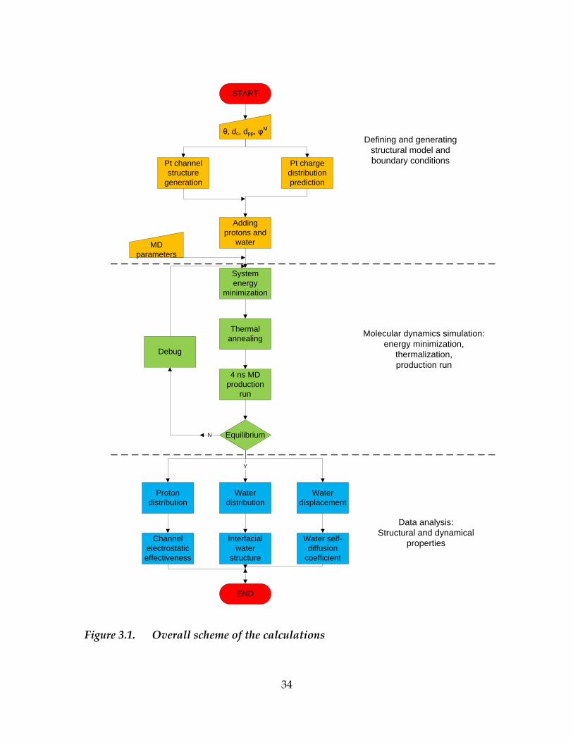
analyzed to identify interfacial water layers (section ‎3.5.3). Figure ‎3.1 shows the

overall scheme of calculations. In the following sections, we will explain the

detailed approaches.

34

Pt channel

structure

generation

θ, dc, dpp, φM

Pt charge

distribution

prediction

Adding

protons and

water

System

energy

minimization

Thermal

annealing

4 ns MD

production

run

EquilibriumN

MD

parameters

Water

distribution

Y

Proton

distribution

Water

displacement

Water self-

diffusion

coefficient

Interfacial

water

structure

Channel

electrostatic

effectiveness

END

START

Defining and generating

structural model and

boundary conditions

Molecular dynamics simulation:

energy minimization,

thermalization,

production run

Data analysis:

Structural and dynamical

properties

Debug

Figure ‎3.1. Overall scheme of the calculations

35

3.2. Pt structure construction

Platinum is a metal with face centred cubic (FCC) crystalline structure,

with lattice constant of a=3.92 Å. The unit cell of the Pt crystal lattice is shown in

Figure ‎3.2.

Figure ‎3.2. Primitive cell of Pt crystal with FCC structure

In order to construct a Pt nanochannel, we first created a cube of Pt by

replicating the unit cell in x,y,z directions. Then, the structural parameters were

used to calculate the plane equations of the channel walls, and the Pt atoms

located between two walls were removed. Figure ‎3.3 shows an incomplete Pt

channel, for the purpose of better illustration. The depth of the channel was fixed

for all cases, w=5.88 nm, corresponding to 15 times the Pt lattice constant. A 7 Å-

thick Pt layer was considered to both sides of the channel as a clearance layer, in

order to minimize the image charge effects on H3O+ distribution.

36

Figure ‎3.3. Full atomistic Pt channel structure, incompletely constructed to

better illustrate build-up procedure (left), schematic representation

(right). Water and hydronium ions would be added to the space in

the middle of the structured channel.

Figure ‎3.4. 2-d Schematic picture of the model system with physical boundary

conditions

The plane equations indicating channel walls are as follows:

37

( )

( )

‎3.1

( )

( )

‎3.2

( )

( )

‎3.3

( )

( )

‎3.4

( )

( )

‎3.5

( )

( )

‎3.6

( )

( )

‎3.7

( )

( )

‎3.8

The value θ determines the surface Miller indices. The Miller indices will

be multiples of (1, tan(θ), 0). Therefore, in each case we simulate a stepped Pt

surfaces.

For each case, step fraction is defined as 1/n, where n is the number of

atoms on the terrace of each step.

38

( ) ‎3.9

( ) ‎3.10

The two cases of θ=0° and θ=45° generate known smooth surfaces of

Pt(100) and Pt(110), respectively. Cases with 0< θ<45° have terraces parallel to the

xz plane, and cases with 45°< θ<90° have terraces parallel to the yz plane. This

change in the plane direction is the same reason for having two definitions for

step fraction.

3.3. Prediction of charge distribution on Pt nanochannel

surface

According to Gauss’s law, the surface of a conductor is equipotential, and

all free charge on the metal is accumulated on the surface. For a smooth surface,

the metal surface charge density is homogeneous. However, for a “rough”

surface, the charge distribution is inhomogeneous. In this section, we explain

how we assigned partial electric charge to each Pt surface atom in the

nanochannel.

Potential distribution inside the channel was predicted using the

numerical solution of Poisson-Boltzmann (PB) equation,

( )

(

( )

) ‎3.11

39

where ( ) is the number density of protons, dielectric constant of water,

the reference proton concentration, kB Boltzmann constant, and T the absolute

temperature, set to 300 K.

We assumed dielectric constant of , where is the vacuum

permittivity, and

, as the reference concentration. Boundary

condition for this problem is constant metal potential on the walls ( ) for

boundaries 1-4 and 7-10 in Figure ‎3.4, and symmetry (

) on boundaries

number 5 and 6.

The PB equation has an analytical solution only for simple geometries. For

geometries like the present case, the PDE could only be solved numerically. We

used triangular meshing and finite element method in COMSOL Multiphysics ®

package to obtain the numerical solution to this partial differential equation.

We calculated the surface charge density by evaluating the potential

gradient at the metal boundary and using

. The “surface Pt atoms” are

located within a distance of 3Å away from ideal wall positions. The total surface

area is

( ), and the interfacial area per surface atom is

,

where nsurf is the number of surface Pt atoms.

Therefore, the partial charge of each atom, q’, is calculated as:

( ) ‎3.12

40

where

is the elementary charge. The total charge on the

surface is calculated by adding up all charges on surface atoms ∑

.

The ensemble is made electroneutral by adding a corresponding correct

number of hydronium ions to the system. Thus, the total charge on the surface

must be a correct number. Since Q’ is not essentially an integer, we cut it to the

closest integer value, and normalized all q’ values: [ ] ⇒

, where

is the partial charge assigned to each surface Pt atom. Q is the total charge on

the surface, and |Q| equals the number of hydronium ions that must be added to

the system to counterbalance the wall charges.

3.4. Classical molecular dynamics

We have used classical MD to find equilibrium distribution of protons and

water in the nanochannel. In this chapter, we first introduce the basic concept of

MD, and explain the procedures and parameters we used to simulate the system.

The theory is discussed in detail in Ref. [80]. The calculations were carried out

using the GROMACS [81] open source package.

3.4.1. Description of the forcefields used

Classical MD calculation is based on integrating Newton’s equation of

motion for each species in the system,

. The force exerted on each atom is

calculated as in equation ‎3.13. (Bold-faced variables indicate vectors.)

‎3.13

41

where FB is the bonded (intramolecular) interactions of an atom, described

by harmonic oscillator approximation as stated in equations ‎3.14 and ‎3.15.

( )

( )

‎3.14

( ) ( )

| | ‎3.15

FB was calculated only on hydronium ions and water molecules, since Pt channel

atoms were assumed frozen at their positions.

Forces due to non-bonded interactions, FNB, include Van der Waals

interactions, described by Lennard Jones interactions (FLJ), and charge-charge

interactions described by Coulomb’s law (FCoulomb),

( )

( )

, (

( )

( )

)

| |, ‎3.16

| | ‎3.17

Having calculated the force, new position and velocity of each atom can

be calculated by discretizing the equation of motion using leapfrog finite

differencing scheme [82] for velocity calculation, (

) (

)

( ) , and position calculation, ( ) ( ) (

) . The time step

chosen was 2 fs, commonly used in the literature. It was tested, though, that the

42

simulation systems would crash with time steps larger than 2.4 fs, due to

interaction of species beyond the cut-off range, leading to blowing up of the

molecules within the system.

The overall scheme of force calculation parameters is shown in Figure ‎3.5.

Figure ‎3.5. Force calculation scheme

In our model, Pt atoms were fixed to their position throughout the

simulation. Calculation of partial charges of Pt atoms was explained in the

previous section. The interaction of Pt with other atoms was calculated by fitting

an n-body Sutton-Chen potential [83] to Lennard Jones form, the same procedure

as followed in Ref. [84]. Forcefield parameters of H3O+ were taken from Ref. [85].

We chose the SPC/E water model [67] for this study. If used with the

GROMOS43 forcefield, this water model gives the self-diffusion coefficient of

( )

[86], which is close to the experimental

43

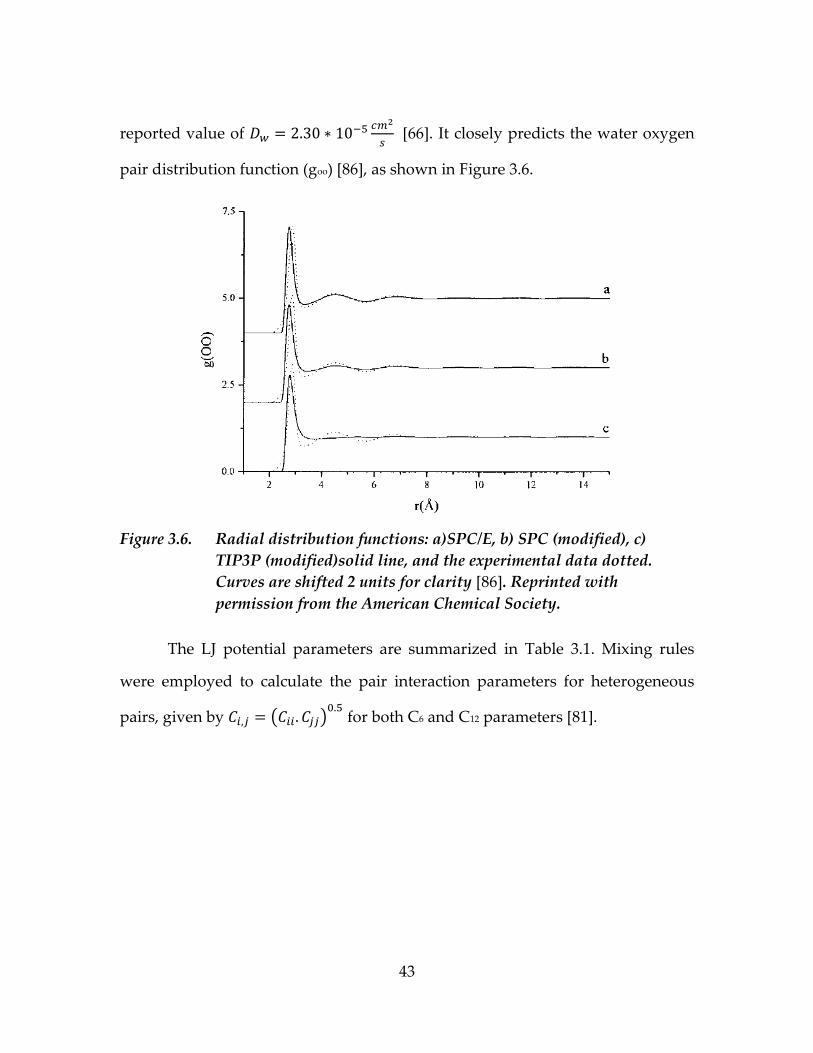
reported value of

[66]. It closely predicts the water oxygen

pair distribution function (goo) [86], as shown in Figure ‎3.6.

Figure ‎3.6. Radial distribution functions: a)SPC/E, b) SPC (modified), c)

TIP3P (modified)solid line, and the experimental data dotted.

Curves are shifted 2 units for clarity [86]. Reprinted with

permission from the American Chemical Society.

The LJ potential parameters are summarized in Table ‎3.1. Mixing rules

were employed to calculate the pair interaction parameters for heterogeneous

pairs, given by ( )

for both C6 and C12 parameters [81].

44

Table ‎3.1. Van der Waals interaction parameters for the system species

Pair C6(kJ.nm6) C12(kJ.nm12) q (e)

Pt-Pt 0.015 2.98*10-6 See text

O-O (water) 0.003 2.63*10-6 -0.848

O-O (hydronium ion) 0.003 2.63*10-6 -0.248

H-H (water) 0.00 0.00 0.424

H-H (hydronium ion) 0.00 0.00 0.416

3.4.2. Computational details

We simulated an infinite nanochannel, using periodic boundary condition.

Therefore, we had to make sure that the finite cell size did not introduce

significant artifacts on the proton distribution diagrams of the system, which

could stem from insufficient number of exchange of species through the periodic

boundaries. The effect of finite simulation cell size is noticeable especially when

the system consists of ions with long range electrostatic interactions, such as the

system of this study. The artifacts caused due to long range electrostatic

treatment are due to artificial stabilization of the system, which inhibit

conformational fluctuations. Such artifacts have been reported in references [46],

[87], [88]. The Particle Mesh Ewald (PME) is a method [89] employed for systems

with long range electrostatic interactions. In order to capture effects of dipole

(O(1/r3)) and Coulomb (O(1/r)) potentials efficiently, the PME method calculates

the short range forces directly, and calculates the long range forces in Fourier

space[88]. With this method, the computational time scales with the size of the

system,N, as N.log(N); compared to the scaling as N2 in the Ewald summation

method [88].

45

Van der Waals forces have short effective range. Therefore, the forces on

each atom could be estimated with the sum of forces exerted from atoms closer

than a specific “neighboring radius” (chosen 0.9 nm in this work). This choice

drastically increases the force calculation speed. After each 10 MD steps (20 fs)

the list of neighboring atoms must be updated. However, the neighbor searching

algorithm mandates using a small time step of 2 fs. The small time step is

essential for inhibiting dissociation of molecules.

We used the canonical ensemble for this model. Therefore, the system was

coupled to a Berendsen thermostat [90] with a time constant of 1 ps, to keep the

ensemble temperature at 300 K.

All the calculations were done on the scientific computation clusters of

NRC-Institute for Energy, Mining and Environment of Canada in Vancouver,

BC. We used MATLAB v2006a and COMSOL 3.5a for pre-processing and

analysing the simulation results. Gromacs v4.0.3 [81] was used to run MD

calculations. The simulation was run on one node with eight processors. The

typical simulation run time was ~2 ns/day. VMD [91] and RASMOL [92] software

were used for visualization of the results.

3.5. Simulation data analysis

The last 2 ns of the MD trajectory (from a total of 4 ns) represent

equilibrated configurations. After the initial 2 ns of the trajectory, the potential

and kinetic energy of the system do not deviate from the average value by more

than 2%. Proton and water distribution maps are generated by averaging over

46

statistically independent configurations, and water self-diffusion coefficients

were calculated from analyzing water molecule displacements over time.

The analyses lead to the calculation of the electrostatic effectiveness factor

of the channel, water structure and water self-diffusion coefficient.

3.5.1. Hydronium ion density map and electrostatic effectiveness

In order for the electrochemical reaction to occur, hydronium ions need to

approach the surface. We considered the hydronium ions within a distance of 4

Å from the ideal location of walls as “surface protons”. This definition enabled

attributing a single value of proton concentration to each point on the Helmholtz

plane, and mapping the 2-dimensional proton distribution map onto a 1-

dimensional distribution profile. Therefore, calculation of channel effectiveness

reduces to a 1-d integration problem. This task was achieved using MATLAB

image processing toolbox.

The density profile was used to back-calculate the potential profile

adjacent to the surface, assuming a Boltzmann distribution of proton

concentration,

(

). Electrostatic effectiveness factor was

calculated as explained in equation ‎2.4.

3.5.2. Surface and bulk water diffusion

The self-diffusion coefficient of water can be calculated from

| ( ) ( ) |

. We analyzed Dw by distinguishing surface water

and bulk-like water. The water molecules within a distance of 4 Å from channel

ideal wall position in the final trajectory frame were considered surface water,

47

and the rest were considered bulk-like water. Dw for these two groups was

calculated over a period of 200 ps. The trajectory length is chosen short enough,

so that the exchange between the two phases of water is not significant.

3.5.3. Interfacial water structure

In order to investigate the effect of nanoconfinement on water structure,

we calculated the pair correlation function g(r) defined as

( )

∑ ∑

( )

. In statistical mechanics, gi,j(r) shows the

probability of finding species i at radial distance r from species j. g(r) is an

indication of the structure and density of a certain phase. We calculated goo(r) for

both surface water and bulk-like water, and compared the distributions.

48

4. Results and Discussion

4.1. Overview

In this chapter, the results of surface charge, proton and water distribution

in the nanochannel are presented and discussed. Section ‎4.2 presents the results

of surface inhomogeneity on the electric charge distribution on the metal surface.

Section ‎4.3 presents a qualitative analysis of the proton distribution in the

nanochannel. In order to quantify the impact of varying degrees of surface

structuring on electrocatalytic properties of the nanochannel, we calculated the

channel electrostatic effectiveness factor. The results are presented in section ‎4.4.

In section ‎4.5, we present the impact of channel nanostructure on water diffusion

and structure, and section ‎4.6 explains the sensitivity of obtained results to the

parameters employed for simulation.

4.2. Surface charge distribution in the nanostructured channel

On a smooth surface, all the metal atoms have equal surface charge

density. In a structured channel, we noticed that peak positions have the highest

surface charge, and deep positions have the lowest surface charge. Typical

potential, surface charge distribution and proton concentration maps are shown

in Figure ‎4.1.

49

Figure ‎4.1. Typical distribution maps in the nanochannel predicted by PB

theory: a) potential distribution, b) proton concentration, c)

Electric field contour lines, d) metal surface charge density

Within the investigated range of 1 nm< dc< 10 nm, we observed that dc did

not affect the prediction of surface charge density distribution. Therefore, the

-0.08

-0.07

-0.06

-0.05

-0.04

-0.03

-0.02

-0.01

0

0.E+0

5.E+7

1.E+8

2.E+8

2.E+8

3.E+8

3.E+8

0 20 40 60 80

x (Å)

E q

( 𝑚)

𝑜

𝑚

a b

c d

𝜙( 𝑉

) 𝐸

(𝑉 𝑚)

𝑐 𝐻 𝑂

( 𝑀

)

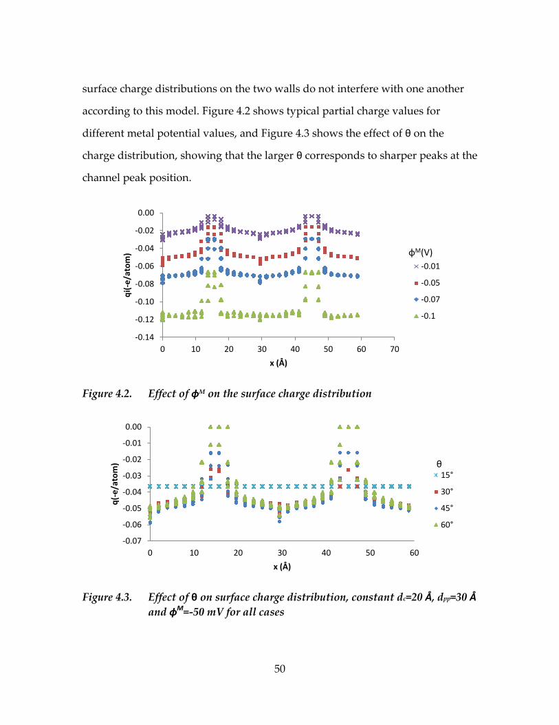
50

surface charge distributions on the two walls do not interfere with one another

according to this model. Figure ‎4.2 shows typical partial charge values for

different metal potential values, and Figure ‎4.3 shows the effect of θ on the

charge distribution, showing that the larger θ corresponds to sharper peaks at the

channel peak position.

Figure ‎4.2. Effect of ɸM on the surface charge distribution

Figure ‎4.3. Effect of θ on surface charge distribution, constant dc=20 Å, dpp=30 Å

and ɸM=-50 mV for all cases

-0.14

-0.12

-0.10

-0.08

-0.06

-0.04

-0.02

0.00

0 10 20 30 40 50 60 70

qi(

-e/a

tom

)

x (Å)

-0.01

-0.05

-0.07

-0.1

ɸM(V)

-0.07

-0.06

-0.05

-0.04

-0.03

-0.02

-0.01

0.00

0 10 20 30 40 50 60

q(-

e/a

tom

)

x (Å)

15°

30°

45°

60°

θ

51

Figure ‎4.3 shows that the surface charge density distribution for θ=15° is

almost homogeneous. This observation is expected from such channel geometry,

since the structure is similar to a Pt (100) smooth surface with weak roughening,

as shown in Figure ‎4.4. The observation of almost homogeneous σ distribution

holds for all θ<15° values.

Figure ‎4.4. Pt structured channel with θ=15°, predicted charge distribution

close to homogeneity

4.3. Hydronium ion distribution in catalyst layer channels

4.3.1. Hydronium ion density distribution in smooth Pt channels

Equilibrium distribution of hydronium ions on a smooth catalyst surface

is uniform along the surface. Variation of ion density perpendicular to the

surface is determined according to the electrochemical equilibrium in the

channel. Continuum-type models have been able to predict distribution

prediction for simple geometries of the channel. Engstroem and Wennerstroem

have analytically solved the Poisson-Boltzmann (PB) equation for geometry of

two parallel slabs [93], with the boundary condition of constant surface charge

density on two parallel charged slabs. Andelman has solved the PB equation for

52

other cases with simple geometry [94]. In the absence of counter-ions in the

solution, potential and hydronium ion distribution were calculated as below.

Figure ‎4.5. Schematic of analytically solved electrostatic model system

( )

( ( )), with

, ‎4.1

( )

( )

,

‎4.2

where nm denotes the hydronium ion density at the center of the channel (z=0),

and 1/K is the characteristic length scale of the system.

In order to confirm the consistency of molecular dynamics calculations

with this theory, we performed 10 cases of MD simulations of hydronium ions

and water distribution on slab-like channels with smooth walls of Pt(111) at

various openings and surface charge densities. We investigated the hydronium

ion density distribution perpendicular to the Pt walls. The results indicated

overall agreement between the two approaches in the channel interior, although

the effect of finite size of atoms is not captured in the PB model prediction. A

53

simple schematic of this difference is shown in Figure ‎4.6. Due to these

differences between the two models, the maximum proton concentration was

observed 1 Å further from the surface in an MD calculation. We also observed a

typical layering behavior, which is not predicted in the PB theory. The

discrepancy between the two models was reflected more clearly in systems with

high surface charge density and with smaller groove width. The two predictions

could be deemed matching for systems with channel spacing over 7 nm and

surface charge density smaller than

. Sample results from the calculations

are shown in Figure ‎4.7.

Figure ‎4.6. Wall position definition for PB theory, the wall position is not

defined precisely in an MD simulation; however the positions of all

atoms nuclei are known.

54

a

b

c

Figure ‎4.7. Hydronium ion number density at σ=-16.8 μC.cm-2 and channel

openings of a)2 nm, b) 3 nm, c) 4 nm, better agreement between PB

and MD results at larger channel opening

4.3.2. Hydronium ion distribution in nanostructured channels

We investigated hydronium ion density distributions on CL channels, to

observe how metal nanostructuring causes deviation from uniform distribution

0

1

2

3

4

5

-4 -2 0 2 4

c x(1

/ n

m3)

x(nm)

MD

PB

0

1

2

3

4

-4 -2 0 2 4

c x(1

/ n

m3)

x (nm)

MD

PB

0

0.5

1

1.5

2

2.5

-4 -2 0 2 4

c x(1

/ n

m3)

x(nm)

MD

PB

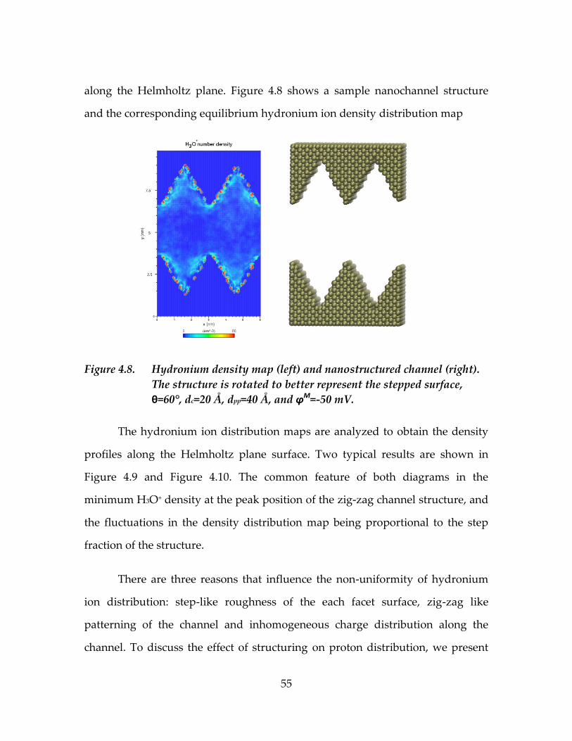
55

along the Helmholtz plane. Figure ‎4.8 shows a sample nanochannel structure

and the corresponding equilibrium hydronium ion density distribution map

Figure ‎4.8. Hydronium density map (left) and nanostructured channel (right).

The structure is rotated to better represent the stepped surface,

θ=60°, dc=20 Å, dpp=40 Å, and φM=-50 mV.

The hydronium ion distribution maps are analyzed to obtain the density

profiles along the Helmholtz plane surface. Two typical results are shown in

Figure ‎4.9 and Figure ‎4.10. The common feature of both diagrams in the

minimum H3O+ density at the peak position of the zig-zag channel structure, and

the fluctuations in the density distribution map being proportional to the step

fraction of the structure.

There are three reasons that influence the non-uniformity of hydronium

ion distribution: step-like roughness of the each facet surface, zig-zag like

patterning of the channel and inhomogeneous charge distribution along the

channel. To discuss the effect of structuring on proton distribution, we present

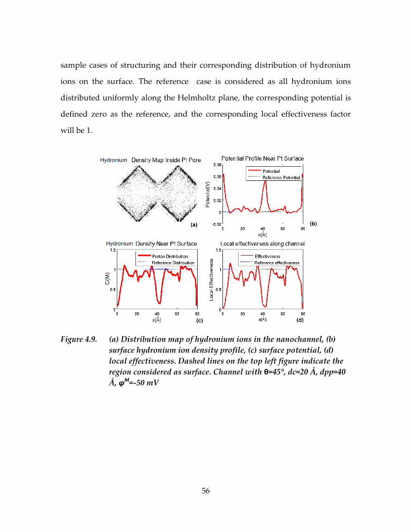
56

sample cases of structuring and their corresponding distribution of hydronium

ions on the surface. The reference case is considered as all hydronium ions

distributed uniformly along the Helmholtz plane, the corresponding potential is

defined zero as the reference, and the corresponding local effectiveness factor

will be 1.

Figure ‎4.9. (a) Distribution map of hydronium ions in the nanochannel, (b)

surface hydronium ion density profile, (c) surface potential, (d)

local effectiveness. Dashed lines on the top left figure indicate the

region considered as surface. Channel with θ=45°, dc=20 Å, dpp=40

Å, φM=-50 mV

57

Figure ‎4.10. (a) Distribution map of hydronium ions in the nanochannel, (b)

surface hydronium ion density profile, (c) surface potential, (d)

local effectiveness. Dashed lines on the top left figure indicate the

region considered as surface. Channel with θ=75°, dc=20 Å, dpp=30 Å,

and φM=-50 mV

Although the two chambers in the simulation cell are identical, the proton

density profile along the surface does not show complete symmetry in all cases.

The observation suggests that either the equilibrium condition has not been

obtained, or the sampling has been insufficient. We changed the Van der Waals

and electrostatic force calculation cut-off values; however, no significant change

was observed neither in proton distribution maps nor water mean square

displacement plots. Some results are shown in sections ‎4.6.2, ‎4.6.3, and ‎4.6.6.

Appearance of a local minimum hydronium ion density at the peaks of

the zig-zag pattern was unexpected, since these points carry the highest negative

58

surface charge density. A possible reason for this behavior is the walls maximum

repulsion at the peaks.

The electrostatic repulsion between two nanochannel walls reaches

maximum at the peak position. The peak positions have the shortest distance

from each other, and carry the highest amount of similar charge. We suggested

that these effects lead to depletion of H3O+ in the peak region. In order to test this

hypothesis, we compared H3O+ density at the peak position for different channel

openings. Increasing channel opening decreases overlapping, and is expected to

increase H3O+ density at the peak. For this comparison, we set θ=45° and dpp=30

Å and

constant, and varied dc between 10 Å and 100 Å. We observed

that H3O+ density at the peak increased with increase of the channel opening, but

the minimum at the peak position remains. Reducing double layer overlap by

increasing dc does not remove the unexpected minimum at the peak. The results

are shown in Figure ‎4.11.

Figure ‎4.11. Relative H3O+ density at channel peak region vs. dc, effect of walls

electrostatic repulsion on H3O+ depletion from peak region, with

constant θ=45°, dpp=30 Å, and φM=-50 mV

0.15

0.2

0.25

0.3

0.35

0.4

0 20 40 60 80 100 120

C/C

0

dc(Å)

59

4.4. Electrostatic effectiveness factor as a function of channel

structure

We showed how the channel structure affects proton distribution in the

catalyst layer channel. However, so far we did not comment on whether this

structuring led to enhancement or deterioration of channel performance. To

address this question, electrostatic effectiveness factor was introduced in chapter

2. Since the activity is normalized to the total Helmholtz plane area, the

electrostatic effectiveness factor shows the effect of structuring on channel

performance beyond changing the active surface area.

4.4.1. Effect of channel opening and structuring angle

In order to investigate the effect of channel opening on electrostatic

effectiveness, we varied the structural parameters as per table below.

Table ‎4.1. Range of parameters for investigation of channel opening effect

Parameter Value Unit

Structuring angle (θ) 0, 15, 30, 45, 60, 75 Degrees

Channel opening (dc) 10, 20, 30, 40, 50, 60, 80, 100 Å

Groove width (dpp) 30 Å

Metal potential (φM) and

average surface charge density (σ)

-10 (-5), -50 (-14) mV (

)

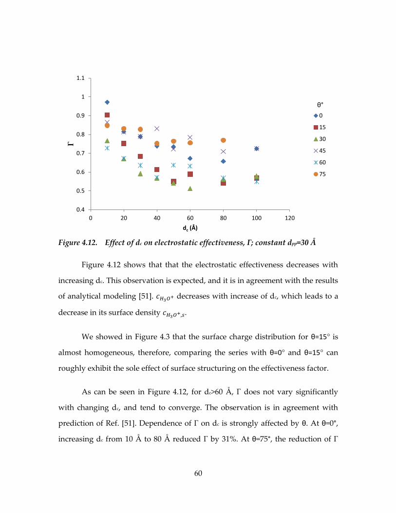
60

Figure ‎4.12. Effect of dc on electrostatic effectiveness, Γ; constant dpp=30 Å

Figure ‎4.12 shows that that the electrostatic effectiveness decreases with

increasing dc. This observation is expected, and it is in agreement with the results

of analytical modeling [51]. decreases with increase of dc, which leads to a

decrease in its surface density .

We showed in Figure ‎4.3 that the surface charge distribution for θ=15° is

almost homogeneous, therefore, comparing the series with θ=0° and θ=15° can

roughly exhibit the sole effect of surface structuring on the effectiveness factor.

As can be seen in Figure ‎4.12, for dc>60 Å, Γ does not vary significantly

with changing dc, and tend to converge. The observation is in agreement with

prediction of Ref. [51]. Dependence of Γ on dc is strongly affected by θ. At θ=0°,

increasing dc from 10 Å to 80 Å reduced Γ by 31%. At θ=75°, the reduction of Γ

0.4

0.5

0.6

0.7

0.8

0.9

1

1.1

0 20 40 60 80 100 120

Γ

dc (Å)

0

15

30

45

60

75

θ°

61

was only 8%. This sensitivity is attributed to the change of channel volume at

different θ, as given by

( ( )) ⇒

( ) ‎4.3

Therefore, at large θ, the volume change is weakly affected by dc. Consequently Γ

is weakly related to dc. Γ is a monotonic function of surface proton ratio, as

expected from equation ‎2.4. We investigated the correlation between Γ and the

overall in the channel. Figure ‎4.13 shows this relationship.

Figure ‎4.13. Direct effect of overall H3O+ concentration on channel effectiveness,

dispersion of data in the low concentration region is the channel

structure-specific effects.

0.4

0.5

0.6

0.7

0.8

0.9

1

0 0.5 1 1.5 2 2.5 3 3.5 4 4.5

Γ

0

15

30

45

60

75

( )

θ°

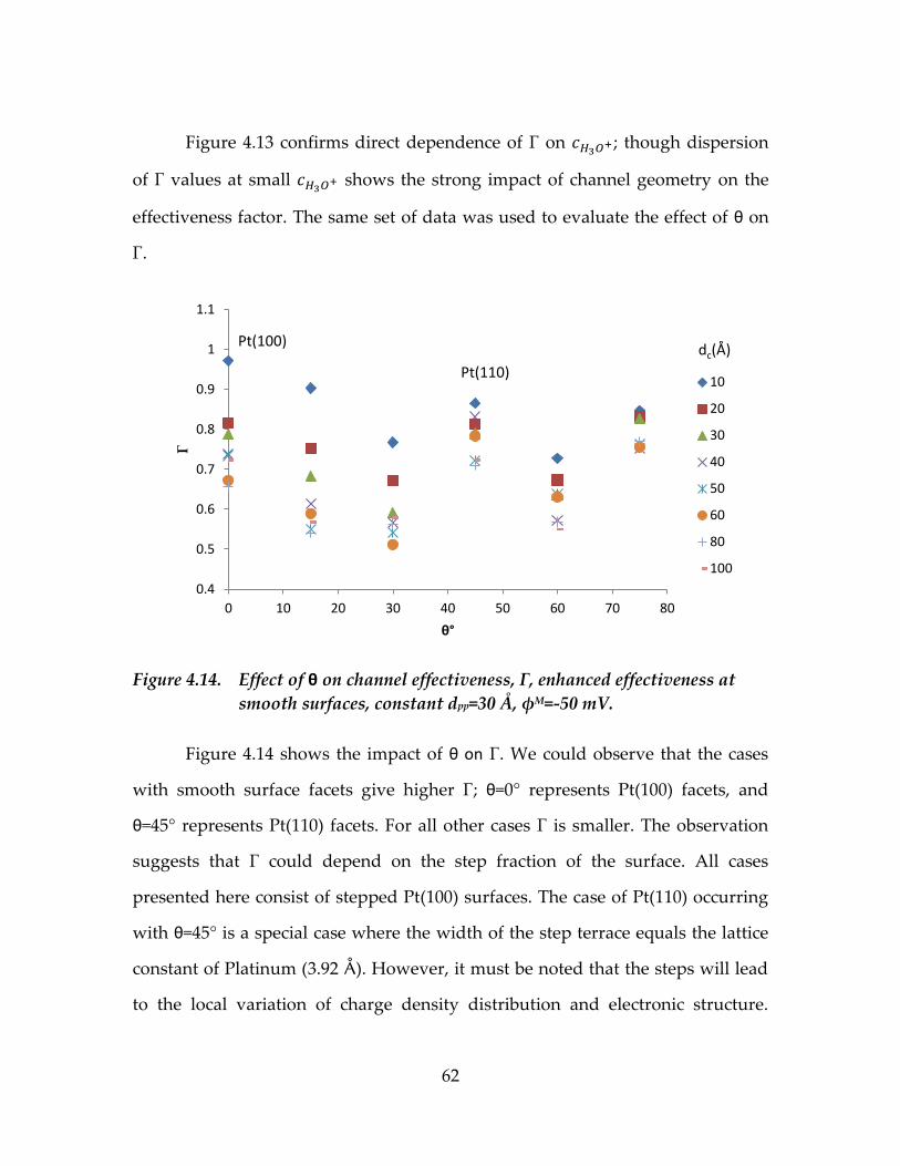
62

Figure ‎4.13 confirms direct dependence of Γ on ; though dispersion

of Γ values at small shows the strong impact of channel geometry on the

effectiveness factor. The same set of data was used to evaluate the effect of θ on

Γ.

Figure ‎4.14. Effect of θ on channel effectiveness, Γ, enhanced effectiveness at

smooth surfaces, constant dpp=30 Å, φM=-50 mV.

Figure ‎4.14 shows the impact of θ on Γ. We could observe that the cases

with smooth surface facets give higher Γ; θ=0° represents Pt(100) facets, and

θ=45° represents Pt(110) facets. For all other cases Γ is smaller. The observation

suggests that Γ could depend on the step fraction of the surface. All cases

presented here consist of stepped Pt(100) surfaces. The case of Pt(110) occurring

with θ=45° is a special case where the width of the step terrace equals the lattice

constant of Platinum (3.92 Å). However, it must be noted that the steps will lead

to the local variation of charge density distribution and electronic structure.

0.4

0.5

0.6

0.7

0.8

0.9

1

1.1

0 10 20 30 40 50 60 70 80

Γ

θ°

10

20

30

40

50

60

80

100

dc(Å) Pt(100)

Pt(110)

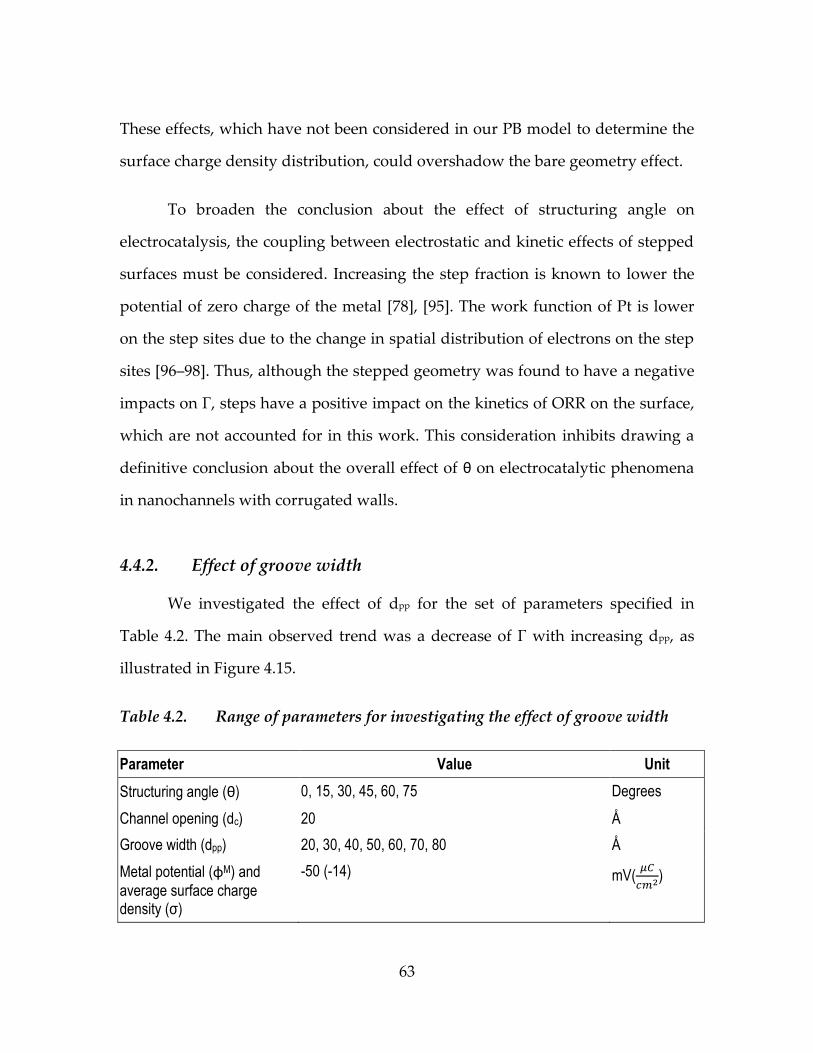
63

These effects, which have not been considered in our PB model to determine the

surface charge density distribution, could overshadow the bare geometry effect.

To broaden the conclusion about the effect of structuring angle on

electrocatalysis, the coupling between electrostatic and kinetic effects of stepped

surfaces must be considered. Increasing the step fraction is known to lower the

potential of zero charge of the metal [78], [95]. The work function of Pt is lower

on the step sites due to the change in spatial distribution of electrons on the step

sites [96–98]. Thus, although the stepped geometry was found to have a negative

impacts on Γ, steps have a positive impact on the kinetics of ORR on the surface,

which are not accounted for in this work. This consideration inhibits drawing a

definitive conclusion about the overall effect of θ on electrocatalytic phenomena

in nanochannels with corrugated walls.

4.4.2. Effect of groove width

We investigated the effect of dpp for the set of parameters specified in

Table ‎4.2. The main observed trend was a decrease of Γ with increasing dpp, as

illustrated in Figure ‎4.15.

Table ‎4.2. Range of parameters for investigating the effect of groove width

Parameter Value Unit

Structuring angle (θ) 0, 15, 30, 45, 60, 75 Degrees

Channel opening (dc) 20 Å

Groove width (dpp) 20, 30, 40, 50, 60, 70, 80 Å

Metal potential (ɸM) and

average surface charge density (σ)

-50 (-14) mV(

)

64

Figure ‎4.15. Inverse effect of groove width on electrostatic effectiveness of

nanochannel, constant dc=20 Å

Increasing dpp while keeping dc and σ fixed reduces in the

nanochannel. Lower causes decrease of the ratio of hydronium ions on the

surface. The relation between Γ and is shown in Figure ‎4.16.

0.4

0.5

0.6

0.7

0.8

0.9

1

0 20 40 60 80 100

Γ

dpp (Å)

0

15

30

45

60

75

θ

65

Figure ‎4.16. Direct effect of overall H3O+ density on Γ, constant dc=20 Å

We used the data from this set of simulations to evaluate the effect of θ.

The results attest to our former hypothesis of the effect of step fraction on

channel effectiveness. Step fraction does not vary with changing dc, nor with dpp.

Therefore, similar behavior is expected in the case of varying dpp. However, some

discrepancy is observed, which arises from the variation of inside the

channel. Increasing dpp reduces the overall inside the channel, consequently

reducing . Reduction of overall hydronium ion concentration on the

surface implies smaller Γ in the nanochannel.

0.4

0.5

0.6

0.7

0.8

0.9

1

0 0.5 1 1.5 2

Γ

0

15

30

45

60

75

θ

( )

66

Figure ‎4.17. Effect of θ on Γ, constant dc, inverse relation with surface step

fraction

4.4.3. Effect of metal surface charge density

A higher value of |σM| increases the Coulomb attraction between protons

and the negatively charged channel walls, and it increases in the channel.

The values chosen for this study are reported in Table ‎4.3. The results are

presented in Figure ‎4.18.

Table ‎4.3. Range of parameters for investigating the effect of surface charge

Parameter Value Unit

Structuring angle (θ) 0, 15, 30, 45, 60, 75 Degrees

Channel opening (dc) 20 Å

Groove width (dpp) 30 Å

Metal potential (ɸM) and

average surface charge density (σM)

-5, -10, -50, -70, -100, -110 (-5 .. -50) mV(

)

0.4

0.5

0.6

0.7

0.8

0.9

1

0 10 20 30 40 50 60 70 80

Γ

θ°

20

30

40

50

60

70

80

dpp(Å)

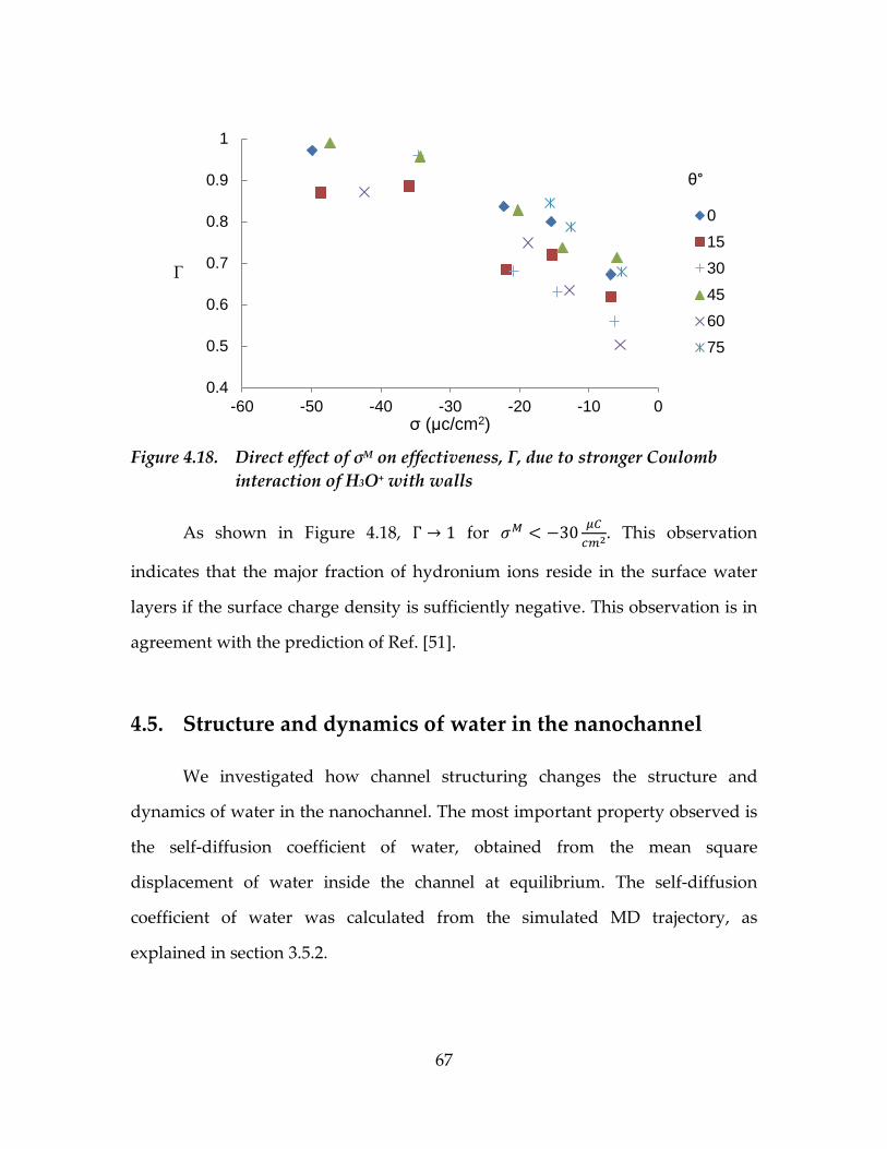
67

Figure ‎4.18. Direct effect of σM on effectiveness, Γ, due to stronger Coulomb

interaction of H3O+ with walls

As shown in Figure ‎4.18, for

. This observation

indicates that the major fraction of hydronium ions reside in the surface water

layers if the surface charge density is sufficiently negative. This observation is in

agreement with the prediction of Ref. [51].

4.5. Structure and dynamics of water in the nanochannel

We investigated how channel structuring changes the structure and

dynamics of water in the nanochannel. The most important property observed is

the self-diffusion coefficient of water, obtained from the mean square

displacement of water inside the channel at equilibrium. The self-diffusion

coefficient of water was calculated from the simulated MD trajectory, as

explained in section ‎3.5.2.

0.4

0.5

0.6

0.7

0.8

0.9

1

-60 -50 -40 -30 -20 -10 0

Γ

σ (μc/cm2)

0

15

30

45

60

75

θ°

68

For all cases, we evaluated whether a plot of log(MSD) vs log(t) is linear.

We employed this relation as a test whether equilibrium of water had been

obtained. We also investigated the structuring of water at the surface by

analyzing the auto-correlation function of water molecules, as explained in

section ‎3.5.3. In a refined analysis, we evaluated the structure and dynamics of

surface and bulk-like water. Several experimental and theoretical works have

confirmed the existence of the two distinct phases of water. In this work, we

considered water molecules in a slab of 4 Å distance from the metal wall position

as surface water, and the rest as bulk-like water. We assumed the subsets did not

exchange water molecules for 200 ps. The error bars on the self-diffusion

coefficient diagrams indicate the statistical RMS deviation of MSD vs. t from a

straight line.

The value of 4 Å is estimated to be the maximum distance up to which a

charge transfer reaction could occur. Increasing this value to higher numbers

diminishes the existing distinctions between different nanochannels to a great

extent.

4.5.1. Two phase water structure in the channel

Density maps of water, like the one shown in Figure ‎4.19, reveal that a

highly structured layer of water exists at the metal interface. Figure ‎4.19 shows

formation of two phases of water in the nanochannel, due to the confinement

effect. We refer to the phase adjacent to the channel wall “surface water” and the

phase with homogeneous density distribution “bulk-like water”.

69

Figure ‎4.19. Typical water density map, high contrast of colors indicate a

highly structured phase

4.5.2. Effect of the channel opening and structuring angle on water self-

diffusion coefficient

The self-diffusion coefficient of water, Dw, increases with dc. The value

approaches a plateau at the limit of dc>10 nm. Within the range of our

investigation, the maximum Dw value is 10% below the Dw predicted by the bulk

SPC/E water model [86].

The structuring angle θ has a weak yet discernible effect on Dw. The

variation of Dw with θ is due to the direct dependence of channel volume on θ.

Therefore, the effect of θ on Dw is more pronounced at small dc values.

Figure ‎4.20 shows that at dc=10 Å, the difference in Dw between θ=0° and θ=75°

70

cases is

, but the difference drops to

when dc=80 Å. The

competing effect of dc and θ is on volume change, due to the following relation,

( ( )) ( ) [ ( )

] ‎4.4

It shows that the effect of dc on volume is more pronounced at small θ values.

The result can be expressed in terms of the ratio of the number of bulk-like water

molecules to the number of surface water molecules.

Figure ‎4.20. Effect of dc on water self-diffusion coefficient, Dw

0

0.5

1

1.5

2

2.5

3

0 20 40 60 80 100 120dc(Å)

0°

15°

30°

45°

60°

75°

θ Dw,bulk= 2.

𝐷𝑤 ( 𝑐𝑚

𝑠)

71

Figure ‎4.21. Analyzing the effect of channel opening on Dw in terms of ratio of

bulk-like (nb) to surface (ns) water ratio

Figure ‎4.21 shows that the effect of dc and θ on Dw can be attributed to

tuning the ratio of number of bulk-like to number of surface water molecules. It

could equally be analyzed as the volume to area ratio of the channel, too. Self-

diffusion coefficient of each phase of water (bulk-like/surface) shows weak

dependence to dc. Figure ‎4.20 shows the existence of two distinct phases of water

with their specific Dw. However, the dependence of Dw,b to the bulk to surface

water ratio indicates the high exchange rate during the analysis time (200 ps)

between bulk-like and surface water at small bulk to surface ratios.

0

0.5

1

1.5

2

2.5

3

0 2 4 6 8 10 12

0°

15°

30°

45°

60°

75°

θ

(

𝑚

)

72

Figure ‎4.22. Dependence of Dw to channel structure, a) surface water, b) bulk-

like water

4.5.3. Effect of groove width on water self-diffusion coefficient

The effect of dpp is similar to dc. Increasing dpp increases the channel

volume to wall area ratio, as shown below,

( ( ) ( )) ⇒

( )

( ) ‎4.5

Consequently, the

ratio increases, which leads to the increase of Dw with dpp.

The results are shown in Figure ‎4.23.

0

0.5

1

1.5

2

2.5

3

0 5 10

(

𝑚

)

0

0.5

1

1.5

2

2.5

3

0 5 10

15°

30°

45°

60°

75°

θ

(

𝑚

)

a b

73

Figure ‎4.23. Effect of groove width on water self-diffusion coefficient, Dw, dc=20

Å constant.

4.5.4. Effect of metal charging on water self-diffusion coefficient

The interaction of water with the metal surface is a charge-dipole

interaction. Variation of σM influences the water dynamics in the channel. Over

the investigated range of parameters, we could observe a slight decrease of Dw

with |σM|. The reason is stronger immobilization and preferential ordering of

water at the interface due to increasing strength of interaction with the

negatively charged walls. The results are shown in Figure ‎4.24.

0

0.5

1

1.5

2

2.5

3

0 10 20 30 40 50 60 70 80 90

dpp(Å)

0

15

30

45

60

θ°

𝐷𝑤(

𝑐𝑚

𝑠)

𝑚

74

Figure ‎4.24. Effect of Pt surface charge density on water self-diffusion

coefficient, constant dc=20 Å dpp=30 Å

This effect can be evaluated separately for surface and bulk-like water. As

we would expect, the effect of σM on Dw is more pronounced on surface water

through charge-dipole interactions. The results are shown in Figure ‎4.25.

0

0.2

0.4

0.6

0.8

1

1.2

1.4

1.6

-60 -50 -40 -30 -20 -10 0

σ(μC/cm2)

0°

15°

30°

45°

60°

𝑊(

𝑚

) θ

75

Figure ‎4.25. Dependence of Dw on Pt surface charge, a) bulk-like water, b)

surface water

4.6. Sensitivity analysis to MD run parameters

It is essential to make sure that the obtained results are not highly affected

by the choice of computational parameters. In chapter 2 we mentioned how the

range of structural parameters was chosen for this study. In chapter 3,

parameters used in the MD run were introduced, and the reasons for choosing

them were explained. In this section, we show how the results for different

channel geometries would vary with changing computational parameters, MD

run time, forcefield and long-range electrostatic treatment method, as well as the

nature of catalyst metal.

0

0.2

0.4

0.6

0.8

1

1.2

1.4

1.6

1.8

2

-60 -40 -20 0

σ(µC/cm2)

(

𝑚

)

0

0.2

0.4

0.6

0.8

1

1.2

1.4

1.6

1.8

2

-60 -40 -20 0

σ(µC/cm2)

15°

30°

45°

60°

75°

(

𝑚

)

θ θ

a b

76

4.6.1. Total simulation run time

All simulations were run for a total of 4 ns. The final 2 ns were sampled as

equilibrium configurations. The configuration ensemble was sampled each 10 ps,

resulting in 200 frames for analysis. For a nanochannel with θ=45°, dc=20 Å,

dpp=30 Å and average surface charge density of

we extended the

simulation to 10 ns, and extracted the coordinates every 10 ps. The results

showed negligible fluctuation of Γ values. This assured us that the chosen 4 ns

run time has been sufficient.

Figure ‎4.26. Sensitivity of calculated effectiveness factor to analyzed trajectory

length

4.6.2. Choice of forcefield and intermolecular interactions

Hydronium ion distribution in the nanochannel is determined by the

charge-charge interaction with surface Pt atoms. It does not change significantly

with variations to Lennard-Jones parameters of water and Pt. Though, a few

models were proposed for partial charges of a hydronium ion. In the current

0102030405060708090

[0-1] [0-2] [2-4] [4-6] [6-8] [8-10] [6-10]

Effectiveness% 84.6 83 81.3 80.7 80.5 81.6 80.6

84.6 83 81.3 80.7 80.5 81.6 80.6

Γ%

Trajectory analysis time (ns)

[0-1]

[0-2]

[2-4]

[4-6]

[6-8]

[8-10]

[6-10]

77

work we used the values reported by Goddard et. al. [85] consistently, and no

further investigations was done in this regard.

Water is described by SPC/E model, and the model is calibrated to be used

with the GROMOS43a forcefield. Test simulations were run with SPC and TIP3P

water models, too, and the results were compared to those of the SPC/E model.

We obtained similar Γ values. The predicted Dw was 10% smaller with TIP3P

model and 7% smaller for TIP3P model. This observation was expected, because

it follows the same trend as predictions of the bulk self-diffusion coefficient of

water, Dw.

4.6.3. Long range electrostatic interaction treatment

We used Particle Mesh Ewald (PME) method. This method is an

approximation to Ewald method, improving the scaling of calculation time with

system size, N, from N2 to N.log(N). The method is essential to implement,

because electrostatic forces are of long range nature, and the interaction of

species with those in neighboring cells must be accounted for.

The minimum recommended short range cut-off for calculation to be used

in the PME method is 0.9 nm [81]. For a sample case we increased the short range

cut-off up to 1.9 nm. The variation of Γ was small, and Dw was not affected at all.

Therefore, we did the calculation with the recommended 0.9 nm. It must be

noted that increasing the PME short range cut-off is accompanied with drastic

decrease in the simulation speed. This dependence was the motivation for

choosing the minimum acceptable PME short range cut-off.

78

Figure ‎4.27 Sensitivity of simulation result and calculation speed to PME

short range force calculation

4.6.4. Temperature

In this study we considered the constant temperature of 300 K. We

performed sensitivity analysis on temperature, and the effect on Γ was found to

be negligible. This observation is in line with the dominance of electrostatic over

thermal effects in the system. The results are shown in Figure ‎4.28.

Furthermore, we investigated the effect of changing the employed

thermostat algorithm from Berendsen to Nose-Hoover. For the same test system,

no significant deviation from the original Γ value was observed.

0

2

4

6

8

10

12

0

0.2

0.4

0.6

0.8

1

0 0.5 1 1.5 2

Sim

ula

tio

n s

pe

ed

(n

s/d

ay)

Γ

PME short range (nm)

79

Figure ‎4.28. Temperature dependence of channel effectiveness for a channel with

θ=45°, dc=20 Å, dpp=30 Å, σ=-14 μC/cm2

4.6.5. Nanochannel material

In the classical MD method, the metal is identified by four parameters:

crystalline structure, lattice constant and the two Lennard-Jones fitting

parameters. We simulated sample channels made of copper and gold, which

have FCC structure. The Lennard-Jones interaction parameters are taken from

Ref. [99], and are reported in Table ‎4.4. The form of Lennard-Jones potential used

is introduced in equation ‎3.14.

Table ‎4.4. Physical properties of Pt, Cu, and Au for MD set-up

Pair Lattice const. (Å) C6 (kJ.nm6.mol-1) C12 (kJ.nm12.mol-1)

Pt-Pt 3.92 1.51*10-2 2.98*10-6

Cu-Cu 3.61 2.23*10-2 3.11*10-6

Au-Au 4.08 5.07*10-2 1.46*10-5

0

0.1

0.2

0.3

0.4

0.5

0.6

0.7

0.8

0.9

280 290 300 325 350 365

Effectiveness 0.82 0.8 0.82 0.83 0.81 0.82

0.82 0.8 0.82 0.83 0.81 0.82

Γ

Temperature (K)

80

Sample calculations were done on channels with θ=45°, dpp=30 Å and ɸM=-

50 mV, and varying dc={20,50, 100} Å. The results are presented in Figure ‎4.29.

Figure ‎4.29 Sensitivity of Γ results to nanochannel material

The results presented in Figure ‎4.29 could be presented in terms of the

metal lattice constant, suggesting direct relation between the effectiveness factor

and the packing of metal atoms, as illustrated in Figure ‎4.30.

Figure ‎4.30. Inverse relation of channel effectiveness with the metal lattice

constant

0.5

0.6

0.7

0.8

0.9

1

0 20 40 60 80 100 120

Γ

dc(Å)

Pt

Au

Cu

0.5

0.6

0.7

0.8

0.9

1

3.5 3.6 3.7 3.8 3.9 4 4.1 4.2

Γ

Lattice constant (Å)

20

50

100

dc(Å)

Au Pt

Cu

81

Figure ‎4.29 and Figure ‎4.30 suggest that there is a slight dependence of Γ

on the nanochannel material. The observation indicates dominance of Coulomb

interaction over the Lennard-Jones interactions.

4.6.6. Pt-Pt Lennard-Jones interaction parameters

In this work, the Lennard-Jones interaction parameters for Pt-Pt pair were

adapted from a similar system [84]. However, to test the sensitivity of results to

the choice of Pt-Pt parameters, we hypothetically changed the parameters by an

order of magnitude and calculated the effectiveness factor. For this purpose,

sample calculations were done for a channel with θ=45°, dc=20 Å, dpp=30 Å and

ɸM=-50 mV with the Lennard-Jones parameters listed in Table ‎4.5.

Table ‎4.5. Pt-Pt Lennard-Jones parameters for sensitivity analysis

Pair C6 (kJ.nm6.mol-1) C12 (kJ.nm12.mol-1) Effectiveness

Pt-Pt (original) 1.51*10-2 2.98*10-6 0.813

Test 1 1.51*10-3 2.98*10-6 0.698

Test 2 1.51*10-1 2.98*10-6 0.890

Test 3 1.51*10-2 2.98*10-7 0.976

Test 4 1.51*10-2 2.98*10-5 0.624

The result confirms the direct relationship of Γ with the attractive branch

(c6) and inverse relationship with the repulsive branch (c12) of the Lennard-Jones

potential. Figure ‎4.31 shows that the effect of the repulsive branch is more

pronounced (~30% change) than the attractive branch (~20% change).

82

Figure ‎4.31. Sensitivity of nanochannel effectiveness to Pt-Pt interaction

parameters

The sensitivity of Dw to the Pt-Pt interaction parameters was also

investigated. We observed an inverse relation of Dw with the attractive coefficient

c6, implying that more hydrophilic confinement reduces water mobility. The

effect of the c12 repulsive parameter was not significant, due to its short range

nature.

Figure ‎4.32. Sensitivity of water self-diffusion coefficient to Pt-Pt interaction

parameters

0.698

0.813 0.89 0.976

0.813

0.624

0

0.2

0.4

0.6

0.8

1

1.E-7 1.E-6 1.E-5 1.E-4 1.E-3 1.E-2 1.E-1 1.E+0

Γ

c-value

c6

c12

1.51

1.224

0.797

1.045 1.224 1.148

00.20.40.60.8

11.21.41.61.8

1.0E-7 1.0E-5 1.0E-3 1.0E-1

c-value

c6

c12

(

𝑚

)

83

4.7. Insight to the effect of nanostructuring on ORR kinetics

The present research investigated the effect of metal nanostructure on the

local reaction conditions in a CL nanochannel. The implicit assumption for this

research is that the catalyst nanostructure did not affect the intrinsic

electrocatalytic activity of the catalyst. This assumption enabled comparison of

nanochannels based on the electrostatic effectiveness factor. The intrinsic reaction

rate is represented as the exchange current density j0 in the Butler-Volmer

equation. However, there is evidence showing that the metal basal plane

structure affects the intrinsic reaction rate. Therefore, it is essential to review the

impact of surface structure on the kinetics of ORR, to predict the effect of

nanostructuring on the overall catalyst effectiveness.

Smoluchowsky [100] showed that the local work function of metals is not

homogeneous on a rough metal surface. The local smoothing of electron density

gives rise to lowering of the work function at the step sites of the metal surface,

which enhances the electrocatalytic activity. The work function was later

correlated with the potential of zero (total) charge of the metal [101]: it was

shown that increasing the step density of a metal has an inverse effect on the

metal PZC for different surfaces as well as nanoparticles [87], [95], [102–105]. The

UTCL pore model of Chan and Eikerling [51] predicted a direct relation between

the value of Pt PZC and catalyst effectiveness factor at a given potential.

84

5. Conclusions

5.1. Results Summary

In this work, we simulated ionomer-free catalyst layer channels with zig-

zag patterning of platinum walls. We investigated the effects of channel

nanostructuring on the equilibrium hydronium ion and water distribution, and

the electrostatic effectiveness factor of Pt utilization in the nanochannel. The

major findings are as follows.

Different structuring angles change the step fraction on the

nanostructured channel. We observed that protons concentrate away from the

steps on each facet. Therefore, the electrostatic effectiveness factor is inversely

related to the step fraction on each facet. In terms of structuring angle, we

observed that smooth facets simulated with θ=0°, representing Pt(100) surface,

and θ=45°, representing Pt(110) surface, exhibited higher values of the

effectiveness factor.

The electrostatic effectiveness is inversely related to the channel opening.

The observation is linked to the reduction of the overall hydronium ion density

in the channel. At constant surface charge density, increasing the channel

opening causes dilution of hydronium ions in water, and consequently lowers

their concentration at the Helmholtz plane.

85

Increasing the groove width does not change the step fraction of facets,

but reduces overall proton concentration in the channel. Therefore, we obtained

an inverse relationship between groove width and effectiveness factor.

Compared to the channel opening effect, the effect of groove width is less

pronounced.

The effectiveness factor of the channel is directly related with the metal

surface charge density. Changing the surface charge density to more negative

values strengthens the attraction between hydronium ions and negatively

charged walls, hence increasing the effectiveness factor. We presented our results

based on surface charge density rather than metal potential, because finding the

exact relation between metal surface charge density and potential requires a

consistent model of metal-solution interface, including the effect of surface oxide

formation; at this time, the understanding of this relation is still sketchy.

However, the investigated potential should be smaller than the platinum

potential of zero charge.

We investigated the effect of nanochannel structuring on the structure and

self-diffusion coefficient of water inside the channel. The correlation was

described best by distinguishing the volume of water on the surface and in the

bulk-like phase. The nanochannel walls hinder the water dynamics strongly at

their surface, and have weaker effect on the bulk-like water phase. Surface water

has self-diffusion coefficient almost three times smaller than bulk-like water.

Water motion is hindered at the interface due to charge-dipole type interaction of

the charged channel walls with water. The bulk-like water phase exhibits a self-

86

diffusion coefficient smaller than that of bulk water, due to the confinement

effect.

The self-diffusion coefficient of water affects oxygen diffusivity in the

channel; however, the effect on the overall electrocatalysis in the cathode is

estimated to be less important than the electrostatic effect: oxygen diffusion

resistance is not the controlling step of ORR in ultrathin ionomer-free catalyst

layers [51].

5.2. Suggestions for future work

It is known that a variation in the step fraction on the catalyst surface

shifts the potential of zero charge [104]. Therefore, stepped surfaces would have

different charging behaviour than smooth surfaces at equal metal potential

values. This effect could be integrated to the prediction of metal surface charge

distribution (described in section ‎3.3). Considering this effect would lead to a

better understanding of the effect of structuring on the CCL performance.

In the current approach, metal surface charge distribution is fixed. It does

not change during the course of a simulation. However, in reality the

arrangement of hydronium ions leads to a redistribution of electric charges at the

interface. Since accounting for mobile surface charges is not already

implemented in the MD code, addressing this problem would be an

improvement of the classical MD code. This would mean considering fictitious

particles to represent electric charges on the metal surface, and allow those

particles to move on the metal surface.

87

We investigated a monoatomic catalyst, and the sensitivity analysis on the

metal material showed that the effect of material manifests itself by its lattice

constant. However, our model does not yet predict the interfacial hydronium ion

distribution for a metallic catalyst deposited on a conductive substrate. Such

systems are the prevailing fuel cell catalysts [38]. For such systems, we must

know the spatial distribution of the potential of zero charge at catalyst, to be able

to predict the surface charge distribution. The design space of the problem can be

then changed to a smooth substrate with different controlled configurations of

catalyst nanoparticles deposited on the surface. This model could be considered

as a piece of the multiscale modeling roadmap of fuel cell catalyst modeling, for

which DFT simulations at the nanoparticle level are conducted in separate works

in our group [22].

The other improvement to the model can come from a more accurate

description of proton and water at the interface. Especially, the two or multi-state

EVB model [70], [106] can be used to provide a more accurate insight on the

proton and water structure at the interface. It must be noted, however, that EVB

is a computationally expensive method, therefore the choice of simulated

systems must be carefully refined.

On the experimental side, the results of this work indicated that smaller

channel opening results in enhanced effectiveness factor of Pt utilization. In a

benchmark design such as 3M NSTF catalysts, this means recommending small

feature sizes of support whiskers.

88

References

[1] W. Moomaw, F. Yamba, M. Kamimoto, L. Maurice, J. Nyboer, K. Urama,

and T. Weir, “Introduction,” in IPCC Special Report on Renewable Energy

Sources and Climate Change Mitigation, O. Edenhofer, R. Pichs-Madruga, Y.

Sokona, K. Seyboth, P. Matschoss, S. Kadner, T. Zwickel, P. Eikemeier, G.

Hansen, S. Schloemer, and C. von Stechow, Eds. Cambridge, New York: ,

2011.

[2] B. D. James, J. A. Kalinoski, and K. N. Baum, Mass Production Cost

Estimation for Direct H 2 PEM Fuel Cell Systems for Automotive Applications :

2009 Update, US department of energy report. 2010.

[3] B. D. James, K. Baum, A. B. Spisak, and W. G. Colella, “Mass-Production

Cost Estimation for Automotive Fuel Cell Systems, US department of

energy report,” 2013.

[4] S. P. S. Badwal and K. Foger, “Solid Oxide Electrolyte Fuel Cell Review,”

Ceramics International, vol. 22, pp. 257–265, 1996.

[5] N. Shaigan, W. Qu, D. G. Ivey, and W. Chen, “A review of recent progress

in coatings, surface modifications and alloy developments for solid oxide

fuel cell ferritic stainless steel interconnects,” Journal of Power Sources, vol.

195, no. 6, pp. 1529–1542, Mar. 2010.

[6] E. Antolini, “The stability of LiAlO2 powders and electrolyte matrices in

molten carbonate fuel cell environment,” Ceramics International, pp. 1–16,

Nov. 2012.

[7] E. Wachsman and K. T. Lee, “Lowering the Temperature of Solid Oxide

Fuel Cells,” Science, vol. 18, pp. 935–939, 2011.

[8] J. K. Nørskov, J. Rossmeisl, A. Logadottir, L. Lindqvist, J. R. Kitchin, and H.

Jonsson, “Origin of the Overpotential for Oxygen Reduction at a Fuel-Cell

Cathode,” Journal of Physical Chemistry C, vol. 108, pp. 17886–17892, 2004.

89

[9] A. Veziroglu and R. Macario, “Fuel cell vehicles: State of the art with

economic and environmental concerns,” International Journal of Hydrogen

Energy, vol. 36, no. 1, pp. 25–43, Jan. 2011.

[10] “Hydrogen and Fuel Cell Activities, Progress, and Plans; Report to the

Congress, US department of energy,” 2009.

[11] L. Carrette, K. a. Friedrich, and U. Stimming, “Fuel Cells - Fundamentals

and Applications,” Fuel Cells, vol. 1, no. 1, pp. 5–39, May 2001.

[12] I. D. Raistrick, “Electrode assembly for use in a solid polymer electrolyte

fuel cell,” U.S. Patent 4876115,1989.

[13] M. S. Wilson, J. A. Valerio, and S. S. Gottesfeld, “Low Platinum Loading

Electrodes for Polymer Electrolyte Fuel Cells Fabricated using

Thermoplastic Ionomers,” Electrochimica Acta, vol. 40, no. 3, pp. 355–363,

1995.

[14] T. R. Ralph, J. E. Keating, S. A. Campbell, D. P. Wilkinson, M. Davis, J. St-

Pierre, and M. C. Johnson, “Low Cost Electrodes for Proton Exchange

Membrane Fuel Cells,” Journal of The Electrochemical Society, vol. 144, no. 11,

pp. 3845–3857, 1997.

[15] D. Papageorgopoulos, “Fuel cells sub-program overview, DOE hydrogen

and fuel cell program annual progress report,” 2011.

[16] P. Yu, M. Pemberton, and P. Plasse, “PtCo/C cathode catalyst for improved

durability in PEMFCs,” Journal of Power Sources, vol. 144, no. 1, pp. 11–20,

Jun. 2005.

[17] H. a. Gasteiger, S. S. Kocha, B. Sompalli, and F. T. Wagner, “Activity

benchmarks and requirements for Pt, Pt-alloy, and non-Pt oxygen

reduction catalysts for PEMFCs,” Applied Catalysis B: Environmental, vol. 56,

no. 1–2, pp. 9–35, Mar. 2005.

[18] J. X. Wang, H. Inada, L. Wu, Y. Zhu, Y. Choi, P. Liu, W.-P. Zhou, and R. R.

Adzic, “Oxygen reduction on well-defined core-shell nanocatalysts:

particle size, facet, and Pt shell thickness effects.,” Journal of the American

Chemical Society, vol. 131, no. 47, pp. 17298–302, Dec. 2009.

90

[19] A. Bauer, D. P. Wilkinson, E. L. Gyenge, D. Bizzotto, and S. Ye, “Liquid

Crystalline Phase Templated Platinum Catalyst for Oxygen Reduction,”

Journal of The Electrochemical Society, vol. 156, no. 10, p. B1169, 2009.

[20] L. Zhang, L. Wang, C. M. B. Holt, T. Navessin, K. Malek, M. H. Eikerling,

and D. Mitlin, “Oxygen Reduction Reaction Activity and Electrochemical

Stability of Thin-Film Bilayer Systems of Platinum on Niobium Oxide,” The

Journal of Physical Chemistry C, vol. 114, no. 39, pp. 16463–16474, Oct. 2010.

[21] L. Zhang, L. Wang, C. M. B. Holt, B. Zahiri, Z. Li, K. Malek, T. Navessin, M.

H. Eikerling, and D. Mitlin, “Highly corrosion resistant platinum–niobium

oxide–carbon nanotube electrodes for the oxygen reduction in PEM fuel

cells,” Energy & Environmental Science, vol. 5, no. 3, p. 6156, 2012.

[22] L. Wang, “Computational modeling of supported catalyst systems:

Investigation of free catalyst nanoparticles and support effects,” Simon

Fraser University, 2011.

[23] B. Wang, “Recent development of non-platinum catalysts for oxygen

reduction reaction,” Journal of Power Sources, vol. 152, pp. 1–15, Dec. 2005.

[24] M. Lee, M. Uchida, D. a. Tryk, H. Uchida, and M. Watanabe, “The

effectiveness of platinum/carbon electrocatalysts: Dependence on catalyst

layer thickness and Pt alloy catalytic effects,” Electrochimica Acta, vol. 56,

no. 13, pp. 4783–4790, May 2011.

[25] M. Lee, M. Uchida, H. Yano, D. a. Tryk, H. Uchida, and M. Watanabe,

“New evaluation method for the effectiveness of platinum/carbon

electrocatalysts under operating conditions,” Electrochimica Acta, vol. 55,

no. 28, pp. 8504–8512, Dec. 2010.

[26] S. G. Rinaldo, J. Stumper, and M. Eikerling, “Physical Theory of Platinum

Nanoparticle Dissolution in Polymer Electrolyte Fuel Cells,” The Journal of

Physical Chemistry C, vol. 114, pp. 5773–5785, 2010.

[27] S. G. Rinaldo, W. Lee, J. Stumper, and M. Eikerling, “Model- and Theory-

Based Evaluation of Pt Dissolution for Supported Pt Nanoparticle

Distributions under Potential Cycling,” Electrochemical and Solid-State

Letters, vol. 14, no. 5, p. B47, 2011.

91

[28] S. G. Rinaldo, W. Lee, J. Stumper, and M. Eikerling, “Nonmonotonic

dynamics in Lifshitz-Slyozov-Wagner theory: Ostwald ripening in

nanoparticle catalysts,” Physical Review E, vol. 86, no. 4, p. 041601, Oct.

2012.

[29] M. Wang, F. Xu, H. Sun, Q. Liu, K. Artyushkova, E. a. Stach, and J. Xie,

“Nanoscale graphite-supported Pt catalysts for oxygen reduction reactions

in fuel cells,” Electrochimica Acta, vol. 56, no. 5, pp. 2566–2573, Feb. 2011.

[30] D. Song, Q. Wang, Z. Liu, T. Navessin, M. Eikerling, and S. Holdcroft,

“Numerical optimization study of the catalyst layer of PEM fuel cell

cathode,” Journal of Power Sources, vol. 126, no. 1–2, pp. 104–111, Feb. 2004.

[31] D. Song, Q. Wang, Z. Liu, M. Eikerling, Z. Xie, T. Navessin, and S.

Holdcroft, “A method for optimizing distributions of Nafion and Pt in

cathode catalyst layers of PEM fuel cells,” Electrochimica Acta, vol. 50, no.

16–17, pp. 3347–3358, May 2005.

[32] Z. Xia, Q. Wang, M. Eikerling, and Z. Liu, “Effectiveness factor of Pt

utilization in cathode catalyst layer of polymer electrolyte fuel cells,” vol.

667, pp. 657–667, 2008.

[33] M. H. Eikerling, K. Malek, and Q. Wang, “Catalyst Layer Modeling :

Structure , Properties and Performance,” in PEM Fuel Cell Electrocatalysts

and Catalyst Layers: Fundamentals and Applications, no. i, J. Zhang, Ed.

Springer-Verlag, 2008, pp. 381–446.

[34] A. S. Aricò, P. Bruce, B. Scrosati, J.-M. Tarascon, and W. van Schalkwijk,

“Nanostructured materials for advanced energy conversion and storage

devices.,” Nature materials, vol. 4, no. 5, pp. 366–77, May 2005.

[35] M. H. Eikerling and K. Malek, “Physical Modeling of Materials for PEFCs:

A Balancing Act of Water and Complex Morphologies,” in Proton Exchange

Membrane Fuel Cells: Materials Properties and Performance, D. P. Wilkinson, J.

Zhang, and R. Hui, Eds. Boca Raton, FL: CRC Press, 2009.

[36] M. K. Debe, A. K. Schmoeckel, G. D. Vernstrom, and R. Atanasoski, “High

voltage stability of nanostructured thin film catalysts for PEM fuel cells,”

Journal of Power Sources, vol. 161, no. 2, pp. 1002–1011, Oct. 2006.

92

[37] A. Bonakdarpour, K. Stevens, G. D. Vernstrom, R. Atanasoski, A. K.

Schmoeckel, M. K. Debe, and J. R. Dahn, “Oxygen reduction activity of Pt

and Pt–Mn–Co electrocatalysts sputtered on nano-structured thin film

support,” Electrochimica Acta, vol. 53, no. 2, pp. 688–694, Dec. 2007.

[38] D. van der Vliet, C. Wang, M. Debe, R. Atanasoski, N. M. Markovic, and V.

R. Stamenkovic, “Platinum-alloy nanostructured thin film catalysts for the

oxygen reduction reaction,” Electrochimica Acta, vol. 56, no. 24, pp. 8695–

8699, Oct. 2011.

[39] R. O’Hayre, S.-J. Lee, S.-W. Cha, and F. . Prinz, “A sharp peak in the

performance of sputtered platinum fuel cells at ultra-low platinum

loading,” Journal of Power Sources, vol. 109, no. 2, pp. 483–493, Jul. 2002.

[40] D. Gruber, N. Ponath, J. Müller, and F. Lindstaedt, “Sputter-deposited

ultra-low catalyst loadings for PEM fuel cells,” Journal of Power Sources, vol.

150, pp. 67–72, Oct. 2005.

[41] M. K. Debe, A. K. Schmoeckel, and R. Atanasoski, “Durability aspects of

nanostructured thin film catalysts for PEM fuel cells,” ECS Transactions,

vol. 1, no. 8, pp. 51–66, 2006.

[42] D. a. Stevens, J. M. Rouleau, R. E. Mar, a. Bonakdarpour, R. T. Atanasoski,

a. K. Schmoeckel, M. K. Debe, and J. R. Dahn, “Characterization and

PEMFC Testing of Pt[sub 1−x]M[sub x] (M=Ru,Mo,Co,Ta,Au,Sn) Anode

Electrocatalyst Composition Spreads,” Journal of The Electrochemical Society,

vol. 154, no. 6, p. B566, 2007.

[43] P. K. Sinha, W. Gu, A. Kongkanand, and E. Thompson, “Performance of

Nano Structured Thin Film (NSTF) Electrodes under Partially-Humidified

Conditions,” Journal of The Electrochemical Society, vol. 158, no. 7, p. B831,

2011.

[44] J. Erlebacher and J. Snyder, “Dealloyed Nanoporous Metals for PEM Fuel

Cell Catalysis,” ECS Transactions, vol. 25, no. 1, pp. 603–612, 2009.

93

[45] J. Snyder, I. McCue, K. Livi, and J. Erlebacher,

“Structure/processing/properties relationships in nanoporous

nanoparticles as applied to catalysis of the cathodic oxygen reduction

reaction.,” Journal of the American Chemical Society, vol. 134, no. 20, pp.

8633–45, May 2012.

[46] M. Arenz, K. J. J. Mayrhofer, V. Stamenkovic, B. B. Blizanac, T. Tomoyuki,

P. N. Ross, and N. M. Markovic, “The effect of the particle size on the

kinetics of CO electrooxidation on high surface area Pt catalysts.,” Journal of

the American Chemical Society, vol. 127, no. 18, pp. 6819–29, May 2005.

[47] M. K. Debe, “Nanostructured Thin Film Electrocatalysts for PEM Fuel Cells

- A Tutorial on the Fundamental Characteristics and Practical Properties of

NSTF Catalysts,” ECS Transactions, vol. 45, no. 2, pp. 47–68, Apr. 2012.

[48] A. J. Steinbach, M. K. Debe, M. J. Pejsa, D. M. Peppin, A. T. Haug, M. J.

Kurkowski, and S. M. Maier-Hendricks, “Influence of Anode GDL on

PEMFC Ultra-Thin Electrode Water Management at Low Temperatures,”

vol. 41, no. 1, pp. 449–457, 2011.

[49] M. K. Debe, “Electrocatalyst approaches and challenges for automotive

fuel cells.,” Nature, vol. 486, no. 7401, pp. 43–51, Jun. 2012.

[50] Q. Wang, M. Eikerling, D. Song, and Z.-S. Liu, “Modeling of Ultrathin

Two-Phase Catalyst Layers in PEFCs,” Journal of The Electrochemical Society,

vol. 154, no. 6, p. F95, 2007.

[51] K. Chan and M. Eikerling, “A Pore-Scale Model of Oxygen Reduction in

Ionomer-Free Catalyst Layers of PEFCs,” Journal of The Electrochemical

Society, vol. 158, no. 1, p. B18, 2011.

[52] K. Chan and M. Eikerling, “Impedance Model of Oxygen Reduction in

Water-Flooded Pores of Ionomer-Free PEFC Catalyst Layers,” Journal of The

Electrochemical Society, vol. 159, no. 2, p. B155, 2012.

[53] M. Schmuck and P. Berg, “Homogenization of a Catalyst Layer Model for

Periodically Distributed Pore Geometries in PEM Fuel Cells,” Applied

Mathematics Research eXpress, Jul. 2012.

94

[54] R. B. Bird, W. E. Stewart, and E. N. Lightfoot, Transport Phenomena, 2nd ed.

John Wiley and Sons, Inc., 2001.

[55] M. H. Hong, K. H. Kim, J. Bae, and W. Jhe, “Scanning nanolithography

using a material-filled nanopipette,” Applied Physics Letters, vol. 77, no. 16,

2000.

[56] J. Kong, N. Franklin, C. Zhou, M. Chapline, S. Peng, K. Cho, and H. Dai,

“Nanotube molecular wires as chemical sensors,” Science (New York, N.Y.),

vol. 287, no. 5453, pp. 622–5, Jan. 2000.

[57] S. Jakobtorweihen *, N. Hansen, and F. J. Keil, “Molecular simulation of

alkene adsorption in zeolites,” Molecular Physics, vol. 103, no. 4, pp. 471–

489, Feb. 2005.

[58] a. M. P. McDonnell, D. Beving, a. Wang, W. Chen, and Y. Yan,

“Hydrophilic and Antimicrobial Zeolite Coatings for Gravity-Independent

Water Separation,” Advanced Functional Materials, vol. 15, no. 2, pp. 336–

340, Feb. 2005.

[59] R. Paul and S. J. Paddison, “Structure and Dielectric Saturation of Water in

Hydrated Polymer Electrolyte Membranes: Inclusion of the Internal Field

Energy,” The Journal of Physical Chemistry B, vol. 108, no. 35, pp. 13231–

13241, Sep. 2004.

[60] P. Berg and J. Findlay, “Analytical solution of the Poisson-Nernst-Planck-

Stokes equations in a cylindrical channel,” Proceedings of the Royal Society A:

Mathematical, Physical and Engineering Sciences, vol. 467, no. 2135, pp. 3157–

3169, Jun. 2011.

[61] J. D. Bernal and R. H. Fowler, “A Theory of Water and Ionic Solution, with

Particular Reference to Hydrogen and Hydroxyl Ions,” The Journal of

Chemical Physics, vol. 1, no. 8, pp. 515–548, 1933.

[62] A. Rahman and F. H. Stillinger, “Molecular Dynamics Study of Liquid

Water,” The Journal of Chemical Physics, vol. 55, no. 7, p. 3336, 1971.

[63] W. L. Jorgensen, J. Chandrasekhar, J. D. Madura, R. W. Impey, and M. L.

Klein, “Comparison of simple potential functions for simulating liquid

water,” The Journal of Chemical Physics, vol. 79, no. 2, p. 926, 1983.

95

[64] H. J. C. Berendsen, J. P. M. Postma, W. F. van Gunsteren, and J. Hermans,

“Interaction models for water in relation to protein hydration,” pp. 331–

338, 1981.

[65] A. K. Soper and M. G. Phillips, “A new determination of the structure of

water at 25 C,” Chemical Physics, vol. 107, no. 1, pp. 47–60, 1986.

[66] R. Mills, “Self-diffusion in normal and heavy water in the range 1-45,” The

Journal of Physical Chemistry, vol. 77, no. 5, pp. 685–688, 1973.

[67] H. J. C. Berendsen, J. R. Grigera, and T. P. Straatsma, “The Missing Term in

Effective Pair Potentialst,” pp. 6269–6271, 1987.

[68] W. L. Jorgensen and J. D. Madura, “Temperature and size dependence for

Monte Carlo simulations of TIP4P water,” Molecular Physics, vol. 56, no. 6,

1985.

[69] M. W. Mahoney and W. L. Jorgensen, “A five-site model for liquid water

and the reproduction of the density anomaly by rigid, nonpolarizable

potential functions,” The Journal of Chemical Physics, vol. 112, no. 20, p. 8910,

2000.

[70] A. Warshel and R. M. Weiss, “An empirical valence bond approach for

comparing reactions in solutions and in enzymes,” Journal of the American

Chemical Society, vol. 102, no. 20, pp. 6218–6226, Sep. 1980.

[71] S. Walbran and a. a. Kornyshev, “Proton transport in polarizable water,”

The Journal of Chemical Physics, vol. 114, no. 22, p. 10039, 2001.

[72] M. Eikerling, A. Kornyshev, and E. Spohr, “Proton-Conducting Polymer

Electrolyte Membranes: Water and Structure in Charge,” in Fuel Cells I, no.

April, G. G. Scherer, Ed. Berlin Heidelberg: Springer-Verlag, 2008, pp. 15–

54.

[73] F. Wilhelm, W. Schmickler, and E. Spohr, “Proton transfer to charged

platinum electrodes. A molecular dynamics trajectory study.,” Journal of

physics: Condensed matter, vol. 22, no. 17, p. 175001, May 2010.

[74] M. Eikerling, “Water Management in Cathode Catalyst Layers of PEM Fuel

Cells,” Journal of The Electrochemical Society, vol. 153, no. 3, p. E58, 2006.

96

[75] E. Spohr, “Molecular dynamics simulation of a water/metal interface,” vol.

123, no. 3, pp. 218–221, 1986.

[76] A. J. Bard and L. R. Faulkner, Electrochemical Methods: Fundamentals and

Applications, 2nd ed. New York: John Wiley and Sons, Inc., 2000.

[77] M. J. Weaver, “Potentials of Zero Charge for Platinum ( 111 ) -Aqueous

Interfaces: A Combined Assessment from In-Situ and Ultrahigh-Vacuum

Measurements,” Langmuir, vol. 14, pp. 3932–3936, 1998.

[78] R. Gómez, V. Climent, J. M. Feliu, and M. J. Weaver, “Dependence of the

Potential of Zero Charge of Stepped Platinum (111) Electrodes on the

Oriented Step-Edge Density: Electrochemical Implications and

Comparison with Work Function Behavior,” The Journal of Physical

Chemistry B, vol. 104, no. 3, pp. 597–605, Jan. 2000.

[79] K. Letchworth-Weaver and T. a. Arias, “Joint density functional theory of

the electrode-electrolyte interface: Application to fixed electrode potentials,

interfacial capacitances, and potentials of zero charge,” Physical Review B,

vol. 86, no. 7, p. 075140, Aug. 2012.

[80] M. P. Allen and D. J. Tildesley, Computer Simulation of Liquids. Oxford:

Oxford Science Publications, 1996.

[81] B. Hess, C. Kutzner, D. van der Spoel, and E. Lindahl, “GROMACS

4: Algorithms for Highly Efficient, Load-Balanced, and Scalable Molecular

Simulation,” Journal of Chemical Theory and Computation, vol. 4, no. 3, pp.

435–447, Mar. 2008.

[82] E. Cances, M. Defranceschi, W. Kutzelnigg, C. Le Bris, and Y. Maday,

“Computational Quantum Chemistry : A Primer,” in Handbook of numerical

analysis, vol. X, 2003, pp. 3–270.

[83] B. D. Todd and R. . Lynden-Bell, “Surface and bulk properties of metals

modelled with Sutton-Chen potentials,” Surface Science, vol. 281, pp. 191–

206, 1993.

97

[84] T. Mashio, K. Malek, M. Eikerling, A. Ohma, H. Kanesaka, and K.

Shinohara, “Molecular Dynamics Study of Ionomer and Water Adsorption

at Carbon Support Materials,” The Journal of Physical Chemistry C, vol. 114,

no. 32, pp. 13739–13745, Aug. 2010.

[85] S. S. Jang, V. Molinero, C. Tahir, and W. A. G. Iii, “Nanophase-Segregation

and Transport in Nafion 117 from Molecular Dynamics Simulations : Effect

of Monomeric Sequence,” no. i, pp. 3149–3157, 2004.

[86] P. Mark and L. Nilsson, “Structure and Dynamics of the TIP3P, SPC, and

SPC/E Water Models at 298 K,” The Journal of Physical Chemistry A, vol. 105,

no. 43, pp. 9954–9960, Nov. 2001.

[87] J. Solla-Gullom, F. J. Vidal-Iglesias, A. Lopez-Cudero, E. Garnier, J. M.

Feliu, and A. Aldaz, “Shape-dependent electrocatalysis: methanol and

formic acid electrooxidation on preferentially oriented Pt nanoparticles,”

Physical chemistry chemical physics : PCCP, vol. 10, no. 25, pp. 3689–3698, Jul.

2008.

[88] P. K. Jha, R. Sknepnek, G. I. Guerrero-Garcia, and M. O. de la Cruz, “A

Graphics Processing Unit Implementation of Coulomb Interaction in

Molecular Dynamics,” Journal of Chemical Theory and Computation, vol. 6,

pp. 3058–3065, 2010.

[89] T. Darden, D. York, and L. Pedersen, “Particle mesh Ewald: An N⋅log(N)

method for Ewald sums in large systems,” The Journal of Chemical Physics,

vol. 98, no. 12, p. 10089, 1993.

[90] H. J. C. Berendsen, J. P. M. Postma, W. F. van Gunsteren, a. DiNola, and J.

R. Haak, “Molecular dynamics with coupling to an external bath,” The

Journal of Chemical Physics, vol. 81, no. 8, p. 3684, 1984.

[91] W. Humphrey, A. Dalke, and K. Schulten, “VMD - Visual Molecular

Dynamics,” J. Molec. Graphics, vol. 14, pp. 33–38, 1996.

[92] R. Sayle and E. Milner-White, “RasMol: Biomolecular graphics for all,”

Trends in biochemical sciences, 1995.

98

[93] S. Engstroem and H. Wennerstrom, “Ion condensation on planar surfaces.

A solution of the Poisson-Boltzmann equation for two parallel charged

plates,” The Journal of Physical Chemistry, vol. 82, no. 25, pp. 2711–2714,

1978.

[94] D. Andelman, “Introduction to electrostatics in soft and biological matter,”

in Soft Condensed Matter Physics in Molecular And Cell Biology, Taylor &

Francis, 2006.

[95] V. Climent, R. Gomez, and J. M. Feliu, “Effect of increasing amount of

steps on the potential of zero total charge of Pt (111) electrodes,” vol. 45,

pp. 629–637, 1999.

[96] K. Besocke, B. Krahl-urban, and H. Wagner, “Dipole moments Associated

with Edge Atoms; a Comparative Study on Stepped Pt, Au and W

Surfaces,” Surface Science, vol. 68, pp. 39–46, 1977.

[97] H. Ishida and A. Liebsch, “Calculation of the electronic structure of

stepped metal surfaces,” vol. 46, no. 11, pp. 7153–7156, 1992.

[98] N. P. Lebedeva, M. T. M. Koper, J. M. Feliu, and R. a. van Santen, “Role of

Crystalline Defects in Electrocatalysis: Mechanism and Kinetics of CO

Adlayer Oxidation on Stepped Platinum Electrodes,” The Journal of Physical

Chemistry B, vol. 106, no. 50, pp. 12938–12947, Dec. 2002.

[99] P. M. Agrawal, B. M. Rice, and D. L. Thompson, “Predicting trends in rate

parameters for self-diffusion on FCC metal surfaces,” Surface Science, vol.

515, no. 1, pp. 21–35, Aug. 2002.

[100] R. Smoluchowsky, “Anisotropy of the electronic work function of metals,”

Physical Review, vol. 60, pp. 661–674, 1941.

[101] W. Schmickler and E. Santos, Interfacial Electrochemistry, 2nd ed. New York:

Springer, 2010.

[102] J. Clavilier, J. M. Orts, R. Gomez, J. M. Feliu, and A. Aldaz, “Comparison of

electrosorption at activated polycrystalline and Pt (531) kinked platinum

electrodes: surface voltammetry and charge displacement on potentiostatic

CO adsorption,” vol. 404, pp. 281–289, 1996.

99

[103] K. Domke, E. Herrero, A. Rodes, and J. M. Feliu, “Determination of the

potentials of zero total charge of Pt(100) stepped surfaces in the [] zone.

Effect of the step density and anion adsorption,” Journal of Electroanalytical

Chemistry, vol. 552, pp. 115–128, Jul. 2003.

[104] Q.-S. Chen, J. Solla-Gullón, S.-G. Sun, and J. M. Feliu, “The potential of zero

total charge of Pt nanoparticles and polycrystalline electrodes with

different surface structure: The role of anion adsorption in fundamental

electrocatalysis,” Electrochimica Acta, vol. 55, no. 27, pp. 7982–7994, Nov.

2010.

[105] A. Bjoerling, E. Herrero, and J. M. Feliu, “Electrochemical Oxidation of Pt

(111) Vicinal Surfaces: Effects of Surface Structure and Specific Anion

Adsorption,” The Journal of Physical Chemistry C, vol. 115, pp. 15509–15515,

2011.

[106] H. Chen, Y. Wu, and G. a Voth, “Proton transport behavior through the

influenza A M2 channel: insights from molecular simulation.,” Biophysical

journal, vol. 93, no. 10, pp. 3470–9, Nov. 2007.