nanoNS3: A Network Simulator for Bacterial Nanonetworksbased on Molecular Communication I

Yubing Jian a, Bhuvana Krishnaswamy a, Caitlin M. Austin b

A. Ozan Bicen a, Arash Einolghozati a, Jorge E. Perdomo b, Sagar C. Patel b

Faramarz Fekri a Ian F. Akyildiz a, Craig R. Forest b and Raghupathy Sivakumar a

a School of Electrical and Computer Engineeringb George W. Woodruff School of Mechanical Engineering

Georgia Institute of Technology, Atlanta, GA, USA

Abstract

We present nanoNS3, a network simulator for modeling Bacterial Molecular Communication (BMC) networks. nanoNS3 is builtatop the Network Simulator 3 (ns-3). nanoNS3 is designed to achieve the following goals: 1) accurately and realistically model thereal world BMC, 2) maintain high computational efficiency, 3) allow newly designed protocols to be implemented easily. nanoNS3incorporates the channel, physical (PHY) and medium access control (MAC) layers of the network stack. The simulator has modelsthat accurately represent receiver response, microfluidic channel loss, transfer rate and error analysis, modulation, and amplitudeaddressing designed specifically for BMC networks. We outline the design and architecture of nanoNS3, and then validate theaforementioned features through simulation and experimental results.

Keywords: BMC Simulator, ns-3, Diffusion-based Molecular Communication, Experimental-based Simulator

1. Introduction

Molecular communication is an emerging field of communi-cation between nodes using chemical molecules. It is a mul-tidisciplinary field with concepts from biology, chemistry, in-formation theory and communication used in tandem to de-velop molecular communication systems. The communica-tion between nodes can, in turn, trigger the development ofsophisticated practical applications that require cooperation.The medium for the molecular communication and hence thetransceivers differ based on the applications, environment, sig-nals to be sensed, etc. In recent years, bacteria have emerged asa promising candidate for molecular communication nodes ortransceivers for biological applications. Engineered bacteria isused in toxicology to detect metals[1] and arsenic pollution[2].In this work, we focus on molecular communication with bac-teria as transmitter and receiver nodes.

There exist many works focusing on the theoretical analy-sis of BMC. [3] analyzes theoretical limits of information rateand [4, 5, 6] propose mathematical models for the channel andtransceiver of BMC. Protocols and algorithms that are designedto improve the throughput performance of BMC have beenstudied in [7, 8]. BMC is a super-slow communication mech-anism [8] as it takes 10x to 100x of minutes per signal for thereceiver response. Thus, using experimental analysis to vali-date the performance of each state-of-the-art algorithm is ex-

IThis work was supported in part by the National Science Foundation undergrant CNS-1110947.

tremely time-consuming. Also, exactly replicating the experi-mental setup for different algorithms is difficult. Thus, buildinga computer-based BMC simulator to analyze the performanceof different BMC algorithms is an important problem. In thiswork, we focus on building a network simulator atop ns-3, sothat different algorithms can be implemented in the simulatorand the performance of those algorithms can be analyzed andcompared with each other. The easy-to-use layered approach ofns-3 has resulted in it becoming one of the most popular net-work simulators.

There have been other attempts to build molecular commu-nication simulators [9, 10, 11, 12, 13, 14, 15, 16]. Accuratemodeling of receiver response is a key factor in the simulator.Existing simulators use a simplified approximation of the re-ceiver response thus affecting the accuracy of the simulation. Adetailed analysis of related work is presented in Section 2. Themajor contributions of this work are thus the following:

1) An accurate bacterial receiver response module is built innanoNS3. The bacterial receiver response model is vali-dated using experimental results.

2) A microfluidic channel loss model is implemented innanoNS3 with user-defined geometries and properties.

3) A bit-level communication with On-Off Keying (OOK)modulation scheme is implemented in nanoNS3.

4) In nanoNS3, new attributes are added to a new node classin ns-3 to define a bacterial transmitter, a bacterial receiver

1

and channel parameters.

5) An amplitude addressing mechanism is built in nanoNS3.

6) A channel capacity and an error rate analysis models arebuilt in nanoNS3.

Based on the current features in nanoNS3, it is easy toextend the functionality of nanoNS3 to incorporate other re-lated BMC research. The current version of nanoNS3 is avail-able to be downloaded at: http://gnan.ece.gatech.edu/

ns-allinone-3.24.zip1.The rest of the paper is organized as follows. In Section 2,

we discuss challenges in building a network simulator for BMCnetworks and review existing molecular communication simu-lators. In Section 3, we describe the architecture of nanoNS3and in Section 4, we explain briefly the protocols implementedin nanoNS3. Finally, in Section 5, we present performance re-sults for nanoNS3, and in Section 6 we present some conclu-sions.

2. Background and Related Work

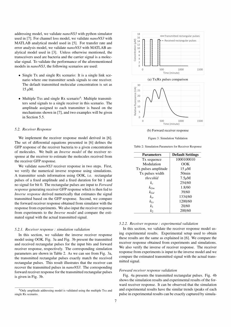
Experimental analysis and verification of BMC networks aretime-consuming [8]. Fig. 3b in Section 5 presents the responseof a receiver bacteria to an input rectangular pulse of AHL sig-nal with concentration 15µM and a pulse width of 50 minutes.It can be observed from Fig. 3b that it takes the receiver bacte-ria few hundred minutes to generate a GFP response and readyto receive next signal. Due to such high processing time andtransmission delays, experimental verification of different algo-rithms is extremely time inefficient. Also, since the receivernodes are live bacteria, it is difficult to replicate parametersacross different experiments. Due to the complexity of exper-imental setup and the time involved, it is difficult to vary dif-ferent parameters like channel characteristics or characteristicsof the transmitted signal. A computer-based BMC simulatoris thus necessary to analyze the performance of the existing orstate-of-the-art algorithms of BMC. The objective of nanoNS3is thus to simulate a BMC network with genetically engineeredbacterial transceivers in a microfluidic environment. Based onthe extensible property of nanoNS3, customized BMC relatedfeatures can also be implemented in nanoNS3.

Implementing a molecular communication simulator withbacteria as transceivers has the following challenges.

1) Due to the dynamic nature of the system, algorithms de-veloped for BMC networks differ from traditional commu-nication algorithms significantly. Implementing state-of-the-art protocols is important and is not a trivial extensionof the traditional communication modules. Transceivers ina BMC network have high processing time and transmis-sion delays, so BMC networks are hence called super-slownetworks [8]. Protocols to improve efficiency of such slow

1The coding style of nanoNS3 follows ns-3 coding style, e.g., the code lay-out of nanoNS3 follows the GNU coding standard layout for C and extends itto C++, and name encoding in nanoNS3 follows the CamelCase convention.

networks differ from traditional communication protocolsin terms of frame structure, dimensions used, and algo-rithms.

2) The response of a bacterial receiver to chemical moleculesinvolves multiple processes [6] and is non-linear. Accu-rate modeling of the receiver response is important to sim-ulate a molecular communication network with bacterialtransceivers. The model in use must be specific to thetransceiver considered. In this work, we focus on the bac-terial communication network and hence an accurate mod-eling of the response of receiver bacteria to an input chem-ical must be used in the simulator.

3) The simulator should have high computational efficiencyin simulating large BMC networks and long packet sizes.

In this context, we have developed nanoNS3 that addressesthe challenges identified in building a BMC network simula-tor. nanoNS3 is developed and validated based on experimentsperformed using genetically engineered bacteria in microfluidicenvironment. nanoNS3 is built on top of ns-3, which is a dis-crete event based simulator. A discrete event based simulator isbest suited for simulating processes with long delays. It tracksthe change in state of events and not the absolute time. Simu-lating absolute time is expensive for super-slow networks likeBMC and therefore, event-based simulations are faster and scal-able. Later in this section, we present simulation time complex-ity of time-based simulator that takes very long time to simulatea molecular communication system.

BMC networks are super-slow networks with very longtransmission delays. Thus, using ns-3 helps nanoNS3 to betime efficient. ns-3 borrows concepts from [17] focusing onbuilding a scalable network simulator, so ns-3 is also equippedwith good scalability performance. Therefore, we choose to de-velop our BMC network simulator on top of ns-3 allowing usto address one of the challenges viz., simulation time efficiencyand simulating large networks. Some of the advantages of us-ing ns-3 are: 1) maintaining good computational efficiency forlarge networks with high payloads, 2) open source and ease ofextensibility which enable users to implement state-of-the-artalgorithms based on users’ demands, 3) with supporting toolsfrom ns-3 that can be utilized directly (e.g. ns-3 logging andtracing systems).

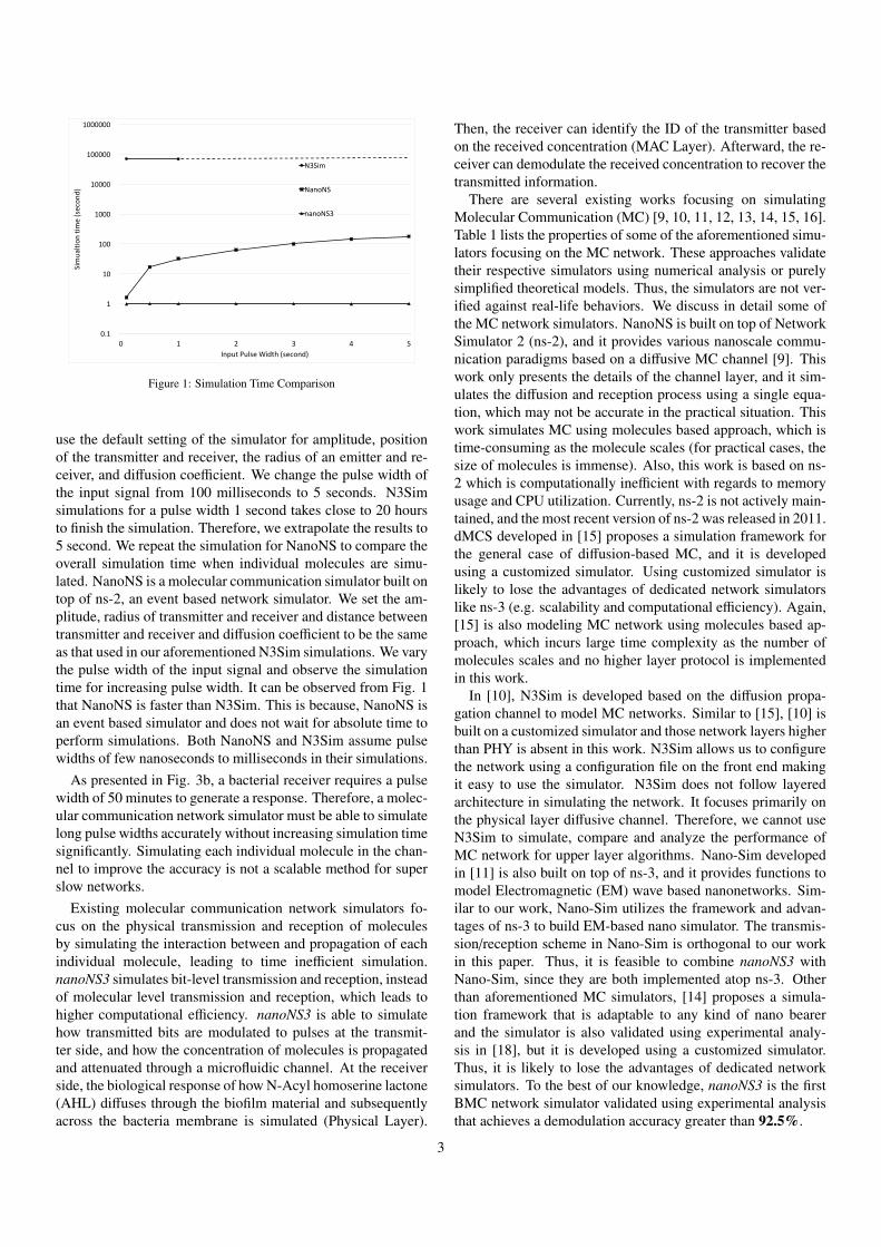
Fig. 1 presents the time to run a simulation for an input sig-nal with pulse duration as x-axis when using molecular com-munication simulators NanoNS, N3Sim and nanoNS32. Y-axis,plotted in logarithmic scale, plots the time for a simulationto run in an OPTIPLEX 9020 desktop computer running In-tel(R) Core(TM) i7-4770 CPU at 3.40GHz and 24GB RAM.The background processes are shut down and we use time com-mand of Linux to calculate the CPU time to run the simulation.We explain in details for some of the existing simulators laterin the section. We implemented OOK in N3Sim and NanoNS.N3Sim is a time-based simulation framework developed to sim-ulate diffusion based molecular communication networks. We

2Details of simulators comparison with nanoNS3 is presented in Table 1.

2

0.1

1

10

100

1000

10000

100000

1000000

0 1 2 3 4 5

Simualtion

time(secon

d)

InputPulseWidth(second)

N3Sim

NanoNS

nanoNS3

Figure 1: Simulation Time Comparison

use the default setting of the simulator for amplitude, positionof the transmitter and receiver, the radius of an emitter and re-ceiver, and diffusion coefficient. We change the pulse width ofthe input signal from 100 milliseconds to 5 seconds. N3Simsimulations for a pulse width 1 second takes close to 20 hoursto finish the simulation. Therefore, we extrapolate the results to5 second. We repeat the simulation for NanoNS to compare theoverall simulation time when individual molecules are simu-lated. NanoNS is a molecular communication simulator built ontop of ns-2, an event based network simulator. We set the am-plitude, radius of transmitter and receiver and distance betweentransmitter and receiver and diffusion coefficient to be the sameas that used in our aforementioned N3Sim simulations. We varythe pulse width of the input signal and observe the simulationtime for increasing pulse width. It can be observed from Fig. 1that NanoNS is faster than N3Sim. This is because, NanoNS isan event based simulator and does not wait for absolute time toperform simulations. Both NanoNS and N3Sim assume pulsewidths of few nanoseconds to milliseconds in their simulations.

As presented in Fig. 3b, a bacterial receiver requires a pulsewidth of 50 minutes to generate a response. Therefore, a molec-ular communication network simulator must be able to simulatelong pulse widths accurately without increasing simulation timesignificantly. Simulating each individual molecule in the chan-nel to improve the accuracy is not a scalable method for superslow networks.

Existing molecular communication network simulators fo-cus on the physical transmission and reception of moleculesby simulating the interaction between and propagation of eachindividual molecule, leading to time inefficient simulation.nanoNS3 simulates bit-level transmission and reception, insteadof molecular level transmission and reception, which leads tohigher computational efficiency. nanoNS3 is able to simulatehow transmitted bits are modulated to pulses at the transmit-ter side, and how the concentration of molecules is propagatedand attenuated through a microfluidic channel. At the receiverside, the biological response of how N-Acyl homoserine lactone(AHL) diffuses through the biofilm material and subsequentlyacross the bacteria membrane is simulated (Physical Layer).

Then, the receiver can identify the ID of the transmitter basedon the received concentration (MAC Layer). Afterward, the re-ceiver can demodulate the received concentration to recover thetransmitted information.

There are several existing works focusing on simulatingMolecular Communication (MC) [9, 10, 11, 12, 13, 14, 15, 16].Table 1 lists the properties of some of the aforementioned simu-lators focusing on the MC network. These approaches validatetheir respective simulators using numerical analysis or purelysimplified theoretical models. Thus, the simulators are not ver-ified against real-life behaviors. We discuss in detail some ofthe MC network simulators. NanoNS is built on top of NetworkSimulator 2 (ns-2), and it provides various nanoscale commu-nication paradigms based on a diffusive MC channel [9]. Thiswork only presents the details of the channel layer, and it sim-ulates the diffusion and reception process using a single equa-tion, which may not be accurate in the practical situation. Thiswork simulates MC using molecules based approach, which istime-consuming as the molecule scales (for practical cases, thesize of molecules is immense). Also, this work is based on ns-2 which is computationally inefficient with regards to memoryusage and CPU utilization. Currently, ns-2 is not actively main-tained, and the most recent version of ns-2 was released in 2011.dMCS developed in [15] proposes a simulation framework forthe general case of diffusion-based MC, and it is developedusing a customized simulator. Using customized simulator islikely to lose the advantages of dedicated network simulatorslike ns-3 (e.g. scalability and computational efficiency). Again,[15] is also modeling MC network using molecules based ap-proach, which incurs large time complexity as the number ofmolecules scales and no higher layer protocol is implementedin this work.

In [10], N3Sim is developed based on the diffusion propa-gation channel to model MC networks. Similar to [15], [10] isbuilt on a customized simulator and those network layers higherthan PHY is absent in this work. N3Sim allows us to configurethe network using a configuration file on the front end makingit easy to use the simulator. N3Sim does not follow layeredarchitecture in simulating the network. It focuses primarily onthe physical layer diffusive channel. Therefore, we cannot useN3Sim to simulate, compare and analyze the performance ofMC network for upper layer algorithms. Nano-Sim developedin [11] is also built on top of ns-3, and it provides functions tomodel Electromagnetic (EM) wave based nanonetworks. Sim-ilar to our work, Nano-Sim utilizes the framework and advan-tages of ns-3 to build EM-based nano simulator. The transmis-sion/reception scheme in Nano-Sim is orthogonal to our workin this paper. Thus, it is feasible to combine nanoNS3 withNano-Sim, since they are both implemented atop ns-3. Otherthan aforementioned MC simulators, [14] proposes a simula-tion framework that is adaptable to any kind of nano bearerand the simulator is also validated using experimental analy-sis in [18], but it is developed using a customized simulator.Thus, it is likely to lose the advantages of dedicated networksimulators. To the best of our knowledge, nanoNS3 is the firstBMC network simulator validated using experimental analysisthat achieves a demodulation accuracy greater than 92.5%.

3

Table 1: Simulators Comparison

Features/Simulator NanoNS N3Sim Nano-Sim nanoNS3

PhysicalLayer/Channel

Model

Diffusive channel,Gillespie model forstochastic reaction

process

Baraff’s algorithmsimulating collision

Spectrum channelmodel

Bacterial receivermodel and channel

loss model

ProtocolsImplemented

Molecular nodeemitting molecules

Emitter types togenerate molecules

pulse trains

Selective andRandom routing,TransparentMAC,SmartMAC, Time

spread OOK

OOK, Sourceaddressing, Error

analysis and transferrate analysis model,

ns-3 applicationlayer

Validation Numerical analysisof models used N/A N/A Experimental

evaluationCompatibility of

Network Simulator ns-2 N/A ns-3 ns-3

Programminglanguage used Tcl, C++ Java C++ C++

Modularity ofNetwork

Architecture

Higher layerprotocols of ns-2 can

be integrated withthe physical layer

Does not haveprovision to

implement higherlayer protocols

Higher layerprotocols of ns-3

Higher layerprotocols of ns-3

3. Network Architecture

nanoNS3 is developed atop ns-3 [19]. ns-3 is a discrete event,open source and widely used network simulator for internet sys-tems, targeted primarily for research and educational use (ns-3is developed in C++ and python). ns-3 is developed based onmodules, and each individual module represents a protocol (e.g.AODV), a technology (e.g. WiFi) or an attribute of networks(e.g. mobility). It enables the easy and convenient upgrade ofsource code and triggers the ease of extensibility in ns-3 by thismodular implementation method. ns-3 is actively maintainedand it is free software and licensed under GNU GPLv2 license.ns-3 has the best overall performance compared with other pop-ular network simulators [20]. E.g. ns-3 has the least memoryusage for large-scale network simulations compared with ns-2,OMNeT++, JiST and SimPy. Implementing nanoNS3 in ns-3 has the following major advantages: 1) open sourced avail-ability and ease of implementation for new algorithms, 2) highcomputational efficiency for large-scale networks, and 3) sup-porting tools from ns-3 can be utilized directly (e.g. ns-3 log-ging and tracing systems).

3.1. nanoNS3 Network ArchitectureThe high-level structure of nanoNS3 is shown in Fig. 2. The

name of seven important classes with the structure of the corre-sponding network layers are given in Fig. 2. The functionalityof each class is discussed briefly below:

• NanoNetDevice: It is similar to the Network InterfaceCard (NIC), and it can support different nano commu-nication technologies (e.g. diffusive or EM wave basednano communication schemes) and corresponding proto-cols (e.g. amplitude addressing).

• NanoNode: It can be regarded as the physical device, anddifferent NanoNetDevices can be integrated with NanoN-ode to provide corresponding communication technolo-gies and protocols to enable NanoNode to communicatewith each other.

• PacketSocket: This class is a simple and original ns-3 ap-plication class, which does not use IP addresses. It is usedto set up user defined applications for nano communica-tions by controlling application-related parameters, e.g.,packet arriving interval, the number of maximal transmis-sion packets and packet size.

• NanoRouting: This class manages message forwarding byeach NanoNode.

• NanoMAC: This class manages channel access of differentNanoNodes, and it also manages MAC layer addressingmechanism.

• NanoPHY: This class is used to simulate the process oftransmitters and receivers to transmit and receive the nanosignals. The corresponding functionality of this class in-cludes modulation, demodulation, error analysis and trans-fer rate analysis, and receiver response.

• NanoChannel: This class is used to set up channel condi-tions, and then the channel loss can be calculated to simu-late how the transmitted signals are propagated and atten-uated in the corresponding microfluidic channel.

Specifically, packet client, packet server, and packet addressare three classes related to packet socket class. The packet

4

Figure 2: nanoNS3 Architecture

client class defines how packets are transmitted from Tx ap-plication layer, and the packet server class defines how pack-ets are received from Rx application layer. The packet addressclass defines how addresses of different nodes are set up. Weintegrate the ns-3 original application class into nanoNS3, in or-der to make it more convenient to integrate other original ns-3classes with nanoNS3, e.g. transport layer protocol. In ns-3,transport layer protocol is integrated with socket, so we inte-grate packet socket into nanoNS3 to make it possible for trans-port layer extension. The parameters for each aforementionedclass can be customized by users. Protocols implemented inNanoMAC, NanoPHY , and NanoChannel will be discussed inSection 4.

4. Protocols Implemented

nanoNS3 implements some of the basic protocols to simulatebacterial molecular communication networks. The important5 models implemented in nanoNS3 are: 1) Receiver responsemodel, 2) Channel loss model, 3) OOK model, 4) Amplitudeaddressing model and 5) Transfer rate and error analysis model.

4.1. Receiver Response ModelAs discussed in Section 2, accurate modeling of receiver re-

sponse is important to simulate BMC networks. nanoNS3 fo-cuses on simulating BMC networks and hence modeling of theresponse of bacteria to molecular signal is described in this sec-tion. The bacterial receiver implemented in this simulator is apopulation of genetically engineered E. coli bacteria that gen-erates a Green Fluorescent Protein (GFP) on receiving AHLmolecules. The transceivers are located in a microfluidic deviceconnected by microfluidic pathways. The transmitter transmitsmolecules that are transported to the receiver through microflu-idic pathways and the receiver emits green fluorescence. Therelative fluorescence of the receiver bacteria indicates the sig-nal received. [6] reviews the existing bacterial receiver models

in a microfluidic environment and proposes a new model. [6]validates the model using experiments. In nanoNS3, we imple-ment the following model proposed in [6].

dAHLi

dt= kc(AHLe − AHLi) − k1AHLi

2LuxR2 + k1C1 (1)

dC1

dt= k1AHLi

2LuxR2 − k1C1 − k2C2PLux (2)

dC2

dt= k2C1PLux − k2C2 − ktrC2 (3)

dLuxRdt

= kLc − 2C1 − 2C2 (4)

dGFPi

dt= ktrC2 − kGmGFPi − kGdGFPi (5)

dGFPm

dt= kGmG + i − kGdGFPm (6)

AHLe and AHLi are the external and internal concentra-tions of molecules at the receiver. LuxR,C1,C2, and GFPi

represent internal parameters of the receiver bacteria. GFPm

represents the concentration of GFP which in turn repre-sents the relative fluorescence at the receiver. Vector k =

[kc, k1, k2, kLc, ktr, kGd, kGm] represents rate constants of the pro-cesses in the receiver. The equations and corresponding deriva-tion are explained in detail in [6].

The above equations are used to model the channel and re-ceiver response in nanoNS3. The transmitter module generatesbits and those bits are input to the modulator. Modulator im-plemented in nanoNS3 is OOK and hence bits are mapped torectangular pulses. The rectangular pulses are input to theseequations to simulate the GFP response of the receiver. A nu-merical inverse of these equations is used to sample and quan-tize the received signal. The output of the sample and quantizemodules is then fed to the demodulator to process. This modelgives a bit level response at the receiver.

4.2. Channel Loss Model

Microfluidic channel loss model is an important componentfor BMC simulators, which provides insights for how the con-centration of signals are attenuated while propagating in mi-crofluidic channel. [5] provides a comprehensive coverage ofthe microfluidic channels with fluid flow for diffusion-basedFlow-induced Molecular Communication (FMC). In FMC, thefluid is flowing through a microfluidic channel and it serves as acommunication channel to connect patches of molecular trans-mitter and receiver, such as bacterial habitat. In [5], an analyticstudy of the propagation of the molecules in the form of theimpulse response is performed incorporating the physical sys-tem parameters. The goal of the propagation loss model is todetermine the channel loss effects caused on the molecular sig-nal with respect to the distance, fluid flow parameters (pressuredrop, flow velocity, microfluidic channel geometry and fluidtype), and type of the molecule (diffusion constant). In [5],channel loss models for the basic microfluidic channel shapes(straight and turning) and cross-sections (rectangular, square,

5

elliptical, circular) are developed incorporating the character-istics of the fluid flow and mass transport in the microfluidicchannels. In nanoNS3, we implement the models presentedin [5]. In the interest of brevity, we will illustrate rectangu-lar cross-section microfluidic channel loss model in this sec-tion, and evaluate the specific microfluidic channel loss modelin Section 5. The governing set of equations for the channelloss in a rectangular microfluidic channel are given as [5].

Grect =h3w12µl

∗ (1 − 0.63hw

) (7)

urect = Grect ∗ 4p (8)

τrect = l/urect (9)

T Frect = e−(k2D+ jkurect)∗τrect (10)

where Grect, urect are the hydraulic conductance of the mi-crofluidic channel and area-averaged flow rate, respectively.Grect is a function of channel cross-section shape, dimensions,and viscosity of the fluid (µ). urect is a function of pressure drop(4p) and Grect. τrect and T Frect are the delay and attenuationof channel, respectively. h and w represent the channel heightand width. l and D are the lengths of the straight channel andTaylor dispersion-adjusted diffusion constant. The detailed ex-planations for all microfluidic channel loss models are given in[5].

4.3. On-Off Keying (OOK) ModelModulation is the process of varying the properties of a sig-

nal to convey the information. Modulation determines the rateof transmission. ns-3 is a packet-level simulator and hence al-lows users to change modulation by changing the transmissionrate. In nanoNS3, we implement bit level simulation and henceimplement a module for modulation that maps each input bit toa signal to be transmitted. OOK is one of the simplest modula-tion techniques and majority of works on BMC assume OOK asthe modulation technique. OOK transmits a rectangular pulseof amplitude/concentration A for a duration of T1 time units tosend bit 1 and no signal for T2 time units to send bit 0. OOKmodule in nanoNS3 generates a rectangular pulse of a givenamplitude and a given duration. Then, the generated rectangu-lar pulse is fed to the channel model.

4.4. Transfer Rate and Error Analysis ModelBased on the framework of nanoNS3, a theoretical analysis

model [3] is implemented in nanoNS3, which is designed to es-timate the theoretical limits of the information transfer rate andcorresponding error probabilities of bacterial molecular com-munication based on the uncertainty of communications, i.e.,transmission, propagation and reception. In [3], this work con-siders a molecular communication setting in which the diffu-sion channel inputs and outputs are OOK with the binary set

{0,

1}. The effects of uncertainty in the production of molecules,

channel parameters and reception process on the overall noiseof the communication are considered. This model can be usedto study the theoretical limits of the information transfer ratein terms of the number of bacteria per node, noise level and

maximum molecule production levels. Also, it can be utilizedto analyze the achievable rates and the error probabilities of M-ary schemes.3 In nanoNS3, we implement the models presentedin [3]. In the interest of brevity, we will not present the descrip-tion of the transmission, propagation and reception model andcorresponding formula proofing.

4.5. Amplitude Addressing ModelThe models mentioned above (receiver response, channel

loss, transfer rate and error analysis and OOK) model the chan-nel and physical layer of BMC networks. A MAC protocolis required in a network with multiple sources to achieve fair-ness and reduce collisions. MAC protocols used in wired orwireless networks as implemented in ns-3 increase the delayand decrease the throughput in a super-slow network like theBMC network. [7] considers a multiple sources and single re-ceiver topology and proposes a MAC protocol to improve theBMC network throughput. Multiple sources transmitting to asingle receiver is a typical sensing network scenario. [7] pro-poses a local addressing mechanism which implicitly performsMAC, and it is implemented in nanoNS3. [7] analyzes the ad-vantages and disadvantages of various addressing mechanismsand proposes Amplitude Addressing for BMC networks. Am-plitude Addressing assigns distinct amplitudes to each user in aBMC network and each user uses the assigned amplitude withOOK to transmit information. The receiver receives the sum ofthe transmitted amplitudes which are then resolved to identifythe individual amplitude thus solving addressing and MAC inthe local network. We further implement two different receiversviz., load-aware and load-unaware. Load-aware receiver has anestimate of input load of the transmitter. Therefore, the decod-ing table (decoding table is used to decode the transmitter IDbased on the received signal) is a function of the input load ofthe transmitter. On the other hand, load-unaware receiver as-sumes that the input is uniformly distributed for the transmitterand the decoding table is fixed. We present the results for boththe receivers in the next section. A global address is requiredto map local address to the source. nanoNS3 does not have aglobal addressing module, but MAC address of ns-3 nodes canbe used as a global address module in simulations

5. Results

In this section, we present the evaluation results of nanoNS3using both simulation-based and experimental-based validationfor the 5 models mentioned in Section 4. nanoNS3 provides twoexamples of scenario setup: 1) single Tx and single Rx, and 2)multiple Txs and single Rx.

5.1. MethodologyIn this section, we validate nanoNS3 with protocols men-

tioned in Section 4. For the receiver response model, we vali-date the simulation results of nanoNS3 with results from MAT-LAB analytic model used in [6] and experiments. For amplitude

3Although nanoNS3 only supports OOK, it can be utilized to study the the-oretical limits of transfer rate and error probability for M-ary schemes.

6

addressing model, we validate nanoNS3 with python simulatorused in [7]. For channel loss model, we validate nanoNS3 withMATLAB analytical model used in [5]. For transfer rate anderror analysis model, we validate nanoNS3 with MATLAB an-alytical model used in [3]. Unless otherwise mentioned, thetransceivers used are bacteria and the carrier signal is a molec-ular signal. To validate the performance of the aforementionedmodels in nanoNS3, the following scenarios are used:

• Single Tx and single Rx scenario: It is a single link sce-nario where one transmitter sends signals to one receiver.The default transmitted molecular concentration is set as15 µM.

• Multiple Txs and single Rx scenario4: Multiple transmit-ters send signals to a single receiver in this scenario. Theamplitude assigned to each transmitter is based on themechanisms shown in [7], and two examples will be givenin Section 5.5.

5.2. Receiver Response

We implement the receiver response model derived in [6].The set of differential equations presented in [6] defines theGFP response of the receiver bacteria to a given concentrationof molecules. We built an Inverse model of the receiver re-sponse at the receiver to estimate the molecules received fromthe receiver GFP response.

We validate nanoNS3 receiver response in two steps. First,we verify the numerical inverse response using simulations.A transmitter sends information using OOK, i.e. rectangularpulses of a fixed amplitude and a fixed duration for bit 1 andno signal for bit 0. The rectangular pulses are input to Forwardresponse generating receiver GFP response which is then fed toInverse response derived numerically that estimates the signaltransmitted based on the GFP response. Second, we comparethe forward receiver response obtained from simulator with theresponse from experiments. We also input the receiver responsefrom experiments to the Inverse model and compare the esti-mated signal with the actual transmitted signal.

5.2.1. Receiver response : simulation validationIn this section, we validate the inverse receiver response

model using OOK. Fig. 3a and Fig. 3b present the transmittedand received rectangular pulses for the input bits and forwardreceiver response, respectively. The corresponding simulationparameters are shown in Table 2. As we can see from Fig. 3a,the transmitted rectangular pulses exactly match the receivedrectangular pulses. This result illustrates that the receiver canrecover the transmitted pulses in nanoNS3. The correspondingforward receiver response for the transmitted rectangular pulsesis given in Fig. 3b.

4Only amplitude addressing model is validated using the multiple Txs andsingle Rx scenario.

0 500 1000 150002468

1012141618

Time (minute)

Concen

tration

(μM) Transmitted rectangular pulses

Received rectangular pulses

(a) Tx/Rx pulses comparison

0 500 1000 150005

1015202530

Time (minute)

Relativ

e fluore

sence (

UA)(b) Forward receiver response

Figure 3: Simulation Validation

Table 2: Simulation Parameters for Receiver Response

Parameters Default SettingsTx sequence 1000100010Modulation OOK

Tx pulses amplitude 15 µMTx pulses width 50min

threshld 7.5µMkc 254/60

kGm 1.8/60kGd 39/60ktr 1334/60kLc 1200/60k1 20/60k2 200/60

5.2.2. Receiver response : experimental validationIn this section, we validate the receiver response model us-

ing experimental results. Experimental setup used to obtainthese results are the same as explained in [6]. We compare thereceiver response obtained from experiments and simulations.We also verify the inverse of receiver response. The receiverresponse from experiments is input to the inverse model and wecompare the estimated transmitted signal with the actual trans-mitted signal.

Forward receiver response validationFig. 4a presents the transmitted rectangular pulses. Fig. 4b

shows the simulation results and experimental results of the for-ward receiver response. It can be observed that the simulationand experimental results have the similar trends (peaks of eachpulse in experimental results can be exactly captured by simula-

7

05

101520

0 500 1000 1500

Consen

tration

(μM)

Time (minute)

(a) Experimental Tx pulses

05

1015202530

0 500 1000 1500

Relativ

e fluore

sence (

AU)

Time (minute)

Experimental validationSimulation

(b) Forward receiver response

Figure 4: Experimental Validation

tion). Four different Tx sequences with 10 bits in each sequenceare set as Tx sequence in the experimental apparatus, and eachof them shows the similar trend as the presented results.

Inverse receiver response validationBased on the experimental results of forward receiver re-

sponse, we validated the inverse of the receiver response. FromFig. 4b, it is clear that experimental results of forward receiverresponse are not as smooth as the simulation results of forwardreceiver response. In order to get rid of noises and system er-rors, we use Loess smooth function (with 10% span) in MAT-LAB to smooth the experimental results. The correspondingexperimental results are shown in Fig. 5a. Then, we inputthose smoothed experimental results to the inverse of receiverresponse model in nanoNS3, and we succeeded to recover thetransmitted bits at the receiver side. From Fig. 5b, it can be ob-served that the peaks of transmitted and received pulses matchwith each other. In order to demodulate the received pulses,we calculate the average concentration for the pulse duration ofeach bit, where average concentration for bit i is represented asAvei. We set a threshold to determine the bit level, where thethreshold is set as half of transmitted concentration. Receivedbit is determined by the following equation:

Received bit =

1 if Avei >= threshold0 if Avei < threshold

Utilizing this method, we can achieve 100% of demodulationrate for the presented case of experimental results. The averagedemodulation rate of four sets of experimental results achieves92.5%.

05

1015202530

0 500 1000 1500

Relativ

e fluore

sence (

AU)

Time (minute)

Experimental validationSimulation

(a) Processed experimental results

05

101520

0 500 1000 1500

Consen

tration

(μM)

Time (minute)

Transmitted rectangular pulsesReceived rectangular pulses

(b) Processed experimental results validation

Figure 5: Experimental Validation

To conclude, nanoNS3 provides an experimental-based re-ceiver response model:

For the receiver response model, the simulation re-sults of nanoNS3 match the simulation results ofMATLAB analytic model. The implemented model en-ables higher layer protocols in nanoNS3 to achievehigh accuracy of their simulation performance.

5.3. Channel Loss

In this section, we compare the channel loss model in singleTx and single Rx scenario. We compare the results obtainedby nanoNS3 with respect to the MATLAB using the describedanalytic channel loss model in Section 4.2. The objective is toshow that the numerical results of nanoNS3 match the numeri-cal results from MATLAB for the analytic model channel lossmodel. The details of the default parameter settings are shownin Table 3.

Fig. 6a and 6b illustrate how the impulse response attenua-tion of straight and turning channel varies with frequency (ra-dians per meter), respectively. We observe that the channel lossmodule implemented in nanoNS3 provides the exactly same re-sults with the analytic model evaluation in MATLAB for bothFig. 6a and 6b.

To conclude, nanoNS3 provides a microfluidic channel lossmodel:

The simulation results of nanoNS3 match the simula-tion results of MATLAB analytic model. More channelproperties and other channel loss model can be easilyimplemented in nanoNS3 based on the implementedchannel loss model.

8

Table 3: Simulation Parameters for Channel Loss

Parameters Default SettingsChannel shape rectangularTurning angle 30 degree

viscosity 10−3Pa*sD 10 ∗ 10−10m2/s4p 500 pal 10mmh 6µmw 25µm

00.20.40.60.8

1

0 5000 10000 15000

Attenua

tion

k (radians per meter)

nanoNS3Matlab analytic model

(a) Straight rectangular channel

00.20.40.60.8

1

0 5000 10000 15000 20000 25000

Attenua

tion

k (radians per meter)

nanoNS3Matlab analytic model

(b) Turning rectangular channel

Figure 6: Channel loss validation

Table 4: Simulation Parameters for Capacity and Error Analysis

Parameters Default SettingsNumber of bacterial 100

Number of ligand receptors 50Square of combined noise variance 0.1

M-ary scheme 16

5.4. Transfer Rate and Error Analysis

In this section, we compare the transfer rate and error anal-ysis model in single Tx and single Rx scenario. We comparethe results obtained by nanoNS3 with respect to the MATLABanalytic model used in [3]. The objective is to show that thenumerical results of nanoNS3 match the numerical results fromMATLAB analytic model. The details of the default parametersettings are shown in Table 4.

Fig. 7 illustrates how the channel capacity varies with themaximum concentration of molecules. As M-ary scheme is uti-lized, Fig. 8a and 8b illustrate how the channel capacity andcorresponding error rate varies with the maximum concentra-

0

1

2

3

4

5

6

7

0 200 400 600

Cap

acit

y (b

it/c

han

nel

use

)

Amax (nM)

Matlab analytic model

nanons3

Figure 7: Transfer Rate Analysis

0

1

2

3

4

5

0 100 200 300 400

Info

rmat

ion

Rat

e (b

its/

sam

ple

)

Amax (nM)

Matlab analytic model

nanoNS3

(a) Transfer Rate Analysis

0

0.01

0.02

0.03

0.04

0.05

0.06

0.07

0.08

0 100 200 300 400

Erro

r P

rob

abili

ty

Amax (nM)

Matlab analytic model

nanoNS3

(b) Error Rate Analysis

Figure 8: Transfer Rate and Error Rate Analysis for Corresponding Modulation

tion of molecules. We observe that the theoretical limits forboth capacity and error rate generated from nanoNS3 match theresults with the MATLAB analytic model from Fig. 7, Fig. 8aand 8b.

To conclude, nanoNS3 provides a theoretical analysis model:

The simulation results of nanoNS3 match the simula-tion results of the MATLAB analytic model. Based onthe implemented theoretical analysis model, transferrate and error probability with corresponding modu-lations can be estimated.

5.5. Amplitude Addressing

In this section, we validate the amplitude addressing mech-anism in multiple Txs and single Rx scenario. We comparethe performance of nanoNS3 versus the custom built pythonsimulator used in [7]. The objective is to show that the sim-ulation results of nanoNS3 match the simulation results fromthe aforementioned python simulator. The details of default pa-

9

Table 5: Simulation Parameters for Amplitude Addressing

Parameters Default SettingsNumber of Tx bits 100

Amplitude assignment mechanism Integer/BinaryTx pulses width 50mins

Tx pulses interval 20minspt 0.5

Max amplitude 15µMNumber of Tx users 5

rameter settings are shown in Table 5. Two examples of am-plitude assignment mechanism will be briefly introduced. Forinteger amplitude assignment mechanism, each user is assignedwith a unique amplitude based on the node ID. E.g. amplitudes{1,2,3} are assigned to transmitters with ID {1,2,3} with one-to-one correspondence. For binary amplitude assignment mecha-nism, amplitudes {1,2,4,8} are assigned to transmitters with ID{1,2,3,4} with one-to-one correspondence.

Fig. 9a plots the demodulation accuracy for load unaware ad-dressing at the receiver for varying input load for integer ampli-tude assignment. As we can see from Fig. 9a, the performanceof nanoNS3 is very close to that of the custom built python sim-ulator used in [7]. Fig. 9b plots the decoding accuracy at thereceiver for varying input load using binary amplitude assign-ment. It can be observed that the simulation results of nanoNS3and the python simulator are very close to each other.

We also compare the performance of load aware and loadunaware receiver. Fig. 10 shows the correct demodulation rateusing load aware and load unaware receiver with binary ampli-tude assignment. It can be observed that when the receiver isaware of the load of the transmitter, correct demodulation rateincreases compared with load unaware receiver. The amplitudesequences used for evaluation are described in detail in [7].

To conclude, nanoNS3 provides an amplitude addressingmechanism:

The simulation results of nanoNS3 match the simu-lation results of the python simulator. Based on theimplemented addressing model, the performance ofhigher layer protocols can be explored (e.g. routingmechanisms).

5.6. Simulator time complexity comparisonIn Section 2, we presented the simulation time complexity of

three simulators NanoNS, N3Sim, and nanoNS3 for increasingsimulation input pulse width. We observed that a time-basedsimulator like N3Sim that simulates molecular interaction isnot suitable for long simulations. The simulation time com-plexity is in the order of hours for input signal duration of fewmilliseconds and is not suitable for long simulations. NanoNSimproves simulation time by using an event-based simulatorlike ns-2 and simplifying molecular interactions. Using sim-ple equations to represent molecular interactions can affect theaccuracy of response of a receiver to an input signal. Simula-tion time complexity of NanoNS increases exponentially withinput pulse width making it unsuitable for longer packet sizes.

00.10.20.30.40.50.60.70.8

5 6 7 8 9 10 11 12

Correc

t demo

dulatio

n rate

Number of Tx users

python simulatornanoNS3

(a) Integer Tx sequence

00.20.40.60.8

1

0.1 0.2 0.3 0.4 0.5 0.6 0.7 0.8 0.9

Correct

demodu

lation

rate

Probability of transmission bit 1 (Pt)

nanoNS3python simulator

(b) Binary Tx sequence

Figure 9: Amplitude Addressing Validation

0

0.2

0.4

0.6

0.8

1

0 0.2 0.4 0.6 0.8 1

Co

rrec

t d

emo

du

lati

on

rat

e

Probability of transmitting bit 1 (Pt)

Load aware

Load unaware

Figure 10: Load unaware vs. load aware receiver

nanoNS3 uses experimentally verified physical layer models tosimulate the response of a receiver to an input signal withoutcompromising on the accuracy of the receiver. nanoNS3 is im-plemented on top of ns-3, an event based, time efficient simula-tor. We compare the simulation time performance of other ex-isting simulators with that of nanoNS3. As expected, nanoNS3has a constant time complexity for increasing pulse width asit uses a bit-level model to simulate bit-level response of re-ceiver bacteria. Constant simulation time complexity makesnanoNS3 suitable for simulating large MC networks with longpulse widths and long packet sizes.

6. Conclusions

In this paper, we describe nanoNS3, a new network simula-tor built atop ns-3 for BMC networks. The choice of the ns-3simulator allows high computational efficiency for large-scalenetworks and easy implementation of new algorithms. An accu-rate model of the bacterial receiver response to chemical signals

10

modulated using OOK is implemented. A microfluidic channelloss model that incorporates the physical system parameters isimplemented in nanoNS3. A source addressing protocol thatimplicitly solves MAC issues is also implemented in nanoNS3.nanoNS3 thus focuses on the channel, PHY and MAC layersof the network protocol stack. Due to the lack of upper layerprotocols in BMC network, nanoNS3 only provides an originalns-3 application layer model for upper layers. By making useof the layered architecture of ns-3, it is possible to use exist-ing IP, transport and application layer protocols in ns-3 to testthe performance of BMC networks. For future work, we planto improve the completeness of nanoNS3 by implementing newfeatures such as channel propagation delay model. Moreover,we will explore merging nanoNS3 with other MC simulatorsthat are also implemented atop ns-3, in order to move closer tothe vision of a general purpose MC simulator.

References

[1] T. Charrier, C. Chapeau, L. Bendria, P. Picart, P. Daniel, G. Thouand, Amulti-channel bioluminescent bacterial biosensor for the on-line detectionof metals and toxicity. part ii: technical development and proof of conceptof the biosensor, Analytical and Bioanalytical Chemistry 400 (4) (2011)1061–1070.

[2] J. Stocker, D. Balluch, M. Gsell, H. Harms, J. Feliciano, S. Daunert,K. A. Malik, J. R. van der Meer, Development of a set of simple bac-terial biosensors for quantitative and rapid measurements of arsenite andarsenate in potable water, Environmental Science & Technology 37 (20)(2003) 4743–4750.

[3] A. Einolghozati, M. Sardari, F. Fekri, Design and analysis of wirelesscommunication systems using diffusion-based molecular communicationamong bacteria, IEEE Transactions on Wireless Communications 12 (12)(2013) 6096–6105.

[4] M. Pierobon, I. F. Akyildiz, A statistical–physical model of interferencein diffusion-based molecular nanonetworks, IEEE Transactions on Com-munications 62 (6) (2014) 2085–2095.

[5] A. O. Bicen, I. F. Akyildiz, System-theoretic analysis and least-squaresdesign of microfluidic channels for flow-induced molecular communica-tion, IEEE Transactions on Signal Processing 61 (20) (2013) 5000–5013.

[6] C. M. Austin, W. Stoy, P. Su, M. C. Harber, J. P. Bardill, B. K. Hammer,C. R. Forest, Modeling and validation of autoinducer-mediated bacte-rial gene expression in microfluidic environments, Biomicrofluidics 8 (3)(2014) art. no. 034116.

[7] B. Krishnaswamy, R. Sivakumar, Source addressing and medium accesscontrol in bacterial communication networks, 2nd ACM Annual Interna-tional Conference on Nanoscale Computing and Communication (2015)1–6.

[8] B. Krishnaswamy, C. M. Austin, J. P. Bardill, D. Russakow, G. L. Holst,B. K. Hammer, C. R. Forest, R. Sivakumar, Time-elapse communication:Bacterial communication on a microfluidic chip, IEEE Transactions onCommunications 61 (12) (2013) 5139–5151.

[9] E. Gul, B. Atakan, O. B. Akan, Nanons: A nanoscale network simu-lator framework for molecular communications, Nano CommunicationNetworks 1 (2) (2010) 138–156.

[10] I. Llatser, D. Demiray, A. Cabellos-Aparicio, D. T. Altilar, E. Alarcon,N3sim: Simulation framework for diffusion-based molecular commu-nication nanonetworks, Simulation Modelling Practice and Theory 42(2014) 210–222.

[11] G. Piro, L. A. Grieco, G. Boggia, P. Camarda, Nano-sim: simulatingelectromagnetic-based nanonetworks in the network simulator 3, 6th In-ternational ICST Conference on Simulation Tools and Techniques (2013)203–210.

[12] Calcomsim: https://sites.google.com/site/calcomsimulator/.[13] Comsol-multiphysics: https://www.comsol.com/comsol-multiphysics.[14] L. Felicetti, M. Femminella, G. Reali, A simulation tool for nanoscale

biological networks, Nano Communication Networks 3 (1) (2012) 2–18.

[15] A. Akkaya, T. Tugcu, dmcs: distributed molecular communication sim-ulator, in: 8th ICST International Conference on Body Area Networks,2013, pp. 468–471.

[16] Y. Jian, B. Krishnaswamy, C. M. Austin, A. O. Bicen, J. E. Perdomo,S. C. Patel, I. F. Akyildiz, C. R. Forest, R. Sivakumar, nanons3: Simulat-ing bacterial molecular communication based nanonetworks in networksimulator 3, 3rd ACM International Conference on Nanoscale Comput-ing and Communication (2016) 17–23.

[17] R. M. Fujimoto, K. Perumalla, A. Park, H. Wu, M. H. Ammar, G. F. Riley,Large-scale network simulation: how big? how fast?, 11th IEEE/ACMInternational Symposium on Modeling, Analysis and Simulation of Com-puter Telecommunications Systems (2003) 116–123.

[18] L. Felicetti, M. Femminella, G. Reali, P. Gresele, M. Malvestiti, J. N.Daigle, Modeling cd40-based molecular communications in blood ves-sels, IEEE Transactions on Nanobioscience 13 (3) (2014) 230–243.

[19] Network simulator 3 : https://www.nsnam.org/.[20] E. Weingartner, H. Vom Lehn, K. Wehrle, A performance comparison of

recent network simulators, IEEE International Conference on Communi-cations (2009) 1–5.

11