NAASC Charlottesville –08 Sep 2011 1 S. T. Myers Interferometric Imaging in CASA An Introduction...
39
1 S. T. Myers NAASC Charlottesville –08 Sep 2011 Interferometric Imaging in CASA An Introduction for ALMA reduction Steven T. Myers National Radio Astronomy Observatory Socorro, NM
-
Upload
leslie-richards -
Category
Documents
-
view
215 -
download
2
Transcript of NAASC Charlottesville –08 Sep 2011 1 S. T. Myers Interferometric Imaging in CASA An Introduction...
1 S. T. Myers NAASC Charlottesville –08 Sep 2011
Interferometric Imaging in CASAAn Introduction for ALMA reduction
Steven T. Myers
National Radio Astronomy Observatory
Socorro, NM
2 S. T. Myers NAASC Charlottesville –08 Sep 2011
Radio Interferometric
Imagingin theory…
3NAASC Charlottesville - 08 Sep 2011
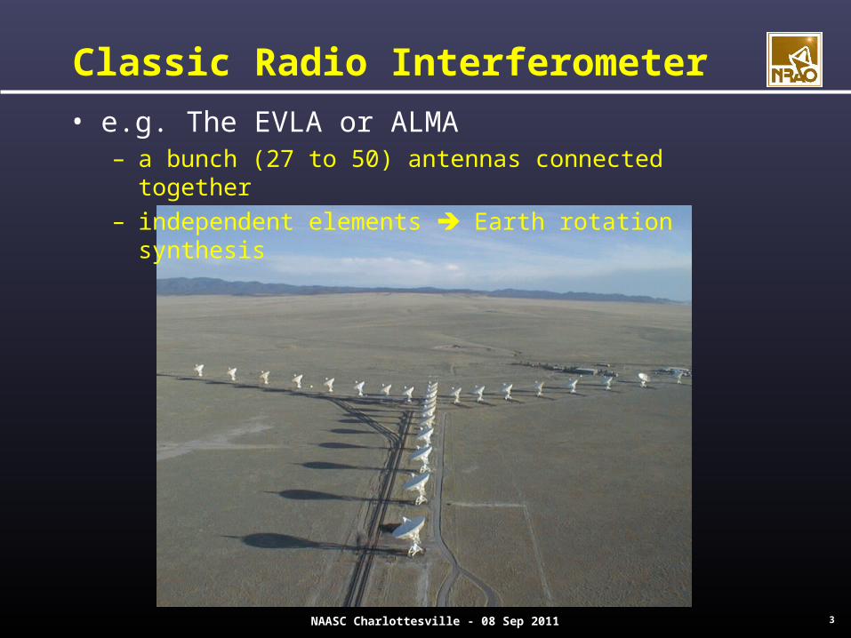
Classic Radio Interferometer
• e.g. The EVLA or ALMA– a bunch (27 to 50) antennas connected together– independent elements Earth rotation synthesis
4NAASC Charlottesville - 08 Sep 2011
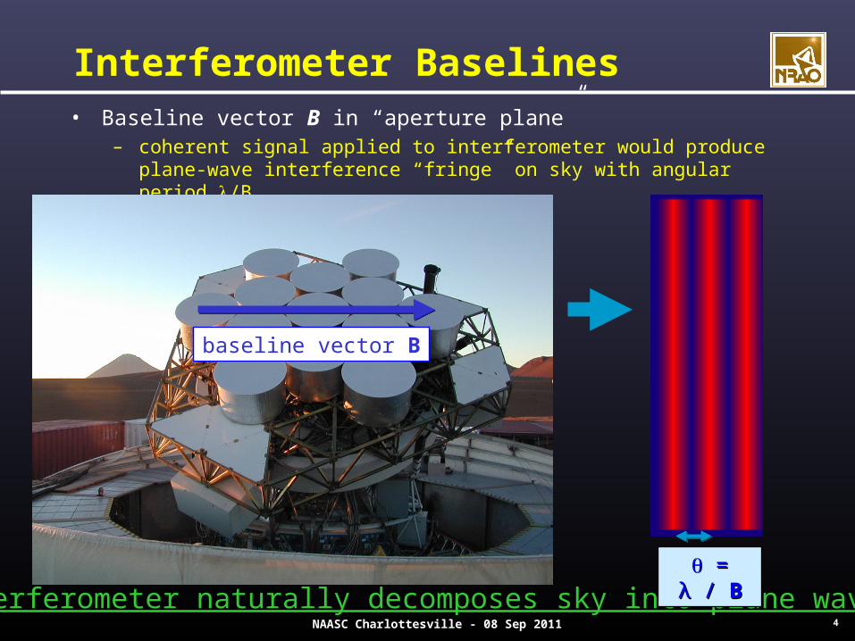
Interferometer Baselines• Baseline vector B in “aperture plane”
– coherent signal applied to interferometer would produce plane-wave interference “fringe” on sky with angular period /B
baseline vector B
interferometer naturally decomposes sky into plane waves! = = λ λ // BB
5NAASC Charlottesville - 08 Sep 2011
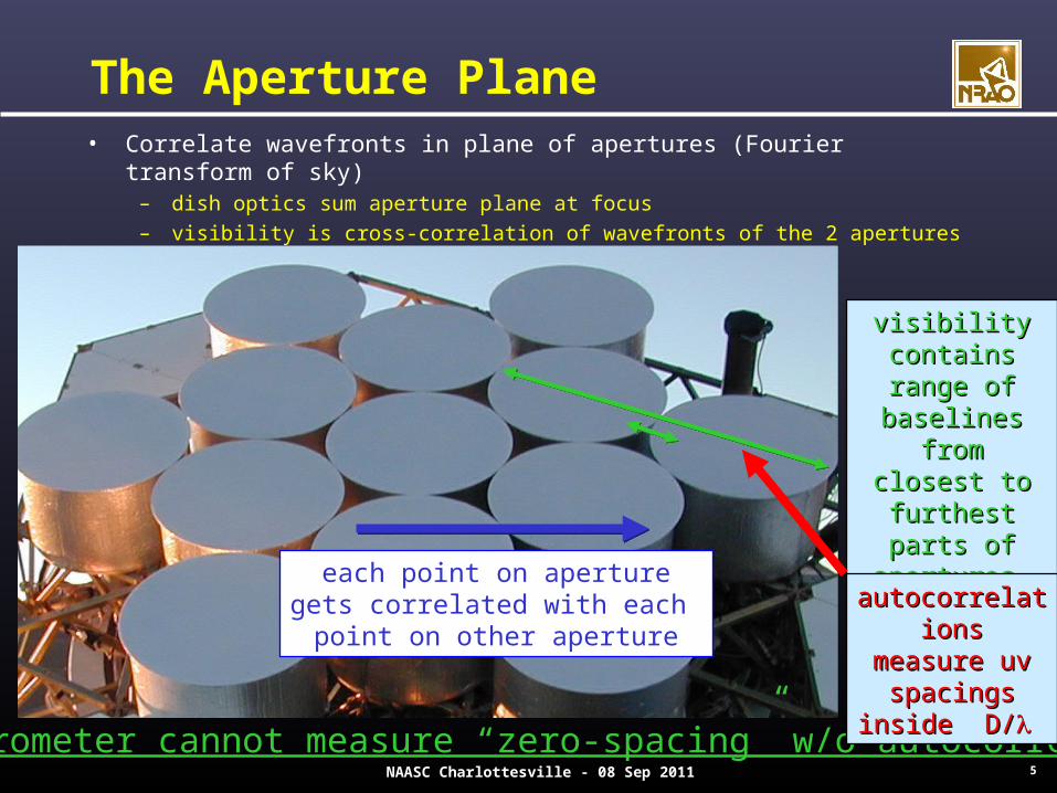
The Aperture Plane• Correlate wavefronts in plane of apertures (Fourier transform of sky)
– dish optics sum aperture plane at focus
– visibility is cross-correlation of wavefronts of the 2 apertures
each point on aperturegets correlated with each
point on other aperture
interferometer cannot measure “zero-spacing” w/o autocorrelations
visibility visibility contains range contains range
of baselines of baselines fromfrom
closest to closest to furthest parts of furthest parts of
apertures apertures
autocorrelationsautocorrelationsmeasure uv measure uv
spacings inside spacings inside D/D/
6NAASC Charlottesville - 08 Sep 2011
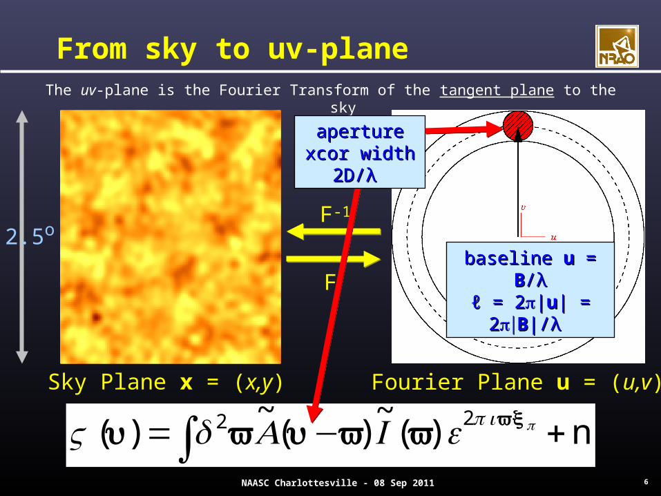
n)(~
)(~
)( 22 +−=∫ ⋅ pieIAdV xvvvuvu π
From sky to uv-planeThe uv-plane is the Fourier Transform of the tangent plane to the sky
Fourier Plane u = (u,v)
baseline baseline uu = = BB//λλℓℓ = 2= 2ππ||uu|| = 2= 2ππBB|/|/λ λ
2.5oF-1
F
Sky Plane x = (x,y)
aperture xcor aperture xcor width 2D/width 2D/λλ
7 S. T. Myers NAASC Charlottesville –08 Sep 2011
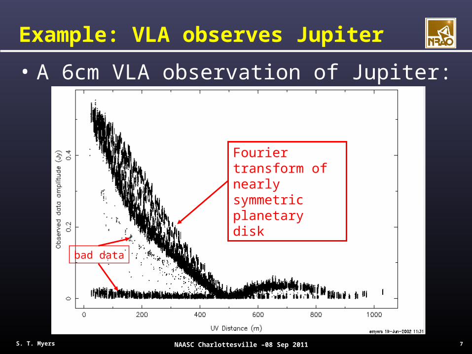
Example: VLA observes Jupiter
• A 6cm VLA observation of Jupiter:
Fourier transform of nearly symmetric planetary disk
bad data
8 S. T. Myers NAASC Charlottesville –08 Sep 2011
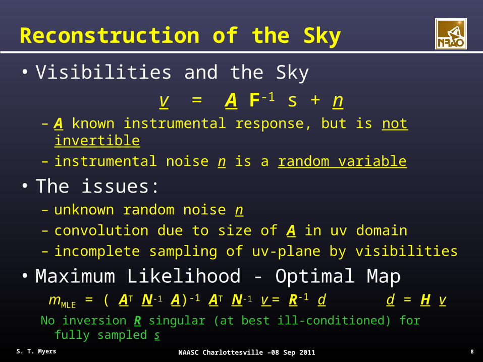
Reconstruction of the Sky
• Visibilities and the Sky
v = A F-1 s + n– A known instrumental response, but is not invertible– instrumental noise n is a random variable
• The issues:– unknown random noise n – convolution due to size of A in uv domain– incomplete sampling of uv-plane by visibilities
• Maximum Likelihood - Optimal MapmMLE = ( AT N-1 A)-1 AT N-1 v = R-1 d d = H v
No inversion R singular (at best ill-conditioned) for fully sampled s
9 S. T. Myers NAASC Charlottesville –08 Sep 2011
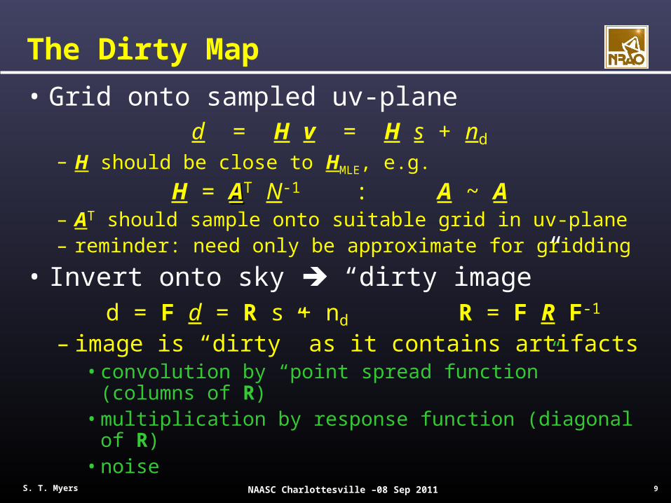
The Dirty Map
• Grid onto sampled uv-planed = H v = H s + nd
– H should be close to HMLE, e.g.
H = AAT N-1 : A ~ A – AT should sample onto suitable grid in uv-plane– reminder: need only be approximate for gridding
• Invert onto sky “dirty image”d = F d = R s + nd R = F R F-1
– image is “dirty” as it contains artifacts• convolution by “point spread function” (columns of R)• multiplication by response function (diagonal of R)• noise
10 S. T. Myers NAASC Charlottesville –08 Sep 2011
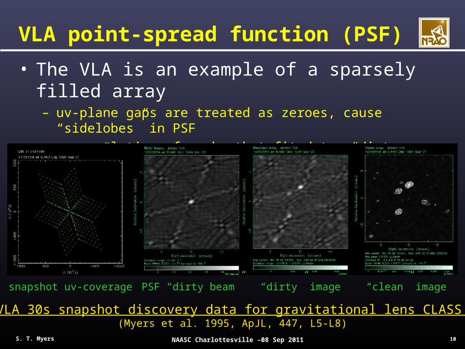
VLA point-spread function (PSF)
• The VLA is an example of a sparsely filled array– uv-plane gaps are treated as zeroes, cause “sidelobes” in PSF– many solutions for sky that fit data, “dirty image” is principal solution– must use “deconvolution” techniques to “clean” image
snapshot uv-coverage
Example: VLA 30s snapshot discovery data for gravitational lens CLASS B1608+656(Myers et al. 1995, ApJL, 447, L5-L8)
PSF “dirty beam” “dirty” image “clean” image
11 S. T. Myers NAASC Charlottesville –08 Sep 2011
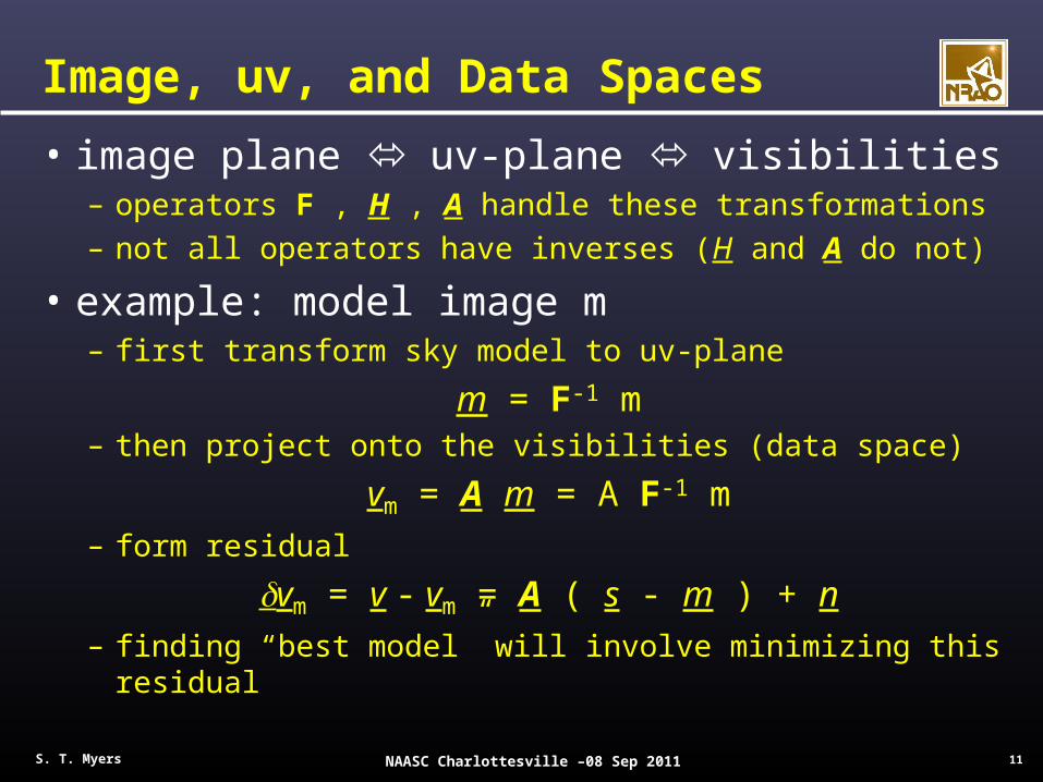
Image, uv, and Data Spaces
• image plane uv-plane visibilities– operators F , H , A handle these transformations– not all operators have inverses (H and A do not)
• example: model image m – first transform sky model to uv-plane
m = F-1 m– then project onto the visibilities (data space)
vm = A m = A F-1 m– form residual
vm = v - vm = A ( s - m ) + n– finding “best model” will involve minimizing this residual

12 S. T. Myers NAASC Charlottesville –08 Sep 2011
Classic Deconvolution
• uv-plane CLEAN algorithm (“major cycles”)– iterate on residual images removing point models
– initial residual data, and model: v0 = v m0 = 0
– form dirty image: d0 = F H v0
– locate peak and residual and put fraction f into model
m1 = f M d0 mask M : 1 at max, else 0
– increment model: m1 = m0 + m1
– form cumulative visibilities and residual
v1 = A m1 = A F-1 m1 v1 = v – v1
– form new dirty residual image: d1 = F H v1
– and repeat until final residual image df is noise-like
13 S. T. Myers NAASC Charlottesville –08 Sep 2011
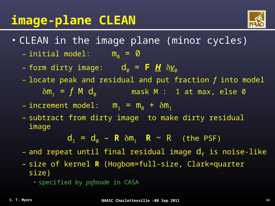
image-plane CLEAN
• CLEAN in the image plane (minor cycles)– initial model: m0 = 0
– form dirty image: d0 = F H v0
– locate peak and residual and put fraction f into model
m1 = f M d0 mask M : 1 at max, else 0
– increment model: m1 = m0 + m1
– subtract from dirty image to make dirty residual image
d1 = d0 – RR m1 RR ~ R (the PSF)
– and repeat until final residual image df is noise-like
– size of kernel RR (Hogbom=full-size, Clark=quarter size)• specified by psfmode in CASA
14 S. T. Myers NAASC Charlottesville –08 Sep 2011
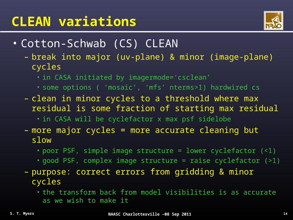
CLEAN variations
• Cotton-Schwab (CS) CLEAN– break into major (uv-plane) & minor (image-plane) cycles
• in CASA initiated by imagermode=‘csclean’• some options ( ‘mosaic’, ‘mfs’ nterms>1) hardwired cs
– clean in minor cycles to a threshold where max residual is some fraction of starting max residual
• in CASA will be cyclefactor x max psf sidelobe
– more major cycles = more accurate cleaning but slow• poor PSF, simple image structure = lower cyclefactor (<1)• good PSF, complex image structure = raise cyclefactor (>1)
– purpose: correct errors from gridding & minor cycles• the transform back from model visibilities is as accurate as we
wish to make it
15 S. T. Myers NAASC Charlottesville –08 Sep 2011
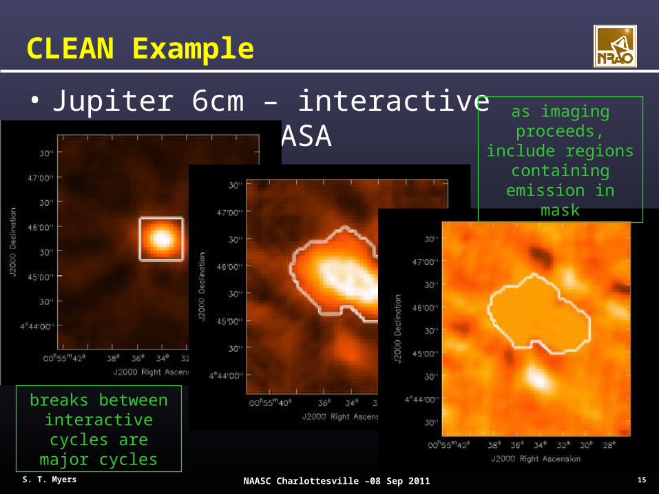
CLEAN Example
• Jupiter 6cm – interactive cleaning in CASAas imaging
proceeds, include regions containing emission in mask
breaks between interactive cycles are major cycles
16 S. T. Myers NAASC Charlottesville –08 Sep 2011
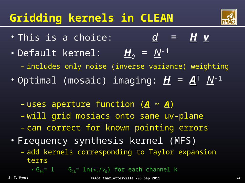
Gridding kernels in CLEAN
• This is a choice: d = H v
• Default kernel: H0 = N-1
– includes only noise (inverse variance) weighting
• Optimal (mosaic) imaging: H = AAT N-1
– uses aperture function (A ~ A)– will grid mosiacs onto same uv-plane– can correct for known pointing errors
• Frequency synthesis kernel (MFS)– add kernels corresponding to Taylor expansion terms
• G0k= 1 G1k= ln(k/0) for each channel k
17 S. T. Myers NAASC Charlottesville –08 Sep 2011
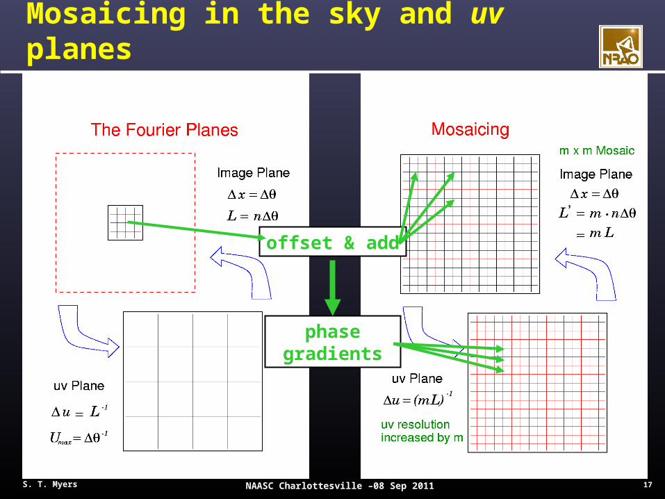
Mosaicing in the sky and uv planes
offset & add
phase gradients
18 S. T. Myers NAASC Charlottesville –08 Sep 2011
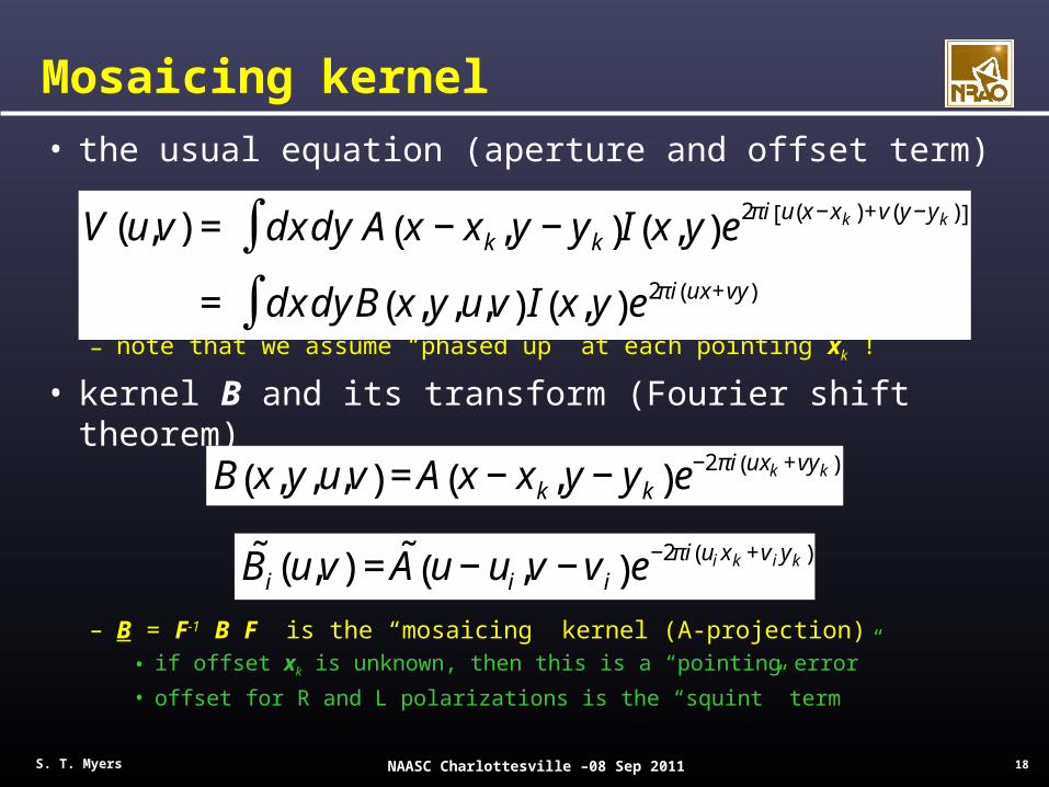
Mosaicing kernel
• the usual equation (aperture and offset term)
– note that we assume “phased up” at each pointing xk !
• kernel B and its transform (Fourier shift theorem)
– B = F-1 B F is the “mosaicing” kernel (A-projection)• if offset xk is unknown, then this is a “pointing error”
• offset for R and L polarizations is the “squint” term
€
V (u,v) = dx dy∫ A x − xk, y − yk( )I x,y( )e2πi u x −xk( )+v y −yk( )[ ]
= dx dy B x, y,u,v( ) I x,y( )∫ e2πi ux +vy( )
€
B x, y,u,v( ) = A x − xk,y − yk( )e−2πi uxk +vyk( )
€
˜ B i u,v( ) = ˜ A u − ui,v − v i( )e−2πi ui xk +vi yk( )
19 S. T. Myers NAASC Charlottesville –08 Sep 2011
Mosaicing considerations
• In CASA, imagermode=‘mosaic’– ftmachine=‘mosaic’ uses A-projection kernel
• grids to single uv-plane, optimally weights fields, most efficient• can be some aliasing, keep mosaic to inner quarter of imsize
– ftmachine=‘ft’ does standard image-plane shift+add• takes much longer, not recommended
– mosaic uses csclean, watch cyclefactor– uses approximate single PSF for entire mosaic
• will “correct” in major cycles
– uses POINTING table when present (FIELD for phases)
• Outputs– standard: .image, .model, .psf– .flux (PB plus weights plus extra PB from A-convolution)– .flux.pbcoverage (just the PB effects)– e.g. to correct to flux on-sky use .image/.flux
20 S. T. Myers NAASC Charlottesville –08 Sep 2011
MEM and CLEAN
• CLEAN– algorithm: find peak in residual image; add fraction to
model; form new residual data & residual image; iterate– performance: good on compact emission, difficult for
extended
• Maximum Entropy Method (MEM)– algorithm: for pixel values p : maximize entropy - p ln p ;
minimize 2(p) to encourage “smooth” extended emission– performance: complicated, suppresses spiky emission, but
fast
• CLEAN and MEM use point (pixel) basis– complete basis – unique representation of image
21 S. T. Myers NAASC Charlottesville –08 Sep 2011
Sparse Approximation Imaging
• Problem: find a model to represent the sky as efficiently as possible, subject to the data constraints and within the noise uncertainty, possibly also subject to prior constraints.– some problems (like ours) cannot be efficiently
reconstructed using orthonormal bases (like pixels or Fourier modes)
– extensive literature on this!– use non-orthogonal bases: multiscale (e.g. Gaussians)– choose dictionary of model elements (atoms)– efficiency: find a representation that uses the fewest number
of atoms
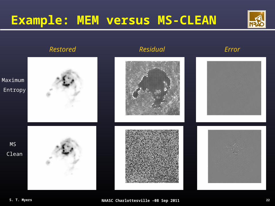
22 S. T. Myers NAASC Charlottesville –08 Sep 2011
Maximum
Entropy
MS
Clean
Restored ErrorResidual
Example: MEM versus MS-CLEAN
23 S. T. Myers NAASC Charlottesville –08 Sep 2011
The Future of Multiscale Methods
• Algorithms– mostly iterative, starting from a blank model– “greedy” methods make locally optimal choices at each step
• MS-CLEAN is a greedy algorithm in this class!– dictionary of points and Gaussians on different scales– is essentially a “Matching Pursuit” (MP) algorithm (e.g.
Tropp 2004)
• Key Research Area in CASA– new arrays are designed for high dynamic range & fidelity– we need efficient, robust, and accurate multiscale methods– integrate multiscale (MS) with multispectral (MFS)
24 S. T. Myers NAASC Charlottesville –08 Sep 2011
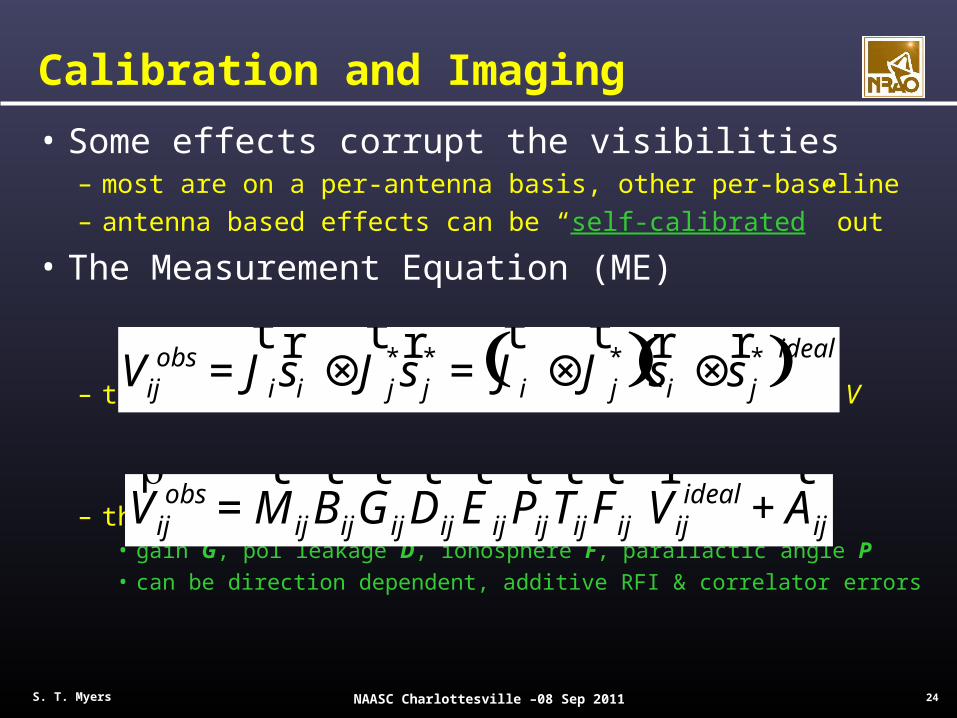
Calibration and Imaging
• Some effects corrupt the visibilities– most are on a per-antenna basis, other per-baseline– antenna based effects can be “self-calibrated” out
• The Measurement Equation (ME)
– the Jones matrices J contain the corruptions to V
– there are different corruption terms to the J • gain G, pol leakage D, ionosphere F, parallactic angle P• can be direction dependent, additive RFI & correlator errors
( )( )ideal
jijijjiiobs
ij ssJJsJsJV **** rrttrtrt⊗⊗=⊗=
€
rV ij
obs =t
M ijt B ij
t G ij
t D ij
t E ij
t P ij
t T ij
t F ij
r V ij
ideal +t A ij
25 S. T. Myers NAASC Charlottesville –08 Sep 2011
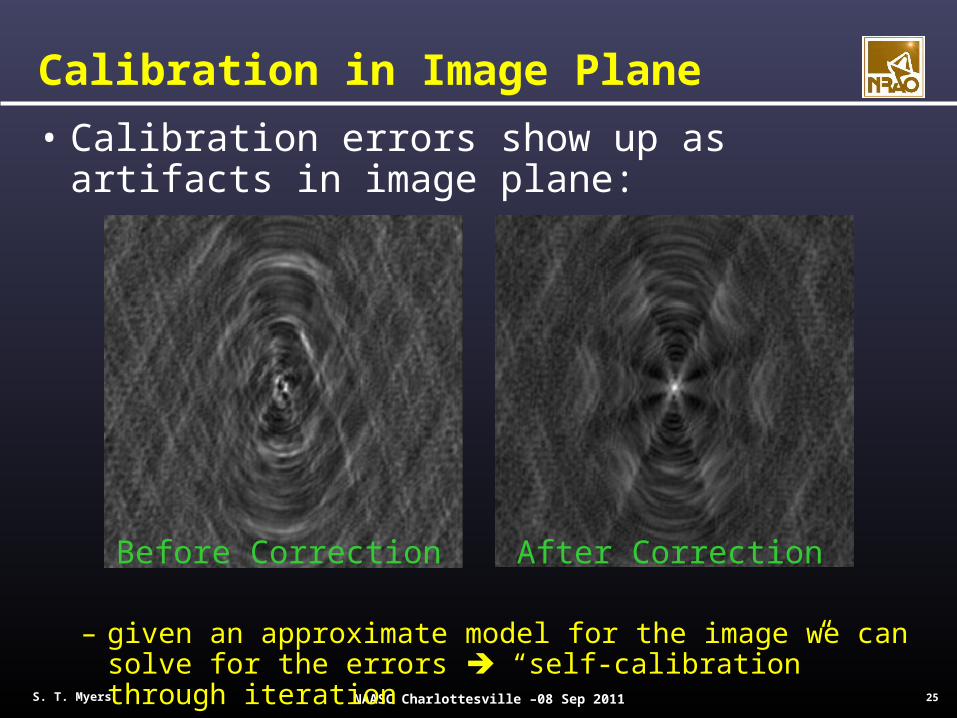
Calibration in Image Plane
• Calibration errors show up as artifacts in image plane:
– given an approximate model for the image we can solve for the errors “self-calibration” through iteration
Before Correction After Correction

26 S. T. Myers NAASC Charlottesville –08 Sep 2011
Pointing Corrections
• Example of direction-dependent errors:– VLA antennas have ~10’’ pointing residual– affects high-dynamic range imaging (>104)– also “squint” between R and L beams
• Work by Sanjay Bhatnagar (NRAO)• Simulation of 1.4GHz EVLA observations• Residual images
– Before correction: Peak 250Jy, RMS 15Jy– After correction: Peak 5Jy, RMS 1Jy
• Can incorporate into standard self-cal• Computational cost ok for now• See EVLA Memos 100 & 84
– Implementing in CASA, testing underway
27 S. T. Myers NAASC Charlottesville –08 Sep 2011
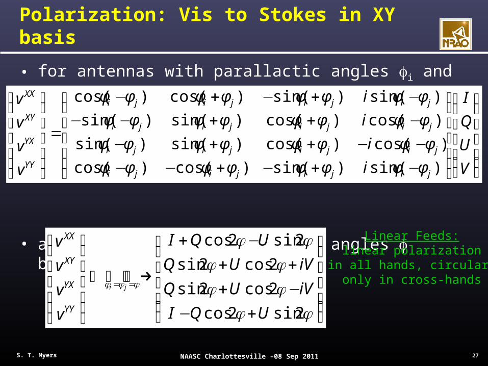
Polarization: Vis to Stokes in XY basis
• for antennas with parallactic angles i and j
• and for identical parallactic angles between antennas:
⎟⎟⎟⎟⎟
⎠
⎞
⎜⎜⎜⎜⎜
⎝
⎛
⎟⎟⎟⎟⎟
⎠
⎞
⎜⎜⎜⎜⎜
⎝
⎛
−+−+−−−−++−−++−−−+−+−
=
⎟⎟⎟⎟⎟
⎠
⎞
⎜⎜⎜⎜⎜
⎝
⎛
V
U
Q
I
i
i
i
i
v
v
v
v
jijijiji
jijijiji
jijijiji
jijijiji
YY
YX
XY
XX
)sin()sin()cos()cos(
)cos()cos()sin()sin(
)cos()cos()sin()sin(
)sin()sin()cos()cos(
φφφφφφφφ
φφφφφφφφ
φφφφφφφφ
φφφφφφφφ
⎟⎟⎟⎟⎟
⎠
⎞
⎜⎜⎜⎜⎜
⎝
⎛
+−−+++
−+
⏐⏐⏐ →⏐
⎟⎟⎟⎟⎟
⎠
⎞
⎜⎜⎜⎜⎜
⎝
⎛
==
φφφφφφ
φφ
φφφ
2sin2cos
2cos2sin
2cos2sin
2sin2cos
UQI
iVUQ
iVUQ
UQI
v
v
v
v
ji
YY
YX
XY
XX Linear Feeds:linear polarization
in all hands, circular only in cross-hands
28 S. T. Myers NAASC Charlottesville –08 Sep 2011
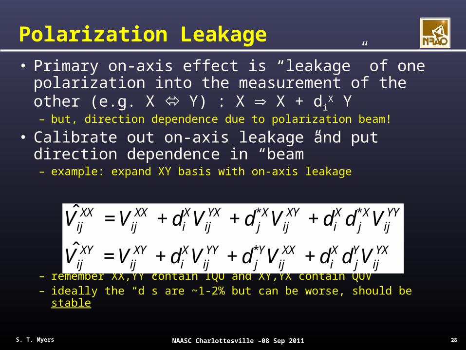
Polarization Leakage
• Primary on-axis effect is “leakage” of one polarization into the measurement of the other (e.g. X Y) : X X + di
X Y – but, direction dependence due to polarization beam!
• Calibrate out on-axis leakage and put direction dependence in “beam”– example: expand XY basis with on-axis leakage
– remember XX,YY contain IQU and XY,YX contain QUV– ideally the “d”s are ~1-2% but can be worse, should be stable
€
ˆ V ijXX = Vij
XX + diXVij
YX + d j*XVij
XY + diX d j
*XVijYY
ˆ V ijXY = Vij
XY + diXVij
YY + d j*YVij
XX + diX d j
YVijYX
29 S. T. Myers NAASC Charlottesville –08 Sep 2011
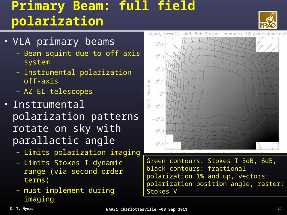
Primary Beam: full field polarization
• VLA primary beams– Beam squint due to off-axis
system– Instrumental polarization off-
axis– AZ-EL telescopes
• Instrumental polarization patterns rotate on sky with parallactic angle– Limits polarization imaging– Limits Stokes I dynamic range
(via second order terms)– must implement during imaging
Green contours: Stokes I 3dB, 6dB, black contours: fractional polarization 1% and up, vectors: polarization position angle, raster: Stokes V
30 S. T. Myers NAASC Charlottesville –08 Sep 2011
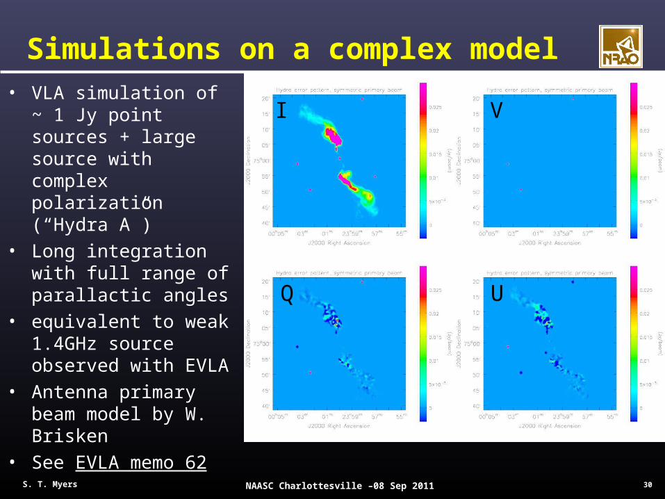
• VLA simulation of ~ 1 Jy point sources + large source with complex polarization (“Hydra A”)
• Long integration with full range of parallactic angles
• equivalent to weak 1.4GHz source observed with EVLA
• Antenna primary beam model by W. Brisken
• See EVLA memo 62
Simulations on a complex model
I
Q
V
U
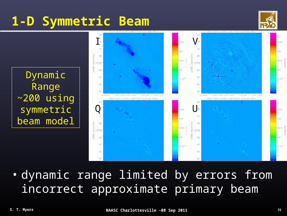
31 S. T. Myers NAASC Charlottesville –08 Sep 2011
1-D Symmetric Beam
• dynamic range limited by errors from incorrect approximate primary beam
I
Q
V
U
Dynamic Range~200 using symmetric
beam model
32 S. T. Myers NAASC Charlottesville –08 Sep 2011
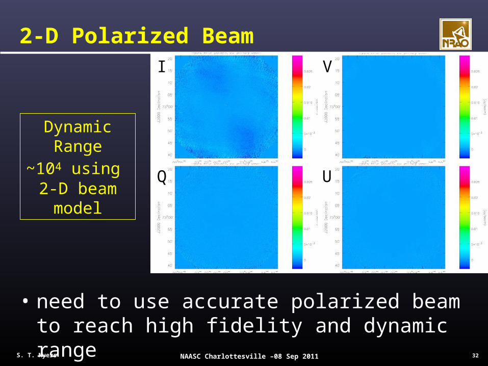
2-D Polarized Beam
• need to use accurate polarized beam to reach high fidelity and dynamic range
I
Q
V
U
Dynamic Range~104 using 2-D beam
model
33 S. T. Myers NAASC Charlottesville –08 Sep 2011
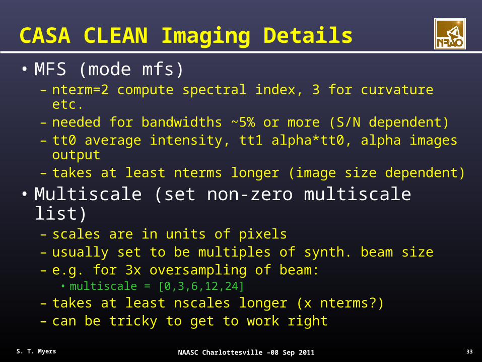
CASA CLEAN Imaging Details
• MFS (mode mfs)– nterm=2 compute spectral index, 3 for curvature etc.– needed for bandwidths ~5% or more (S/N dependent)– tt0 average intensity, tt1 alpha*tt0, alpha images output– takes at least nterms longer (image size dependent)
• Multiscale (set non-zero multiscale list)– scales are in units of pixels– usually set to be multiples of synth. beam size– e.g. for 3x oversampling of beam:
• multiscale = [0,3,6,12,24]
– takes at least nscales longer (x nterms?)– can be tricky to get to work right
34 S. T. Myers NAASC Charlottesville –08 Sep 2011
CASA CLEAN logistics
• clean can be restarted from current state– if imagename used before and files exist and same size– will first recompute residuals from model
• user can input some starting conditions– previous mask (e.g. from previous clean)– previous modelimage
• key toggles– mode: mfs, channel, velocity, frequency– imagermode: ‘’, csclean, mosaic– psfmode: clark, hogbom– gridmode: advanced stuff, eventually a-projection
35 S. T. Myers NAASC Charlottesville –08 Sep 2011
Spectral Cube Considerations
• mode: channel, velocity, frequency– sets the grid of planes in output image cube– will apply doppler corrections on the fly– can set frame info, restfreq, etc.
• data: taken in sky frequency (terrestrial) frame• velocity: include doppler shifts from:
– Earth rotation: few km/s (diurnal)– Earth orbit: 30 km/s (annual)– Earth/Sun motion w.r.t. LSR (e.g. LSRK, LSRD)– maybe galactic rotation to extragalactic frames
• these shifts are time dependent– “Doppler Tracking/Setting” adjust sky freq while observing
– can shift and regrid data before imaging : cvel
36 S. T. Myers NAASC Charlottesville –08 Sep 2011
Continuum Subtraction
• If you have a viable continuum model– e.g. via using mode mfs– can use uvsub to remove from data before imaging– BUT: must have really good accurate model (not likely)
• In practice, subtract “continuum” in data– use task uvcontsub or uvcontsub2
• particularly if strong short-baseline emission
– these fit polynomial to each vis spectrum and subtract• uvcontsub2 can cross spw boundaries
– need to know line-free channel ranges• if uvcontsub need to fit in each spw
– “continuum” not generally imageable• e.g. no closure !!!
37 S. T. Myers NAASC Charlottesville –08 Sep 2011
Odds and Ends
• Oversampling PSF– at least 2.5x, I like 3-4x (whichever rounds well), some
use 5x, no strong impact (but can make imaging longer)
• Boxing– helps guide clean where to pick out real emission,
important when psf sidelobes high/complex and/or when image has complicated structure
– if initial calibration poor, shallow careful clean with boxing will get better model for selfcal (don’t burn in artifacts)
– some cases using csclean (w/cyclefactor) you can “turn it loose”, but be careful before doing this
– we are working on autoclean / autoboxing
38 S. T. Myers NAASC Charlottesville –08 Sep 2011
Flotsam and Jetsam
• What, no clean components?– CASA clean increments the .model image– does not keep track of each iteration component– does not report total cleaned flux until end– does not keep separate multiscale components– might later store cc’s as component lists, but not now– you can mask/edit .model image– you can supply initial “model” using modelimage
• this can come from anywhere! e.g. single dish
• Stopping clean– when you get residual that are noiselike :) or a mess :(– ideally you should get within 2x thermal
• if not, probably calibration errors, bad data, or dyn. range issues
39 S. T. Myers NAASC Charlottesville –08 Sep 2011
Fin
• Final words– the proof of the quality of the data is in the final imaging,
you generally cannot guess this from metrics on the calibrators (particularly when selfcal is possible)
• Anything else?
• Documentation– inline help <task>– online cookbook (massive but in depth)– casaguides