N94-26J179

A Global Approach to Kinematic PathPlanning to Robots with Holonomicand Nonholonomic Constraints

Adam Divelbiss, Sanjeev Seereeram, John T. WenRensselaer Polytechnic Institute

Troy, New York

3

t

PI_I#iP--_II)IN*; PAL_ Ht.ANK NOI FILMffD

https://ntrs.nasa.gov/search.jsp?R=19940021776 2018-08-31T11:48:52+00:00Z

A Global Approach to Kinematic Path Planning toRobots with Holonomic and Nonholonomic

Constraints

Adam Divelbiss Sanjeev Seereerarn John T. Wen

Department of Electrical, Computer and Systems Engineering

Rensselaer Polytechnic Institute

Troy, NY 12180

divelbis@cat.rpi.edu seereeram@ral.rpi.edu wen@ral.rpi.edu

Abstract

Robots in applications may be subject to holonomic or nonholonomic constraints.

Ezamples of holonomic constraints include a manipulator constrained through the con-

tact with the environment, e.g., inserting a part, turning a crank, etc., and multi-

ple manipulators constrained through a common payload. Ezamples of nonholonomic

constraints include no-slip constraints on mobile robot wheels, local normal rotation

constraints for soft finger and rolling contacts in grasping, and conservation of angular

momentum of in-orbit space robots. The above ezamples all involve equality constraints;

m applications, there are usually additional inequality constraints such as robot joint

limits, self collision and environment collision avoidance constraints, steering angleconstraints in mobile robots, etc.

This paper addresses the problem of finding a kinematically feasible path that sat-

isfies a given set of holonomic and nonholonomic constraints, of both equality and

inequality types. The path planning problem is first posed as a finite time nonlin-

ear control problem. This problem is subsequently transformed to a static root findingproblem in an augmented space which can then be iteratively solved. The algorithm has

shoum promising results in planning feasible paths for redundant arms satisfying Carte-

sian path following and goal endpoint specifications, and mobile vehicles with multiple

trailers. In contrast to local approaches, this algorithm is less prone to lrt_ble_r_ suchas sing.ularities and local minima.

1 Introduction

Controlling robot motion, including both manipulators and mobile vehicles, usually

involves the following steps:

1. Kinematic path pla_aning: find a path that satisfies all the geometric specificationssad constraints of a given task.

2. Trajectory generation: index the path with time to generate a dynamic trajectory.

3. Dynamic trajectory following: design a servo controller (possibly incorporating

dynamic information of the overall system) to follow the trajectory.

This paper focuses on the kinematic path planning problem. In contrast to most of

the existing algorithms which are local and reactive in nature, our approach is a globalone which warps an entire path to satisfy all the constraints. A common classification of

constraints involves holonomic versus nonholonomic. If a constraint can be expressed in

terms of the generalized coordinate, it is holonomic; if a constraint involves the gener-

alized velocity and it is not integrable, then the constraint is nonholonomic. Examples

of holonomic constraints include a manipulator constrained through its contact with

the environment, e.g., inserting a part, turning a crank, etc., and multiple manipula-

toes ,c_nst_ t_l_r_ough a common payload. Examples of nonholonomic constraints

'_clttde m_s_ip __s _ mobile vehicle wheels, local normal rotation constraints

_ft fnger contacts in _ and conservation of angular momentum of space

robots. There may be other design amstraints imposed by the task, for example,

equality constr_nts snch as the desired termin_ configuration, specified end effectorpath, etc., and inequality constraints such as manipulator joint limits, self collision andenvironment collision avoidance constraints.

There is abundant literature on path planning for redundant robots, which are

examples of systems with holonomic constraints, and mobile robots which are examples

of systems with nonholonomic constraints, but seldom on both. The principal reason

is that in the local approach, the two problems are fundamentally different in that

redundant robots can in general move in all directions locally in the configuration

space, but nonholonomic systems can only move in certain directions. Consequently,

the issues related to redundant robots are singularity, redundancy resolution, joint

cyclicity for cyclic end effector paths, etc., and, for nonholonomic systems, the main

issue is in finding a path whose tangent lies within the admissible directions. There

are also commonalities in the two classes of problems:

1. Kinematic models are linear in control (i.e., admissible velocities).

2. Collision avoidance and joint limits are represented as a set of inequality con-straints.

In our approach, the entire path is iterated toward a solution. Therefore, in this

framework, whether the constraint is holonomic or nonholonomic does not make a

fundamental difference; a more important distinction is between equality and inequality

constraints. Indeed, path planning for redundant robots and mobile robots are treated

in exactly the same way in our uroposed approach.

The manipulator path planning problem is traditionally based on geometric ap-

proaches. (Comprehensive surveys can be found in [1, 2, 3].) The majority of these

use the configuration representation of the manipulator and the obstacles and joint

limits (as originally proposed in [4]). In this formulation, the path planning problem

is reduced to finding a feasible path for a single point. Various tools from geometry,

topology and algebra have been utilized to develop methods such as roadmap, cell

decomposition, and potential field methods. The drawback of the configuration space

approach is that the configuration space can become high dimensional for manipu-

lators with several joints and mapping out the free region for a redundant arm in a

cluttered environment is a time consuming process and produces large graphs to be

searched. Recently, some work has emerged which focuses on minimizing this growth

in computation by incorporating heuristics [5, fl].

The specific issue of redundancy resolution in redundant manipulators has tradi-

tionally been addressed by using the Jacobian pseudo-inverse [7, 8, 9, 10], which is

a local, or point-wise on the path, approach. This approach is simple to use, has

low computational overhead, and can be combined with the local potential field forcollision avoidance. The drawbacks include local minima, breakdown near or at sin-

gularities, and non-cyclic or even unstable joint motion for cyclic end effector paths[11, 12, 13, 14]. Some global techniques based on optimization have also been proposed

[15, 16, 17, 18, 19], but the resulting two-point boundary value problem (TPBVP) isdifficult to solve for complex problems.

In the rapidly accumulating literature on nonholonomic motion planning, there

appears to be a similar dichotomy of approaches: graph search based methods as

in [20, 21, 22, 23, 24, 25, 26] and analytic methods [27, 28, 29, 30, 31, 32, 33, 34,

35]. The former class tends to be computationally inefficient but can handle generalconstraints, the latter class gives elegant insights into the structure of the solution but

may generate impractical paths. Recently, some important insights have been gained

by linearizing the kinematics equation about a non-stationary trajectory instead of

a fixed equilibrium. It is shown in [36] that the linearized time varying system is

frequently controllable, and a locally stable feedback controller can be designed. In

[37], a globally stable feedback controller is also found. Based on this approach, a

general procedure for designing globally stable time varying feedback controller hasbeen obtained [38].

A common starting point for the analytic approaches to the path planning problem

is to pose it as a general nonlinear control problem. Using this framework, we present

a new method of solving the path planning problem in this paper. The formulation is

based on converting the nonlinear control problem into a nonlinear algebraic equation.

The problem then becomes a nonlinear root finding problem in which the dimension

of the search space is very high (infinite if {u(t) : t E [0, 1]} is taken from an infinite

dimensional functional space) compared to the number of equality constraints (for

the end point constraint). The nonlinear root finding problem is further converted to

an initial value problem (IVP) which is much easier to solve than the usual TPBVP

typically arising in the optimization approach. Under some additional assumptions,

the IVP can be shown to be wellposed [39] and a variable step size ODE solver is used

to propagate the solution. Examples ranging from a front-wheel driven car to triple

trailers to nine degree-of-freedom (DOF) manipulators have been successfully tackled

[40, 41, 42]. A similar approach has also been proposed independently in [43, 44]

for kinematic path planning with only the end point constraint. For this case, the

wellposedness property of the IVP is shown to be generic.

Since the dimension of the search space is very high, there are many possible solu-

tions to the root finding problem which results from the path pla_aning problem. For

any practical applications, additional constraints must be placed. We have adopted an

approach similar to the global exterior penalty function method [45, 46] which convertsinequality constraints into a zero §ndlng problem. This differs from the familiar arti-

ficial potential field method which is an interior penalty function (or barrier function)method in that the initial guess may be infeasible.

The inequality constrained case can then be combined with the equality constraints

into an augmented zero finding problem. Non-configuration space constraints, for

example, constraints involving corners of a vehicle, body of the robot, etc., can also be

incorporated in this formulation.

The global path planning approach that we have proposed has been applied toexamples involving redundant manipulators and nonholonomic vehicles. We note the

following attractive features of this algorithm:

1. Both equality and inequality constraints can be included in this formulation.

The constraints can be nonlinear in the configuration variable, so task space

constraints (which involve nonlinear kinematic function of the configuration vari-ables) are also allowed.

2. The initial guess does not have to be feasible. The planner iteratively warps thepath until all constraints are satisfied.

3. This approach emphasizes feasibility over optimality in contrast to other globalapproaches. Once a feasible solution is found, optimality can be incorporated as

a secondary constraint.

4. The IVP formulation is computationally easier to solve than the TPBVP.

5. There are additional points related specitically to redundant manipulators:

• Goal task variability: This approach can be used for finding a feasible joint

sequence from a fixed initial configuration to a specified Cartesian or jointspace goal - the path planning problem - as well as for global redundancy

resolution along a specified Cartesian path.

• Singularity robustness: The global nature of the planner avoids the Jaco-

bian singularity problem inherent in local methods. While the controllabil-

ity about a configuration is lost at the singularity, the algorithm can proceed

as long as controllability about the planned path, which is a much looser

condition to satisfy, is retained.

• Incorporation of additional equality constraints: As an application of this

capability, the planner can generate cyclic joint space motion for a specified

cyclic task space motion.

There are also additional points related specifically to nonholonomic systems:

• The planner only requires local controllability about a path in every iteration

but does not require controllability about a configuration. This is importantsince the latter is not satisfied for nonholonomic systems.

The rest of this paper is organized as follows: Section 2 describes the theory be-

hind the proposed algorithm. Section 3 describes the global exterior penalty function

method to handle inequality constraints. Section 4 shows a number of simulation ex-

anaples involving path planning for redundant manipulators and mobile vehicles withtrailers.

2 Kinematic Path Planning Subject to Equal-

ity Constraints

In this paper, we consider the problem of finding a continuous path that links the

specified initial and final configurations while satisfying a set of specified equality and

7

inequalityconstraints (which may be either holonomic or nonholonomic). To state this

problem precisely, we first represent a kinematic model as a control system:

4(_)= _(t) ; q(O)= qo (1)

where q E R '_ is the configuration variable and u E R n is a pseudo-velocity consid-

ered as the control input. Note that since this is a path planning problem, the path

variable, t, is arbitrarily normalized to be within the interval [0, 1]. There may also

be additional holonomic and nonholonomic constraints imposed along the path. If the

constraints along the path are directly incorporated in the kinematics equation, these

constraints are treated as hard constraints. If the planner iteratively updates the path

until the constraints are within a certain tolerance, these constraints are considered as

soft constraints. We first state the general path planning problem with soft constraints:

Define u = {u(t) : t 6 [0,1]} and q = {q(t) : t 6 [0,1]}. Given (1),

find u_ e L:([0,1];R n) such that q(t) satisfies (1)and c__(q,u) = 0 wherec. : L2([0, 1]; IU_) x L2([0, 1]; R n) --* Y is a given equality constraint function

for a specified normed linear space, Y.

The constraint function _cmay include physical constraints, such as nonintegrable ve-

locity constraints on wheels (nonholonomic) and contact constraints of manipulators

(holonomic), or artificial constraint such as the desired end effector path of a redundant

manipulator. Pathwise holonomic constraints can be represented as

_(q,__)(t)= kl(t,q(t)) ,t e [0,1] (2)

and pathwise nonholonomic constraints are of the form

-_(t, _)(t) = k2(t, q(t), 4(t)) , t e [0, 1] (3)

and can not be integrated to a constraint only involving the configuration variable.

In many applications, k2 is linear in 4 and invariant in t, i.e., k2(t,q(t),(l(t)) =

K2(q(t))(t(t). A system may also be subject to what is known as second order nonholo-

nomic constraints (for example, for a manipulator with unactuated joints [47]).

For the path planning problem with hard constraints, the path constraints in (2)

and (3) are explicitly removed. In the holonomic case, write (2) in the differential form:

okl(t, q) + ok,(t, q)_ = o. (4)Ot Oq

Denote the Jacobian matrix _ by J(t, q). If J is a fat matrix (as in the caseof redundant manipulators) and is nonsingular, then the constraint can be explicitly

incorporated in the kinematics, resulting in

__0k_(t,q)= -s+(t,gj _ + Y(t,q)_ (5)

where J+(t, q) denotes the Moore-Penrose pseudo-inverse of J(t, q), ](t, q) is an arbi-

trary full rank matrix whose range coincides with the null space of J(t, q), and _ is thenew effective control variable.

In the nonholonomic case, if the constraint is linear in u, then the constraint can

be eliminated, resulting in a new kinematic equation:

4 =K2(q) (6)

where v E R "_ is the new effective control variable (m is the dimension of the null

space of K2(q), assuming it is a constant).

The general planning problem can now be restated as before except the kinematic

equation is modified as below to incorporate the path constraints:

_t) = h(t,q(t))÷ f(t,q(t))t_(t) ; q(O) = qo. (7)

The drift term, h(t, q), is zero in the case of nonholonomic constraints linear in _. The

equality constraint function may involve only the end configuration:

= qfl) - qd (s)

where qd is the desired final configuration. In the case of redundant manipulators, joint

cyclicity implies qd = q0.

For the path planning problem as formulated above with either soft or hard con-

straints, our approach is based on converting the differential description of the problem

into an algebraic form. First consider the soft constraint formulation. Recall this case

involves a very simple kinematic equation given by (1). For a given initial configuration

q0, _q can be related to u via a linear causal map, D_, and an initial condition vector,

fo:q = D_u_._- q._. (9)

Define the constraint error as

z = + (10)

The path planning problem is now reformulated as a nonlinear root finding problem

for c as a function of u_ Nonlinear root finding has the reputation being numerically

challenging [48, §9.6]. However, the situation here is different than the general casein that the dimension of the search variable, u_, is typically much larger than the

dimension of the constraint eo lation. Consequently, there are a very large number

of roots and finding one of these roots is less difficult than the general root finding

problem. However, equality constraints alone may not produce physically realizable

solution; we shall see how this formulation can be extended to inequality constraints

in the next section.

To find a u_ that solves y --0, our basic strategy is to lift a path in Y that connects

an initial guess y(0) to zeroto a path in L2([0, 1]; Rrn). Then the end point of the path

in L2([0, 1];R m) is a solution that satisfies the stated equality constraint c(q,u_) - 0.

To achieve this, we set up the path iteration equation:

dy d_ (11)d'r - G dr

where

G = Vqfi D__+

9

If G is full rank, or, equivalently, the null space of G* (the adjoint map of G) is zero,

then any one of the following algorithms can be applied to update u_u_:

d_ G+ d_ _ (12)

where G + is the Moore-Penrose pseudo-inverse of G, and Y--dis any desired convergence

profile of y_ in "r and y_d(0) = y_(0), for example, we can choose y_d(r) = e-_'y(0),for exponential convergence. However, this rate may not correspond to the physical

convergence rate since (12) may take much longer to solve. In practice, Eq. (12) maybe solved by an ODE solver or discretized with the time step in-r found by line search.

In the hard constraint formulation and with only the end configuration constraint

(i.e., c_(q,u) = q(1) - qd), the equality constraint error can be written as

y_= F(u) - qd (13)

where F maps the control, u, (for a given q0) to the final configuration. The analytic

form of F is in general difficult to find, and will not be explicitly required. The system

(7) is globally controllable if and only if the nonlinear map F is onto, and the system

is locally controllable around u. if and only if V__F(u.) is a linear onto map. Localcontrollability around u is equivalent to the controllability of the linear time varying

system obtained after linearizing (7) around _qand u.. The path planning problem can

be iteratively solved as before using (12) but with

G = V__F(u_).

A sufficient condition for convergence is that G is full rank for all r, or, equivalently,

the time varying linearized system with u_(v) is controllable. For systems without drift,

such as nonholonomic systems, it has been shown in [43] that this condition is generic.

Equation (12) can be solved by an ordinary differential equation (ODE) solver with

an initial guess of u(0) such that the full rank condition is satisfied. In addition, y__a('r)

can be used to check the accuracy of the solution, y_(v), at each 7-. It can be shown

that if u_(0) is sufficiently close to a solution, then the wellposedness of the IVP (and

its convergence) is assured. As stated before, the wellposedness of the IVP in thehard nonholonomic constraint case has been shown to be generic and there has been

a surge of recent interest of this technical issue [39]. For the general problem, the

wellposedness condition remains an important research topic. In all of our simulation

experience involving equality constraints, this has never been a problem. In the next

section, when constraints are included through the global exterior penalty function,

the issue of weUposedness becomes more severe.

An interesting aspect of this approach is that in (12), ([ does not affect the guaran-

teed convergence rate (specified by a), though it does affect the way _ converges. Since

the dimension of _ is much larger than _, there is much freedom in _ to affect the even-tual convergent solution. For example, _ may be chosen so that additional constraints

in _ may be satisfied. We have explored choosing _ via quadratic programming with

some success, but more research needs to be done in exploiting this degree of freedom.

There are other possible choices of 2, for example, in the soft constraint case,

d_ G" d_= (14)

i0

du_ G'y_ dwd 1

dv IG_.y[[

The trade-offs between computational load and convergence speeds between theseschemes axe yet to be fully explored.

The initial guess _u(0) will clearly affect the convergence. We have not extensivelyexplored an intelligent procedure (perhaps based on past experience) for this selection.

In all of our examples, the initial conditions are simply chosen to avoid the rankdeficiency of G.

In the algorithm described above, it is critical to be able to calculate G efficiently.

Since G relates an infinitesimal variation 6u_ to a corresponding infinitesimal variation

6c_, it can be computed based on the linearized kinematic equation (and the constraint

equation in the soft constraint case). This procedure is described in detail in [49], andhas been used in all of our examples.

3 Kinematic Path Planning Subject to Inequal-

ity Constraints

in the previous section, only equality constraints are considered. However, for realistic

problems, there are also many inequality constraints which need to be enforced. For

problems involving equality constraints only, the obtained path is frequently undesir-

able. For example, in the case of a tractor with twin-trailers, the front wheel angles ofthe tractor may go through an unrealistically large range motion, the trailers can be-

come jack-knifed, and the entire vehicle may go through several complete revolutions;

in the redundant arm case, the joints can violate joint limits, and there may be self

collision or collision with other objects in the workspace. Clearly, if this algorithm is

to be used in practical applications, additional constraints must be incorporated. In

this section, we present an approach similar to the exterior penalty function method of

[45] and which has so far been shown to be very effective in addressing the inequalityconstraint issue.

There are three basic approaches to address the inequality constraints:

• Convert the inequality constraints into equality constraints by defining a functionthat is zero when the constraint is satisfied and non-zero when the constraint is not

satisfied. Once this is done, the zero finding approach of the previous section can be

applied to find a zero solution which corresponds to a feasible path.

• If the feasible region is convex polyhedral, then linear programming or quadratic

programming can be used to select the free variable _ in (12) without affecting the

convergence of the equality constraints.

• Pre-waxp the vector with a multiplicative potential function _b(q) which is zero on

the boundary of the inequality constraint and positive inside the feasible region. It has

recently been pointed out in [44] that as long as the initial path _q(0) lies strictly within

the feasible region, then the same algorithm (12) can be applied to iteratively move yto zero.

We have extensive experience with _the first two approaches. The first approach has

proven to be very effective, though there are currently no (genericity) results on the

11

full rank gradient condition as in the equality constraint case. The second approach is

computationally intensive due to the need to repeatedly solve a constrained optimiza-

tion problem. It is perhaps best used as a local optimization refinement in conjunction

with the first approach. The third approach has just recently been suggested and is

computationally untried; we intend to pursue this direction in the proposed research.

For the remainder of this section, we will elaborate on the exterior penalty function

approach.

Suppose the feasible region is defined by a set of p inequalities:

gl(_,_) _ 0 (16)

where gl is nonlinear and assumed to be as smooth as needed, and <_ is interpreted

as a component-wise relationship. These constraints may be directly placed on the

configuration variables such as joint limits or on other variables such as the end effector

of a manipulator, vehicle boundaries, etc. Without loss of generality, we shall consider

the hard constraint case for the discussion below. Let the relationship between _ and _

be denoted by q = F_.(__). By substituting this relationship, the constraint inequalitiesare transformed to

g(F(__),__) < 0 (17)

or more simply expressed as

g(u) < O. (18)

Suppose now we wish to constrain the states of the system to stay within the feasible

region defined by the task space. We then define a penalty function corresponding to

the i th system state as:

N { .. A= "r.gA") > 0 (zg)j=l 0 < 0

where )_ > 1, gji's correspond to the constraint applied to state i at discrete time j and

"yyi's are constant weights. This function is nonzero when state i violates the constraints

at any time along the path, and is identically zero only when all constraints are satisfied.

For this penalty function, the penalty imposed depends upon the constraint violation

raised to the Jkpower. Therefore, the penalty function approaches infinity as the system

makes ever increasing incursion out of the feasible region. Of course many other choices

for the constraint function are also possible. For example, another penalty function

which we use frequently is the following:

N{.i=1 0

gi,(") > 0(20)

< 0

where r, > i and _ > 0. This penalty function is bounded by the sum of the "yji's, and

is therefore in some sense less harsh than the previous penalty function. In practice

we have seen that the second penalty function gives faster convergence than the first,

in cases where the vehicle makes large excursions outside of the feasible region. This

advantage in convergence stems from the fact that X7_zi(_) is smaller for the second

constraint function than for the first when large constraint violations occur, causing

12

the IVP to be more wellposed for the second constraint function. For either penalty

[function, the composite constraint vector is defined as z = zl ... z,_

We now have a situation similar to the unconstrained case: Find u so that y = 0

and z = O. The same approaches described in Section 2 can now be applied. Using thehard constraint formulation, the new differential equation in u_.now becomes:

where,

- = +zd (21)

Gl(u-) a [ G ]= V_z(u) (22)

and Y--aand Zd describe the desired path in r that links the initial error to zero. Thegradient of z(u) can be easily obtained via chain rule and the linearized kinematic

equation [49]. The convergence of this algorithm now requires the full rank condition

on G1 in each iteration. Note that in (21), there is again a free parameter _(r). The

extra degrees of freedom offered by _(v) may be used to satisfy additional optimalityconsiderations.

The penalty function formulation we have presented allows for a wide range of

constraint types. Up to this point we have considered constraints which apply directlyto the configuration variable of the system, but the formulation allows constraints to

be applied to non-configuration variables as well. In any practical application it is

not enough just to constrain the origin of the system inside a feasible region. The

boundaries of the system must stay inside as well. For instance, for a single planar

body, we relate any point p on the boundary to the configuration variable q by thenonlinear transformation:

Py q2 sin(q4) COS(q4) ry

where r_ and r_ are the x and y positions of the boundary point in the body frame.

The same penalty function which applied to q before now applies to p, gj(p(qj(u_))).

A similar transformation can be obtained to relate boundary points of multi-bodiedsystems to the configuration v::riable.

The penalty function formulation also allows for a wide range of feasible region

types. For instance, when the feasible region is polyhedral, g takes on particularly

simple form:

g(_) = A_- b.

We have looked at this type of constraint extensively. In fact, this constraint type is

always used when limiting wheel or jackknife angles on wheeled vehicles. This type of

constraint is simple to use but the feasible region is necessarily convex:

The penalty function can be used to enforce both convex and non-convex, non-

polyhedral constraints. For instance, supposed it is desired to drive the system while

keeping boundary points outside of an circular region. The constraint g at each time

j can then be expressed as:

gj(p) = - =0)2- - 2 + r2

13

where z0 and Y0 are constants, r is the radius, and p is a boundary point as described in

(23). We have had much success in using this formulation with cars and tractor-trailer

vehicles and present an example in the next section.

In the preceding discussion, system constraints are expressed as analytic functions

of the configuration variable. "But again, in practical situations it may not be possible

to adequately represent the constraints by analytic functions. In particular, for highly

unstructured environments it may require great effort to find an appropriate analytic

function, and once found, it may be computationally intensive to apply it. Therefore,

we propose a method based upon the contour map built up from the task space obstacle

boundaries. First, suppose that the feasible region is defined by a set of p inequalitiesof the form:

g2(F(_u)) < 0 (24)

where g2 is nonlinear, smooth as needed, and < is component-wise. The gradient of

g2 with respect to u_ is then obtained by applying the chain rule,

V_J2 = [V_F]TvqJ2. (25)

Note that in this equation, V,,=_F is independent of the constraints and that Vq_g2

depends solely upon the constraints. Therefore, rather than compute g2 and Vq_g2explicitly using analytic functions, it is possible to use a lookup table to compute these

values. For g2, the lookup table contains the cost for each point in a grid covering the

task space. For V_.g2 the table contains the gradient components for each point on thegrid. As before, this formulation will also work for non-configuration variables. Sincethe exterior penalty function approach is used, the contour map is zero everywhere

inside the feasible region and non-zero outside. We have just begun using this method

for path planning and have so far had good success. An example of the contour map

method applied to a car is given in the next section.

In this, and the previous sections, we have used the notation u_.to denote the set

of control inputs applied to the system at each point in time along the path. Forthe continuous case this set contains an infinite number of elements. Therefore u in

vector form would be an infinite dimensional vector. However, in order to implement

the algorithm on a digital computer u_ needs to have finite length. The first obvious

step would be to discretize u(t) using the standard basis. We have used this approachextensively and have obtained good results from it. Another approach we have tried is

to use the first N elements of the Fourier basis to approximate u(t). In this formulation,

for each discrete time j we represent the control input as:

uj = @(jAt)_ (26)

where _ is a matrix containing the Fourier basis elements and _ is the constant vector

of Fourier coefficients. In this formulation, X uniquely describes the control over all

time, since it is independent of time. Now for a given initial configuration _, q can berelated to _ by a causal map, FI:

l = (27)

Furthermore, substituting F1 for F and _ for g in all previous equations, we see

that all previous methods still work. The full advantages and disadvantages in using

the Fourier basis formulation rather than the discrete basis is unknown at present.However, in the case of driving a car around a circle, we have observed that the discrete

basis formulation has great difficulty arriving at a solution whereas the Fourier basis

formulation solves the problem with relative ease.

4 Examples

We have appliedthe algorithmto a largenumber of computer simulationexamples

and experimentallyto a mobile robot. For illustrationpurposes,we includeseveral

examples involvingthreedifferentwheeledvehiclesand a point-to-pointpath planning

of a 4R planararm and a 9DOF arm likethe one in our lab (seenext sectionon a

fullerdescriptionofthisarm).

In thefirstexample,we considerthe parallelparkingofa doubletractor-trailer.A

truedouble tractor-trailer,likethoseseen drivingon the highways,actuallyconsists

of a tractorwith threetrailers:two longtrailersconnectedby a comparativelyshort

trailer.The shorttrailer,or dolly,makes any backing-up situationextremelydifficult

in that smallbackward motions can produce largejackknifeanglesbetween the dolly

and the trailers.In fact,itisknown thatwith a human operatorone must,in general,

disconnectthe end trailerand dollybeforeany backward motions are attempted.

In the example below,shown in Fig.1-2 below,the frontwheelsare constrained

to :t:35° and the jackknife angles (the jackknife angle is defined as the angle between

the center line of one trailer and the center line of an adjacent traihr) are constrained

to +50 ° . The limits on the jackknife angles are sufficient to ensure that none of

the trailers collide. In this example the algorithm required about four hundred fifty

evaluations of the right hand side of the differential equation to achieve a tolerance on

the potential fields of 0.01. The penalty function method used here is simply the first

convex, polyhedral method mentioned in the previous section.

-$ o 5

s-t_m

Figure 1: Parallel Parking Path of a Double Tractor-Trailer with Constraints

The next example is presented to demonstrate the versatility of the algorithm with

regard to the type of constraint applied. In this example, it is desired to drive atractor-trailer vehicle around a circular obstacle while remaining within a rectangular

region limiting motion along the z-axis. To further complicate the example, two other

15

I

oJ

0.6

0.4

i o_02

_0.,,I

..O.t

41.|

0 0,_ 0.4 _t om o.2 _4 oA &| I

Figure 2: Parallel Parking Path of a Double Tractor-Trailer with Constraints

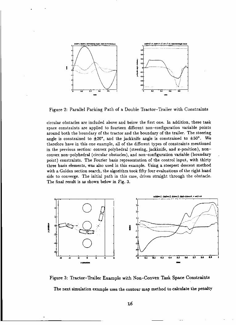
circular obstacles are included above and below the first one. In addition, these task

space constraints are applied to fourteen different non-configuration variable pointsaround both the boundary of the tractor and the boundary of the trailer. The steering

angle is constrained to 4-20 ° , and the jackknife angle is constrained to 4-50 ° . We

therefore have in this one example, all of the different types of constraints mentioned

in the previous section: convex polyhedral (steering, jackknife, and =-position), non-

convex non-polyhedral (circular obstacles), and non-configuration variable (boundary

point) constraints. The Fourier basis representation of the control input, with thirtythree basis elements, was also used in this example. Using a steepest descent method

with a Golden section search, the algorithm took fifty four evaluations of the right hand

side to converge. The initial path in this case, drives straight through the obstacle.

The final result is as shown below in Fig. 3.

t

:iI o

-6 -4 -2 O 2 4

:-Fe,_on

s_d_ I, dmhmt2, dcc=:c.t, dmh-de_x4, + ,etS.x4

4

......j::%:ii!01 .7"-_: " *"_**_'***'_._s" *. * / ..°*"

-I

-2

4

"So o'., o_ 0.3 o., o_ 0.6 _7 i, o'.,time

Figure 3: Tractor-Trailer Example with Non-Convex Task Space Constraints

The next simulation example uses the contour map method to calculate the penalty

I6

function. In thisexample,it is desiredto drivea cararoundacircularobstaclewhileremaininginsideof a circularregion.Sevenpointsaroundtheboundaryof thecarareusedfor non-configurationvariableconstraints.Thefront wheelsareconstrainedto=k15°. TheFourierbasiswasonceagain used to represent the control input along the

path. This example took about one hundred evaluations of the right hand side using

a discretized version of (21) with Golden section search to find the optimal step size.

The initial path drives straight through the obstacle. Below, the first set of plots, in

Fig. 4, show the car and path in the context of the task space. The second set of plots,

in Fig. 5 show the contour map used in this example.

i_k

solk_xl,dashZx2odO_ux3,dag_-dmsx4

2

i i

0

1

-2

-3

% 0._ 0.2 0.3 0'., o; 0:6 0:7 o'.s 0'.9

time

Figure 4: Path Planning with Contour Map Method

Figure 5: Plots of Exterior Penalty Function and Contour Map

In the final wheeled vehicle example, we present experimental results of applying the

17

pathplanningalgorithmto anactualmobilerobot.Therobotis actuallyaonequarterscalemodelcar,completewith apassivesuspensionsystem,on-boardIBM compatible48633-MHzcomputer,andwheelencodersfor usein dead-reckoningfeedback.Thedesiredpathwasa simpleparallelparkingpathwith constraintsonly on the steeringangleof ±15° whichis the physicallimit of the car. The purpose of this experimentwas to determine if a real robot can actually follow a path generated by the planning

algorithm. In this example, the path was generated, and then a velocity profile was

imposed. A simple, Lyapunov function based, feedback controller was used to try and

track the path. Although there is some error in tracking the path, it is obvious from

the plots below, in Fig. 6-7 that the path is such that the real car can follow it. The

tracking errors are due in part to error in the dead-reckoning feedback and to thecontroller used.

!

6O

4C

2C

0

-20

..6O

solidmacvzaL dolk-nla,dezi_'cL units in inches

-20 0 20 4O 60 8O i00

z-posit_

Figure 6: Parallel Parking of Catmobile: Experimental vs. Simulation Path

Various examples of redundant manipulators are presented which incorporate both

joint and task space inequality constraints. Key features of this approach include vari-

ous possible goal task specifications (from end-point only to entire path specification),

joint path cyclicity, and robustness to manipulator singularities. Inequality constraintsare handled by the global penalty functions and a linear inequality set description as

shown in Sections 3. Simulations were performed using Matlab with computationallyintensive routines coded as Matlab-callable C routines (cmex files). Note that the end

effector constraint is treated as a soft constraint here as compared to the nonholonomic

constraint considered above which is treated as a hard constraint.

The first example illustrates the joint sequence for a 3R planar arm required to trace

out the tip path shown while remaining within a set of task space boundaries (Fig. 8).

The path shown in Fig. 8 includes an intermediate joint vector in which links 2 and 3

become aligned - equivalent to a pose switch for spatial arms. Local planning methods

typically encounter difficulty in handling pose changes since they correspond to arm

singularities, and the arm Jacobian losing rank. The present algorithm executes the

pose switch smoothly, while tracking the desired tip path. In the next situation (Fig. 9)

a 4R arm is required to traverse to specified coordinates X I. The obstacles are chosen

18

|1

W

6o

4O

20

0

o_

..400 ,o 2o _o _o _o _o 7o

tl (second)

s_. dlx=desired, solid_cmsl; or:dssh d_x=desimd.0.3

i!

m

-o.i

-o._

-0.4

",..i J, , "=;",,o 2o _o _ s'o _ _o

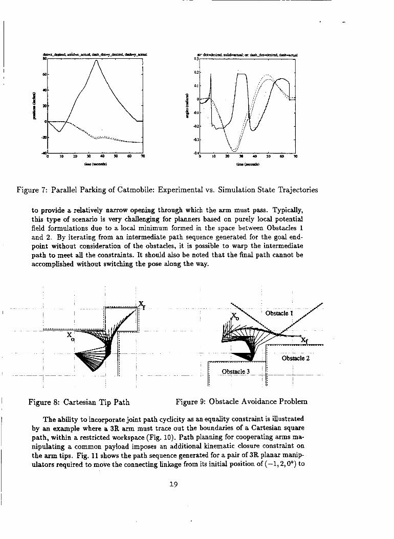
Figure 7: Parallel Parking of Catmobile: Experimental vs. Simulation State Trajectories

to provide a relatively narrow opening through which the arm must pass. Typically,

this type of scenario is very challenging for planners based on purely local potential

field formulations due to a local minimum formed in the space between Obstacles 1

and 2. By iterating from an intermediate path sequence generated for the goal end-

point without consideration of the obstacles, it is possible to warp the intermediate

path to meet all the constraints. It should also be noted that the final path cannot be

accomplished without switching the pose along the way.

' i........................................_ ..................i.........................................i...__Z !.............ob&ie2............

Figure 8: Cartesian Tip Path Figure 9: Obstacle Avoidance Problem

The ability to incorporate joint path cyclicity as an equality constraint is illustrated

by an example where a 3R arm must trace out the boundaries of a Cartesian square

path, within a restricted workspace (Fig. 10). Path planning for cooperating arms ma-

nipulating a common payload imposes an additional kinematic closure constraint on

the arm tips. Fig. 11 shows the path sequence generated for a pair of 3R planar manip-

ulators required to move the connecting linkage from its initial position of (-1, 2, 0 °) to

19

agoalpositionof (2,2,45°).In theplanarexamplesshown,theapparentcollisionsofthe links with the obstacle boundaries arise out of the fact that checking is performed

for the tips of each link only. A more complete collision detection procedure is being

developed for spatial arm planning.

: I

H i............... . ......................... I ...................

I

: ................. f ..................

X o, Xf ,,

I

: ',

.................... i ................. i ......

: . I •

• . II :

":_:.):: : : .: ".. '. ::., .. ... :..:..

T

Figure 10: 3R Cyclic Path Figure 11: Cooperating Arm Problem

The remaining examples illustrate applications to a spatial redundant 9 DOF arm.

This consists of a PUMA 600 manipulator mounted on a platform providing additional

linear, rotate and tilt joints. (See [50] for details of the CIRSSE dual-arm robotic

testbed.) Fig. 12 shows the output sequence for joint path end-point planning to a

specified task space position/orientation in the presence of an obstacle. Fig. 13 shows

the path sequence generated for a path following task incorporating a straight line

translation coupled with a rotation of 180 ° about the tip Y axis. Because of the

manipulator joint limits, this can only be accomplished by switching the PUMA's pose

from elbotg-up to elbo_g-dourn at some intermediate point. As in the planar examples, the

present algorithm accomplishes a smooth transition between these arm configurations.

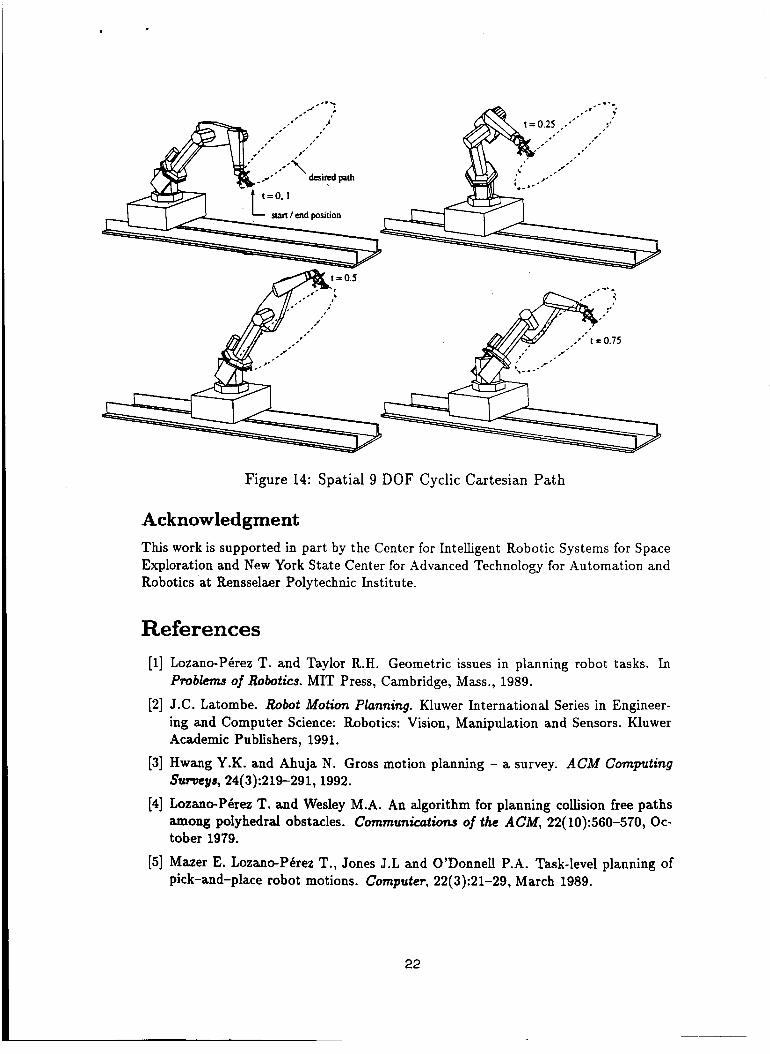
The final example (Fig. 14) illustrates a cyclic joint path sequence computed for the

arm to follow a circular task space path while maintaining a fixed tool orientation

(perpendicular to the plane of the circle).

For the cases shown, the planar examples required from seven to ten iterations to

reduce the task error and meet all the constraints, while the spatial examples ranged

from ten to twenty-five iterations. Discretization levels ranged from R" -- 10 to 40

in size. For the 9 DOF redundant arm planning scenario, this represents a small

computational load for the Sun SPAttC-station used. workstations. For problems of

larger size, this technique can be applied recursively to the desired discretization level,

thereby keeping the individual iteration array operations small. The ability to apply

the algorithm to the global problem (even at the coarsest resolution) is essential for

2O

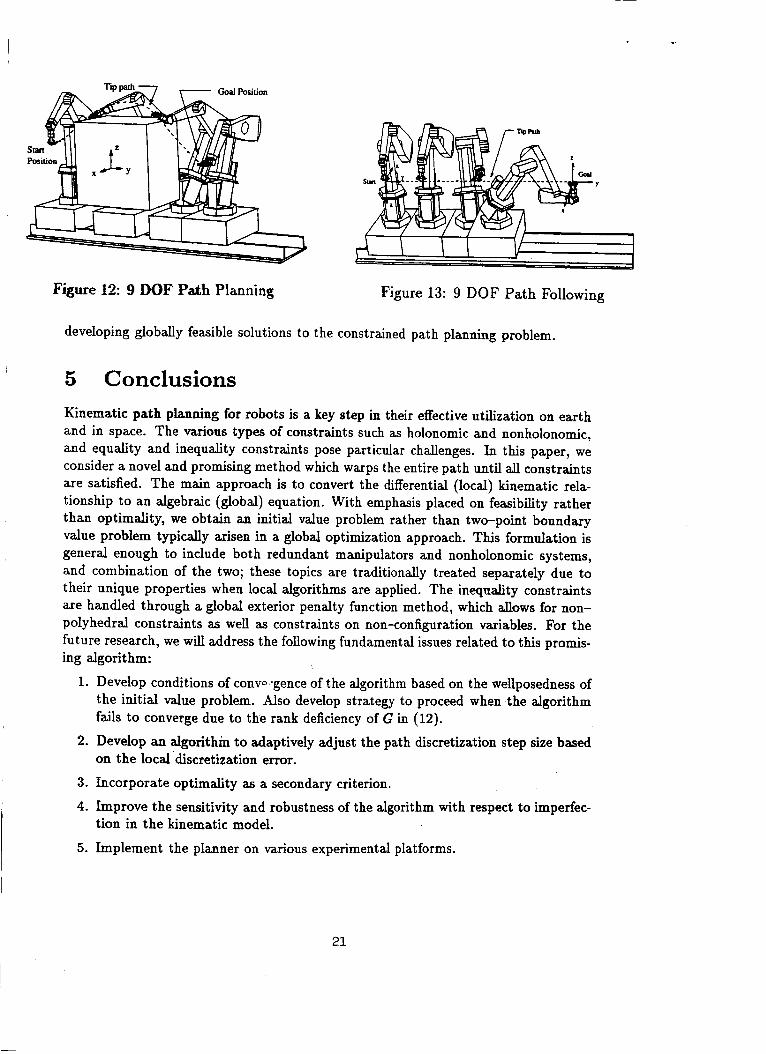
Figure 12:9 DOF Path Planning Figure 13:9 DOF Path Following

developing globally feasible solutions to the constrained path planning problem.

5 Conclusions

Kinematic path planning for robots is a key step in their effective utilization on earth

and in space. The various types of constraints such as holonomic and nonholonomic,

and equality and inequality constraints pose particular challenges. In this paper, weconsider a novel and promising method which warps the entire path until all constraints

are satisfied. The main approach is to convert the differential (local) kinematic rela-

tionship to an algebraic (global) equation. With emphasis placed on feasibility rather

than optimality, we obtain an initial value problem rather than two-point boundary

value problem typically arisen in a global optimization approach. This formulation is

general enough to include both redundant manipulators and nonholonomic systems,

and combination of the two; these topics are traditionally treated separately due to

their unique properties when local algorithms are applied. The inequality constraints

are handled through a global exterior penalty function method, which allows for non-

polyhedral constraints as well as constraints on non-configuration variables. For the

future research, we will address the following fundamental issues related to this promis-ing algorithm:

1. Develop conditions of conw "gence of the algorithm based on the weUposedness of

the initial value problem. Also develop strategy to proceed when the algorithm

fails to converge due to the rank deficiency of G in (12).

2. Develop an algorithm to adaptively adjust the path discretization step size basedon the localdlscretization error.

3. Incorporate optimality as a secondary criterion.

4. Improve the sensitivity and robustness of the algorithm with respect to imperfec-tion in the kinematic model.

5. Implement the planner on various experimental platforms.

21

t= 0.5

/o •

Figure 14: Spatial 9 DOF Cyclic Cartesian Path

Acknowledgment

This work issupportedinpartby the CenterforIntelligentRobotic Systems forSpace

Explorationand New York StateCenterforAdvanced TechnologyforAutomation and

Roboticsat RensselaerPolytechnicInstitute.

References

[1] Lozano-Pdrez T. and Taylor R.H. Geometric issues in planning robot tasks. In

Problernn of Robotics. MIT Press, Cambridge, Mass., 1989.

[2] J.C. Latombe. Robot Motion Planning. Kluwer International Series in Engineer-

ing and Computer Science: Robotics: Vision, Manipulation and Sensors. Kluwer

Academic Publishers, 1991.

[3] Hwang Y.K. and Ahuja N. Gross motion planning - a survey. ACM Computing

Surveys, 24(3):219-291, 1992.

[4] Lozano-P4rez T. and Wesley M.A. An algorithm for planning collision free paths

among polyhedral obstacles. Communications of the ACM, 22(10):560-570, Oc-tober 1979.

[5] Mazer E. Lozano-Pdrez T., Jones J.L and O'DonneU P.A. Task-level planning of

pick-and-place robot motions. Computer, 22(3):21-29, March 1989.

22

[6] Weaver J.M. and Derby S.J. A divide-and-conquer method for planning collision-free paths for cooperating robots. In AIAA Space Programs and Technologies

Conference, Paper AIAA-9$-I722, Huntsville, AL, 1992.

[7] Whitney D.E. Resolved motion rate control of manipulators and human prosthe-

ses. IEEE Transactions on Man-Machine Systems, MMS-10(2):47-53, 1969.

[8] Khatib O. Dynamic control of manipulators in operational space. In 6th IFToMM

Congress on Machines and Mechanisms, New Delhi, 1983.

[9] Vukobratovic M. and Kircanski M. A dynamic approach to nominal trajectory

synthesis for redundant manipulators. IEEE Transactions on Systems, Man and

Cybernetics, SMC-14, 1984.

[10] Yoshikawa T. Maafipulability of robot mechanisms. International Journal of

Robotics Research, 4(2):3-9, March 1985.

[11] HoUerbach J. Baillieul J. and Brockett R. Programming and control of kinemat-icaJly redundant manipulators. In Proc. $Jth IEEE Conf. Decision and Control,

pages 768-774, Las Vegas, NV, December 1984.

[12] Hollerbach J.M. and Suh K.C. Redundancy resolution of manipulators through

torque optimization. In Proc. 1985 IEEE Robotics and Automation Conference,

pages 308-315, St. Louis, MO, March 1985.

[13] BaiUieul J. Martin D.P. and Hollerbach J.M. Resolution of kinematic redun-

dancy using optimization techniques. IEEE Transactions on Automatic Control,

5(4):529-533, August 1989.

[14] A. De Luca. Redundant Robots: Introduction to Chapter IX. In M. Spong and

F. Lewis, editors, Robotics. IEEE Press, 1992.

[15] D.P. Martin, J. Baillieul, and J.M. Hollerbach. Resolution of kinematic redun-

dancy using optimization techniques. IEEE Transactions on Robotics and Au-

tomation, 5(4), August 1989.

[16] Y. Nakamura. Advanced Robotics: Redundancy and Optimization. Addison-

Wesley Series in Electrical and Computer Engineering: Control Engineering.

Addison-Wesley Publishing Company, 1991.

[17] Suh K.C. and Hollerbach J.M. Local versus global torque optimization of redun-

dant manipulators. In Proc. 1987 IEEE Robotics and Automation Conference,

pages 619-624, Raleigh, NC, March 1987.

[18] Kazerounian K. and Nedungadi A. Redundancy resolution of robotic manipulatorsat the acceleration level. In The 7th World Congress on the Theory of Machines

and Mechanisms, pages 1207-1211, Sevilla, Spain, September 1987.

[19] Wang Z. and Kazerounian K. A general formulation for redundancy resolution

of serial manipulators. In Proc. 1990 ASME Design Technical Conference, pages

373-379, Proc. 1990 ASME Design Technical Conference, September 1990.

[20] P. Jacobs and J. Canny. Robust motion planning for mobile robots. In 1991 IEEER_A Worknhop on Nonholonomic Motion Planning, Sacramento, CA, April 1991.

[21] J. Barraquand, B. Langlois, and J.-C. Latombe. Numerical potential field tech-

niques for robot path planning. In Proc. IEEE 5th Int. Conf. on Advanced

Robotics, pages 1012-1027, Pisa, Italy, June 1991.

23

[22] P. Jacob, J.-P. Laumond, and M. Taix. A complete iterative motion planner fora car-like robot. Journees Geometrie Atgorithmique, 1990.

[23] L. Dorst, I. Mandhyan, and K. Trovato. The geometrical representation of path

planning problems. Technical report, Phillps Laboratories North American PhilipsCorp., BriarcUff Manor, New York, 1991.

[24] B. Mirtich and J. Canny. Using skeletons for nonholonomic path planning among

obstacles. In Proc. 1992 IEEE Robotics and Automation Conference, pages 2533-

2540, Nice, France, May 1992.

[25] T. Hague and S. Cameron. Motion planning for nonholonomic industrial robot

vehicles. In IEEE/RSJ International Workshop on Intelligent Robots and Systems,

pages 1275-1280, Osaka, Japan, November 1991.

[26] T. Fraichard and C. Laugier. On line reactive planning for nonholonomic mobilein a dynamic world. In Proc. 1991 IEEE Robotics and Automation Conference,

pages 432-437, Sacramento, CA, April 1991.

[27] R.W. Brockett. Control theory and singular Riemannian geometry. In New Di-rections in Applied Mathematics, pages 11-27. Springer-Verlag, New York, 1981.

[28] Z.X. Li and J. Canny. Motion of two rigid bodies with rolling constraint. IEEE

Transactions on Robotics and Automation, 6(1):62-72, February 1990.

[29] G. Lafferriere and H.J. Sussmann. Motion planning for controllable systems with-

out drift: A preliminary report. Technical Report SYCON-90-04, Rutgers Center

for Systems and Control, June 1990.

[30] R.M. Murray and S.S. Sastry. Steering nonholonomic systems using sinusoids. In

Proc. ,$gth IEEE Conference on Decision and Control, pages 2097-2101, Honolulu,

HI, 1990.

[31] Z. Li and L. Gurvits. Theory and applications of nonholonomic motion plan-

ning. Technical report, New York University, Courant Institute of Mathematical

Sciences, July 1990.

[32] Y. Nakamura and R. Mukherjee. Nonholonomic motion planning of space robots.

In Proc. 1990 IEEE Robotics and Automation Conference, Cincinnati, OH, 1990.

[33] Z. Vafa and S. Dubowsky. On the dynamics of manipulators in space using the

virtual manipulator approach. In Proc. 1987 IEEE Robotics and Automation

Conference, Raleigh, NC, March 1987.

[34] A.M. Bloch, N.H. McClamroch, and M. Reyhanoglu. Controllability and sta-

bilizabiUty properties of a nonholonomic control system. In Proc. 29th IEEE

Conference on Decision and Control, pages 1312-1314, Honolulu, HI, 1990.

[35] B. d'Andrea Novel, G. Bastin, and G. Campion. Modelling and control of non-holonomic wheeled mobile robots. In Proc. 1991 IEEE Robotics and Automation

Conference, pages 1130-1135, Proc. 1991 IEEE Robotics and Automation Con-

ference, April 1991.

[36] Y. Kanayama, Y. Kimura, F. Miya_aki, and T. Noguchi. A stable tracking con-trol method for an autonomous mobile robot. In Proc. 1990 IEEE Robotics and

Automation Conference, pages 384-389, Cincinnati, OH, May 1990.

22

&

[37] C. Samson and K. Ait-Abderrahim. Feedback control of a nonholonomic wheeled

cart in cartesian space. In Proc. 1991 IEEE Robotics and Automation Conference,Sacramento, CA, April 1991.

[38] C. Samson and K. Ait-Abderrahim. Feedback stabilization of a nonholonomic

wheeled mobile robot. In IEEE/RSJ International Workshop on Intelligent Robots

and Systems, pages 1242-1247, Osaka, Japan, November 1991.

[39] H.J. Sussmann and Y. Chitour. A continuation method for nonholonomic path

finding problem. IMA Workshop on Robotics, January 1993.

[40] A. Divelbiss and J.T. Wen. A perturbation refinement method for nonholonomic

motion planning. In Proe. 1992 American Control Conference, Chicago, IL, June1992.

[41] A. Divelbiss and J.T. Wen. Nonholonomic motion planning with constraint han-

dling: Application to multiple-trailer vehicles. In Proc. 31th IEEE Conference on

Decision and Control, Tucson, AZ, December 1992.

[42] S. Seereeram and J.T. Wen. A global approach to path planning for redundant

manipulators. Accepted for publication in IEEE Trans. on Robotics and Automa-

tion, 1993.

[43] E.D. Sontag and Y. Lin. Gradient techniques for systems with no drift. In Pro-

ceedings of Conference in Signals and Systems, 1992.

[44] E.D. Sontag. Non-singular trajectories, path planning, and time-varying feedback

for analytic systems without drift. IMA Workshop on Robotics, January 1993.

[45] Dorny C.N. A Vector Space Approach to Models and Optimization. R. E. Krieger

Publishing Co., Florida, 1986.

[46] D.G. Luenberger. Linear and Nonlinear Programming. Addison-Wesley, 2 edition,

1984.

[47] G. Oriolo and Y. Nakamura. Free-joint manipulators: Motion control under

second-order nonholonomic constraints. In IEEE/RSJ International Workshop

on Intelligent Robots and Systems, Osaka, Japan, November 1991.

[48] W.H. Press, B.P. Flannery, S.A. Teukolsky, and W.T. Vetterling. Numerical

Recipes: The Art of Scientific Computing. Cambridge University Press, Cam-

bridge, U.K., 1986.

[49] A. Divelbiss and J.T. Wen. A perturbation refinement method for nonholonomic

motion planning. CAT report #10, Rensselaer Polytechnic Institute, March 1992:

[50] J.F. III Watson, D.R. Lefebvre, S.H. Murphy A.A. Desrochers, and K.R. Field-

house. Testbed for cooperative robotic manipulators. In A.A. Desrochers, editor,

Intelligent Robotic Systems for Space Ezploration. Kluwer Academic Publishers,1992.

25