N94-13311

The Development and Potential of Inverse Simulation for the Quantitative

Assessment of Helicopter Handling Qualities

Professor Roy Bradley

Department of Mathematics

Glasgow Polytechnic

Glasgow, U.K.

Dr Douglas G. Thomson

Department of Aerospace EngineeringUniversity of Glasgow

Glasgow, U.K.

Abstract

In this paper it is proposed that inverse simulation can

make a positive contribution to the study of handling

qualities. R is shown that mathematical descriptions

of the MTEs defined in ADS-33C may be used to

drive an inverse simulation thereby generating, from

an appropriate mathematical model, the controls and

states of a subject helicopter flying it. By presenting

the results of such simulations it is shown that, in the

context of inverse simulation, the attitude quickness

parameters given in ADS-33C are independent ofvehicle configuration. An alternative quickness

parameter, associated with the control displacements

required to fly the MTE is proposed, and some

preliminary results are presented.

APIns, nc

p, q, r

qi, rita

td

tl

tmI1

n, v, w

vtVm_

Nomenclature

Agility Performance Indexnumber of states and controls in APIfunctioncomponents of aircraft angular velocity inbody axesweighting constantsfor APItime to reach maximum acceleration in

Rapid Sidestep MTEtime to reach maximum deceleration in

Rapid Sidestep MTEtime in acceleration phase of Rapid SidestepMTEtime taken to complete manoeuvrecontrol vectorcomponents of aircraft velocity in body axesairspeedmaximum airspeed reached in manoeuvre

X

Y

q_,0,_Oo

Ols, O!¢

0%

maximum acceleration during RapidSidestep MTE

maximum deceleration during RapidSidestep MTEstate vectoroutput vectorrum rate

aircraft attitude anglesmain rotor collective pitch angle

longitudinal and lateral cyclic pitch angles

tailrotor coflective pitch angle

1. Introduction

The need to assess the overall handlingqualities of a helicopter by its performance andhandling characteristics in a range of typicalmanoeuvres has been recognised by the authors of theU.S. Handling Qualities for Military Rotorcraft [1].As part of demonstrating compliance with theserequirements, a set of standard manoeuvres, orMission Task Elements (MTEs) has been defined andcriteria for performance and handling have beenspecified. In addition, the authors of this documenthave indicated that mathematical models are anappropriate basis for evaluation and analysis at thedesign stage. By its nature, inverse simulationencapsulates this combination of precisely definedmanoeuvre and mathematical modelling. Withinverse simulation, a mathematical representation of aMTE is used to drive a helicopter model in such a waythat the vehicle's response and control displacementsmay be derived. In effect, a flight trial of themodelled helicopter flying a given MTE is performed,and the information collected from such simulations is

251

https://ntrs.nasa.gov/search.jsp?R=19940008838 2020-05-03T16:55:43+00:00Z

as extensive as that recorded in a real trial. It follows

that inverse simulation has the potential of being auseful validation tool for manoeuvring flight, [2], butthe question arises as to whether the data collected can

be analysed for the evaluation of handling qualities inthe same manner as that from a flight test of the realaircraft. The two conditions:

The mathematical model of the helicopter musthave a suitably high level of fidelity for the flightconditions encountered in the MTE;

_) The mathematical model of the MTE must be

representative, in some sense, of the realmanoeuvre;

might reasonably be considered as necessary before apositive response can be made but whether these

conditions are, in addition, sufficient is the subject ofcurrent research at Glasgow.

This paper describes the rationale behind the

belief that inverse simulation has an importantcontribution to make in the evaluation of helicopterhandling qualities. A number initial studies have been

performed using the helicopter inverse simulationpackage Helinv, [3] and some preliminary results willbe presented in later sections of this paper. In thesection that follows some of the main features of

inverse simulation and manoeuvre description arediscussed. Next, in section 3, a number of exploratorystudies are described. These studies involve threemethods of extracting information from the results of

inverse simulation: performance comparisons,handling qualities indices and quickness parameters.

It will be argued that the first two methods are likelyto be limited both in their potential and in theirapplicability, while the quickness parameter approachshows particular promise since it goes some way

towards resolving the question of the sufficiency ofthe two conditions listed above.

2. Inverse Simulation of Mission Task

Etement_

It is convenient to begin the discussion relatingto the assessment of handling qualities by clarifyingthe term 'inverse simulation' as it is employed inrelation to the work at Glasgow. Other authors [4, 5]have different interpretations related to the context in

which it is employed. Also, the technique is notuniversally familiar, so that the feasibility of derivinga unique set of control responses from a given flightpath is often questioned. The general problem is agood starting point for the discussion.

2.1 Inverse Simulation - The General problem

The simulation exercise of calculating asystem's response to a particular sequence of controlinputs is well known. It is conveniently expressed asthe initial value problem:

i= t_x,a); x(0) =x 0 (1)

y = _x) (2)

where x is the state vector of the system and u is thecontrol vector. Equation (1) is a statement of themathematical model which describes the time-

evolution of the state vector in response to an imposedtime history for the control vector u. The outputequation, (2), is a statement of how the observedoutput vector y is obtained from the state vector.

Inverse simulation is so called because, from apre-determined output vector y it calculates thecontrol time-histories required to produce y.Consequently, equations (1) and (2) are used in animplicit manner and, just as conventional simulation

attaches importance to careful selection of the input u,inverse simulation places emphasis on the carefuldefinition of the required output y.

2.2 Application to the Helicopter

In the helicopter application discussed here, the

state vector is x = [u v wp q rqb 0 ¥]T and the control

vector is u = [000Is 01 c 00tr IT. The focus of the

work at Glasgow is on manoeuvres that are defined interms of motion relative to an Earth-fixed frame ofreference so that the output equation is thetransformation of the body-fixed velocity componentsinto Earth axes. For a unique solution to the inverse

problem it is necessary to add a further output, aprescribed heading or sideslip prof'de being the mostappropriate choice. The four scalar constraints - threevelocity components and one attitude angle - serve to

def'me uniquely the four control axes of the helicopter.

The sophistication of the modelling implied bythe form off in equation (I) is of central importancesince the more complex the basic formulation, themore difficult it is to cast into a useful inverse form.The mathematical model used for this early work wasHelistab [6]; Thomson and Bradley [3] have describeda method for the unique solution of the inverse

problem in this case. Current work at GlasgowUniversity employs an enhanced model, Helicopter

Genetic Simulation (HGS), [7] which is accessed bythe inverse algorithm, Helinv. The main features of

HGS include a multiblade description of main rotorflapping,dynamic inflow,an enginemodel, and look-

up tables for fuselage aerodynamic forces and

252

moments. The host package, Hellnv, incorporatesseveral sets of pre-programmed manoeuvre

descriptions which are required as system outputsfrom the simulation. In fact, the manoeuvres areessentially the input into the simulation and much of

the value of Helinv lies in the scope and validity ofthe library of manoeuvre descriptions which havebeen _w.cumulated. They include those relating to Napof the Earth [8], Air-to-air Combat, Off-shore

Operations [9], and of particular interest in this study,Mission Task Elements [10]. There is also a facilityfor accessing flight test data. Some examples of thesemanoeuvres are discussed in the following sectionbelow.

2.3 Mathematical Representation of Mission Tas k

Elements for Use with Inverse Simulatioq

The need for careful attention to the modellingof the required output - here the flight-path - has beenemphasised in 2.1 above. It might appear, at firstsight, that for a given general description of a

manoeuvre that there is a wide choice of possibledefinitions of the trajectory. This turns out not to be

the case, however, because given such freedom, theobvious starting point is to choose the simplest optionbut, as is discussed below, the simplest option appearsto omit key qualitative features and, subsequently, insection 3 it will be argued that this view can beconfirmed by applying quantitative criteria to the

manoeuvre definition. However, the simplest case is auseful entry point for the discussion.

2.3.1 Mathematical Representation of Manoecvre_Usinl Global pol_omiaJ Functions

Part of the early work on inverse simulation atGlasgow involved creating a library of models onhelicopter nap-of-the-earth manoeuvres. Theapproach used was to fit simple polynomial functionsto the known profiles of the primary manoeuvre

parameters; velocity, acceleration, turn rate, or simply

the helicopter's position. For example, anacceleration from a trimmed hover state to some

maximum velocity, followed by a deceleration back tothe hover is one of the most basic forms of manoeuvre

which might be encountered. Consequently theapproach used to derive a model of it is fairly simple.As the vehicle is to be in a trimmed hover state at both

entry and exit, implying both zero velocity andacceleration at these points, and applying thecondition that the maximum velocity, Vmax should be

reached half way through the manoeuvre, it is possibleto fit a sixth order polynomial to these conditions togive the velocity profile

V(t) = Vmax [-64 (_) 6+ 192 (_)5- 192(_) 4

(3)

where tm is the time taken to complete the manoeuvre.

Vrn,l_.

>

°m<

O_

0tar2 Time (s) |m

Figure 1 Velocity Profile for Acceleration and

Deceleration Manoeuvre U_.g a 6th OrderPolynomial

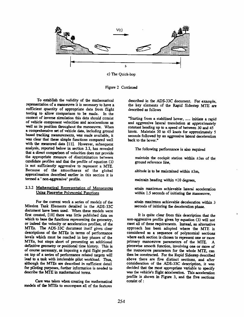
This velocity profile, shown in Figure 1, can beapplied to any of the three component axes of the

helicopter to give quick-hop (x), sidestep (y) and bob-up (z) manoeuvres, Figm'¢ 2.

S

a) The Sidestep b) The Bob.up

Figure 2 Acceleration and Deceleration Manoeuvres

253

LI-

v(t)y

$

c) The Quick-hop

Hgure 2 Continued

To establish the validity of the mathematicalrepresentation of a manoeuvre it is necessary to have asufficient quantity of appropriate data from flighttesting to allow comparison to be made. In thecontext of inverse simulation this data should consist

of vehicle component velocities and accelerations aswell as its position throughout the manoeuvre. Whena comprehensive set of vehicle data, including groundbased tracking measurements, was made available, itwas clear that these simple functions compared wellwith the measured data [11]. However, subsequentanalysis, reported below in section 3.3, has revealed

that a direct comparison of velocities does not providethe appropriate measure of discrimination betweencandidate profiles and that the profile of equation (3)is not sufficiently aggressive to represent a MTE.

Because of the smoothness of the globalapproximation described earlier in this section it is

termed a' non-aggressive' profile.

2.3.2 Mathematical Reoresentati0n Of ManoeuvresUsing Piecewise Polynomial Functions

For the current work a series of models of theMission Task Elements detailed in the ADS-33Cdocument have been used. When these models were

first created, [10] there was little published data onwhich to base the functions representing the geometry,or indeed the velocity or acceleration profiles, of theMTEs. The ADS-33C document itself gives cleardescriptions of the MTEs in terms of performance

levels which must be reached in key phases of theMTEs, but stops short of presenting an additionaldefinitive geometry or positional time history. This is

of course necessary, as imposing a rigid flight profileon top of a series of performance related targets willlead to a task with intolerable pilot workload. Thus,although the MTEs are described in sufficient detailfor piloting purposes, further information is needed todescribe the MTE in mathematical terms.

Care was taken when creating the mathematicalmodels of the MTEs to encompass all of the features

described in the ADS-33C document. For example,the key elements of the Rapid Sidestep MTE aredescribed as follows

"Starting from a stabilised hover ...... initiate a rapidand aggressive lateral translation at approximatelyconstant heading up to a speed of between 30 and 45knots. Maintain 30 to 45 knots for approximately 5seconds followed by an aggressive lateral decelerationback to the hover."

The following performance is also required

maintain the cockpit station within :t:3m of theground reference line,

altitude is to be maintained within +3m,

maintain heading within +10 degrees,

attain maximum achievable lateral acceleration

within 1.5 seconds of initiating the manoeuvre,

attain maximum achievable deceleration within 3

seconds of initiating the deceleration phase.

R is quite clear from this description that thenon-aggressive pmfde given by equation (3) will notmeet aU of these requirements. Instead, an alternativeapproach has been adopted where the MTE is

considered as a sequence of polynomial sectionswhere each section is chosen to represent one or moreprimary manoeuvre parameters of the MTE. A

piecewise smooth function, involving one or more ofthe manoeuvre parameters for the whole MTE, canthen be constructed. For the Rapid Sidestep describedabove there are five distinct sections, and afterconsideration of the ADS-33C description, it was

decided that the most appropriate variable to specifywas the vehicle's flight acceleration. This accelerationprofile is shown in Figure 3, and the five sectionsconsist of :

254

i) a rapid increase of lateral acceleration to a

maximum value of _/max after a time of taseconds,

ii) a constantaccelerationsectionto allowtheflight

velocitytoapproach itsrequiredmaximum value,Vmax,

iii)a rapid_alsitionfrom maximum accelerationto

maximum decelerationVm in in a time of tdseconds,

iv) a constantdecelerationtoallowthe flightvelocitytobe reducedtowardszero,

v) a rapid decrease in decelerationbringing thehelicopterback tothe hover.

_TrnAx -

7

o

u

<

Vmln

ta

i

, kl

tl / "

Time (s)

/"Hgure 3 Piecewise Polynomial Representation of an

Acceleration Profile for a Rapid SidestepMTE

The controlstrategyand statetime histories

which this profileproduces will be discussed in

section3.3.The valuesof Vmax and _/minareinputs

(effectivelydependenton thevehiclebeingsimulated)

whilstin orderto ensurethatthe performancelimits

aremet,thevaluesoftaand tdaresetsuch that

ta< 1.5s and td<3.0s

Referring to Figure 3, the times t l and tm arecalculated to give

tl tm

J V(t) dt - Vmax and ! _'(t)dt - 0t

where Vmax is the maximum velocity reached during

the manoeuvre and from Reference 1 is required to besuch that 30 < Vmax < 45 knots. The transient

acceleration profiles are expressed a cubic functions

of time so that, for example in the nmge t<ta,

_(t)= [-2 (_)3 + 3 (t-_) 2] Vmax (4)

The other performance requirements are readilyincorporated into an inverse simulation. For example,heading can be constrained to be constant, whilstconstant altitude flight along a reference line is

guaranteed by ensuring that the off-axis componentsof velocity are set to zero. The only feature of theRapid Sidestep MTE as given in ADS-33C which hasbeen disregarded is the necessity to maintain themaximum velocity, lateral flight state between theacceleration and deceleration phases of the manoeuvre

for approximately 5 seconds. For the purposes offlight trials this 5 second period may yield usefulinformation on the handling characteristics of the

vehicle - for example, poor handling might beindicated if any transient motions present in the

vehicle's response do not diminish rapidly once thesteady flight state had been attained. For inversesimulation this 5 secondperiodwould be modelled as

a constant velocity, straight line flight path, and thecalculatedvehicleresponsewould consistsimplyof a

series of identical trim states. This will yield littleuseful information, and this phase of the MTE hasthereforebeen ignored.

Developed in this way, in order to capture theaggressive nature of the MTE, the piecewise

representationis termed an 'aggressive profile'. A

comparison of sidestep manoeuvres generated by bothaggressive and non-aggressive profiles can beobtained by differentiating equation (4) to obtain the

acceleration for the global polynomial def'mition.This comparison is shown in Figure 4 from which it isapparent that if the manoeuvre is to be performed inthe same time for both cases, then the peakacceleration encountered will be significantly greaterin the global polynomial case. This effect is discussedfurther in section 3.3.1.

Ib _/ lbTime (s)

.rt" /

Aggressive Profile

-_ Non-aggressive Profile

Figure 4 Comparison of Acceleration Prof'des forRapid Sidestep MTE

Not all of the MTEs described in Reference 1

can be converted in quite such a straightforwardmanner as the Rapid Sidestep described above. For

255

example, the Pull-up/push-over which is describedonly in terms of the load factor profile requires the

imposition of additional criteria to complete the flight-path definition. In creating the mathematical

representations of the MTEs used here, certainassumptions have been made based mainly on theexperience gained modelling the earlier NOE

manoeuvres. As further information on flight testingusing MTEs becomes available it will be possible tovalidate these models, and improve them as necessary.

3. Inverse Simulation a_ a Tool for HandlinfOualities _[

In this section several approaches to handlingqualities assessment through inverse simulation arediscussed, and some examples are presented toillustrate their effectiveness. Comparisons are madebetween the results obtained for two configurations ofthe same helicopter, a battlefield/utility type (based

on the Westland Lynx). The baseline configuration,Helicopter 1, has a mass of 3500 kg, and a rotor whichis rigid in flap. The second configuration, Helicopter

2, differs from Helicopter 1 in that it has a fullyarticulated rotor and is 500 kg heavier, the increase in

mass causing the centre of gravity to shiftapproximately 7.5cm aft of a position directly belowthe rotor hub. The aim here was to create two

configurations with a high degree of similarity (bothhave identical fuselage and rotor aerodynamiccharacteristics, for example), but with differingperformance and agility characteristics.

3.1 Confirmation of Helicopter performance whenFlvin_ Missi¢0 Task Elements

Although ADS-33C [1], is directed towardshandling qualities, it is unavoidable that the MissionTask Elements that form part of the aggressive taskrequirements contain a significant element ofperformance related criteria which refer to theparticular configuration being flown. Therefore, the

ability to confirm that an existing or projected designcan satisfy the criteria, in a performance sense, overthe full range of MTEs is of some significance.Section 2.3 discussed how the descriptions of MTEsgiven in Reference 1 may be converted to a flight pathtrajectory defmition. When the definition is complete,the availability of an inverse simulation enables a

range of performance criteria of candidate helicoptersto be investigated against configuration parameters -such as control limits, rotor stiffness and installed

power. While it is recognised that these criteria maynot be the primary considerations which drive thedesign of the helicopter, inverse simulation canquickly establish the performance limitations of agiven design over the full range of MTEs. The

following example has been chosen to illustrate thisfacility.

3.1.1 Comparison of Performance in the TransientTurn MTE

This particular MTE is of interest as, in order tofly it, high roll rates and large roll angles areinevitable, and the parametric differences between thetwo configurations will have a marked effect on the

control time histories generated by inverse simulation.

a) Mathematical Description of the Traosient TurnMTE

The main features of this MTE, as described in

Reference 1, are that a 180 degree heading changeshould be completed within 10 seconds of initiatingthe manoeuvre at a flight velocity of 120 knots.

Previous experience of creating models of turningmanoeuvres [10] has indicated that the mostappropriate parameter to specify is the vehicle turnrate. Following the technique used to model the

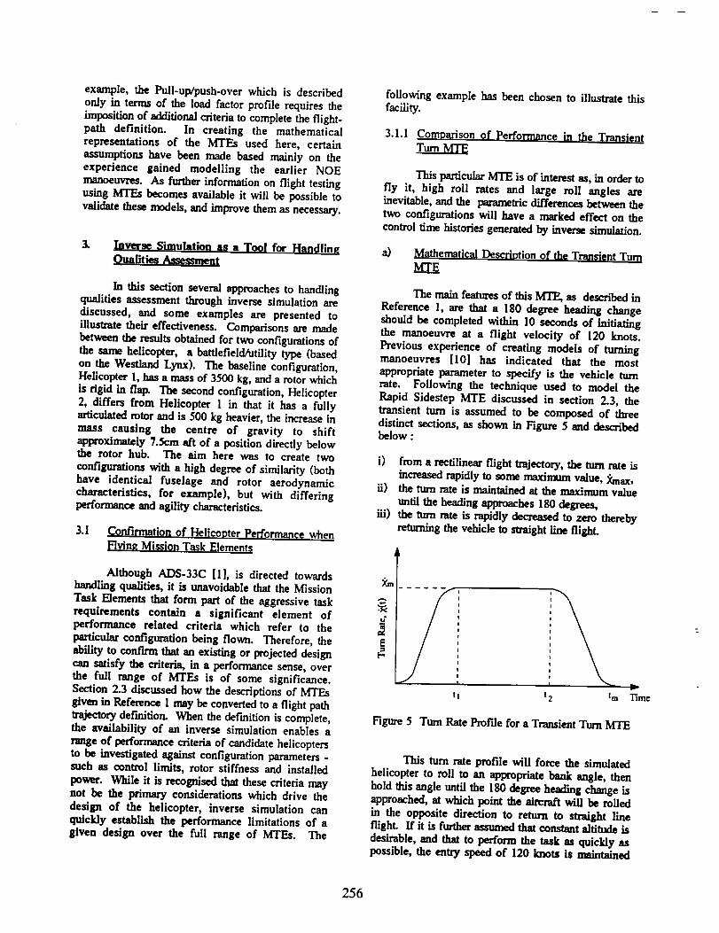
Rapid Sidestep MTE discussed in section 2.3, thetransient turn is assumed to be composed of threedistinct sections, as shown in Figure 5 and describedbelow :

i) from a rectilinear flight trajectory, the _ rate is

increased rapidly to some maxinmm value, _ax,ii) the turn rate is maintained at the maxinmm value

until the heading approaches 180 degrees,

iii) the turn rate is rapidly decreased to zero therebyreturning the vehicle to straight line flight.

.'K

[-

tl t 2 tm

7..-

T'Lme

Figure 5 Turn Rate Prof'de for a Transient Turn MlrE

This turn rate profile will force the simulated

helicopter to roll to an appropriate bank angle, thenhold this angle until the 180 degree heading change isapproached, at which point the aircraft will be roiled

in the opposite direction to return to straight lineflight. If it is further assumed that constant altitude is

desirable, and that to perform the task as quickly aspossible, the entry speed of 120 knots is maintained

256

._. 20.

18.

1G.

14.

" 12.

100

_., 10.

-sJ

.-, IOO.

_ 5o.

-- -50.

-100.

/- \

Time (s)

lO

Tune (s)

--, o_

ul w2.I

•_ -4.

-6.

¢%3

8c_

oo

B0.

._ G0.v

Time (s) "_. _ 40.

-20.

Time (s)

$ 10I !

'4 ......... -../

, \

Time (s)

_o

Tmme (s)

Helicopter 1

....... Helicopter 2

Figure 6 State and Control Time Histories from Inverse Simulation of a Transient Turn MTE

throughout, then the turn rate profile shown in Figure5 is sufficient to obtain the required mathematicalrepresentation. A full description of how the flightpath can be obtained from the turn rate profile andairspeed is given by Thomson and Bradley, [10], butthe basic principle involves varying the maximumturn rate, Xmax, until the manoeuvre is completed

within 10 seconds, and the heading change(effectively the area under the turn rate profile inFigure 5) is 180 degrees. This situation is reached

when the turn radius is 155m and the resultingmaximum normal load factor is 2.75. Note that the

fraction of the manoeuvre spent in the entry and exittransients must also be specified and in this case a

value of 15% was chosen after examination of flighttest data from similar manoeuvres [8].

b) Inverse Simulation of Two Config_urations

_ring Transient Turn MTE - Control $_ategv

Having defined the helicopter configurationsand specified the manoeuvre, it is possible to performinverse simulations of the two configurations flying it.The control time histories generated are shown in

Figure 6, from which the overall control strategy canbe deduced. The manoeuvre is initiated by a pulse inlateral cyclic to roll the aircraft,note that there is littledifference in the amount required between the twoconfigurations. As the aircraft rolls, also shown inFigure 6, collective (and hence thrust) rmmt be addedto maintain altitude. There is also a forward motion

of the longitudinal stick (denoted by negativelongitudinal cyclic) to maintain constant forward

speed. The manoeuvre is performed without sideslipand tail rotor collective is used to ensure this

condition is met. The initial pulse in lateral cyclic isopposed by a similar pulse in tallrotor collective

257

which then increases beyond its level flight trimposition to offset the extra torque produced byincreased main rotor collective. The main differencesbetween the time histories of the two aircraft lie in the

collective and longitudinal plots. The baselineconfiguration, Helicopter 1, requires less collectivefirstly because it is lighter, but one must also considerthe effect of shifting the centre of gravity aft of therotor hub. This produces a nose up pitching momentwhich must be countered by forward stick if velocityis to be maintained, which explains the 2 degrees ofextra forward longitudinal cyclic required by the lessagile configuration, Helicopter 2. The longitudinaltilt of the thrust vector is in addition to the lateral tilt

required for rolling, and hence is a contributoryfactory in the 2.5 degrees of extra collective requiredby Helicopter 2. Examination of Figure 6 shows thatthe roll angle history which was suggested by themanoeuvre definition is obtained, and the maximum

bank angle reached was approximately 70 degrees,with roll rates of approximately 70 degrees/secondencountered in the transients.

c) Inverse Simulation of Two ConfigurationsFlying Transient Turn MTE - Confirmation of

performance

The advantage of using inverse simulationbecomes apparent when it is realised that thecollective limit of this configuration is 20 degrees.Consequently, on examination of the collective timehistory in Figure 6, it is clear that Helicopter 2 is closeto the limiting case for this manoeuvre. It thenfollows that the limiting case for various aircraft

masses and centre of gravity positions could beobtained by repeated inverse simulation of the

manoeuvre thereby allowing the aircraft configurationenvelope for this MTE to be derived. This type ofinvestigation may be extended to include a range ofMTEs and configurational parameters.

For performance comparisons the applicationof inverse simulation is clear cut. Given the

availability of a helicopter model of appropriatevalidity, it is sWaighfforward to measure comparativecontrol margins and control activity for a given set ofmanoeuvres. Experience has shown that the facilitiesoffered by flight mechanics models such as HGS areadequate for such investigations. Therefore theremaining task is to compile a suite of validatedmanoeuvre definitions - and although several of thedescriptions of Reference I0 have been validated

against flight data there are several manoeuvres forwhich flight tests are required to provide practicalvalidation. The conclusion to be drawn is that while

performance comparisons of this kind arestraightforward to conduct, the handling qualitiesinformation that it can provide is limited and likely toremain so.

3.2 The Handling Qualities Index

One of the earliest applications of inversesimulation was an attempt to quantify the agility of a

given helicopter configuration through an AgilityPerformance Index (API) [12]. The difficulty ofproducing a general definition of the term agility iswell known [4] but the API was based on the conceptof installed agility, that is, it was dependant on theparticular configuration of the helicopter andindependent of any pilot model. This independence ofa pilot model is a feature of the inverse formulationsince it generates a precise piloting task and leaves noscope for other than ideal piloting of the helicopter.The API of a helicopter for a given manoeuvre wasdetermined from the formula:

ng

API = Z qf0 = f(xi (t)) dt +i=l

n¢

]=l

where tm is the time taken to complete the manoeuvre,

qi and rj are weighting constants related to state i andcontrol j. The integers ns and nc are the number of

states and controls to be included in the performance

index. The functions f(xi(t)) and g(uj(t)) wereselected to penalise large state and control deviationsduring the manoeuvre: for example,

_- I.'(t)'xit_= ]2._f(_q (t))

LXi m= xi_,,

where Xitrim is the value of state i, in the steady flight

condition at the entry to the manoeuvre, and Ximax is

the maximum value of the state encountered duringthe manoeuvre. Using this definition low values ofAPI (i.e. small control and state displacements) will

imply good agility. The obvious difficulty with such

an approach is the appropriate choice of the weights qi

and rj and, in practice, zero or unity were commonlyemployed in comparative studies of differenthelicopter configurations on the basis of whether it

was felt that those quantities were significant or notin a particular manoeuvre. Nevertheless, despite thissimplified approach, the work established theprinciple whereby different helicopters could be

comparatively assessed for their agility over a rangeof standard manoeuvres by a reproducible simulationstudy.

Having established the principle for agilitystudies, it is attractive to consider a similar approachfor handling qualities and def'me a Handling Qualities

258

Index (HQI) using a similar form to that in equation(5). It may be necessary to include other terms suchas auto- and cross-correlations of the control

responses but from the whole of the attitude, rate,velocity, acceleration and control information, itshould not be unreasonable to expect that anappropriate balance of the coefficients in the

formulation of the HQI could produce a formulawhich reflects, in large measure, an assessment of

handling qualifies. Unfortunately, the question offinding the values of the coefficients necessary toachieve the appropriate balance is impracticable - just

as in the case of the API. Therefore, althoughconceptually attractive and demonstrable in principle,the HQI falls at the present time because of the lack of

essential knowledge about the coefficient values, andif it were to be seriously considered for developmentin the future then an extensive validation programmewould be needed to establish its credibility.

3.3 Ouickness Parameters

In addition to the calculation of the time

responses of the control displacements, inversesimulation of a given manoeuvre calculates the

responses of the full range of kinematic variables.

Included in this information, are the time-histories of

roll rate p and roll angle @. so that when a Rapid

Sidestep manoeuvre is simulated according to thetranslation velocity profile defined by Figure 3 it is a

,,-, 40.

20.

-20

-41

straight forward matter to calculate the quickness

parameter chart Ppk/_4_pk against L_4bmin in a manner

described by the ADS-33C document, section 3.3.

The time histories of p and _ shown in Figure 7 for

the sidestep manoeuvre with ta = 1.5s, td = 3s, Vma x =

35 Knots, Vmax = 5m/s 2 and "_min = -5 m/s 2, are

obtained from the inverse simulation of Helicopter 1

for the Rapid Sidestep using the aggressive profiledefined by Figure 3. They are annotated to show the

calculations of the quickness parameters of the main

pulses of roll rate. Fh'st there is the roll into the

manoeuvre then, at about the midpoint, there is a roll

in the opposite direction to bring the rotor into a

position to decelerate the helicopter, and f'mally thereis a roll back to the level, trim, position. The attitude

quickness parameters corresponding to this data and

data from a variety of similar manoeuvres (obtained

by varying the parameters used to def'me the MTE

model) are shown in Figure 8 and it can be seen that

the values mainly lie in the Level 1 region.

--" 20.

o

-40

The corresponding control displacement time-histories are shown in Figure 9 but it should be borne

in mind that the attitude quickness parameters havebeen calculated solely as a result of a defined

manoeuvre so are not, in the context of inversesimulation, necessarily an appropriate measure of the

2.O,

.!_. 3O.9 PpL

2--'8" " 0.953 L_pk

,o '.°Tune (s)

@.@.

I_t . -33.3• t_ .-_-- - 0.595

OoO

m

o

LEVEL I *a

LEV_

ILEVEL 3

x

L_ min(deg)

• Vmm " 35 kno_ I, - I.Ss, I4 - 3,0s, _'-m,_a " ± 6 m/s 2

• V_-351moet, tl-l.5s , M-3.0s, Vrrm_n.±5m/s 2

* Vnm " 35 knout, t. - [.5s, td " 3.0s, _/max/mmn " ± 4 nVs 2

x Vmu-50knots, _,-I.Ss, td-3.0s, Vnax_n.±Sm/s2

o V,rm-]Sknoet, tt'l.Os, _-2.0s, "_nm/_.±4n_,s 2

* Vmex - 35 knots, (, - I.Os, [d " 2,0s, _/_a " _ 5 m/s 2

Figure7 Calculation of Roll Quickness from

InverseSimulationofHelicopterI Flying

a Rapid SidestepMTE

Figure 8 Roll QuicknessChartforHelicopter 1 from

Inverse Simulation of Rapid Sidesteps

259

.... 2.exo0j

0_D

ff;>

o -2

m

0.5.

__ 0.0

° ,.J -0.5

-I .0.

q -1 .5.

"_ 2.

u

J

-I.--2.

-3.

4.

v

o_ 2

0

-2

Time (s)

rate, p, and this similarity suggests that

integral of 01c :

t

OIc - 101c(t) dtd

Olc , the

relates to the value of the bank angle so that a control

quickness parameter 01cpk/ A O1Cpk may be the

equivalent parameter, and when plotted against AOlc ,

would give a chart equivalent to that used to plotattitude quickness. The manner of calculation isidentical to that of the attitude quickness as illustratedin Figure I0. That this quantity is a useful measure toinvoke from the inverse simulation method isdiscussed in more depth in section to follow.

2,

""-_N b _ o

Tune (s) _ -z

Figure 9 Control Displacements for Helicopter 1Flying a Rapid Sidestep MTE

= 1.___s= i.o2Olcm m 1.47

= -1._A4.0.9s. -ll -1.47

Olca_ -1.-"9 " 1.1 Olemi_

T'L,_ (s)

lb

handling qualities of a particular configuration. Theseissues are further elaborated in sections 3.3.1 and3.3.2 but before leaving the current discussion it is

opportune to give some initial attention to the outputof the inverse analysis - that is the set of control time

histories - and pose the question of how to process itto afford some measure of handling quality or pilotworkload. The lateral cyclic control displacement,01c, certainly does not have the characteristics of the

bank angle so that the parameter ()lcpk/A01cpkiS

unlikely to be useful - and indeed experimentation hasshown this to be the case. In fact, it may be observedthat the pulses of lateral cyclic away from the trimposition are of a similar character to the pulses of roll

Figure 10 Calculation of Lateral Cyclic QuicknessParameter from Inverse Simulation of

Helicopter 1 Hying Rapid Sidestep MTE

3.3.1 Influence of MTE Mode l

In this section we return to the issues raised

above regarding the calculation of quicknessparameters for predef'med manoeuvres. The f'LrStaimof this discussion is to qualify the observations madeon previous occasions that the details of the

manoeuvre profile defmition have not appeared to besignificant. When faced with the requirement tospecify the velocity profile of a sidestep MTE, for

260

example, it is natural, as described in section 2.3.1

above, to write down in the first instance the non-

aggressive profile, since it is the computationallysimplest description. It gives a smoother change in

acceleration than the aggressive profile described in

section 2.3.2 as has been illustrated in Figure 4.

When this manoeuvre is simulated using the

Helicopterl configuration, the attitude quickness

parameters vary significantly from those derived

from the more sharply executed aggressive manoeuvre

and lie mainly in the Level 2 region as is shown in

Figure 11. Here then is a further criterion by which to

select a manoeuvre description:- if it is to be used forhandling qualities studies within the ambit of ADS-

33C then a description must be employed which sets

the manoeuvre in the Level 1 region. The attitudequickness parameters have discriminated

quantitatively between the aggressive and non-

aggressive profiles, confirming the quantitativediscrimination noted earlier.

D_L2.0

(/5) I .Ig

| .0,

0.11.

0.0

LEVEL I

ILEVEL 3

ib

I

--"7",,

ab =b _ sb eb

_b =,a(deS)

• ha" 1Is

• ha" II s

* he'10s

x ha-9s

Vsm - 35 Imms

Figure 11 Roll Quickness Chart for Helicopter l

from Inverse Simulation Using Non-

aggressive Sidestep Profile

3.3.2 Influence of ConfiRuration

Now consider the effect of altering thehelicopter's configuration to a less agile version. The

Helicopter 2 configuration of the vehicle has more

weight and significantly reduced rotor stiffness.

Applying the same manoeuvre to it produces, as seen

in Figure 12, almost identical attitude quickness

values - in fact occurring in closely positioned pairs.

This result is typical of many simulations which have

been conducted and which lead to the initially

surprising conclusion that the attitude quickness

parameters are largely independent of theconfiguration used in the inverse simulation. A little

reflection will show that this effect is not unusual

since the roll rates and attitude angles through a

manoeuvre are largely dictated by the manoeuvre

profile itself and one should expect some agreement

forotherthangrossconfigurational changes.

ppk

L_bpk

(/s)

1.st

1.0.

0.5.

0.0

÷o

tJ

LEVEL 1 _

LEVE_

_'o °'It

LEVEL 3

ib 2b 3b 4b 5b

_b rain (deg)

Helicopter I

%M_n_. =*Sm/s 2 _ h'l.Ss, td-3.0sVmaa/min = ± 4 m/s 2 I

; *ma_mm'±Sm/s2 } le'l'0s' _d=2.0sVn'm/min = '_ 4 m/s 2

Helicoplef 2

V,,w,/mm " ± 5 n_s 2Vmmamin " "_ 4 nVs 2 } la " I.Ss, _1" 3.01

: V'au_'_n'+SnVs2 } h" 1.0s. _-2.0s_/mu/mia " :I: 4 m/s 2

Vain - 35 kno_ in all cases

Figure 12 Roll Quickness Chart for 2 Configurations

from Inverse Simulation of Rapid SidestepMTE

However, the control quickness is influenced

by the variation in configuration. Figure 13 shows

quite clearly that it increases significantly for the

Helicopter 2 configuration, representing the additionaleffort required by the pilot to drive the inferior

configuration through the same manoeuvre. The

control quickness parameter, as defined in Section 3.3,

is remarkably effective in discriminating betweendifferent configurations.

261

Olcpk

el_pk

(/s)

1.4.

1.3.

1.2

I,I

1.0.

O.S

0

Figure 13

a

o

o

%

xx

x xx

o_s _"o :s 2:0 2"5

,xOt_(degs)

R Helicopter 1

a Helicopter 2

Lateral Cyclic Quickness Chart for 2Configurations from Inverse Simulation of

Rapid Sidestep MTE

0lcpk"

_|¢pk

(/s)

1.4

1.3_

1.2,

1.1.

l.O.

o

Level_.3 _ 5,

Leve_ x

LevelI

0.$:s 2"o

A6")i_ (deg.s)

Figure 14 Lateral Cyclic Quickness Chart with

Suggested Workload/Handling QualitiesBoundaries

2_s

3.4

These simple illustrations suggest a procedureto be followed when using inverse simulation for

handling qualities studies. One must use the

requirements, such as ADS-33C, in an inverse

manner. F'Lrstthe manoeuvre must be refined until it

satisfies the level of handling demanded by the

requirements regarding attitude quickness, then

various configurational changes can be compared by

examining the corresponding control quicknessvalues. An increase in the value of the control

quickness indicates an increased work load and hence

a worsening of the handling qualities. In addition to

there being a relative measure it may be possible, as

indicated speculatively on Figure 14 to identifyregions in the control quickness chart which

correspond to particular levels of pilot workload orhandling rating.

4. Conclusions

The potential of three approaches for

employing Inverse simulation to assess handling

qualities have been discussed. Two of them, the

Handling Qualities Index and the performancecomparisons have been shown to have limited

potential while the third, the use of attitude and

control quickness parameters in a dual relationship,promises useful exploitation.

Two general conclusions may be made aboutthe current state of inverse simulation:

(a) Cm'rent mathematical models, such as FIGS, areadequate for basing inverse flight mechanicsstudieson.

(b) Flight tests should be made to validate the flight-path models currently being developed.

The main conclusion of this work resides in the

significance of the quickness parameters inassociation with inverse simulation.

It is important to emphasise that these

investigations have indicated a practical criterion for

deciding on the appropriate modelling of an MTE for

inverse simulation. That is, the model must generateattitude quickness parameters which lie in the Level 1region. Moreover, the choice of manoeuvre model is

practically independent of helicopter configuration-Therefore, referring to the conditions set out in the

introduction, this is the sense in which manoeuvresmust be representative.

262

Theapproach has been taken further and it has

been shown to be possible to define a control

quickness parameter which can discriminate betweendifferent helicopter configurations flying the same

manoeuvre. While it is acknowledged that the choice

of definition for the control quickness may require

future development, it is clear from the work done sofar that this general approach can potentially extend

the scope of simulation in demonstrating compliance

with handling qualities requirements. It does appear

from this work that in using quickness parameters theconditions are sufficient for the successful use of

inverse simulation providing that it is realised that it is

the control quickness that is the determining factor inthe assessment.

Acknowledgements

The authors wish to thank The Royal Societyfor their continued support of this work. The co-operation Dr Gareth Padfield of the Defence ResearchAgency, RAE Bedford, is also appreciated, withparticular reference to the use of look-up tables andhelicopter configurational data.

.

Z

.

4.

References

Anon, "Aeronautical Design Standard, HandlingQualities Requirements for Military Rotorcraft."ADS-33C, August 1989.

Bradley, 1L, Padfield, G.D., Murray-Smith, DJ.,Thomson, D.G., "Validation of HelicopterMathematical Models." Transactions 9f the

Institute of Measurement and Control, Vol. 12,No. 4, 1990.

Thomson, D.G., Bradley, R., "Development andVerification of an Algorithm for HelicopterInverse Simulation." Vertica, Vol. 14, No. 2, May1990.

Whalley, M.S., "Development and Evaluation of

an Inverse Solution Technique for StudyingHelicopter Maneuverability and Agility." NASATM 102889, July 1991.

, McKillip, 1LM., Perri, T.A., "Helicopter FlightControl System Design and Evaluation for NOEOperations Using Controller InversionTechniques." 45th Annual Forum of theAmerican Helicopter Society, Boston, May 1989.

. Padfield, G.D., "A Theoretical Model forHelicopter Flight Mechanics for Application toPiloted Simulation." Royal AircraftEstablishment, TR 81048, April 1981.

. Thomson, D.G., "Development of a GenericHelicopter Mathematical Model for Applicationto Inverse Simulation." University of Glasgow,Department of Aerospace Engineering, Internal

Report No. 9216, June 1992.

. Thomson, D.G., Bradley, R., "Modelling andClassification of Helicopter CombatManoeuvres." Proceedings of ICAS Congress,Stockholm, Sweden, September 1990.

. Taylor, C.D., Thomson, D.G., Bradley, R., "TheMathematical Definition of Helicopter Take-offand Landing Manoeuvres for OffshoreOperations." University of Glasgow, Departmentof Aerospace Engineering, Internal Report No.9243, October 1992.

10. Thomson, D.G., Bradley, R., "The Use of InverseSimulation for Conceptual Design." 16thEuropean Rotorcraft Forum, Glasgow, September1990.

11. Thomson, D.G., Bradley, R., "Validation ofHelicopter Mathematical Models by Comparisonof Data from Nap-of-the-Earth Flight Tests andInverse Simulations." Paper No. 78, Proceedingsof the 14th European Rotorcraft Forum, Milan,Italy, September 1988.

12. Thomson, D.G., "An Analytical Method of

Quantifying Helicopter Agility." Paper 45,Proceedings of the 12th European RotorcraftForum, Garmisch-Partenkirchen, FederalRepublic of Germany, September 1986.

263