N87-11722

APPLICATION OF THE GENERALIZED REDUCED GRADIENT METHOD

TO CONCEPTUAL AIRCRAFT DESIGN

Gary A. Gabriele

Lockheed-Georgia Company

PRECEDING PAGE BLANK NOT FIEMI_

65

https://ntrs.nasa.gov/search.jsp?R=19870002289 2018-07-01T18:10:57+00:00Z

AIRCRAFT DESIGN PHASES

The complete aircraft design process can be broken into three phases of in-

creasing depth: conceptual design, preliminary design, and detail design. Con-

ceptual design consists primarily of developing general arrangements and selecting

the configuration that optimally satisfies all mission requirements. The result

of the conceptual phase is a conceptual baseline configuration that serves as the

starting point for the preliminary design phase.

The conceptual design of an aircraft involves a complex trade-off of many inde-

pendent variables that must be investigated before deciding upon the basic con-

figuration. Some of these variables are discrete (number of engines), some repre-

sent different configurations (canard vs conventional tail) and some may represent

incorporation of new technologies (aluminum vs composite materials). A particular

combination of these choices represents a concept; however there are additional

variables that further define each concept. These include such independent vari-

ables as engine size, wing size, and mission performance parameters, which must be

selected before a particular configuration can be evaluated. Generally, these

additional variables are chosen to optimize each concept before selecting a final

configuration.

Missio n _'_

equirements ,/!

[ Conceptual __.__.{/_onceptual_Design / k,,,. Baseline J

/• Optimization _ _

"1

• Parametric Preliminary /

• 1st Level Analysis Design J• Sophisticated

Analysis

• Multi-Discipline

• Optimization

Advanced

Design

• General Arrangement & Performar_ce

• Representative Contours

• General Internal Arrangement

AIIocated__ Baseline j'

Detailed

Design

Project

Design.

• System Specifications

• Detail Contour

• Internal Arrangement

__Production"_Baseline J • Part

Drawi.g

IProduction

& Support

66

OPTIMAL VEHICLE SELECTION BY PARAMETRIC DESIGN

The principal analysis tool used during the conceptual design phase is the

sizing program. At Lockheed-Georgia, the sizing program is known as GASP

(Generalized Aircraft Sizing Program). GASP is a large program containing

analysis modules covering the many different disciplines involved in defining

the aircraft, such as aerodynamics, structures, stability and control, mission

performance, and cost. These analysis modules provide first-level estimates

the aircraft properties that are derived from handbook, experimental, and his-

torical sources.

To make a run of the sizing program, the engineer develops a data set defin-

ing the fuselage geometry, the mission profile, a candidate propulsion system,

the general arrangement of the components, the extent of new technologies to be

incorporated into the design, and the values for the independent design variables.

The sizing program provides a complete weight breakdown of the airplane, aerody-

namic properties, mission and airport performance, center of gravity ranges,

and cost data.

Mission Inputs

M

Installed Engine I

Data I

co

InputAssumptions• Wing Loading

• Cruise Altitude

• Cruise Power %

• Aspect Ratio

• Sweep

Tail Volumes

Tail Arms

Flap Span

Flap Chord

BaselineGeometry

I_,_,

E-_'3

_r..° -_ _ _,

I) o, Illl

--I G ) ' r !!iion FuelIField Performance _

67

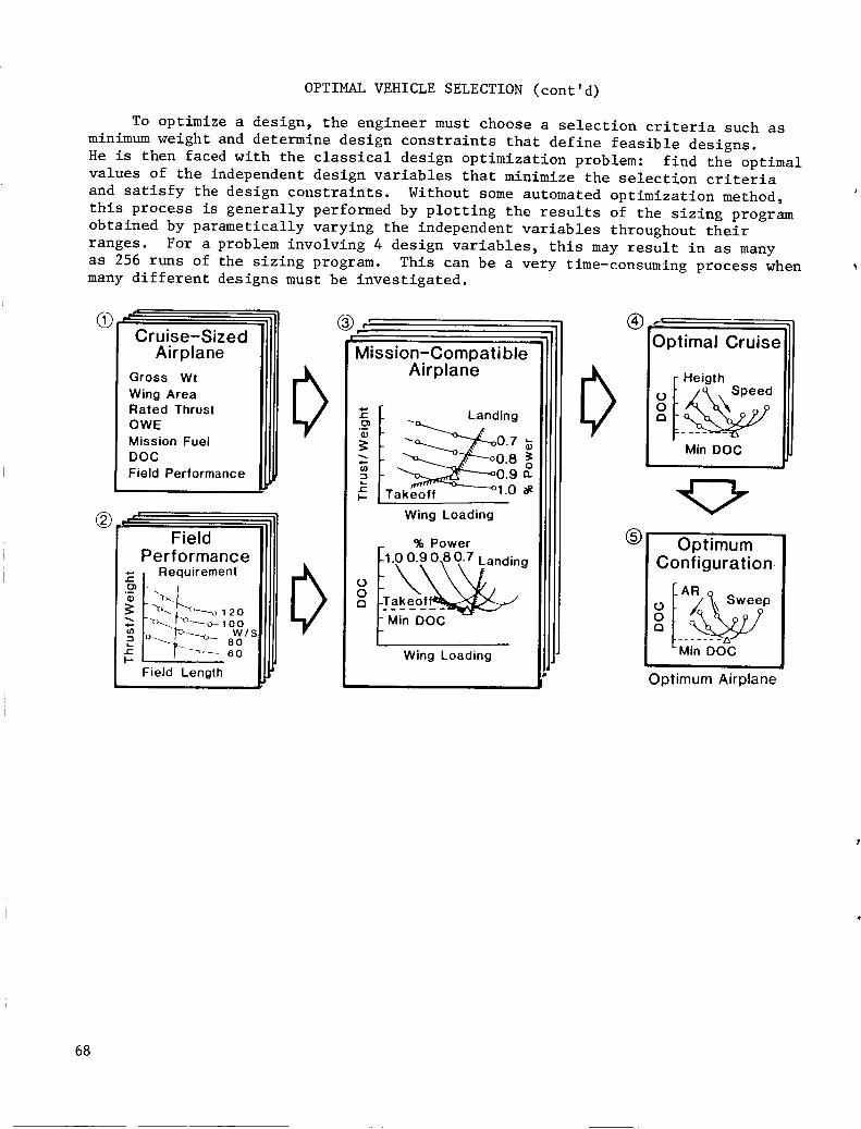
OPTIMAL VEHICLE SELECTION (cont'd)

To optimize a design, the engineer must choose a selection criteria such as

minimum weight and determine design constraints that define feasible designs.

He is then faced with the classical design optimization problem: find the optimal

values of the independent design variables that minimize the selection criteria

and satisfy the design constraints. Without some automated optimization method,

this process is generally performed by plotting the results of the sizing program

obtained by parametically varying the independent variables throughout their

ranges. For a problem involving 4 design variables, this may result in as many

as 256 runs of the sizing program. This can be a very time-consuming process when

many different designs must be investigated.

_I I ,

Cruise-SizedAirplane

Gross Wt

Wing AreaRated ThrustOWE

Mission Fuel

DOC

Field Performance

® _c =,

; Field

Performance

._ [ Requirement

.__ . I

I "XL.. r"_--_., o 1 2 0

:_ I_ -_ 80

I ooField Length

/r r

I

Mission-Compati ble

[_ Airplanef _ Landing

i I o=_ 0.9 "

Takeoff

Wing Loading

% Power[10090.807 L nJ.

._,_ , ,- _a,_olng

_ fTake _

Wing Loading

(_ .{'

Optimal Cruise

r Heigth

_ /q Speed

Min DOC

®Optimum

Configuration

AR Sweep

Optimum Airplane

68

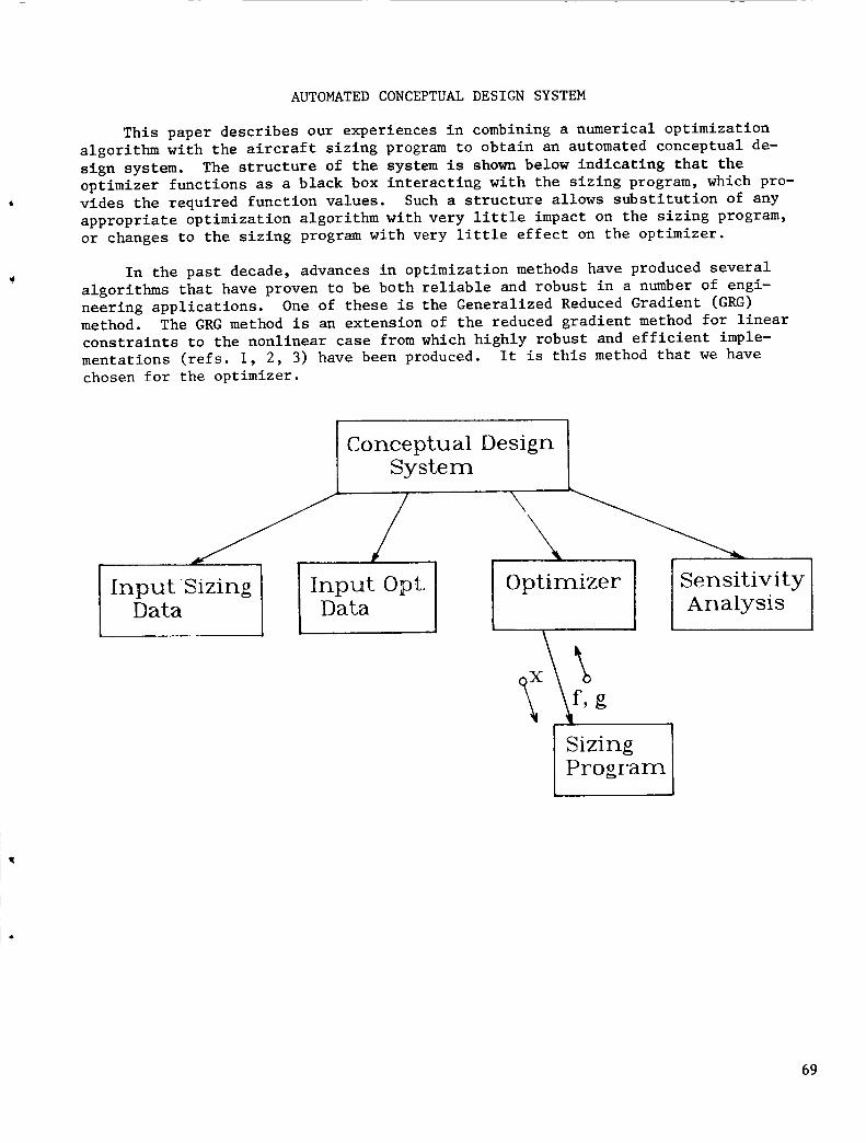
AUTOMATED CONCEPTUAL DESIGN SYSTEM

This paper describes our experiences in combining a numerical optimization

algorithm with the aircraft sizing program to obtain an automated conceptual de-

sign system. The structure of the system is shown below indicating that the

optimizer functions as a black box interacting with the sizing program, which pro-

vides the required function values. Such a structure allows substitution of any

appropriate optimization algorithm with very little impact on the sizing program,

or changes to the sizing program with very little effect on the optimizer.

In the past decade, advances in optimization methods have produced several

algorithms that have proven to be both reliable and robust in a number of engi-

neering applications. One of these is the Generalized Reduced Gradient (GRG)

method. The GRG method is an extension of the reduced gradient method for linear

constraints to the nonlinear case from which highly robust and efficient imple-

mentations (refs. I, 2, 3) have been produced. It is this method that we have

chosen for the optimizer.

Input SizingData

/Input Opt.

Data

Conceptualsystem Design l

Optimizer SensitivityAnalysis

I Program

69

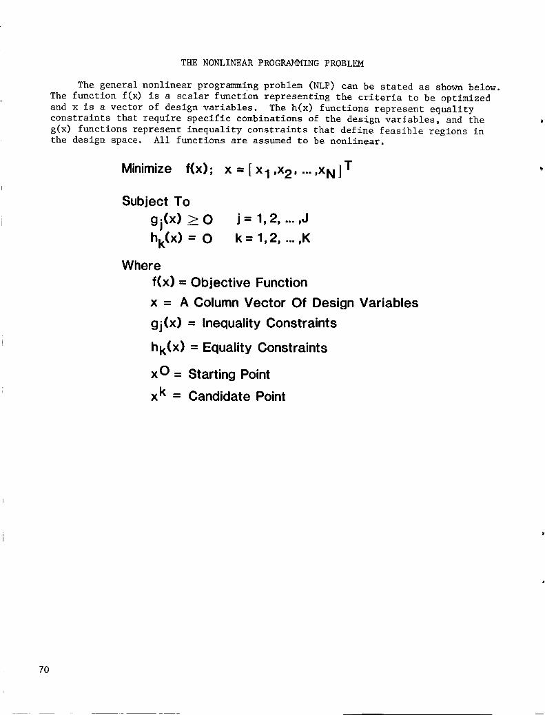
THE NONLINEAR PROGRAMMING PROBLEM

The general nonlinear programming problem (NLP) can be stated as shown below.

The function f(x) is a scalar function representing the criteria to be optimized

and x is a vector of design variables. The h(x) functions represent equality

constraints that require specific combinations of the design variables, and the

g(x) functions represent inequality constraints that define feasible regions in

the design space. All functions are assumed to be nonlinear.

Minimize f(x); x = [ Xl ,x2' --- ,XN ] T

Subject To

gj(x) > 0

hk(X) = 0

j= 1,2, ...,J

k= 1,2, ...,K

Where

f(x) = Objective Function

x = A Column Vector Of Design Variables

gj(x) = Inequality Constraints

hk(X) = Equality Constraints

xO = Starting Point

x k = Candidate Point

70

GENERALIZED REDUCED GRADIENT METHOD

The GRG method restates the NLP in the form shown below, where the vectors xL

and x 0 represent the lower and upper bounds on the design variables x. The inequality

constraints are included as equality constraints through the addition of slack vari-

ables. The parameter M represents the total number of constraints. The constraints

include only the functional constraints; variable bounds are accounted for separately

to allow for a more efficient handling of this special class of constraints.

The basic strategy of the GRG method is derived from trying to use each equality

constraint hm(X) to eliminate a design variable from the problem. However, for mostengineering problems, the constraints are too complex to allow this substitution.

The GRG method accomplishes this by employing the Implicit Function Theorem.

Minimize f(x), x = [Xl, X2,...,xNJT

Subject to

hm(x) =0

xL<<x<x U

m=l,2,...,M

Strategy:

Solve each hm(X) explicity for a Variable and Substitute

into f (x).

Problem: Not always Possible for Complex EngineeringFunctions or Simulations.

Solution: Do It Implicity.

71

DERIVATION OF THE REDUCED GRADIENT

Consider the following strategy, whose foundations can be found in the simplex

method of linear programming. Divide the design vector x into two classes, non-

basic or independent (z) variables and basic or dependent (y) variables, as shown

in the figure, where Q = N - M. The search for the optimum will occur by search-

ing in the design space of the nonbasic variables and the basic variables will be

used to satisfy the constraints. A gradient vector for this new problem can be

obtained by introducing the division of the design variables into the objective

and constraint functions and following the steps shown in equations (i) to (3).

The reduced gradient defines the rate of change of the objective function

with respect to the nonbasic variables with the basic variables adjusted to

maintain feasibility. In the presence of linear constraints, equation (3)

represents the changes necessary in the basic variables for a given change in

the nonbasic variables. Additional adjustment is necessary in the nonlinear

situation. Conceptually, the above derivation corresponds to a transformation

of the GRG problem into one having the following form:

Minimize: F(z) z = (z i' z 2''''' Zq) T

1 uSubject to: z 5 z _ z

where the basic variables y have been eliminated from the original problem by

using the constraints h m (z,y) = 0 to solve for y in terms of z. The gradient

of F(z) is represented by the reduced gradient, and the necessary equations for

y in terms of z represented by equation (3).

Divide X into two classes, dependent and independent

x = [y,z]T

Y = [Yl, Y2 ..... YM] T Dependent Variables

Z - [z, z2 ..... zQ] T Independent Variables

Calculate the first variation of f(X) and H(x) using Z and Y

df(x) - Vzf(x)rdz + Vrf(x)rdy (1)

dH(x) = VzH(X ) dz + VyH(x) dy - 0 (Z)

Solve (2) for dy

dy - [VyH(x)]-' XTzH(X ) dz (3)

Substitute (3) for dy in (1) to arrive at the REDUCED GRADIENT

Reduced Gradient VRF(z )

V.F(z) T -- Vzf(X) T - V,f(x) T VvH(x)-' VzH(x ) (4)

The Reduced Gradient defines the gradient for the new

vedzLced problem

Minimize F(z), z - [z,, z 2, ... ,z,] T

Subject to z _•z_z U

the change in Y necessary to maintain feasibility is defined byequation (3) for linear constraints.

72

CONVERGENCE PROPERTIES

A necessary condition for the existence of a local minimum of an uncon-

strained nonlinear function is that the elements of the gradient vanish.

Similarly, a local minimum of the reduced problem shown in the previous figure

occurs when theelements of the reduced gradient satisfy the conditions shown

below.

Points that satisfy these conditions satisfy the Kuhn-Tucker conditions

for the existence of a constrained relative minimum of the original NLP prob-

lem (ref. 3). An additional benefit of this method is that the Lagrange multi-

pliers are calculated in the course of calculating the reduced gradient vector.

Convergence Conditions

'<0 ifz.=z, uI I

I

> 0 if zt = z_

= 0 otherwise

i = 1, 2, 3, ... ,Q

When this conditon holds, the corresponding point X satisfiesthe Kuhn-Tucker conditions for the existence of a iocal

constrained minimum of the original probiem.

73

GENERALIZED REDUCED GRADIENT ALGORITHM

The basic steps of the GRG algorithm are given in this figure. The method

looks very much like any gradient based method, with some exceptions. The search

directions for the nonbasic variables are based on the reduced gradient vector

and initial directions for the basic variables are then calculated from equation

(3). In the calculation of the nonbasic direction any gradient-based search

method, such as conjugate gradient or variable metric, may be used.

The line search phase is also similar, except additional logic is also re-

quired to adjust the basic variables and determine when a new constraint

is encountered. The basic variable adjustment occurs in the presence of nonlinear

constraints. As we move along the search direction defined for the nonbasic vari-

ables and calculated from equation (3) for the basics, we can expect, for non-

linear constraints, that the trial points will violate the constraints. To

maintain feasibility, an adjustment of the basic variables at each trial point is

undertaken to get back to the constraint surface before evaluating the objective

function. During this adjustment the independent variables are held constant.

The line search is terminated by one of the following conditions: a relative

local minimum was located along that search direction, a new constraint was

encountered which limited the search, or adjustment of the basic variables to

maintain feasibility was not possible at some trial points.

Identify h_dependent and 1

Dependent Variables !

-_I Ca_culate Vr F(X) I

yes

Calculate Search Direction Based

on V r F(X)

Minimize Along Direction forIndependents

i_Adjust Dependent Variables _

74

DEPENDENT VARIABLE ADJUSTM/_NT

This figure depicts the adjustment of the dependent variable Yl during the

line search phase of the GRG algorithm. Here we have taken a step along the

search direction from x°. Holding the independent variable zI constant, we now

adjust Yl to get back to the constraint h(x).

ZI

f(x)=lO00)=900

75

METHODS FOR DEPENDENT VARIABLE ADJUSTMENT

A modified Newton method is usually employed to adjust the basic vari-

ables during the line search. The iteration sequence is given below, where AOis the initial inverse of Vy h(x) used at the start of the GRG iteration tocalculate the reduced gradient and t is an iteration of Newton's method.

The modified Newton method has been used in all current implementations

of the GRG algorithm. This is due primarily to the substantial savings in com-

putation time obtained by avoiding successive reformulations of the Jacobian

inverse. However, the major drawback of the method is that it does not possess

the convergence rate of the classical method obtained by evaluating the Jacobian

and its inverse at every Newton iteration. Poor convergence of the Newton method

can lead to insufficient progress being made during a line search, which may

hinder convergence of the algorithm to the optimal solution.

Two factors that have a major influence on the convergence are the approxima-

tions to the basic variables during the line search and the inaccuracies of using the

inverse AO. Suggestions for improving the former have appeared in Lasdon (ref. 2),

and Gabriele and Ragsdell (ref. 3), and both offer improvements in convergence.

Techniques for improving the inverse A0 have appeared in the literaturefor solving nonlinear systems of equations. Broyden's method (ref. 4) is one of

these methods and is summarized below. This method is used in our implementationof the GRG algorithm.

MODIFIED NEWTON METHOD

yt+l= yt _ Ao H(z k, yt )

z k = fixed values of independents

A o = initial inverse of V H(x) used in calculating Vrf(x )

BROYDEN'S METHOD

The inverse Jacobian matrix A is updated at each iteration by

A T TAi+ I=A_-( i+,v -pfil)piAi/(pl TAivl)

v i = H(z k, yt+1 ) _ H(z k, yt )

Pt = --AL H( zk, yt )

t+l yty = + s,p i

76

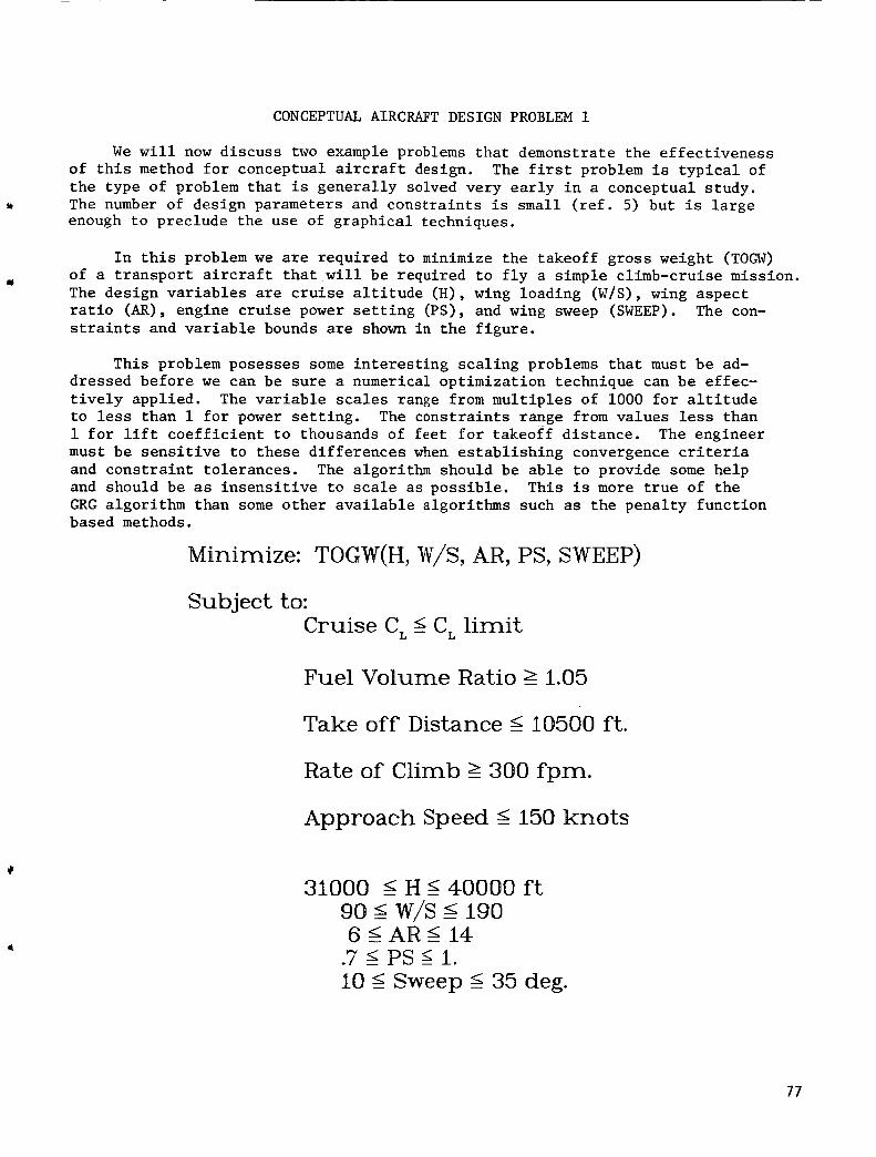
CONCEPTUAL AIRCRAFT DESIGN PROBLEM i

We will now discuss two example problems that demonstrate the effectiveness

of this method for conceptual aircraft design. The first problem is typical of

the type of problem that is generally solved very early in a conceptual study.

The number of design parameters and constraints is small (ref. 5) but is large

enough to preclude the use of graphical techniques.

In this problem we are required to minimize the takeoff gross weight (TOGW)

of a transport aircraft that will be required to fly a simple climb-cruise mission.

The design variables are cruise altitude (H), wing loading (W/S), wing aspect

ratio (AR), engine cruise power setting (PS), and wing sweep (SWEEP). The con-

straints and variable bounds are shown in the figure.

This problem posesses some interesting scaling problems that must be ad-

dressed before we can be sure a numerical optimization technique can be effec-

tively applied. The variable scales range from multiples of i000 for altitude

to less than i for power setting. The constraints range from values less than

i for lift coefficient to thousands of feet for takeoff distance. The engineer

must be sensitive to these differences when establishing convergence criteria

and constraint tolerances. The algorithm should be able to provide some help

and should be as insensitive to scale as possible. This is more true of the

GRG algorithm than some other available algorithms such as the penalty functionbased methods.

Minimize: TOGW(H, W/S, AR, PS, SWEEP)

Subject to:

Cruise C L __C L limit

Fuel Volume Ratio __ 1.05

Take off Distance __ 10500 ft.

Rate of Climb =>300 fpm.

Approach Speed __ 150 knots

31000 __ H __ 40000 ft

90 w/s6 __AR __ 14

.7 __ PS __61.

10 __ Sweep __635 deg.

77

PROBLEM i RESULTS

The results shown in the figure were obtained using a modified version of the

OPT program (ref. 5). All variables were scaled between 0. and i0. followed by

a scaling of the objective and constraint partials using the approach developed

by Root and Ragsdell (ref. 6). Each constraint was scaled by the engineer to avoid

trying to obtain unreasonable values when the constraints were active.

The final solution has three functional constraints active and one variable

bound active, leaving one degree of freedom. The problem terminated with the norm

of the reduced gradient below the tolerance.

The functions evaluation refers to the number of times the sizing program

was called. This is an important quantity because the time spent performing a

function evaluation using the sizing program far outweighs the time spent by the

optimizer generating trial points. This number compares favorably with that re-

quired to perform the analysis graphically. This solution required about 2-3 hoursof elapsed time.

To solve this problem using a graphical technique such as carpet plotting

would require approximately 4 calls to the sizing program for each design variable,

or 1024 aircraft sizings. Even if we were to solve this problem using only 4 de-

sign variables, we would require about 256 calls to the sizing program. In addi-

tion to this, we would have to add the time required to plot and solve for the

optimum. For a problem of this size we can expect an experienced engineer to take

1 to 2 days.

Start Pt Final

H 33000 31000

W/S 120 154.1AR 9 7.6PS .9 .91SWEEP 20 25.5

TOGW 530,278 500,737

IterationsFunctions Eval.

773

Active Constraints: L

X t )

constraints 3,4,5

78

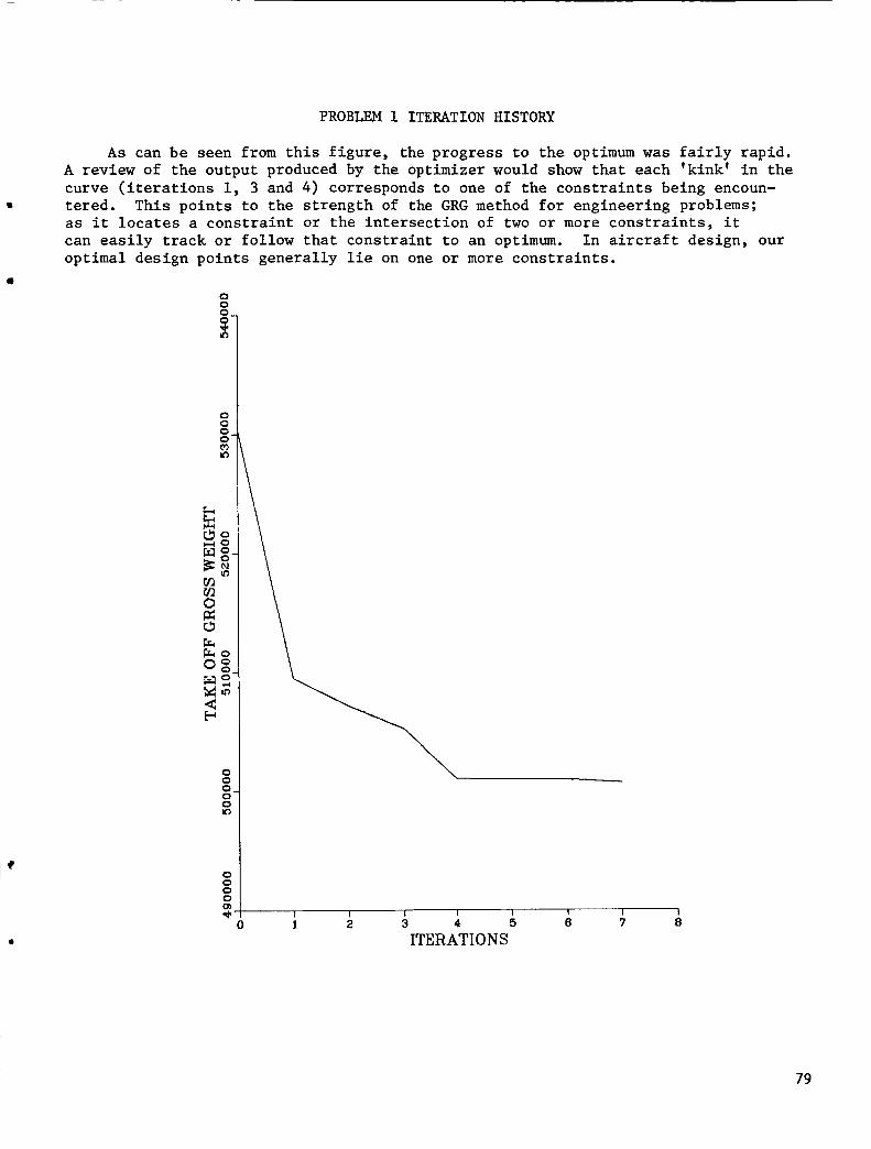
PROBLEM i ITERATION HISTORY

As can be seen from this figure, the progress to the optimum was fairly rapid.

A review of the output produced by the optimizer would show that each 'kink' in the

curve (iterations i, 3 and 4) corresponds to one of the constraints being encoun-

tered. This points to the strength of the GRG method for engineering problems;

as it locates a constraint or the intersection of two or more constraints, it

can easily track or follow that constraint to an optimum. In aircraft design, our

optimal design points generally lie on one or more constraints.

OOO_

00O.00

0o00

0

I I1 2

I I I

3 4 5

ITERATIONS

I I I6 7 8

79

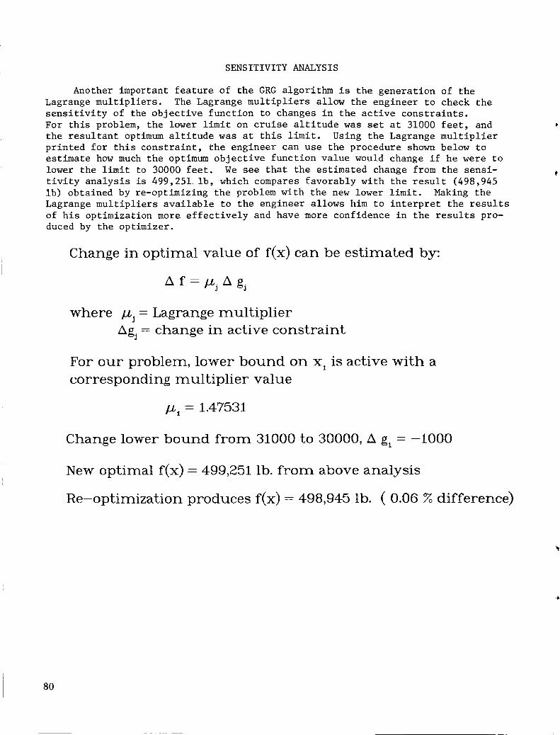
SENSITIVITY ANALYSIS

Another important feature of the GRG algorithm is the generation of the

Lagrange multipliers. The Lagrange multipliers allow the engineer to check the

sensitivity of the objective function to changes in the active constraints.

For this problem, the lower limit on cruise altitude was set at 31000 feet, and

the resultant optimum altitude was at this limit. Using the Lagrange multiplier

printed for this constraint, the engineer can use the procedure shown below to

estimate how much the optimum objective function value would change if he were to

lower the limit to 30000 feet. We see that the estimated change from the sensi-

tivity analysis is 499,251 Ib, which compares favorably with the result (498,945

Ib) obtained by re-optimizing the problem with the new lower limit. Making the

Lagrange multipliers available to the engineer allows him to interpret the results

of his optimization more effectively and have more confidence in the results pro-

duced by the optimizer.

Change in optimal value of f(x) can be estimated by:

A f = ttj A gj

where ttj = Lagrange multiplier

Ag_ = change in active constraint

For our problem, lower bound on x, is active with a

corresponding multiplier value

tz_ = 1.47531

Change lower bound from 31000 to 30000, A gl = --1000

New optimal f(x)= 499,251 lb. from above analysis

Re-optimization produces f(x) = 498,945 lb. ( 0.06 % difference)

80

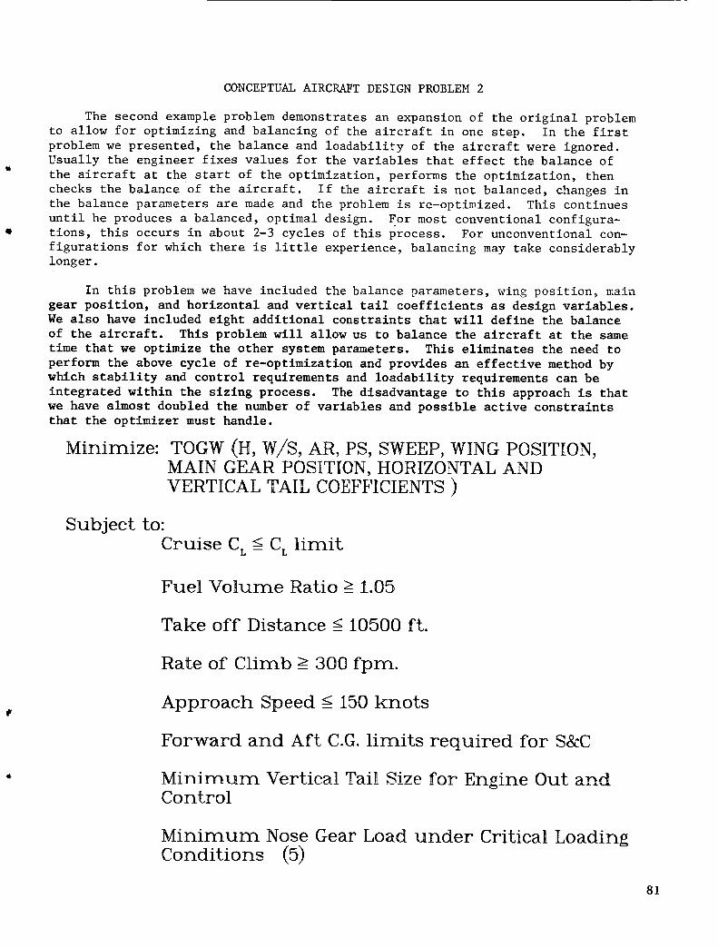
CONCEPTUAL AIRCRAFT DESIGN PROBLEM 2

The second example problem demonstrates an expansion of the original problem

to allow for optimizing and balancing of the aircraft in one step. In the first

problem we presented, the balance and loadability of the aircraft were ignored.

Usually the engineer fixes values for the variables that effect the balance of

the aircraft at the start of the optimization, performs the optimization, then

checks the balance of the aircraft. If the aircraft is not balanced, changes in

the balance parameters are made and the problem is re-optimized. This continues

until he produces a balanced, optimal design. For most conventional configura-

tions, this occurs in about 2-3 cycles of this process. For unconventional con-

figurations for which there is little experience, balancing may take considerably

longer.

In this problem we have included the balance parameters, wing position, main

gear position, and horizontal and vertical tail coefficients as design variables.

We also have included eight additional constraints that will define the balance

of the aircraft. This problem will allow us to balance the aircraft at the same

time that we optimize the other system parameters. This eliminates the need to

perform the above cycle of re-optimization and provides an effective method by

which stability and control requirements and loadability requirements can be

integrated within the sizing process. The disadvantage to this approach is that

we have almost doubled the number of variables and possible active constraints

that the optimizer must handle.

Minimize: TOGW (H, W/S, AR, PS, SWEEP, WING POSITION,MAIN GEAR POSITION, HORIZONTAL ANDVERTICAL TAIL COEFFICIENTS )

Subject to:

Cruise CL <- C L limit

Fuel Volume Ratio ___1.05

Take off Distance -< 10500 ft.

Rate of Climb _ 300 fpm.

Approach Speed __ 150 knots

Forward and Aft C.G. limits required for S&C

Minimum Vertical Tail Size for Engine Out andControl

Minimum Nose Gear Load under Critical LoadingConditions (5)

81

PROBLEM 2 RESULTS

The results for this larger problem are shown below. (The design concept is

different from the previous example, therefore comparison of weight is meaning-

less.) Again, this problem presents a challenge in variable and constraint

scaling for the optimizer that was handled in the same manner as for problem i.

As can be seen, the number of function evaluations is still low relative to

the size of the problem. The majority (117) of the evaluations were spent cal-

culating the numerical gradients.

In addition to the lower limit on altitude and the rate of climb specifica-

tion, the active constraints for this problem were the three stability and control

constraints (6, 7 and 8) on the tail sizes, and the minimum nose gear load under

one of the 5 critical loading conditions (constraint 13). This last constraint

contributes mostly to limiting the main gear location. This solution corresponds

to within .5% of a result obtained using the old method described earlier.

Start Pt Final Pt

H 32000 31000w/s 14o 54.tAR 6.5 7.6PS .9 .91SWEEP 30 25.5WING POS. .463 .479M.G. POS. .697 .652V .655 .524

H

V .090 .079v

TOGW 1,146,220 1,108,335

IterationsFunctions Eval.

Active Constraints:

13189

L

X 1 ,

constraints 4, 6, 7, 8, 13

82

PROBLEM 2 ITERATION HISTORY

The figure below illustrates that the method made good progress toward the

optimum and was close after about seven iterations. The problem terminated again

with the norm of the reduced gradient below the selected criterion. The elapsed

time for this problem was between 3-4 hours. The advantage here is that the

final optimal design Is also an aircraft that is acceptable with respect to sta-

bility and control and loadability requirements. This provides a valuable design

tool for those new concepts or configurations that prove difficult to balance.

OOO

0

0Q

0I ' I I l

1 2 3 4I I I I I I I I I I5 6 7 8 9 10 II 12 13 14

ITERATIONS

83

CONCLUSIONS

We have seen from these two examples that numerical optimization provides

substantial improvements in designer productivity over graphical techniques.

This allows the designer to investigate many more designs and concepts at a

very crucial time during the design process.

In our experience, the GRG algorithm provides a very reliable method for

conceptual aircraft optimization. The automated conceptual design system is used

on a daily basis at Lockheed in all conceptual design studies. The basic ability

of the method to easily locate optimum points that lie on constraint boundaries

appears to be well suited to this type of problem.

We have seen in the second design example that optimization can be used to

help solve design problems in which we have limited design experience. In fact,

we can now use optimization to formulate new design methods in areas in which it

is difficult to understand the interaction among design parameters and new tech-

nologies or concept. This is particularly true in conceptual aircraft design, inwhich innovation is more or less the rule.

The automated conceptual design system is used by engineers who are not opti-

mization experts. These engineers have been trained in how the optimizer works and

how to evaluate the results. But they often still require help in the development

of new formulations or in resolving whether the optimizer has truly reached a so-

lution. For these situations our experience suggests that someone with a strong

optimization background should 5e a member of any conceptual design study.

• Numerical optimization provides substantial improvementsin designer efficiency over manual techniques.

• The GRG method is a reliable method for conceptualaircraft optimization.

• Numerical optimization can help solve difficult design

problems where conventional wisdom is lacking.

• A team concept employing an optimization expert and

an experienced designer is essential.

84

le

u

e

e

e

e

REFERENCES

Abadie, J., and J. Carpenter, "The Generalization of the Wolfe Reduced Gradient

Method to the Case of Nonlinear Constraints," inOptimization (R. Fletcher,

Ed.), Academic Press, New York, 1969.

Lasdon, L. S., A. D. Waren, A. Jain, and M. Ratner, "Design and Testing of a

Generalized Reduced Gradient Code for Nonlinear Programming," ACM Trans.

Math. Software, Vol. 4, No. i, pp. 34-50, 1978.

Gahriele, G. A. and K. M. Ragsdell, "The Generalized Reduced Gradient Method:

A Reliable Tool for Optimal Design," ASME J. Eng. Ind., Vol. 99, No. 2,

pp. 384-400, May 1977.

Broyden, C. G., "A Class of Methods for Solving Nonlinear Simultaneous Equations, !'

Math. Comp., V01. 21, pp. 368-381, 1965.

Gabrlele, G. A. and K. M. Ragsdell, "OPT: A Nonlinear Programming Code in

Fortran IV - User's Manual," Purdue Research Foundation, West Lafayette, IN,

Jan. 1976.

Root, R. R., and K. M. Ragsdell, "Computational Enhancements of the Method of

Multipliers," ASME J. Mech. Des., Vol. 102, pp. 517-523, 1970.

85