arX

iv:n

lin/0

3020

59v4

[nl

in.S

I] 2

Feb

200

4

1

Progress of Theoretical Physics, 2004

N -Soliton Collision in the Manakov Model

Takayuki Tsuchida∗)

Graduate School of Mathematical Sciences, University of Tokyo,

Tokyo 153-8914, Japan

(Received March 14, 2003)

We investigate soliton collisions in the Manakov model, which is a system of couplednonlinear Schrodinger equations that is integrable via the inverse scattering method. Com-puting the asymptotic forms of the general N-soliton solution in the limits t → ∓∞, weelucidate a mechanism that factorizes an N-soliton collision into a nonlinear superpositionof(N

2

)pair collisions with arbitrary order. This removes the misunderstanding that multi-

particle effects exist in the Manakov model and provides a new “set-theoretical” solutionto the quantum Yang-Baxter equation. As a by-product, we also obtain a new nontrivialrelation among determinants and extended determinants.

§1. Introduction

In recent years, there has been a surge of interest in some systems of coupled nonlinearSchrodinger (coupled NLS) equations because of their relevance in nonlinear optics.1), 2), 3) Amongsuch systems, this paper focuses on the following system of coupled NLS equations:

iqt + qxx + 2||q||2q = 0, q = (q1, q2, · · · , qm). (1.1)

Here ||q||2 ≡ q · q† =∑m

j=1 |qj |2, where the superscript † denotes Hermitian conjugation. The

subscripts t and x denote the partial differentiation with respect to these variables. It is wellknown that (1.1) is a completely integrable system.4), 5) We call (1.1) the Manakov model, sincethe two-component (m = 2) case of (1.1) was solved for the first time by Manakov4) using theinverse scattering method (ISM). The extension of the ISM to the general m-component case isstraightforward.5) Nevertheless, the value of m is extremely important when we consider solitonsolutions. Them = 2 case is merely a special case of the general m case. The most interesting is thecase in which the total number of solitons, say N , is equal to the number of components, m. Indeed,in the N = m case, the coefficient vectors for the hyperbolic-secant-type envelope of solitons [see,e.g., u1 in (2.12)], which we refer to after normalization as polarization vectors, are just sufficientto span the vector space C

m, in which q exists. Soliton solutions in the other cases (N > m orN < m) are obtained from those in this case through a special choice of soliton parameters or theoperation of a unitary transformation. In this paper, we consider the most general case, in whichN and m are arbitrary positive integers. Then, the most interesting case, N = m, is automaticallyincluded.

Although the integrability of the Manakov model (1.1) has been established formally throughapplication of the ISM, multi-soliton dynamics in the model remain to be clarified. There are two

∗) E-mail: tsuchida@poisson.ms.u-tokyo.ac.jp

typeset using PTPTEX.cls 〈Ver.0.89〉

2

reasons for this. One reason is that the vector nature of (1.1), which supports the internal degreesof freedom of solitons, leads to complicated behavior. Indeed, even a two-soliton collision is highlynontrivial,6), 7), 8), 9) as not only does a displacement of the soliton centers depend on the initialpolarization vectors but also the polarization vectors themselves are changed. Therefore, in thismodel, the effect of an N -soliton collision can never be written as the algebraic sum of the effectsof pair collisions (at least, if we employ only the initial soliton parameters). This is quite differentfrom the NLS case [i.e. (1.1) with m = 1], in which the effect of an N -soliton collision in fact can bewritten as the algebraic sum of the effects of pair collisions (in which the order of the pair collisionsdoes not matter).10), 11), 12) The other reason is that Manakov gave a rather misleading descriptionof an N -soliton collision in Ref. 4). We quote the corresponding part, the first two sentences of thelast paragraph of §2 in Ref. 4):

Comparison of relations (17) and (18) indicates that an N -soliton collision does not,in general, reduce to a pair collision. This is clear, for example, from the fact that theexpression for S+

k contains S+j with j > k, which depend on the initial parameters

of all the remaining solitons.

(♣)

The relations (17) referred to here are given by

S+N =

{∏

n<N

α −111 (ζN , ζn)

}

αT (ζN , ζ1,S−1 ) . . . α

T (ζN , ζN−1,S−N−1)S

−N ,

S+i =

{∏

k>i

α11(ζi, ζk)

}{∏

n<i

α −111 (ζi, ζn)

}

α∗(ζ∗i , ζi+1,S+i+1) . . . α

∗(ζ∗i , ζN ,S+N )

· αT (ζi, ζ1,S−1 ) . . . α

T (ζi, ζi−1,S−i−1)S

−i , i = 1, 2, · · · , N − 1,

while the relations (18) are given by

S+2 = α −1

11 (ζ2, ζ1) αT (ζ2, ζ1,S

−1 )S

−2 ,

S+1 = α11(ζ1, ζ2) α

∗(ζ∗1 , ζ2,S+2 )S

−1 .

We now briefly explain the situation considered and the notation used in Ref. 4). The equations(17) of Ref. 4) represent the solution for the collision of N solitons (to which we refer as solitons-1,2, · · · , N), while the equations (18) represent that for two solitons. We note that the equations(18) are obtained from (17) by setting N = 2. The equations (17) were derived through analysisbased on and intuition gained from the ISM. It is assumed that a soliton designated by a largernumber moves faster along the x-axis. That is, soliton-i overtakes∗) solitons-1, 2, · · · , i− 1 and isovertaken by solitons-i+1, i+2, · · · , N as time t passes from −∞ to +∞. The velocity of soliton-iand its amplitude are determined by the complex parameter ζi, which is time independent. Thequantities Si are column vectors with two complex components, corresponding to the choice of

m = 2 in Ref. 4). The vector norm ||Si||[= (S†

i · Si)12

]determines the center position of soliton-i,

while the normalized vector Si/||Si|| gives its polarization vector after the operation of Hermitian∗) Throughout this paper, we use the term “overtake” if only the relative velocity is positive. Thus it can be used

for head-on collisions, etc.

3

conjugation. The superscripts + and − denote the final state (t → +∞) and the initial state(t → −∞), respectively. α11 is a scalar function and α is a 2 × 2 matrix function. We do not givetheir explicit forms, which are not important in the following discussion. The superscripts T and∗ denote the operations of transposition and complex conjugation, respectively.

Although the assertion (♣) is somewhat ambiguous, the most natural and reasonable interpre-tation seems to be the following:

Let us try to explain (17) by assuming that the N solitons collide pairwise in ac-cordance with (18). Then, the first equation in (17) can be understood as follows.Soliton-N first overtakes soliton-N − 1 in its initial state, i.e. soliton-N − 1, whichhas not collided with other solitons. Next, soliton-N overtakes soliton-N − 2, whichhas not collided with other solitons. . . . Finally, it overtakes soliton-1, which has notcollided with other solitons.

Similarly, the second equation in (17) can be understood as follows. Soliton-iovertakes solitons-i − 1, i − 2, · · · , 1 in this order, none of which has collided withother solitons. Next, soliton-i is overtaken by solitons-N , N − 1, · · · , i + 1 in theirfinal states, i.e. those which will not collide with other solitons.

If we attempt to diagram these events, we immediately encounter a contradiction.This indicates that an N -soliton collision cannot be described as a sequence of paircollisions, since the matrices α for different sets of arguments do not commute ingeneral.

The logic of the above interpretation is not mathematically rigorous, but it seems to be correctif the complex structure of (17) is taken into account. It might also be possible to interpret theassertion (♣) in a different way. In any case, it appears that an N -soliton collision in the Manakovmodel (1.1) does not reduce to a pair collision, and thus that some multi-particle effects exist inthe Manakov model. However, in fact this is not true.

The main goal of this paper is to clear up this misunderstanding. We explicitly demonstratea mechanism that factorizes an N -soliton collision in the Manakov model (1.1) into a nonlinear

superposition of pair collisions. Here, we have used the term “nonlinear” to express the factthat the considered superposition is no longer additive. For the sake of definiteness, we explainin advance what we prove in terms of the Manakov notation, which also gives the definition offactorization in this paper. We first interpret the equations (18) as forming a nonlinear mappingwith two complex parameters, f(ζ2, ζ1), which maps the initial state {S−

2 ,S−1 } into the final state

{S+2 ,S

+1 }. Then, we can use the mapping f(ζj, ζk) to evaluate in an N -soliton collision the effect

of the two-soliton collision whereby soliton-j in a state Sj overtakes soliton-k in a state Sk. For a

given order of(N2

)pair collisions, we consider the corresponding composition of the

(N2

)mappings:

f(ζj, ζk), N ≥ j > k ≥ 1. Then, regardless of the order of the pair collisions,∗) the composedmapping maps the initial state {S−

N ,S−N−1, · · · ,S

−1 } exactly to the final state {S+

N ,S+N−1, · · · ,S

+1 }

given by the equations (17).To prove this factorization, we do not employ the Manakov results, equations (17) and (18), for

∗) Here, we are referring to the order in which neighboring solitons collide pairwise. That is, unlike the m = 1

case (scalar NLS), we do not consider virtual collisions between non-neighboring solitons.

4

the following two reasons. One reason is that, although it is ingenious and seems to be correct, thederivation of (17) in Ref. 4) is neither very rigorous nor understandable to the reader not familiarwith the ISM. The other reason is that the equations (17) are not tractable for our purpose. In thispaper, we employ a more straightforward approach to obtain another formula for the asymptoticbehavior of N solitons. We start from an explicit formula for the N -soliton solution of the matrixNLS equation derived using the ISM in Ref. 13). Through a simple reduction, we obtain an explicitformula for the general N -soliton solution of the Manakov model (1.1).14) To make the paperself-contained, we first set N = 2 and compute the asymptotic forms of the two-soliton solutionin the t → ∓∞ limits in our notation. These solutions define the collision laws of two solitons inthe Manakov model, which are essentially the same as those given by the equations (18). Next,we consider the general N case and compute the asymptotic forms of the N -soliton solution in thet → ∓∞ limits. To express the polarization vectors appearing in the asymptotic forms concisely,we extend the definition of a determinant in such a way that the last column of an extendeddeterminant consists of vectors. This determinant represents a vector defined in terms of theLaplace expansion with respect to the last column. We find a beautiful relation which casts theHermitian product between such extended determinants into the form of a product of conventionaldeterminants. Using this relation and the Jacobi formula for determinants, we prove that an N -soliton collision in the Manakov model (1.1) can be factorized into a nonlinear superposition of(N2

)pair collisions in arbitrary order. This reveals∗) the following two properties of the Manakov

model:

(a) An N -soliton collision is composed of a nonlinear superposition of(N2

)pair collisions of certain

order.

(b) The composition of(N2

)mappings corresponding to pair collisions in an N -soliton collision

yields the same mapping for every possible order of composition.

We remark that solitons are not mass points, and do not have compact support. Rather, theyare structures with infinitely long tails. Even in a two-soliton collision, it takes an infinite timefor the solitons to completely recover their own shapes. Taking this into consideration, it is moremeaningful to understand this factorization conceptually than phenomenologically. It is unlikelythat properties (a) and (b) are related directly. We note that proving (a) is equally difficult forevery order of pair collisions and that proving (b) for arbitrary N reduces to proving it for N = 3,that is, the following:

(b’) The composition of three mappings corresponding to pair collisions in a three-soliton collisiondoes not depend on the (conceptional) order of pair collisions.

The property (b’) is called the Yang-Baxter property. The validity of this property means that thecollision laws of two solitons in the Manakov model (1.1) give a “set-theoretical” solution to thequantum Yang-Baxter equation.15) To the best of the author’s knowledge, this solution is new. Wemention that another “set-theoretical” solution to the quantum Yang-Baxter equation is studiedby Veselov16) through investigation of the matrix KdV equation.

A few interesting ideas17), 18), 19) have been proposed to explain in a general manner the pairwise

∗) To deduce property (b) from the factorization rigorously in the present setting, some discussion is needed.

This is given in §5.

5

nature of soliton collisions in integrable systems. However, those ideas seem to be too intuitive intheir present forms to complete a mathematically rigorous proof. For instance, it is not obviousthat a pair collision is unaffected by the other solitons given only that they are far away, or thatthe final result is invariant when the order of multiple limits is changed. In addition, unlike thiswork, those works do not elucidate a nice mechanism of factorization.

Finally, we would like to comment on the literature concerning the Manakov model (1.1). Multi-soliton solutions of the Manakov model have already been obtained using the Hirota method20), 21), 22)

(see also Refs. 23) and 24) for results obtained with another method). In this sense, although itis very useful, the explicit formula for the N -soliton solution obtained in this paper may not beessentially new.∗) The main contribution of this work is the elucidation of the pairwise nature ofsoliton collisions in the Manakov model. The results of this paper were obtained by the author inthe summer of 2000 and presented at the autumn meeting of the Physical Society of Japan in thatyear. Very recently, he encountered some papers25), 26), 27)∗∗) which pose the same problem (butdo not solve it completely). In particular, in Ref. 27), which actually appeared after the first sub-mission of this paper, Kanna and Lakshmanan gave a “proof” of the pairwise collision nature of athree-soliton collision. Unfortunately, the “proof” of Kanna-Lakshmanan27) is absolutely incorrect.Indeed, in addition to a few fatal mistakes, their “proof” as a whole is a typical example of circularreasoning.

The remainder of this paper is organized as follows. In §2, we derive an explicit formula forthe N -soliton solution of the Manakov model.14) In §3, we obtain the collision laws of two solitons.In §4, we compute the asymptotic forms of the N -soliton solution in the limits t → ∓∞. In §5, weelucidate a mechanism that factorizes an N -soliton collision into a nonlinear superposition of paircollisions and discuss the Yang-Baxter property. Section 6 is devoted to concluding remarks.

§2. Explicit formula for the general N-soliton solution

In this section, considering a reduction of a formula given in Ref. 13), we derive an explicitformula for the general N -soliton solution of the Manakov model (1.1).

In Ref. 13), under vanishing boundary conditions, we applied the ISM to nonlinear evolutionequations associated with the generalized Zakharov-Shabat eigenvalue problem:

[Ψ1

Ψ2

]

x

=

[−iζI Q−Q† iζI

] [Ψ1

Ψ2

]

. (2.1)

Here, ζ is the spectral parameter, I is the m×m unit matrix, and Q is an m ×m matrix-valuedpotential function. The first two of the nonlinear evolution equations associated with (2.1) are thematrix NLS equation,

iQt +Qxx + 2QQ†Q = O, (2.2)

and the matrix complex mKdV equation,

Qt +Qxxx + 3(QxQ†Q+QQ†Qx) = O. (2.3)

∗) In any case, our formula has the advantage of compactness in its own right.∗∗) Actually, the work of Park and Shin25) is very similar to that of Steudel.28)

6

We mention that integrable space-discretizations of (2.2) and (2.3) were found recently29) (see alsothe relevant work in Refs. 22) and 30),31),32)). The general N -soliton solution of (2.2) or (2.3) isexpressed as13)

Q(x, t) = −2i( I I · · · I︸ ︷︷ ︸

N

) S−1

C1(t)† e−2iζ∗1x

C2(t)† e−2iζ∗2x

...CN (t)† e−2iζ∗Nx

, (2.4)

where the mN ×mN matrix S is given by

Sjk = δjkI −N∑

l=1

e2i(ζl−ζ∗j )x

(ζl − ζ∗k)(ζl − ζ∗j )Cj(t)

†Cl(t), 1 ≤ j, k ≤ N. (2.5)

Here, ζj are discrete eigenvalues in the upper-half plane of ζ (Im ζj > 0), each of which determinesa bound state in the potential Q. The quantities Cj(t) are m × m nonzero matrices whose timedependences are given by

Cj(t) = Cj(0)e4iζ2j t, j = 1, 2, · · · , N, (2.6)

for the matrix NLS equation (2.2), and

Cj(t) = Cj(0)e8iζ3j t, j = 1, 2, · · · , N,

for the matrix complex mKdV equation (2.3), respectively.Let us consider a reduction of the N -soliton solution of the matrix NLS equation to that of the

Manakov model. We restrict the matrix Q to the form

Q =

q1 q2 · · · qm0 0 · · · 0...

.... . .

...0 0 · · · 0

≡

[q

O

]

, (2.7)

so that the matrix NLS equation (2.2) is reduced to the Manakov model (1.1). In this case, thematrices Cj(t)

† must have the same form as Q, from their definition,13), 14)

Cj(t)† =

c(1)j c

(2)j · · · c

(m)j

0 0 · · · 0...

.... . .

...0 0 · · · 0

≡ i

[cj(t)O

]

, j = 1, 2, · · · , N. (2.8)

Conversely, if Cj(t)† take the form (2.8), Q(x, t) given by the formula (2.4) with (2.5) fits the form

(2.7). Then, the formula can be compressed into a compact form,14)

q(x, t) = 2N∑

j=1

N∑

k=1

(T−1)jke−2iζ∗

kxck(t),

7

where the N ×N matrix T is given by

Tjk = δjk −

N∑

l=1

e2i(ζl−ζ∗j )x

(ζl − ζ∗k)(ζl − ζ∗j )cj(t) · cl(t)

†, 1 ≤ j, k ≤ N.

Thanks to (2.6) and (2.8), the time dependence of cj(t) is given by

cj(t) = e−4iζ∗2j tcj(0), j = 1, 2, · · · , N.

The above set of equations gives a formula for the general N -soliton solution of the Manakov model(1.1) under vanishing boundary conditions. Let us rewrite this into a form convenient to investigatethe asymptotic behavior. We first rewrite it as

q(x, t) = 2

N∑

j=1

N∑

k=1

(W−1)jke−i[(ζk+ζ∗

k)x+2(ζ2

k+ζ∗2

k)t]ck(0),

where the N ×N matrix W is given by

Wjk = δjke−i[(ζj−ζ∗j )x+2(ζ2j −ζ∗2j )t] −

N∑

l=1

cj(0) · cl(0)†

(ζl − ζ∗k)(ζl − ζ∗j )ei[(ζl−ζ∗

l)x+2(ζ2

l−ζ∗2

l)t]

× ei[(ζl+ζ∗l)x+2(ζ2

l+ζ∗2

l)t]e−i[(ζj+ζ∗j )x+2(ζ2j +ζ∗2j )t], 1 ≤ j, k ≤ N.

Next, we introduce the parametrization

ζj = ξj + iηj (ξj ∈ R, ηj > 0),

cj(0) = 2ηje−αjuj (αj ∈ R, ||uj || = 1),

and employ the following abbreviations:

τj ≡ −i[(ζj − ζ∗j )x+ 2(ζ2j − ζ∗2j )t] = 2ηj(x+ 4ξjt),

Θj ≡ (ζj + ζ∗j )x+ 2(ζ2j + ζ∗2j )t = 2ξjx+ 4(ξ2j − η2j )t.

In this way, we obtain the simplest formula for the general N -soliton solution of the Manakov model(1.1),

q(x, t) = 2N∑

j=1

N∑

k=1

(U−1)jke−iΘkuk, (2.9)

where the N ×N matrix U is given by

Ujk =eτj+αj

2ηjδjk +

N∑

l=1

λjkle−(τl+αl)+i(Θl−Θj), 1 ≤ j, k ≤ N, (2.10)

with

λjkl = −2ηl(uj · u

†l )

(ζl − ζ∗k)(ζl − ζ∗j ). (2.11)

8

If we set N = 1 in the above formula, we obtain the one-soliton solution,

q(x, t) = 2η1 sech(τ1 + α1)e−iΘ1u1. (2.12)

Therefore, we understand the significance of each parameter/coordinate as follows:

2ηj : amplitude of soliton-j,

−4ξj : velocity of soliton-j’s envelope,

τj : coordinate for observing soliton-j’s envelope,

Θj : coordinate for observing soliton-j’s carrier waves,

uj : polarization vector of soliton-j (||uj|| = 1).

To be precise, in the case of two or more solitons, the real polarization vectors are not invariantand change under soliton collision. The vector uj defines the bare polarization of soliton-j, which isrealized when it becomes the rightmost soliton. This point is demonstrated below. In the following,we assume that all the soliton velocities are distinct, so that every soliton collides with all others.

§3. Two-soliton collision

In this section, we compute the asymptotic forms of the two-soliton solution in the limitst → ∓∞, which define the collision laws of two solitons in the Manakov model (1.1).

We first write out the two-soliton solution given by (2.9) with N = 2. According to (2.10), thematrix U in this case takes the form

U =

eτ1+α1

2η1+

2∑

l=1

λ11le−(τl+αl)+i(Θl−Θ1)

2∑

l=1

λ12le−(τl+αl)+i(Θl−Θ1)

2∑

l=1

λ21le−(τl+αl)+i(Θl−Θ2) eτ2+α2

2η2+

2∑

l=1

λ22le−(τl+αl)+i(Θl−Θ2)

.

Then, the two-soliton solution is given by

q(x, t) =2

detU

{[

eτ2+α2

2η2+

2∑

l=1

λ22le−(τl+αl)+i(Θl−Θ2) −

2∑

l=1

λ21le−(τl+αl)+i(Θl−Θ2)

]

e−iΘ1u1

+

[

eτ1+α1

2η1+

2∑

l=1

λ11le−(τl+αl)+i(Θl−Θ1) −

2∑

l=1

λ12le−(τl+αl)+i(Θl−Θ1)

]

e−iΘ2u2

}

, (3.1)

with

detU =eτ1+α1

2η1

eτ2+α2

2η2+

eτ1+α1

2η1

2∑

l=1

λ22le−(τl+αl)+i(Θl−Θ2) +

eτ2+α2

2η2

2∑

l=1

λ11le−(τl+αl)+i(Θl−Θ1)

+ e−(τ1+α1)e−(τ2+α2)∑

{l1,l2}={1,2}

∣∣∣∣

λ11l1 λ12l1

λ21l2 λ22l2

∣∣∣∣. (3.2)

9

Here, we have simplified the expression of detU using the relations∣∣∣∣

λ11l λ12l

λ21l λ22l

∣∣∣∣= 0, l = 1, 2, (3.3)

which can be proved straightforwardly.Next, we assume that

ξ1(= Re ζ1) > ξ2(= Re ζ2)

and investigate the asymptotic behavior of q(x, t) as t → ∓∞. This is accomplished by identifyingthe dominant terms in the numerator of (3.1) and its denominator (3.2). We here note the relationτ1/η1 = τ2/η2 + 8(ξ1 − ξ2)t.

In the limit t → −∞, we haveτ1η1

≪τ2η2

.

In this case, we have to consider separately the two regions (1−) and (2−) defined below. It iseasily seen that q ≃ 0 in all other regions.(1−) finite τ1, τ2 → +∞

In this case, the dominant terms are those which contain the factor eτ2 . Then, using therelation λ111 = 1/(2η1), we obtain

q ≃2 eτ2+α2

2η2e−iΘ1u1

eτ1+α1

2η1eτ2+α2

2η2+ eτ2+α2

2η2λ111e−(τ1+α1)

= 2η1 sech(τ1 + α1)e−iΘ1u1. (3.4)

(2−) τ1 → −∞, finite τ2Here, the dominant terms are those which contain the factor e−τ1 . Then, we obtain

q ≃2[(λ221 − λ211)e

−(τ1+α1)e−iΘ2u1 + (λ111 − λ121)e−(τ1+α1)e−iΘ2u2

]

eτ2+α2

2η2λ111e−(τ1+α1) + e−(τ1+α1)e−(τ2+α2)

∑

{l1,l2}={1,2}

∣∣∣∣

λ11l1 λ12l1

λ21l2 λ22l2

∣∣∣∣

. (3.5)

In terms of φ12 defined by

e−2φ12 ≡1

λ111λ222

∑

{l1,l2}={1,2}

∣∣∣∣

λ11l1 λ12l1

λ21l2 λ22l2

∣∣∣∣, (3.6)

we can rewrite the asymptotic form (3.5) as

q ≃ 2η2 sech(τ2 + α2 + φ12)e−iΘ2 × eφ12

[(λ221 − λ211

λ111

)

u1 +

(

1−λ121

λ111

)

u2

]

. (3.7)

Here, φ12 is always taken as real, since (3.6) can be rewritten as [cf. (3.3) and (2.11)]

e−2φ12 =1

λ111λ222

∣∣∣∣

λ111 + λ112 λ121 + λ122

λ211 + λ212 λ221 + λ222

∣∣∣∣

10

= (2η1)(2η2)

∣∣∣∣∣∣

iu1·u

†1

ζ1−ζ∗1iu1·u

†2

ζ2−ζ∗1

iu2·u

†1

ζ1−ζ∗2iu2·u

†2

ζ2−ζ∗2

∣∣∣∣∣∣

∣∣∣∣∣

i 2η1ζ1−ζ∗1

i 2η1ζ1−ζ∗2

i 2η2ζ2−ζ∗1

i 2η2ζ2−ζ∗2

∣∣∣∣∣

=

∣∣∣∣

ζ1 − ζ2ζ1 − ζ∗2

∣∣∣∣

2{

1 +(ζ1 − ζ∗1 )(ζ2 − ζ∗2 )

|ζ1 − ζ∗2 |2

∣∣∣u1 · u

†2

∣∣∣

2}

(> 0).

In the limit t → +∞, we haveτ1η1

≫τ2η2

.

In this case, we have to consider separately the two regions (2+) and (1+) defined below. It iseasily seen that q ≃ 0 in all other regions.(2+) τ1 → +∞, finite τ2

In this case, the dominant terms are those which contain the factor eτ1 . Then, using therelation λ222 = 1/(2η2), we obtain

q ≃2 eτ1+α1

2η1e−iΘ2u2

eτ1+α1

2η1eτ2+α2

2η2+ eτ1+α1

2η1λ222e−(τ2+α2)

= 2η2 sech(τ2 + α2)e−iΘ2u2. (3.8)

(1+) finite τ1, τ2 → −∞In this case, the dominant terms are those which contain the factor e−τ2 . Then, with the helpof (3.6), we obtain

q ≃2[(λ222 − λ212)e

−(τ2+α2)e−iΘ1u1 + (λ112 − λ122)e−(τ2+α2)e−iΘ1u2

]

eτ1+α1

2η1λ222e−(τ2+α2) + e−(τ1+α1)e−(τ2+α2)

∑

{l1,l2}={1,2}

∣∣∣∣

λ11l1 λ12l1

λ21l2 λ22l2

∣∣∣∣

= 2η1 sech(τ1 + α1 + φ12)e−iΘ1 × eφ12

[(

1−λ212

λ222

)

u1 +

(λ112 − λ122

λ222

)

u2

]

. (3.9)

Taking the sum of (3.4) and (3.7), or (3.8) and (3.9), with a slight simplification, we arrive at thefollowing theorem.

Theorem 3.1. The asymptotic forms of the two-soliton solution of the Manakov model (1.1) are

as follows (see also Fig. 1):as t → −∞,

q ≃ 2η1 sech(τ1 + α1)e−iΘ1u1 + 2η2 sech(τ2 + α2 + φ12)e

−iΘ2u{1},2;

as t → +∞,

q ≃ 2η1 sech(τ1 + α1 + φ12)e−iΘ1u{2},1 + 2η2 sech(τ2 + α2)e

−iΘ2u2.

Here φ12 and u{1},2, u{2},1 are given by

e−2φ12 =

∣∣∣∣

ζ1 − ζ2ζ1 − ζ∗2

∣∣∣∣

2{

1 +(ζ1 − ζ∗1 )(ζ2 − ζ∗2 )

|ζ1 − ζ∗2 |2

∣∣∣u1 · u

†2

∣∣∣

2}

,

11

and

u{1},2 = eφ12ζ∗1 − ζ∗2ζ1 − ζ∗2

{

u2 −ζ1 − ζ∗1ζ1 − ζ∗2

(

u2 · u†1

)

u1

}

,

u{2},1 = eφ12ζ∗2 − ζ∗1ζ2 − ζ∗1

{

u1 −ζ2 − ζ∗2ζ2 − ζ∗1

(

u1 · u†2

)

u2

}

.

Theorem 3.1 defines the collision laws of two solitons in the Manakov model, which we use in §5to factorize an N -soliton collision into pair collisions. Here, we mention some important propertiesof the collision laws:

• A two-soliton collision changes neither the amplitudes of the solitons nor the modulus of theHermitian product of the polarization vectors. In fact, recalling that ||u1|| = ||u2|| = 1, we canprove by direct computations that

∣∣∣∣u{1},2

∣∣∣∣ =

∣∣∣∣u{2},1

∣∣∣∣ = 1,

∣∣∣u1 · u

†{1},2

∣∣∣ =

∣∣∣u{2},1 · u

†2

∣∣∣ ,

∣∣∣u1 · u

†2

∣∣∣ =

∣∣∣u{2},1 · u

†{1},2

∣∣∣ .

Although we omit here the tiresome proof, the most important relation∣∣∣∣u{1},2

∣∣∣∣ =

∣∣∣∣u{2},1

∣∣∣∣ = 1

is shown in §5 in a more general context. This relation shows that the collision is elastic if weobserve it with conserved density, ||q||2 =

∑mj=1 |qj |

2.• As a result of the collision, the polarization vectors rotate nontrivially on the unit sphere in

Cm. Thus, if we observe the collision with respect to each component qk, it appears as if it

were inelastic.• We have expressed φ12, u{1},2 and u{2},1 in terms of u1 and u2. Then, the collision laws are

symmetric with respect to interchange of the subscripts 1 and 2. This form of the collisionlaws is very useful in studying the factorization of an N -soliton collision into pair collisions.For any fixed unit vector u1, we can invert the mapping u2 7→ u{1},2 using the following

relation for the projection operator u†1u1 (cf. (u†

1u1)2 = u

†1u1):

(

I −ζ1 − ζ∗1ζ1 − ζ∗2

u†1u1

)(

I +ζ1 − ζ∗1ζ∗1 − ζ∗2

u†1u1

)

= I.

Then, we can express φ12, u2 and u{2},1 in terms of u1 and u{1},2 as Manakov did in Ref. 4):

e−2φ12 =

∣∣∣∣

ζ1 − ζ2ζ1 − ζ∗2

∣∣∣∣

2{

1−(ζ1 − ζ∗1 )(ζ2 − ζ∗2 )

|ζ1 − ζ2|2

∣∣∣u1 · u

†{1},2

∣∣∣

2}−1

, (3.10a)

u2 = e−φ12ζ1 − ζ∗2ζ∗1 − ζ∗2

{

u{1},2 +ζ1 − ζ∗1ζ∗1 − ζ∗2

(

u{1},2 · u†1

)

u1

}

, (3.10b)

u{2},1 = e−φ12ζ∗2 − ζ1ζ2 − ζ1

{

u1 −ζ2 − ζ∗2ζ2 − ζ1

(

u1 · u†{1},2

)

u{1},2

}

. (3.10c)

Owing to the lack of symmetry under the exchange of 1 and 2 (even after a change of thevector notation), this new form of the collision laws is not useful in studying the factorization

12

problem. On the other hand, it is of prime importance in explicitly showing that a two-solitoncollision can be expressed as a mapping from the initial state to the final state. Moreover,using (3.10), we can easily check that if ||u1|| =

∣∣∣∣u{1},2

∣∣∣∣ = 1, then ||u2|| = 1. This verifies that

for any unit vector u1, the mapping u2 7→ u{1},2 in Theorem 3.1 is a bijection on the unitsphere. We use this fact in §5 to prove the Yang-Baxter property of the mapping (3.10).

13

soliton-1

soliton-1 soliton-2

soliton-2

interactionranget

q ≃ 2η2 sech(τ2 + α2 + φ12)e−iΘ2u{1},2 q ≃ 2η1 sech(τ1 + α1)e

−iΘ1u1

q ≃ 2η1 sech(τ1 + α1 + φ12)e−iΘ1u{2},1 q ≃ 2η2 sech(τ2 + α2)e

−iΘ2u2

Fig. 1. Two-soliton collision.

14

§4. Asymptotic behavior of the N-soliton solution

In this section, we compute the asymptotic forms of theN -soliton solution in the limits t → ∓∞and simplify them as much as possible. Extensions of some techniques applied to the KdV equationare used.33), 34), 35)

We first rewrite the N -soliton solution (2.9) before considering the limits t → ∓∞. We use thetilde to denote cofactors. For instance, the cofactor Ukj is obtained by deleting the k-th row andthe j-th column from the determinant of U and multiplying it by (−1)k+j. Using the definition ofU given in (2.10) and the multilinearity of determinants, we can rewrite (2.9) as

q(x, t)

=2

detU

N∑

j=1

N∑

k=1

Ukje−iΘkuk

=2

detU

[

(U11 + · · ·+ U1N )e−iΘ1u1 + · · ·+ (UN1 + · · · + UNN )e−iΘNuN

]

=2

detU

∣∣∣∣∣∣∣∣∣

1 1 · · · 1U21 U22 · · · U2N...

.... . .

...UN1 UN2 · · · UNN

∣∣∣∣∣∣∣∣∣

e−iΘ1u1 + · · ·+

∣∣∣∣∣∣∣∣∣

U11 U12 · · · U1N...

......

UN−11 UN−12 · · · UN−1N

1 1 · · · 1

∣∣∣∣∣∣∣∣∣

e−iΘNuN

=2

detU

N−1∑

n=0

∑

2≤j1<···<jn≤N

N∏

k=2k 6=j1,··· ,jn

eτk+αk

2ηk

N∑

l1,··· ,ln=1

e−(τl1+αl1)+i(Θl1

−Θj1)

× · · · × e−(τln+αln )+i(Θln−Θjn )

∣∣∣∣∣∣∣∣∣

1 1 · · · 1λj11l1 λj1j1l1 · · · λj1jnl1

......

. . ....

λjn1ln λjnj1ln · · · λjnjnln

∣∣∣∣∣∣∣∣∣

e−iΘ1u1

+ · · ·+N−1∑

n=0

∑

1≤j1<···<jn≤N−1

N−1∏

k=1k 6=j1,··· ,jn

eτk+αk

2ηk

N∑

l1,··· ,ln=1

e−(τl1+αl1)+i(Θl1

−Θj1)

× · · · × e−(τln+αln )+i(Θln−Θjn )

∣∣∣∣∣∣∣∣∣

λj1j1l1 · · · λj1jnl1 λj1Nl1...

. . ....

...λjnj1ln · · · λjnjnln λjnNln

1 · · · 1 1

∣∣∣∣∣∣∣∣∣

e−iΘNuN

. (4.1)

Similarly, we can rewrite the determinant of U as

detU

15

=

N∏

k=1

eτk+αk

2ηk+

N∑

j1=1

N∏

k=1k 6=j1

eτk+αk

2ηk

N∑

l1=1

e−(τl1+αl1)+i(Θl1

−Θj1)λj1j1l1

+∑

1≤j1<j2≤N

N∏

k=1k 6=j1,j2

eτk+αk

2ηk

N∑

l1,l2=1

e−(τl1+αl1)+i(Θl1

−Θj1)e−(τl2+αl2

)+i(Θl2−Θj2

)

∣∣∣∣

λj1j1l1 λj1j2l1

λj2j1l2 λj2j2l2

∣∣∣∣

+ · · ·+

N∑

l1,··· ,lN=1

e−(τl1+αl1)+i(Θl1

−Θ1) · · · e−(τlN +αlN)+i(ΘlN

−ΘN )

∣∣∣∣∣∣∣

λ11l1 · · · λ1Nl1...

. . ....

λN1lN · · · λNNlN

∣∣∣∣∣∣∣

=

N∑

n=0

∑

1≤j1<···<jn≤N

N∏

k=1k 6=j1,··· ,jn

eτk+αk

2ηk

×

N∑

l1,··· ,ln=1

e−(τl1+αl1)+i(Θl1

−Θj1) · · · e−(τln+αln )+i(Θln−Θjn )

∣∣∣∣∣∣∣

λj1j1l1 · · · λj1jnl1...

. . ....

λjnj1ln · · · λjnjnln

∣∣∣∣∣∣∣

. (4.2)

Here, we note [cf. the definition of λjkl (2.11)] that the quantity(uj′ · u

†l

)

ζl − ζ∗j′λjkl = −

(uj′ · u

†l

)2ηl(uj · u

†l

)

(ζl − ζ∗j′)(ζl − ζ∗k)(ζl − ζ∗j )

is invariant under interchange of the subscripts j and j′. Thus, we have(uj′ · u

†l

)

ζl − ζ∗j′λjkl −

(uj · u

†l

)

ζl − ζ∗jλj′kl = 0.

This shows that if uj′ ·u†l 6= 0 or uj ·u

†l 6= 0, the two vectors (λj1l, λj2l, · · · , λjNl) and (λj′1l, λj′2l, · · · , λj′Nl)

are linearly dependent. In the case that uj′ ·u†l = uj ·u

†l = 0, according to (2.11), both vectors be-

come zero. Therefore, the determinants in (4.1) or (4.2) contribute only if l1, · · · , ln are all distinct.This fact is a generalization of the relations (3.3).

Next, we assume that

ξ1(= Re ζ1) > ξ2(= Re ζ2) > · · · > ξN (= Re ζN ),

and investigate the asymptotic behavior of q(x, t) in the limits t → ∓∞. This is accomplished byidentifying the dominant terms in the numerator of (4.1) and its denominator (4.2). We here notethe relations τj/ηj = τk/ηk + 8(ξj − ξk)t.

In the limit t → −∞, we have

τ1η1

≪τ2η2

≪ · · · ≪τNηN

.

16

In this case, we have to consider the following N regions (1−)–(N−) separately. It is easily seenthat q ≃ 0 in all other regions.(1−) finite τ1, τ2, · · · , τN → +∞

In this case, the dominant terms are those which contain the factor eτ2+···+τN . Then, usingthe relation λ111 = 1/(2η1), we obtain

q ≃2(∏N

k=2eτk+αk

2ηk

)

e−iΘ1u1

∏Nk=1

eτk+αk

2ηk+(∏N

k=2eτk+αk

2ηk

)

e−(τ1+α1)λ111

= 2η1 sech(τ1 + α1)e−iΘ1u1. (4.3)

(n−) τ1, · · · , τn−1 → −∞, finite τn, τn+1, · · · , τN → +∞, n = 2, · · · , N − 1Here, the dominant terms are those which contain the factor e−τ1−···−τn−1+τn+1+···+τN . Then,those in the numerator of (4.1) are

2

n∑

j=1

(N∏

k=n+1

eτk+αk

2ηk

)∑

{l1,··· ,ln−1}={1,··· ,n−1}

e−(τ1+α1) · · · e−(τn−1+αn−1)ei(Θj−Θn)

×

∣∣∣∣∣∣∣∣∣∣∣∣∣∣∣∣

λ11l1 · · · λ1nl1...

...λj−11 lj−1

· · · λj−1nlj−1

1 · · · 1λj+11 lj · · · λj+1nlj

......

λn1ln−1 · · · λnnln−1

∣∣∣∣∣∣∣∣∣∣∣∣∣∣∣∣

e−iΘjuj ,

while those in the denominator (4.2) are

(N∏

k=n

eτk+αk

2ηk

)∑

{l1,··· ,ln−1}={1,··· ,n−1}

e−(τ1+α1) · · · e−(τn−1+αn−1)

∣∣∣∣∣∣∣

λ11l1 · · · λ1n−1 l1...

. . ....

λn−11 ln−1 · · · λn−1n−1 ln−1

∣∣∣∣∣∣∣

+

(N∏

k=n+1

eτk+αk

2ηk

)∑

{l1,··· ,ln}={1,··· ,n}

e−(τ1+α1) · · · e−(τn+αn)

∣∣∣∣∣∣∣

λ11l1 · · · λ1nl1...

. . ....

λn1ln · · · λnnln

∣∣∣∣∣∣∣

.

As a natural extension of (3.6), we define φi1i2···ip for distinct positive integers i1, i2, · · · , ip by

e−2φi1i2···ip ≡1

λi1i1i1 · · · λipipip

∑

{l1,··· ,lp}={i1,··· ,ip}

∣∣∣∣∣∣∣

λi1i1l1 · · · λi1ipl1...

. . ....

λipi1lp · · · λipiplp

∣∣∣∣∣∣∣

. (4.4)

17

We should note that φi1i2···ip is symmetric with respect to permutations of the subscriptsi1, i2, · · · , ip. We prove below that φi1i2···ip can always be taken as real. In terms of φi1i2···ip ,we can express the asymptotic form of q in this region as

q ≃ 2ηn sech(τn + αn + φ12···n − φ12···n−1)e−iΘneφ12···n+φ12···n−1

×1

λ111 · · ·λn−1n−1n−1

n∑

j=1

∑

{l1,··· ,ln−1}={1,··· ,n−1}

∣∣∣∣∣∣∣∣∣∣∣∣∣∣∣∣

λ11l1 · · · λ1nl1...

...λj−11 lj−1

· · · λj−1nlj−1

1 · · · 1λj+11 lj · · · λj+1nlj

......

λn1ln−1 · · · λnnln−1

∣∣∣∣∣∣∣∣∣∣∣∣∣∣∣∣

uj . (4.5)

(N−) τ1, · · · , τN−1 → −∞, finite τNHere, the dominant terms are those which contain the factor e−τ1−···−τN−1 . With calculationssimilar to those in the case (n−), we obtain the asymptotic form of q given by (4.5) withn = N .

In the limit t → +∞, we have

τ1η1

≫τ2η2

≫ · · · ≫τNηN

.

In this case, we have to consider the following N regions (N+)–(1+) separately. It is easily seenthat q ≃ 0 in all other regions.

(N+) τ1, · · · , τN−1 → +∞, finite τNIn this case, the dominant terms are those which contain the factor eτ1+···+τN−1 . Then, usingthe relation λNNN = 1/(2ηN ), we obtain

q ≃2(∏N−1

k=1eτk+αk

2ηk

)

e−iΘNuN

∏Nk=1

eτk+αk

2ηk+(∏N−1

k=1eτk+αk

2ηk

)

e−(τN+αN )λNNN

= 2ηN sech(τN + αN )e−iΘNuN . (4.6)

(n+) τ1, · · · , τn−1 → +∞, finite τn, τn+1, · · · , τN → −∞, n = 2, · · · , N − 1In this case, the dominant terms are those which contain the factor eτ1+···+τn−1−τn+1−···−τN .Then, those in the numerator of (4.1) are

2N∑

j=n

(n−1∏

k=1

eτk+αk

2ηk

)∑

{l1,··· ,lN−n}={n+1,··· ,N}

e−(τn+1+αn+1) · · · e−(τN+αN )ei(Θj−Θn)

18

×

∣∣∣∣∣∣∣∣∣∣∣∣∣∣∣∣

λnnl1 · · · λnNl1...

...λj−1nlj−n

· · · λj−1N lj−n

1 · · · 1λj+1nlj−n+1

· · · λj+1N lj−n+1

......

λNnlN−n· · · λNNlN−n

∣∣∣∣∣∣∣∣∣∣∣∣∣∣∣∣

e−iΘjuj,

while those in the denominator (4.2) are

(n∏

k=1

eτk+αk

2ηk

)∑

{l1,··· ,lN−n}={n+1,··· ,N}

e−(τn+1+αn+1) · · · e−(τN+αN )

∣∣∣∣∣∣∣

λn+1n+1 l1 · · · λn+1N l1...

. . ....

λN n+1 lN−n· · · λNNlN−n

∣∣∣∣∣∣∣

+

(n−1∏

k=1

eτk+αk

2ηk

)∑

{l1,··· ,lN−n+1}={n,··· ,N}

e−(τn+αn) · · · e−(τN+αN )

∣∣∣∣∣∣∣

λnnl1 · · · λnNl1...

. . ....

λNnlN−n+1· · · λNNlN−n+1

∣∣∣∣∣∣∣

.

In terms of φi1i2···ip defined by (4.4), we can express the asymptotic form of q in this region as

q ≃ 2ηn sech(τn + αn + φnn+1 ···N − φn+1n+2 ···N )e−iΘneφnn+1 ···N+φn+1n+2 ···N

×1

λn+1n+1n+1 · · ·λNNN

N∑

j=n

∑

{l1,··· ,lN−n}={n+1,··· ,N}

∣∣∣∣∣∣∣∣∣∣∣∣∣∣∣∣

λnnl1 · · · λnNl1...

...λj−1nlj−n

· · · λj−1N lj−n

1 · · · 1λj+1nlj−n+1

· · · λj+1N lj−n+1

......

λNnlN−n· · · λNNlN−n

∣∣∣∣∣∣∣∣∣∣∣∣∣∣∣∣

uj. (4.7)

(1+) finite τ1, τ2, · · · , τN → −∞In this case, the dominant terms are those which contain the factor e−τ2−···−τN . With calcu-lations similar to those in the case (n+), we obtain the asymptotic form of q given by (4.7)with n = 1.

We now simplify the above asymptotic forms by using the following definitions:

cjk ≡i

ζk − ζ∗j, djk ≡

i

ζk − ζ∗j

(

uj · u†k

)

. (4.8)

According to the definition of λjkl (2.11), we have λjkl = 2ηlckldjl. Then, we can rewrite the

19

definition of φi1i2···in [(4.4) with p → n] in a factorized form [cf. the paragraph below (4.2)]:

e−2φi1i2···in =

n∏

l=1

(2ηil)×∑

l1=i1,··· ,in

· · ·∑

ln=i1,··· ,in

∣∣∣∣∣∣∣

2ηl1ci1l1di1l1 · · · 2ηl1cinl1di1l1...

. . ....

2ηlnci1lndinln · · · 2ηlncinlndinln

∣∣∣∣∣∣∣

=

n∏

l=1

(2ηil)2 ×

∣∣∣∣∣∣∣

di1i1 · · · di1in...

. . ....

dini1 · · · dinin

∣∣∣∣∣∣∣

×

∣∣∣∣∣∣∣

ci1i1 · · · cini1...

. . ....

ci1in · · · cinin

∣∣∣∣∣∣∣

. (4.9)

Here i1, i2, · · · , in are distinct positive integers. For any nonzero vector (yi1 , · · · , yin), we have

(yi1 , · · · , yin)

di1i1 · · · di1in...

. . ....

dini1 · · · dinin

y∗i1...y∗in

=

∑

j,k=i1,··· ,in

i

ζk − ζ∗j

(

uj · u†k

)

yjy∗k

=∑

j,k=i1,··· ,in

∫ ∞

0ei(ζk−ζ∗j )z

(

uj · u†k

)

yjy∗kdz

=

∫ ∞

0

∣∣∣∣∣

∣∣∣∣∣

∑

j=i1,··· ,in

e−iζ∗j zyjuj

∣∣∣∣∣

∣∣∣∣∣

2

dz

> 0.

Thus, the eigenvalues of the underlined Hermitian matrix are all positive. This proves that thesecond term on the right-hand side of (4.9) is positive. Considering the special case in which allthe vectors ui1 , · · · ,uin are identical, we can prove the same for the third term in (4.9). Therefore,the right-hand side of (4.9) is positive, and φi1i2···in can always be taken as real. In the same wayas for (4.9), we can rewrite the second line of (4.5) or (4.7) in the following factorized form:

1

λi1i1i1 · · ·λin−1in−1in−1

n∑

j=1

∑

{l1,··· ,ln−1}={i1,··· ,in−1}

∣∣∣∣∣∣∣∣∣∣∣∣∣∣∣∣

λi1i1l1 · · · λi1inl1...

...λij−1i1lj−1

· · · λij−1inlj−1

1 · · · 1λij+1i1lj · · · λij+1inlj

......

λini1ln−1 · · · λininln−1

∣∣∣∣∣∣∣∣∣∣∣∣∣∣∣∣

uij

=

n−1∏

l=1

(2ηil)×

n∑

j=1

∑

l1=i1,··· ,in−1

· · ·∑

ln−1=i1,··· ,in−1

∣∣∣∣∣∣∣∣∣∣∣∣∣∣∣∣

2ηl1ci1l1di1l1 · · · 2ηl1cinl1di1l1...

...2ηlj−1

ci1lj−1dij−1lj−1

· · · 2ηlj−1cinlj−1

dij−1lj−1

1 · · · 12ηljci1ljdij+1lj · · · 2ηlj cinljdij+1lj

......

2ηln−1ci1ln−1dinln−1 · · · 2ηln−1cinln−1dinln−1

∣∣∣∣∣∣∣∣∣∣∣∣∣∣∣∣

uij

20

=

n−1∏

l=1

(2ηil)2 ×

n∑

j=1

∣∣∣∣∣∣∣∣∣∣∣∣∣∣∣∣

di1i1 · · · di1in−1 0...

......

dij−1i1 · · · dij−1in−1 00 · · · 0 1

dij+1i1 · · · dij+1in−1 0...

......

dini1 · · · dinin−1 0

∣∣∣∣∣∣∣∣∣∣∣∣∣∣∣∣

×

∣∣∣∣∣∣∣∣∣

ci1i1 · · · cini1...

...ci1in−1 · · · cinin−1

1 · · · 1

∣∣∣∣∣∣∣∣∣

uij

=

n−1∏

l=1

(2ηil)2 ×

∣∣∣∣∣∣∣∣∣

ci1i1 · · · cini1...

...ci1in−1 · · · cinin−1

1 · · · 1

∣∣∣∣∣∣∣∣∣

×

∣∣∣∣∣∣∣

di1i1 · · · di1in−1 ui1...

......

dini1 · · · dinin−1 uin

∣∣∣∣∣∣∣

. (4.10)

The last determinant, which contains vectors in its last column, represents a vector defined in termsof the Laplace expansion with respect to the last column.

We can simplify the asymptotic forms further by noting some relations between the conventionaldeterminants in (4.9) and (4.10). We have the following lemma:

Lemma 4.1. The following equalities involving determinants hold:∣∣∣∣∣∣∣∣∣

ci1i1 · · · cini1...

...

ci1in−1 · · · cinin−1

1 · · · 1

∣∣∣∣∣∣∣∣∣

=

n−1∏

l=1

ζ∗il − ζ∗inζil − ζ∗in

×

∣∣∣∣∣∣∣

ci1i1 · · · cin−1i1...

. . ....

ci1in−1 · · · cin−1in−1

∣∣∣∣∣∣∣

, (4.11)

∣∣∣∣∣∣∣

ci1i1 · · · cini1...

. . ....

ci1in · · · cinin

∣∣∣∣∣∣∣

=i∏n−1

l=1 (ζin − ζil)∏nl=1(ζin − ζ∗il)

×

∣∣∣∣∣∣∣∣∣

ci1i1 · · · cini1...

...

ci1in−1 · · · cinin−1

1 · · · 1

∣∣∣∣∣∣∣∣∣

, (4.12)

∣∣∣∣∣∣∣

ci1i1 · · · cini1...

. . ....

ci1in · · · cinin

∣∣∣∣∣∣∣

=i

ζin − ζ∗in

n−1∏

l=1

∣∣∣∣

ζil − ζinζil − ζ∗in

∣∣∣∣

2

×

∣∣∣∣∣∣∣

ci1i1 · · · cin−1i1...

. . ....

ci1in−1 · · · cin−1in−1

∣∣∣∣∣∣∣

. (4.13)

Proof. We can prove (4.11) by subtracting on the left-hand side the last column from each of theother columns and using the relation

cjk − cnk =ζ∗j − ζ∗n

ζk − ζ∗ncjk.

Similarly, (4.12) is proved by subtracting on the left-hand side the last row from each of the otherrows and using the relation

cjk − cjn =ζn − ζkζn − ζ∗j

cjk.

21

(4.13) is a direct consequence of (4.12) and (4.11). �

Taking the sum of (4.3) and (4.5) (n = 2, · · · , N), or (4.6) and (4.7) (n = 1, · · · , N − 1), withthe help of (4.9), (4.10) and Lemma 4.1, we finally arrive at the following proposition.

Proposition 4.2. The asymptotic forms of the N -soliton solution of the Manakov model (1.1) areas follows:

as t → −∞,

q ≃

N∑

n=1

2ηn sech(τn + αn + φ{1,··· ,n−1},n

)e−iΘnu{1,··· ,n−1},n;

as t → +∞,

q ≃N∑

n=1

2ηn sech(τn + αn + φ{n+1,··· ,N},n

)e−iΘnu{n+1,··· ,N},n.

Here φ{i1,··· ,in−1},in and u{i1,··· ,in−1},in are defined for distinct positive integers i1, · · · , in−1, in by

e−2φ{i1,··· ,in−1},in ≡ e−2(φi1···in−1in

−φi1···in−1)

=

n−1∏

l=1

∣∣∣∣

ζil − ζinζil − ζ∗in

∣∣∣∣

2

×

∣∣∣∣∣∣∣

di1i1 · · · di1in...

. . ....

dini1 · · · dinin

∣∣∣∣∣∣∣

dinin

∣∣∣∣∣∣∣

di1i1 · · · di1in−1

.... . .

...

din−1i1 · · · din−1in−1

∣∣∣∣∣∣∣

(> 0), (4.14)

and

u{i1,··· ,in−1},in ≡eφi1···in−1in

+φi1···in−1

λi1i1i1 · · ·λin−1in−1in−1

n∑

j=1

∑

{l1,··· ,ln−1}={i1,··· ,in−1}

∣∣∣∣∣∣∣∣∣∣∣∣∣∣∣∣

λi1i1l1 · · · λi1inl1...

...

λij−1i1lj−1· · · λij−1inlj−1

1 · · · 1λij+1i1lj · · · λij+1inlj

......

λini1ln−1 · · · λininln−1

∣∣∣∣∣∣∣∣∣∣∣∣∣∣∣∣

uij

= eφ{i1,··· ,in−1},in

n−1∏

l=1

ζ∗il − ζ∗inζil − ζ∗in

×

∣∣∣∣∣∣∣

di1i1 · · · di1in−1 ui1...

......

dini1 · · · dinin−1 uin

∣∣∣∣∣∣∣

∣∣∣∣∣∣∣

di1i1 · · · di1in−1

.... . .

...

din−1i1 · · · din−1in−1

∣∣∣∣∣∣∣

. (4.15)

22

When the set {i1, · · · , in−1} is empty, the definitions (4.14) and (4.15) should read e−2φ{ },i ≡ 1and u{ },i ≡ ui.

We prove in the next section that u{i1,··· ,in−1},in is always a unit vector, i.e.∣∣∣∣u{i1,··· ,in−1},in

∣∣∣∣ =

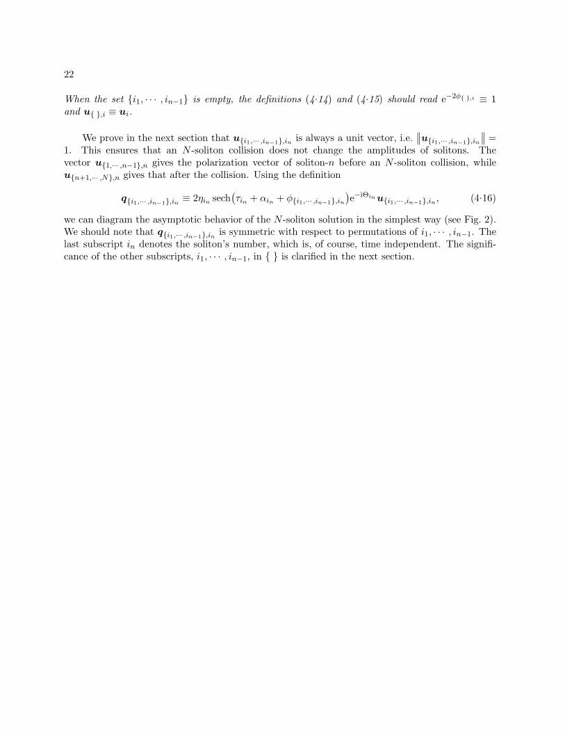
1. This ensures that an N -soliton collision does not change the amplitudes of solitons. Thevector u{1,··· ,n−1},n gives the polarization vector of soliton-n before an N -soliton collision, whileu{n+1,··· ,N},n gives that after the collision. Using the definition

q{i1,··· ,in−1},in ≡ 2ηin sech(τin + αin + φ{i1,··· ,in−1},in

)e−iΘinu{i1,··· ,in−1},in , (4.16)

we can diagram the asymptotic behavior of the N -soliton solution in the simplest way (see Fig. 2).We should note that q{i1,··· ,in−1},in is symmetric with respect to permutations of i1, · · · , in−1. Thelast subscript in denotes the soliton’s number, which is, of course, time independent. The signifi-cance of the other subscripts, i1, · · · , in−1, in { } is clarified in the next section.

23

interactionranget

1

N1 n

N n

q{1,...,N−1},N q{1,...,n−1},n q{ },1

q{2,...,N},1 q{n+1,...,N},n q{ },N

Fig. 2. Asymptotic behavior of the N-soliton solution.

24

§5. Factorization of an N-soliton collision into a superposition of pair collisions

In this section, on the basis of the collision laws of two solitons presented in §3, we examine theasymptotic behavior of the N -soliton solution obtained in §4. We conclude that an N -soliton colli-sion in the Manakov model (1.1) can be factorized into a nonlinear superposition of pair collisionsin arbitrary order.

We first prove a lemma needed later to compute the Hermitian product of u{i1,··· ,in−1},j andu{i1,··· ,in−1},k.

Lemma 5.1. For any set of unit vectors ui1 , · · · ,uin−1 ,uj ,uk and dil defined by (4.8), the followingequality holds:

∣∣∣∣∣∣∣∣∣

di1i1 · · · di1in−1 ui1...

. . ....

...

din−1i1 · · · din−1in−1 uin−1

dji1 · · · djin−1 uj

∣∣∣∣∣∣∣∣∣

·

∣∣∣∣∣∣∣∣∣

di1i1 · · · di1in−1 ui1...

. . ....

...

din−1i1 · · · din−1in−1 uin−1

dki1 · · · dkin−1 uk

∣∣∣∣∣∣∣∣∣

†

=ζk − ζ∗j

i×

∣∣∣∣∣∣∣

di1i1 · · · di1in−1

.... . .

...

din−1i1 · · · din−1in−1

∣∣∣∣∣∣∣

×

∣∣∣∣∣∣∣∣∣

di1i1 · · · di1in−1 di1k...

. . ....

...

din−1i1 · · · din−1in−1 din−1k

dji1 · · · djin−1 djk

∣∣∣∣∣∣∣∣∣

. (5.1)

Proof. In the proof of this lemma, we use D to denote the last determinant in (5.1):

D ≡

∣∣∣∣∣∣∣∣∣

di1i1 · · · di1in−1 di1k...

. . ....

...din−1i1 · · · din−1in−1 din−1k

dji1 · · · djin−1 djk

∣∣∣∣∣∣∣∣∣

.

We express minor determinants obtained by deleting one row and one column of D as

D

[ilk

]

=

∣∣∣∣∣∣∣∣∣∣∣∣∣∣∣∣

di1i1 · · · di1in−1

......

dil−1i1 · · · dil−1in−1

dil+1i1 · · · dil+1in−1

......

din−1i1 · · · din−1in−1

dji1 · · · djin−1

∣∣∣∣∣∣∣∣∣∣∣∣∣∣∣∣

,

D

[jil

]

=

∣∣∣∣∣∣∣

di1i1 · · · di1il−1di1il+1

· · · di1in−1 di1k...

......

......

din−1i1 · · · din−1il−1din−1il+1

· · · din−1in−1 din−1k

∣∣∣∣∣∣∣

,

25

D

[jk

]

=

∣∣∣∣∣∣∣

di1i1 · · · di1in−1

.... . .

...din−1i1 · · · din−1in−1

∣∣∣∣∣∣∣

.

Using these abbreviations and the Laplace expansion of determinants, we can rewrite the left-handside of (5.1) as

l.h.s. =

n−1∑

p=1

(−1)n+pD

[ipk

]

uip +D

[jk

]

uj

·

n−1∑

q=1

(−1)n+qD

[jiq

]

u†iq+D

[jk

]

u†k

=

n−1∑

p=1

n−1∑

q=1

(−1)p+qD

[ipk

]

D

[jiq

]

×

{

(ζiq − ζ∗j ) + (ζ∗j − ζ∗ip)

i

}

dipiq

+

n−1∑

q=1

(−1)n+qD

[jk

]

D

[jiq

]

×(ζiq − ζ∗j )

idjiq

+n−1∑

p=1

(−1)n+pD

[ipk

]

D

[jk

]

×

{

(ζk − ζ∗j ) + (ζ∗j − ζ∗ip)

i

}

dipk

+D

[jk

]

D

[jk

]

×(ζk − ζ∗j )

idjk

=n−1∑

q=1

(−1)n+qD

[jiq

](ζiq − ζ∗j )

i

n−1∑

p=1

(−1)n+pD

[ipk

]

dipiq +D

[jk

]

djiq

+

n−1∑

p=1

(−1)n+pD

[ipk

](ζ∗j − ζ∗ip)

i

n−1∑

q=1

(−1)n+qD

[jiq

]

dipiq +D

[jk

]

dipk

+D

[jk

](ζk − ζ∗j )

i

n−1∑

p=1

(−1)n+pD

[ipk

]

dipk +D

[jk

]

djk

=

n−1∑

q=1

(−1)n+qD

[jiq

](ζiq − ζ∗j )

i

∣∣∣∣∣∣∣∣∣

di1i1 · · · di1in−1 di1iq...

. . ....

...din−1i1 · · · din−1in−1 din−1iq

dji1 · · · djin−1 djiq

∣∣∣∣∣∣∣∣∣

+n−1∑

p=1

(−1)n+pD

[ipk

](ζ∗j − ζ∗ip)

i

∣∣∣∣∣∣∣∣∣

di1i1 · · · di1in−1 di1k...

. . ....

...din−1i1 · · · din−1in−1 din−1k

dipi1 · · · dipin−1 dipk

∣∣∣∣∣∣∣∣∣

+D

[jk

](ζk − ζ∗j )

iD.

26

It is easily seen that in the last expression, only the last term remains. This is the right-hand sideof (5.1). �

Corollary 5.2. The vector u{i1,··· ,in−1},in defined for distinct positive integers i1, · · · , in−1, in by

(4.15) with (4.14) is a unit vector, i.e.∣∣∣∣u{i1,··· ,in−1},in

∣∣∣∣ = 1.

Proof. Using Lemma 5.1 in the special case j = k (≡ in), we have∣∣∣∣u{i1,··· ,in−1},in

∣∣∣∣2 = u{i1,··· ,in−1},in · u†

{i1,··· ,in−1},in

=n−1∏

l=1

∣∣∣∣

ζil − ζ∗inζil − ζin

∣∣∣∣

2

×

dinin

∣∣∣∣∣∣∣

di1i1 · · · di1in−1

.... . .

...din−1i1 · · · din−1in−1

∣∣∣∣∣∣∣

∣∣∣∣∣∣∣

di1i1 · · · di1in...

. . ....

dini1 · · · dinin

∣∣∣∣∣∣∣

×

n−1∏

l=1

∣∣∣∣

ζ∗il − ζ∗inζil − ζ∗in

∣∣∣∣

2

×

ζin − ζ∗ini

∣∣∣∣∣∣∣

di1i1 · · · di1in−1

.... . .

...din−1i1 · · · din−1in−1

∣∣∣∣∣∣∣

∣∣∣∣∣∣∣

di1i1 · · · di1in...

. . ....

dini1 · · · dinin

∣∣∣∣∣∣∣

∣∣∣∣∣∣∣

di1i1 · · · di1in−1

.... . .

...din−1i1 · · · din−1in−1

∣∣∣∣∣∣∣

2

= 1. �

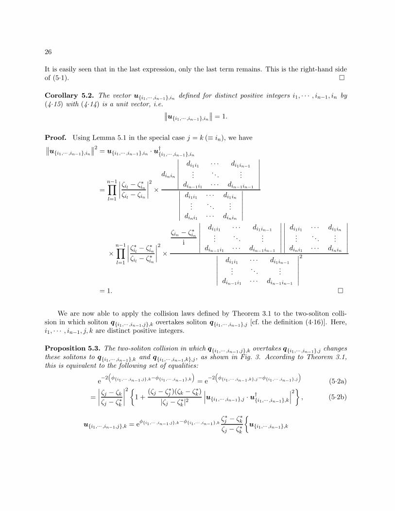
We are now able to apply the collision laws defined by Theorem 3.1 to the two-soliton colli-sion in which soliton q{i1,··· ,in−1,j},k overtakes soliton q{i1,··· ,in−1},j [cf. the definition (4.16)]. Here,i1, · · · , in−1, j, k are distinct positive integers.

Proposition 5.3. The two-soliton collision in which q{i1,··· ,in−1,j},k overtakes q{i1,··· ,in−1},j changes

these solitons to q{i1,··· ,in−1},k and q{i1,··· ,in−1,k},j, as shown in Fig. 3. According to Theorem 3.1,

this is equivalent to the following set of equalities:

e−2(

φ{i1,··· ,in−1,j},k−φ{i1,··· ,in−1},k

)

= e−2(

φ{i1,··· ,in−1,k},j−φ{i1,··· ,in−1},j

)

(5.2a)

=

∣∣∣∣

ζj − ζkζj − ζ∗k

∣∣∣∣

2{

1 +(ζj − ζ∗j )(ζk − ζ∗k)

|ζj − ζ∗k |2

∣∣∣u{i1,··· ,in−1},j · u

†{i1,··· ,in−1},k

∣∣∣

2}

, (5.2b)

u{i1,··· ,in−1,j},k = eφ{i1,··· ,in−1,j},k

−φ{i1,··· ,in−1},kζ∗j − ζ∗kζj − ζ∗k

{

u{i1,··· ,in−1},k

27

−ζj − ζ∗jζj − ζ∗k

(

u{i1,··· ,in−1},k · u†{i1,··· ,in−1},j

)

u{i1,··· ,in−1},j

}

, (5.3)

u{i1,··· ,in−1,k},j = eφ{i1,··· ,in−1,k},j

−φ{i1,··· ,in−1},jζ∗k − ζ∗jζk − ζ∗j

{

u{i1,··· ,in−1},j

−ζk − ζ∗kζk − ζ∗j

(

u{i1,··· ,in−1},j · u†{i1,··· ,in−1},k

)

u{i1,··· ,in−1},k

}

. (5.4)

Proof. Throughout this proof, we employ the following notation in order to express determinantscompactly:

d

(j1, j2, · · · , jlk1, k2, · · · , kl

)

≡

∣∣∣∣∣∣∣∣∣

dj1k1 dj1k2 · · · dj1kldj2k1 dj2k2 · · · dj2kl...

.... . .

...djlk1 djlk2 · · · djlkl

∣∣∣∣∣∣∣∣∣

.

To prove (5.2), we first rewrite the left-hand side of (5.2a) as

e−2(

φ{i1,··· ,in−1,j},k−φ{i1,··· ,in−1},k

)

=

∣∣∣∣

ζj − ζkζj − ζ∗k

∣∣∣∣

2

×

d

(i1, · · · , in−1, j, ki1, · · · , in−1, j, k

)

d

(i1, · · · , in−1

i1, · · · , in−1

)

d

(i1, · · · , in−1, ji1, · · · , in−1, j

)

d

(i1, · · · , in−1, ki1, · · · , in−1, k

) , (5.5)

using the definition of φ{i1,··· ,in−1},in , (4.14). Obviously, the right-hand side of (5.5) is symmetric

with respect to interchange of j and k. It follows that the equality (5.2a) holds.Next, we prove the equality (5.2b). Using the definition of u{i1,··· ,in−1},in , (4

.15), and Lemma 5.1,we obtain

u{i1,··· ,in−1},j · u†{i1,··· ,in−1},k

= eφ{i1,··· ,in−1},j

+φ{i1,··· ,in−1},k ×ζk − ζ∗j

i×

n−1∏

l=1

(ζ∗il − ζ∗j )(ζil − ζk)

(ζil − ζ∗j )(ζ∗il− ζk)

×

d

(i1, · · · , in−1, ji1, · · · , in−1, k

)

d

(i1, · · · , in−1

i1, · · · , in−1

) . (5.6)

Multiplying (5.6) by its complex conjugate on each side, we obtain, with the help of (4.14),

∣∣∣u{i1,··· ,in−1},j · u

†{i1,··· ,in−1},k

∣∣∣

2= −

∣∣∣ζk − ζ∗j

∣∣∣

2

(ζj − ζ∗j )(ζk − ζ∗k)×

d

(i1, · · · , in−1, ji1, · · · , in−1, k

)

d

(i1, · · · , in−1, ki1, · · · , in−1, j

)

d

(i1, · · · , in−1, ji1, · · · , in−1, j

)

d

(i1, · · · , in−1, ki1, · · · , in−1, k

) .

Then, we can rewrite the right-hand side of (5.2b) as∣∣∣∣

ζj − ζkζj − ζ∗k

∣∣∣∣

2{

1 +(ζj − ζ∗j )(ζk − ζ∗k)

|ζj − ζ∗k |2

∣∣∣u{i1,··· ,in−1},j · u

†{i1,··· ,in−1},k

∣∣∣

2}

28

=

∣∣∣∣

ζj − ζkζj − ζ∗k

∣∣∣∣

2

1−

d

(i1, · · · , in−1, ji1, · · · , in−1, k

)

d

(i1, · · · , in−1, ki1, · · · , in−1, j

)

d

(i1, · · · , in−1, ji1, · · · , in−1, j

)

d

(i1, · · · , in−1, ki1, · · · , in−1, k

)

. (5.7)

Here, thanks to the Jacobi formula for determinants, we have

d

(i1, · · · , in−1, ji1, · · · , in−1, j

)

d

(i1, · · · , in−1, ki1, · · · , in−1, k

)

− d

(i1, · · · , in−1, ji1, · · · , in−1, k

)

d

(i1, · · · , in−1, ki1, · · · , in−1, j

)

= d

(i1, · · · , in−1

i1, · · · , in−1

)

d

(i1, · · · , in−1, j, ki1, · · · , in−1, j, k

)

. (5.8)

Thus, (5.7) is equal to (5.5). This completes the proof of the equality (5.2b).To prove the equality (5.3), we need to extend the Jacobi formula (5.8). We remark that,

although the matrix elements dil here are given by (4.8), the two sides of (5.8) are equal as apolynomial for general elements dil. Therefore, maintaining the validity of (5.8), we can replacethe columns with index k by columns consisting of the vectors ui1 , · · · ,uin−1 ,uj or uk:

d

(i1, · · · , in−1, ji1, · · · , in−1, j

)

∣∣∣∣∣∣∣∣∣

di1i1 · · · di1in−1 ui1...

. . ....

...din−1i1 · · · din−1in−1 uin−1

dki1 · · · dkin−1 uk

∣∣∣∣∣∣∣∣∣

− d

(i1, · · · , in−1, ki1, · · · , in−1, j

)

×

∣∣∣∣∣∣∣∣∣

di1i1 · · · di1in−1 ui1...

. . ....

...din−1i1 · · · din−1in−1 uin−1

dji1 · · · djin−1 uj

∣∣∣∣∣∣∣∣∣

= d

(i1, · · · , in−1

i1, · · · , in−1

)

∣∣∣∣∣∣∣∣∣∣∣

di1i1 · · · di1in−1 di1j ui1...

. . ....

......

din−1i1 · · · din−1in−1 din−1j uin−1

dji1 · · · djin−1 djj uj

dki1 · · · dkin−1 dkj uk

∣∣∣∣∣∣∣∣∣∣∣

.

(5.9)

We rewrite the right-hand side of (5.3) using (4.14), (4.15) and (5.6) (with j ↔ k) as

eφ{i1,··· ,in−1,j},k

−φ{i1,··· ,in−1},kζ∗j − ζ∗kζj − ζ∗k

{

u{i1,··· ,in−1},k −ζj − ζ∗jζj − ζ∗k

(

u{i1,··· ,in−1},k · u†{i1,··· ,in−1},j

)

× u{i1,··· ,in−1},j

}

= eφ{i1,··· ,in−1,j},k ×

ζ∗j − ζ∗kζj − ζ∗k

n−1∏

l=1

ζ∗il − ζ∗kζil − ζ∗k

×1

d

(i1, · · · , in−1, ji1, · · · , in−1, j

)

d

(i1, · · · , in−1

i1, · · · , in−1

)

×

d

(i1, · · · , in−1, ji1, · · · , in−1, j

)

∣∣∣∣∣∣∣∣∣

di1i1 · · · di1in−1 ui1...

. . ....

...din−1i1 · · · din−1in−1 uin−1

dki1 · · · dkin−1 uk

∣∣∣∣∣∣∣∣∣

− d

(i1, · · · , in−1, ki1, · · · , in−1, j

)

29

×

∣∣∣∣∣∣∣∣∣

di1i1 · · · di1in−1 ui1...

. . ....

...din−1i1 · · · din−1in−1 uin−1

dji1 · · · djin−1 uj

∣∣∣∣∣∣∣∣∣

.

Owing to the extended Jacobi formula (5.9), this is equal to u{i1,··· ,in−1,j},k [cf. the definition (4.15)].Now, the proof of the equality (5.3) is complete. The proof of the equality (5.4) is obtained byinterchanging j and k in the proof of (5.3). �

Proposition 5.3 is applicable to two-soliton collisions satisfying the following condition:• Before the collision, the set of subscripts in the left-hand soliton’s { } is equal to the entire

set of subscripts of the right-hand soliton: {i1, · · · , in−1, j} = {i1, · · · , in−1} ∪ {j}.We also note the following properties (cf. Fig. 3):

• After the collision, the set of subscripts in the left-hand soliton’s { } is still equal to the entireset of subscripts of the right-hand soliton: {i1, · · · , in−1, k} = {i1, · · · , in−1} ∪ {k}.

• The entire set of subscripts of the left-hand soliton is unchanged: {i1, · · · , in−1, j} ∪ {k} ={i1, · · · , in−1, k} ∪ {j}.

• The set of subscripts in the right-hand soliton’s { } is unchanged: {i1, · · · , in−1} = {i1, · · · , in−1}.• The overtaken soliton’s number is removed from the overtaking soliton’s { }, while the over-

taking soliton’s number is added to the overtaken soliton’s { }.

30

interactionrange

soliton-

soliton-

t

soliton-

soliton-

k j

j k

q{i1,...,in−1,j},kq{i1,...,in−1},j

q{i1,...,in−1,k},jq{i1,...,in−1},k

Fig. 3. Two-soliton collision in the presence of other solitons.

31

We are now able to state the main result of this paper.

Theorem 5.4. An N -soliton collision in the Manakov model (1.1) can be factorized into a nonlinear

superposition of(N2

)pair collisions in arbitrary order.

Proof. According to the asymptotic behavior of the N -soliton solution as t → −∞ (see Fig. 2),solitons-N , · · · , 1 are initially distributed along the x-axis as

q{1,··· ,N−1},N , · · · , q{1,··· ,n−1},n, · · · , q{ },1.

We take this initial state as the point of departure and assume that the solitons collide pairwise in

a given order. Then, a pair collision takes place(N2

)= N(N−1)

2 times. What will the final state beunder this assumption? To answer this, we note the following two points:

• The set of subscripts in each soliton’s { } is always equal to the entire set of subscripts of thenext soliton to the right. This ensures that Proposition 5.3 is applicable to every pair collision.

• Soliton-n will overtake solitons-1, · · · , n− 1 and will be overtaken by solitons-n + 1, · · · , N .We see that, regardless of the order of the pair collisions, solitons-1, · · · , N are finally distributedalong the x-axis as

q{2,··· ,N},1, · · · , q{n+1,··· ,N},n, · · · , q{ },N .

This final state is exactly the same as the asymptotic behavior of the N -soliton solution in thet → +∞ limit (see Fig. 2).

Q.E.D.

Remark 1. Theorem 5.4, together with (3.10), demonstrates that the initial state of N solitonsuniquely determines its final state. That is, an N -soliton collision described by Proposition 4.2defines a mapping from the initial state to the final state. This fact is not evident from Proposi-tion 4.2.

Remark 2. We can now prove that the mapping (3.10) satisfies the property (b) or, equivalentlythe Yang-Baxter property (b’), as stated in the introduction. It is sufficient to verify the following:

The initial polarization vectors of N solitons (u{1,··· ,N−1},N , · · · ,u{ },1) given inProposition 4.2 can be made to coincide with any combination of N unit vectors inCm by appropriately varying the bare polarization vectors (uN , · · · ,u1).

This is easily verified if we consider the order of the pair collisions such that every soliton ex-periences the bare polarization u{ },j(= uj) once and inductively use the fact that the mappingu2 7→ u{1},2 in Theorem 3.1 is a bijection on the unit sphere.

Remark 3. The validity of the Yang-Baxter property allows us to extract a new “set-theoretical”solution to the quantum Yang-Baxter equation (cf. Refs. 15) and 16)). To be more specific, re-garding (3.10) as the mapping (u{1},2,u1) 7→ (u2,u{2},1), we obtain a nontrivial solution to theparameter-dependent Yang-Baxter equation for mappings that act on the direct product of two(complex) unit vectors. Naturally, we can extend this solution further by adding information con-

32

cerning the center positions of solitons. However, this extension is not very intriguing, because thenet change wrought by the mapping does not depend on the added information.

§6. Concluding remarks

In this paper, we have investigated soliton collisions in the Manakov model for the general caseof m components (1.1) using a straightforward approach. We first derived the general N -solitonsolution of the Manakov model from that of the matrix NLS equation (2.2) through a simplereduction.14) We considered the limits t → ∓∞ for the N = 2 case and obtained the collision lawsof two solitons in the Manakov model. Next, we considered the same limits for the case of generalN and obtained the asymptotic behavior of the N -soliton solution. We were able to diagram theasymptotic behavior in the simplest way in terms of the quantity q{i1,··· ,in−1},in defined by (4.16)(see Fig. 2). Taking advantage of this, we proved with a simple combinatorial treatment that anN -soliton collision in the Manakov model can be factorized into a nonlinear superposition of

(N2

)

pair collisions in arbitrary order. This clears up the longtime misunderstanding that multi-particleeffects exist in the Manakov model.

This result is far from trivial in the m ≥ 2 case. In the m = 1 case (scalar NLS), all thesoliton parameters that play an essential role in the collision laws (in the notation of this paper,ζ1, ζ2, · · · , ζN ) are invariant in time. A pair collision results only in a displacement of the solitoncenters and a shift of the phases, which will not change the effects of future pair collisions. Thus, asuperposition of

(N2

)pair collisions gives the same results for every order of the pair collisions. It

is not difficult to prove in this case that an N -soliton collision reduces to a pair collision.10), 11), 12)

In contrast, in the m ≥ 2 case, a pair collision results in a change of the polarization vectors. Thischanges the effects of future pair collisions completely. Therefore, it was not obvious before thepresent work that a nonlinear superposition of

(N2

)pair collisions gives the same results for every

order of the pair collisions or that it exactly coincides with an N -soliton collision. The key toproving these facts is a highly nontrivial relation among determinants and extended determinants,given in Lemma 5.1. This implies the possibility that some new relations similar to Lemma 5.1 canbe obtained through the investigation of soliton collisions in multi-component integrable systems.

Very recently, Steiglitz and coworkers36), 37) proposed that soliton collisions in the Manakovmodel can be utilized to carry out any computation with beams in a nonlinear optical medium(see Ref. 38) for the experimental foundations). We believe that the results obtained in this paperwill be useful to refine and reinforce their interesting idea. In particular, Theorem 5.4 supports∗)

their hypothesis on the pairwise nature of soliton collisions and Proposition 4.2, together withProposition 5.3, provides a hint on how to design optical logic operations more simply and reliablythan the method proposed in Ref. 37).

∗) To be precise, we need to extend our result to the case in which some solitons propagate at the same velocity

and do not collide with one another. This is beyond the scope of this paper and is left to the reader as a future

problem.

33

Acknowledgements

The author is grateful to Prof. Miki Wadati, Prof. Ryu Sasaki, Prof. Tetsuji Tokihiro, Prof.Jianke Yang, Dr. Ken-ichi Maruno and anonymous referees for their useful comments. This researchwas supported in part by a JSPS Research Fellowship for Young Scientists.

References

1) C. R. Menyuk, IEEE J. Quantum Electron. 25 (1989), 2674.2) G. P. Agrawal, Nonlinear Fiber Optics, 2nd ed. (Academic Press, San Diego, 1995).3) N. N. Akhmediev and A. Ankiewicz, Solitons: Nonlinear pulses and beams (Chapman & Hall, London,

1997).4) S. V. Manakov, Sov. Phys. -JETP 38 (1974), 248.5) V. G. Makhan’kov and O. K. Pashaev, Theor. Math. Phys. 53 (1982), 979.6) R. Radhakrishnan, M. Lakshmanan and J. Hietarinta, Phys. Rev. E 56 (1997), 2213.7) V. Shchesnovich, solv-int/9712020.8) J. Yang, Phys. Rev. E 59 (1999), 2393.9) J. P. Silmon-Clyde and J. N. Elgin, J. Opt. Soc. Am. B 16 (1999), 1348.

10) V. E. Zakharov and A. B. Shabat, Sov. Phys. -JETP 34 (1972), 62.11) S. Novikov, S. V. Manakov, L. P. Pitaevskii and V. E. Zakharov, Theory of Solitons: The Inverse Scattering

Method (Consultants Bureau, New York, 1984).12) L. D. Faddeev and L. A. Takhtajan, Hamiltonian Methods in the Theory of Solitons (Springer, Berlin, 1987).13) T. Tsuchida and M. Wadati, J. Phys. Soc. Jpn. 67 (1998), 1175.14) T. Tsuchida, “Study of multi-component soliton equations based on the inverse scattering method”, Ph.D

thesis, Department of Physics, University of Tokyo (2000), available athttp://poisson.ms.u-tokyo.ac.jp/˜tsuchida/thesis/

15) V. G. Drinfeld, Lecture Notes in Math., Vol. 1510 (Springer, Berlin, 1992) p. 1.16) A. P. Veselov, Phys. Lett. A 314 (2003), 214.17) V. E. Zakharov, Sov. Phys. -JETP 33 (1971), 538.18) P. P. Kulish, Theor. Math. Phys. 26 (1976), 132.19) V. M. Goncharenko, Theor. Math. Phys. 126 (2001), 81.20) Y. Ohta, RIMS kokyuroku 684 (1989), 1 [in Japanese].21) K. W. Chow and D. W. C. Lai, J. Phys. Soc. Jpn. 67 (1998), 3721.22) M. J. Ablowitz, Y. Ohta and A. D. Trubatch, Phys. Lett. A 253 (1999), 287.23) Y. Nogami and C. S. Warke, Phys. Lett. A 59 (1976), 251.24) A. A. Sukhorukov and N. N. Akhmediev, nlin.PS/0208043.25) Q-H. Park and H. J. Shin, IEEE J. Sel. Top. Quantum Electron. 8 (2002), 432.26) A. Borah, S. Ghosh and S. Nandy, Eur. Phys. J. B 29 (2002), 221.27) T. Kanna and M. Lakshmanan, Phys. Rev. E 67 (2003), 046617.28) H. Steudel, J. Mod. Opt. 35 (1988), 693.29) T. Tsuchida, J. of Phys. A 35 (2002), 7827.30) V. S. Gerdzhikov and M. I. Ivanov, Theor. Math. Phys. 52 (1982), 676.31) T. Tsuchida, H. Ujino and M. Wadati, J. of Phys. A 32 (1999), 2239.32) O. O. Vakhnenko, J. of Phys. A 32 (1999), 5735.33) I. Kay and H. E. Moses, J. Appl. Phys. 27 (1956), 1503.34) M. Wadati and M. Toda, J. Phys. Soc. Jpn. 32 (1972), 1403.35) C. S. Gardner, J. M. Greene, M. D. Kruskal and R. M. Miura, Commun. Pure Appl. Math. 27 (1974), 97.36) M. H. Jakubowski, K. Steiglitz and R. Squier, Phys. Rev. E 58 (1998), 6752.37) K. Steiglitz, Phys. Rev. E 63 (2001), 016608.38) C. Anastassiou, J. W. Fleischer, T. Carmon, M. Segev and K. Steiglitz, Opt. Lett. 26 (2001), 1498.