mws gen reg ppt nonlinear - USF College of...
22
10/22/2014 http://numericalmethods.eng.usf.edu 1 10/22/2014 http://numericalmethods.eng.usf.edu 1 Nonlinear Regression Major: All Engineering Majors Authors: Autar Kaw, Luke Snyder http://numericalmethods.eng.usf.edu Transforming Numerical Methods Education for STEM Undergraduates Nonlinear Regression http://numericalmethods.eng.usf.edu
-
Upload
nguyendung -
Category
Documents
-
view
221 -
download
0
Transcript of mws gen reg ppt nonlinear - USF College of...
10/22/2014
http://numericalmethods.eng.usf.edu 1
10/22/2014 http://numericalmethods.eng.usf.edu 1
Nonlinear Regression
Major: All Engineering Majors
Authors: Autar Kaw, Luke Snyder
http://numericalmethods.eng.usf.eduTransforming Numerical Methods Education for STEM
Undergraduates
Nonlinear Regression
http://numericalmethods.eng.usf.edu
10/22/2014
http://numericalmethods.eng.usf.edu 2
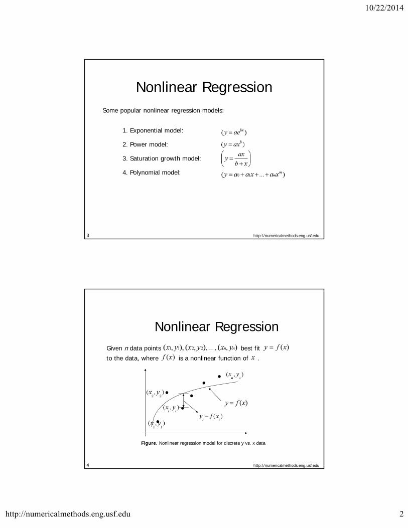
Nonlinear RegressionSome popular nonlinear regression models:
1. Exponential model:
2. Power model:
3. Saturation growth model:
4. Polynomial model:
http://numericalmethods.eng.usf.edu3
Nonlinear RegressionGiven n data points best fit
to the data, where is a nonlinear function of .
Figure. Nonlinear regression model for discrete y vs. x data
http://numericalmethods.eng.usf.edu4

10/22/2014
http://numericalmethods.eng.usf.edu 3
RegressionExponential Model
http://numericalmethods.eng.usf.edu5
Exponential ModelGiven best fit to the data.
Figure. Exponential model of nonlinear regression for y vs. x data
http://numericalmethods.eng.usf.edu6
10/22/2014
http://numericalmethods.eng.usf.edu 4
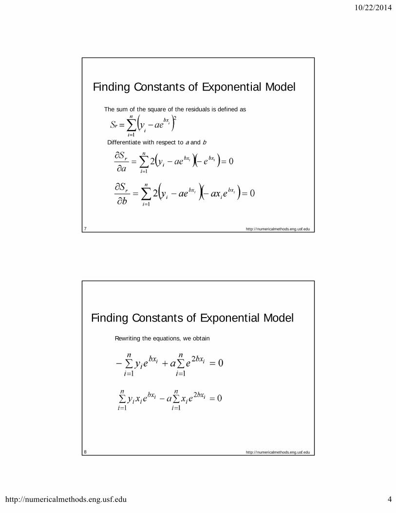
Finding Constants of Exponential Model
The sum of the square of the residuals is defined as
Differentiate with respect to a and b
http://numericalmethods.eng.usf.edu7
Finding Constants of Exponential Model
Rewriting the equations, we obtain
http://numericalmethods.eng.usf.edu8

10/22/2014
http://numericalmethods.eng.usf.edu 5
Finding constants of Exponential Model
Substituting a back into the previous equation
The constant b can be found through numerical methods such as bisection method.
Solving the first equation for a yields
http://numericalmethods.eng.usf.edu9
Example 1-Exponential Model
t(hrs) 0 1 3 5 7 9
1.000 0.891 0.708 0.562 0.447 0.355
Many patients get concerned when a test involves injection of a radioactive material. For example for scanning a gallbladder, a few drops of Technetium-99m isotope is used. Half of the Technitium-99m would be gone in about 6 hours. It, however, takes about 24 hours for the radiation levels to reach what we are exposed to in day-to-day activities. Below is given the relative intensity of radiation as a function of time.
Table. Relative intensity of radiation as a function of time.
http://numericalmethods.eng.usf.edu10

10/22/2014
http://numericalmethods.eng.usf.edu 6
Example 1-Exponential Model cont.
Find: a) The value of the regression constants and
b) The half-life of Technetium-99m
c) Radiation intensity after 24 hours
The relative intensity is related to time by the equation
http://numericalmethods.eng.usf.edu11
Plot of data
http://numericalmethods.eng.usf.edu12

10/22/2014
http://numericalmethods.eng.usf.edu 7
Constants of the Model
The value of λ is found by solving the nonlinear equation
http://numericalmethods.eng.usf.edu13
Setting up the Equation in MATLAB
t (hrs) 0 1 3 5 7 9γ 1.000 0.891 0.708 0.562 0.447 0.355
http://numericalmethods.eng.usf.edu14

10/22/2014
http://numericalmethods.eng.usf.edu 8
Setting up the Equation in MATLAB
t=[0 1 3 5 7 9]gamma=[1 0.891 0.708 0.562 0.447 0.355]syms lamdasum1=sum(gamma.*t.*exp(lamda*t));sum2=sum(gamma.*exp(lamda*t));sum3=sum(exp(2*lamda*t));sum4=sum(t.*exp(2*lamda*t));f=sum1-sum2/sum3*sum4;
http://numericalmethods.eng.usf.edu15
Calculating the Other Constant
The value of A can now be calculated
The exponential regression model then is
http://numericalmethods.eng.usf.edu16

10/22/2014
http://numericalmethods.eng.usf.edu 9
Plot of data and regression curve
http://numericalmethods.eng.usf.edu17
Relative Intensity After 24 hrs
The relative intensity of radiation after 24 hours
This result implies that only
radioactive intensity is left after 24 hours.
http://numericalmethods.eng.usf.edu18

10/22/2014
http://numericalmethods.eng.usf.edu 10
Homework• What is the half-life of Technetium-99m
isotope?• Write a program in the language of your
choice to find the constants of the model.
• Compare the constants of this regression model with the one where the data is transformed.
• What if the model was ?
http://numericalmethods.eng.usf.edu19
THE END
http://numericalmethods.eng.usf.eduhttp://numericalmethods.eng.usf.edu20

10/22/2014
http://numericalmethods.eng.usf.edu 11
Polynomial Model
Given best fit
to a given data set.
Figure. Polynomial model for nonlinear regression of y vs. x data
http://numericalmethods.eng.usf.edu21
Polynomial Model cont.The residual at each data point is given by
The sum of the square of the residuals then is
http://numericalmethods.eng.usf.edu22

10/22/2014
http://numericalmethods.eng.usf.edu 12
Polynomial Model cont.To find the constants of the polynomial model, we set the derivatives with respect to where equal to zero.
http://numericalmethods.eng.usf.edu23
Polynomial Model cont.These equations in matrix form are given by
The above equations are then solved for
http://numericalmethods.eng.usf.edu24
10/22/2014
http://numericalmethods.eng.usf.edu 13
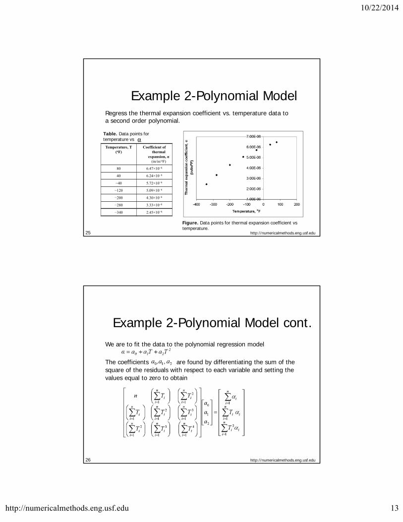
Example 2-Polynomial Model
Temperature, T(oF)
Coefficient of thermal
expansion, α (in/in/oF)
80 6.47×10⁻⁶
40 6.24×10⁻⁶
−40 5.72×10⁻⁶
−120 5.09×10⁻⁶
−200 4.30×10⁻⁶
−280 3.33×10⁻⁶
−340 2.45×10⁻⁶
Regress the thermal expansion coefficient vs. temperature data to a second order polynomial.
Table. Data points for temperature vs
Figure. Data points for thermal expansion coefficient vs temperature.
http://numericalmethods.eng.usf.edu25
Example 2-Polynomial Model cont.We are to fit the data to the polynomial regression model
The coefficients are found by differentiating the sum of thesquare of the residuals with respect to each variable and setting thevalues equal to zero to obtain
http://numericalmethods.eng.usf.edu26

10/22/2014
http://numericalmethods.eng.usf.edu 14
Example 2-Polynomial Model cont.The necessary summations are as follows
Temperature, T(oF)
Coefficient of thermal expansion,
α (in/in/oF)
80 6.47×10⁻⁶
40 6.24×10⁻⁶
−40 5.72×10⁻⁶
−120 5.09×10⁻⁶
−200 4.30×10⁻⁶
−280 3.33×10⁻⁶
−340 2.45×10⁻⁶
Table. Data points for temperature vs.
http://numericalmethods.eng.usf.edu27
Example 2-Polynomial Model cont.Using these summations, we can now calculate
Solving the above system of simultaneous linear equations we have
The polynomial regression model is then
http://numericalmethods.eng.usf.edu28

10/22/2014
http://numericalmethods.eng.usf.edu 15
Transformation of DataTo find the constants of many nonlinear models, it results in solving simultaneous nonlinear equations. For mathematical convenience, some of the data for such models can be transformed. For example, the data for an exponential model can be transformed.
As shown in the previous example, many chemical and physical processes are governed by the equation,
Taking the natural log of both sides yields,
Let and
(implying) with
We now have a linear regression model where
http://numericalmethods.eng.usf.edu29
Transformation of data cont.Using linear model regression methods,
Once are found, the original constants of the model are found as
http://numericalmethods.eng.usf.edu30

10/22/2014
http://numericalmethods.eng.usf.edu 16
THE END
http://numericalmethods.eng.usf.eduhttp://numericalmethods.eng.usf.edu31
Example 3-Transformation of data
t(hrs) 0 1 3 5 7 9
1.000 0.891 0.708 0.562 0.447 0.355
Many patients get concerned when a test involves injection of a radioactive material. For example for scanning a gallbladder, a few drops of Technetium-99m isotope is used. Half of the technetium-99m would be gone in about 6hours. It, however, takes about 24 hours for the radiation levels to reach what we are exposed to in day-to-day activities. Below is given the relative intensity of radiation as a function of time.
Table. Relative intensity of radiation as a function of time
Figure. Data points of relative radiation intensityvs. time
http://numericalmethods.eng.usf.edu32

10/22/2014
http://numericalmethods.eng.usf.edu 17
Example 3-Transformation of data cont.
Find: a) The value of the regression constants and
b) The half-life of Technium-99m
c) Radiation intensity after 24 hours
The relative intensity is related to time by the equation
http://numericalmethods.eng.usf.edu33
Example 3-Transformation of data cont.
Exponential model given as,
Assuming , and we obtain
This is a linear relationship between and
http://numericalmethods.eng.usf.edu34

10/22/2014
http://numericalmethods.eng.usf.edu 18
Example 3-Transformation of data cont.
Using this linear relationship, we can calculate
and
where
http://numericalmethods.eng.usf.edu35
Example 3-Transformation of Data cont.
123456
013579
10.8910.7080.5620.4470.355
0.00000−0.11541−0.34531−0.57625−0.80520−1.0356
0.0000−0.11541−1.0359−2.8813−5.6364−9.3207
0.00001.00009.000025.00049.00081.000
25.000 −2.8778 −18.990 165.00
Summations for data Transformation are as follows
Table. Summation data for Transformation of data model
With
http://numericalmethods.eng.usf.edu36
10/22/2014
http://numericalmethods.eng.usf.edu 19
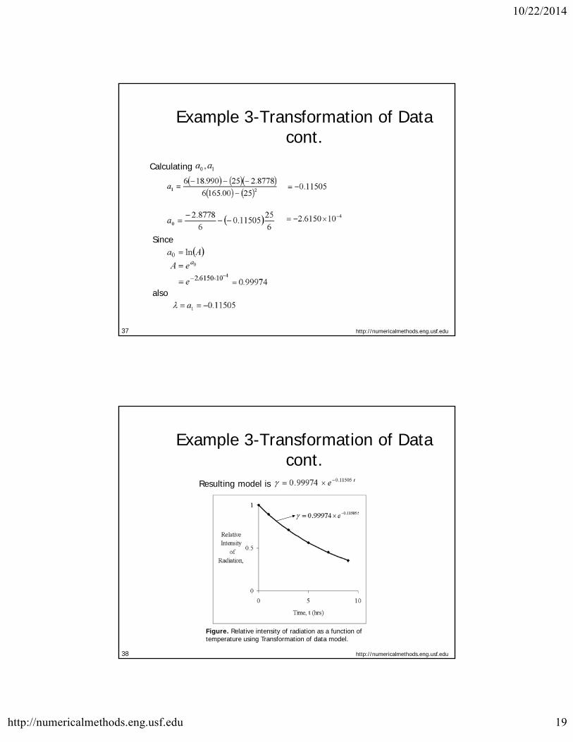
Example 3-Transformation of Data cont.
Calculating
Since
also
http://numericalmethods.eng.usf.edu37
Example 3-Transformation of Data cont.
Resulting model is
Figure. Relative intensity of radiation as a function of temperature using Transformation of data model.
http://numericalmethods.eng.usf.edu38

10/22/2014
http://numericalmethods.eng.usf.edu 20
Example 3-Transformation of Data cont.
The regression formula is then
b) Half life of Technetium 99 is when
http://numericalmethods.eng.usf.edu39
Example 3-Transformation of Data cont.
c) The relative intensity of radiation after 24 hours is then
This implies that only of the radioactive
material is left after 24 hours.
http://numericalmethods.eng.usf.edu40

10/22/2014
http://numericalmethods.eng.usf.edu 21
Comparison Comparison of exponential model with and without data Transformation:
With data Transformation
(Example 3)
Without data Transformation
(Example 1)
A 0.99974 0.99983
λ −0.11505 −0.11508
Half-Life (hrs) 6.0248 6.0232
Relative intensity after 24 hrs.
6.3200×10⁻² 6.3160×10⁻²
Table. Comparison for exponential model with and without dataTransformation.
http://numericalmethods.eng.usf.edu41
Additional ResourcesFor all resources on this topic such as digital audiovisual lectures, primers, textbook chapters, multiple-choice tests, worksheets in MATLAB, MATHEMATICA, MathCad and MAPLE, blogs, related physical problems, please visit
http://numericalmethods.eng.usf.edu/topics/nonlinear_regression.html

10/22/2014
http://numericalmethods.eng.usf.edu 22
THE END
http://numericalmethods.eng.usf.edu