
Mutations (Nachman & Crowell)
7
Department of Biomedical Informatics Harvard Medical School Broad Institute of M.I.T. and Harvard Intro to population genetics Shamil Sunyaev Forces responsible for genetic change Mutation μ Selection s N e Drift Population structure F ST Mutations Mutation rate in humans and flies ~70 per nt changes genome 2.5x10 -8 (Nachman & Crowell) 1.8x10 -8 (Kondrashov) Other events: indels (10 -9 ) repeat extensions/contractions (10 -5 ) NGS estimates ~1.2X10 -8 per nt changes genome Number of de novo mutations per individual Jonsson et al., Nature 2017 Mutation rate is variable along the genome Regional variation of mutation rate Context dependence of mutation rate Replication fidelity DNA damage DNA repair CpG deamination
Transcript of Mutations (Nachman & Crowell)

Department of Biomedical InformaticsHarvard Medical School
Broad Institute of M.I.T. and Harvard
Intro to population genetics
Shamil Sunyaev
Forces responsible for genetic change
Mutation µ
Selection s
NeDrift
Population structure FST
Mutations
Mutation rate in humans and flies
~70 per nt changes genome
2.5x10⁻⁸ (Nachman & Crowell) 1.8x10⁻⁸ (Kondrashov)
Other events: indels (10-9)
repeat extensions/contractions (10-5)
NGS estimates ~1.2X10⁻⁸ per nt changes genome
Number of de novo mutations per individual
Jonsson et al., Nature 2017
Mutation rate is variable along the genome
Regional variation of mutation rate
Context dependence of mutation rate
Replication fidelity DNA damage DNA repair CpG deamination

Genetic drift
Drift is a random change of allele frequencies
Drift depends on population size
Demographic history
Tennessen et al. Science 2012
Selection

13
NeutralDeleterious Advantageous
New mutation
Functional
Nonfunctional
Selection indicates functional mutations, whether or not the tested trait is under selection
Selective effect of mutation
Most functional mutations are deleterious
Methods of mathematical population genetics
Dynamic of allelic substitution
time0
1
Mathematically, allele frequency change in a population follows a one-dimensional random walk
Diffusion approximation
Random walk that does not jump long distances can be approximated by a diffusion process
€
∂φ x, p,t( )∂t
= −∂Mφ x, p,t( )
∂x+12∂2Vφ x, p,t( )
∂x 2
Coalescent theoryInstead of modeling a population, we can model our sample
Time goes backwards !
tNatural selection in protein
coding regions

Signatures of purifying selection
Reduced variation
Excess of rare alleles
Diversity and allele frequency
1 8 A U G U S T 2 0 1 6 | V O L 5 3 6 | N A T U R E | 2 8 7
ARTICLE RESEARCH
populations. For instance, among synonymous (non-protein- altering) variants, a class of variation expected to have undergone minimal selection, 43% of validated de novo events identified in external data sets of 1,756 parent-offspring trios8,9 are also observed independently in our data set (Fig. 2a), indicating a separate origin for the same variant within the demographic history of the two samples. This proportion is much higher for transition variants at CpG sites, well established to be the most highly mutable sites in the human genome10: 87% of previously reported de novo CpG transitions at synonymous sites are observed in ExAC, indicating that our sample sizes are beginning to approach saturation of this class of variation. This saturation is detectable by a change in the discovery rate at subsets of the ExAC data set, beginning at around 20,000 individuals (Fig. 2b), indicating that ExAC is the first human exome-wide data set, to our knowledge, large enough for this effect to be directly observed.
Mutational recurrence has a marked effect on the frequency spectrum in the ExAC data, resulting in a depletion of singletons at sites with high mutation rates (Fig. 2c). We observe a correlation between singleton rates (the proportion of variants seen only once in ExAC) and site mutability inferred from sequence context11 (r = − 0.98; P < 10−50; Extended Data Fig. 1d): sites with low predicted mutability have a singleton rate of 60%, compared to 20% for sites with the highest predicted rate (CpG transitions; Fig. 2c). Conversely, for
synonymous variants, CpG variants are approximately twice as likely to rise to intermediate frequencies: 16% of CpG variants are found in at least 20 copies in ExAC, compared to 8% of transversions and non-CpG transitions, suggesting that synonymous CpG transitions have on average two independent mutational origins in the ExAC sample. Recurrence at highly mutable sites can further be observed by examining the population sharing of doubleton synonymous variants (variants occurring in only two individuals in ExAC). Low-mutability mutations (especially transversions), are more likely to be observed in a single population (representing a single mutational origin), whereas CpG transitions are more likely to be found in two separate popu-lations (independent mutational events); as such, site mutability and probability of observation in two populations is significantly correlated (r = 0.884; Fig. 2d).
We also explored the prevalence and functional impact of multinu-cleotide polymorphisms (MNPs), in cases where multiple substitutions were observed within the same codon in at least one individual. We found 5,945 MNPs (mean = 23 per sample) in ExAC (Extended Data Fig. 2a), in which analysis of the underlying SNPs without correct haplotype phasing would result in altered interpretation. These include 647 instances in which the effect of a protein-truncating variant (PTV) is eliminated by an adjacent single nucleotide polymorphism (SNP) (referred to as a rescued PTV), and 131 instances in which underly-ing synonymous or missense variants result in PTV MNPs (referred to as a gained PTV). Our analysis also revealed 8 MNPs in disease- associated genes, resulting in either a rescued or gained PTV, and 10 MNPs that have previously been reported as disease-causing muta-tions (Supplementary Tables 10 and 11). These variants would be missed by virtually all currently available variant calling and annotation pipelines.
Inferring variant deleteriousness and gene constraintDeleterious variants are expected to have lower allele frequencies than neutral ones, due to negative selection. This theoretical property has been demonstrated previously in human population sequencing data12,13 and here (Fig. 1d, e). This allows inference of the degree of selection against specific functional classes of variation. However, mutational recurrence as described earlier indicates that allele frequencies observed in ExAC-scale samples are also skewed by mutation rate, with more mutable sites less likely to be single-tons (Fig. 2c and Extended Data Fig. 1d). Mutation rate is in turn non- uniformly distributed across functional classes. For example, variants that result in the loss of a stop codon can never occur at CpG dinucleotides (Extended Data Fig. 1e). We corrected for mutation rates (Supplementary Information section 3.2) by creating a mutability- adjusted proportion singleton (MAPS) metric. This metric reflects (as expected), strong selection against predicted PTVs, as well as missense variants predicted by conservation-based methods to be deleterious (Fig. 2e).
The deep ascertainment of rare variation in ExAC also allows us to infer the extent of selection against variant categories on a per-gene basis by examining the proportion of variation that is missing compared to expectations under random mutation. Conceptually similar approaches have been applied to smaller exome data sets11,14, but have been underpowered, particularly when analysing the depletion of PTVs. We compared the observed number of rare (minor allele frequency (MAF) < 0.1%) variants per gene to an expected number derived from a selection neutral, sequence-context based mutational model11. The model performs well in predicting the number of synonymous variants, which should be under minimal selection, per gene (r = 0.98; Extended Data Fig. 3b).
We quantified deviation from expectation with a Z score11, which for synonymous variants is centred at zero, but is significantly shifted towards higher values (greater constraint) for both missense and PTV (Wilcoxon P < 10−50 for both; Fig. 3a). The genes on the X chromo-some are significantly more constrained than those on the autosomes
Nonsense Missense SynonymousPro
port
ion
foun
d in
ExA
C (%
)
0
20
40
60
80
100TransversionNon−CpG transitionCpG transition
a
1020
50100200
5001,000
Sampled number of chromosomes
Num
ber o
f var
iant
s(th
ousa
nds)
500 2,000 10,000 50,000
b
Pro
port
ion
(%)
Singlet
ons
Double
tons
Triplet
ons
AC = 4
AC = 5
AC > 5
0
10
20
30
40
50
60c
ƔƔƔƔƔƔƔƔƔ
ƔƔƔ
ƔƔƔƔƔƔ
Ɣ
Ɣ
ƔƔƔƔƔƔƔƔƔƔ
Ɣ
ƔƔƔƔƔ
ƔƔ
ƔƔƔ
Ɣ
Ɣ
Ɣ
Ɣ
ƔƔ
ƔƔƔƔƔ
ƔƔƔƔ
ƔƔƔ
ƔƔ
ƔƔƔƔ
ƔƔƔƔƔƔƔƔƔ
ƔƔƔƔƔƔƔƔƔ
Ɣ
ƔƔ
ƔƔ
ƔƔƔƔƔƔƔƔƔƔƔƔ
Ɣ
Ɣ
ƔƔ
ƔƔƔƔ
ƔƔƔƔƔƔƔ
ƔƔƔƔƔƔƔƔƔƔƔƔ
Ɣ
Ɣ
Ɣ
Ɣ
Ɣ
ƔƔ
ƔƔƔƔƔƔƔƔƔƔƔƔƔƔ
ƔƔƔ
Ɣ
ƔƔ
ƔƔƔƔƔƔƔƔƔƔƔƔƔƔƔƔƔƔ
ƔƔƔƔ
ƔƔƔƔƔƔ
ƔƔ
Pro
port
ion
cros
s−po
pula
tion
(%)
Mutability
0
10
20
30
40
50
10–9 10–8 10–7
d
MA
PS
ƔƔ
Ɣ
Ɣ
Ɣ
ƔƔ
Ɣ Ɣ
Ɣ
Ɣ
Ɣ
Ɣ
ƔƔƔ
Ɣ
ƔƔ
Ɣ Ɣ
Ɣ
ƔƔ
Ɣ
Ɣ
0
0.1
0.2
3′ UTR
5′ UTR
Downs
tream
gene
Essen
tial s
plice
Exten
ded sp
lice
Interg
enic
Intro
n
Matu
re miR
NA
Miss
ense
Non co
ding tr
ansc
ript
Start lo
st
Nonse
nse
Stop lo
st
Stop re
taine
d
Synon
ymou
s
Upstrea
m gene
Benign
Possib
ly dam
aging
Probab
ly dam
aging
Unkno
wnLo
w
Med
iumHigh Low
Med
iumHigh
All variants PolyPhen Missense NonsenseCADD CADD
e
Figure 2 | Mutational recurrence at large sample sizes. a, Proportion of validated de novo variants from two external data sets that are independently found in ExAC, separated by functional class and mutational context. Error bars represent standard error of the mean. Colours are consistent in a–d. b, Number of unique variants observed, by mutational context, as a function of number of individuals (downsampled from ExAC). CpG transitions, the most likely mutational event, begin reaching saturation at ∼ 20,000 individuals. c, The site frequency spectrum is shown for each mutational context. d, For doubletons (variants with an allele count (AC) of 2), mutation rate is positively correlated with the likelihood of being found in two individuals of different continental populations. e, The mutability-adjusted proportion of singletons (MAPS) is shown across functional classes. Error bars represent standard error of the mean of the proportion of singletons.
© 2016 Macmillan Publishers Limited, part of Springer Nature. All rights reserved.
Maruyama effect (1974): at any frequency advantageous , or deleterious alleles are younger than neutral alleles
−150 −100 −50 0
050
100150
200250
300
time (generations)
allele c
ount
Frequency x
Frequency 0%Time
At a given frequency deleterious and advantageous alleles are younger than
neutral
Longer trajectory: 6 jumps
Shorter trajectory: 4 jumps
Frequency 0%
Frequency x
Time
Intuition: shorter trajectories require fewer lucky jumps
10
!
!
!
!
!
−25 −20 −15 −10 −5 0
0.0
0.1
0.2
0.3
0.4
0.5
selection coefficient 2Ns
mea
n ag
e (2
N g
ener
atio
ns)
!
!
!
!
!
!
!
!
!
!
!
!
!
Population frequency7%5%3%
!"
#$%&'(")"
0 5 10 15 20
0.00
00.
005
0.01
00.
015
0.02
0
Intermediate allele frequency (%)
mea
n so
jour
n tim
e (2
N g
ener
atio
ns)
!!
!
!
!
!
!
!
!
!
!
!
!!
!!
! ! ! ! !
!
!!
!
!
!
!
!
!
!
!
!
!
!!
!!
!!
!!
!
!
!
!
!
!
!
!
!
!
!
!! ! ! ! ! ! ! ! !
Selection coefficient (2Ns)0 (neutral)−2 (weakly deleterious)−10 (deleterious)
3%
*"
−0.20 −0.15 −0.10 −0.05 0.00
05
1015
time (generations before present, in 2N units)
popu
latio
n fre
quen
cy (%
)
Alleleneutraldeleterious
+"
""
""
Figure 1. Simulation and theoretical results for allelic age and sojourn times. a. Exampletrajectories for a neutral and deleterious allele with current population frequencies 3% (indicated by anarrow). The shaded areas indicate sojourn times at frequencies above 5%. b. Mean ages for neutral anddeleterious alleles at a given population frequency (lines show theoretical predictions, dots showsimulation results with standard error bars). The graph shows that deleterious alleles at a givenfrequency are younger than neutral alleles, and that the e↵ect is greater for more strongly selectedalleles. c. Mean sojourn times for neutral and deleterious alleles. Vertical line denotes the currentpopulation frequency of the variant (3%). Mean sojourn times have been computed in bins of 1%. Lineconnects theoretical predictions for each frequency bin. Dots show simulation results. The graphillustrates that deleterious alleles spend much less time than neutral alleles at higher populationfrequencies in the past even if they have the same current frequency.
Kiezun et al. PLOS Genetics 2013

Neighborhood clock (fuzzy clock)
25
Variant''Closest'rarer'linked'variant'
Closest'variant'beyond''recombina4on'event'
)LJXUH&OLFN�KHUH�WR�GRZQORDG�)LJXUH��)LJXUHB��SGI�
Can signals of selection guide prioritization?
Genes of interest should be highly selectively constrained
Can we estimate fitness loss directly?
ExAC dataset combines exomes of >60,000 individuals
Selection inference using frequencies of individual SNPs
Change in allele frequency =
Mutation Selection Drift= ++
Of the order of 10-8
Demographic history
Population structure
Focusing on rare deleterious PTVs
PTV – protein truncating variant (a.k.a. nonsense)
Combine all PTVs per gene – we assume that they have identical effects
Consider each gene as a bi-allelic locus –PTV / no PTV
Selection inference using combined frequency of PTVs
Change in allele frequency =
Mutation Selection Drift= ++
Assuming string selection and a very large population, combined frequency of rare deleterious PTVs is expected to be Poisson distributed with l=U/hs
Simulations
Drift becomes non-negligible
Large 𝑠"#$ Small 𝑠"#$U = 2×10⁻⁶
𝑋'()*+Var[X]div. NFE
The model
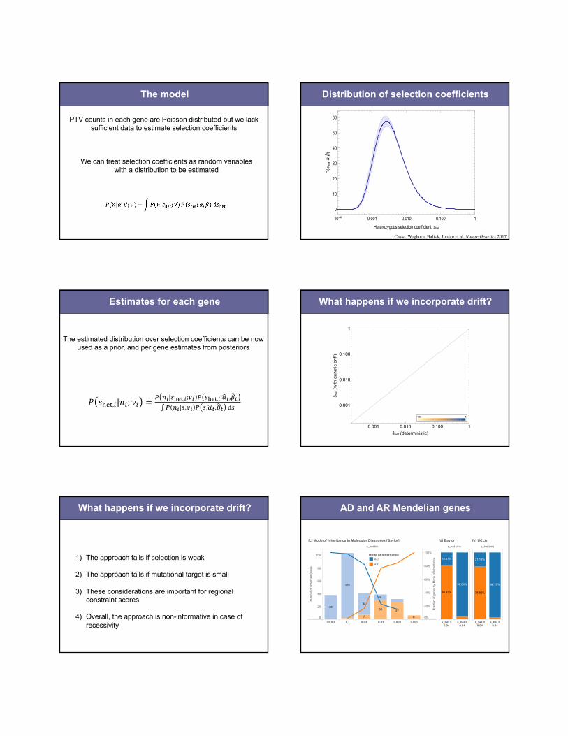
PTV counts in each gene are Poisson distributed but we lacksufficient data to estimate selection coefficients
We can treat selection coefficients as random variables with a distribution to be estimated
Distribution of selection coefficients
10-4 0.001 0.010 0.100 1
0
10
20
30
40
50
60
Heterozygous selection coefficient, shet
P(shet|α,β)
Cassa, Weghorn, Balick, Jordan et al. Nature Genetics 2017
Estimates for each gene
combine the results in a mixture distribution with equal weights. The mean mutation rates in the
three terciles are F^ = 4.6 ∙ 10y~, F= = 1.1 ∙ 10y�, and Fz = 2.6 ∙ 10y�. We estimate (α^, β^) =
(0.057±0.010,0.0052±0.0003), (α=, β=) = (0.046±0.005,0.0087±0.0004), and (αz, βz) =
(0.074±0.005,0.0160±0.0005), with error margins denoting two s.d. from 100 bootstrapping
replicates of the set of ~5,333 genes in each tercile. This error estimate is intended to quantify
the effect of the sampling noise in the data set on the parameter inference while local mutation
rate estimates are assumed fixed. The resulting fitted distributions of counts are shown in
Supplementary Figure 9 together with the corresponding p N , while Figure 1 shows the
inferred V !het; %, ' = IG !het; %^, '^ + IG !het; %=, '= + IG !het; %z, 'z /3. The choice for the
functional form of V !het is motivated by the shape of the empirical distribution of the naïve
estimator W/N (given by a simple inversion of Eq. 3). We also compared the log-likelihood of the
fit to p(N) obtained with this model to that obtained from two other two-parameter distributions,
!het~Gamma and !het~InvGamma, and chose the model with the highest likelihood, which is
!het~IG.
Inference of !het on individual genes From the inferred distributions V !het; %A, 'A in each tercile t of the mutation rate U, we construct
a per-gene estimator of !het for genes in the tercile using the posterior probability given N, which
mitigates the stochasticity of the observed PTV count:
V !"#$,6|N6; W6 =Ü _á|Sàâä,á;gá Ü Sàâä,á;fã,dã
Ü _á|S;gá Ü S;fã,dã dS , (7)
where the denominator is given by Eq. 5. Supplementary Table 1 provides the mean values
derived from these posterior probabilities for each gene. Predicted mode of inheritance in clinical exome cases
We trained a Naïve Bayes classifier to predict the mode of inheritance in a set of solved clinical
exome sequencing cases from Baylor College of Medicine (N=283 cases)22
and UCLA23
(N=176
cases). Using data from UCLA as the training dataset, we are able to cross-predict the mode of
inheritance in separately ascertained Baylor cases with classification accuracy of 88.0%,
sensitivity of 86.1%, specificity of 90.2%, and an AUC of 0.931. Genes that were related to
diagnosis in both clinics (overlapping genes) were removed from the larger Baylor set
(Supplementary Figure 2).
Using a logistic regression based on the full set of cases from Baylor and UCLA, we generated
predictions for all 15,998 genes where there is a !het value (Supplementary Table 4). Mouse knockout comparative analysis
We reviewed mouse knockout enrichments from two datasets: the full set of mouse knockouts
from a neutrally-ascertained mouse knockout screen (N=2,179 genes) generated by the
International Mouse Phenotyping Consortium25
. Genes were classified as ‘Viable’, ‘Sub-Viable’,
or ‘Lethal’ based on the results for the assay. PubMed gene score and enrichment analysis
peer-reviewed) is the author/funder. All rights reserved. No reuse allowed without permission. The copyright holder for this preprint (which was not. http://dx.doi.org/10.1101/075523doi: bioRxiv preprint first posted online Sep. 16, 2016;
The estimated distribution over selection coefficients can be now used as a prior, and per gene estimates from posteriors
What happens if we incorporate drift?(a) (b)
×××××××××××××××
× E[k]
Var[k] /E[k]
0.005 0.010 0.050 0.100 0.500 1
1
2
5
10
Heterozygous selection strength, shet
Foldchangerelativetodeterministiccase
0.001 0.010 0.100 1
0.001
0.010
0.100
1
s�het (deterministic)
s� het(withgeneticdrift)
100 1
Figure 1: Comparison of the deterministic mutation-selection balance model with the model that
includes the effects of genetic drift, in the NFE demography. (a) Fold-change in the coefficient of
variation (squares) and the mean (crosses) of the number of PTV mutations, k, relative to the
deterministic case, obtained from simulations of a realistic demography of the ExAC NFE sample
for different values of heterozygous selection strength shet. (b) Heat map of gene-specific estimates
for all 16,279 tested genes from the NFE sample, showing deterministic (x-axis) and drift-inclusive
(y-axis) shet estimates. Note the double-logarithmic axes in both panels.
12
What happens if we incorporate drift?
1) The approach fails if selection is weak
2) The approach fails if mutational target is small
3) These considerations are important for regional constraint scores
4) Overall, the approach is non-informative in case of recessivity
AD and AR Mendelian genes
Figure 2: Separation of disease genes and clinical cases by mode of inheritance. [a] The distribution of genes associated with exclusively autosomal dominant (AD, N=867) disorders versus autosomal recessive (AR, N=1,482) disorders as annotated by the Clinical Genomics Database (CGD). Logarithmic bins are ordered from greatest to smallest !"#$ values. [b] Overall, AD genes have significantly higher !"#$ values than AR genes [Mann-Whitney p-value 3.14x10-64]. [c] Similarly, in solved Mendelian clinical exome sequencing cases (Baylor)22, !"#$ values can help discriminate between AR and AD disease genes, as annotated by clinical geneticists. [d] A !"#$ value of 0.04 can be used as a simple classification threshold for AD genes with a PPV of 96%. [e] This finding is replicated in a separately ascertained sample from UCLA. Box plots range from 25th-75th percentile values and whiskers include 1.5 times the interquartile range. In a set of 504 clinical exome cases that resulted in a Mendelian diagnosis22, we find a similar enrichment of cases by MOI and selection value (Figure 2[c]). We find that 90.4% of novel, dominant variants are associated with heterozygous fitness loss greater than 0.04 (Figure 2[d]). Among disease variants, a cutoff of !"#$ > 0.04 provides a 96% positive predictive value for discriminating between AD and AR modes of inheritance.
ADDiseaseGenes
ARDiseaseGenes
0.0001
0.0002
0.0005
0.001
0.002
0.005
0.01
0.02
0.05
0.1
0.2
0.5
1
s_he
t
[b] s_het distributions
AD Disease Genes AR Disease Genes
>= 0.3 0.1 0.03 0.01 0.003 0.001 0.0003 >= 0.3 0.1 0.03 0.01 0.003 0.001 0.00030%
2%
4%
6%
8%
10%
12%
Frac
tion
of g
enes
in e
ach
s_he
t bin
(10^
-x)
[a] Mode of Inheritance [Clinical Genomic Database]
s_het bin
>= 0.3 0.1 0.03 0.01 0.003 0.0010
20
40
60
80
100
Num
ber o
f obs
erve
d ge
nes
0%
20%
40%
60%
80%
100%
Frac
tion
of g
enes
by
Mod
e of
Inhe
ritan
ce
102
382730
34
9
7 6
[c] Mode of Inheritance in Molecular Diagnoses [Baylor]
s_het bins
s_het <0.04
s_het >0.04
19.57%
96.04%
80.43%
[d] Baylor
s_het bins
s_het <0.04
s_het >0.04
21.18%
96.70%
78.82%
[e] UCLA
Mode of InheritanceAD
AR
peer-reviewed) is the author/funder. All rights reserved. No reuse allowed without permission. The copyright holder for this preprint (which was not. http://dx.doi.org/10.1101/075523doi: bioRxiv preprint first posted online Sep. 16, 2016;

Age of onset, penetrance and severity
To test the generalizable utility of !"#$ values in prioritizing candidate genes in Mendelian sequencing studies, we compared the overall prevalence of genes with !"#$ > 0.04 to the corresponding fraction in an independently ascertained dataset of new dominant Mendelian diagnoses (Figure 2[e])23. This analysis suggests that restricting to genes with !"#$ > 0.04 would provide a three-fold reduction of candidate variants, given the overall distribution of !"#$ values. Thus, initial effort in clinical cases can be focused on just a few genes for functional validation, familial segregation studies, and patient matching. We summarize the classification accuracy for all possible thresholds (AUC 0.9312) and probabilities for the mode of inheritance in each gene, generated using the full set of clinical sequencing cases (Supplementary Figure 2 and Supplementary Table 2). Beyond mode of inheritance, we find that !"#$ can help predict phenotypic severity, age of onset, penetrance, and the fraction of de novo variants in a set of high-confidence haploinsufficient disease genes (Figure 3). In broader sets of known disease genes, !"#$ estimates significantly correlate with the number of references in OMIM MorbidMap and the number of HGMD disease “DM” variants (Supplementary Figure 3).
Figure 3: Enrichments of !"#$ in known haploinsufficient disease genes of high confidence (ClinGen Project). In (N=127) autosomal genes, we annotate the !"#$ scores of genes associated with each disease category and classification. Higher !"#$ values are associated with increased phenotypic severity (Mann-Whitney p-value 4.87x10-
3), earlier age of onset (p=1.46 x10⁻²), high or unspecified penetrance (p=1.79 x10⁻²), and a larger fraction of de novo variants (p=8x10⁻⁵). Box plots range from 25th-75th percentile values and whiskers include 1.5 times the interquartile range. Gene-specific fitness loss values allow us to plot the distribution of selective effects for different disorders. This provides information about the breadth and severity of selection associated with various disorder groups using both well-established genes (Figure 4[a]) and new findings from Mendelian exome cases (Figure 4[b]). Overall, genes involved in neurologic phenotypes and congenital heart disease appear to be under more intense selection when compared with other disorder groups, tolerated knockouts in a consanguineous cohort, or in all genes (Figure 4[c,d])24. Interestingly, genes recessive for these disorders appear to have only partially
peer-reviewed) is the author/funder. All rights reserved. No reuse allowed without permission. The copyright holder for this preprint (which was not. http://dx.doi.org/10.1101/075523doi: bioRxiv preprint first posted online Sep. 16, 2016;
Concordance with mouse knockout dataviability, while those with the lowest !"#$ estimates are depleted for embryonic lethality [Mann-Whitney p=2.95x10⁻²⁸] (Figure 5[a,b]).
Figure 5: High-throughput screens of gene essentiality in mice and cell assays. [a] Proportion of orthologous mouse knockout genes by phenotype, from a neutrally-ascertained set of genes generated by the International Mouse Phenotyping Consortium (IMCP). Logarithmic bins are ordered from greatest to smallest !"#$ values. [b] ICMP mice are separated into viable (N=1,057), sub-viable (N=211) and lethal knockouts (N=477), and lethal knockouts have significantly higher !"#$ values than viable [Mann-Whitney p-value 2.95x10⁻²⁸]. [c] Cell-essential genes as reported by Wang et al. from genome-wide KBM-7 tumor cell CRISPR assay (N=1,740) have significantly higher !"#$ values [p-value 5.13x10⁻¹⁶] and [d] as do genes that were characterized as essential in a gene trap assay (N= 1,081) [p-value = 4.90x10⁻¹⁸]. In the CRISPR assay, all genes with adjusted p-values < 0.05 and negative assay scores are included, and genes with gene trap scores < 0.4 or lower are included. Box plots range from 25th-75th percentile values and whiskers include 1.5 times the interquartile range.
s_het bin
>= 0.3 0.1 0.03 0.01 0.003 0.001 0.00030%
20%
40%
60%
80%
100%
Per
cent
age
of g
enes
in e
ach
bin,
by
phen
otyp
e
105
215
308
118
283
130144102
55
48
19
57
17
36
71
11
11
7
7
1
[a] Orthologous mouse knockouts by phenotypePhenotype
Lethal Subviable Viable0.0001
0.0002
0.0005
0.001
0.002
0.005
0.01
0.02
0.05
0.1
0.2
0.5
1
s_he
t
[b] Distribution of s_het values
s_het bin
>= 0.3 0.1 0.03 0.01 0.003 0.001 0.00030%
5%
10%
15%
20%
25%
Per
cent
age
of g
enes
cla
ssifi
ed a
s es
sent
ial
458
100
394
292
451
43
2
[c] Cell-Essential by KBM7 CRISPR Assays_het bin
>= 0.3 0.1 0.03 0.01 0.003 0.001 0.00030%
5%
10%
15%
20%
Per
cent
age
of g
enes
cla
ssifi
ed a
s es
sent
ial
175
299
263
236
70
242
[d] Cell-Essential by Yeast Gene Trap Assay
PhenotypeLethal
Subviable
Viable
peer-reviewed) is the author/funder. All rights reserved. No reuse allowed without permission. The copyright holder for this preprint (which was not. http://dx.doi.org/10.1101/075523doi: bioRxiv preprint first posted online Sep. 16, 2016;
RVIS
Petrovski et al. PLOS Genetics 2013
pLI
Lek et al. Nature 2016
probability of being loss-of-function intolerant (pLI) using the expectation-maximization
(EM) algorithm.
The underlying premise of this analysis is to assign genes to one of three natural
categories with respect to sensitivity to loss-of-function variation: null (where protein-
truncating variation – heterozygous or homozygous - is completely tolerated by natural
selection), recessive (where heterozygous PTVs are tolerated but homozygous PTVs
are not), and haploinsufficient (where heterozygous PTVs are not tolerated). We assume
tolerant (null) genes would have the expected amount of truncating variation and then
took the empirical mean observed/expected rate of truncating variation for recessive
disease genes (0.463) and severe haploinsufficient genes (0.089) to represent the
average outcome of the homozygous and heterozygous intolerant scenarios
respectively. These values (1.0, 0.463, 0.089) are then used as a three-state model to
which we fit the observed/expected truncating variant rate of each gene via the following
analysis.
Let !! represent the proportion of all genes that fall into one of the three proposed
categories: null, recessive, and haploinsufficient (!! ∈ ! !"##,!"#,!" ).
Let λNull, λRec, and λHI denote the expected amount of loss-of-function depletion in each of
the three categories. Based on the observed depletion of protein-truncating variation in
the Blekhman autosomal recessive and ClinGen dosage sensitivity gene sets
(Supplementary Information Table 12), we use:
λNull = 1
λRec = 0.463
λHI = 0.089
For each gene i, we model the observed data (PTV counts) as a function of the
unobserved class labels (Zi) as follows:
!! !|!!!~!!"#$%&'(")(!!"## ,!!"# ,!!")
!"#! !|!!! = !!~!!"#$(!!!)
WWW.NATURE.COM/ NATURE | 33
Here, PTVi represents the observed number of PTVs in gene i and N is sample size,
such that !!! is the expected number of loss-of-function variants in a gene belonging to
class c in the ExAC data. Our goal is to find the maximum-likelihood estimate (MLE) for
π (the mixing weights of the three gene classes), and to use this estimate to obtain an
Empirical Bayes maximum a posteriori (MAP) estimate for Zi – the probability of gene
assignment to each category – for all genes i=1…M.
We use an expectation-maximization (EM) algorithm to find the MLE for π and Zi,
treating π as the parameters and the Zi as the latent variables. We initialize the EM
algorithm by setting !! = (1 3 , 1 3 , 1 3).
In the E-step, we evaluate the distribution of the latent variables (Zi) given the values of
the parameters (π) from the previous iteration. The E-step is
! !! = !!|!!! ,!"#! = !"#$ !"#! ! !!!!)!!!"#$ !"#! ! !!!!)!!!
,
where !"#$ denotes the Poisson likelihood. In the M-step, we update the parameters π
with a new expectation taken under the distribution of the latent variables (Zi) computed
in the M step. The update is
!!!"# ∶= ! ! !! = !!|!!"#!,!!!"# /!"#$#%!
We repeat these steps until the convergence criteria are met (!!" changes by less than
0.001 from one iteration to the next).
When the EM has converged, the final mixing weights (π) are used to determine each
gene’s probability (! !! = !! !! ,!"#!)) of belonging to each of the categories (null,
recessive, haploinsufficient).
WWW.NATURE.COM/ NATURE | 34
De novo mutations in ASD
Kosmicki et al. Nature Genetics 2017
Heritability enrichment
ANALYSIS NATURE GENETICS
However, despite extremely large CVE and LFVE, this class of vari-ants had a smaller LFVE/CVE ratio than that of non-synonymous variants inside genes predicted to be under weak selection (Fig. 5), a surprising result that appears to suggest a smaller ∣ ∣sdn (Fig. 6b) despite the extremely large value of π del. We performed additional forward simulations to show that a larger ∣ ∣sdn does not produce larger LFVE/CVE ratios for annotations with extremely large values of π del, for which the ratio between the proportion of low-frequency
variants that are deleterious and the proportion of common variants that are deleterious is reduced to 1 (Supplementary Fig. 12).
Although our focus is primarily on low-frequency variants (0.5%≤ MAF < 5%), we also used our forward simulation frame-work to draw inferences about rare variant (MAF < 0.5%) architec-tures of non-coding functional annotations, based on LFVE and CVE estimates from UK Biobank (Fig. 4a). Specifically, we com-pared the mean squared per-allele effect size of rare causal vari-ants in annotations mimicking functional non-coding variants and non-synonymous variants, respectively. We inferred disproportion-ate causal effects of rare variants in annotations under very strong selection (sdn = − 0.003, similar to non-synonymous variants13), with mean squared causal effect sizes 11× , 26× , and 60× larger than annotations with sdn = − 0.0006, sdn = − 0.0003, and sdn = − 0.0002, respectively (Fig. 6d and Supplementary Table 12; similar results for different choices of π , Supplementary Fig. 13). These results indicate that an annotation with large CVE needs to have even larger LFVE (for example, LFVE/CVE ratio ≥ 2× , corresponding to sdn ≤ − 0.0006; Fig. 6b) in order to harbor rare causal variants with substantial mean squared effect sizes (for example, only an order of magnitude smaller than rare causal non-synonymous variants; Fig. 6d). Unfortunately, most of the non-brain CTS annotations that we analyzed do not achieve this ratio (Fig. 4a), motivating further work on more precise non-coding annotations (see Discussion).
DiscussionIn this study, we partitioned the heritability of both low-frequency and common variants in 40 UK Biobank traits across numerous functional annotations, employing an extension of stratified LD score regression5,23 to low-frequency and common variants, which produces robust (unbiased or slightly conservative) results. Meta-analyzing functional enrichments across 27 independent traits, we highlighted the critical impact of low-frequency non-synonymous variants (17.3% of hlf
2, LFVE = 38.2× ) compared to common non-synonymous variants (2.1% of hc
2, CVE = 7.7× ). Other annotations previously linked to negative selection, including non-synonymous variants with high PolyPhen-2 scores29, non-synonymous variants in genes under strong selection31, and LD-related annotations23, were also significantly more enriched for hlf
2 compared to hc2. Finally,
at the trait level, we observed that CTS annotations6,8 also domi-nate the low-frequency architecture and that significant CVE tend
2 5 10 20 50
2
5
10
20
50
CVE
LFV
E
a
Brain CTS annotationNon-brain CTS annotationNon-synonymousCodingAge first birth (germinal matrix)Neuroticism (prefrontal cortex)
0.0 0.2 0.4 0.6 0.8 1.0
0.0
0.2
0.4
0.6
0.8
1.0
Pro
port
ion
of h
lf2
Proportion of hc2
b
1x
2x
3x
5x
Fig. 4 | Low-frequency and common variant architectures of CTS annotations. a,b, For 637 trait–annotation pairs with conditionally statistically significant common variant enrichment, we report LFVE versus CVE (log scale) (a) and proportion of hc
2 versus proportion of hlf2 explained (b). The dashed black line
in a represents the regression slope for 25 critical CTS annotations for independent traits (see main text). Brain-specific annotations are denoted in blue. Two trait-H3K4me3 annotation pairs with LFVE significantly larger than CVE are denoted in dark blue (see main text); error bars represent 95% CI. The two arrows in b denote All autoimmune diseases (H3K4me1 in regulatory T-cells; left arrow) and Monocyte count (H3K4me1 in primary monocytes; right arrow) (see main text). Results for coding and non-synonymous annotations (meta-analysis across 27 independent traits) are denoted in red; error bars represent 95% CI. Numerical results are reported in Supplementary Table 10.
1 2 5 10 20 50 100
1
2
5
10
20
50
100
CVE
LFV
E
1x
2x
3x
5x
shet bin 1 (strongest selection)shet bin 2shet bin 3shet bins 4+5 (weakest selection)
(0.02% / 0.04%)(0.03% / 0.06%)(0.04% / 0.08%)(0.11% / 0.17%)
Proportion of variants (common / low-freq)
Fig. 5 | Low-frequency and common variant enrichments for non-synonymous variants vary with the strength of selection on the underlying genes. We report LFVE versus CVE (log scale) for non-synonymous variants in five bins of shet (see main text), meta-analyzed across 27 independent UK Biobank traits; bins 4!+ !5 are merged for visualization purposes. Numbers in the legend represent the proportion of common/low-frequency variants inside the annotation, respectively. The solid line represents LFVE!= !CVE; dashed lines represent LFVE!= !constant multiples of CVE. Error bars represent 95% CI. Numerical results for each bin are reported in Supplementary Table 11.
NATURE GENETICS | VOL 50 | NOVEMBER 2018 | 1600–1607 | www.nature.com/naturegenetics1604
Gazal et al. Nature Genetics 2018