1

Reinhard Blutner

Musical Forces and Quantum Probabilities

Emeritus member of ILLC, Universiteit van Amsterdam, Amsterdam, The Netherlands. email: blutner@contact.uva.nl

Abstract: In cognitive music theory, musical forces arise in connection with tonal attraction. How well does a given pitch fit into a tonal scale or tonal key, let it be a major or minor key? A similar question can be asked regarding musical sequences and tonal progression: What the level of resolution is felt when hearing a probe tone following a certain chord in a two-step serial sequence? After giving a concise review of the empirical findings concerning both types of attractions, I will outline several models for explaining the findings. The basic shortcoming of these models is that they cannot simultaneously describe both attraction types.

To overcome the failings of the earlier models, both methodologically and empirically, I propose a new kind of model relying on insights of the new research field of quantum cognition. I will argue that the quantum approach integrates the insights from both group theory and quantum probability theory. In this model, tones are described as vector states ("wave functions") of a Hilbert space way, and the twelve tones can be seen as forming a cyclic group. The phenomenon of attraction is described as the projection of the context (described as a vector state) into a vector state describing the probe tone. I will further demonstrate that a description of the phenomenological forces behind both attraction types is possible in terms of quantum probabilities.

The quantum theoretic analysis of forces is quite different from the phenomenological treatment of our naïve understanding of physics. In modern quantum field theory, physical forces are seen as derived from local phase shifts in an underlying grid of wave functions. Surprisingly, when considering musical movements in a theory of tonal music this idea makes equally sense. The rationale behind the phase shifts are regular micro-forces that correspond to the two types of attractions. These micro-forces are at a different level than the phenomenological forces discussed in folk theories of music. I will demonstrate that the micro-forces can be interpreted within a markedness theory of tonal music. The unmarked case corresponds to the force-free case; musical gauge forces are the rationale behind marked attraction behavior. Keywords: Quantum cognition; lattice gauge theory; tonal attraction; computational music theory; generative music theory; markedness theory, interval cycles; musical expectation; affective meaning.

1. Introduction The application of physical metaphors is quite common in theories of music. The basic assumption seems to be that our experience of musical motion is in terms of our experience of physical motion and their underlying forces. For example, Schönberg speaks of different forces when he explains the direction of musical forces in cadences where the tonic attracts the dominant (Schönberg, 1911/1978, p. 58). In addition, Larson (1997-98, 2004; Larson, 2012) proposed three musical forces that generate melodic completions. These forces are called ‘gravity’, ‘inertia’, and ‘magnetism’, respectively. These forces should be seen as conceptual metaphors in the sense of Lakoff and Johnson (1980). They structure our musical thinking per analogy with falling, inert and attracting physical bodies. Physical forces are represented in our naïve (common sense) physics or folk physics.

In contrast to Larson, Mazzola (1990, 2002) provides a quite different analogy between music theory and modern (non-folk) physics. Modern foundational physics describes the forces that cause the interaction between elementary particles. In these theories, forces are seen as caused by the "exchange" of certain particles. The physical forces are basically connected with certain symmetries of the physical micro-world. Mazzola was the first who saw the analogy between physics and music in connection with the existence of symmetries ‒ in music especially for the domain of modulation:

2

Als Transformationskraft wirkt das Modulationsmittel der Modulation. Die Lokalisierung der „Teilchen“ geschieht durch die Kadenz der Modulation. Diese Sprechweise ist der Musikwissenschaft nicht fremd: Schönberg, Uhde und viele andere sprechen in einem vagen Sinne physikalistisch von „Kräften“ zwischen musikalischen Strukturen, wenn es darum geht, Veränderungen verständlich darzustellen. (Mazzola 1990, p. 200)

Even when we will not study the domain of modulation in the present study, Mazzola's insights are of highest importance for the present paper. As the central problem of the present paper, we will investigate the question of tonal attraction. The term “tonal attraction” refers to the idea that melodic or voice-leading pitches tend toward other pitches in greater or lesser degrees. The present conception sees a close relationship between the phenomenon of tonal attraction and the existence of tonal forces.

I will start with an important distinction. Let us assume that there are tonal forces that determine the center(s) of a series of tones or chords – call it the "static forces" and that there are forces that affect tonal progression or chord progression (dynamics) – call it the "dynamic forces". How well does a given pitch fit into a tonal scale or tonal key, either being a major or minor key? This is a question of the first type concerning the tonal centers. A question of the second, dynamic type could ask, for example, for the level of resolution a subject feels when she hears a probe tone following a certain chord in a two-step serial sequence.

In an celebrated study by Krumhansl and Kessler (1982) the first type of tonal attraction was investigated. In this study, listeners were asked to rate how well each note of the chromatic octave fitted with a preceding context, which consisted of short musical sequences in major or minor keys. The results of this experiment clearly show a kind of hierarchy: the tonic pitch received the highest rating, followed by the pitches completing the tonic triad (third and fifth), followed by the remaining scale degrees, and finally the chromatic, non-scale tones. This finding plays an essential role in Lerdahl's and Jackendoff's generative theory of tonal music (Lerdahl & Jackendoff, 1983) and is one of the main pillars of the structural approach in music theory. A related approach is due to Bharucha (1996). The second type of attraction was investigated by Krumhansl (1990, 1995), Lake (1987), Bharucha (1996), Lerdahl (1996), Larson (2004); Larson (2012), and in a recent study of Woolhouse (2009), following earlier research of Brown, Butler, and Jones (1994).

Both types of tonal attraction have not only initiated an enormous number of empirical studies but also a series of different models that are based on static and dynamic forces. It goes without saying that I can discuss here only a few of these models. Most of these models are close in inspiration to Larson (2012). All models explicitly or implicitly consider the term "musical forces" as a metaphoric term and build a phenomenological model on this basis. That means these models aim to describe the phenomena of musical attraction without developing a deeper foundational perspective that can explain the phenomena. The work of Mazzola is an important exception to this widely shared methodology. His theory sees the whole conception of "musical force" as directly rooted in the basic symmetry principles of tonal music. To distinguish the phenomenological forces from the forces based on fundamental symmetries, I will call the latter "micro-forces". One of the aims of this article is to bring together the two quite different perspectives of considering musical forces.

In an earlier study (Blutner, 2015), I have discussed the static site of tonal attraction. The study has been concentrated on modelling the tonal centres of a tonal scale (or sequence of chords). To overcome the shortcomings of earlier models, both methodologically and empirically, the proposed model relies on insights of the new research field of quantum cognition. The model integrates the insights from group theory (symmetries and invariances) and quantum probability theory (defining a

3

measure for attraction). In the present article, this approach is extended to include the dynamic site of musical attraction. It is important that the present model can integrate both attraction types. Thus, it overcomes a basic shortcoming of all earlier models.

In the following section, I will compare the concepts of physical and musical forces and I will explain why the modern concept of forces as developed in quantum field theory makes sense for cognitive music theory. In Section 3, I will review some basic empirical findings about tonal attraction, concerning both the static and the dynamic aspects. Section 4 discusses several phenomenological models of tonal attraction, which in fact are folk theories of tonal forces. Section 5 develops a first and very simple quantum model of tonal attraction. It extends my earlier study (Blutner, 2015) and it exploits the symmetry principle of transposition invariance. Section 6 sees tonal force as causing a phase shift of the underlying wave function. Gauge theory is applied for exploiting the heart of quantum field theory in music: relating symmetries and gauge fields. I introduce a gauge field based on the Harmonic oscillator. This solves the problem of arbitrary phase parameters. Further, I will argue for deep gauge where the quantum field is iteratively gauged through an evolutionary mechanism of deep learning, similar to bidirectional optimality theory in cognitive linguistics.

In Section 7, the advantages of the quantum approach are explained and some general conclusions are drawn. I finally argue that the present model achieves a profounder understanding of the cognitive nature of tonal music, especially concerning the nature of musical expectations (Leonhard Meyer) and its role for a better understanding of the affective meaning of music.

In the Appendix, I introduce the basic mathematical concepts that are needed for an understanding of quantum cognition. It goes without mentioning that no background in physics is required to understand this concise introduction. In addition, little or no reference to physics will be made during the main part of this article.

2. Physical and musical forces In classical physics, a force is seen as the cause of any change of the motion of an object. A force has a magnitude and direction making it a vector. According to Newton's second law the force acting upon an object is equal to the rate at which its momentum (= mass times velocity of the object) changes with time. Notably, our intuitive understanding of physical forces is not exactly the same as Newton's physical understanding. This is especially visible in connection with Newton's first law. It states that physical objects continue to move in a state of constant velocity unless acted upon by an external force. This conflicts with our everyday experience assuming that objects move with constant velocity only when a constant force is applied (due to the hidden role of friction or turbulences). Aristotle, to be sure, was much closer to folk physics than Galilei, who was the first who constructed experiments to disprove Aristotle's theory of movement.

Within the last 100 years, the distance between theoretical physics and folk physics has increased even more. In modern particle physics, forces and the acceleration of particles are explained as a mathematical by-product of exchange of momentum-carrying tiny particles (so-called gauge bosons). With the development of quantum field theory and general relativity, it was realized that force is a redundant concept arising from conservation of momentum (4-momentum in relativity and momentum of virtual particles in quantum electrodynamics). The conservation of momentum can be directly derived from the homogeneity or symmetry of space and so is usually considered more fundamental than the concept of a force. Hence, the modern understanding of physical forces

4

sharply contrasts with our folk physical understanding, which is sometimes taken as a sign of progress in science (Weinberg, 1992).1

As mentioned in the introduction, there are two quite different concepts of musical forces in cognitive music theory. According to the metaphoric conception, musical forces are seen in analogy to physical forces in folk physics as a means to describe musical movements. In contrast, there is the interactional conception, which shares correspondences with modern physics. It considers musical micro-forces as an emergent (and redundant) concept that arises from the existence of symmetries and invariance principles in tonal music. This is in line with the framework of Mazzola (1990, 2002) who sees the modern idea of forces – as founded in the interaction and exchange of "particles" – as directly applicable for modelling the process of modulation and the phenomenological forces that act in this process.

In the present article, I will not see a clashing conflict between the two conceptions of musical forces. Instead, I will consider the two concepts as complementary. That means both conceptions are useful but they correspond to different perspectives. The metaphoric conception seeks to provide a high-level description of the basic traits of musical movement. In contrast, the interactional conception applies at a deeper, more foundational level. In a certain sense, it relates much closer to the neuronal hardware that underlies music cognition. Even when the present state of the art does not allow to draw a direct connection with the neuronal underpinning of all psychological processes, there are hints that particularly spiking network can profit from dynamic descriptions that are borrowed from quantum mechanics (Acacio de Barros & Suppes, 2009).

Here is an informal outline of the basic idea of the interactional conception. According to Penrose (2004), all physical interactions are governed by "gauge connections" which, technically, depend crucially on spaces having exact symmetries (p. 289). From the perspective of quantum physics, there is an absolute need of an invariance of the theory under a local phase transformation. The point is that any physical system is described by a wave function. However, such wave functions are not directly observable. Only probabilities can be observed. Hence, an arbitrary phase factor should not change the observation of probabilities of measurements. Generally, the underlying principle is called gauge invariance where the underlying symmetry group is the group of local phase transformations U(1) or an extension of this group.2 Appendix A4 explains the principle of gauge invariance in more detail.

1 Modern physics accepts exactly four fundamental forces. These are besides electromagnetic and

gravitational forces, strong and weak nuclear forces. All other forces (such as friction, tension and elastic forces) can be derived from the four fundamental forces. The four fundamental forces are more accurately considered as "fundamental interactions". The development of fundamental theories for forces proceeded along the lines of unification of disparate ideas. The modern story starts with Newton who unified the force responsible for objects falling at the surface of the Earth with the force responsible for the orbits of celestial mechanics in his universal theory of gravitation. Faraday and Maxwell demonstrated that electric and magnetic forces were unified through one consistent theory of electromagnetism. In the last century, the development of quantum mechanics led to a modern understanding that the electromagnetic and the two nuclear forces are manifestations of matter interacting by exchanging virtual particles (so-called gauge bosons). This is the "standard model" of particle physics, and it posits a similarity between all forces (except the gravitational force). The complete formulation of the standard model includes the recently observed Higgs mechanism.

2 As an example, the description of electrons as formulated by the Dirac equation can be considered. In this case, the multiplication of the wave function with a local phase factor eiϕ(x,t) introduces an additional term in the transformed Dirac equations which destroys the symmetry. The crucial idea is to compensate the destroying term by an additional term modifying the original electromagnetic potential. This term is seen as

5

In quantum cognition, tones are consider as the simplest states of the musical system and as such, they can be described by wave functions. As a consequence, crucial principles of tonal music can be formulated with the help of the mathematical mechanisms of quantum physics (Blutner, 2015). Not surprisingly, it is tempting to use the mechanism of gauge invariance for introducing musical forces. Changes of states (movements) are described by the Schrödinger equation in classical quantum mechanics. Hence, this equation is the starting point for our discussion of gauge invariance and symmetry. In Section 6 we will see that this idea makes sense already in the simple case of analysing phenomena of tonal attraction.

3. The phenomenon of tonal attraction According to Philip Ball the core of any scientific explanation of music is an understanding of how and why it affects us (Ball, 2010). Ball considers affective meaning as an important level of musical representation, having in mind the form of meaning which Meyer (1956) sees as embodied meaning − referring to the significance a musical event can have for a listener in terms of its own structure and in interaction with the listener's musical expectations. Meyer (1956) pointed out that the principal emotional content of music arises through the composer’s arranging of expectations. The secret to composing a likeable song is to balance predictability and surprise. Because most music has a beat and is based on repetition, we know when the next musical event is likely to happen, but we do not always know what it will be. Our brains are working to predict what will come next. The skillful composer rewards our expectations often enough to keep us interested, but violates those expectations the rest of the time in interesting ways. The ability to model our predictions about what could be the next pitch or chord in a given tonal context is an important step in modelling affective meaning. However, it is not the exact prediction of a pitch or chord that matters but its characterization as consonant/dissonant (cf. Blutner, 2015).

At present, there is no common agreement about the exact content of the idea of affective meaning. Is it directly related to our expectancies of consonance and dissonance, as Meyer seems to suggest? Alternatively, do we need other concepts in order to grasp its content? What about the terms stability and tension that play an important role in cognitive music theory (Lerdahl & Jackendoff, 1983)? To be sure, the two concepts are closely related: stability can be seen as a reduction of tension. Hence, stable pitches are more probable than instable ones, and dissonant chords exhibit more tension than consonant ones. For that reason, we can expect a high positive correlation between measures of affective meaning based on expectancies of consonance/disson-ance and measures based on stability/tension. In a recent study Lerdahl & Krumhansl (2007) investigated how to predict the rise and fall in tension in the course of listening to a tonal piece. In effect,

describing an interaction of the original electromagnetic field with a gauge field. Obviously, this idea realizes a new dynamical principle coupling the gauge field with the electromagnetic field of the electron. There is a natural interpretation of the gauge field: it describes the interaction of a photon with the electron. In other words, the exchange of a photon is realizing a new force found by the idea of a gauge transformation. A more complex case is the standard model of particle physics. The model is formulated as a non-Abelian gauge theory with the symmetry group U(1)×SU(2)×SU(3). It has twelve gauge bosons: the photon, three weak bosons and eight gluons. Between quantum electrodynamics and the full complexity of particle physics, there are symmetry groups such as SU(2) which correspond to the Schrödinger-Pauli equation and U(1)×SU(2) for the Schrödinger-Pauli equation including a Higgs field to give spin-1/2 dyons their masses.

6

this research suggests the view that the judged values of tension can be described by a combination of both types of tonal attraction together with assumption about tonal consonance and dissonance.

From the point of view of musical analysis is it is important to have a whole battery of different measures besides tonal attraction. Stability, tension, and relaxation are among the interesting measure functions that deserve our attention. An important task is the possibility to derive these functions from more basic and possibly more abstract functions. The situation is alike the situation in linguistic semantics (e.g., Katz, 1972; Katz & Fodor, 1963): there are many complementary concepts such as synonymy, contrast, entailment, semantic equivalence, polysemy, etc. that can be derived from a basically theoretical (non-observable) abstract meaning function. The present study discusses whether the idea of musical forces is substantial for identifying the underlying base functions. The investigation of the two attraction types together with measures about consonance/dissonance can help to identify the underlying resources.

For the following, we make use of the notion of a tonal pitch system. A tonal pitch system consists of a number of pitches where pitches are sounds defined by a certain fundamental frequency. In this paper, we assume twelve pitch classes, also called tones3, and we will use a numeric notation to define the twelve tones of the system ('scale degrees' i, with i running from 0 to 11), in ascending order:

(1) 0 = C, 1 = C♯, 2 = D, 3 = D♯, 4 = E, 5 = F, 6 = F♯, 7 = G, 8 = G♯, 9 = A, 10 = B♭, 11 = B The general phenomenon of tonal attraction can be investigated in different ways. For example, in the probe-tone technique, the listener is confronted with a tonal context and a probe tone or probe chord and the listener has to rate how well the probe element fits into the tonal context. Given a chord of C major as context, how well does the tone X (an element of the diatonic C-major scale or the whole chromatic scale) fit to this chord? In this way, attraction of the first type (static attraction) can be investigated. I mentioned already the pioneering study Krumhansl and Kessler (1982) for the first type of tonal attraction. Using standard psychological techniques, a static attraction profile can be constructed. The probe-tone technique can also be taken to investigate attraction of the second type (dynamic attraction) – considering the temporal progression of musical pieces. How well does the probe tone X resolve a tonal chord or sequence of chords? How plausible (on a scale from 1 to 7) is it that this probe tone immediately follows the cue chord? An interesting application of the attraction judgement task in the dynamic case was carried out by Brown et al. (1994) and in a recent study of Woolhouse (2009). In his book, Larson (2012) reports on particular listener judgment experiments. In these experiments, the strength of melodic pattern completions was tested. For example, subjects were asked to rate a given series of three-note pattern on a scale of 1 to 7 (7 being highest) based on how strongly they felt the second note "lead" to the third note.

Another possibility to investigate tonal attraction is by means of melodic production tasks. These tasks investigate the generation of pitches that continue and possibly complete a given piece of pitches (or chords) in a "melodic way". For example, Cuddy and colleagues (Cuddy & Lunney, 1995; Thompson, Cuddy, & Plaus, 1997) investigated the behaviour of musically trained and untrained persons in a melody completion task. In the 1995 study ratings of continuation tones presented after the implicative intervals were investigated whereas in the 1997 study a melody production task was

3 Tones can be seen as equivalent classes of pitches. Two pitches with fundamental frequencies f1 ≥ f2 are

equivalent if f1 / f2 is a natural number (i.e., the two pitches are equal or have a distance of one or more octaves). Hence, the concept of tones as equivalence classes of pitches abstracts from the octave level.

7

investigated. In detail, the subjects were asked to continue a melody the first two tones of it were presented in 8 trials for each of 8 initial intervals. For each melody, the note immediately following the initial interval was analysed.

Besides judgement and production tasks, there are methods that enable real-time judgments of musical parameters such as tension and other proxies for musical affect. Experiments by Vines, Nuzzo, and Levitin (2005) and Lerdahl and Krumhansl (2007) use continuous tension judgment in order to assess a participant’s real-time experience of a musical piece. Participants indicate the ongoing tension they feel while listening to a musical piece by adjusting a continuous response interface, for instance a moveable slider.

The application of standard psychological techniques to collect empirical data is not the only instrument available. Another instrument is collecting corpus data, which became a rather popular method within the last years. For example, the Kostka-Payne corpus consists of 46 excerpts from the common-practice repertoire, taken from the workbook accompanying the author's textbook (Kostka & Payne, 1995). The relevant data represent pitch-classes relative to keys. As an example, the tonic pitch occurs in 74.8% of segments in major keys. Scale degree 4, by contrast, occurs in only 9.6% of segments. The profiles reflect conventional musical wisdom, much as we would expect. Not unexpectedly, there is a high correlation between the Krumhansl and Kessler attraction data and the Kostka-Payne profiles (cf. Temperley, 2007). Another instance for corpus studies was presented by Huron (2006). Huron's data (Huron 2006: 251) consist of the frequencies of various chord progressions in a sample of baroque music.

In the following two subsections we give a representative overview about the basic findings representing the statics and dynamics of tonal attraction. Our discussion will be concentrated on probe items consisting on single tones. For a discussion of chordal data including the Huron data, I refer to my earlier publication (Blutner 2015).

3.1 The statics of tonal attraction Now we will discuss the Krumhansl and Kessler (1982) study investigating the first type of tonal attraction. As mentioned already, in this study a probe tone technique was applied, and the listeners were asked to rate how well each note of the chromatic octave fitted with a preceding context. The results of this study are shown in Fig. 1 for contexts establishing major keys. The figure also presents related corpus data of Kostka & Payne (1995), which were appropriately scaled in order to allow a direct comparison. Both the results of this experiment and the corpus data clearly show a kind of hierarchy: the tonic pitch (level A) received the highest rating, followed by the pitches completing the tonic triad (third and fifth; = levels B & C). This is followed by the remaining scale degrees (level D). Finally, we find the chromatic, non-scale tones (level E).

8

C D♭ D E♭ E F G♭ G A♭ A B B♭ (Probe Tones)

Fig. 1: Distribution marked by ∙: data of Krumhansl & Kessler (1982) for the key C major; distribution marked by : corpus data of Kostka & Payne (1995). A linear transformation was applied in order to make both kinds of data compatible. Regarding the function of the tonic hierarchy in tonal music, we refer to the insights of Philip Ball:

Although it is normally applied only to Western music, the word 'tonal' is appropriate for any music that recognizes a hierarchy that privileges notes to different degrees. That's true of the music of most cultures. In Indian music, the Sa note of a that scale functions as a tonic. It's not really known whether the modes of ancient Greece were really scales with a tonic centre, but it seems likely that each mode had at least a 'special' note the mese, that, by occurring most often in melodies, functioned perceptually as a tonic. This differentiation of notes is a cognitive crutch: it helps us interpret and remember a tune. The notes higher in a hierarchy offer landmarks that anchor the melody, so that we don't just hear it as a string of so many equivalent notes. Music theorists say that notes higher in this hierarchy are more stable, by which they mean that they seem less likely to move off somewhere else. Because it is the most stable of all, the tonic is where melodies come to rest. (Ball 2010: 95)

As we have seen, the probe tone techniques used in the experiments by Krumhansl, Kessler and others ask listeners directly to judge how well a single probe tone or chord fits an established context, and the relevant data collected by this technique represent the static site of tonal attraction. However, the finding that some tones are more stable than others invites some speculation about the dynamics of attraction: When considering sequences of pitches, "a melody is then like a stream of water that seeks the low ground" (Ball 2010: 95). Hence, modifying a picture of Ball (2010), there seem to be forces that are directed toward the tones of the tonic triad (see Fig. 2).

A

B C

D

E

9

Fig. 2: Hypothetical melodic forces (modified from Ball, 2010). The tones of the tonic triad are

encircled In the next subsection, I will describe the basic findings of the dynamically-inspired experiments in a model-independent way.

3.2 The dynamics of tonal attraction Lerdahl makes a careful distinction between tonal hierarchies and event hierarchies. The latter are "part of the structure that listeners infer from temporal musical sequences" (Lerdahl 1988: 316). Data that concern "chord progression" should be explained in terms of such event hierarchies. The classical tonal attraction experiments can be modified by asking listeners to rate the degree to which a tone or chord is expected in that context ‒ following a sequence of pitches or chords as the subsequent element. Some of these studies (Cuddy & Lunney, 1995; Krumhansl, 1995; Schellenberg, 1996; Thompson et al., 1997) used the probe-tone technique to investigate the tone-to-tone expectancies for continuations of melodies. These studies are important to test the dynamic predictions of models of melodic expectancy, such as Narmour's implication realization model (Narmour, 1991, 1992).

3.2.1 Woolhouse (2009) The first experiment I will discuss concerns recent investigations by Woolhouse (2009). His probe-tone experiment limits analysis to only the first new element after the presentation of the context chord. In the original experiments, five different context chords are considered: major triad {C, E, G},

minor triad {C, E♭, G}, dominant seventh {C, E, G, B♭}, French sixth {C, E, G♭, B♭}, or half-diminished

seventh {C, E♭, G♭, B♭}. Probe tones are all twelve tones of the chromatic scale. Both the context chord and the probe tone each lasted two seconds. There was no temporal gap between context chord and probe tone. The subjects had to decide (on a 7 point Likert scale) "the level of attraction and/or resolution they felt from the chord to the probe tone: seven for a high level of attraction, one for a low level of attraction". For brevity, we will be concentrated on the results triggered by the major triad and the dominant seventh. The data are shown in Fig. 3. In contrast to the static case presented in Fig. 1, it is remarkable to note that the chromatic pitches of the key of C major did not all receive the lowest ratings. Further, the pitches of the tonic triad did not all receive considerably

10

high ratings. The most important fact is that F was rated significantly higher than any other pitch. C gets the lowest value for the C-major chord and an intermediate value for the dominant seventh. Even E and G get rather low values.

C D♭ D E♭ E F G♭ G A♭ A B B♭ (Probe Tones)

Fig. 3: Distribution marked by ∙: data of Woolhouse (2009) for the C major chord; distribution marked by : Woolhouse's data for the dominant seventh.

The main difference between the two contexts is that for the dominant seventh the attraction values for pitch C and pitch B are significantly higher than for the C-major chord. This is an immediate consequence of the pitch B♭ in the dominant seventh chord.

3.2.2 Piston (1979) and Huron (2006) It is possible to collect tonal attraction values for all chord pairs of a given region (key). The first chord represents the context and the second chord represents the probe which has to be judged how well it can be seen as the consequent chord in a series of chord progression. Piston (1979) was the first who came with (semi-empirical) table of expectation in chord progression. Piston’s table consists of statements like “IV is followed by V, sometimes I or II, less often III or VI.” Woolhouse (2010) quantified such statements by identifying four levels of chord-progression frequency: “is followed by” was rated 4, “sometimes” was rated 3, “less often” was rated 2, and a progression not mentioned was rated 1. Fig. 3 (top) shows a stacked chart with scaled data reflecting Piston's table.

11

Fig. 4: Stacked chart reflecting Piston's table of chord progression (top) compared with data from

Huron (2006: 251) based on a sample of baroque music (bottom).

Recently, Huron (2006) has presented data based on corpus studies (Huron 2006: 251). These data consist of the frequencies of various chord progressions in a sample of baroque music. From these data the probabilities of a chord given some antecedent chord are derived (i.e., we consider the conditioned probabilities P(probe chord/antecedent chord)). The stacked chart presented on the bottom part of Fig. 3 shows these conditioned probabilities. Note that the conditioned probabilities for each chord sum up to 1 in the diagram. The broader the considered "second chord strip" for a given "first chord", the higher the probability of the considered probe chord. Even a shallow comparison between the Piston table and the Huron data shows capital discrepancies. The correlation value between the two data sets is considerably low (r = 0.21). Nevertheless, both the Piston table and Huron's data reflect basic pattern of chordal developments, for instance, that the dominant (V) is preferably leads to the tonic chord (I) and that the subdominant (IV) is preferably followed by the dominant (V), even when the Huron data are more trustworthy concerning the quantitative traits.

3.2.3 Cuddy and colleagues Next, I will consider data that more directly reflect the melodic developments. As mentioned already Cuddy and colleagues (Cuddy & Lunney, 1995; Thompson et al., 1997) used the probe-tone technique to test the dynamic predictions of models of melodic expectancy. The results of both investigations are compatible. The present summary of the results will be based on the 1997

12

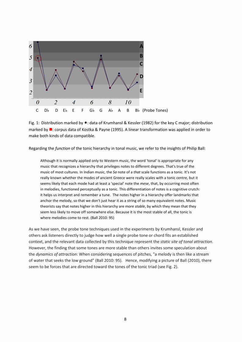
production study. It investigated five (preferential) principles, which partly are based on Narmour's Gestalt-like conception:4

Registral direction states that small intervals (≤ 5 semitones) imply continuation in the same registral direction (e.g., up–up), whereas large intervals (≥ 7 semitones) imply a change in registral direction (e.g., up–down; up–lateral). Intervallic difference states that small intervals imply a subsequent interval that is similar in size (i.e., the same size ± 2 semitones if registral direction changes, the same size ± 3 semitones if registral direction stays the same), whereas large intervals imply an interval that is relatively smaller in size (at least 3 semitones smaller if registral direction changes and at least 4 semitones smaller if registral direction stays the same. Note that a “smaller” interval is not always a “small” interval). Registral return occurs when an interval moves to a third note that is identical to or near (±2 semitones) the first note of that interval. Proximity is defined as less than or equal to 5 semitones between any 2 notes. Finally, closure occurs when there is a change in registral direction (e.g., up–down), movement to a smaller sized interval, or both. The operation of closure is not restricted to the end of musical phrases; it may also occur as an articulation within a phrase. (Thompson et al., 1997: 1069 ff)

The following table shows the percentage of responses satisfying each principle by combining the low-training with the high-training group. Based on a sampling mechanism with equal chances for all available tones the expected percentage of responses satisfying the principle is not always 50%. The 50% chance applies only for the principle of registral direction. For the remaining principles that are considered in Table 1 it is different from 50%. For example, the principle of registral return can be fulfilled only by five notes and for the remaining seven notes it is not fulfilled. Percentages expected by chance were estimated for random responding across a 2-octave (25-note) range from 1 octave above to 1 octave below the 2nd note of the initial interval. This gives a chance of 20% for registral return.

4 The term Gestalt-like relates to assertions made by Gestalt psychologist who claim that our mind has a

drive to see or hear percepts as based upon simple or perfect forms. Gestalt-principles such as "good continuation" , "proximity", "similarity", and "figure-ground" are the basic mechanism that determines what the "good" forms are. It should be noted that Narmour makes the distinction between "top-down processes", which interpret incoming perceptual information in the light of earlier experience, and "bottom-up processes", which primarily are founded in Gestalt-principles, which are not affected by learning. We are exclusively concerned here with bottom-up processes.

13

Principle % Chance Data [%] Registral direction 50 75 Intervallic difference 47 84 Registral return 20 27.5 n.s. Proximity 44 81 Closure 36 65

Table 1: Percentage of responses satisfying each principle. The chance mechanism is based on

random responding across a 2-octave (25-note) range

Table 1 illustrates that registral direction, intervallic difference, proximity, and closure were fulfilled in a high percentage of responses – much higher than can be expected by chance. Only registral return was fulfilled in a low percentage of responses that is not significantly different from chance. There are other relevant cognitive principles that are candidates for directing melodic expectations. They are discussed in the next, more theoretical section. In this section it is also discussed how different principles can be weighted and combined in a way that allows a linear regression analysis (Larson 2012). This application also demonstrates the existence and combination of musical forces.

3.2.4 Povel (1979) The study of dynamic attraction is often concerned with a phenomenological property called melodic anchoring. This term was introduced by Bharucha (1984; 1996). It refers to certain cognitive asymmetries in connection with melodic comprehension and production.

The anchors could be considered cognitive reference points in Rosch's (1975) sense. Krumhansl (1979) proposed that stable tones in a tonal context are cognitive reference points, based on the asymmetry of the perceived relationship between two tones differing in stability. Given two tones s and u, such that s is more stable than u, subjects in Krumhansl's study judged the two tones to be more closely related when s followed u than in the reverse order (Bharucha, 1996: 385)

Two classical studies that convincingly demonstrate the phenomenon are due to Lake (1987) and Povel (1996) – both studies are extensively discussed by Larson (2004). In both Lakes' and Povel's experiment a key was established and participants were asked to produce continuations of one note or two note beginnings. Whereas Lake asked his subjects to sing the melodic continuation, Povel asked to play them on a keyboard. In each case, the first note of the produced sequence was analysed. Taking the tones of the tonic triad as melodic anchors, a clear anchoring effect could be established. We can define the anchoring effect for an anchor point x as the averaged asymmetry when considering all non-anchoring points. Technically, the anchoring effect AE(x) for an anchoring pitch x is expressed by the following formula: (2) 𝐴𝐴𝐴𝐴(𝑥𝑥) = 19 ∑ (𝑃𝑃(𝑥𝑥|𝑦𝑦𝑖𝑖𝑖𝑖∉𝑇𝑇𝑇𝑇 ) − 𝑃𝑃(𝑦𝑦𝑖𝑖|𝑥𝑥))

Hereby, the sum goes over all 9 of the twelve pitches that are not an element of the tonic triad TT. Table 2 shows the calculated anchoring effect based on Povel's (1996) original data.

14

Pitch AE Povel AE Model C + 0.21 +0.32 D♭ ‒.02 ‒.03 D +.03 +.04 E♭ ‒.01 +.01 E +.1 +0.32 F .0 ‒.02 G♭ .0 ‒.11 G +0.17 +0.37 A♭ .0 ‒.04 A .0 +.12 B♭ ‒.04 +.03 B +.03 +.01

Table 2: Anchoring effects due to the data of Povel (1996). The column on the right hand site shows the predictions of the quantum model (see Section 5.4).

Conform to our expectations, we get a positive anchoring effect for the anchor points C, G, and E (in this order). All other effects are close to zero or even negative. That means the probabilities 𝑃𝑃(𝑥𝑥|𝑦𝑦𝑖𝑖) that lead to a triadic pitch x are (in the average) lower than the probabilities 𝑃𝑃(𝑦𝑦𝑖𝑖|𝑥𝑥) that lead from x to any non-triadic pitch.

3.2.5 Larson and van Handel (2005) There are numerous studies that use listener-judgement experiments in which listeners were asked to judge the experienced strength of presented pattern completions (for an overview, see Larson, 2012). In this subsection, we discuss only one investigation reported in the book, namely the investigation by Larson and van Handel (2005). The experimental setting is quite different from those of Lake (1978) and Povel (1996). First we are not concerned with a production experiment but with a perceptive judgement task. Second, besides the establishment of a key, the participants are presented with two note melodic "question" fragments.5 The participants have to judge how well a third probe note fits as "answering" the "question" fragments.

In the following we use the notation from Larson (2012) and number the tones of the scale by 1̂, 2̂, … . Hereby, 1 ̂marks the first tone of the underlying scale, 2̂ the second and so one. Obviously, the

notion is strictly key-dependent. For instance, if the key is c-minor the symbol 3̂ denotes the tone E♭, and if the key is C-major the same symbol denotes the tone E. Further, if the key is C-major, the distance between 2̂ and 3̂ is two half-tone steps. For the c-minor key, the distance between 2̂ and 3̂ is one half-tone step, instead.

The pattern that were investigated in Larson (2002) and Larson and Handel (2005) are strictly restricted and consist only of tones on the underlying major or minor scale One important restriction is that the first tone (beginning of "question" fragment) and the last tone (probe) are always elements of the tonic triad. Another restriction is that all tonal sequences move by small steps only (one-step on the diatonic scale, i.e. one or two semi tones on the chromatic scale).

5 We mentioned already that Cuddy and colleagues (Cuddy & Lunney, 1995; Thompson et al., 1997) also

investigated a melody completion task with two tone beginnings. However, the did not explicitly establish a key in each trial but the always started with the same pitch (C4) for realizing four implicative intervals.

15

Table 3 shows that four "question" fragments are used for both the major key and the minor keys. Each "question" is paired with two different probe tones. The participants are instructed to listen to both probe tones and to rate each three note pattern on a scale from 1 (lowest, worst) to 7 (highest, best). Table 3 presents the averaged ratings of the 84 participants that were presented with

two minor keys (c and f♯) and two major keys (C and F♯).

Melodic beginning

Probe Average Ratings

GRAVITY (G)

MAGNETISM (M)

INERTIA (I)

1̂ 2̂ 1̂ 2̂ 3̂ 2̂ 3̂ 2̂ 3̂ 4̂ 3̂ 4̂ 5̂ 4̂ 5̂ 4̂

1̂ 2̂ 1̂ 2̂ 3̂ 2̂ 3̂ 2̂ 3̂ 4̂ 3̂ 4̂ 5̂ 4̂ 5̂ 4̂

1̂ 3̂ 1̂ 3̂ 3̂ 5̂ 3̂ 5̂

1̂ 3̂ 1̂ 3̂ 3̂ 5̂ 3̂ 5̂

4.52 5.29 5.88 4.24 4.10 5.00 5.24 4.25

4.52 5.26 5.68 3.89 4.36 5.21 5.55 3.55

1 0 1 0 1 0 1 0

1 0 1 0 1 0 1 0

0 1 0 1 0 0 0 0

0 0 0 0 1 0 1 0

0 1 1 0 0 1 1 0

0 1 1 0 0 1 1 0

Table 3: Average responses for each continuation (according to Larson and van Handel 2005, Tab.

5). Also shown are the constraints GRAVITY, MAGNETISM, and INERTIA for all continuations of the four target-probe pairs in major and minor keys (discussed in Section 4.5).

In Section 3.2.3 some significant factors were isolated concerning the data of Thompson et al. (1997). Cuddy and van Handel (2005) also tried to isolate significant factors with main effects for their data. One of the factors found was the ending on tonic (= 1̂). Significantly higher ratings were given for tonic probe tones than for non-tonic ones (5.15 vs. 4.66). Ending on other elements of the tonic triad (either 3̂ or 5̂) did not reach significance. Of a list of possible candidate factors only one factor reached significance. This factor is the stability of the probe tone ‒ measured in terms of Lehrdahl's (1996) stability measure.6 Three other candidate factors that were investigated are recorded in Table 3. One factor is called GRAVITY. It records whether the probe tone is lower or higher than the second tone. Why this factor is baptized GRAVITY will be explained in Section 4.5. Another factors investigates whether the sequence of the three tones goes in one direction or in both (called INERTIA), and the third factor investigates whether the distance between second tone and probe tones is equal or bigger than one half-tone step (called MAGNETISM). All these factors do not reach a significance level of 5%.

Consequently, we can conclude that single factors cannot contribute to an explanation of the overall variance found in the experimental data. However, it is possible to enter several of the

6 Lehrdahl's (1996) approach is discussed in Section 4.2.

major keys

minor keys

16

candidate factors in a multiple regression analysis in order to account for a big part of the overall significance in tandem. Larson (2012) points out how important and how novel the concept of multiple regression is for cognitive music theory. Several applications of a multiple regression analysis will be discussed in Section 4.5.

3.3 Some preliminary conclusions In this section, we have outlined the phenomenon of tonal attraction. It exhibits two main aspects that we have called statics and dynamics of tonal attraction. The static aspects concerns the local center(s) of a series of tones or chords, the dynamic aspects concerns the tonal or chordal progression of a portion of music. In the simplest case, we are confronted with a single chord (presented in a defined key) and the task is either to predict how well a given pitch fits to this chord (statics) or how well this pitch can be taken as a continuation of the chord (dynamics). Surprisingly, the small change in the instruction has a significant effect on the attraction values. One of the main problems is to get an understanding of why the attraction curves in the static case is so different from the curve in the dynamic case.

Numerous investigations concern the melodic developments. In part, these studies used the probe-tone technique to test the dynamic predictions of models of melodic expectancy. The identification of (preferential) principles that underlay the attraction judgements is another important issue. For instance, such a principle states that small intervals (≤ 5 semitones) imply continuation in the same registral direction. As we have seen, this principle expresses a real cognitive preference and is satisfied in 75% of the cases (chance = 50%). Constraints of this kind are well-known from optimality theory, a rather popular theoretic setting in cognitive and computational linguistics (Smolensky & Legendre, 2006). In the next section, we will illustrate how several of these constraints can be combined to give a cumulative effect.

The nature of the constraints will be another important issue that I will discuss in the next section. What are constraints based on tonal forces? The central question is to relate an intuitive understanding of such forces with an insightful assessment of the available data. A closely related problem concerns the grounding of the constraints. What kind of independent motivation of the used constraint system can be given, either by biological mechanisms or by mechanisms of cultural evolution?

4. Previous models of tonal attraction In the literature, it is not always clear if a model relates to the static or dynamic site of tonal attraction. In the following subsections, I will discuss three models and illustrate their relevance for describing both kinds of tonal attraction.

- Lerdahl's classical model of tonal hierarchies, which later was extended by Lerdahl (1996) for the dynamic aspects of tonal attraction7

- Narmour's (1992) implication realization model - expectations based on musical forces (Larson 2012) - Woolhouse's interval cycles model

7 In this article, I cannot go into all details of modelling the Krumhansl and Kessler (1982) probe tone data.

The interested reader is referred to a recent paper by Milne, Laney, and Sharp (2015) for an extended discussion of more models.

17

The subsection on Larson's work is of special importance. It realizes an important step toward an integration of tonal attraction with new developments in cognitive science. Larson developed a metaphoric model of musical forces that directly relates to the work of Lakoff and Johnson (1980). Larson's work is likewise of special methodological importance since he extensively applies multiple linear regression analysis. This section discusses this approach in detail. At the end of the section, I will illustrate some shortcomings of the present models. This will bolster the way for a quantum-cognitive approach (Section 6) and the interpretation of tonal forces in the sense of gauge theory.

4.1 Tonal hierarchies and the statics of tonal attraction Lerdahl (1988, 2001) has developed a model of tonal attraction based on a tonal hierarchy. Forerunners of this approach are Krumhansl (1979), Krumhansl and Kessler (1982) and Deutsch and Feroe (1981). Lerdahl (1996) and Lerdahl and Krumhansl (2007) have extended this model to account for dynamic attraction potentials.

A numerical representation of Lerdahl’s basic space for C-major is given in Table 4. It shows the twelve tones at their levels in the tonal hierarchy. In all, five levels are considered: A: octave space (defined by the root tone, 0 = C in the present case) B: open fifth space C: triadic space D: diatonic space (including all diatonic pitches of C-major in the present case) E: chromatic space (including all twelve pitch classes). Table 4 also shows the embedding distance ce, which is calculated by counting the number of levels down that a pitch class first appears. The smaller the embedding distance, the higher its tonal attraction or anchoring strength (i.e. the better it fits into the given tonal scale). The latter can be defined by the difference between c and the highest possible value 5: anchoring strength = 5−ce.

Level A Level B Level C Level D Level E Embedding distance ce Anchoring strength 5−ce

0 0 0 0 0 0 5

x x x x 1 4 1

x x x 2 2 3 2

x x x x 3 4 1

x x 4 4 4 2 3

x x x 5 5 3 2

x x x x 6 4 1

x 7 7 7 7 1 4

x x x x 8 4 1

x x x 9 9 3 2

x x x x

10 4 1

x x x

11 11 3 2

Table 4: The basic tonal pitch space as given in Lerdahl (1988).

The basic tonal pitch space is easy to model within the framework of optimality theory (Prince & Smolensky, 1993/2004; Smolensky & Legendre, 2006). In this framework, the tonal levels have to be interpreted by tonal constraints. The constraints simply express whether a given tone is a member of the considered tonal level. For example, the constraint A (related to the tonal level A) is satisfied if the considered tone is the root tone and it is violated otherwise. In Table 4, a constraint violation is marked by "x".

18

From Table 4 it is easy to see that the embedding distance is exactly the sum of the constraint violations. Hence, all constraints are considered as equally ranked in order to yield identical numerical values for identical numbers of constraint violations. Table 4 also exhibits a measure of tonal abstraction, which is a linear function of embedding distance ce. In Blutner (2015), I have chosen the form 6.5 – ce since it best fits the data of Krumhansl and Kessler (1982) for the C major scale. The left hand side of Fig. 5 presents the best fit for the major scale and the right hand side for the (harmonic) minor scale.8

Fig. 5: Distribution marked by ∙: data of Krumhansl & Kessler (1982) for the key C major; distribution marked by ⊕: score of constraint violations d fitted to the data of Krumhansl & Kessler (1982) by using the linear approximation 6.5–ce. The fit gives the value 6.5 for pitch class 0 (minimal violations) and the value 2.5 for pitch class 1 (maximal violations). On the right hand site: related distributions for the key C minor. The harmonic minor scale is chosen for defining the level D violations.

Fig. 5 illustrates that both for major and minor keys the 7 tones of the scale have higher values of tonal attraction than the five tones which are not part of the scale. This is clearly seen in the left part of Fig. 4 for the major keys, where we almost have a complete agreement for data and model. In the right part of the Figure, the data for the minor keys are shown. In this case, the fit with the model is far from being complete. The problem arises because we have three minor scales. The one which leads to the best agreement is the harmonic minor scale. On the right hand side, you see that for the penultimate two tones there is the highest disagreement between model and data. These are the

tones A and ♭B, which are no elements of the harmonic C-minor scale. In the case of the harmonic C-minor scale, the tonic triad consist of the three notes C, E♭, and G. As in the major case, the tones of the tonic triad are the tones with the highest three attraction values.

It should be noted that Lerdahl (2001) has extended his attraction model from the level of tones to the level of chords and regions. In Blutner (2015), I have given a summary of this work.

8 There are three minor scales. If C is the root tone, these are the three scales: (i) natural: C D E♭ F G A♭

B♭C; (ii) harmonic: C D E♭ F G A♭ B C; (iii) melodic: C D E♭ F G A B C (ascending) and C B♭ A♭ G F E♭ D C (descending). In the following, we consider the harmonic scales only (in agreement with Krumhansl and Kessler 1982).

19

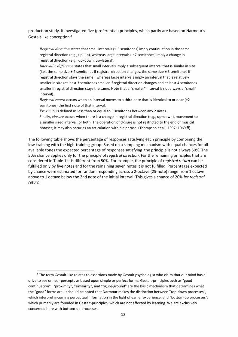
4.2 The attraction algorithm In this subsection, I will discuss how Lerdahl (1996) and Lerdahl and Krumhansl (2007) extend the model just presented to the level of the individual pitch sequence. In order to model the dynamics of attraction we need besides a general context c (normally established by a certain key), a cue tone l

(or a sequence of cue tones 𝑙𝑙) and a probe pitch k whose attraction value in the environment c+l has to be calculated. The attraction algorithm proposed by Lerdahl (1996) gives the following formula to calculate the (relative) attraction from pitch l to pitch k. Note that the context c defines the basic tonal space including the tonic triad.

(3) 𝐹𝐹𝑐𝑐(𝑘𝑘|𝑙𝑙) = 𝑠𝑠(𝑘𝑘)𝑠𝑠(𝑙𝑙)

∙ 1𝑛𝑛2

, with 𝑠𝑠(𝐶𝐶) = 4, 𝑠𝑠(𝐴𝐴,𝐺𝐺) = 3, 𝑠𝑠(𝐷𝐷,𝐹𝐹,𝐴𝐴,𝐵𝐵) = 2, 𝑠𝑠(𝑋𝑋♭) = 1

Hereby s(k) is the anchoring strength of pitch k in the basic tonal pitch space. In the previous

section, we have assumed 5 levels of description and 5 as the highest possible number of embedding (following Lerdahl, 1988). Lerdahl (1996) has eliminated the level B in his attraction model. As a consequence, he is using the expression s(k) = 4 − ce(k) for the anchoring strength. This gives identical embedding distances (and anchoring strengths) for the pitches E and G, in contrast to the original

model including level B. In formula (3), the proportion 𝑠𝑠(𝑘𝑘)𝑠𝑠(𝑙𝑙)

of the two anchoring strengths is

multiplied by a factor 1𝑛𝑛2

, where the number n counts the semitones between pitch k and pitch l. For

instance, when calculating the attraction from D to C (relative to key = C major), we get 𝐹𝐹(𝐶𝐶|𝐷𝐷) = 42∙

122

= ½. The highest value we get when considering the attraction from B to C: 𝐹𝐹(𝐶𝐶|𝐵𝐵) = 42∙ 112

= 2.

Note that the attraction function is not symmetric. For instance, the attraction from C to B is

𝐹𝐹(𝐵𝐵|𝐶𝐶) = 24∙ 112

= ½, i.e. only one quart of the attraction 𝐹𝐹(𝐶𝐶|𝐵𝐵) from B to C. Obviously, the

inverse quadratic distance dependency is borrow from physics. We find it for forces between electric charges. Another example is the classical formula for calculating the gravitation force between two mass points. What about the pendant of the anchoring strength in physics? In the first case, it relates to the charge in electrodynamics, in the second case it relates to the mass in gravitation. However, instead of the asymmetric quotient, the (symmetric) product function applies in the physical cases. This makes the physical forces symmetric, in sharp contrast with the musical forces that are always asymmetric.

It should be mentioned that many other authors have proposed similar formulas. In my opinion, the creation of such formulas and the extensive efforts of data fitting using such formulas does not really lead to a deeper musical understanding of what goes on. For an overview of several approaches, the reader is referred to Larson (2012). It is important to see that an understanding of music requires more than assuming gravity-like forces:

If music was simply a matter of following gravity-like attractions from note to note, there would be nothing for the composer to do: a melody would be as inevitable as the path of water rushing down a mountainside. The key to music is that these pulls can be resisted. It is the job of the musician to know when and how to do so. (Ball 2010: 97)

The extra resources that are ignored in the origin attraction algorithm but which are essential for real musical understanding is the role of the context and how the attraction forces interact in connection with chords and multiple voices. Lerdahl (1996) and Lerdahl and Krumhansl (2007) have modified the

20

original mechanism in order to account for such effects. However, even if the experimental fits between model and data can be improved, there remains some theoretical sadness. A real requires more than data fitting. It requires a general theoretical motivation; it requires a real grounding of the introduced formulas. This makes the difference between theory and model. A proper theory should be able to derive particular rules or laws by general principles which have an independent motivation in the field of exploration. For example, there are general cognitive respects that motivate the asymmetry of tonal forces. However, these cognitive aspects, which do not have a real pendent in the physical domain, do not play a visible and principled role in deriving formulas such as formula (3).

4.3 Intermezzo: Optimality theory and harmony theory Optimality Theory (OT) and Harmony Theory (HT) (sometimes called Harmonic Grammar) are applied in linguistics (Prince & Smolensky, 1993/2004; Smolensky & Legendre, 2006) and cognitive psychology (Gigerenzer & Selten, 2001). Both theories aim to integrate several aspects of cognition witch each other: constraint based knowledge representation systems, generative grammar, cognitive processing skills, and neural network processing. The conceptual centre of both theories is the idea of knowledge representation by violable constraints. These constraints can be grammatical principles or declarative units of common sense knowledge.

OT was initiated by Prince & Smolensky (1993/2004) as a new phonological framework that deals with the interaction of violable constraints. In recent years, OT was the subject of lively interest also outside phonology. Students of morphology, syntax and natural language interpretation became sensitive to the opportunities and challenges of the new framework (Blutner & Zeevat, 2004).9 HT is somewhat older than OT. It was introduced in the context of connectionist modelling and with the aim to overcome the gap between symbolic and subsymbolic processing (Smolensky, 1986).

An important aspect of HT is that for the modelling of cognitive behaviour (especially, perception and production) the weighted sum of the constraints counts. This relates to the assumption of cumulativity: the degree of unacceptability of a structure increases with the number of constraint violations it incurs. Related things can be said about production frequencies.10 To be sure, the term sum can be taken literal. If we see constraints as giving the value 1 if satisfied and the value 0 when not satisfied, then we can built the weighted sum of such constraint functions.

To make the point a bit more technically, let us assume a system of numerical constraint {𝐶𝐶𝑖𝑖}1≤𝑖𝑖≤𝑛𝑛. For an object x, a binary constraint Ci can have the values 0 or 1; it is violated iff Ci(x) = 0 otherwise it is satisfied. Graded constraints can have any real number as value; the higher the value, the better the constraint is satisfied. The harmony H of an object x is the sum (4) 𝐻𝐻(𝑥𝑥) = ∑ 𝑤𝑤𝑖𝑖

𝑛𝑛𝑖𝑖=1 ∙ 𝐶𝐶𝑖𝑖(𝑥𝑥), with the weight factors 𝑤𝑤𝑖𝑖

The constraint functions 𝐶𝐶𝑖𝑖(𝑥𝑥), which constitute the harmony function are also called base functions. In HT, which is based on the so-called Boltzmann machine (Hinton & Sejnowski, 1986), a

9 The reasons for linking scientists into this new research paradigm is manifold: (a) the aim to decrease the

gap between competence and performance, (b) interest in an architecture that is closer to neural networks than to the standard symbolist architecture, (c) the aim to overcome the gap between probabilistic models of language and speech and the standard symbolic models, (d) the logical problem of language acquisition, (e) the aim to integrate the synchronic with the diachronic view of language.

10 Jäger and Rosenbach (2006) have shown that cumulativity is instantiated in both frequency data and acceptability data on genitive formation in English.

21

nonlinear transformation (sigmoid function) applies to get a proper realization of probabilities as an additive measure function. However, in the simplest case, we can ignore this transformation and are simply concerned with a multiple linear regression analysis of the frequencies or probabilities (Keller, 2006).11 In this connection it is important to note that the weight factors 𝑤𝑤𝑖𝑖 in equation (4) do not depend on the considered objects x.

At this point, it should be clear that the main difference between Harmonic Grammar and Optimality Theory is the shift from numerical to non-numerical constraint satisfaction. Why Prince and Smolensky (1993/2004) proposed this shift, Paul Smolensky explains as follows:

Phonological applications of Harmonic Grammar led Alan Prince and myself to a remarkable discovery: in a broad set of cases, at least, the relative strengths of constraints of constraints need not be specified numerically. For if the numerically weighted constraints needed in these cases are ranked from strongest to weakest, it turns out that each constraint is stronger than all the weaker constraints combined. (Smolensky, 1995: 266)

In other words, the shift from Harmonic Grammar to Optimality Theory is a shift within the system of constraints toward the realization of what is called strict dominance: one higher ordered constraint can overpower all lower-ordered constraints. This is equivalent to an exponential weighting of the involved constraints. The relevance of the strictness of dominance OT appears to be mainly motivated by empirical findings in the domain of phonology. Recently, an exciting perspective from cultural language evolution (Kirby & Hurford, 2002) was given. Under certain condition, such behaviour in phonological systems can be modelled as an emergent property resulting from self-organizing processes of cultural evolution (Wedel, 2004).

From the point of view of its cognitive function, a possible advantage of strict dominance lies in the robustness of processing. Following a suggestion of David Rumelhart, the following argument was put forward:

Suppose it is important for communication that language processing computes global harmony maxima fairly reliably, so different speakers are not constantly computing idiosyncratic parses which are various local Harmony maxima. Then this puts a (meta-)constraint on the Harmony function: it must be such that local maximization algorithms give global maxima with reasonably high probability. Strict domination of grammatical constraints appears to satisfy this (meta-) constraint. (Smolensky 1995, note 38: 286).

In concord with this argument it is not implausible to assume that the theoretical explanation for differences between automatic and controlled psychological processes (Schneider & Shiffrin, 1977) can also be seen as an emergent effect of the underlying neural computations (Blutner, 2004). Whereas controlled processing relates to the capacity-limited processing when the global harmony maxima (= global energy minima) are difficult to grasp, automatic processing relates to a mode of processing where most local harmony maxima are global ones.

11 Myers (2012) argues that for corpus data the most useful type of weight-fitting model is the family of

loglinear models (taking the logarithm of the frequencies and probabilities). This is conform to the automatic setting of constraint weights from corpus data underlying the statistical idea of HT.

22

Both Optimality Theory and Harmonic Grammar are deeply rooted in the connectionism paradigm of information processing. Consequently, both theories do not assume a strict distinction between representation and processing. The development of these theories demonstrates a new and exciting research strategy: augmenting and modifying symbolist architecture by integrating insights from connectionism. Capacity limitation is a processing assumption. In the next section, we will see that this processing assumption can have powerful consequences of a structural kind. It concerns the underlying algebra of events the probability measure is based on. This is what can be seen as foundational argument for the psychological reality of quantum probabilities (Blutner & Beim Graben, 2015).

Another insight from recent developments of OT and HT concerns the so-called symbolic grounding problem (Harnad, 1990). In the context of constraint grounding in OT and HT it concerns the important methodological issue of independently motivating the used constraint system. The fact that a given system of constraints is able to provide an excellent fit to certain frequency data is not sufficient for justifying the involved constraints. In principle, there are two possibilities how constraints can be grounded: (i) by demonstrating the innateness of the constraints in a biologically plausible way (biological evolution); (ii) by arguing that the constraints can be grounded by a mechanism of cultural evolution (Jäger, 2007; Kirby & Hurford, 1997).12

4.4 The implication realization model In this part I will come back to the principles of melodic implication as developed in Narmour’s (1991, 1992) implication-realization model. A melodic implication occurs when a melodic event generates expectations for subsequent melodic events. Interestingly, Narmour’s model is applicable for both the generation and the perception of melodic structure. In generation, it builds a kind of plan for the generation of subsequent pitches. In perception, the theory is shaped by the ability to detect melodic implications and to construct relevant prediction on future events.

In Section 3.2, I have already introduced several of Narmour's preferential constraints. Narmour sees such constraints as grounded in Gestalt psychology. A consequence of this conception is that these constraints are assumed to be innate. They do not have to be learned in order to be effective. This relates to OT and HT discussed in the previous section. So far, both theories have important and interesting applications in linguistics, particularly in phonology. The step toward applying it to music theory is a great step forward to a uniform science of cognition.

12 The work of Huron (2001) can be seen in the context of grounding by cultural evolution even when the

author not explicitly refers to evolutionary mechanisms. Huron aims to derive the rules of voice leading from perceptual principles. The former can be seen as implicit rules composers normally try to follow whereas the latter can be seen as based on innate perceptual principles. Rules of voice leading "pertains to the manner in which individual parts or voices move from tone to tone in successive sonorities" (Huron 2001: 2). Huron's derivation is informal and intuitive. However, it convincingly suggests that good composer should "follow" the rules in order to be able to perceive the intended separate voices. One example is Huron's (2001: 34) "Avoid Unisons Rule. Avoid shared pitches between voices." Obviously, this rule is an immediate consequence of the perceptive principle that "effective stream segregation is violated when tonal fusion arises" (Huron 2001: 34). The underlying stability condition of cultural evolution is that producers should be able to produce musical pieces that fulfil their own intentions. Otherwise the have to modify their products. It should be noticed that there is an important difference between cultural evolution in language and music. In natural language, each speaker can also act as a listener and vice versa. This is not valid in music and other arts. Here it is only the composer who produces the music and who listens to his own music. This strongly restricts the process of cultural evolution which is not based on communication in the sense of Grice (1957).

23

As before, we assume a system of (binary or graded) numerical constraint {𝐶𝐶𝑖𝑖}1≤𝑖𝑖≤𝑛𝑛. And we assume the validity of formula (4). In the case of a linear regression model of frequencies, this sum is directly taken as being proportional to the frequency values f(x), in a loglinear model it is the logarithm of the harmony that is proportional to the frequency.

There are several examples of applying linear regression models to fit attraction values. For instance, Krumhansl (1995) compared the linear model with her own data and Larson (2012) did it with the data provided by Lake (1987). Cuddy and colleagues (Cuddy & Lunney, 1995; Thompson et al., 1997) also have tested the model empirically by investigating melodic expectancies in a melody-completion task. Let me concentrate the debate on the analysis performed by Krumhansl (1995). Using the constraints discussed in Section 3.2, Krumhansl treated the constraints registral direction, intervallic difference, and registral return as all-or-none (value 1 if satisfied, value 0 if not). In contrast, the principles proximity and closure were treated as graded in strength (proximity on 7 levels from 0, …, 6; closure on three levels 0, 1, 2). Further, two additional constraints were considered: Tonality which mimics the static attraction values discussed in Section 4.1 and a constraint called Unison. The material used in Krumhansl's (1995) three experiments consist of British folksongs, Webern's "atonal" songs, and Chines folksongs.

The weighted sum of the constraints was fitted to the three sets of experimental frequency data. The correlation function between fitted model and data was high: r = 0.84 for the British folksongs; r = 0.71 for Webern's "atonal" songs; r = 0.85 for the Chines folksongs. However, this is result is not automatically an evidence for the adequateness of the involved constraints. Some constraints were very week – the weakest contribution was made by intervallic difference. The strongest contribution were made by proximity and registral return. Larson (2004) suggests that the results of the fit do not show much more than these two simple statistical regularities: “added notes are usually close in pitch to one of the two preceding notes” (proximity) and “large leaps are usually followed by a change in direction” (registral return). In a careful analysis, Schellenberg (1996, 1997) concludes that the bottom-up component of Narmour’s model can be simplified to something like these two constraints without a substantial loss of the amount of correlation with the experimental results.

At this point let us conclude that it is a huge methodological problem to demonstrate that the assumed constraints are psychologically adequate. It is not enough to demonstrate that the cumulatively provide a good fit for the data. It also is required to demonstrate their independence and the absence of redundancy. In Larson's (2012) book is demonstrated that most constraints are not really important (do not contribute) and others even have a negative effect. The real methodological issue is this: How can we ground the selected constraints? This is one aspect of the symbolic grounding problem (Harnad, 1990) – an unsolved problem in the domain of cognitive music theory, so far I can see.

4.5 The metaphoric theory of musical forces Several authors explicitly or implicitly use the ideas of musical movements and musical forces as based on conceptual metaphors in the sense of Lakoff and Johnson (1980). That means the source domain of naïve (folk) physics is assumed to constitute a conceptual network establishing main propositions about physical movements and their causes ‒ the physical forces. Analogical reasoning is used then to transfer the physical concepts to the goal domain of tonal music. In this way, it is

24

possible to describe the most plausible expectations a listener generates during the processing of tonal music. This includes expectations based on static and dynamic forces.13

In this subsection, I will present the basic ideas of Steve Larson as published in his last book (Larson 2012). I think that this book gives the best overview on the field of musical forces presently available. And it provides a fair discussion on related proposals such as Narmour's (1992) implication-realization model, the model of Bharucha (1996), Lerdahls (2001) algorithm, and related ideas of Margulis (2003) and others.

Three of these forces I call "gravity" (the tendency of an unstable note to descend), "magnetism" (the tendency of an unstable note to move to the nearest stable pitch, a tendency that grows stronger the closer we get to a goal), and "inertia" (the tendency of a pattern of musical motion to continue in the same fashion, where what is meant by "same" depends upon what that musical pattern is "heard as"). (Larson, 1997, p. 102)

To give an example, assume the context is c-minor and a melodic beginning G-F is given. "Musical gravity" is satisfied by going down: G-F-E. For "magnetism", an assumption about the "stable pitches"

is required. Let us assume that these pitches are formed by the harmonic triad, i.e. {C, E♭, G}. The

considered sequence G-F-E♭ could be assumed to satisfy "magnetism". In Larson (2002) and Larson and van Handel (2005) however this is doubt. "Magnetism" is assumed to be satisfied only if the

probe tone is element of the tonic triad and it resolves by half step.14 Hence, C-D-E♭ satisfies the

constraint "magnetism" but G-F-E♭ does not. Obviously, both the sequence G-F-E♭ and C-D-E♭ satisfies "inertia".

Table 3 shows the relevant constraints and their scores for a selection of melodic beginnings and

probe tones as adapted from Larson and van Handel (2005). The established key are c- and f♯-minor

in the first eight pattern and C- and F♯-major in the last eight pattern. In all cases the harmonic triad can be written as {1̂, 3̂, 5̂} using the key-dependent notation for elements of a diatonic scale introduced in Section 3.2.5.

The empirical hypothesis is tested that the average rating of each of the investigated patterns is a function of the sum of musical forces acting on that pattern. Hence, a linear regression analysis is performed testing the following hypothesis for the "net force" F for a probe tone x as reflected by the ratings:

(5) F(x) = wG ⋅ G(x) + wM ⋅ M(x) + wI ⋅ I(x)

13 Larson (2012) gives some examples that concern ordinary discourses about music. They demonstrate

the metaphorical potential of the force conception: GRAVITY: The soprano's high notes rang above. The rising melodic line climbed higher. MAGNETISM: The music is drawn to this stable note. The leading tone is pulled to the tonic. INERTIA: The accompanimental figure, once set in motion… . This dance rhythm generates such momentum that… .

14 That means the distance between the second tone of the melodic beginning and the probe tone is exactly a half tone, and the probe tone is an element of the tonic triad. Larson (2002) found that for the chosen selection of melodic beginnings and probe tones this constraint of "magnetism" works best. Larson (2012) also considers modifications of this constraint.

25

Hereby, wG , wM , and wI are the corresponding weight factors of the three constraint functions. The results of the linear regression analysis for Larson's and van Handel's data are wG = 0.4, wM = 0.1, wI = 1.2. The correlation between model and data is r = 0.95. This high r-value means that the three forces, taken together, can account for about 90% of the variance of the frequency data. The two weight factors for gravity and magnetism are each significantly different from zero (at a 0.1 % level), but the weight for inertia is not. Interestingly, other studies using other data sets (Larson 2002) give a different result: gravity and inertia both make significant contributions but magnetism does not. In the 2005 study an additional analysis was performed that included in addition to GRAVITY, MAGNETISM, and INERTIA, an extra factor signaling the ending on tonic (= 1̂) was introduced. In this case the correl-ation is still a bit higher: r = 0.977, and the extra factor got a weight of 0.46. Interestingly, the other factors now get weights different from the former analysis: wG = 0.16 (instead of 0.4), wM = 0.26 (instead of 0.1), and wI = 1.2 (as before). Hence, magnetism and inertia both make significant contrib-utions to linear regression but gravity does not. This demonstrated that the contribution of single factors to the "net force" can be evaluated only when the full context of all involved factors is given.

Finally, I want to stress that even a high correlation value of the fit as found in the data analysis just described does not answer the fundamental question about constraint grounding. As we have seen, the addition of some extra factors can radically change the influence of other factors and can even marginalize some factors. Hence, a multiple regression analysis with a high overall correlation coefficient cannot be taken as argument that the involved factors are all substantiated and "symbolically grounded" in the sense of Harnad (1990).

I think Larson (2012) was aware of this problem. Several of his careful analyses try to justify the special role of musical forces. This contrast with alternative analyses by earlier authors. Further, Larson (2012) has investigated different variants of various factors (constraints) and he found how sensitive the cognitive system reacts even on minimal variations. However, he did not perform analyses that systematically varied the content of the involved factors and constraints as it was realized recently in the field of linguistic semantics and pragmatics in connection with the symbolic grounding problem (Jäger, 2004, 2007; Kirby & Hurford, 1997; Mattausch, 2004; Wedel, 2004). The proposed mechanisms such as bidirectional learning are mechanisms of cultural learning.15 However, grounding is also possible in purely biological terms, for instance when it is assumed that musical forces ("tensions") can be thought as arising from deviations of the Gestalt principles (as noted by Larson (2012) in Section 9). The hypothesis of a biological grounding could be substantiated by assuming connectionist models, which are very appropriate for confirming nativist elements of cognitive grounding (Elman, 1998; Smolensky & Legendre, 2006)

4.6 Interval cycles In recent research, Matthew Woolhouse has proposed to explain tonal attraction in terms of interval cycles (Woolhouse, 2009, 2010; Woolhouse & Cross, 2010). The basic idea is that the attraction between two pitches is proportional to the number of times the interval spanned by the two pitches must be multiplied by itself to produce some whole number of octaves. Assuming twelve-tone equal temperament, the interval-cycle proximity (ICP) of the interval can be defined as the smallest positive number icp such that the product with the interval length (i.e. the number of half tone steps spanned

15 In linguistics, each agent involved in the process of cultural evolution can take both the role of the

Speaker and the role of the Listener. This is different in music and other arts where not everybody usually acts as producer. Hence, bidirectional learning is restricted to a small subgroup only (called composers). The other members of the community act as receivers only and process the given of musical inputs.

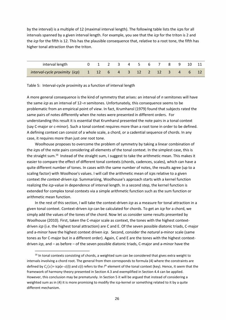
26

by the interval) is a multiple of 12 (maximal interval length). The following table lists the icps for all intervals spanned by a given interval length. For example, you see that the icp for the triton is 2 and the icp for the fifth is 12. This has the plausible consequence that, relative to a root tone, the fifth has higher tonal attraction than the triton.

interval length 0 1 2 3 4 5 6 7 8 9 10 11

interval-cycle proximity (icp) 1 12 6 4 3 12 2 12 3 4 6 12

Table 5: Interval-cycle proximity as a function of interval length A more general consequence is the kind of symmetry that arises: an interval of n semitones will have the same icp as an interval of 12–n semitones. Unfortunately, this consequence seems to be problematic from an empirical point of view. In fact, Krumhansl (1979) found that subjects rated the same pairs of notes differently when the notes were presented in different orders. For understanding this result it is essential that Krumhansl presented the note pairs in a tonal context (say C-major or c-minor). Such a tonal context requires more than a root tone in order to be defined. A defining context can consist of a whole scale, a chord, or a cadential sequence of chords. In any case, it requires more than just one root tone.

Woolhouse proposes to overcome the problem of symmetry by taking a linear combination of the icps of the note pairs considering all elements of the tonal context. In the simplest case, this is the straight sum.16 Instead of the straight sum, I suggest to take the arithmetic mean. This makes it easier to compare the effect of different tonal contexts (chords, cadences, scales), which can have a quite different number of tones. In cases with the same number of notes, the results agree (up to a scaling factor) with Woolhose's values. I will call the arithmetic mean of icps relative to a given context the context-driven icp. Summarizing, Woolhouse's approach starts with a kernel function realizing the icp-value in dependence of interval length. In a second step, the kernel function is extended for complex tonal contexts via a simple arithmetic function such as the sum function or arithmetic mean function.

In the rest of this section, I will take the context-driven icp as a measure for tonal attraction in a given tonal context. Context-driven icp can be calculated for chords. To get an icp for a chord, we simply add the values of the tones of the chord. Now let us consider some results presented by Woolhouse (2010). First, taken the C-major scale as context, the tones with the highest context-driven icp (i.e. the highest tonal attraction) are C and E. Of the seven possible diatonic triads, C-major and a-minor have the highest context driven icp. Second, consider the natural a-minor scale (same tones as for C-major but in a different order). Again, C and E are the tones with the highest context-driven icp, and – as before – of the seven possible diatonic triads, C-major and a-minor have the

16 In tonal contexts consisting of chords, a weighted sum can be considered that gives extra weight to

intervals involving a chord root. The general from then corresponds to formula (4) where the constraints are defined by 𝐶𝐶𝑖𝑖(𝑥𝑥)= icp(x−c(i)) and c(i) refers to the ith element of the tonal context (key). Hence, it seem that the framework of harmony theory presented in Section 4.3 and exemplified in Section 4.4 can be applied. However, this conclusion may be prematurely. In Section 5 it will be argued that instead of considering a weighted sum as in (4) it is more promising to modify the icp-kernel or something related to it by a quite different mechanism.

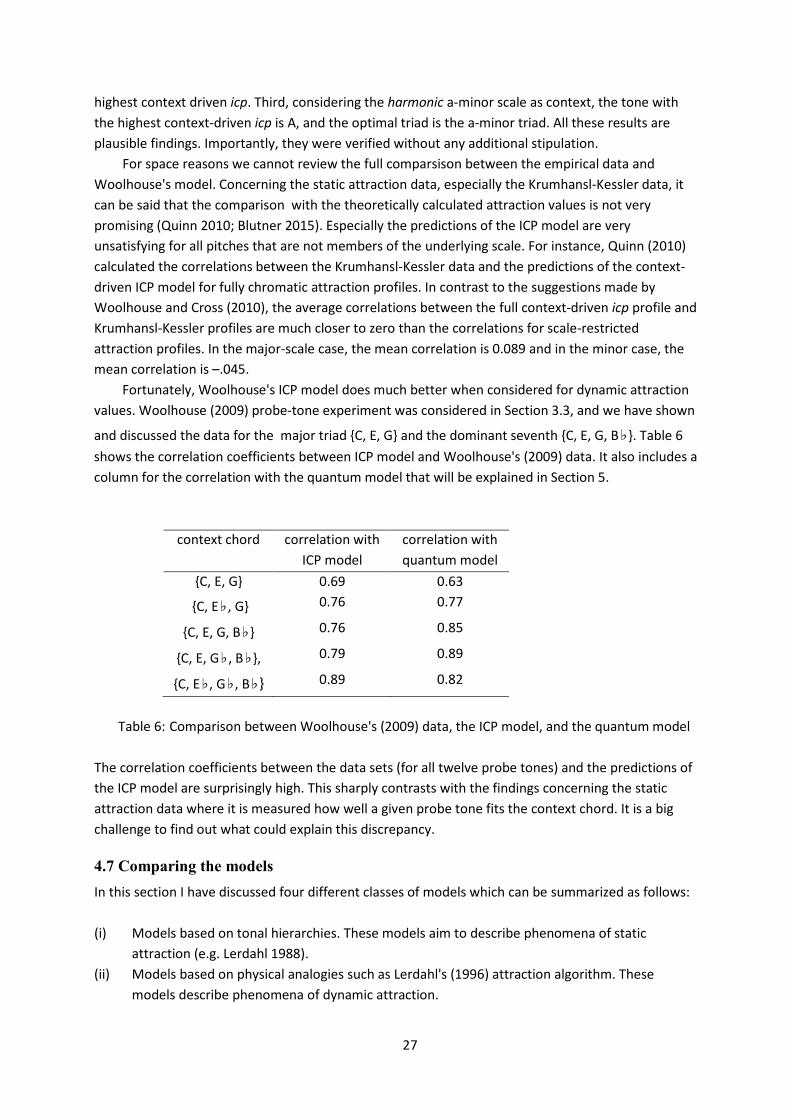
27

highest context driven icp. Third, considering the harmonic a-minor scale as context, the tone with the highest context-driven icp is A, and the optimal triad is the a-minor triad. All these results are plausible findings. Importantly, they were verified without any additional stipulation.

For space reasons we cannot review the full comparsison between the empirical data and Woolhouse's model. Concerning the static attraction data, especially the Krumhansl-Kessler data, it can be said that the comparison with the theoretically calculated attraction values is not very promising (Quinn 2010; Blutner 2015). Especially the predictions of the ICP model are very unsatisfying for all pitches that are not members of the underlying scale. For instance, Quinn (2010) calculated the correlations between the Krumhansl-Kessler data and the predictions of the context-driven ICP model for fully chromatic attraction profiles. In contrast to the suggestions made by Woolhouse and Cross (2010), the average correlations between the full context-driven icp profile and Krumhansl-Kessler profiles are much closer to zero than the correlations for scale-restricted attraction profiles. In the major-scale case, the mean correlation is 0.089 and in the minor case, the mean correlation is –.045.

Fortunately, Woolhouse's ICP model does much better when considered for dynamic attraction values. Woolhouse (2009) probe-tone experiment was considered in Section 3.3, and we have shown

and discussed the data for the major triad {C, E, G} and the dominant seventh {C, E, G, B♭}. Table 6 shows the correlation coefficients between ICP model and Woolhouse's (2009) data. It also includes a column for the correlation with the quantum model that will be explained in Section 5.

context chord correlation with ICP model

correlation with quantum model

{C, E, G} 0.69 0.63

{C, E♭, G} 0.76 0.77

{C, E, G, B♭} 0.76 0.85

{C, E, G♭, B♭}, 0.79 0.89

{C, E♭, G♭, B♭} 0.89 0.82

Table 6: Comparison between Woolhouse's (2009) data, the ICP model, and the quantum model

The correlation coefficients between the data sets (for all twelve probe tones) and the predictions of the ICP model are surprisingly high. This sharply contrasts with the findings concerning the static attraction data where it is measured how well a given probe tone fits the context chord. It is a big challenge to find out what could explain this discrepancy.

4.7 Comparing the models In this section I have discussed four different classes of models which can be summarized as follows: (i) Models based on tonal hierarchies. These models aim to describe phenomena of static

attraction (e.g. Lerdahl 1988). (ii) Models based on physical analogies such as Lerdahl's (1996) attraction algorithm. These

models describe phenomena of dynamic attraction.

28

(iii) Woolhouse's attraction model in terms of interval cycles (Woolhouse, 2009, 2010; Woolhouse & Cross, 2010). This model was applied for both attraction types.

(iv) Models based on linear and log-linear regression. The most important representatives of this account are Narmour’s (1991, 1992) implication-realization model of melodic expectations and Larson's (2012) metaphoric theory of musical forces.

Empirically, the hierarchical model gives an adequate description for the static attraction profiles. This concerns a first important finding, namely that for both major and minor profiles, scalar tones have higher values of tonal attraction than non-scalar tones. With reference to a piano this means that the white tones have higher values than the black tones (when considering C-major or a-minor). A second general finding is that all tones of the tonic triad have higher values than other tones of the scale (Temperley 2007: 84). These two important empirical facts are directly stipulated by the hierarchic model: by assuming a "diatonic space" (level D) which includes all scalar notes and by assuming a higher order "triadic space" (level C) that includes the tones of the triadic space.17 The stipulations of the hierarchic model concern the number of levels and the precise content of some levels. For instance, they concern the question of which chords constitute the triadic level. For Western music, the decision is easy to make by assuming that we have a clear distinction between major and minor systems. Non-Western kinds of music need not conform to the major/minor system and can be based on tonal scales quite different from those of Western music. Alternative scales such as Indian ragas or the scales underlying traditional Japanese music are widely used in world music. It is not completely clear how we can modify or extend the hierarchical model in order to account for the traits of these kinds of music.

The second group of models including Lerdahl's attraction algorithm can be criticized for a similar reason: The models give a description but no explanation. This leads us to the third group of models that includes the ICP model. This model is important from a methodological point of view. The model seeks to derive the basic traits of major and minor attraction profiles, rather than to stipulate them. In the ICP model, absolute profiles are defined, taking interval-cycle proximity as an absolute function of interval length. These absolute profiles are key-independent. Absolute profiles are theoretical entities, i.e. they cannot directly be observed empirically. They abstract from the underlying tonal context, which in Western music is defined by a major or a minor scale.18 A capital advantage of this approach is that it can also be applied to non-Western kinds of music. From the empirical point of view, the model is not really convincing, especially if we consider the full context-driven ICP-profiles for the static attraction data and the Huron (2007) data for chords (cf. Blutner 2015).

The last group of models is based on a linear or log-linear regression analysis. A big challenge for this kind of models is the right choice and independent motivation of the underlying system of

17 Another finding is that for major scales the tonic pitch has a higher attraction value than the fifth. In the

hierarchic model, this suggests the assumption of an open fifth space (level B). Unfortunately, this conflicts with the Kostka-Payne corpus data (Kostka & Payne, 1995). Consequently, the existence of this level of fifth space is questionable, for it does not apply for all assumed tonal scales.

18 Assume we perform an empirical study asking for the proximity between two pitches without explicitly presenting a context. It would be wrong to assume that we can measure the absolute profiles in this way. Instead, the subjects will automatically infer a tonal scale, i.e. they will decide about a scale which fits best into the presented pitch interval (and normally, the two pitches are assumed both to be elements of the inferred scale). Hence, we will get a profile relative to an inferred scale.

29

constraints. Larson's systems inspirited by the metaphoric theory of tonal forces possibly is the best choice. However, there is the open issue of providing an independent motivation of the constraints either by arguments from cultural or biological evolution.

Summing up, the hierarchical model has some serious conceptual and empirical flaws. In contrast, the ICP-model makes an interesting methodological point. It tries to derive the observed phenomena and to fit the empirical data by assuming only one important principle: the principle of interval-cycle proximity. The model is successful for the dynamic attraction values. Unfortunately, it is descriptively inadequate for the static attraction values. The last group of models that were considered in this section are models based on linear and log-linear regression. I have pointed out that these models conform to the framework of harmony theory widely used in cognitive and computational linguistics.

In the following section, I will introduce a simple quantum model of tonal attraction (based on a single qubit). This model resolves the issue of integrating static and dynamic attraction values. Moreover, it gives an answer to the grounding problem of constraints handled by the existence of symmetries in tonal music. This research line extends the constraint-based treatment of tonal forces. Section 6 will extend the simple model and introduce aspects of quantum field theory, and especially consider to role of gauge forces. They relate to musical micro-forces, which are at a different level of description than the phenomenological forces discussed in folk theories of music.

5. The qubit model of tonal attraction In this section, I will develop a quantum model of tonal music that is founded on a single qubit. In order to avoid any potential confusion, let me note that the term "quantum" does not relate to any physical reductionism that aims to reduce cognitive phenomena to physical ones as proposed for the psychology of consciousness by Hameroff and Penrose (1995). These authors propose an "orchestrated reduction of quantum coherence in brain microtubules". The present approach is leaded by a new approach to cognitive science called "quantum cognition".19 The basic insight of this approach is that the mathematical instruments developed in quantum physics are not only applicable to physical phenomena of tiny particles but also to the macro-world of cognitive psychology.

Here is a sketch of the proposal as developed in the next subsections. First, following my earlier article (Blutner, 2015), I propose to represent the twelve tones as vectors ψk in a two-dimensional Hilbert space. Using the idea of a Bloch-circle (see appendix A1) it is shown that the twelve tones can be arranged according to the circle of fifth used in standard (Riemannian) music theory. Second, given a single pitch 𝑙𝑙 as context and a probe tone 𝑘𝑘, the value of a kernel function 𝐾𝐾(𝑘𝑘 − 𝑙𝑙) can be calculated. The kernel is defined by the square of the length of the projection of the vector ψk on the vector ψl. In the simplest case of zero phases, the kernel is 𝐾𝐾(𝑘𝑘 − 𝑙𝑙) = cos2 (𝜋𝜋(𝑘𝑘 − 𝑙𝑙) 12⁄ . We will call this kernel the neutral kernel. Borrowing the idea from markedness theory in linguistics (Chomsky & Halle, 1968; Kean, 1995; Smolensky & Legendre, 2006), it describes the unmarked case (default case or neutral case are alternative names for the same idea). Typically, the neutral kernel is assumed to correspond with innate knowledge structures. The values of the kernel functions can be seen as defining the static attraction value of a probe tone 𝑘𝑘 given a single cue tone 𝑙𝑙 (see Blutner, 2015). Third, assuming the context consist of a chord, a cadence, or a tonal series, then the static

19 For an concise introduction into the field the reader is referred to the excellent book by Busemeyer and

Bruza (2012). In the appendix to this article we present the basic mathematical ideas of this approach that are needed for understanding the application to tonal music.

30

attraction value is the average of the attraction values relative to the contexts of the involved single tones. Fourth, in Blutner (2015) I have argued that a considerable improvement of the model can be achieved when the phase parameters are considered and fitted to the available static attraction data. The inclusion of the phase parameters defines a modified kernel function (also called marked kernel). The fifth point concerned a novel idea. We can approach the dynamic attraction data by performing a uniform phase shift of the tones in the context chord(s) (letting the probe tones unaffected). Hence, only one new parameter is needed for describing the phase shift and for determining the dynamic attraction values. In the following subsections, I will explain the story in detail – highlighting the role of symmetries for fixing the neutral kernel and the role of gauge fields for modifying it.

5.1 Symmetry groups and the principle of translation invariance One of the fundamental ideas of quantum cognition is to apply the mathematics of the physical formalism to the domain of cognition. For example, we can use a series of qubit states to represent the twelve pitch classes used in tonal music. In addition, we can use the probability that one of these qubit state collapses into another one as a measure for the tonal attraction between the corresponding tones.

In Section 3, we have introduced a numeric notation to define the twelve tones of the system. For convenience, it is repeated here:

(1) 0 = C, 1 = C♯, 2 = D, 3 = D♯, 4 = E, 5 = F, 6 = F♯, 7 = G, 8 = G♯, 9 = A, 10 = B♭, 11 = B There are certain actions or operations that allow transforming tones into other tones. For instance, we can increase the tones by a certain number of steps (0, 1, 2, …, 11). Such actions are called

translations. The 1-step translation transforms C into C♯, C♯ into D, and so on. Actions can be combined. For example, we can combine the translation of a 2-step increase with a 3-step translation, resulting in a 5-step translation (in other words, a major second combined with a minor third gives a fifth). We will denote these operations likewise with the numbers 0, 1, 2, …, 11. Normally, the context makes clear what the numbers denote: a pitch class or the operation of increasing tones by a number of elementary steps. It is obvious that the combination of acts of translations can be described by addition (modulo 12): x + y mod 12; e.g., 2+3 mod 12 = 5, 7+6 mod 12 = 1. For a concise introduction of basic concepts of the mathematical theory of groups, the reader is referred to the appendix.

In the case of music based on twelve tones, we have to consider the set of group elements {0, 1, 2, …, 11}, and the group operation is x ⋅ y = x + y mod 12. The neutral element is the element denoted by 0: (0 + x) mod 12 = (x + 0) mod 12 = x. For the inverse element x−1, we have x−1 = (12 − x) mod 12.

The group consisting of the 12 tones is a cyclic group, which is called ℤ12 (see appendix A2). In the

present numerical representation of the cyclic group ℤ12 we have four generators conforming to the numbers 1, 11, 7, 5. Hence, 1 (upward) and 11 (downward) generate the sequence of semitones. In addition, the elements 5 and 7 enumerate the group elements in successive fifths or fourths − representing the circle of fifths. If x is an integer variable running from 0 to 11, we can generate the group elements in the respective four cases in the following way, where the variable x runs from 0 to 11:

(6) a) x+1 mod 12

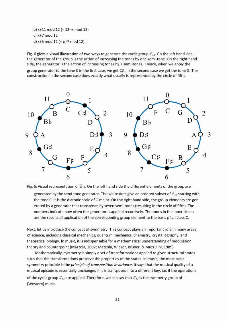
31

b) x+11 mod 12 (= 12−x mod 12) c) x+7 mod 12 d) x+5 mod 12 (= x−7 mod 12).

Fig. 6 gives a visual illustration of two ways to generate the cyclic group ℤ12. On the left hand side, the generator of the group is the action of increasing the tones by one semi-tone. On the right hand side, the generator is the action of increasing tones by 7 semi-tones. Hence, when we apply the group generator to the tone C in the first case, we get C♯. In the second case we get the tone G. The construction in the second case does exactly what usually is represented by the circle of fifth.

Fig. 6: Visual representation of ℤ12. On the left hand side the different elements of the group are

generated by the semi-tone generator. The white dots give an ordered subset of ℤ12 starting with the tone 0. It is the diatonic scale of C-major. On the right hand side, the group elements are gen-erated by a generator that transposes by seven semi-tones (resulting in the circle of fifth). The numbers indicate how often the generator is applied recursively. The tones in the inner circles are the results of application of the corresponding group element to the basic pitch class C.

Next, let us introduce the concept of symmetry. This concept plays an important role in many areas of science, including classical mechanics, quantum mechanics, chemistry, crystallography, and theoretical biology. In music, it is indispensable for a mathematical understanding of modulation theory and counterpoint (Mazzola, 2002; Mazzola, Wieser, Bruner, & Muzzulini, 1989).

Mathematically, symmetry is simply a set of transformations applied to given structural states such that the transformations preserve the properties of the states. In music, the most basic symmetry principle is the principle of transposition invariance. It says that the musical quality of a musical episode is essentially unchanged if it is transposed into a different key, i.e. if the operations

of the cyclic group ℤ12 are applied. Therefore, we can say that ℤ12 is the symmetry group of (Western) music.

0 1

2

3

4

5 6

7

8

9

10

11

C C♯

D

D♯

E

F F♯ G

G♯

A

B♭

B

0 1

2

3

4

5 6

7

8

9

10

11

C G

D

A

E

B

F

B♭

F♯ C♯

G♯

D♯

32

In mathematics, the word representation means a structure-preserving function. In group theory, a representation is simply a homomorphism. The object of our investigation is the symmetry group of translations. The homomorphism we seek for should map this group to a more concrete group that is in some sense easier to understand than the original one. For example, this group could consist of linear maps as studied in linear algebra. More concretely, the group could consist of certain rotations of vectors in a two-dimensional vector space. For instance we can rotate the vector

ψ→ = (10) in n steps to the original vector. In linear algebra, the elementary rotation steps can be

described by the following rotation matrix 𝛾𝛾:

(7) 𝛾𝛾 = ( cos (2𝜋𝜋 𝑛𝑛⁄ ) sin (2𝜋𝜋 𝑛𝑛⁄ )− sin (2𝜋𝜋 𝑛𝑛⁄ ) cos (2𝜋𝜋 𝑛𝑛⁄ ))

One application of this matrix to the vector ϕ↑ = (01) results in the vector 𝛾𝛾 (0

1) = ( sin (2𝜋𝜋 𝑛𝑛⁄cos (2𝜋𝜋 𝑛𝑛⁄ )). This

is a rotation of the original vector by an angle of 2𝜋𝜋 𝑛𝑛⁄ . It is not difficult to see that the generator 𝛾𝛾 as

defined in (7) generates the cyclic group ℤn. For n = 12, the group elements of this group can be enumerated as follows, where k runs from 0 to 11:

(8) 𝛾𝛾𝑘𝑘 = ( cos (2𝜋𝜋𝑘𝑘 12⁄ ) sin (2𝜋𝜋𝑘𝑘 12⁄ )− sin (2𝜋𝜋𝑘𝑘 12⁄ ) cos (2𝜋𝜋𝑘𝑘 12⁄ ))

In this way, we can generate a series of vector states ψk representing the twelve tones. In (9a) these states are given as vectors in a two dimensional real Hilbert space (we have assumed zero phases). In the Bloch sphere, these vectors are represented as in (9b). The y-component is zero because of the zero phase. Hence, we are really concerned with a circle in the x-z-plane. Note that the angles in (9a) are half of the ones in (2) of appendix A2 introducing the qubit Hilbert space. Hence, the tritone in the vector picture is orthogonal to the tonic tone (angle 𝜋𝜋/2). But in the Bloch sphere the two points are on opposite sides of the sphere; hence, their angle is π.

(9) a. ψk = 𝛾𝛾𝑘𝑘 (01) = ( sin (𝜋𝜋𝑘𝑘 12⁄

cos (𝜋𝜋𝑘𝑘 12⁄ ))

b. xk = sin(𝜋𝜋𝑘𝑘 6⁄ ), zk = cos (𝜋𝜋𝑘𝑘 6⁄ ). Importantly, we have to consider two different ways of enumeration, corresponding to two

generators of the group ℤ12. One enumerates the pitches in a chromatic (ascending) way; the other enumerates the tones according to the (ascending) circle of fifth. In this way, we get two Bloch circles, which exactly correspond to the two circles shown by Fig. 6. Which of these two representations of tones is the preferred one depends of an empirical decision. This decision is not difficult in the present case because we intend to express the similarity relation between tones, tonal regions, or chords. In the next section, I will demonstrate that this clearly favours the circle of fifth.

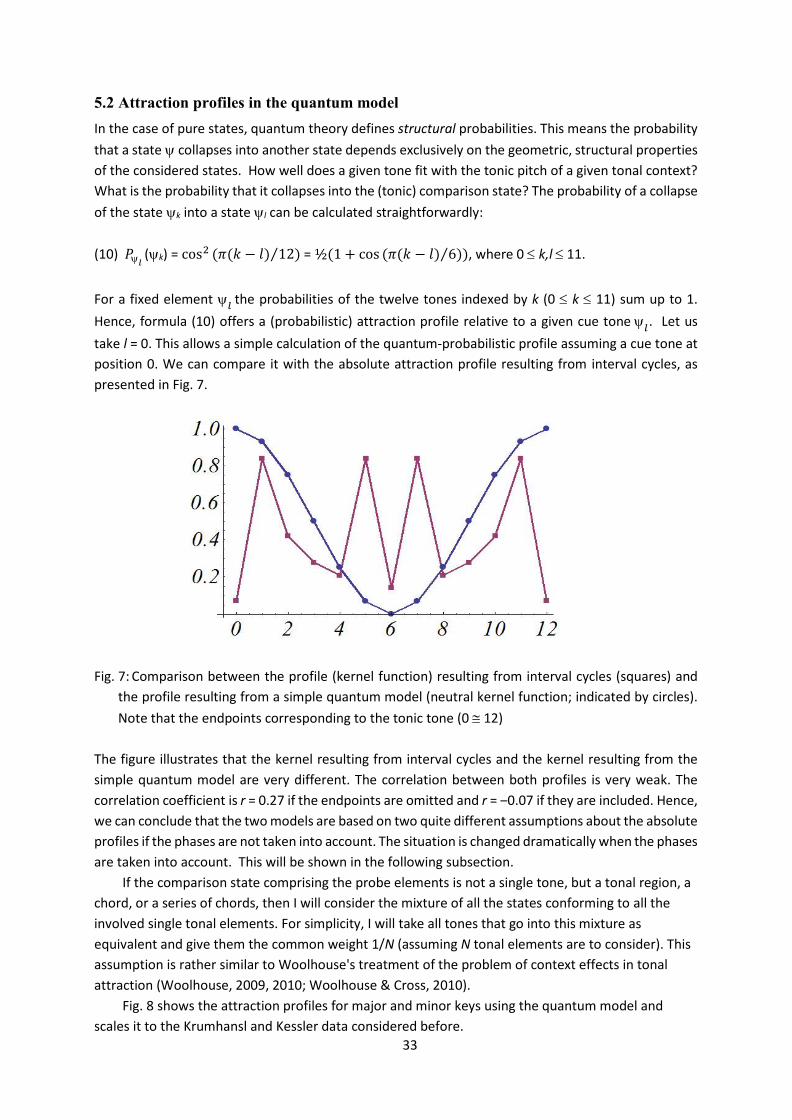
33

5.2 Attraction profiles in the quantum model In the case of pure states, quantum theory defines structural probabilities. This means the probability that a state ψ collapses into another state depends exclusively on the geometric, structural properties of the considered states. How well does a given tone fit with the tonic pitch of a given tonal context? What is the probability that it collapses into the (tonic) comparison state? The probability of a collapse of the state ψk into a state ψl can be calculated straightforwardly: (10) 𝑃𝑃ψ𝑙𝑙 (ψk) = cos2 (𝜋𝜋(𝑘𝑘 − 𝑙𝑙) 12⁄ ) = ½(1 + cos (𝜋𝜋(𝑘𝑘 − 𝑙𝑙) 6⁄ )), where 0 ≤ k,l ≤ 11.

For a fixed element ψ𝑙𝑙 the probabilities of the twelve tones indexed by k (0 ≤ k ≤ 11) sum up to 1. Hence, formula (10) offers a (probabilistic) attraction profile relative to a given cue tone ψ𝑙𝑙. Let us take l = 0. This allows a simple calculation of the quantum-probabilistic profile assuming a cue tone at position 0. We can compare it with the absolute attraction profile resulting from interval cycles, as presented in Fig. 7.

Fig. 7: Comparison between the profile (kernel function) resulting from interval cycles (squares) and

the profile resulting from a simple quantum model (neutral kernel function; indicated by circles). Note that the endpoints corresponding to the tonic tone (0 ≅ 12)

The figure illustrates that the kernel resulting from interval cycles and the kernel resulting from the simple quantum model are very different. The correlation between both profiles is very weak. The correlation coefficient is r = 0.27 if the endpoints are omitted and r = ‒0.07 if they are included. Hence, we can conclude that the two models are based on two quite different assumptions about the absolute profiles if the phases are not taken into account. The situation is changed dramatically when the phases are taken into account. This will be shown in the following subsection.

If the comparison state comprising the probe elements is not a single tone, but a tonal region, a chord, or a series of chords, then I will consider the mixture of all the states conforming to all the involved single tonal elements. For simplicity, I will take all tones that go into this mixture as equivalent and give them the common weight 1/N (assuming N tonal elements are to consider). This assumption is rather similar to Woolhouse's treatment of the problem of context effects in tonal attraction (Woolhouse, 2009, 2010; Woolhouse & Cross, 2010).

Fig. 8 shows the attraction profiles for major and minor keys using the quantum model and scales it to the Krumhansl and Kessler data considered before.

34

Fig. 8: The dashed curves show the Krumhansl-Kessler profiles (left: major keys; right: minor keys). The

bold curves are the theoretical predictions of the quantum model.

The correlation coefficient between the predicted profile and the Krumhansl-Kessler profile is r = 0.78 in the case of major keys and r = 0.69 in the case of minor keys. Remember the correlation coefficients for the full chromatics scales using the ICP model: r = 0.089 in the major case, and r = 0.045 in the minor case.20

5.3 Phase parameters and attraction profiles A qubit can be characterized by two parameters θ and ∆ as described by formula (23) of appendix A1. The parameter ∆ describes the phase shift between the two orthogonal "wave functions" ϕ↑ and ϕ→

(representing the tonic and the corresponding triton). The phase parameter ∆ was set to be zero so far. Now we will generalize the earlier model by assuming that non-zero phase shifts can be involved. That means we replace formula (9a) by the following expression for the states ψk expressing the tones including a phase shift (in an enumeration conforming to the circle of fifth)21:

(11) ψk = (sin (𝜋𝜋𝑘𝑘 12)⁄

𝑒𝑒𝑖𝑖∆𝑘𝑘 cos (𝜋𝜋𝑘𝑘 12⁄ ))

We will consider the phase parameters ∆𝑘𝑘 as free parameters that are determined by processes of self-organization and learning. Obviously, these parameters can break the symmetry that originally

conformed to the symmetry group ℤ12. In order to retain the symmetry, we will use a special method of recalibration.

The probability of a collapse of the state ψk into a state ψl can be calculated as follows (after trigonometric reductions). Hereby, we will take the index 𝑙𝑙 to represent a cue tone (context) and the index 𝑘𝑘 to represent the probe tone. Hence, the parameter ∆𝑘𝑘 refers to the phase of the probe tone and the parameter ∆′𝑙𝑙 to the phase of the cue tone. Even when the cue tone and the probe tone coincide, the parameters can still be different.

20 Since we do not know the detailed statistics of the Krumhansl-Kessler data, it cannot be decided at what

level the differences to the quantum model are significant. 21 Of course, the description of tonal states as given in (9a) or (11) should not be confused with a

description of the acoustic oscillation or waves connected with a certain pitch class. Even when the cognitive status of the state description is not completely clear, I refer to potential representations of tones as developed in Neo-Hebbian neurodynamics (Acacio de Barros & Suppes, 2009; Large, 2010).

35

(12) 𝑃𝑃ψ𝑙𝑙 (ψk) = 12

+ 14

(1 + cos(∆𝑘𝑘 − ∆′𝑙𝑙)) cos (𝜋𝜋(𝑘𝑘 − 𝑙𝑙) 6⁄ ) + 14

(1 − cos(∆𝑘𝑘 − ∆′𝑙𝑙)) cos (𝜋𝜋(𝑘𝑘 + 𝑙𝑙) 6⁄ ),

where 0 ≤ k,l < 12. In case of ∆𝑘𝑘 − ∆′𝑙𝑙 = 0 the formula (12) turns into the special case presented by formula (10). In this special case, the transfer probability depends on the difference of the frequencies 𝜋𝜋(𝑘𝑘 − 𝑙𝑙)/6 only. In the general case, however, it depends both of the sums and the differences. Concerning the phases, the difference ∆𝑘𝑘 − ∆′𝑙𝑙 is relevant in both cases. As mentioned already, transposition invariance is not valid in the general case.

There is a simple "trick" to guarantee transposition invariance in the general case: Instead of taking the absolute values k for representing the probe tones, we consider its relative distance from the contextual index 𝑙𝑙 and start counting with the number 3 (instead of 0). In technical terms, we simply recalibrate the indices by transforming 𝑘𝑘 → 𝑘𝑘 − 𝑙𝑙 + 3 and 𝑙𝑙 → 3. That mean, instead of the index k, we have the (transposition-invariant) difference 𝑘𝑘 − 𝑙𝑙 + 3 and all contextual elements are reset to pitch number 3.22 Formula (13) shows the result of the performed recalibration if we further assume that all tones of the tonic triad (establishing the context) have zero phases, ∆′𝑙𝑙 = 0. Instead of ∆𝑘𝑘 we have ∆𝑘𝑘−𝑙𝑙; that means ∆0 refers to the phase of the tonic probe tone, ∆1 refers to the phase of the next element in the circle of fifth, and so on.

(13) 𝑃𝑃ψ𝑙𝑙(ψk) = 12

+ 12

cos(∆𝑘𝑘−𝑙𝑙) cos (𝜋𝜋(𝑘𝑘 − 𝑙𝑙) 6⁄ ). 23

Taking the tonic ψ3 as reference tone we get 𝑃𝑃ψ3(ψk) = 12

+ 12

cos(∆𝑘𝑘) cos (𝜋𝜋𝑘𝑘 6⁄ ). In Fig. 9 we

demonstrate that it is possible to mimic the profile resulting from interval cycles almost completely by the quantum model if the following phases are taken: (∆0 , … ,∆

6) = (π, 0, π/2, 0, 0, π, .9). In this

case, the correlation between the ICP kernel and the quantum kernel is very high: r = 0.96.

22 The choice of resetting to 3 may seem arbitrary. However, we found the best results by resetting to 3

rather than to another pitch, say 0 ,1 or 2. 23 Note that the recalibration trick transforms k−l → k−l and k+l → k−l + 6. Further, cos (𝜋𝜋(𝑘𝑘 − 𝑙𝑙) 6⁄ ) →

cos (𝜋𝜋(𝑘𝑘 − 𝑙𝑙) 6⁄ ) and cos (𝜋𝜋(𝑘𝑘 + 𝑙𝑙) 6⁄ ) → cos (𝜋𝜋(𝑘𝑘 − 𝑙𝑙) 6⁄ + 𝜋𝜋) = −cos (𝜋𝜋(𝑘𝑘 − 𝑙𝑙) 6⁄ ). The insertion in (12) gives the result immediately.

36

Fig. 9: The diagram illustrates that the profile resulting from interval cycles (boxes) and the profile

resulting from the quantum model (circles) can be very similar if the phase factors of the probe tones are taken into account.

In order to improve the fit between the Krumhansl-Kessler data and quantum model, we will take the phases of the probe tones into account. Different from the ICP model we allow an asymmetric kernel function. The result of the fit is shown in Fig. 10.

Fig. 10: Comparison of the KK attraction profiles with the data from the quantum model with fitted phase factors. The dashed curves (marked by circles) show the Krumhansl-Kessler attraction profiles (left: major keys; right: minor keys). The bold curves (marked by x) are the theoretical predictions

The correlation coefficient between the model fit and the Krumhansl-Kessler profile is r = 0.95 in the case of major keys and r = 0.97 in the case of minor keys (explaining 90% and 94% of the variance, respectively). This result is a comparable to the hierarchical model (r = 0.97 for major keys and r = 0.93 for harmonic minor keys).

In order to permit the comparison with the symmetric ICP model, we also performed a fit assuming symmetric phase parameters in the quantum model. In case of the static attraction data (using the Krumhansl-Kessler profile), the best fit gives a kernel function as presented in Fig. 11 (blue curve with circles). The correlation between the ICP and quantum model for the static case is negative: r = −0.52.

37

Fig. 11: Fitting the KK data for the quantum model with symmetric phase parameters resulting in

(∆0 , … ,∆6

) = (0, π/2, π, 0, .9, 0, .99). The blue curve (circles) shows the kernel function for these

parameters and comes close to due to the pure quantum model shown as opaque background contour. The red curve (squares) shows the kernel function when a global phase shift by –2.0 is performed. This curve comes close to the kernel of the ICP model also shown as opaque background contour

In the case of the symmetric kernel function, the correlation coefficient between the model fit and the Krumhansl-Kessler profile is r = 0.82 in the case of major keys and r = 0.93 in the case of minor keys, which still can be seen as an excellent result.

The important point is that we can approach Woolhouse's (2009) dynamic attraction values by a simple global phase shift of the parameters fitted in the static case. Simply, we have to subtract the value of 2.0 from the original parameters (∆0 , … ,∆

6) = (0, π/2, π, 0, .9, 0, .99). The red curve in Fig.

11 with the small squares represents the corresponding kernel function. It comes close to the kernel of the ICP model (r = 0.93). Hence, there is a global phase differences between the pure attraction profile and next tone attraction profile. For example, the big pure attraction of C (= 0) in the static case (blue curve) is decreased by the phase shift to a value of 30%, and the much lower attraction value for G (= 1) is almost doubled by the phase shift.

In Table 6, the last column on the right shows the correlation between Woolhouse's (2009) data and the quantum model. In this case, the dynamic attraction values are calculated from the static attraction parameters by a phase shift of −2.0. It can be seen that the results are comparable with those of the ICP model.

In Section 3.2, I have presented Huron's (2006) dynamic attraction data based on corpus studies in a sample of baroque music. Blutner (2015) compares this data with the ICP model and an earlier version of the quantum model. In case of the ICP model, the correlation is considerably low: r = 0.29. The quantum model taken the static phases into account also results in a low correlation coefficient: r = 0.35.

However, we should take into account that Huron's (2006) data are corpus-based data. Common wisdom of corpus linguistics states that instead of the pure frequencies of the corpora we should

38

build the logarithm of the frequencies in order to perform the theoretical analyses (Myers, 2012). If we apply the logaritmic transformation, we can get a significant improvement for the correlation values. In case of the ICP model, the correlation gets now the considerably higher value of r = 0.65. However, the quantum model taking the static phases into account results in a rather low correlation coefficient: r = 0.27. Next, let us apply the dynamic kernel to the prediction of chordal progressions (taking a phase shift of –2.0 into account). In this case we get a very high correlation of r = .79. We can take this as evidence that both the ICP model and the phase shifted quantum model reflect the dynamic attraction data provided by Huron (2006).

5.4 Anchoring effect and dynamic progression data In Section 3.2, I have explained the anchoring effects and I have presented Table 2 which shows the empirical values of this effect due to experimental data of Povel (1996). Let us now try to account for these data in terms of the quantum model. The important question we have to ask for the modelling of these data is whether we are concerned with static or dynamic attraction data. A fit with the quantum model can answer this question since the model offers applicable phase parameters for both static and dynamic attraction curves.

Povel's procedure, first presents a classical cadence is (each of the four chords for 800 ms), then a 800 ms pause appears, and after that a single target tone is played for 800 ms. "Subsequently the subject was asked to sing the tone (s)he expected to follow the presented one and to find and play that tone on the synthesizer." (Povel, 1996: 277). Even when the instruction clearly indicates to choose the tone the subject expects to follow the target tone, Povel admits that it "became apparent during the experimental sessions that the task was not easy for most subjects. … Most subjects needed some time to develop a stable strategy of responding." (Povel, 1996: 277).

Surprisingly, the modelling with the dynamic phase values lead to a rather low correlation coefficient of r = ‒0.04 (for the complete data set) or r = ‒0.16 (for the tonal group). However, if the modelling is based on the static phase parameters, the correlation is r = 0.87 (for the complete data set) or r = 0.90 (for the tonal group). Hence, it appears that the somewhat artificial situation of the experiment has lead most subjects to the conclusion to base their decisions on the static attraction scenario and they simply judged how well a tone fits to the cadence plus the probe tone.

The data of Povel (1996) where analysed by a linear regression model (Larson 2012). In Larson's analysis, the following constraints were used: GRAVITY (scored 1 if the response is a gravity prediction, 0 if it is not), MAGNETISM (scored 1 if the response is a magnetism prediction, 0 if it is not), and the STABILITY OF RESPONSE (using Lerdahl's (1988) values for depth of pitch-space embedding; see Tab. 4). The correlation between the best linear fit and the data of Povel's (1996) tonal group was very high (r = 0.86) and the contributions of the three constraints were 0.33 (STABILITY OF RESPONSE), 0.32 (GRAVITY), and 0.42 (MAGNETISM). Larson (2012) takes the high correlation value as evidence that Povel's empirical data give a direct support for the existence of the musical forces (encoded by the constraints GRAVITY, MAGNETISM, and STABILITY OF RESPONSE). I do not think that this conclusion can be accepted without reservation. What wonders is the mixing of static and dynamic contributions in the regression analysis. Clearly, the factor STABILITY OF RESPONSE corresponds to the statics of tonal attraction. In contrast, the factors GRAVITY and MAGNETISM correspond to the dynamics of tonal attraction. I will take the mixing of both factors for achieving a high correlation value as a dubious method for exploiting a non-natural kind of empirical data.

I claim that the results of the quantum model indicate that Povel's data reflect the static side of attraction rather than the (intended) dynamic one. A promising method to test this hypothesis is the

39

use of simulated data generated by the present quantum model. This procedure allows the variation of the model parameters and makes it possible to simulate static and dynamic attraction functions. The application of a regression analysis in terms of GRAVITY, MAGNETISM, and STABILITY OF RESPONSE can give hints about the status of these factors. The simulated data set I will consider first consists of the predictions of the quantum model with the phase shift parameters originally proposed for the static attraction potential: (∆0 , … ,∆

6) = (0, π/2, π, 0, .9, 0, .99). In this case, we get a correlation of r = 0.8

when all three factors enter the analysis. When only the factor STABILITY OF RESPONSE are considered the resulting correlation value is almost the same: r = 0.79. This indicates that GRAVITY and

MAGNETISM are not really relevant in this case. This result is very plausible if we accept the following two assumptions: (i) the chosen phase shift parameters reflect static attraction; (ii) STABILITY OF

RESPONSE is a static factor and GRAVITY and MAGNETISM are dynamic factors. We find the opposite result when we consider the simulated data of the dynamic attraction

potential generated by the dynamic phase parameters: −2.0 + (0, π/2, π, 0, .9, 0, .99). These are the parameters that led to the correlation r = ‒0.16 when compared with Povel's tonal group data. In this case, we get a very low correlation value of r = 0.18 when all three factors are considered and we get r = 0.15 when only the factors GRAVITY and MAGNETISM are considered. This indicates that these two factors are really the relevant ones.24 The very low correlation with the simulated dynamic attraction potential indicates that the constraints GRAVITY and MAGNETISM are not sufficient to model the dynamics of attraction. This is not surprising since in the regression analysis of Larson and van Handel (2005) the additional factor INERTIA got the highest weight (see Section 4.5).

In his book, Larson (2012) argues that interesting progression data can be won by using a sequence of tones as targets and by instructing the subjects for solving a completion task (even when only the first tone of the completion sequence is analysed). It is plausible that by following these hints we have a much greater chance that the experimental subjects produce dynamic attraction phenomena.

5.5 Tonal forces and harmony theory In Section 4, I have argued that constraint-based models of tonal forces (including Narmour's (1992) implication-realization model and Larson's (2012) metaphoric theory of tonal forces) can be subsumed under the rubric of harmony theory. In this subsection, I will argue that the quantum model developed in this section also can also be seen as a special case of this theory.

The starting point is equation (12) describing the probability of a collapse of the state ψk into a state ψl (and equation (13) after performing the contextual reset for ensuring transposition invariance). When we follow the idea of averaging over the contextual elements then the relative probability 𝑃𝑃𝑙𝑙(𝑘𝑘) − 1

2 is proportional to the sum given in (14): (14) 𝑃𝑃𝑙𝑙(𝑘𝑘) − 1

2 ∝ ∑ 𝐶𝐶𝑚𝑚(𝑘𝑘)𝑚𝑚𝑚𝑚𝑘𝑘𝑚𝑚𝑚𝑚∪{𝑙𝑙} , with 𝐶𝐶𝑚𝑚(𝑘𝑘) = cos(∆𝑘𝑘−𝑚𝑚) cos (𝜋𝜋(𝑘𝑘 −𝑚𝑚) 6⁄ Note that in (14) the index m can refers to a tone of the tonic triad (defining the key) or to the cue tone 𝑙𝑙 triggering the probe tone 𝑘𝑘. The term of the sum with index 𝑚𝑚 = 𝑘𝑘 refers to the probability of the collapse the probe tone 𝑘𝑘 into the cue tone 𝑙𝑙. The remaining terms describe the probability of the collapse of the probe tone into tones of the tonic triad. It is easy to see that the resulting

24 I also checked what happens when only the factor STABILITY OF RESPONSE is considered. In this case, the

correlation coefficient is much smaller: r = 0.05.

40

probability function is invariant under transposition. Of course, this fact is due to the reset assumption made before.

In the last part of this section, I will demonstrate that the quantum model can be seen as special case of harmony theory assuming particular graded constraint functions. As a matter of facts, the sum terms 𝐶𝐶𝑚𝑚(𝑘𝑘) in equation (14) can be seen as system of base functions that are weighted equally. The base functions themselves are simple cosine kernels cos (𝜋𝜋(𝑘𝑘 −𝑚𝑚) 6⁄ ) modulated by the (arbitrary) phase factors cos(∆𝑘𝑘−𝑚𝑚). As we can seen in Fig. 9, these phase factors can mimic the original ICP kernel very closely. Further, the phase factors can vary in a way that fills the whole spectrum of potential kernels ranging from a pure cosine kernel to the original ICP kernel. An important research question is what potential kernels are best appropriate for modelling static and dynamic attraction potentials? Larson (2012) argues for a linear regression analysis using kernels that are due to the existence of musical forces. He further asks the question of criteria for good kernel functions. He argues that good kernel functions should be paired with positive weights only, and the weights should be of similar size.

In Section 5.3, we have used the quantum model with phase parameters to construct symmetric kernel function. The correlation coefficient between the model fit and the Krumhansl-Kessler profile was high (r = 0.82 in the case of major keys and r = 0.93 in the case of minor keys). Similarly, we could describe Woolhouse's (2009) dynamic attraction profiles by a global phase shift (subtracting the value of 2.0 from the original parameters). The agreement between model and data was also very high and came close the ICP model (r = 0.93). In both cases, the quantum approach is based on the following variant of formula (14) summing over the key-elements only:

(15) 𝑃𝑃(𝑘𝑘) − 1

2 ∝ ∑ 𝐶𝐶𝑚𝑚(𝑘𝑘)𝑚𝑚𝑚𝑚𝑘𝑘𝑚𝑚𝑚𝑚 , with 𝐶𝐶𝑚𝑚(𝑘𝑘) = cos(∆𝑘𝑘−𝑚𝑚) cos (𝜋𝜋(𝑘𝑘 −𝑚𝑚) 6)⁄ The functions 𝐶𝐶𝑚𝑚(𝑘𝑘) define (graded) constraint functions for the probe tones k if the contextual parameter m is fixed (referring to the key tone). Note that we can see the second cosine factor cos (𝜋𝜋(𝑘𝑘 −𝑚𝑚) 6)⁄ as defining a neutral or unmarked constraint function. The phase term cos(∆𝑘𝑘−𝑚𝑚) modulates the unmarked constraint functions in an arbitrary way. In Section 6.2 I will argue that this modulating factor is not completely arbitrary but restricted by certain elements of self-organization.

It is interesting to see if there are significant correlations between the constraint functions 𝐶𝐶𝑚𝑚(𝑘𝑘) in equation (15) and the constraint functions considered earlier (in connection with multi-regression analyses). In Section 5.2, I have noted a negative correlation between the ICP kernel and the attraction values resulting from the quantum model considering the static phases: r = −0.52. Considering the phase parameters in the dynamic case resulted in a rather positive correlation value of r = 0.93. This shows that the ICP kernel and quantum kernel taken the dynamic phase parameters are nearly equally effective. Hence, both the ICP function and the corresponding function in the quantum case are nearly equally appropriate for explaining the Woolhouse dynamic attraction data (see Section 3.2.1, 4.6 and 5.3.).

If the key is established by a triadic chord, the three constraint functions are defined by certain base functions 𝐶𝐶𝑚𝑚(𝑘𝑘). Using the circle of fifth for representing tones, we can describe the triadic chords by the pitch set {0, 1, 4} in case of C-major or by the set {0, 1, 9} in case of C-minor. In the first case we have to consider the base functions 𝐶𝐶0(𝑘𝑘), 𝐶𝐶1(𝑘𝑘), and 𝐶𝐶4(𝑘𝑘); in the second case we have to substitute 𝐶𝐶4(𝑘𝑘) by 𝐶𝐶9(𝑘𝑘). Note that the functions are still defined relative to the phase parameters, which have to be chosen as described before.

41

Similar to linear regression models, harmony theory allows the introduction of weight factors for giving the three constraint function different prominence. Is there an empirical justification that the three weights are nearly equal? Or could we improve the fit with the static (Krumhansl-Kessler) profiles and/or the dynamic profiles (Woolhouse) by assuming significantly different weights? A corresponding test was run taking symmetric kernel functions into account and considering the (static) Krumhansl-Kessler profiles. In the case of major keys the correlation of r = 0.82 for equal weights could be improved to r = 0.89 by assuming the weights 1.0, 0.6, and 0.4 for the tonic triad (tonic, fifth, major third). In the case of minor keys, the correlation of r = 0.93 for equal weights could be improved to r = 0.96 by assuming the weights 1.0, 0.6, and 0.7 for the tonic triad (tonic, fifth, minor third). Similar results were found in the case of dynamic profiles (Woolhouse). The results show that the quality of the fit could be improved marginally only by assuming different weights. Even when we can improve the correlation between model and data by varying the weight factors, the assumption of equal weights is a reasonable starting point when the kernel functions themselves are underdetermined and have to be optimized by adjusting the phase parameters. Following the argumentation put forward by Larson (2012) the assumption of equal weights is very practical for a suitable selection of base functions.

6. Gauge theory of tonal attraction In this section, I will extend the qubit quantum approach. This extension allows the introduction of musical forces by mechanism of quantum gauge theory. A brief outline of this approach was given by beim Graben and Blutner (2016). The crucial idea is the emergence of gauge fields from local phase shifts that cannot be eliminated globally. This will be explained in the first subsection. Further, I will report a pilot study that gives the particular shape of the emerging gauge field an independent motivation (Section 6.2).

There are three main aspects that distinguish the gauge theoretic approach of tonal attraction from the qubit quantum model. First, the qubit model considers tonal states simply as vectors of a two dimensional vector space (qubit states). In contrast, the gauge theoretic approach analyses tonal states as resulting from a Schrödinger wave function. The wave functions is a standing waves along a one-dimensional spatial continuum 0 ≤ x ≤ 2π. Their precise shape of the standing wave is determined by the tonal context and by particular local phase shifts. The twelve tones are described then by oscillations of the wave at particular points on the spatial axis. Second, local phase shifts are described by a parametrized phase function δ(x). This continuous function is the basis of tonal micro-forces in the sense of gauge theory. Third, other than in the simple qubit model, where we have fitted all six phase values directly, the gauge theoretic approach requires to fit only two parameters that parametrize the phase function δ(x). Hence, gauge theory can be more restrictive than the qubit approach. What is more, a pilot study demonstrates that we can give an independent motivation for the particular shape of the gauge field.

6.1 Musical micro-forces and phase parameters: The view of quantum field theory In quantum field theory (see Appendix A4) it is assumed that local phase shifts of the quantum states define a gauge field which introduces particular physical forces. In the qubit quantum model of tonal music, we represent the twelve tones by vectors in a two-dimensional Hilbert space and we introduce phase parameters in order to construct probabilities that describe the (static and dynamic) attraction profiles. These phase parameters cannot be eliminated by a global phase transformation.

42

Tab. 7 presents the cosine of the phase parameters that were determined empirically from the static attraction potentials in Section 5.3. In this section, it has also been shown how the dynamic attraction potentials can be described by one additional phase shift parameter. Is it possible to understand this phase shift by a Schrödinger evolution (see Appendix A3), which transforms the vector states representing the tonic triad (initial key) by a global phase shift of size +2. For the probe tones the same phase parameters can be used as in the static case. Since for the projection properties the difference of the phases matters the dynamic attraction potentials can be calculated from the static ones by a global phase shift of size ‒2.

Test Pitch 0 1 2 3 4 5 6 7 8 9 10 11 12 C G D A E B F♯ D♭ A♭ E♭ B♭ F C

static: cos(∆i) 1 0 ‒1 1 .6 1 .54 1 .6 1 ‒1 0 1

dyn.: cos(∆i ‒2) ‒.4 ‒.94 .45 ‒.4 .45 ‒.4 .54 ‒.4 .45 ‒.4 .45 ‒.94 ‒.4

Table 7: Cosine of phase parameters for the static and dynamic attraction values.

In equation (15), the differences 𝑘𝑘 −𝑚𝑚 = 3 and 𝑘𝑘 −𝑚𝑚 = 9 lead to the value zero of the cosine term (i.e., the probability is ½). Obviously, this is the immediate consequence of the recalibration assumption made before. In contrast, if the difference 𝑘𝑘 −𝑚𝑚 is inside the interval from 3 to 9, it leads to negative values of the cyclic cosine-terms, and if it is outside it leads to positive values. Hence, for 𝑘𝑘 −𝑚𝑚 = 0 the probability is always ½ and cannot be influences by the phase factor. For 3 < 𝑘𝑘 −𝑚𝑚 < 9, phase shifts ∆𝑘𝑘−𝑚𝑚 ≠ 0 lead to an increase of the zero-phase probabilities. For the remaining cases, phase shifts ∆𝑘𝑘−𝑚𝑚 ≠ 0 lead to a damping of probabilities compared with the unmarked case of zero-phase probabilities.

In the circle of fifth (Fig. 6), the twelve tones are visually represented by twelve discrete points on the circumference of a (unit) circle. In the following, we will consider the whole continuum of points on the unit circle ranging from 0 to 2π. The tones themselves will be considered as located at the discrete points xj = π j/6 (for j = 0, 1, …, 11) of the continuous interval [0, 2π]. The advantage of this technical trick is that we can fit now the phase parameters by a continuous function δ(x). Because we will assume a mirror symmetry around the tritone, we can start with a very simple ansatz using the quadratic term of a polynomial development as in (16a). (16) a. 𝛿𝛿(𝑥𝑥) = 𝑎𝑎 + 𝑏𝑏(𝑥𝑥 − 𝜋𝜋)2

b. 𝛿𝛿(𝑥𝑥) = 𝑎𝑎 + 𝑏𝑏(𝑥𝑥 − 𝜋𝜋)2 + 𝑐𝑐(𝑥𝑥 − 𝜋𝜋) Fitting the Krumhansl and Kessler (1982) for the case of major keys results in a = 0.59 and b = 0.56 (correlation r = 0.86). Applying the model with the same parameters to the corresponding data for minor keys results in similar high correlation of r = 0.85. The latter result demonstrates the predictive power of the model. Not surprisingly, taking the function 𝛿𝛿(𝑥𝑥) − 2 instead of the original phase function yields good predictions for the case of dynamic attraction profiles. The correlation between the model and the Woolhouse (2009) data is r = 0.8. in the average. No novel parameter is required is for getting this high degree of correlation. Adding a linear term 𝑥𝑥 − 𝜋𝜋 to the previous ansatz, gives an asymmetric phase function, as shown by equation (16b). Fitting the Krumhansl and Kessler (1982) data (major keys) with this formula gives

43

the best fit for a = 0.43, b = 0.6, and c = 0.17. The correlation is a bit higher than in the case before (r = .91). Applying the model with the same parameters to the minor keys gives the correlation r = 0.92.

In order to get an intuitive impression of the effect of the implementation of local phase parameters (and thus, the existence of gauge forces), let us consider Fig. 12. In this figure, the twelve tones are arranged on a circle. The effective deviations from the neutral attraction profile (which is represented by the circumference) are shown in both directions. Points outside the circle indicate that the values of the phase-induced, marked profile are higher than the values of the neutral profile; points inside the circle indicate the opposite behaviour.The bigger the distance is from the circumference the bigger is the deviance from the neutral profile.

Fig. 12: Deviation from neutral case for static (left) and dynamic (right) attraction profiles. Basically, we find exactly the behaviour explained before: For the tones 3 and 9 we find no difference between marked and neutral profile (due to the recalibration assumption); for the lower half we find a positive difference and for the upper half a positive difference. In more detail, in the static case (shown on the left hand site), the phase factors lead to a considerable damping of the

zero-phase/neutral probabilities for the tones 1 (G), 2 (D), 10 (B♭), and 11 (F). For the tones 4 (E) and

8 (A♭), on the other hand, the phase factors lead to an increase of the values of probability. In the dynamic case, the situation is different. The phase factors lead to an extreme damping of the zero-

phase probabilities for the tones 0 (C = tonic) and an increase for the tones 5 (B), 7 (C♯), and the tritone.

In terms of a markedness theory of tonal music, it is stated that in the absence of any musical micro-force the neutral attraction profile (with zero phases) is realized. The existence of musical micro-forces leads to attraction profiles that are different from those of the unmarked case. Note that the calculation of the dynamic and static attraction values (in terms of probabilities) is exclusively based on the phase parameters. Nothing else is required (see formula (15)). For the interpretation of the phase parameter, however, the existence of musical forces (so-called gauge forces) is essential. These micro-forces are the origin of the deviations of the actual attraction values from the neutral attraction values (described by zero phases). Hence, I will consider gauge theory as a helpful conception which brings musical micro-forces into existence. I will explain now the

0 1

2

3

4

5 6

7

8

9

10

11

0 1

2

3

4

5 6

7

8

9

10

11

44

relationship between gauge forces and phase functions in an informal and intuitive way. For readers interested in the technical details, a concise mathematical description is provided in Appendix A4.

In quantum cognition, several authors have made use of field-theoretic ideas.25 In physics, classical fields are simply functions defined over some region of space and time. Example are the field of gravitation defined by a gravitational field G(x,t) or the field of electromagnetism defined by functions for the electric and the magnetic field, E(x,t) and M(x,t). Quantum field theory integrates the insights of field theory with the insights of quantum mechanics. The latter aspects involves the existence of discrete, quantized entities such as photons. In the case of tonal music, the twelve tones play the role of particles in physics. An important aspect of field-theory in tonal music is that we have to give up the simple that the twelve tones can be considered as abstract, unembodied entities – simply by listing a series of vectors of the qubit space as in the former quantum model. In the present, field-theoretic model the tones have spatial locations and they are defined by particular oscillations in time with particular frequencies and particular phase parameters.

Let us now consider the neutral case as discussed before in markedness theory of tonal music, but now within the framework of quantum field theory. As explained in Appendix A4, the "force-free" case can be considered as the following solutions of the Schrödinger-Pauli equation (for spin ½ particles):

(17) ψ(𝑥𝑥, 𝑡𝑡) = 𝑒𝑒−𝑖𝑖𝑖𝑖𝑖𝑖 (𝑒𝑒±𝑖𝑖𝑛𝑛𝑛𝑛−𝑖𝑖𝜋𝜋2

𝑒𝑒±𝑖𝑖𝑛𝑛𝑛𝑛) = 𝑒𝑒−𝑖𝑖𝑖𝑖𝑖𝑖 (−𝑖𝑖𝑒𝑒

±𝑖𝑖𝑛𝑛𝑛𝑛

𝑒𝑒±𝑖𝑖𝑛𝑛𝑛𝑛 )

This state describes the movement of a "free particle" around a spatial axis x. The two components of the state describe the two directions of spin (or, alternatively of polarization). In the present, musical context, the spatial x-axis is occupied by the twelve tones, that means for certain positions 𝑥𝑥𝑗𝑗, the temporal oscillation ψ(𝑥𝑥𝑗𝑗, 𝑡𝑡) is considered. Let us calculate now the superposition of the two waves (in opposite directions) described by equation (17). What we get is a standing wave described by the following function:

(18) ψ(𝑥𝑥, 𝑡𝑡) = 𝑒𝑒−𝑖𝑖𝑖𝑖𝑖𝑖 ( 𝑠𝑠𝑖𝑖𝑛𝑛(𝑛𝑛𝑥𝑥) 𝑐𝑐𝑐𝑐𝑠𝑠(𝑛𝑛𝑥𝑥)) .

The direction of spin/polarization is rotating if we move along the x-axis (depending on the parameter n).

As a periodic boundary condition, the following condition on the unit circle is required: ψ(𝑥𝑥 + 4𝜋𝜋, 𝑡𝑡) = ψ(𝑥𝑥, 𝑡𝑡). It gives the quantization constraint cos(4𝜋𝜋𝑛𝑛) = 1, with solutions n = 1/2 ,

25 A short historical note on quantum field theory is in order. This theory was developed in the first half of

the last century in order to overcome certain difficulties with the standard approach of quantum theory in particle physics and condensed matter physics. These problem include the representation of generation and extinction of particles, the introduction of field forces and gauge invariance, and deep problems for the reconciliation of quantum mechanics with special relativity. Quantum field theory integrates techniques for overcoming these particular problems, including the introduction of Fock-space and the formulation of a gauge theory. In the context of quantum cognition, most models only exploit the power of Fock-space representation to model complex entities – cf. Aerts (2007) for the modelling of complex concepts; beim Graben and Gehrt (2012); Piattelli-Palmarini and Vitiello (2015) for modelling minimalism in generative linguistics; Bagarello and Haven (2015), for models of the financial market. Symmetries and gauge fields were not applied previously in the context of quantum theory, so far I can see.

45

3/2, 5/2, … . The parameter n is called the wave number (the number of cycles per wavelength). In the following, we make the minimalist choice and assume n = ½. Symmetry reasons impose the

choice 𝑥𝑥𝑘𝑘 = 𝜋𝜋𝑘𝑘6

for the locations of the twelve tones (k = 0, …, 11). Hence, we get the following

representation for the twelve tones:

(19) ψ(𝜋𝜋𝑘𝑘6

, 𝑡𝑡) = 𝑒𝑒−𝑖𝑖𝑖𝑖𝑖𝑖 ( sin (𝜋𝜋𝑘𝑘 12⁄cos (𝜋𝜋𝑘𝑘 12⁄ ))

Not to mention the temporal factor 𝑒𝑒−𝑖𝑖𝑖𝑖𝑖𝑖, this is exactly the form of the qubit quantum model given in (9a).

Now the role of the context comes into play. It allows the establishment of the tonic, and it is required to define the attraction profiles relative to an underlying key. This is realized by projecting

the state ψ(𝜋𝜋𝑘𝑘6

, 𝑡𝑡) of the probe tone 𝑘𝑘 into the contextual state ψ(𝜋𝜋𝑙𝑙6

, 𝑡𝑡) of tone 𝑙𝑙, just as in the

qubit model discussed before (Section 5.2). In both cases we get the same (probabilistic) attraction profile relative to a given cue tone. It is described by formula (10) for the neutral, unmarked case.

In the marked case, we have to consider equation (20), which generalizes equation (17) to arbitrary (non-zero ) phases ∆𝑘𝑘 at the positions 𝑥𝑥𝑘𝑘 assuming ∆𝑘𝑘 = 𝛿𝛿(𝑥𝑥𝑘𝑘); cf. Appendix A4:

(20) ψ(𝑥𝑥, 𝑡𝑡) = 𝑒𝑒−𝑖𝑖𝑖𝑖𝑖𝑖 ( −𝑖𝑖𝑒𝑒±𝑖𝑖𝑛𝑛𝑛𝑛

𝑒𝑒−𝑖𝑖δ(x)±𝑖𝑖𝑛𝑛𝑛𝑛)

This formula allows to calculate the attraction profile in the marked case (with arbitrary phase shifts) and it gives the equivalent of formula (12) for n = ½.

At this point I stress again, that the field-theoretic approach including the construction of gauge fields (Appendix A4) does not lead to novel formulas for the attraction potential. However, the field-theoretic approach has three important advantages. First, it suggests simple, continuous functions 𝛿𝛿 for generating the phase shift parameters ∆𝑘𝑘 as functions of the locations 𝑥𝑥𝑘𝑘: ∆𝑘𝑘 = 𝛿𝛿(𝑥𝑥𝑘𝑘). Second, it gives a straightforward interpretation of phase shifts in terms of musical forces. A third advantage is the opportunity of suggesting simple models of self-organizing gauge fields, as will be proposed in the following subsection.

Equation (16a) was successfully applied for generating the twelve phase shifts by fitting two parameters only. The gauge-theoretic approach gives a simple interpretation of this formula in terms of musical micro-forces. Appendix A4 calculates the consequences of local gauge invariance for the Schrödinger equation (26) in case of a wave field with one spatial dimension. In this case, we get three different types of forces T, M, and U which have been termed kinetic forces, electromagnetic forces, and electro-static forces. The effective forces are then obtained as local expectation values of the corresponding force operators in a stationary wave function. Ignoring the magnetic vector potential allows to apply similar considerations in case of the Schrödinger-Pauli equation including spin. The reason is that the two components of the equation decouple in this case – cf. equation (57) of appendix A4.

According to equation (56c) the operator of potential energy is proportional to the expression

(𝜕𝜕𝛿𝛿(𝑛𝑛,𝑖𝑖)𝜕𝜕𝑛𝑛

)2. This connects phase function and potential energy. This connection is the Rosetta stone of

the interpretation of musical micro-forces. When equation (16a) is used for the phase shift function 𝛿𝛿(𝑥𝑥) the corresponding scalar potential is proportional to 𝑏𝑏2(𝑥𝑥 − 𝜋𝜋)2. This is exactly the potential of a harmonic oscillator which is centred at point 𝑥𝑥 = 𝜋𝜋. The relevant force is proportional to 𝑏𝑏2(𝑥𝑥 − 𝜋𝜋)

46

where the factor 𝑏𝑏2 is a coupling constant. If the more complex expression (16b) is used for the

phase shift function 𝛿𝛿(𝑥𝑥), then we get a force proportional to 𝑏𝑏2(𝑥𝑥 − 𝜋𝜋) + 𝑐𝑐𝑐𝑐2

. This is the

superposition of the harmonic oscillator and a constant "gravity" force of amount cb/2. According to the present markedness theory of tonal attraction, the assumption of zero phases

provides the unmarked kernel/neutral attraction profile as given by equation (10). The introduction of local phases (i.e., different phase values for the different tones) leads to marked kernels/marked attraction profiles. The difference between a marked kernel and its unmarked counterpart is a consequence of the existence of musical micro-forces – when we follow the gauge theoretic approach. Obviously, this idea is quite different from the metaphoric idea of musical forces that identifies higher attraction values with bigger forces. As a matter of fact, the unmarked case already gives different attraction strengths even when all gauge forces are zero. Since the metaphoric conception recognizes musical micro-forces behind any non-uniform attraction profile, the gauge-theoretical conception cannot be equalized with the intuitive, metaphoric conception of musical forces. Even when this identification is nonsense, this does not necessarily mean that the metaphorical conception is nonsense. My suggestion is to make a distinction between different levels of abstraction where both conceptions find a proper place.26

To stress the main point again, according to the present theory, the difference between marked and unmarked kernels is motivated by the existence of musical micro-forces. The marked kernel is given by equation (13). In this equation the term cos(∆𝑘𝑘−𝑙𝑙) plays the key role in distinguishing the marked from the unmarked case. If all phases ∆𝑘𝑘−𝑙𝑙 are zero, then we realize the unmarked case and we have cos(∆𝑘𝑘−𝑙𝑙) = 1. Hence, the cosine of the phases is the important quantity to indicate the difference between marked and unmarked profiles at certain locations. Fig. 13 shows the phase function 𝛿𝛿(𝑥𝑥) based on equation (16b) (dashed line). Further, the cosine of this phase function is shown (properly scaled) by the thin curve and can be compared with the dotted curve showing the difference between marked and unmarked kernel. The close correspondence is obvious. Note that the small asymmetry relative to the turning point is due to the corresponding asymmetry in equation (16b). The symmetric counterpart as given in equation (16a) leads to a fully symmetric picture.

26 Depending on the philosophical attitude, some researchers could prefer to decline the metaphorical

conception of forces as metaphysical and empirically not justified (similarly as the conception of Phlogiston or ether have been rejected as "unscientific" during the history of science). Presently, I am not fully decided about this issue and prefer to be open for both possibilities. Of course, the debate can be decided by empirical considerations only which are not obvious in the present context of tonal music despite of the cited literature including Larsons (2012) and others. At the moment, there is a clearly established connection between the phase potential/gauge field and the empirically motivated kernel function/attraction potential.

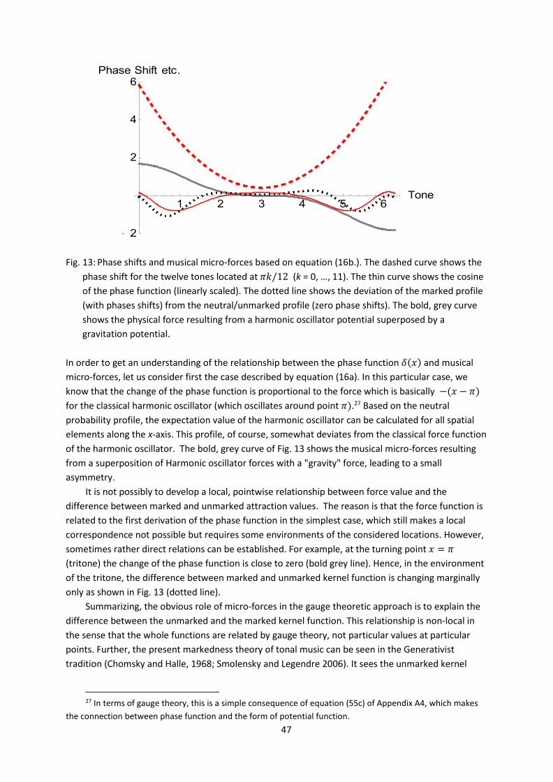
47

Fig. 13: Phase shifts and musical micro-forces based on equation (16b.). The dashed curve shows the

phase shift for the twelve tones located at 𝜋𝜋𝑘𝑘/12 (k = 0, …, 11). The thin curve shows the cosine of the phase function (linearly scaled). The dotted line shows the deviation of the marked profile (with phases shifts) from the neutral/unmarked profile (zero phase shifts). The bold, grey curve shows the physical force resulting from a harmonic oscillator potential superposed by a gravitation potential.

In order to get an understanding of the relationship between the phase function 𝛿𝛿(𝑥𝑥) and musical micro-forces, let us consider first the case described by equation (16a). In this particular case, we know that the change of the phase function is proportional to the force which is basically −(𝑥𝑥 − 𝜋𝜋) for the classical harmonic oscillator (which oscillates around point 𝜋𝜋).27 Based on the neutral probability profile, the expectation value of the harmonic oscillator can be calculated for all spatial elements along the x-axis. This profile, of course, somewhat deviates from the classical force function of the harmonic oscillator. The bold, grey curve of Fig. 13 shows the musical micro-forces resulting from a superposition of Harmonic oscillator forces with a "gravity" force, leading to a small asymmetry.

It is not possibly to develop a local, pointwise relationship between force value and the difference between marked and unmarked attraction values. The reason is that the force function is related to the first derivation of the phase function in the simplest case, which still makes a local correspondence not possible but requires some environments of the considered locations. However, sometimes rather direct relations can be established. For example, at the turning point 𝑥𝑥 = 𝜋𝜋 (tritone) the change of the phase function is close to zero (bold grey line). Hence, in the environment of the tritone, the difference between marked and unmarked kernel function is changing marginally only as shown in Fig. 13 (dotted line).

Summarizing, the obvious role of micro-forces in the gauge theoretic approach is to explain the difference between the unmarked and the marked kernel function. This relationship is non-local in the sense that the whole functions are related by gauge theory, not particular values at particular points. Further, the present markedness theory of tonal music can be seen in the Generativist tradition (Chomsky and Halle, 1968; Smolensky and Legendre 2006). It sees the unmarked kernel

27 In terms of gauge theory, this is a simple consequence of equation (55c) of Appendix A4, which makes

the connection between phase function and the form of potential function.

1 2 3 4 5 6Tone

2

2

4

6Phase Shift etc.

48

function as innate whereas the marked form is assumed to be developed under the pressure of learning.

6.2 The evolution of phase parameters by iterated learning: a case of self-organizing gauge fields Is there a deeper cognitive motivation for some of the descriptive frameworks that were developed to describe the peculiarities of tonal music? In order to answer this question we will look at an insightful paper by David Huron. Huron (2001) has derived several rules of voice-leading from perceptual principles that explain how the separation of different voices in a polyphonic piece of music can be optimized.28

In the present paper we are not concerned with voice leading but with static and dynamic attraction phenomena; the former ensuring the existence of tonal hierarchies, and the latter including rules of harmonic progression. Taken the inspiration from Huron (2001) and the grounding literature (Harnad, 1990; Sun, 2000), we could ask for a deeper cognitive motivation or grounding of the descriptive framework. The descriptive framework is the qubit quantum model which is crucially identified by fitting the phase parameters.

Music is made in the mind. It is the mind that structures the auditory sound stream into comprehensible music. There are particular properties of the mind that make the comprehension of music possible. I think Krumhansl, Lerdahl, Jackendoff and many others are right in assuming that tonal hierarchies play an essential role in this process of structure-building (see Section 4.1). Even when we acknowledge the essential role of tonal hierarchies for the basic tonal pitch space – as formulated by Lerdahl (1988) – this does not mean that we presume these hierarchies as innate, i.e. pre-existing and without the need of learning. Instead, the present claim is that there are mechanisms of routinization and knowledge reorganization that are decisive for forming these prerequisites. In Blutner (2007, 2010) I called the underlying mechanism fossilization. The core idea is borrowed from formal pragmatics (Morgan, 1978) and from theories of language change (e.g. Traugott, 1989; Traugott & Dasher, 2005).

I will use the term fossilization here in a very broad sense that covers the whole spectrum of the mentioned phenomena. It stands for processes of individual fossilization (sometimes called routinization) that take place in individual language acquisition, i.e. on a time scale of seconds, hours and months. What is more it stands for social processes of cultural fossilization that take place in language change on a historical time scale of years up to centuries; the relevant mechanism is iterated learning/cultural evolution. (Blutner, 2010)

In particular, I refer to ideas of self-organization in terms of iterated learning as developed in optimality theory (Tesar & Smolensky, 2000). The general learning method underlying this theory is reinforcement learning (Law & Gold, 2009; Sutton & Barto, 1998). The hope is that the hierarchies postulated in generative music theory can be derived from the general cognitive mechanism of self-organization (modelled in terms of iterated learning).

In optimality theory, iterated learning takes place dependent on the presentation of spoken inputs. The child first takes the role of a listener. It listens to the inputs, parses it in a certain way and then switches to the role of the speaker. Next, it generates an output from the given parse. Normally,

28 Huron (2001: 32) formulates the following "goal of voice-leading: G1. The goal of voice-leading is to

create two or more concurrent yet perceptually distinct 'parts' or 'voices.' Good voice-leading optimizes the auditory streaming."

49

the generated output and the given spoken input are not the same. The (relevant) difference between these two states is the reinforcement signal for correcting the underlying constraint system by adapting the weights. The general learning rule says: promote constraints that favour wanted behaviour over unwanted, demote constraints that favour unwanted behaviour over wanted. Hence, in case of a relevant difference, the weights of violated constraints are decreased (constraint demotion) and the weights of satisfied constraints are increased (constraint promotion), where only the perspective of the speaker counts.

In the case of tonal music, we have to adapt the basic idea of the OT bootstrapping/iterated learning mechanism. In the present musical context, there are agents who can play two different roles called Key and Tone. The role Key is to generate a key from one or several tones (corresponding to the role of the Listener in the natural language case). The role Tone is the opposite: to generate a plausible tone or sequence of tones that fits to the given key (corresponding to the role of the Speaker in the natural language case). If the initial tone(s) and the generated tone(s) agree, the system of constraints is not changed. If there is a discrepancy, the reinforcement mechanism comes into play.

The present situation is different from standard OT situation where the constraints are normally binary and not parameterized but absolute. In the present case, the constraints are graded function and they are parameterized by the phase parameters. This opens the possibility to modify the constraints by changing the values of their parameters. In order to get a quantitative theory of this change, the method of gradient descent has been used. In the simplest case, it has to maximize the difference 𝑃𝑃(𝑘𝑘/𝑘𝑘𝑒𝑒𝑦𝑦) − 𝑃𝑃(𝑘𝑘′/𝑘𝑘𝑒𝑒𝑦𝑦), where 𝑘𝑘 is the initial tone which triggers a particular key and 𝑘𝑘′ is the generated tone that fits this key. If 𝑘𝑘′ ≠ 𝑘𝑘, then the phase parameters that determine 𝑃𝑃(𝑘𝑘/𝑘𝑘𝑒𝑒𝑦𝑦) have to be adapted in order to increase the declared difference. This will result in the following learning rule:

(21) 𝑐𝑐ℎ𝑎𝑎𝑛𝑛𝑎𝑎𝑒𝑒 𝑐𝑐𝑜𝑜 ∆𝑘𝑘−𝑚𝑚 = −𝜂𝜂 ∙ 𝑠𝑠𝑖𝑖𝑛𝑛(∆𝑘𝑘−𝑚𝑚) ∙ cos (𝜋𝜋(𝑘𝑘 −𝑚𝑚) 6⁄ ), where 𝑚𝑚 𝜖𝜖 𝑘𝑘𝑒𝑒𝑦𝑦 and 𝜂𝜂 is a learning parameter

Summarizing, the proposed bootstrapping model is intended to ground the required parameters (phase factors) of the quantum model, which earlier were determined by data fitting. Instead, an algorithm for key-identification is constructed that automatically controls the system of free parameters and optimizes its own performance. The hope is that this algorithm explains the constitution of tonal hierarchies as stipulated by the mentioned authors. The algorithm starts with the neutral (unmarked) system of constraint functions exploiting the symmetry principle of

transposition invariance (ℤ12) augmented with a bootstrap mechanism of bidirectional learning. This device stepwise acquires the phase parameters that correspond to the assumption of tonal hierarchies. In other words, I argue for a machinery of deep gauge where the quantum field is iteratively gauged through an bootstrap mechanism of deep learning.

The first attempts to model the emergence of stabilizing phase shifts and with that a corresponding gauge field were succesful. Starting with the neutral kernel function, the system stabilized into a parameter set that approached the empirically determined kernel function presented in Section 5.3 (r = 0.82). More studies are required to investigatre the reliability of the bootstrapping mechanism and for improving the results by including more than one tone that is generated per step. The results of these studies will be reported independently.

50

7. General discussion and conclusions Structural and probabilistic approaches in computational music theory have tried to give systematic answers to the problem of tonal attraction. I have discussed two previous models of tonal attraction, one based on tonal hierarchies (Lerdahl 1988, 2001) and the other based on interval cycles (Woolhouse, 2009, 2010; Woolhouse & Cross, 2010). Both models aim to account for the phenomenon of tonal attraction at the level of pitches, regions, and chords. Unfortunately, both models have serious limitations. The hierarchical model has serious conceptual flaws because it stipulates the empirical generalisations rather than predicting them. Further, it envisages symmetric similarity relations between regions and chords, which cannot be correct empirically. The ICP-model, on the other hand, has interesting methodological advantages. Further, it is very successful empirically when the dynamics of attractions is considered. However, it fails for modelling static attraction potentials. To overcome the shortcomings of these models, I proposed a new probabilistic model relying on insights of quantum cognition. I have argued that the quantum approach integrates the insights from quantum symmetries and quantum probability theory.

The main advantages of the present quantum approach are both empirically and methodologically. Here is a shortlist of these advantages:

1. The quantum model integrates static and dynamic attraction profiles by fitting only one

parameter (a phase difference). 2. It draws a new light on multi-regression analysis quite popular in cognitive music theory (e.g.

Krumhansl; Huron 2008) by demonstrating its close connection to harmony theory. It further provides new insights of what are "adequate" constraint functions.

3. It introduces markedness theory into the domain of tonal music. Originally, the conception of markedness has been developed in generative linguistic and optimality theory. If the model's distinction between learned knowledge (described by phase parameters) and more or less innate knowledge (which is due to symmetry principles) contains a bit of truth, then ideas borrowed from quantum theory can realize important subjects of the generative tradition. Concerning the innateness issue, I do not see much wisdom in the generativist's stipulation of tonal hierarchies and ignoring matters of symmetry. Rather, I think that without a careful treatment of symmetry principles – such as the principle of translation invariance – a cognitive theory of tonal music is not possible (Balzano, 1980; Honingh, 2006; Mazzola, 2002).

4. A surprising outcome of this paper is that we can make a judgment on the percentage of variance that comes from the symmetry conserving quantum model (and possibly can be seen as innate and not learnable) and that part of the quantum model that deals with symmetry breaking and fixing the phases. The first part of the variance is about 50%, the second part is about 40% and 10% cannot be explained.

5. The guide of a lattice gauge field opens a new way to understand musical micro-forces as instruments that modify and transform neutral/unmarked attraction kernels into actual (marked) kernels that describe real static and dynamic attraction profiles. Note that in third generation neural networks (spiking networks; cf. Vassilieva, Pinto, Acacio de Barros, & Suppes, 2011) it is plausible to take the phases of the oscillations into account. This introduces elements that are at a lower level of decription than provided by the standard symbolic frameworks. For that reason we use the term "micro-forces".

6. In quantum cognition, several authors have made use of field-theoretic ideas. To mention only the top of the iceberg, I will refer to the modelling of complex concepts (Aerts, 2007),

51

minimalism in generative linguistics (beim Graben & Gehrt, 2012; Piattelli-Palmarini & Vitiello, 2015), and models of the financial market (e.g., Bagarello & Haven, 2015). However, most of these models only exploit the power of Fock-space representation to model complex entities. The present approach is the first one that exploits the heart of quantum field theory: symmetries and gauge fields.

7. Another important issue is the implementation of self-organizing processes in order to restrict the stipulated phase shifts for the diachronic scale. Considering the role of the phase shifts for fixing the lattice gauge field, we can see this as modelling the emergence of gauge fields by a mechanism of iterated learning. Hence, I am arguing for a deep gauge where the quantum field is iteratively gauged through an evolutionary mechanism of deep learning, similar to bidirectional optimality theory in cognitive linguistics.

It goes not without mentioning that the present model is far from being complete. The present model is concentrated on static and dynamic attraction phenomena. Static attraction phenomena are connected with ensuring the existence of tonal hierarchies. Dynamic attraction phenomena include melodic implications and the motivation of harmonic progression rules. Hence, we were not concerned with voice leading (cf. Huron 2001), i.e. with mechanisms that separate different voices of a musical stream. Further, the present model does not incorporate information that listeners infer from longer temporal sequences. According to Lerdahl (1988), these are the effects of event hierarchies, which deserve a special treatment – possibly along the lines of Mazzola (Mazzola, 2002; Mazzola et al., 1989), or Schenker (1935) and Marsden (2010) . The dynamics of attraction, thus, was restricted to the simplest possible cases exemplified by the mentioned studies of Povel, Larson, Woolhouse, and others. Further, in the present literature of explaining tonal attraction, the spectral pitch class model (Milne et al., 2015) plays an essential role. In this model, the pitch perception of any musical sound is described by using spectral pitch class vectors. There are close relationships between this Helmholtzian model (Helmholtz, 1877) and the present quantum approach which should be pursued in a later publication.

What is the precise connection between the two conceptions of forces that underlies the present enterprise: phenomenological forces and micro-forces? As I made clear in Section 4.5, phenomenological forces are established within a metaphoric theory of musical movements, for example as developed in Larson's theory of musical forces. This sharply contrast with the introduction of tonal micro-forces in Section 6. In both cases, the forces can be formulated in terms of binary/graded constraint functions. However, it was not possible to establish systematic relations between both types of constraints functions.29 This invites the idea to both types of forces could be seen as complementary, living on different levels of representation. Hence, the phenomenological forces discussed in folk theories of music are at a different level of representation than tonal micro-forces as organized by lattice gauge fields.

Another issue concerns the issue of transposition invariance. Of course, it is an empirical question whether there are significant differences between different keys. Legendary authors such as Helmholtz (1877) have doubt such differences. Others have vehemently argued for them, e.g. Beckh (1937). In the present model, symmetry breaking can introduce significant differences between the various keys. We have eliminated this kind of symmetry violation by a simple trick resetting the tonic

29 We made several attempts to correlate constraints such as gravity, magnetism, relative attraction,

proximity, closure, registral return, etc. with the constraints resulting from the tonal micro-forces. Unfortunately, these attempts did not lead to a clear outcome.

52

to a fixed value and considering intervals based on the tonic. At the moment, it is not clear whether there is independent motivation for the "trick". We have to leave this issue unresolved here.

In his seminal book, Meyer (1956) pointed out that the principal emotional content of music arises through the composer’s arranging of expectations. Composers sometimes satisfy our expectations, sometimes delay an expected outcome or even thwart it, and sometimes composers play with ambiguities avoiding any clear expectations to be established. The mathematical treatment of expectations is in terms of probabilities, let it be classical Bayesian probabilities (Oaksford & Chater, 2007; Temperley, 2007) or non-classical quantum probabilities (Busemeyer & Bruza, 2012). In this paper, I have investigated the problem of tonal attraction and I have argued for a probabilistic approach in terms of quantum probabilities. In this way, I have presented a framework for expressing and handling expectations. Looking at future work, this could be one of the building blocks for realising the mapping between music and its affective (emotional) answer. Another building block relevant for realizing the ultimate aim of connecting musical structures with affective meaning is the proper characterization of the qualitative character of chords in terms of consonance and dissonance.

A very naïve understanding of the composition process is that it is nothing else than looking for the most probable continuation of a starting sequence of tones. Of course, this is simply to realize with the help of neural networks. A composer normally aims to generate emotions in the mind of the listener. Emotions are deeply connected with subjective expectancy (Meyer 1956). However, it is crucially surprise that generates greet musical effects. Hence, the process of composition cannot be described as a mechanism for finding the most probable continuation. If one insists to see the process of composing as an optimization mechanism, then one has to considering higher rules of optimization. These rules are directed to resolving conflicting aims in following particular emotional goals, optimally separating different voices and, at the same time, pursuing certain restrictions of a particular style.

I will end with a very general remark concerning the sociology of sciences. Recently, some authors such as Rens Bod (Bod, 2014) have argued that the widely accepted opposition between the sciences (mathematical, experimental) and the Humanities is a serious mistake. There is a broad spectrum of examples that illustrate how ideas of the Humanities have made progress in sciences such as physics and mathematics still possible. The thinking about tonal music and its meaning, the construction of theories concerning the biological and social nature of music, and the role of simulating emotions by the performance of music played an important particularly puzzling role in the history of sciences. Hermann von Helmholtz, Hermann Rudolf Lotze, and his prodigious scholar Carl Stumpf demonstrate the close connections and interactions between sciences and Humanities in the field of music. Likely ideas from quantum cognition are welcome to intensify the enterprise.

Acknowledgement This paper is devoted to the memory of Remko Scha, physicist, computational linguist, composer and founder of the Institute of Artificial Art in Amsterdam, who died on November 9, 2015. The last time I met Remko was in summer 2015 in Berlin. We visited Schloß Niederschönhausen in Pankow (where Remko was overwhelmed by Wilhelm Pieck's self-made desk). At this occasion we also discussed about deep learning, musical forces and quantum cognition. It was Remko who came up with the idea of "deep gauge". I was always impressed by his gentle and sympathetic character. I am very grateful to a cherished and beautiful mind.

53

I thank Peter beim Graben for extensive discussions particularly regarding quantum field theory and applications in philosophy and cognitive science. Further, I would like to thank M. Woolhouse, J. Myers, and A. Milne for useful email exchange. The usual clause applies that any errors are my own and should not tarnish the reputations of these esteemed persons.

Appendix: Mathematical Basics of Quantum Theory

A1 Qubit states In classical information science, a bit is the basic unit of information in computation referring to a choice between two discrete states, say {0, 1}. In contrast, a qubit is the basic of information in quantum computing referring to a choice between two orthogonal unit-vectors in a two-dimensional

Hilbert space. For instance, the orthogonal states ϕ→ = (10) and ϕ↑ = (0

1) can be taken to represent

true and false, the vectors in between are appropriate for modeling degrees of truth (vagueness) or degrees of expectation (probabilities).

The simplest non-trivial physical system is a two state system, also called a qubit system. In such a system, each proper observable has exactly two (orthogonal) eigenvectors, say ϕ→ and ϕ↑. In the eigenstates of the observable the question asked by the observable has a certain outcome. Of course, a qubit can realize an infinite set of states but only two orthogonal states relate to eigenstates of the observable.

Formally, an arbitrary state of a qubit can be written as

(22) ψ = α ϕ↑+ β ϕ→ with α2 + β2 = 1

Making use of a particular parameterization of the states ψ every state of a qubit can be realized as the point on a three-dimensional sphere, the so-called Bloch sphere (Fig. 13, left hand side).

(23) ψ = cos(θ/2) ϕ↑ + sin(θ/2) e+i∆ ϕ→

The parameters θ and ∆ are nothing but spherical polar coordinates, 0 ≤ ∆ < 2π and 0 ≤ θ < π.30 One example of the realization of qubits is the spin of electrons. Hereby, it is possible to measure the spin in three "spatial" directions x, y and z. Another example is the polarization of photons. Hereby the state ϕ↑ represents a state with definite polarization in↑-direction; the state

21 (ϕ↑ − ϕ→)

represents definite polarization in ↖-direction; the superposition of states including a π/2 phase shift, such as

21 (ϕ↑ − i ϕ→), represents circularly polarized light.

30 That means we can represent each unit vector ψ as a point on the unit sphere in the three dimensional

space by the coordinates x = sin(θ) cos(∆), y = sin(θ) sin(∆), z = cos(θ). If the phase parameter ∆ is zero, then the y-component vanishes and the three-dimensional phase can be reduced to a circle in the x,z- plane with the coordinates x = sin(θ) and z = cos(θ). Note that the angle θ in the Bloch sphere corresponds to the angle θ/2 in the original parameterization (18). Hence, two orthogonal vector states correspond to opposite points on the Bloch sphere.

54

Fig. 14: Bloch sphere. Using equation (18) an arbitrary (normalized) state of the two-dimensional

Hilbert space can be parameterized by the two spherical polar coordinates θ and ∆. Hereby, ∆ corresponds to a phase shift of the two superposing states ϕ↑ and ϕ→ . On the right hand side, a "Bloch circle" is shown resulting from the assumption of a zero phase shift (∆ = 0).

For a simple illustration, consider a photon in a qubit state ψ, and take ϕ↑ as indicating vertical polarization and ϕ→ as indicating horizontal polarization. Then the probability that the object is vertically polarized (i.e. it collapses into the state ϕ↑) is

(24) P↑ (ψ) = |ϕ↑ ⋅ ψ|2 = cos2(θ/2) = ½(1+cos(θ))

Further, we can also calculate the probability that the object is polarized into a direction given by the superposition of ϕ↑ and ϕ→, say ↖ =

21 (ϕ↑ − ϕ→). Interestingly, if the photon is described by ψ and

collapses into the state ϕ↖, then the calculated probabilities for the collapse also depend on the phase shift ∆:

(25) P↖ (ψ) = ½ |(ϕ↑ − ϕ→) ⋅ ψ|2 = ½ (1 + cos(θ)⋅sin(∆/2)) For the understanding of quantum cognition, it is not required to give an interpretation in terms of some mysterious properties relating to the spin of electrons, the polarization of photons or other entities. In contrast to quantum mind theory (Hameroff & Penrose, 1995), quantum cognition does not follow strategies of reducing mental entities to physical ones. Not unlike representatives of artificial intelligence who try to analyse big corpora using vector states modelling their distributive semantics (Widdows, 2004), representatives of quantum cognition also work with vector states. The role of projections and quantum probabilities is essential in both cases.

Before we can apply the projection of states in order to calculate (probabilistic) attraction profiles, we have to introduce some basic ideas for symmetry groups.

55

A2 Group theory Here is a concise introduction of some basic concepts of group theory.31 Generally, a group consists of a set of (abstract) elements and a binary operation defined on it. Usually, this operation is written with a product sign, for example g1 ⋅ g2 ∈ G (the product sign „⋅“ can be left out). The following properties have to be satisfied:

1. All elements of G are connected by the group operation, i.e., for all elements g1, g2 ∈ G it holds

that g1 ⋅ g2 ∈ G 2. There is a particular element e ∈ G (the neutral element) such that for all elements g∈G it holds

that e ⋅ g = g ⋅ e = g. 3. The associative law is valid, i.e. for all elements g1, g2, g3 ∈ G we have (g1 ⋅ g2) ⋅ g3 = g1 ⋅ (g2 ⋅ g3). 4. For each element g∈G there exists an inverse element g−1, which has the property g ⋅ g−1 = g−1 ⋅ g

= e.

A group G is called cyclic if there exists a single element g ∈ G such that every element in G can be represented as a composition of g's. The element g is called a generator of the group. If a cyclic

group has n elements (i.e. the group is of order n), the group can be represented as ℤn = {e, g, g2,

g3, …, gn-1}, where gn= e. The general rule is that the generators for a cyclic group ℤn are exactly the numbers i in the range 0<i<n such that n and i are relatively prime (i.e., they have no common factor differently from 1).

A3 Schrödinger equation In his famous treatise, John von Neumann makes the distinction between "two fundamentally different types of interventions which can occur in a system" (von Neumann, 1932: p. 151). First, there are "the arbitrary changes by measurements" which result in a mixture of eigenstates of the measured observable, and, second, there are the automatic changes which occur with passage of time and which are described by the Schrödinger equation. The two kinds of interventions are also called type 1 and type 2 processes.

The Schrödinger equation gives a concise description of the temporal development of a quantum state Ψ. It can be stated as follows:

(26) 𝜕𝜕𝜕𝜕𝑖𝑖ψ(𝑥𝑥, 𝑡𝑡) = −𝑖𝑖𝐻𝐻ψ(𝑥𝑥, 𝑡𝑡)

Here is a simple example of the Schrödinger equation applied to the psychological phenomenon of bistable perception. The phenomenon arises in situation where two possible interpretations of a target input appear and a kind of oscillation takes places between the two interpretations. Using the instruments of quantum cognition, the phenomenon was first investigated in the domain of logical paradoxes (Aerts, Broekaert, & Smets, 1999). A so-called liar sentence says of itself that it is wrong. The logic of such sentences involves a self-referential circularity, and it encompasses a truth-value oscillation which can be modelled in the framework of quantum theory. The phenomenon of bistable perception was also investigated in connection with the Necker tube figure (Atmanspacher, Filk, & Römer, 2004). My presentation does not directly follow the original papers. Instead, I follow the

31 For the interested reader, we refer to standard textbooks of group theory (Alexandroff, 2012; Jones,

1998) or good introductory sections or appendixes in music-theoretic treatises (Balzano, 1980; Honingh, 2006)

56

presentation developed in chapter 8.1 of Busemeyer and Bruza (2012). This presentation illuminates the close connection with Markov models. Fig. 15: Two-state transition graph for bistable perception For the mathematical treatment, we consider a discrete state space {A, B} and a stochastic process {𝑋𝑋(𝑡𝑡)}𝑖𝑖≥0 consisting of a system of random variables X(t) relative to our discrete state space. Further,

we assume probability vectors (𝑃𝑃(𝑋𝑋(𝑡𝑡) = 𝐴𝐴𝑃𝑃(𝑋𝑋(𝑡𝑡) = 𝐵𝐵). These vectors are related to the corresponding

vectors at other times by a linear transformation T which depends of the time difference only:

(27) (𝑃𝑃(𝑋𝑋(𝑡𝑡′) = 𝐴𝐴𝑃𝑃(𝑋𝑋(𝑡𝑡′) = 𝐵𝐵) = 𝑇𝑇(𝑡𝑡′ − 𝑡𝑡) (𝑃𝑃(𝑋𝑋(𝑡𝑡) = 𝐴𝐴

𝑃𝑃(𝑋𝑋(𝑡𝑡) = 𝐵𝐵)

Further, we stipulate a condition, which is called the semi-group property of dynamic systems: (28) 𝑇𝑇(𝑢𝑢 + 𝑣𝑣) = 𝑇𝑇(𝑢𝑢) ∙ 𝑇𝑇(𝑣𝑣) = 𝑇𝑇(𝑣𝑣) ∙ 𝑇𝑇(𝑢𝑢) If we make some plausible assumptions, for instance that in the limit of a zero time differences, the unit matrix 1 is approximated ( lim

∆𝑖𝑖→0𝑇𝑇(∆𝑡𝑡) = 1), then we can derive the following differential equation

which is called the Kolmogorov forward equation with the 2x2 intensity matrix K:32

(29) 𝑑𝑑𝑇𝑇(𝑖𝑖)𝑑𝑑𝑖𝑖

= 𝐾𝐾 ∙ 𝑇𝑇(𝑡𝑡)

In terms of the transition parameters α and β depictured in Fig. 14, the matrix K can be written as follows:

(30) 𝐾𝐾 = (−𝛽𝛽 𝛼𝛼𝛽𝛽 −𝛼𝛼)

The solution to equation (29) is the matrix exponential function:33 (31) 𝑇𝑇(𝑡𝑡) = 𝑒𝑒𝑖𝑖𝑡𝑡

32 For an explanation of the mathematical details the reader is referred to standard textbooks of

stochastic processes, for instance van Kampen (1992) or Bhattacharya and Waymire (1990) 33 The definition of the matrix exponential is 𝑒𝑒𝑀𝑀 = lim

𝑖𝑖→∞

1𝑖𝑖!𝑀𝑀𝑖𝑖, where M is a 2x2 matrix and the exponential

𝑀𝑀𝑖𝑖+1 is recursively defined by the matrix product 𝑀𝑀𝑖𝑖 ∙ 𝑀𝑀.

57

Assuming at t=0 the system is in the state A, implicates the initial vector (10) of response

probabilities. Using equation (31), this vector is transformed into a probability vector 𝑒𝑒𝑖𝑖𝑡𝑡 (10)

reflecting the probabilities of the two states at time t. If α > β, the system tends to stay in state A (with a probability bigger than ½). If α < β, then the system tends to transit to state B (with a prob-ability bigger than ½). If we start with a mixed state where A and B are equally probable, then for α > β the system transits to state A with a probability bigger than ½. In contrast, for α < β, the system transits to state B with a probability bigger than ½. If α = β, then the probabilistic situation is not changed. Fig. 16 shows the probability resulting for state A at time t for different values of 𝛼𝛼 and 𝛽𝛽.

Fig. 16: Transition probabilities for different values of α and β for the Markov model. On the left

hand, the system is initially (t = 0) in state A with probability 1; on the right hand side initially both states are equally probable.

Now we consider the two-dimensional quantum model of bistable perception. Again, we assume (as depictured in Fig. 15) that the bistable system can be in one of two states. However, in the quantum

model we model these two states by the orthogonal states ψ→ = (10) and ψ↑ = (0

1) of a single qubit

system. The quantum process starts at time t = 0 in a superposition of these two states ψ (0) = a ψ→ + b ψ↑, with real number a and b, a2+b2 = 1. If a = 1 (and b = 0) then the system starts in the state we earlier have labelled by A. In contrast to the Markov model where we directly consider probability vectors, in the quantum model we are confronted with probability amplitudes ψ(t) for each point of time t. The probability for the two events A or B ‒ described by the two base vectors ψ→ and ψ↑, respectively ‒ conforms to the squared length of the scalar product between the probability amplitudes ψ(𝑡𝑡) and the corresponding base vector. In quantum theory, the transition from one quantum state to another one is described by a unitary transformation (in order to preserve lengths and inner products), which is a direct function of the time difference between initial and final states: (32) ψ(𝑡𝑡′) = 𝑈𝑈(𝑡𝑡′ − 𝑡𝑡)ψ(𝑡𝑡)

Further, as in the Markov case, the semi-group property is assumed:

1 2 3 4Time

0.2

0.4

0.6

0.8

Probability α β 2 .2 .9 .2 .5 .2 .2 .2 .2 .5 .2 .9 .2 2

58

(33) 𝑈𝑈(𝑢𝑢 + 𝑣𝑣) = 𝑈𝑈(𝑢𝑢) ∙ 𝑈𝑈(𝑣𝑣) = 𝑈𝑈(𝑣𝑣) ∙ 𝑈𝑈(𝑢𝑢) From this condition the following differential equation can be derived, which is called the Schrödinger equation for the unitary development of U:

(34) 𝑑𝑑𝑑𝑑𝑖𝑖𝑈𝑈(𝑡𝑡) = −𝑖𝑖 ∙ 𝐻𝐻 ∙ 𝑈𝑈(𝑡𝑡)

The 2x2 matrix H is the pendent to the intensity matrix in the Markov forward equation (29). It must be Hermitian to guarantee that the solution of equation (34) is unitary34. From equation (34) it is straightforward to derive the Schrödinger equation (26) as an equation for the temporal development of the quantum state ψ(𝑡𝑡). It is repeated here:

(35) 𝑑𝑑𝑑𝑑𝑖𝑖ψ(𝑡𝑡) = −𝑖𝑖𝐻𝐻ψ(𝑡𝑡).35

In the simplest case, the Hamilton operator giving rise to transitions of the system can be written in as

(36) 𝐻𝐻 = ℎ 𝜎𝜎𝑛𝑛 = ℎ (0 11 0)

where 𝜎𝜎𝑛𝑛 is the first Pauli spin operator and ℎ is a coupling constant.36 The general form of the unitary matrix for a given Hamiltonian equals 𝑈𝑈(𝑡𝑡) = 𝑒𝑒−𝑖𝑖𝑖𝑖𝐻𝐻. Taking the Hamiltonian from equation (31), the unitary operator of time evolution is

(37) 𝑈𝑈(𝑡𝑡) = ( cos(ℎ𝑡𝑡) −𝑖𝑖 𝑠𝑠𝑖𝑖𝑛𝑛(ℎ𝑡𝑡)−𝑖𝑖 𝑠𝑠𝑖𝑖𝑛𝑛(ℎ𝑡𝑡) cos(ℎ𝑡𝑡) )

Taken the initial state is ψ(0) = ψ→ (i.e., the system is initially in state A), then we can derive the following probability that the system is still in state A at time t: (38) ‖ψ(𝑡𝑡) ∙ ψ→‖2 = 𝑐𝑐𝑐𝑐𝑠𝑠2ℎ𝑡𝑡

Hence, the quantum model predicts an oscillation between the two states with a frequency depending of the coupling constant. This contrast sharply with the classical Markov model that does not predict such a switching behaviour. There is another important consequence of the quantum model that was pointed out by Atmanspacher, Filk, & Römer (2004). These authors investigated how measurements of the response state can influence the response probabilities. The prediction of the

34 The factor i is crucial for ensuring that H is Hermitian. Without this factor, we are concerned with an

anti-Hermitian Hamiltonian operator. 35 As in the Markov case, it is assumed that H is not explicitly time-dependent. This makes sure that the

solutions of the Schrödinger equation are the so-called "stationary solutions". 36 Note that Busemeyer and Bruza (2012) propose a more general form for the Hamiltonian with two

(real-valued) parameters.

59

model was (making crucial use of the projection postulate of measurements) that an increased number of observations decreases the probability that the system will switch. In the limit of decreasing the observation interval toward zero this has the effect that the time we have to wait to see a change of the state increases infinitely (quantum Zeno effect). There are interesting empirical findings that support the model (Atmanspacher & Filk, 2010; Yearsley & Pothos, 2016).

A4 Gauge invariance Assume a physical system is invariant with respect to some global (i.e., independent of space and time) group of continuous transformations. Then the idea of gauge invariance, is to make the stronger assumption that the basic physical equations describing the system have to be invariant when the group operations are considered locally (i,e, dependent on time and the other coordinates of the system). Normally, this principle of gauge invariance, leads to a modification of the original equation and introduces additional terms which can be interpreted as new "forces" induced by the "gauge field", which describes this local dependencies.

The idea of gauge invariance was first developed by Hermann Weyl in 1918, when he made the attempt to unify gravity and electromagnetism. Weyl assumed that the length of any single vector is arbitrary. Only the relative lengths of any two vectors and the angle between them are preserved under parallel transport. This was the birth of a new idea in physics which was called "gauge invariance" by Weyl. Even when Weyl's attempt to develop a unified theory failed, the idea survived and was extremely successful later on. In my opinion, it is this success that justifies the theory. The theory itself remains mysterious to a certain degree: we do not have an independent, physical or methodological motivation for it.

In quantum physics, the idea of gauge symmetry was applied much later by Schrödinger, Klein, Fock and others (for an overview, see Jackson & Okun, 2001). We know that all changes of the quantum state by a global phase factor leave all observable physical effects unchanged. This can be called a global phase symmetry. Such a global phase change can be described by the transformation (39) ψ(𝑥𝑥, 𝑡𝑡) ⟶ψ(𝑥𝑥, 𝑡𝑡) 𝑒𝑒𝑖𝑖δ Here, 𝛿𝛿 is a phase parameter (independent of x and t). In agreement with the ghost of gauge invariance, let us postulate now that there is a bigger symmetry: local phase symmetry. It leaves all observable effects invariant when local phase transformations are applied: (40) ψ(𝑥𝑥, 𝑡𝑡) ⟶ψ(𝑥𝑥, 𝑡𝑡) 𝑒𝑒𝑖𝑖𝛿𝛿(𝑛𝑛,𝑖𝑖)

The idea now is to assume that local phase symmetry is the gauge symmetry that we have to assume in quantum physics. It is not difficult to see that the Schrödinger equation (26) is not invariant by local phase transformations. However, it is invariant when a simultaneous transformation of the Hamiltonian is carried out by adding a fixed potential function

(41) 𝐻𝐻 ⟶𝐻𝐻− 𝜕𝜕𝜕𝜕𝑖𝑖

(𝑥𝑥, 𝑡𝑡)

Let us check the invariance of the Schrödinger equation when performing the simultaneous transformations (40) and (41) under the simplifying assumption that the Hamiltonian H does not

60

affect the local coordinates. After applying equation (40), the left hand side of the Schrödinger

equation (26) is the expression 𝜕𝜕𝜕𝜕𝑖𝑖ψ(𝑥𝑥, 𝑡𝑡)𝑒𝑒𝑖𝑖𝛿𝛿(𝑛𝑛,𝑖𝑖). For this expression we get the equivalence

(42) 𝜕𝜕𝜕𝜕𝑖𝑖ψ(𝑥𝑥, 𝑡𝑡)𝑒𝑒𝑖𝑖𝛿𝛿(𝑛𝑛,𝑖𝑖) = 𝑖𝑖ψ(𝑥𝑥, 𝑡𝑡)𝑒𝑒𝑖𝑖𝛿𝛿(𝑛𝑛,𝑖𝑖) 𝜕𝜕

𝜕𝜕𝑖𝑖𝛿𝛿(𝑥𝑥, 𝑡𝑡) + 𝑒𝑒𝑖𝑖𝛿𝛿(𝑛𝑛,𝑖𝑖) 𝜕𝜕

𝜕𝜕𝑖𝑖ψ(𝑥𝑥, 𝑡𝑡).

On the other hand, after applying the transformations (40) and (41), for the right hand side of (26) we get the equivalence

(43) −𝑖𝑖𝐻𝐻ψ(𝑥𝑥, 𝑡𝑡)𝑒𝑒𝑖𝑖𝛿𝛿(𝑛𝑛,𝑖𝑖) + 𝑖𝑖ψ(𝑥𝑥, 𝑡𝑡)𝑒𝑒𝑖𝑖𝛿𝛿(𝑛𝑛,𝑖𝑖) 𝜕𝜕𝜕𝜕𝑖𝑖𝛿𝛿(𝑥𝑥, 𝑡𝑡) = 𝑖𝑖ψ(𝑥𝑥, 𝑡𝑡)𝑒𝑒𝑖𝑖𝛿𝛿(𝑛𝑛,𝑖𝑖) 𝜕𝜕

𝜕𝜕𝑖𝑖𝛿𝛿(𝑥𝑥, 𝑡𝑡) − 𝑖𝑖𝑒𝑒𝑖𝑖𝛿𝛿(𝑛𝑛,𝑖𝑖)𝐻𝐻ψ(𝑥𝑥, 𝑡𝑡)

Assuming the validity of the (untransformed) Schrödinger equation (26), we can see that both sites are equivalent.

Next, let us consider an example where the operator H affects a local coordinate. I consider a

free particle moving in one dimension x. In this case, the Hamiltonian is 𝐻𝐻 = 𝑝𝑝2

2𝑚𝑚. It describes the

kinetic energy of the particle of mass m and momentum p. In quantum theory, the momentum

corresponds to an operator −𝑖𝑖ℏ 𝜕𝜕𝜕𝜕𝑛𝑛

, where ℏ is Planck's quantum of angular momentum. In the

present, non-physical context, hence we can consider a modification of the general form of the Schrödinger equation (26), for describing objects in space and time:

(44) 𝜕𝜕𝜕𝜕𝑖𝑖ψ(𝑥𝑥, 𝑡𝑡) = −𝑖𝑖 𝑐𝑐𝑐𝑐 𝜕𝜕

2ψ(𝑛𝑛,𝑖𝑖)𝜕𝜕𝑛𝑛2

,

with a real number constant cc.37 The solution of this equation is a plane wave and their superpositions: (45) ψ(𝑥𝑥, 𝑡𝑡) = 𝐴𝐴𝑒𝑒−𝑖𝑖(𝑖𝑖𝑖𝑖±𝑛𝑛𝑛𝑛),

where A denotes a complex amplitude. The wave number n and circular frequency 𝜔𝜔 are related through the dispersion equation

(46) 𝜔𝜔 = 𝑐𝑐𝑐𝑐 ∙ 𝑛𝑛2 . The final solution of the Schrödinger equation must obey the given initial and boundary conditions. As initial condition we may set ψ(0,0) = 1 for encoding the tonal context. Additionally we have periodic boundary conditions on the unit circle ψ(𝑥𝑥 + 4𝜋𝜋, 𝑡𝑡) = ψ(𝑥𝑥, 𝑡𝑡). The former yields A = 1, while

the latter gives a quantization constraint e4πin = 1, and hence n should be 1/2, 3/2, 5/2. Choosing the

fundamental wave number n = 1/2 yields ω = 𝑐𝑐𝑐𝑐/4. Finally, the superposition of the fundamental solutions 𝑒𝑒+𝑖𝑖(𝑛𝑛𝑛𝑛−𝑖𝑖𝑖𝑖)and 𝑒𝑒−𝑖𝑖(𝑛𝑛𝑛𝑛−𝑖𝑖𝑖𝑖) for n = ½ gives

(47) ψ(𝑥𝑥, 𝑡𝑡) = 𝑒𝑒−𝑖𝑖𝑖𝑖𝑖𝑖cos(𝑥𝑥/2)

37 Obviously, in quantum mechanics of a particle with mass m, the parameter cc is identical with ℏ

2𝑚𝑚.

61

which is a standing wave along the unit circle with probability density |ψ(x, t)|2

= cos2(x/2). For

describing tonal music with 12 tones we need a discretization of the feature space which we can

achieve through sampling 𝑥𝑥𝑘𝑘 = 𝜋𝜋𝑘𝑘6

, for k∈{0, 1, …, 11}. The unmarked default distribution is then as

follows:

(48) 𝑝𝑝𝑘𝑘 = cos2(𝜋𝜋𝑘𝑘12

).

This agrees with the neutral case discussed in Section 5.2.

For a local gauge transformation (40), things become more involved when a space-dependence of the Hamiltonian as in the Schrödinger equation in the form of equation (44) is considered. For the temporal derivative we obtain equation (42), as discussed before. It can be rewritten in the following form:

(49) 𝜕𝜕𝜕𝜕𝑖𝑖ψ(𝑥𝑥, 𝑡𝑡)𝑒𝑒𝑖𝑖𝛿𝛿(𝑛𝑛,𝑖𝑖) = 𝑒𝑒𝑖𝑖𝛿𝛿(𝑛𝑛,𝑖𝑖)( 𝜕𝜕

𝜕𝜕𝑖𝑖+ 𝑖𝑖 𝜕𝜕𝛿𝛿(𝑛𝑛,𝑖𝑖)

𝜕𝜕𝑖𝑖)ψ(𝑥𝑥, 𝑡𝑡)

Likewise, we can calculate the spatial derivative on the right hand site of equation (44). It yields the following Laplacian:

(50) 𝜕𝜕2

𝜕𝜕𝑛𝑛2ψ(𝑥𝑥, 𝑡𝑡)𝑒𝑒𝑖𝑖𝛿𝛿(𝑛𝑛,𝑖𝑖) = 𝑒𝑒𝑖𝑖𝛿𝛿(𝑛𝑛,𝑖𝑖)( 𝜕𝜕

𝜕𝜕𝑛𝑛+ 𝑖𝑖 𝜕𝜕𝛿𝛿(𝑛𝑛,𝑖𝑖)

𝜕𝜕𝑛𝑛)2ψ(𝑥𝑥, 𝑡𝑡)

It is usual to introduce a special notion for the operators in round brackets, which are called covariant derivatives:

(51) a. Dt =𝜕𝜕𝜕𝜕𝑖𝑖

+ 𝑖𝑖 𝜕𝜕𝛿𝛿(𝑛𝑛,𝑖𝑖)𝜕𝜕𝑖𝑖

b. Dx =𝜕𝜕𝜕𝜕𝑛𝑛

+ 𝑖𝑖 𝜕𝜕𝛿𝛿(𝑛𝑛,𝑖𝑖)𝜕𝜕𝑛𝑛

The phase function 𝛿𝛿(𝑥𝑥, 𝑡𝑡) is called gauge field. Using covariant derivations instead of the conventional ones renders the Schrödinger equation (44) locally gauge invariant:

(52) 𝐷𝐷𝑖𝑖ψ(𝑥𝑥, 𝑡𝑡) = −𝑖𝑖 𝑐𝑐𝑐𝑐 𝐷𝐷𝑛𝑛2ψ(𝑥𝑥, 𝑡𝑡)

Next, we consider an important simplification and assume that the gauge does not explicitly depend

on time, i.e. 𝜕𝜕𝛿𝛿(𝑛𝑛,𝑖𝑖)𝜕𝜕𝑖𝑖

= 0. Then the covariant Schrödinger equation reads

(53) 𝜕𝜕𝜕𝜕𝑖𝑖ψ(𝑥𝑥, 𝑡𝑡) = −𝑖𝑖 𝑐𝑐𝑐𝑐 ( 𝜕𝜕

𝜕𝜕𝑛𝑛+ 𝑖𝑖 𝜕𝜕𝛿𝛿(𝑛𝑛,𝑖𝑖)

𝜕𝜕𝑛𝑛)2ψ(𝑥𝑥, 𝑡𝑡)

Evaluating the spatial derivative yields

(54) ( 𝜕𝜕𝜕𝜕𝑛𝑛

+ 𝑖𝑖 𝜕𝜕𝛿𝛿(𝑛𝑛,𝑖𝑖)𝜕𝜕𝑛𝑛

)2ψ(𝑥𝑥, 𝑡𝑡) = 𝜕𝜕2

𝜕𝜕𝑛𝑛2ψ(𝑥𝑥, 𝑡𝑡) + (𝜕𝜕𝛿𝛿(𝑛𝑛,𝑖𝑖)

𝜕𝜕𝑛𝑛𝜕𝜕𝜕𝜕𝑛𝑛

+ 12𝜕𝜕2𝛿𝛿(𝑛𝑛,𝑖𝑖)𝜕𝜕𝑛𝑛2

)ψ(𝑥𝑥, 𝑡𝑡) + (𝜕𝜕𝛿𝛿(𝑛𝑛,𝑖𝑖)𝜕𝜕𝑛𝑛

)2ψ(𝑥𝑥, 𝑡𝑡)

such that the gauged Hamiltonian in the Schrödinger equation 𝜕𝜕𝜕𝜕𝑖𝑖ψ(𝑥𝑥, 𝑡𝑡) = −𝑖𝑖 𝐻𝐻ψ(𝑥𝑥, 𝑡𝑡) becomes a

sum of three operators.

62

(55) 𝐻𝐻 = 𝑇𝑇 + 𝑀𝑀 + 𝑈𝑈 with

a. 𝑇𝑇 = −𝑐𝑐𝑐𝑐 𝜕𝜕2

𝜕𝜕𝑛𝑛2

b. 𝑀𝑀 = −2𝑖𝑖 ∙ 𝑐𝑐𝑐𝑐 (𝜕𝜕𝛿𝛿(𝑛𝑛,𝑖𝑖)𝜕𝜕𝑛𝑛

𝜕𝜕𝜕𝜕𝑛𝑛

+ 12𝜕𝜕2𝛿𝛿(𝑛𝑛,𝑖𝑖)𝜕𝜕𝑛𝑛2

)

c. 𝑈𝑈 = 𝑐𝑐𝑐𝑐(𝜕𝜕𝛿𝛿(𝑛𝑛,𝑖𝑖)𝜕𝜕𝑛𝑛

)2.

Obviously, the first term T can be interpreted as the operator of kinetic energy. The second term M must be interpreted in the context of electromagnetism where the purely imaginary contribution to the Hamilton operator is regarded as magnetic interaction energy. Finally, the last term U which is simply a scalar multiplication operator, receives its usual interpretation as potential energy.

From the Hamiltonian the forces can be calculated by computing the spatial derivatives, i.e. 𝐹𝐹 =

−𝜕𝜕𝐻𝐻𝜕𝜕𝑛𝑛

. Hence, we get the following operators for the three types of forces:

(56) a. 𝐹𝐹𝑇𝑇 = 𝑐𝑐𝑐𝑐 𝜕𝜕3

𝜕𝜕𝑛𝑛3

b. 𝐹𝐹𝑀𝑀 = 2𝑖𝑖 ∙ 𝑐𝑐𝑐𝑐 (𝜕𝜕2𝛿𝛿(𝑛𝑛,𝑖𝑖)𝜕𝜕𝑛𝑛2

𝜕𝜕𝜕𝜕𝑛𝑛

+ 𝜕𝜕𝛿𝛿(𝑛𝑛,𝑖𝑖)𝜕𝜕𝑛𝑛

𝜕𝜕2

𝜕𝜕𝑛𝑛2+ 1

2𝜕𝜕3𝛿𝛿(𝑛𝑛,𝑖𝑖)𝜕𝜕𝑛𝑛3

)

c. 𝐹𝐹𝑈𝑈 = −2𝑐𝑐𝑐𝑐(𝜕𝜕𝛿𝛿(𝑛𝑛,𝑖𝑖)𝜕𝜕𝑛𝑛

𝜕𝜕2𝛿𝛿(𝑛𝑛,𝑖𝑖)𝜕𝜕𝑛𝑛2

+ 12(𝜕𝜕𝛿𝛿(𝑛𝑛,𝑖𝑖)

𝜕𝜕𝑛𝑛)2 𝜕𝜕𝜕𝜕𝑛𝑛

).

The effective forces are then obtained as local expectation values of these operators in a stationary wave function.

In case of spin ½ particles we have to apply the so-called Schrödinger-Pauli equation which is a special case of the Dirac equation in the non-relativistic limit. If the magnetic vector potential is equal to zero, then the equation reduces to the familiar Schrödinger equation for a particle in a scalar (electric) potential ϕ, except that it operates on a two-component spinor. In case of a free particle, we have to replace the Schrödinger equation (44), which is repeated here

(44) 𝜕𝜕𝜕𝜕𝑖𝑖ψ(𝑥𝑥, 𝑡𝑡) = −𝑖𝑖 𝑐𝑐𝑐𝑐 𝜕𝜕

2ψ(𝑛𝑛,𝑖𝑖)𝜕𝜕𝑛𝑛2

,

by the following equation:

(57) 𝜕𝜕𝜕𝜕𝑖𝑖(ψ+(𝑥𝑥, 𝑡𝑡)ψ−(𝑥𝑥, 𝑡𝑡)) = −𝑖𝑖 𝑐𝑐𝑐𝑐 𝜕𝜕2

𝜕𝜕𝑛𝑛2(ψ+(𝑥𝑥, 𝑡𝑡)ψ−(𝑥𝑥, 𝑡𝑡))

A solution of this (force-free) equation are polarized waves that oscillates in two directions and their superpositions:

(58) (ψ+(𝑥𝑥, 𝑡𝑡)ψ−(𝑥𝑥, 𝑡𝑡)) = 𝑒𝑒−𝑖𝑖𝑖𝑖𝑖𝑖 (−𝑖𝑖𝑒𝑒

±𝑛𝑛𝑛𝑛

𝑒𝑒±𝑛𝑛𝑛𝑛 )

The superposition of the two waves in opposite directions gives the following standing wave if we take the minimalist solution with n = ½:

(59) (ψ+(𝑥𝑥, 𝑡𝑡)ψ−(𝑥𝑥, 𝑡𝑡)) = 𝑒𝑒−𝑖𝑖𝑖𝑖𝑖𝑖 (𝑠𝑠𝑖𝑖𝑛𝑛(𝑥𝑥/2)

𝑐𝑐𝑐𝑐𝑠𝑠(𝑥𝑥/2))

63

We have seen that the Schrödinger equation should be gauge-invariant for the unitary group U(1). For the Schrödinger-Pauli equation (which apples to spinors) it is necessary that it is gauge-invariant for the non-Abelian group SU(2). The group SU(2) represents the set of all possible rotations of two dimensional complex vectors (=spinors) in a real three dimensional space. Hence, the group SU(2) has three real parameters. A two-dimensional matrix-representation of this group is as follows:

(60) 𝐴𝐴(𝜃𝜃, 𝛿𝛿, 𝛾𝛾) = ( 𝑐𝑐𝑐𝑐𝑠𝑠 𝜃𝜃𝑒𝑒−𝑖𝑖𝛿𝛿 𝑠𝑠𝑖𝑖𝑛𝑛 𝜃𝜃𝑒𝑒𝑖𝑖𝑖𝑖−𝑠𝑠𝑖𝑖𝑛𝑛 𝜃𝜃𝑒𝑒−𝑖𝑖𝑖𝑖 𝑐𝑐𝑐𝑐𝑠𝑠 𝜃𝜃𝑒𝑒𝑖𝑖𝛿𝛿

)

For the special case 𝜃𝜃 = 0, we get the following matrix, which depends of one parameter only, the phase 𝛿𝛿:

(61) 𝐴𝐴(𝛿𝛿) = (𝑒𝑒−𝑖𝑖𝛿𝛿 00 𝑒𝑒𝛿𝛿

).

Taking 𝛿𝛿 as a (local) function of x, this matrix transforms a spinor ψ(𝑥𝑥, 𝑡𝑡) = 𝑒𝑒−𝑖𝑖𝑖𝑖𝑖𝑖 ( 𝑠𝑠𝑖𝑖𝑛𝑛(𝑥𝑥/2) 𝑐𝑐𝑐𝑐𝑠𝑠(𝑥𝑥/2)) into

the following spinor: 𝐴𝐴(𝛿𝛿(𝑥𝑥)) ψ(𝑥𝑥, 𝑡𝑡) = 𝑒𝑒−𝑖𝑖𝑖𝑖𝑖𝑖 (𝑒𝑒−𝑖𝑖𝛿𝛿(𝑛𝑛)𝑠𝑠𝑖𝑖𝑛𝑛(𝑥𝑥/2)

𝑒𝑒𝑖𝑖𝛿𝛿(𝑛𝑛) 𝑐𝑐𝑐𝑐𝑠𝑠(𝑥𝑥/2)) .

(62) 𝐴𝐴(𝛿𝛿(𝑥𝑥)) ψ(𝑥𝑥, 𝑡𝑡) = 𝑒𝑒−𝑖𝑖(𝑖𝑖𝑖𝑖−𝛿𝛿(𝑛𝑛)) (𝑠𝑠𝑖𝑖𝑛𝑛(𝑥𝑥/2)

𝑒𝑒2𝑖𝑖𝛿𝛿(𝑛𝑛) 𝑐𝑐𝑐𝑐𝑠𝑠(𝑥𝑥/2))

Taking the locations 𝑥𝑥𝑘𝑘 = (𝜋𝜋𝑘𝑘 6)⁄ and the phases ∆𝑘𝑘 = 2𝛿𝛿(𝑥𝑥𝑘𝑘) , this expression closely corresponds to the earlier qubit case represented by

(11) ψk = (sin (𝜋𝜋𝑘𝑘 12)⁄

𝑒𝑒𝑖𝑖∆𝑘𝑘 cos (𝜋𝜋𝑘𝑘 12⁄ )) .

Now consider the gauge transformation (61) that corresponds to a proper subpart of the SU(2) group, which is Abelian. It is not difficult to see that in this special case we get the following Schrödinger-Pauli equation:

(63) 𝐷𝐷𝑖𝑖 (ψ+(𝑥𝑥, 𝑡𝑡)ψ−(𝑥𝑥, 𝑡𝑡)) = −𝑖𝑖 𝑐𝑐𝑐𝑐 𝐷𝐷𝑛𝑛2 (

ψ+(𝑥𝑥, 𝑡𝑡)ψ−(𝑥𝑥, 𝑡𝑡))

I have to stress that this is the covariant form only in case not the full SU(2) gauge is considered but a proper subpart only. Without a magnetic interaction term, the two components of the equation (63) decouple and the considerations about the gauged Hamiltonian as performed earlier apply for both components separately. Finally it should be noted that the replacement of the group SU(2) by a proper subpart that is Abelian is an enormous simplification. Later work might show that this simplification is not allowed in the domain of music. Instead, the full SU(2)-group could be required for empirical and conceptual reasons.

64

References

Acacio de Barros, J., & Suppes, P. (2009). Quantum mechanics, interference, and the brain. Journal of Mathematical Psychology, 53(5), 306-313.

Aerts, D. (2007). General quantum modeling of combining concepts: A quantum field model in Fock space. arXiv preprint arXiv:0705.1740.

Aerts, D., Broekaert, J., & Smets, S. (1999). The Liar-paradox in a quantum mechanical perspective. Foundations of Science, 4(2), 115-132.

Alexandroff, P. (2012). An Introduction to the Theory of Groups. New York: Dover. Atmanspacher, H., & Filk, T. (2010). A proposed test of of temporal nonlocality in bistable perception.

Journal of Mathematical Psychology, 54, 314-321. Atmanspacher, H., Filk, T., & Römer, H. (2004). Quantum Zeno features of bistable perception.

Biological Cybernetics, 90, 33-40. Bagarello, F., & Haven, E. (2015). Toward a formalization of a two traders market with information

exchange. Physica Scripta, 90(1). Ball, P. (2010). The Music Instinct: How music works and why we can't do without it. London: Bodley

Head. Balzano, G. J. (1980). The group-theoretic description of 12-fold and microtonal pitch systems.

Computer Music Journal, 4(4), 66-84. Beckh, H. (1937). Die Sprache der Tonart in der Musik von Bach bis Bruckner: Vom geistigen Wesen

der Tonarten. Stuttgart: Urachhaus. Bharucha, J. J. (1984). Anchoring effects in music: The resolution of dissonance. Cognitive Psychology,

16, 485-518. Bharucha, J. J. (1996). Melodic Anchoring Music Perception, 13(3), 383-400. Bhattacharya, R. N., & Waymire, E. C. (1990). Sochastic processes with applications. New York: Wiley. Blutner, R. (2004). Nonmonotonic inferences and neural networks. Synthese (Special issue

Knowledge, Rationality and Action), 142(2), 143-174. Blutner, R. (2007). Optimality Theoretic Pragmatics and the Explicature/Implicature Distinction. In N.

Burton-Roberts (Ed.), Pragmatics (pp. 67-89). Houndmills, Basingstoke, Hampshire: Palgrave/MacMillan.

Blutner, R. (2010). Some experimental aspects of optimality-theoretic pragmatics. In T. E. Nemeth & K. Bibok (Eds.), The Role of Data at the Semantics-Pragmatics Interface). Berlin: de Gruyter.

Blutner, R. (2015). Modelling tonal attraction: Tonal hierarchies, interval cycles, and quantum probabilities. DOI 10.1007/s00500-015-1801-7. In M. L. Dalla Chiara, R. Giuntini, E. Negri & S. Smets (Eds.), Logic, Music and Quantum Information). Berlin: Springer.

Blutner, R., & Beim Graben, P. (2015). Quantum Cognition and Bounded Rationality. DOI 10.1007/s11229-015-0928-5. Synthese.

Blutner, R., & Zeevat, H. (Eds.). (2004). Optimality Theory and Pragmatics. Houndmills, Basingstoke, Hampshire: Palgrave/Macmillan.

Bod, R. (2014). A new history of the humanities: The search for principles and patterns from antiquity to the present: Oxford University Press.

Brown, H., Butler, D., & Jones, M. R. (1994). Musical and temporal influences on key discovery. Music Perception, 11(4), 371-407.

Busemeyer, J. R., & Bruza, P. D. (2012). Quantum Cognition and Decision. Cambridge, UK Cambridge University Press.

Chomsky, N., & Halle, M. (1968). The sound Pattern of English. New York: Harper and Row. Cuddy, L. L., & Lunney, C. A. (1995). Expectancies generated by melodic intervals: Perceptual

judgments of melodic continuity. Perception & Psychophysics, 57(4), 451-462.

65

Deutsch, D., & Feroe, J. (1981). The internal representation of pitch sequences in tonal music. Psychological Review, 88, 503-522.

Elman, J. L. (1998). Rethinking innateness: A connectionist perspective on development (Vol. 10). Cambridge, London: MIT press.

Gigerenzer, G., & Selten, R. (2001). Bounded Rationality: The Adaptive Toolbox. Cambridge, Mass. : MIT Press.

beim Graben, P., & Blutner, R. (2016). Toward a Gauge Theory of Musical Forces, Quantum Interaction). San Francisco.

beim Graben, P., & Gehrt, S. (2012). Geometric representations for minimalist grammars. Journal of Logic, Language and Information, 21, 393-432.

Grice, P. (1957). Meaning. Philosophical Review, 66, 377-388. Hameroff, S. R., & Penrose, R. (1995). Orchestrated reduction of quantum coherence in brain

microtubules: A model for consciousness? Neural Networks World, 5, 793-804. Harnad, S. (1990). The symbolic grounding problem. Physica D, 42, 335-346. Helmholtz, H. v. (1877). On the sensations of tones (A. J.Ellis,Trans.). New York, NY: Dover (reprinted

1885 and 1954). Hinton, G. E., & Sejnowski, T. J. (1986). Learning and relearning in Boltzman machines. In D. E.

Rumelhart & J. L. McClelland (Eds.), Parallel distributed processing: Explorations in the microstructure of cognition. Volume I and II. (pp. 282-317). Cambridge, MA: The MIT Press/Bradford Books.

Honingh, A. (2006). The Origin and Well-Formedness of Tonal Pitch Structures. Unpublished PhD, Universiteit van Amsterdam, Amsterdam.

Huron, D. (2001). Tone and Voice: A Derivation of the Rules of Voice-Leading from Perceptual Principles. Music Perception, 19(1), 1-64.

Jackson, J. D., & Okun, L. B. (2001). Historical roots of gauge invariance. Reviews of Modern Physics, 73(3), 663-694.

Jäger, G. (2004). Learning constraint sub-hierarchies. The bidirectional gradual learning Algorithm. In R. Blutner & H. Zeevat (Eds.), Pragmatics and Optimality Theory). Houndmills, Basingstoke, Hampshire: Palgrave Macmillan.

Jäger, G. (2007). Evolutionary Game Theory and Typology. A Case Study. Language, 83(1), 74-109. Jäger, G., & Rosenbach, A. (2006). The winner takes it all—almost: Cumulativity in grammatical

variation. Linguistics, 44(5), 937-971. Jones, H. (1998). Groups, Representations and Physics. Second Edition. New York: Taylor & Francis. Katz, J. (1972). Semantic theory. New York: Harper & Row. Katz, J., & Fodor, J. A. (1963). The structure of semantic theory. Language, 39, 170-210. Kean, M. L. (1995). The theory of markedness in generative grammar. Unpublished Ph.D. Thesis, MIT,

Cambridge, Mass. Keller, F. (2006). Linear optimality theory as a model of gradience in grammar. In G. Fanselow, C.

Féry, R. Vogel & M. Schlesewsky (Eds.), Gradience in Grammar: Generative Perspectives (pp. 270-287). Oxford: Oxford University Press.

Kirby, S., & Hurford, J. R. (1997). The Evolution of Incremental Learning: Language, Development and Critical Periods. Edinburgh: University of Edinburgh.

Kirby, S., & Hurford, J. R. (2002). The Emergence of Linguistic Structure: An overview of the Iterated Learning Model. In A. Cangelosi & D. Parisi (Eds.), Simulating the Evolution of Language (pp. 121-148). London: Springer Verlag.

Kostka, S., & Payne, D. (1995). Tonal Harmony. New York: McGraw-Hill. Krumhansl, C. L. (1979). The psychological representation of musical pitch in a tonal context.

Cognitive Psychology, 11, 346-374. Krumhansl, C. L. (1990). Cognitive foundations of musical pitch. New York: Oxford

University Press. Krumhansl, C. L. (1995). Music psychology and music theory: Problems and prospects. Music Theory

Spectrum, 17, 53-80.

66

Krumhansl, C. L., & Kessler, E. J. (1982). Tracing the Dynamic Changes in Perceived Tonal Organization in a Spatial Representation of Musical Keys. Psychological Review of General Psychology, 89, 334-368.

Lake, W. (1987). Melodic perception and cognition: The influence of tonality. Unpublished doctoral dissertation. University of Michigan, Ann Arbor.

Lakoff, G., & Johnson, M. (1980). Metaphors We Live By. Chicago: University of Chicago Press. Large, E. W. (2010). A dynamical systems approach to musical tonality. In R. Huys & V. K. Jirsa (Eds.),

Nonlinear Dynamics in Human Behavior (pp. 193-211). Berlin, New York: Springer. Larson, S. (1997). The problem of prolongation in tonal music: Terminology, perception, and

expressive meaning. Journal of Music Theory, 41, 101-136. Larson, S. (1997-98). Musical Forces and Melodic Patterns. Theory and Practice, 22/23(8), 55-71. Larson, S. (2002). Musical Forces, Melodic Expectation, and Jazz Melody. Music Perception, 19(3),

351-385. Larson, S. (2004). Musical Forces and Melodic Expectations: Comparing Computer Models and

Experimental Results. Music Perception, 21(4), 457-498. Larson, S. (2012). Musical Forces: Motion, Metaphor, and Meaning in Music: Indiana University Press. Larson, S., & van Handel, L. (2005). Measuring musical forces. Music Perception, 23(2), 119-136. Law, C.-T., & Gold, J. I. (2009). Reinforcement learning can account for associative and perceptual

learning on a visual-decision task. Nature neuroscience, 12(5), 655-663. Lerdahl, F. (1988). Tonal pitch space. Music Perception, 5(3), 315-350. Lerdahl, F. (1996). Calculating Tonal Tension. Music Perception, 13(3), 319-363. Lerdahl, F., & Jackendoff, R. (1983). A generative theory of tonal music. Cambridge, Mass.: The MIT

Press. Lerdahl, F., & Krumhansl, C. L. (2007). Modeling Tonal Tension. Music Perception, 24(4), 329-366. Margulis, E. H. (2003). Melodic expectation: A discussion and model. Unpublished Ph.D., Columbia

University. Marsden, A. (2010). Schenkerian analysis by computer: A proof of concept. Journal of New Music

Research, 39(3), 269-289. Mattausch, J. (2004). Optimality Theoretic Pragmatics and Binding Phenomena. In R. Blutner & H.

Zeevat (Eds.), Optimality Theory and Pragmatics). Houndmills, Basingstoke, Hampshire: Palgrave/Macmillan.

Mazzola, G. (1990). Geometrie der Töne. Basel: Birkhäuser. Mazzola, G. (2002). The topos of music: geometric logic of concepts, theory, and performance. Basel:

Birkhauser. Mazzola, G., Wieser, H.-G., Bruner, V., & Muzzulini, D. (1989). A symmetry-oriented mathematical

model of classical counterpoint and related neurophysiological investigations by depth EEG. Computers Math. Applic., 17(4-6), 539-559.

Meyer, L. B. (1956). Emotions and Meaning in Music. Chicago: Chicago University Press. Milne, A. J., Laney, R., & Sharp, D. B. (2015). A spectral pitch class model of the probe tone data and

scalic tonality. Music Perception, 32(4), 364-393. Morgan, J. L. (1978). Two Types of Convention in Indirect Speech Acts. In P. Cole (Ed.), Syntax and

Semantics 9: Pragmatics (pp. 261-280). New York: Academic Press. Myers, J. (2012). Testing phonological grammars with lexical data. In J. Myers (Ed.), In Search of

Grammar: Experimental and Carpus-based Studies (pp. 139-174). Taipei, Taiwan: Institute of Linguistics, Academia Sinica.

Narmour, E. (1991). The top-down and bottom-up systems of musical implication: Building on Meyer's theory of emotional syntax. Music Perception, 9, 1-26.

Narmour, E. (1992). The Analysis and Cognition of Melodic Complexity: The Implication-Realization Model. Chicago: University of Chicago Press.

von Neumann, J. (1932). Mathematische Grundlagen der Quantenmechanik. Transl. by R. Beyer (Princeton: Princeton University Press, 1955). Heidelberg: Springer.

67

Oaksford, M., & Chater, N. (2007). Bayesian Rationality: The Probabilistic Approach to Human Reasoning. Oxford: Oxford University Press.

Penrose, R. (2004). The road to reality. London: Jonathan Cape. Piattelli-Palmarini, M., & Vitiello, G. (2015). Linguistics and some aspects of its underlying dynamics.

arXiv preprint arXiv:1506.08663. Piston, W. (1979). Harmony. New York: W. W. Norton. Povel, D.-J. (1996). Exploring the fundamental harmonic forces in the tonal system. Psychological

Research, 58, 274-283. Prince, A., & Smolensky, P. (1993/2004). Optimality theory: Constraint interaction in generative

grammar. Rutgers University and University of Colorado at Boulder: Technical Report RuCCSTR-2, available as ROA 537-0802. Revised version published by Blackwell, 2004.

Quinn, I. (2010). On Woolhouse's Interval-Cycle Proximity Hypothesis. Music Theory Spectrum, 32(2), 172-179.

Schellenberg, E. G. (1996). Expectancy in melody: tests of the implication-realization model. Cognition, 58, 75-125.

Schenker, H. (1935). Der freie Satz. Ed. Oswald Jonas. Wien: Universal. Schönberg, A. (1911/1978). Harmonielehre. Wien Verlagsanstalt Paul Gerin (Translated by R. E.

Carter as: Theory of Harmony. Berkeley: University of California Press, 1978). Smolensky, P. (1986). Information processing in dynamical systems: foundations of harmony theory.

In J. L. McClelland & D. E. Rumelhart (Eds.), Parallel distributed processing. Explorations in the microstructure of cognition. volume 1: Foundations (pp. 194-281). Cambridge, Mass., London: MIT.

Smolensky, P. (1995). Constituent structure and explanation in an integrated connectionist/symbolic cognitive architecture. In C. Macdonald & G. Macdonald (Eds.), Connectionism: Debates on Psychological Explanation (pp. 221-290). Oxford: Blackwell.

Smolensky, P., & Legendre, G. (2006). The Harmonic Mind: From neural computation to optimality-theoretic grammar. Cambridge, Mass.: MIT Press.

Sun, R. (2000). Symbolic grounding: A new look at an old idea. Philosophical Psychology, 13(2), 149-172.

Sutton, R. S., & Barto, A. G. (1998). Reinforcement learning: An introduction (Vol. 1): MIT press Cambridge.

Temperley, D. (2007). Music and probability. Cambridge, Mass.: MIT Press. Tesar, B., & Smolensky, P. (2000). Learnability in optimality theory. Cambridge Mass.: MIT Press. Thompson, W. F., Cuddy, L. L., & Plaus, C. (1997). Expectancies generated by melodic intervals:

Evaluation of principles of melodic implication in a melody-completion task. Perception & Psychophysics, 59(7), 1069-1076.

Traugott, E. (1989). On the Rise of Epistemic Meanings in English: An Example of Subjectification in Semantic Change. Language 65(1), 31-55.

Traugott, E., & Dasher, R. B. (2005). Regularity in Semantic Change. Cambridge: Cambridge University Press.

van Kampen, N. G. (1992). Stochastic Processes in Physics and Chemistry. Amsterdam: Elsevier. Vassilieva, E., Pinto, G., Acacio de Barros, J., & Suppes, P. (2011). Learning Pattern Recognition

Through Quasi-Synchronization of Phase Oscillators. IEEE Transactions on Neural Networks, 22(1), 84-95.

Vines, B. W., Nuzzo, R. L., & Levitin, D. J. (2005). Analyzing temporal dynamics in music: Differential calculus, physics, and functional data analysis techniques. Music Perception, 23(2), 137-152.

Wedel, A. (2004). Self-Organization and Categorical Behavior in Phonology Unpublished Ph.D., UC, Santa Cruz.

Weinberg, S. (1992). Dreams of a final theory. New York: Pantheon Books. Widdows, D. (2004). Geometry and Meaning. Stanford University: CSLI. Woolhouse, M. (2009). Modelling Tonal Attraction Between Adjacent Musical Elements. Journal of

New Music Research, 38(4), 357–379.

68

Woolhouse, M. (2010). Modes on the Move: Interval Cycles and the Emergence of Major-Minor Tonality. Empirical Musicology Review, 5(3), 62-83.

Woolhouse, M., & Cross, I. (2010). Using Interval Cycles to Model Krumhansl's Tonal Hierarchies. Music Theory Spectrum, 32(1), 60-78.

Yearsley, J. M., & Pothos, E. M. (2016). Zeno's paradox in decision-making. Paper presented at the Proc. R. Soc. B.