MURI REVIEW - University Of Marylandspp.astro.umd.edu/SpaceWebProj/RESEARCH PAGE PDFs n pics/1...

1

PARTICIPATING UNIVERSITIESUNIVERSITY OF MARYLAND, COLLEGE PARK

STANFORD UNIVERSITYUNIVERSITY OF CALIFORNIA, LOS ANGELES

DARTMOUTH COLLEGEVIRGINIA TECH

BOSTON COLLEGE

MURI REVIEWMarch 3, 2008

Dennis Papadopoulos

2

• DENNIS PAPADOPOULOS• ROALD SAGDEEV• GENNADY MILIKH• XI SHAO• NAIL GUMEROV• WALLY MANHEIMER• GLEN JOYCE• LEONID RUDAKOV• BENGT ELIASSON*• ANDREW DEMEKHOV*• OLEG POKHOTELOV*• ALEXEY KARAVAEV**• HIRA SCHROFF**• BIRU TESFAYE**• LUKE JOHNSON*** Visitor** Student

THE MURI TEAM - UMCP

3

HAARP DEMETER

DMSPCONJUGATE BUOYS

LAPD

WIDE RANGE OF CODES THAT COUPLE TO THE ABOVE EXPERIMENTS

RESOURCES

4γ

γω

/

/

ezz

ezz

Nvk

Nvk

Ω=−

Ω=− ω − kzvz = ±Ωp

kzvz ≈ Ωp

Parallel Wave Number

VLF

ULF

Relevant Wave Modes

5

Field Experiment Lab Experiment Theory Data Analysis

Propagation

Space Based Ground BasedAIP Code Validation

SU - UCLA

RMFSU - UCLA

Neutral Gas InjectionVT

Amplification

VLF

ULF

VLF

VLF

Radiation/InjectionAlpha Field Tests

SU

HAARP F-RegionUM

RMF - HEDUM

Natural DuctsBC

Artificial DuctsUM

ASE Triggering - Siple DataBC - SU - DC

ASE Triggering ModelingNRL - UM

LEPSU

LHWSU

EMICUM

VLF

ULF Alfven WavesUM

ProtonsPrecipitation Electrons

VLF/ULF

WIPPSU

6

Science Issues:The sheath surrounding an electric dipole antenna operating in a plasma has a significant effect on the tuning properties.

Terminal impedance characteristics vary with applied voltage.

Active tuning may be needed.

Stanford will use existing Antenna-In-Plasma (AIP) code to determine sheath effects on radiation process and validate using UCLA LAPD.

MURI Task Status:Stanford group has made a number of visits to the UCLA LAPD to assist in setting up the experiments necessary to validate the AIP code.

Preliminary impedance and pattern measurements have been obtained.

Stanford has begun simulating near-field properties of dipole antennas operating in conditions representative of LAPD environment.

AIP Code Validation (T. Chevalier)

7

Wave Injection at Low Latitudes

Investigate wave injection from Russian Alpha Navigation transmitter in Komsomolsk, Russia

Observe 1-hop signals at Conjugate point in Adelaide Australia

Results show growth and variation with geomagnetic conditions

Alpha Field Tests (M.Golkowski)

8


Propagation


SU - UCLA

RMFUM - UCLA


Amplification

VLF

ULF

VLF

VLF


SU

HAARP F-RegionUM

RMF - HEDUM

Natural DuctsBC

Artificial DuctsUM



LEPSU

LHWSU

EMICUM

VLF

ULF Alfven WavesUM

WIPPSU


VLF/ULF

9

No duct

High density ducts

Asymmetric Ducts

Low density duct

Ducts – From Streltsov et al.

10

Why should one care? Necessary for VLF triggering

APPROACH: Compare plasmaspheric structures with electric fields in the ring current-plasmasphere overlap (Sub Auroral Polarization Streams & Ion Drifts)

Simulated equatorial density distributioncontaining a SAID generated trough

Simulated EUV image

Plasmaspheric ducts created by the SAPS Wave Structures (left) during the substorm ring current injection event from CRRES

RC ions

Plasmaspheric ducts formation (E. Mishin)

11

2D MODELING SHOWING S THAT TRANSIONOSPHERIC DUCTS WITH δn/n> .5 FORM IN 15 MINUTES WITH FULL HAARP F-REGION HEATING

Artificial Ducts Driven by F-Region Heating (G. Milikh)

12

Temperature

O+ Density

O-mode, 3.2 MHz

.1 Hz Modulation

Detection by DEMETER

650 km altitude

13


Propagation


SU - UCLA

RMFSU - UCLA


Amplification

VLF

ULF

VLF

VLF


SU

HAARP F-RegionUM

RMF - HEDUM

Natural DuctsBC

Artificial DuctsUM



LEPSU

LHWSU

EMICUM

VLF

ULF Alfven WavesUM

WIPPSU


VLF/ULF

14

APPROACH

Compare the occurrence of VLF triggering from the Siple transmitter with the magnetic activity and background hiss and chorus emissions

Database: Siple June 1986 campaign

•Most favorable conditions for VLF triggering in the morning sector seem to be satisfied after weak/moderate substorms.

•The triggering occurred when broad-band hiss emissions were present and the pump frequency was above the top of the hiss band.

•Consistent with the step-like background electron distribution.

Moderately-strong hiss creates a sharp increase (step) on the electron distribution function (Trakhtengerts & Co).

dBWavelet on the top of the hiss band is strongly amplified

Negative Energy Wave

TOWARD PREDICTING VLF TRIGGERING(E. Mishin & A. Gibby )

15

New simulation code describes dynamics of propagation and amplification of 1 kHz (20 μscec pulse) along entire L=4.2 line with spatial resolution of 1 km.

How to maximize injected whistler amplitude

Propagation/Amplification (A. Streltsov)

16


Propagation


SU - UCLA

RMFSU - UCLA


Amplification

VLF

ULF

VLF

VLF


SU

HAARP F-RegionUM

RMF - HEDUM

Natural DuctsBC

Artificial DuctsUM



LEPSU

LHWSU

EMICUM

VLF

ULF Alfven WavesUM

WIPPSU


VLF/ULF

17

Personnel:

Martin Lampe, NRL Dennis Papadopoulos, U MSteve Slinker, NRL Glenn Joyce, U MGuru Ganguli, NRL Wally Manheimer, U M

Major accomplishments:

• HEMPIC code development (quasineutral + eliminates c, ωp timescales ⇒ very fast)

• Theory and simulation of ducting (with Anatoly Streltsov)

• Theory and simulation of whistler growth in homogeneous systems

• Nonlinear amplification of wave packets propagating along the earth's dipole field

- Wave growth driven by resonant electrons propagating toward equator- Large frequency shifts (triggering of fallers)- Extensive simulation studies, theory in progress

Whistler Amplification and Stimulated EmissionNRL / Maryland collaboration

18

V||

V⊥

V|| 0

Electron distribution

cold electrons

fast electrons

V⊥ 0

HEMPIC SIMULATIONS OF WHISTLER INSTABILITY

•Realistic non-uniform geomagnetic field •Single-frequency wave packet (bounded in space) initiated at t=0•Fast electron distribution: ring distribution of constants of the motion v2 and v

2/ B0(z)•Inflow of fresh electrons from the boundary of the simulation domain

19

t = 0 t = 0.014 sec t = 0.5 sec

EVOLUTION OF WAVE AMPLITUDE Band ELECTRON MOMENTUM p

20

Dashed line indicates the angular frequency ω=1200 sec–1 that is initiated at t=0

WAVE FREQUENCY EVOLUTION

21

• For a ring distribution and a single frequency wave, electrons are resonant at two discrete locations, one on each side of the equator.Wave propagates to right, resonant electrons propagate (at a much larger velocity) to left.

• Wave initially grows at each of these resonant points.

• Resonant electrons are strongly phase-bunched at each resonant point.As these bunched electrons propagate to the left, they drive waves, at lower frequency than the initial triggering wave.

• Electrons propagating toward the equator lose energy and drive wave growth.Electrons propagating away from the equator gain energy and damp the waves.

• Resonant electrons remain resonant for a long time, because the wave frequency adjusts to the changing magnetic field, so as to maintain resonance.However very few electrons are phase trapped. The unstable waves are triggered by resonant untrapped electrons.

• We think we understand the main features and are working on a quantitative theory.

AN OUTLINE OF THE PHYSICS

22

Physics:

• More realistic thermal, anisotropic and loss cone electron distributions

• Can a large-amplitude injected wave grossly modify the electron phase-space distribution so as to trigger rapid growth of new waves?

• Instability of obliquely-propagating waves and 2-D mode spectra

• Instability of ducted whistlers in 2-D

Code development:

• Will need to parallelize the HEMPIC code (very easy)

• Further code development may be necessary. Can use Δt >> 1/Ω and Δx >> 1/λ by:

- Expanding fields in linear normal modes. Very efficient if not too many modes needed.

- For the particle kinetics, writing eqs for the deviation from unperturbed gyro motion. Using the mode expansion, these eqs can be integrated with long time steps.

WHISTLER INSTABILITY STUDIES: NEXT STEPS

23


Propagation


SU - UCLA

RMFSU - UCLA


Amplification

VLF

ULF

VLF

VLF


SU

HAARP F-RegionUM

RMF - HEDUM

Natural DuctsBC

Artificial DuctsUM



LEPSU

LHWSU

EMICUM

VLF

ULF Alfven WavesUM

WIPPSU


VLF/ULF

24

• Observations of LEP events using DEMETER and worldwide VLF observations. Burst mode observations over active thunderstorms (U. Inan)

• WIPP Code Issues (P. Kulkarni)– What is the precipitation induced by ground-based VLF

transmitters?– What factor affects most strongly induced precipitation: Source location,

operating frequency or radiated power

• Tentative Results: – The NWC transmitter in Australia induces the most >100 keV precipitation of the existing ground-based VLF sources

– Source location, much more than operating frequency orradiated power, determines energetic electron precipitation

Electron loss in theinner magnetosphere

25


Propagation


SU - UCLA

RMFSU - UCLA


Amplification

VLF

ULF

VLF

VLF


SU

HAARP F-RegionUM

RMF - HEDUM

Natural DuctsBC

Artificial DuctsUM



LEPSU

EMICUM

VLF

ULF


VLF/ULF

LHWSU

Alfven WavesUM

WIPPSU

26

• Only one (peak near L=1.5 ) Proton Belt.• Stably Trapped for centuries !!

26 years

Proton (> 80 MeV) Belt Dynamics (1979-2005)(from NOAA 5-14 POES Satellites)

27

Over the south Atlantic, the inner proton belt is closest to the surfaceProtons in this region are the largest radiation source for LEO satellites

South Atlantic Anomaly

28

• Proton remediation can be done much more slowly– Years instead of weeks to remove particles– Particles take decades or centuries to

return• Because it can be done more slowly, it

may be cheaper and easier• Proton remediation would have

immediate operational impact

Compared to HANE Remediation

29

T. Bell

30

L=1.5

 pT

days

1000

Lifetime vs. 

Input power required for =25 pT at few Hz at L=1.5 is 600 Watts per ΔL/Lª.1

/

/p z z

z A

k v

k Vω

Ω =

=

SAW Proton Precipitation (X. Shao)

31


Propagation


SU - UCLA


Amplification

VLF

ULF

VLF

VLF


SU

RMF - HEDUM

Natural DuctsBC

Artificial DuctsUM



LEPSU

LHWSU

EMICUM

VLF

ULF Alfven WavesUM


VLF/ULF RMFSU - UCLA

HAARP F-RegionUM

WIPPSU

32

2 22 2 3

21

2 2

2

/

1( | |) ( )

for

As a result 1/ / beforereaching resonance (1/ 0)

z z e

pe pj

je j

j

z e z

z

k v

k c

k c

k vk

γ

ω ωωω ω ω ω

ωω

γ

=

− = Ω

= − −+ Ω − Ω

→ ∞ → Ω

→ Ω

→

∑

At resonance I can have reflection or absorption or mode conversion or tunneling. What is R in our case?

Electron Precipitation by ULF waves (X. Shao)

33


Propagation


SU - UCLA

RMFSU - UCLA


Amplification

VLF

ULF

VLF

VLF


SU

HAARP F-RegionUM

RMF - HEDUM

Natural DuctsBC

Artificial DuctsUM



LEPSU

LHWSUVLF

ULF

WIPPSU


VLF/ULF

EMICUM

Alfven WavesUM

34

Step 1.Step 2.

USE ENERGY (30 GJ/Ton) STORED IN RELEASING A LARGE AMOUNT OF LOW IONIZATION POTENTIAL GAS (e.g. Li) AT ORBITAL VELOCITY TO GENERATE THE RESONANT WAVES – GANGULI ET AL (2007)

RELEASEPHOTO IONIZATION

• CONVERSION EFICIENCY FROM FREE ENERGY TO RESONANT SPECTRAL ENERGY

• SATURATION LEVEL OF PRIMARY ALFVEN ION CYCLOTRON INSTABILITY – VT

NOVEL WAVE INJECTION CONCEPTSNEUTRAL GAS INJECTION

35

Li Instability Study (J.Wang and W. Scale)

36


Propagation


SU - UCLA

RMFSU - UCLA


Amplification

VLF

ULF

VLF

VLF


SU

HAARP F-RegionUM

RMF - HEDUM

Natural DuctsBC

Artificial DuctsUM



LEPSU

LHWSUVLF

ULF

WIPPSU


VLF/ULF

EMICUM

Alfven WavesUM

37

RMF driven by mechanically rotating permanent magnet

RMF driven by two orthogonal phase-

delayed current loops

Oblique Rotator

The RMF can be generated either by a pair of poly-phase coils, superconducting or else, or rotating permanent magnet.

A. Karavaev, X. Shao, N. Gumerov, G. Joyce + UCLA

Ways to Create RMF

Mech to em energy

38

Two independent coils:4 turns eachOperation frequencies 50<f<500 kHzCurrent magnitude 100 – 300 A

Device used to create RMF in LAPD

Setup for the Experiments

39

z

xy

B0

B0

I0cos(ωt)-I0cos(ωt)

B0


ω = Ω/10“Dipoles”

“Rotating Field”

z

xI0sin(ωt)

-I0sin(ωt)

I0cos(ωt)- I0cos(ωt)

2 wires

4 wires

Case 1

Case 2

Case 3

Configurations to Compare Theoretical and Computational Results

40

]~ˆ~ˆ)[(ˆ),( θθbeberrSeBtrB rrozo +−+=r

)sin(~)cos(~

tbb

tbbrω

ω

θ =

=

zz etrbrrStrE ˆ)cos())((),( 0 ωω−=

Axial Screen Current Jz

))(/1()/( 2 BJneJnemErrvv

×+= ν

nebJJnemE rz /)/( 2 ><+>=< θθ ν

Hall Term

Pondermotive force

Induces Azimuthal Eθ field

)()( rneVrJ θθ −=

• Modifies background

magnetic field•Dependence

on n• Hall term allows field

penetration into the plasma•Oscillating

collisionless skin depth

RMF Basics

41

Over 450 access portsComputer controlled data acquisition systemMicrowave interferometersLaser induced fluorescenceDC Magnetic field: 0.05 – 4 kG, variable on axisHighly ionized plasmas up to n≈5x1012 cm-3

Plasma column up to 2000Rci across diameterHighly reproducible plasma with 1 Hz operation frequency

Large Plasma Device (LAPD), University of California, Los Angeles


42

z

x

y

B0

Lx

Typical Settings

Domain Size:Lx = 80 (c/ωpc) ~ 12.5 λLz = 160 (c/ωpc) ~ 25 λ

Grid: Nx = 128, Nz = 256

Time step: ht = 1/(10Ω)

Max time: tmax = 100/Ω

Lz

HEMPIC Algorithm:

1). 3rd order Predictor-Corrector in time;2). FFT-based solver for elliptic equations;3). FFT-based spatial differentiation/convolution to compute the nonlinear terms;For a serial CPU code running on PC1 timestep takes about 0.7 seconds(1000 time steps ~ 12 min). (For 3D problem on grid 64x64x128 1 timestep takes about 45 seconds (1000 time steps ~ 12.5 hours).

Our goal is to reduce this time by orders of magnitude to enable computation of larger 2D and 3D problems for reasonable time. To enable this we will use Graphical Processing Units (GPU), which realize massively parallel computing in the scale of PC and algorithmic improvements (advancing in time in the Fourier space, use of Adams-type methods, finite-difference approximations for nonlinear terms, etc.).

Computational Model for 2D/3D Whistlers

43

050

100150200250300350400450500550

Bz, G

auss

-150

-100

-50

0

50

100

150

Cur

rent

, Am

ps

Background magnetic field50 Gauss200 Gauss

Two nearly identical currents with phase shift π/2Frequency f=292 kHz (Ωi<ω<<Ωe<<ωpe)

n≈7.0x1011 cm-3

n≈4.5x1010 cm-3

Source position

p27p31

p32p33 p35

p36p34

Input currents

Ambient magnetic field along the chamber

44

One loop experiment Two loops experiment

( , where T is the oscillating period)

One-loop: Jz current just oscillates around 0 with frequency ω.

Two-loop: Jz always has non-vanishing amplitude and rotates with the magnetic field about z-axis.

The graphs are in the same scale.

2 1 4t t T− =

Current Jz along ambient magnetic field at t1 and t2

Two-Loop Antenna vs. One-Loop Antenna

45

-0.5

-0.4

-0.3

-0.2

-0.1

0.0

0.1

0.2

0.3

0.4

0.5

Mag

netic

Fie

ld, G

auss

Bx

Bx

(Bx2+By

2)1/2

-0.5

-0.4

-0.3

-0.2

-0.1

0.0

0.1

0.2

0.3

0.4

0.5

Mag

netic

Fie

ld, G

auss

Bx

Bx

(Bx2+By

2)1/2

One-Loop antenna

Two-Loop antenna

Time dependence of magnetic field at the central point of xy-plane (Port 33)

One loop antenna

The magnitude of magnetic field oscillates (reaching 0) at twice the rotation frequency

Two loops antennaWhile x and ycomponents of magnetic field oscillate, the magnitude of magnetic field was kept at 0.2-0.4 G. Magnetic field vector rotates around z-axes.

t1 t2

Two-Loop Antenna vs. Single-Loop Antenna in Magnetized Plasma

46

Modeling shows that the pertiurbed magnetic field depends on n

That is δB~n1/2. Validated by experiment.

Can we improve antenna efficiency by injecting plasma ?

0.0

0.5

1.0

1.5

2.0

Mag

netic

Fie

ld, G

auss

(Bx2+By

2)1/2 n=7.0x1011cm-3

(Bx2+By

2)1/2 n=4.5x1010cm-3

Time dependence of magnetic field at central point of xy-plane (Port 33) for two–loop antenna in plasma with different plasma densities

1

2

4.1BB

≈ 1

2

3.94nn

≈From experiment: and - good agreement with models

Experiment 2N= 7x1011 cm-3

Experiment 1N=4.5x1010 cm-3

Dependence of Induced Magnetic Field on number density

47

ω = Ω/10

z

xy

Ey

B0

Ey

Numerical (Ωt = 100)

zx

x

zTheory predicts that the result has reflection asymmetry about the axis.

RMF Modeling

48

B0



Analytical Integral (stationary)

ω = Ω/10

Imaginary Part

Real Partz

xy

Ey

Ey

zx

Theory predicts a maximum on the axis.

Case 1

49

ω = Ω/10

z

xy Ey

B0



Ey

x

z

zx

Theory predicts a null on the axis.

Case 2

50

Magnetic field configuration for some moment of time for ambient magnetic field 50 Gauss

P27 – 2.9 m P31 – 1.6 m P32 – 1.3 m P33 – 1 m p35

Experiments Results

51

RMF LAPD exp2 1coil 50G

52

RMF LAPD exp2 2coil 50G

53

n=4.5x1010cm-3

Decay rate across ambient magnetic field lines (port 33)

Decay rate along ambient magnetic field lines

p35

p36 p33 p32 p31

p27

n=7.x1011cm-3 N=4.5x1010 cm-3

N= 7x1011 cm-3

Total magnetic field across ambient magnetic filed line

Spatial Decay Rates

Hall term allows enhanced penetration

54

Bx Amplitude Pointing Flux

single loop

2 loops pi/2

2 loops -pi/2

2 loops pi

55

n0

Bz0

Ω(t)

Constant Ω Modulated Ω(t)

Ω ΩBφ Bφ

Alfven Wave Generation with Rotating Magnetic Field

(MHD Simulation)

56

n = n0 n = 10n0

n

n0

Bz0

Bφ/Bz0

Z/λ 0

Z/λ 0

r/λ0 r/λ0Bφ/Bz0

Ω(t)

Bφ/Bz0

Vφ/VA0

n = n0

n = 10n0

n = n0

Poynting Fluxes: S( n = 10 n0) ~ 2äS( n = n0)

Alfven Wave Generation with Modulated RotatingMagnetic Field (MHD Simulation)

57

• Demonstrated concepts of new type RMF-based antenna/active device for space applications .• Differences between two-loop and classic one-loop antenna

• Two-loop antenna produces RMF and drives non-vanishing current along ambient magnetic field.

• Induced magnetic field by RMF is proportional to plasma frequency (ω<<ωp). That is δB~n1/2.• Spatial decay rate for the perturbation propagating across magnetic field much larger than c/ωe• Second-Order analysis shows excitation of azimuthal current perpendicular to the ambient magnetic field. This current helps perturbation penetrate deep into surrounding plasma.

Conclusion

58

1. Developing 3D semi-analytical model and 3D EMHD code to model RMF-induced whistler-mode wave propagation along magnetic field lines. Use the model to guide and explain experiments.

2. Conducting experiments with various parameters (e.g. plasma density, background magnetic field, and driving current magnitude), tilted rotating magnetic field, locally increased density by laser pulse or electron beam

3. Conducting experiments with finer spatial resolution along ambient magnetic field to investigate second-order phenomenon.

4. Use simulation to investigate parameter regime with perturbed magnetic field larger than ambient magnetic field.

5. Study energetic particles interaction with RMF

Future Work

59


Propagation


SU - UCLA

RMFSU - UCLA


Amplification

VLF

ULF

VLF

VLF


SU

HAARP F-RegionUM

RMF - HEDUM

Natural DuctsBC

Artificial DuctsUM



LEPSU

LHWSUVLF

ULF

WIPPSU


VLF/ULF

EMICUM

Alfven WavesUM

60

VLF/ELF/ULFInjected into Waveguide

BB

WhistlersSAW

Msonic Msonic

Electrojet Current

F-region ModulatedHeating

DiamagneticCurrent

J =B × ∇δpB2 exp(iωt)

F-region generation does not require ejet current. Can be located anywhere and operated continuously. Drives Msonic wave while ejet modulation drives SAW

G. Milikh, H. Schroff UM; D.Piddyachiy, U.Inan SU; C.Chang, T.Wallace BAE; M. Parrot CNRS

Cash et al. 2006

)( hVn A

R Δ≈

πω

HAARP ULF Generation

61

.25 Hz .5 Hz Natural lines

HAARP

IAR

At Juneau wave evanescent 1/R2

ULF Signals at Gakona and Juneau

62

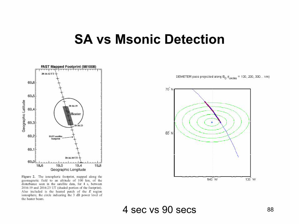
Detection time < 30

sec

SAW detection by DEMETER

63

1OO nT

Detection time>120

sec

No ground signals detectedMsonic wave detection by DEMETER

64

O+ Density

E-Field

PSD

Injected ULF power approximately 5-10 kW

65

Detection time > 100 sec

Msonic wave detection by DEMETER

66

S. Ganguly, W. Gordon and K. Papadopoulos PRL 1986

B

Msonic ground detection in Arecibo

67

UH heating

Bill Bristow UAL

B. Eliasson

K. Papadopoulos

Can we drive whistlers with F-region heating?

68


Propagation


SU - UCLA

RMFSU - UCLA


Amplification

VLF

ULF

VLF

VLF


SU

HAARP F-RegionUM

RMF - HEDUM

Natural DuctsBC

Artificial DuctsUM



LEPSU

LHWSUVLF

ULF

WIPPSU


VLF/ULF

EMICUM

Alfven WavesUM

69

≈25 pT

V ≈ 2x1020 m3

W=2/2μ ≈ 3x10-16J/m3

Total Energy ≈ 60 kJ

Tconf ≈100-200 sec

Power ≈300-600 Watts

reflection

R ≈.90-.95

L≈1.5

Pitch Angle Diffusion Coefficient for Protons at 1 Hz

.1-3. Hz

Need1-3 Hz to resonate with 30-100 MeV protons at L=1.5

 pT

days

1000

Lifetime vs. 

 = 1 pT

Scale D at = 1pTto get lifetime at larger 

Pick lifetime of 103 days and getpower needed

Energetic Proton Removal

70

60 KM

75 KM

120 KM

SAW A

M MP=IL

HED

For HMDP≈300 (M/1010 A-m2)2 Watts

Ground Based Antenna Choice

VED

• VED minimal injection

For VMDP≈(300/4) (M/1010 A-m 2)2 (δ/75 km)2 Watts

What about HED ?

VMD HMD

71

75 km

120 km

A≈1010 m2

BR

To inject 600 W we require ≈20-25 pT at 75 km, the bottom of the magnetized ionosphere.

RMF

Rotating Magnetic FieldA superconducting magnet rotating at ULF frequency has an image in phase and increases its power by a factor of 4. This innovative antenna design can give the required 600 W with a magnetic moment of 1010 A-m2

Innovative Antenna Design

72

• Rotating superconducting magnets are useful for frequencies of up to 10 Hz

• They are compact sources of large moments and can be used in arrays• Example design:

– Superconducting coil 5 m high x 5 m wide x 5 m long– 25 m2 area– 100 Amps DC current– 4 x 104 turns– M = 108 A-m2

• In LTS wire ($2/kA-m) this could be a few million dollars including Dewar, He refrigeration, and rotation (HTS wire is still $50/kA-m, Cu now ~$100/kA-m)

Superconducting RMF

73

What about Tesla Technology HED Revisited

l

leff

Figure 1: Antenna with return current

Δ

( / 2 ) ln[ / ( )](8 / ) ln[ / ( )]

L l l lR l l l

μ π δ δπ σ δ δ

= Δ += Δ +

2 2l δ<

σ mho/m .1 Hz 1 Hz 10 Hz

10-4 150 km 50 km 16 km

10-3 50 km 17 km 5 km

10-2 17 km 5 km 1.7 km

Resistive impedance dominates if

Traditional HED antennae operate in the reactive impedance region

74

Point HED Design

~Δ

Figure 2: Plan view of HED antenna

B ≈ .4(P /MW )1/ 2(l /10km)5 / 2(σ /10−3)1/ 2nT

PULF ≈≈ 5(P /MW )(l /10km)5(σ /10−3)kW

1 km

75

Supplementary Slides

76

Total energy = E= Volumex(b2/2μ)=20 (b/20 pΤ)2 kJPower required =P=E/T= 300 (b/20 pT)2 (60 sec/T) Watts

60 KM

75 KM

120 KM

SAW A

M MP=IL

(5/75)2 4

P≈300 (M/1010 A-m2) Watts

Energy – Power Requirements

77

Key Points• First observation of Magnetosonic waves in

the Pc1 range generated by modulated ionospheric heating using the HAARP heater

• Msonic waves generated by modulated collisionless F-region electron heating and are independent of the presence of elctrojet currents

• Detection by the Demeter satellite flying over HAARP indicate ULF power in excess of 5 kW

78

The Fundamentals• For Pc1 frequencies (.1-7 Hz) the ionosphere behaves as:

• A resonator for Shear Alfven (SA) waves, confined along the B lines with an almost vertical structure at high latitudes • A waveguide for Magnetosonic (MS) waves propagating isotropically and ducted horizontally over long distances

Bo Reflection due to gradη at one to two thousand km

Partial reflection at E-region

Standing SA wave

Ducted MS wave

79

SA Waves – Ionospheric Alfven Resonator (IAR)

Cash et al. 2006

k

E

B

b

SvgSA wave is guided along the B field

Reflections create standing wave structure

Notice

b·B=0

Natural SA waves

80

MS (Compressional) Waves Alfvenic Duct

k

Bb

Svg E

D=εΕ

VA

Alfvenic Duct

Notice b parallel to B

Isotropic Mode

AIC instability drives SA waves

SA waves mode converted at the boundary of duct and propagate laterally

as MS waves over large distances

Natural generation and ducting of MS waves

81

ULF Generation by Ejet Modulation

• Ejet modulation cannot drive b field parallel to ambient B. This type of modulation can create only SA waves. The waves cannot propagate laterally since they are evanescent in the Earth-Ionosphere Waveguide and do not couple to the Alfvenic Duct

• SA waves can be detected: (a) In the near zone below the heated spot and (b) By satellites over-flying the heated spot but confined to the magnetic flux tube that spans the heated spot.

D/E region heating + Electrojet

Evanescent in EI Waveguide

SA waves do not Excite Ionospheric Duct

82

ULF Signals at Juneau

• 28 April, 2007 UTC 05:01:00 – 05:05:45• Detected 1 Hz & 3 Hz peaks• Amplitudes at 1 Hz: 0.28 pT NS; 0.23 pT EW

2~ 1/b R EVANESCENT

83

IAR Excitation - HAARP

.25 Hz .5 Hz Natural lines

HAARP

84(Wright et al., J. Geophys. Res., 2003)

Satellite SA Detection - EISCAT

Few Watts

85

F-Region Msonic ULF GenerationCollisionless upper hybrid F-region modulated heating results in Δp exp(iωt) that drives a b exp(iωt) with having a component parallel to B (a msonic mode). The wave propagates isotropically but is reflected at the D/E region and is much weaker on the ground. It can be measured by satellites or at large lateral distances (skip zone)

MHD Simulation

Vr

b/Bºβ (Δp/p)ºβ

86

Example of F-Region Msonic Generation Detected by the Demeter satellite

1OO nT

O-mode at 4.4 MHz HAARP at 3.5 MW modulated at .1 Hz between 6:47:30 and 6:59:30 UT

No ejet

No D/E region Demeter pass

No ULF detection on the ground - .1 Hz detection at Demeter between 6:51:30 and 6:53:00

87

Example 08/24/07; 3.3 MHz O-mode; .2 Hz

Ez ~ 0.2 mV/m

PSDDemeter Trajectory

88

SA vs Msonic Detection

4 sec vs 90 secs

89

Proton Energy

<δB> at L = 1.5

Life Time

50 MeV 20 pT 820 days



Equilibrium Distribution Function g(α0) Vs. Pitch Angle α0

)/)(exp()( 220 δωωωω −−∝f

f0 = 6 Hz, δf = 0.7 f0

Life Time and Equilibrium Equatorial Particle Flux Distribution

90

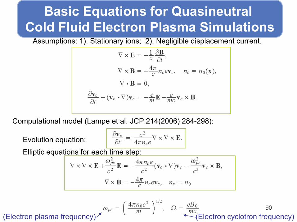
Assumptions: 1). Stationary ions; 2). Negligible displacement current.

Computational model (Lampe et al. JCP 214(2006) 284-298):

Evolution equation:

Elliptic equations for each time step:

(Electron plasma frequency) (Electron cyclotron frequency)

Basic Equations for Quasineutral Cold Fluid Electron Plasma Simulations

MURI REVIEW - University Of Marylandspp.astro.umd.edu/SpaceWebProj/RESEARCH PAGE PDFs n pics/1...

Documents

Transcript of MURI REVIEW - University Of Marylandspp.astro.umd.edu/SpaceWebProj/RESEARCH PAGE PDFs n pics/1...