MPRAMunich Personal RePEc Archive

When Do Large Buyers Pay Less?Experimental Evidence

Bradley J. Ruffle

Ben-Gurion University of the Negev

6. August 2009

Online at http://mpra.ub.uni-muenchen.de/16683/MPRA Paper No. 16683, posted 10. August 2009 14:12 UTC

When Do Large Buyers Pay Less?

Experimental Evidence

Bradley J. RuffleBen-Gurion University

August 2009

Abstract: The rise in mega-retailers has contributed to a growing literature on buyerpower and large-buyer discounts. According to Rotemberg and Saloner (1986) and Snyder(1998), large buyers’ ability to obtain price discounts depends on their relative (rather thanabsolute) size and the degree of competition between suppliers. I test experimentally com-parative statics implications of this theory concerning the number of sellers and the sizes ofthe buyers in the market. The results track the comparative statics predictions to a surpris-ing extent. Subtle changes in the distribution of buyer sizes or the number of suppliers cancreate or negate large-buyer discounts. The results highlight the previously unexplored roleof the demand structure in determining buyer-size discounts. Furthermore, the experimentsestablish the presence of small-buyer premia, not anticipated by the theory.

keywords: experimental economics, large-buyer discounts, buyer power, seller competition.

JEL classification nos. C92, D43.

Contact Information: Department of Economics, Ben-Gurion University, Beer Sheva, Israel,84105, e-mail: bradley@bgu.ac.il, tel.: +972-8-6472308, fax: +972-8-6472941.

Acknowledgements: I thank Shai Bernstein, Danny Cohen-Zada, Naomi Feldman, Hans Nor-mann, Jean Sauve, Christopher Snyder, Oscar Volij and seminar participants at Bar-Ilan University,Goethe University, Tel Aviv University and the APESA 2009 and IIOC 2009 meetings for usefulcomments. Ayala Waichman provided valuable research assistance. Tim Miller programmed theexperimental software.

1 Introduction

“’Now what is your best price?’ And if they told me it’s a dollar, I would say, ‘Fine, I’ll considerit, but I’m going to your competitor, and if he says 90 cents, he’s going to get my business. So,make sure a dollar is your best price.’” (Claude Harris, Wal-Mart’s first buyer, quoted fromWalton and Huey, 1993, p. 236)

The negotiating prowess of Wal-Mart buyers is renowned in buying/vendor circles . . . Vendorrelationships are important but the only guarantee of product continuity for vendors is tosharpen their pencils and to provide the best price, the first time it is requested. Failing to doso will lead to replacement in favor of a lower-cost provider. Competitive bids are encouragedand it is normal operating procedure for vendors to be pitted against one another . . . We didn’tcare what everyone else in the business world was paying for a product or service, we demandedthe lowest possible Wal-Mart price. (Bergahl, 2004, p. 30)

The academic literature and business press (see, e.g., Fishman 2003; Scherer and Ross

1990, pp. 528-529) often refer to two sources of buyer power: the buyer’s size and the intensity

of seller competition. In fact, as the above quotes from Wal-Mart’s first buyer and a former

Wal-Mart executive reveal, the world’s largest retailer extracts low prices from suppliers by

threatening to buy from the competition. The opportunity cost of not agreeing to Wal-Mart’s

price demands is the loss of a voluminous sale to a more conciliatory competitor.

In this paper, I examine experimentally how large a buyer needs to be in order to obtain a

lower price than its competitors. Size is measured as the number of units the buyer demands.

Is a buyer’s absolute size sufficient to determine whether a large buyer pays less? Or, is the

decisive measure a buyer’s size relative to other buyers in the market? What other aspects of

the demand structure are relevant in determining the existence and magnitude of large-buyer

discounts? What role does the degree of seller competition play in setting prices to buyers of

different sizes? To answer these questions, I test experimentally a number of parameterized

versions of a theoretical model that lay bear sellers’ considerations in deciding how much

to charge buyers of different sizes. In doing so, this is the first paper to bring to light the

importance of the demand structure in the prices that buyers pay.

The theoretical framework of this paper has its origins in Rotemberg and Saloner (1986)

(henceforth abbreviated as R-S). In their pioneering article, they demonstrate that periods

of high demand (booms) are most conducive to price wars since current demand is high

relative to future expected demand. To prevent price wars in booms, firms lower their

prices just enough so that deviation is no longer profitable. Snyder (1996, 1998) reinterprets

the macroeconomic shocks in R-S as buyers of different sizes arriving each period. Large

buyers entice sellers to underbid one another aggressively in an attempt to supply the large

quantities demanded. To prevent undercutting, sellers coordinate on lower prices when

confronted with a large buyer. Thus, similar to Wal-Mart, large buyers in Snyder (1996,

1998) obtain a discount through their ability to force sellers to compete in price with one

another. Notice that buyer size on its own is ineffective in this setup. Both in these models

and in my experiments, buyers of all sizes behave identically, purchasing all of their available

units of demand from the lowest-priced seller. As a result, buyers of all sizes would pay

the same price against a monopoly seller. It is the interaction between buyer size and seller

competition that yields, in some instances, buyer-size discounts.

In this paper, I parameterize the theoretical models of R-S and Snyder (1996, 1998) to

make more precise the influences of buyer size and seller competition. For instance, a merger

between two smaller buyers can negate the discount to the largest buyer in the distribution

by reducing the latter’s relative size. I test these and other predictions in controlled price-

setting experiments.

Across a number of experimental treatments, I vary the demand structure (i.e., number of

buyers in the market and size of each buyer) in a controlled manner that allows me to discern

the influence of the demand structure on sellers’ ability to collude as a function of buyer size.

In each period of these indefinitely repeated games, a buyer of randomly determined size

is drawn from a known distribution containing three of four buyer sizes. Symmetric sellers

each simultaneously offer a price at which to supply the buyer’s desired number of units,

with the lowest-priced seller fulfilling these units. All other higher-priced sellers earn zero.

Overall, I find that large-buyer discounts are rather robust: they are observed in the

experiments whenever predicted and even in some instances not predicted by the theory. Yet,

it is possible to negate the discount along lines suggested by the theory. The experiments

show, for instance, that through a reduction in the number of sellers, an increase in the

smaller-sized buyers in the market (through their merger, for instance) or shrinking the size

2

of the largest buyer (while maintaining the mean buyer size in the market) the large-buyer

discount can be eliminated. The experiments also uncover small-buyer premia, namely,

instances in which the smallest buyer in the market pays significantly more than all other

buyer sizes, despite predictions to the contrary.

In the next section, I review briefly the related literature. Section 3 summarizes R-S

and Snyder’s (1996, 1998) application of R-S to large-buyer discounts. In section 4, I detail

experiments designed to test the predictions of these models. Section 5 presents the results.

Section 6 concludes.

2 Related Literature

There is a growing literature that identifies a number of plausible sources of large-buyer

discounts.1 The starting point for the source of buyer-size discounts on which this paper

focuses is Rotemberg and Saloner (1986). In their setup, symmetric oligopolists face random

demand fluctuations in each period of an infinitely repeated game. When demand is high,

the benefit from undercutting the joint-profit-maximizing price is also high. To prevent

undercutting and possible price wars, firms settle on the highest sustainable price, namely,

the highest price at which the profit from unilaterally deviating from this price plus the

subsequent punishment profit falls just short of the present discounted collusive profit. The

implication is that collusive prices are lower in periods of high demand (booms) than in those

of low demand.

Snyder (1996, 1998) interprets the random demand shocks in R-S as a buyer of varying

size arriving each period. Large buyers tempt sellers to shade the monopoly price in order

to capture the entire demand for themselves. To prevent such out-of-equilibrium deviations,

sellers collude on lower prices against large buyers than against smaller ones, yielding the

large-buyer-discount result. Snyder (1996) endogenizes buyer size: buyers may carry over

unfilled units of demand to subsequent periods. By purchasing all of their backlogged demand

1 See Ruffle (2009) and Snyder (2008) for surveys.

3

at once, large buyers obtain low prices from sellers. To attenuate this off-equilibrium-path

threat, sellers may reduce their prices, even if the buyer purchases in every period. In

Snyder (1998) buyer size is exogenously determined with sellers facing a buyer of randomly

determined size each period.

Notice that the source of buyer-size discounts in these models in no way relies on large

buyers’ superior negotiation skills – a trait commonly attributed to large buyers. In fact,

buyers are essentially price-takers. It is the lucrative profit opportunity they represent that

induces sellers to compete vigorously with one another to supply their large demand. Put

differently, the interaction between buyer size and seller competition produces buyer-size

discounts in this framework.

While this is the first test of this source of buyer-size discounts, Normann et al. (2007)

test experimentally a theory of large-buyer discounts in a monopoly setting that depends on

the monopolist’s economies of scale. Consistent with the theory, their experiments reveal

large-buyer discounts only if the monopolist has increasing marginal costs.

There are a few experimental tests that relate to R-S. Abbink and Brandts (2009) design

experimental duopoly markets in which the total market demand follows a known evolution;

demand persistently shrinks in each of the 27 periods in one treatment and expands in

another. Thus, unlike R-S, demand shocks in both of their treatments are deterministic.2

Also unlike R-S, Abbink and Brandts observe higher prices in the shrinking market; namely,

sellers collude better when current demand is high relative to future demand.

List (2008) conducts field experiments in open air markets. With the goal of evaluating

the efficiency and collusive properties of these markets, he employs confederate buyers to

negotiate with sellers and an inside seller or “mole” who supplies information on existing

collusive agreements. Consistent with R-S, List finds that vendors in these markets cheat

more frequently on higher volume days.

Rojas (2009) examines the role of payoff information and monitoring in repeated two-

2 Their design is closer to Haltiwanger and Harrington (1991) and Kandori (1991) in which demand shocksare cyclical. These models’ predictions of lower prices when demand is declining are similarly violated.

4

person prisoners’ dilemma experiments with random shocks to payoffs. In one treatment

designed to capture the essential features of R-S, players observe the payoff shock prior to

choosing cooperate or defect and actions are ex post observable (i.e., perfect monitoring). In

line with R-S, defection is most likely when the high-payoff matrix is played.

In the context of large-buyer discounts, Ellison and Snyder (forthcoming) examine the

wholesale prices of pharmaceuticals with different substitution opportunities to buyers of

different sizes. Their empirical results validate the importance of seller competition for

volume discounts in addition to sheer buyer size. For instance, hospitals and HMOs –

buyers with the ability to substitute between off-brand drugs – pay substantially lower prices;

whereas, despite their size advantage, chain drugstores pay similar prices to independents,

even for off-patent drugs, because both are required to stock a range of substitute drugs in

case a customer walks in with a prescription for a particular drug. The authors conclude

that, “The finding of no size discounts for on-patent antibiotics is evidence against the

pure bargaining models which imply that large buyers can obtain price discounts even when

bargaining against a monopoly supplier.”

In this paper, I test experimentally the conditions under which price-setting sellers will-

ingly cede price discounts to large buyers. I make subtle changes in the demand and supply

structures predicted either to induce or negate a large-buyer discount. I then investigate

whether prices and in particular concessions to large buyers are responsive to these subtle

parameter changes. All experimental treatments involve at least two competing symmetric

sellers (as required by theory and supported by the results of Ellison and Snyder) facing a

buyer drawn randomly from a known distribution of differently sized buyers.

3 Model

Using the buyer-size framework, I summarize the models of R-S and Snyder (1998) in this

section. Consider the following infinitely repeated game with a time discount factor δ.

An industry consists of N symmetric suppliers, each producing a homogenous product at

5

constant marginal cost, which I normalize to 0. In each period t, the N suppliers each choose

a price, pit, and collectively face a single buyer of randomly determined size, st. Buyer size

st is drawn from the distribution F , which may either be a continuous interval, [s, s], or a

discrete range, {s, . . . , s}. The realization of F is observable to all players in the market.

Buyer i is assumed to purchase from the lowest-priced seller and thus a buyer’s strategy is

completely determined by its demand function D(pt, st), where pt = min{pit| i = 1, . . . , n}.

In the case that n ≤ N sellers set the same lowest price, each of these sellers supplies st/n

units. Assume that ∂D∂pt

≤ 0 (the law of demand holds) and also that ∂D∂st

≥ 0 (demand

increases with buyer size).

Like R-S, Snyder and others in this literature, I focus on the extremal equilibrium, namely,

the subgame-perfect equilibrium that maximizes the suppliers’ joint profit, and, also like the

previous literature, I assume that sellers employ grim trigger strategies, namely reversion to

the static Nash equilibrium in all periods following any seller’s deviation from the extremal

equilibrium price. The experimental results will allow us to evaluate this assumption. More

precisely, do sellers in fact respond to another’s deviation with indefinite punishment or do

they return to more cooperative pricing after some punishment of limited duration?

Let pm(st) represent the monopoly price for buyer size st and Πi(pm, st) seller i’s resultant

profit. By definition, this price maximizes the suppliers’ joint profits given by, Πm(st) =

[pm(st) − c] · D(pm(st), st). For any seller i, it is profitable to deviate in period t against a

buyer of size st if and only if,

N ·Πi(pm, st) +

δ

1− δ

∫ st

st

Πi(pNE, st)dF (st) ≥ Πi(p

m, st) +δ

1− δ

∫ st

st

Πi(pm, st)dF (st). (1)

The left-hand side of equation (1) represents the present discounted deviation profit com-

posed of the one-period profit from infinitesimally undercutting the monopoly price plus the

discounted punishment profit from setting the Nash equilibrium price for all future periods.

The right-hand side of the equation represents the present discounted profit from maintain-

ing the collusive price, pm, and is equal to a single seller’s one-period profit from monopoly

6

pricing plus the continuation profit from this price. Simplifying slightly,

(N − 1) · Πi(pm, st) +

δ

1− δ

∫ st

st

Πi(pNE, st)dF (st) ≥

δ

1− δ

∫ st

st

Πi(pm, st)dF (st). (2)

Define s∗ as the largest buyer for which the monopoly price is charged in equilibrium.

Snyder makes the following two assumptions to rule out two trivial cases in which the same

price is charged to buyers of all sizes:

N <1

1− δ(3)

Πm(s)

Es(Πm(s))>

δ

(1− δ)(N − 1)(4)

A violation of (3) yields marginal cost pricing as the only subgame-perfect equilibrium,

while if (4) is violated, monopoly pricing for all buyer sizes is the unique subgame-perfect

equilibrium. If both (3) and (4) hold, then Snyder establishes that s < s∗ < s, implying that

sellers deviate from the monopoly price for one or more buyer sizes greater than s∗.

The following proposition states this result formally.

Proposition 1. (Snyder 1998) In the extremal equilibrium, the price charged by all sup-

pliers, p(st), depends only on st and is independent of the pricing history. There exists

s < s∗ < s such that p∗(st) = pm(st) for st ≤ s∗ and such that p∗(st) declines with st for

st > s∗.

Proof: See R-S (1986, pp. 394-395) and Snyder (1998, p. 207).

R-S (p. 395) state two intuitive comparative statics results with respect to s∗: s∗ decreases

as either δ decreases or N increases. In the next section, I parameterize R-S and Snyder to

test the theory and the sensitivity of seller pricing to the number of sellers and the demand

structure. The goal is to gain an understanding of the circumstances under which large

buyers obtain price discounts.

7

4 Experimental Design and Procedures

4.1 Experimental Framework and Research Strategy

To test the theory and the range of parameters under which large-buyer discounts obtain,

I design a number of treatments. In each treatment, just like the theory, N symmetric

sellers face a buyer of size st in each period where the buyer’s randomly determined size

is drawn from a known distribution. After observing the buyer size, st, in round t, sellers

simultaneously choose prices. The buyers are computerized and employ the strategy assumed

in the model; namely, they purchase from the lowest-priced seller and, in case more than one

seller sets the lowest price, they divide their purchases equally among these sellers. After

buyers make their purchases, sellers observe their own round profits and the other sellers’

chosen prices. The round is over.

The theory applies to infinitely repeated games, the most credible laboratory implemen-

tation of which involves a repeated game with a known end-game probability, δ.3 Thus, in

any round t, the game continues to round t + 1 with probability δ, and the game ends with

probability 1− δ and, time permitting, a new game with a different cohort of sellers begins.

The impact of the buyer demand structure on seller pricing has not been tested. Thus,

rather than commit a priori to an entire experimental design only to find that all of the

treatments produce qualitatively similar results (e.g., no buyer-size discounts), I begin with

a treatment predicted and behaviorally likely to yield large-buyer discounts. I let the results

of this treatment inform my design of subsequent treatments according to the following

logic. If the initial treatment fails to produce large-buyer discounts, then I can, for instance,

increase the largest buyer’s size, holding all other buyer sizes constant. If this also fails,

I can continue to increase s or introduce an additional seller. On the other hand, if this

initial treatment yields the predicted large-buyer discount, I can shrink the largest buyer

sufficiently to negate the prediction of large-buyer discounts. If a discount to this buyer

3 See Roth and Murnighan (1978) for a classic laboratory study of infinitely repeated games and Feinbergand Husted (1993) for more recent infinitely repeated duopoly experiments.

8

nonetheless persists, I can explore additional directions in the demand and supply structures

expected to further weaken sellers’ incentives to deviate against the largest buyer.

4.2 Choice of Experimental Parameters

With the above experimental framework in hand, I still need to select parameters for the

specific treatments. Collusion in experiments with more than two sellers has been shown

to be unattainable (e.g., Isaac and Reynolds 2002), even in the generally less competitive

Cournot framework (Huck et al. 2004). The inability of three or more sellers to maintain

prices above the Nash equilibrium precludes buyer-size discounts or price variance more

generally. To avoid such a fate and in an effort to achieve some degree of cooperation such

that price variation as a function of buyer size is at least possible, I adopt a number of

measures. To begin, I limit the number of sellers to two (the minimum required by the

theory) or three in all treatments.

To further facilitate collusion and simplify sellers’ price choices, I reduce the price space

to three distinct prices, the monopoly price, pm, and two deviation prices, punder and ppunish,

where pm > punder > ppunish.4 The price punder can be thought of as the undercutting price,

while ppunish represents a punishment price. Consistent with these interpretations, I place

the following restriction on each of these prices.

punder · st >pm

N· st ∀st, N > 1 (5)

ppunish · st <pm

N· st ∀st, N > 1 (6)

Equation (5) indicates that the individual seller earns more in round t from undercutting

and supplying all of the buyer’s units than charging the collusive price and earning 1/N of

the total profit. Equation (6) requires a punishment price sufficiently low that deviation to

this price is not profitable, even in the short run.

4 In infinitely repeated-game experiments with imperfect monitoring, Feinberg and Snyder (2002) alsorestrict the price space to three, while Aoyagi and Frechette (forthcoming) and Rojas (2009) limit attentionto two quantity choices.

9

I assume that each buyer at time t has inelastic demand for st units of production,

st ∈ [s, s]. A buyer of size st values each of his units of demand at 10. This implies that

pm = 10. We can thus rewrite condition (1) for deviation against the largest buyer size, s,

from the monopoly price of 10 to the price below it, punder as,

punder · s +δ

1− δ·

s∑st=s

ppunish · st

M ·N>

10 s

N+

δ

1− δ

s∑st=s

10st

M ·N. (7)

The left-hand side of (7) is the round profit from deviating to punder plus the present dis-

counted punishment profit from all N sellers charging ppunish indefinitely. The right-hand

side of (7) is the seller’s share of the present discounted collusive profit from coordinating

on the collusive price of 10.

With these simplifications, I still need to choose the two deviation prices, the distribution

of buyer sizes and the continuation probability (equivalently, the discount factor), δ. Feinberg

and Husted’s (1993) duopoly experiments illustrate the importance of a high discount factor

to achieve collusion. However, if the discount factor is too high, the monopoly price will

be the equilibrium price for all buyer sizes. Likewise, if the undercutting price, punder, is

too low relative to the monopoly price, the latter may be the equilibrium price for all buyer

sizes. If, on the other hand, the undercutting price is too similar to the monopoly price,

then collusion may never be sustainable for any buyer size. To achieve the desired balance,

I choose the discount factor equal to 0.8, punder equal to 8 and ppunish equal to 2 and hold

constant these variables across the initial and all subsequent treatments.

A discount factor or continuation probability of 0.8 means that at the end of each round

with probability 0.8 the same game continues to the next round and with probability 0.2

the game ends and, time permitting, a new game begins with a different cohort of sellers.

Prior to conducting the experiments, I randomly determined the length of each of the six

repeated games, displayed in Table 1, and applied these realizations to all sessions and

treatments so that all seller cohorts regardless of session or treatment saw the identical

randomly determined sequence of game lengths.

An additional feature of my experimental design that allows for a controlled comparison

10

Repeated Game Lengths

Game Periods (T)

1 4

2 17

3 8

4 5

5 12

6 4

Table 1: The number of repetitions in each supergame. A perfect strangers design was employed betweengames.

of subjects’ behavior across seller cohorts and treatments is the use of a unique sequence

of randomly drawn buyer sizes. Practically speaking, I randomly drew one sequence of 70

buyer sizes (for the five practice rounds, the 15 rounds in Part 1 and 50 rounds in Part 2)

from a uniform distribution over four buyer sizes prior to beginning the experiments and

applied this sequence to all seller cohorts in all sessions and treatments facing a distribution

with four buyer sizes.5

4.3 Initial Treatment

The initial treatment I refer to as “mega-retailer” and display its details in the first column

of Table 2). In this treatment, three sellers face the above constants and a buyer-size distri-

bution F = {1, 2, 6, 14}. Deviation from the monopoly price is unprofitable against buyers

of sizes 1, 2 and 6; whereas, a one-time deviation to punder against the largest buyer of size 14

is profitable, yielding an excess present-discounted profit of 4 (as shown in the third-to-last

row in Table 2). Thus, the equilibrium prices (displayed in the last row of the table) are 10

for the three smallest buyers and 8 for the largest buyer of size 14.

We don’t anticipate prices to match the above equilibrium point predictions, in part be-

cause of the noted difficulty in achieving full collusion in laboratory experiments. Notwith-

5 Thus, for instance, in round 2 of game 1, rounds 1, 3, 9 and 16 of game 2, etc., sellers in all treatmentsface a buyer of size 6, the second largest buyer in all treatments.

11

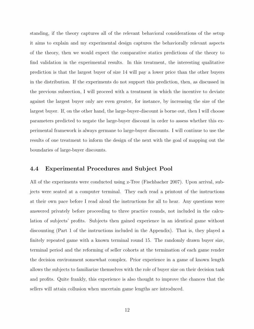
standing, if the theory captures all of the relevant behavioral considerations of the setup

it aims to explain and my experimental design captures the behaviorally relevant aspects

of the theory, then we would expect the comparative statics predictions of the theory to

find validation in the experimental results. In this treatment, the interesting qualitative

prediction is that the largest buyer of size 14 will pay a lower price than the other buyers

in the distribution. If the experiments do not support this prediction, then, as discussed in

the previous subsection, I will proceed with a treatment in which the incentive to deviate

against the largest buyer only are even greater, for instance, by increasing the size of the

largest buyer. If, on the other hand, the large-buyer-discount is borne out, then I will choose

parameters predicted to negate the large-buyer discount in order to assess whether this ex-

perimental framework is always germane to large-buyer discounts. I will continue to use the

results of one treatment to inform the design of the next with the goal of mapping out the

boundaries of large-buyer discounts.

4.4 Experimental Procedures and Subject Pool

All of the experiments were conducted using z-Tree (Fischbacher 2007). Upon arrival, sub-

jects were seated at a computer terminal. They each read a printout of the instructions

at their own pace before I read aloud the instructions for all to hear. Any questions were

answered privately before proceeding to three practice rounds, not included in the calcu-

lation of subjects’ profits. Subjects then gained experience in an identical game without

discounting (Part 1 of the instructions included in the Appendix). That is, they played a

finitely repeated game with a known terminal round 15. The randomly drawn buyer size,

terminal period and the reforming of seller cohorts at the termination of each game render

the decision environment somewhat complex. Prior experience in a game of known length

allows the subjects to familiarize themselves with the role of buyer size on their decision task

and profits. Quite frankly, this experience is also thought to improve the chances that the

sellers will attain collusion when uncertain game lengths are introduced.

12

Game Constants, Parameters, Profits and Equilibrium Prices

Treatment

Constants mega-retailer large buyer 2 sellers buyer merger same mean

pm, punder, ppunish 10, 8, 2 10, 8, 2 10, 8, 2 10, 8, 2 10, 8, 2

δ 0.8 0.8 0.8 0.8 0.8

Parameters

Sellers (N) 3 3 2 3 3

Buyers (M) 4 4 4 3 4

Buyer Size 1 (LB) 14 10 10 10 8

Buyer Size 2 6 6 6 6 6

Buyer Size 3 2 2 2 3 3

Buyer Size 4 (SB) 1 1 1 — 2

net PDV deviation against LB 4 −4 −46 −20.89 −13.33

Deviate against LB? Yes No No No No

Eq’m Prices by Buyer Size 8, 10, 10, 10 10, 10, 10, 10 10, 10, 10, 10 10, 10, 10 10, 10, 10, 10

Table 2: For all five treatments, the three available prices and discount factor are held constant. Thefive treatments differ by the number of sellers (N) and buyers (M) in the market and the distribution ofbuyer sizes. The net discounted profit from deviation against the largest buyer (LB) in the distribution(from equation (7)) and, as a result, whether sellers have an incentive to deviate from pm against LB andequilibrium prices by treatment and buyer size (in descending order) are displayed in the last three rows.

At the completion of Part 1, subjects proceeded to Part 2 (see the Appendix for the in-

structions), the core of the experiment in which the terminal round in each game is randomly

determined. At the end of the practice rounds, the 15 rounds from Part 1 and each repeated

game in Part 2, seller groups are randomly reformed conditional on not having previously

been in the same group as any of the other sellers in their present group. Namely, a perfect

strangers design is employed between games to minimize the dependence between games.

Because of the economic nature of this experiment and the types of reasoning and com-

putations required of subjects, I restricted recruitment to economics and business majors.

In total, 172 subjects participated in one of five treatments. Including the instruction phase,

the three practice rounds, the 15 known rounds of Part 1, the six games with randomly

determined terminal rounds in Part 2 and the post-experiment questionnaire, each session

13

lasted about one hour and 45 minutes. Average subject earnings were 71.6 NIS (s.d. = 15.1

NIS) or about $19 USD, well above the student wage of 19 NIS an hour.

5 Results

To examine buyer-size discounts I rely on two measures, sellers’ offers and prices paid by

buyers. In almost all cases, the qualitative results are identical regardless of which measured

is used. In some sense the price paid is more meaningful since prices, not offers, ultimately

determine whether a buyer receives a discount. Also, outside the laboratory, prices, not

offers, are observable, if at all. On the other hand, offers provide a fuller dataset with an

observation for each seller in every round.

1. mega-retailer

Thirty subjects participated in this initial treatment. The first four rows of Table 3 and

the top graph in Figure 2 display the mean offers and prices paid by buyer size. The first

noteworthy observation is that the mean offers and prices are well above the punishment price

of 2 for all four buyer sizes, indicating both that the measures taken to achieve collusion

(e.g., only three available prices, a relatively high continuation probability) succeeded to

some degree and that punishment strategies are not played indefinitely. At the same time,

mean offers and prices well below the collusive price of 10 raise the possibility that sellers

charge more to the smallest buyer in the distribution than to mid-sized buyers. For perfectly

inelastic demand curves, the theory does not admit such a possibility, instead predicting the

same monopoly price for all buyers st < s∗.6 I evaluate small-buyer premia below.

Mean offers decrease monotonically in buyer size with the sharpest drop from buyer size 6

(6.91) to the largest buyer 14 (5.87). Mean prices reveal an even bigger large-buyer discount.

The mean price is around 7 for the two smallest buyer sizes of 1 and 2, falls to 6.15 for buyer

size 6 and swoons by more than a full point to 4.85 for the largest buyer of size 14. In

6 Snyder (1998, pp. 207-208) provides an example with individual downward-sloping demand curves, eachwith a vertical intercept of st, in which the extremal equilibrium price (equal to the monopoly price) actuallyincreases with buyer size up to s∗.

14

percentage terms, the two smallest buyers each pays about 45% more than buyer size 14,

while buyer size 6’s price premium is 27%.

Tables 4 – 8 report ordered probit regressions for each of the five treatments. The

dependent variable is seller i’s round t offer (the first three regressions in each table) or the

lowest offer in each market in round t (namely, the price paid) (the fourth regression in each

table) with each of the three prices, 2, 8 and 10, as the possible realizations of the dependent

measure. The standard errors reported are robust to heteroskedasticity and are corrected

for possible non-independence of observations across rounds of play for the same seller by

clustering on each seller’s observations in the offer regressions7 and on the seller-cohort-game

cell in the price regressions. The basic ordered probit results in (1) of Table 4 show that

sellers offer significantly higher prices to all buyer sizes compared to buyer size 14.

The large-buyer discount is robust to the inclusion of controls for the overall round (round)

and the sequence of the repeated game (game) in (2). The coefficient on round is negative and

highly significant, while the coefficient on game is positive and highly significant. Together

these findings suggest that collusion erodes over time, but is restored in some measure at

the beginning of each new game.8 The interaction of round with each of the four buyer-

size indicators in (3) shows that offers decline significantly over time for the three largest

buyers; however, the coefficient of −.009 on round∗BS1 is not significantly different from

zero (p = .275). Sellers appear better able to sustain collusion over time on the smallest

buyer.

In fact, Wald tests on the coefficients of BS1, BS2 and BS6 in (2) indicate that, controlling

for the above time trends, offers to buyer size 1 are higher than those to sizes 2 and 6

7 I also tried clustering more finely on the seller-game cell. All results are identical.8 I observe this same pattern of declining offers over rounds, but offer increases with each new game

in all subsequent treatments as well. This restart effect is commonly found in finitely repeated versionsof another cooperation game, the public goods game, especially when the same cohort of subjects remainstogether for subsequent repeated games (see, e.g., Andreoni and Croson 2008). Engle-Warnick and Slonim(2006) demonstrate that trusting behavior displays a restart effect in indefinitely repeated trust games. Theyalso show that trust and trustworthiness are positively associated with the realized length of the previousindefinitely repeated game (their “Lag length” variable in Table 2). Similarly, Lag length is highly significantand positive in the offer, but not the price, regressions of this and all subsequent treatments. I elect not toreport it because this effect is far removed from the topic of this paper and the significance of the buyer sizeindicators remain unaffected by its inclusion.

15

(z = 2.51, p = .01 and z = 5.28 and p < .001, respectively). Similarly, offers to size

2 are higher than those to size 6 (z = 3.73, p < .001). In words, sellers graduate their

offers to account for buyer size, leading to both a significant smallest-buyer premium and a

largest-buyer discount.

I use my main offer regression of interest (2) to compute the mean predicted probabilities

of choosing each of the three available prices by buyer size, with the round and game variables

evaluated at their mean values. The right-hand columns of Table 3 display these predicted

probabilities. The probability assigned to any of the three prices differs by no more than

0.06 between the two smallest buyer sizes. For instance, with probability 0.79 sellers choose

price 8 for both these buyer sizes with the remaining 0.21 split not too unequally between

prices 2 and 10. However, the entries reveal a modest shift in the probability distribution

toward a price of 2 for buyer size 6 (.207) and a larger shift for buyer size 14 with probability

.365 placed on price 2 and a mere .013 on price 10.

I repeat the above regression analysis with the price in round t as the dependent variable.9

The estimates in (4) reveal that the highly significant quantity discount for buyer size 14 with

respect to all smaller buyers holds for prices paid as well. The smallest-buyer premium is less

robust: Wald tests indicate that the two smallest buyers pay similar prices to one another

(z = 1.01, p = .31), whereas both pay significantly more than buyer size 6 (z = 2.56, p = .01

and z = 2.14, p = .03 for BS1 and BS2, respectively).

Having observed in this treatment a significant large-buyer discount anticipated by the

theory, I next design a treatment predicted to negate the discount to determine whether

sellers in the experiments behave accordingly.

2. large buyer

This treatment makes one subtle change to the mega-retailer treatment: the largest buyer

is reduced in size from 14 to 10, resulting in the buyer-size distribution F = {1, 2, 6, 10}. As

9 To save space, I report only the regression corresponding to (2). The results of the regressions analogousto (1) and (3) are qualitatively similar to the offer regressions in this and all subsequent treatments. Anydifferences will be noted as they arise.

16

Table 2 shows, this single change renders unprofitable a deviation from the monopoly price

against the largest buyer. The net discounted profit from deviation against the largest buyer

of size 10 is −4, compared to 4 against size 14 in mega-retailer.

Thirty subjects participated in this treatment. Table 3 and the top-left panel of Figure

2 display the mean offers and prices paid by buyer size in this large buyer treatment.

Once again, both the mean offers and prices decline monotonically with buyer size. Mean

offers are 7.52 to the smallest buyer, decreasing to 6.74, 6.41 and 5.68 to buyer sizes 2, 6

and 10, respectively. Like the mega-retailer treatment, the large-buyer discount is even more

pronounced if, instead of offers, we consider the prices paid. The large buyer pays 4.17,

25.5% less than buyer size 6, with this discount ballooning to 57% compared to the smallest

buyer.

The regressions in Table 5 confirm the significance of the large-buyer discount with respect

to all smaller buyers in all specifications. Based on regression (6), the mean predicted offer

probabilities in Table 3 reveal that as buyer size increases the probabilities with which sellers

choose price offers of 10 and 8 progressively fall, while price offers of 2 steadily increase. Wald

tests confirm the significance of the smallest buyer premium (BS1) compared to the second

smallest buyer (BS2) in both offers (z = 4.19, p < .001) and in prices (z = 2.57, p = .01).

On the other hand, the two intermediate-sized buyers (BS2 and BS6) pay similar prices

(z = 1.39, p = .16).

In summary, the smallest buyer (of size 1) pays a significant premium with respect to

all other buyers, a reasonable result not predicted by the theory. The theory does correctly

predict that the mid-sized buyers in the distribution (of sizes 2 and 6) pay similar prices

to one another. Finally, the largest buyer obtains a substantial price discount compared to

the prices offered to and paid by all smaller buyer sizes. Because this large-buyer discount

was not anticipated by the theory, one may begin to wonder whether large-buyer discounts

are ubiquitous, as the public commonly perceives. Perhaps subjects are so accustomed to

large-buyer discounts that they instinctively respond by offering a lower price whenever the

large buyer appears.

17

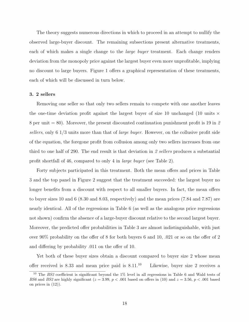
The theory suggests numerous directions in which to proceed in an attempt to nullify the

observed large-buyer discount. The remaining subsections present alternative treatments,

each of which makes a single change to the large buyer treatment. Each change renders

deviation from the monopoly price against the largest buyer even more unprofitable, implying

no discount to large buyers. Figure 1 offers a graphical representation of these treatments,

each of which will be discussed in turn below.

3. 2 sellers

Removing one seller so that only two sellers remain to compete with one another leaves

the one-time deviation profit against the largest buyer of size 10 unchanged (10 units ×

8 per unit = 80). Moreover, the present discounted continuation punishment profit is 19 in 2

sellers, only 6 1/3 units more than that of large buyer. However, on the collusive profit side

of the equation, the foregone profit from collusion among only two sellers increases from one

third to one half of 290. The end result is that deviation in 2 sellers produces a substantial

profit shortfall of 46, compared to only 4 in large buyer (see Table 2).

Forty subjects participated in this treatment. Both the mean offers and prices in Table

3 and the top panel in Figure 2 suggest that the treatment succeeded: the largest buyer no

longer benefits from a discount with respect to all smaller buyers. In fact, the mean offers

to buyer sizes 10 and 6 (8.30 and 8.03, respectively) and the mean prices (7.84 and 7.87) are

nearly identical. All of the regressions in Table 6 (as well as the analogous price regressions

not shown) confirm the absence of a large-buyer discount relative to the second largest buyer.

Moreover, the predicted offer probabilities in Table 3 are almost indistinguishable, with just

over 90% probability on the offer of 8 for both buyers 6 and 10, .021 or so on the offer of 2

and differing by probability .011 on the offer of 10.

Yet both of these buyer sizes obtain a discount compared to buyer size 2 whose mean

offer received is 8.33 and mean price paid is 8.11.10 Likewise, buyer size 2 receives a

10 The BS2 coefficient is significant beyond the 1% level in all regressions in Table 6 and Wald tests ofBS6 and BS2 are highly significant (z = 3.99, p < .001 based on offers in (10) and z = 3.56, p < .001 basedon prices in (12)).

18

discount in both offers and prices compared to buyer size 1 whose mean offer (price) is 8.65

(8.28) (z = 5.28, p < .001 and z = 2.70, p = .01 based on Wald tests on (10) and (12),

respectively). In other words, the prices to the smallest buyer are significantly higher than

to all other buyers again in this treatment.

In addition, offers and prices for all four buyer sizes in 2 sellers appear to be substantially

higher than their counterparts in large buyer. Huck et al.’s (2004) meta-analysis of Cournot

experiments (with symmetric buyers) along with their own results also find two sellers better

able to collude than three.

The next two treatments both involve more subtle changes involving the buyer demand

structure. In the next buyer merger treatment, I increase the mean buyer size by merging the

two smallest buyers in the distribution, while holding constant the size of the largest buyer.

In the same mean treatment, I shrink the largest buyer, while holding constant the mean

buyer size. As the deviation equation (1) makes clear, both of these changes are predicted

to strongly discourage deviation against the largest buyer.

4. buyer merger

In this fourth treatment, I merge the two smallest buyers of sizes 1 and 2 into a single

buyer of size 3 such that F = {3, 6, 10}. This subtle alteration in the demand structure

effectively increases the mean buyer size from 4.75 to 6.33. This 33% increase in the mean

buyer size stems from two sources: i) the merged buyer is, by definition, larger than either

of its component buyers; ii) the reduction in the number of buyers from four to three, which

engenders an increased probability that sellers will face a buyer of size 10 or 6 in any given

round. The end result is that deviation against the largest buyer of size 10 is now considerably

more unprofitable (yielding a profit shortfall of 21) than in the large buyer treatment.

Thirty-three subjects participated in this treatment. The mean offers and prices to all

three buyer sizes are displayed in Table 3 and the bottom-left panel of Figure 2. To buyer

sizes 6 and 10, mean offers (7.09 and 6.93, respectively) and mean prices (6.49 and 6.25,

respectively) differ by no more than 3% from one another. The ordered probits in Table 7

19

reveal that offers to buyer size 6 are marginally significantly higher than offers to buyer size

10 in the absence of additional controls (13). Moving across columns, even this marginal

large-buyer discount disappears when time controls are included: the coefficients on BS6 in

(14) and (15) are not significantly different from zero (p = .16 and p = .81, respectively).

The predicted offer probabilities based on (14) support this finding with similar probabilities

on price offers across all three buyer sizes. In fact, the probabilities of any given offer never

differ by more than .035 between buyer sizes 6 and 10.

For prices, the regression results offer no trace of a significant discount to buyer size 10

compared to size 6: BS6 is not significantly different from 0 (p = .22) in (16), which includes

controls for round and game, nor in a price regression corresponding to (13) without these

controls (p = .38) (not reported), nor in a price regression corresponding to (15) (p = .30)

(also not reported). In summary, once again as predicted the largest buyer does not receive

an unambiguous discount compared to the second largest buyer.

Table 7 also reveals a substantial small-buyer premium. The coefficients on BS3 are

positive and highly significant in all of the regressions. Moreover, offers and prices to buyer

size 3 are significantly greater than those to size 6 in all regressions (p < .01 in all Wald tests

of the coefficients on BS6 and BS3 in (13) – (16)).

How do the prices paid by the merged buyer in this treatment compare to those of the

pre-merger buyers of sizes 1 and 2 in the otherwise identical large buyer treatment? The

model predicts the same monopoly price of 10 for all three buyer sizes. Notwithstanding,

we’ve already anticipated and observed offers and prices well below this level. This allows

for the behaviorally sensible outcome that the merged buyer pays less than the component

pre-merger buyers.11 On the contrary, Table 2 reveals that mean offers and prices to the

merged buyer (7.40 and 6.74, respectively) are significantly higher than those to size 2 in

large buyer.12 In fact, mean offers and prices to buyer size 3 resemble more closely and are

11 Snyder (1996) shows that a merger benefits both the merged buyer and all other buyers in the form oflower prices in a setup in which multiple, variously sized buyers are simultaneously present in the marketand each buyer is able to carry over unfulfilled units of demand to the next period.

12 P-values are less than .01 for both non-parametric Wilcoxon-Mann-Whitney tests where, to minimizethe dependence between observations, I take the average of all offers or prices in a seller cohort and a game

20

statistically indistinguishable from those of size 1 in large buyer.13

One plausible explanation for this paradoxical finding is that prices in buyer merger, as

in 2 sellers, are sharply higher than those in large buyer. Here, fewer deviations and the

less frequent use of punishment prices attest to sellers’ ability to better collude against the

largest buyer in buyer merger; whereas, when collusion breaks down on buyer size 10 in large

buyer, sellers mete out punishment not only on this buyer, but on smaller buyers as well.

5. same mean

In this final treatment, I return to a buyer-size distribution with four distinct buyer

sizes and a mean size of 4.75. Here, I shrink the size of the largest buyer from 10 to 8,

while compensating with a two-unit increase in the smallest buyer’s size from 1 to 3. In

brief, F = {2, 3, 6, 8}. All other experimental parameters (e.g., number of sellers, discount

factor, realized game lengths) are the same as in large buyer. As equation (1) reveals, holding

constant the mean buyer size while shrinking the largest buyer necessarily reduces the appeal

of deviation. Table 2 shows that the net shortfall from deviating against the largest buyer

drops from −4 in large buyer to −13.33 in same mean.

Thirty-nine subjects participated in this treatment. The mean offers and prices appear

in the bottom four rows of Table 3 and the bottom-right panel of Figure 2. To the largest

and second-largest buyers of sizes 8 and 6, mean offers (7.19 and 7.32, respectively) and

mean prices (6.69 and 6.44) once again appear similar to one another, as the theory predicts.

Mean offers and especially prices rise more substantially for buyer size 3 (7.76 and 7.38) and

still further for buyer size 2 (8.17 and 7.63).

Except for the basic offer regression in (17) in which round and game controls are absent,

offers and prices to buyer sizes 6 and 8 are not significantly different from one another

in any of the other regressions (including the analogous price regressions not reported). All

regressions do, however, reveal a highly significant discount to the largest buyer in comparison

to the smaller buyers of sizes 2 and 3. Similarly, offers and prices to buyer size 6 are

as the unit of observation.13 All of the results are unchanged if, less conservatively, I treat each offer or price as the unit of observation.

21

appreciably lower than those to sizes 2 and 3 (p < .02 or less in all four pairwise Wald tests

based on (18) and (20)).

The predicted offer probabilities based on the ordered probit estimates in (18) reinforce

the lack of a largest-buyer discount with respect to the second-largest buyer. For these two

buyers, the offer probabilities on any of the three available prices differ merely by between 1.3

and 1.7 percentage points. For both buyer sizes, sellers choose the price 2 with probability

.13 or so, price 8 with about probability .8 or so and price 10 with about probability .05.

By comparison, for the smallest buyer, sellers resort to the punishment price only 3% of the

time, while they set the collusive price about one-fifth of the time. These comparisons with

the smallest buyer size attest to the previously noted small-buyer premium with respect to

the two largest buyers. Further comparisons of the offer probabilities between buyer sizes

2 and 3 suggest that the smallest buyer pays more than buyer size 3 as well. Wald tests

confirm this (p < .001 in (18) and p = .03 in (20)).

6 Conclusions

In this paper, I design a number of experimental treatments to evaluate a plausible and

often-cited explanation for large-buyer discounts in the retail sector. According to this

explanation and the accompanying theory, buyers pay less if they are sufficiently large relative

to other buyers in the industry and there exists sufficient competition between sellers for their

business. My experiments test this theory by varying the distribution of buyer sizes in an

industry, the relative size of the largest buyer and the number of competing sellers in ways

that either create or negate seller incentives to charge less to the largest buyer.

The results mostly support the comparative statics predictions: seller pricing responds to

subtle changes in the demand structure and number of sellers along the lines of the theory.

Large buyers obtain discounts where predicted and even if the incentive not to charge less to

large buyers is sufficiently weak. To nullify the discount, the experiments elucidate several

possibilities such as fewer sellers, the merger of smaller buyers and shrinking the largest buyer

22

while maintaining the average buyer size in the industry. One robust finding not anticipated

by the theory is the presence of price premium to the smallest buyer in all five treatments.

There are two senses in which the results underestimate the presence and magnitude of

large-buyer discounts and small-buyer premia. First, the observed negation of the large-

buyer discount centers on a comparison between the largest and the second-largest buyers.

Compared to other smaller buyers in the market, the largest buyer always pays significantly

less in all treatments studied. Second, these experiments focus on a single explanation,

controlling for other explanations possibly present outside the laboratory. To the extent

that large buyers also benefit from a credible threat of backward integration, supply-side

scale economies, experience and superior negotiating skills, the price discrimination found

here will be amplified.

References

Abbink, Klaus and Brandts, Jordi (2009) “Collusion in Growing and Shrinking Markets:Empirical Evidence from Experimental Duopolies,” in Experiments and Antitrust Pol-icy, J. Hinloopen and H.-T. Normann (eds.), Cambridge University Press, Cambridge.

Andreoni, James and Rachel Croson (2008) “Partners versus Strangers: The Effect of Ran-dom Rematching in Public Goods Experiments, in Handbook of Experimental Eco-nomics Results, C. R. Plott and V. L. Smith (eds.), North Holland.

Aoyagi, Masaki and Guillaume R. Frechette (forthcoming) “Collusion as Public MonitoringBecomes Noisy: Experimental Evidence,” Journal of Economic Theory.

Bergahl, Michael (2004) “What I Learned from Sam Walton: How to Compete in a Wal-Mart World,” John Siley & Sons: Hoboken, NJ.

Ellison, Sara Fisher and Christopher M. Snyder (forthcoming) “Countervailing Power inWholesale Pharmaceuticals,” Journal of Industrial Economics.

Engle-Warnick, James and Robert L. Slonim (2006) “Learning to Trust in IndefinitelyRepeated Games,” Games and Economic Behavior, 54, 95-114.

Feinberg, Robert M. and Thomas A. Husted (1993) “An experimental test of discount-rateeffects on collusive behavior in duopoly markets,” Journal of Industrial Economics,41:2, 153-160.

23

Feinberg, Robert and Christopher Snyder (2002) “Collusion with secret price cuts: an ex-perimental investigation,” Economics Bulletin, 3:6, 1-11.

Fischbacher, Urs (2007) “z-Tree: Zurich Toolbox for Ready-made Economic Experiments,”Experimental Economics, 10:2, 171-178.

Fishman, Charles (2003) “The Wal-Mart You Don’t Know,” Fast Company, December: 77,68.

Haltiwanger, John and Joseph E. Harrington Jr. (1991) “The Impact of Cyclical DemandMovements on Collusive Behavior,” RAND Journal of Economics, 22:1, 89-106.

Huck, Steffen, Hans-Theo Normann and Jorg Oechssler (2004) “Two are Few and Four areMany: On Number Effects in Cournot Oligopoly,” Journal of Economic Behavior andOrganization, 53, 435-446.

Isaac, R. Mark and Stanley S. Reynolds (2002) “Two or Four Firms: Does It Matter,” inResearch in Experimental Economics, (C. Holt and R. M. Isaac, eds.), vol. 9, JAI-Elsevier: Amsterdam.

Kandori, Michihiro (1991) “Correlated Demand Shocks and Price Wars during Booms,”Review of Economic Studies, 58:1, 171-180.

List, John A. (2008) “The Economics of Open Air Markets,” unpublished manuscript.

Normann, Hans-Theo, Bradley J. Ruffle and Christopher M. Snyder (2007) “Do Buyer-SizeDiscounts Depend on the Curvature of the Surplus Function? Experimental Tests ofBargaining Models,” RAND Journal of Economics, 38:3, 747-767.

Rojas, Christian (2009) “The Role of Information and Monitoring on Collusion,” unpub-lished manuscript.

Rotemberg, Julio and Garth Saloner (1986) “A supergame-theoretic model of businesscycles and price wars during booms,” American Economic Review, 76, 390-407.

Roth, Alvin K. and J. Keith Murnighan (1978) “Equilibrium Behavior and Repeated Playof the Prisoner’s Dilemma,” Journal of Mathematical Psychology, 17, 189-198.

Ruffle, Bradley J. (2009) “Buyer Countervailing Power: A Survey of the Theory and Exper-imental Evidence,” in Experiments and Antitrust Policy, J. Hinloopen and H.-T. Nor-mann (eds.), Cambridge University Press: Cambridge.

Scherer, Frederic M. and David Ross (1990) Industrial Market Structure and EconomicPerformance, 3rd ed., Houghton Mifflin: Boston, MA.

Snyder, Christopher M. (1996) “A Dynamic Theory of Countervailing Power,” RAND Jour-nal of Economics, 27, 747-769.

Snyder, Christopher M. (1998) “Why Do Large Buyers Pay Lower Prices? Intense SupplierCompetition,” Economics Letters, 58, 205-209.

24

Snyder, Christopher M. (2008) “Countervailing Power,” in The New Palgrave Dictionaryof Economics 2nd edition, Steven N. Durlauf and Lawrence E. Blume (eds.), PalgraveMacmillan.

Walton, Sam and John Huey (1993) Sam Walton: Made in America, Bantam Books: NewYork.

Appendix

(Instructions for mega-retailer treatment)

Participant Instructions - Part 1

IntroductionThis is an experiment in the economics of market decision-making. Funds for this experiment

have been provided by various research foundations. Take the time to read carefully the instructions.A good understanding of the instructions and well thought out decisions during the experiment canearn you a considerable amount of money. All earnings from the experiment will be paid to you incash at the end of the experiment.

In this experiment, we are going to create numerous markets. All participants in these marketsact as sellers. In each market, there will be 3 sellers of a fictitious commodity. You will participateas a seller along with 2 other sellers in your market. There are two parts to this experiment. Inthe first part of the experiment, each market will be repeated with the same group of sellers for 15periods.

Random Buyer Size and Seller PricingIn each period, you and the other 2 sellers will face one computerized buyer of a randomly

determined size. The buyer’s size is drawn from a uniform distribution from the values 14, 6, 2 and1. So, there is an equal chance (1/4) that the buyer will be of size 14, of size 6, of size 2 and of size1. The buyer’s size indicates the number of units the buyer is interested in purchasing. Thus, forexample, a buyer of size 14 wishes to purchase 14 units, while a buyer of size 1 seeks to purchasea single unit.

As a seller, you and the other 2 sellers will simultaneously choose a price each period. Eachseller privately selects one of the following 3 prices: 10, 8, 2. If you all choose the same price,then you share equally the number of units demanded by the buyer. Your profit in this case isdetermined by the number (or fraction of the number) of units supplied, multiplied by the price.If you choose different prices, then the seller (or sellers) who selected the lowest price supplies thenumber of units demanded by the buyer. The profit of the lowest-priced seller (or sellers) is againgiven by the number (or fraction of the number) of units supplied multiplied by the chosen price.Note that sellers do not incur any cost for the units they supply: their costs of production are zero.

ExampleTo illustrate this game, consider the following example with a buyer of size 6. This means the

buyer seeks to purchase 6 units and will pay whatever price you charge. If you and the other 2sellers all choose the same price, then you each supply 6/3 = 2 units at the price selected. Thus,you each earn 2 units times the price selected. If all of the prices are not the same, then the sellerwith the lowest price supplies all 6 units at the price he selected. The other higher-priced sellers

25

each earn 0. If it is the case that more than one seller chose this same lowest price, then thesesellers split the 6 units equally between them at the chosen price.

Each PeriodYou will observe the outcome of your price decision at the end of each period. That is to say,

you will observe the number of units you supplied to the buyer, your profit for the period and theother 2 sellers’ chosen prices.

In each of the 15 periods, you and the same 2 other sellers will face the identical set of 3 pricesfrom which to choose. The only change between periods is the randomly determined size of thebuyer you face together: in each period, the number of units the computerized buyer seeks topurchase is chosen with equal probability from the sizes 14, 6, 2, 1.

PaymentsAt the completion of the second part of experiment, you will be paid your cumulative earnings

from all 15 rounds. Your earnings will be paid in cash at a rate of 1 shekel for every 15 units ofprofit you accumulate.

Before Beginning the ExperimentBefore beginning the experiment, the experimenter will read aloud the instructions. Next,

you will also be asked to answer a number of questions on the computer to confirm that youhave understood the rules of the experiment. Finally, you will participate in 5 practice roundsto allow you to familiarize yourself with the software and improve further your understanding ofthe experiment. The profit from these practice rounds will not count toward your cash paymentfrom the actual experiment. Otherwise, the rules from the 5 rounds are identical to those of theexperiment. At the end of the 5 practice rounds, you will be randomly rematched with 2 differentsellers with whom you will participate in the 15 rounds of play.

If at any stage you have any questions about the instructions, please raise your hand and amonitor will come to assist you.

Participant Instructions - Part 2This part of the experiment is identical to Part 1, except that instead of playing one game

consisting of 15 rounds, you will play a number of games one after another, each game of randomlydetermined length.

To repeat the basic rules, once again you will be matched with 2 other sellers. You will face abuyer of randomly determined size in each round. The buyer’s size (meaning the number of unitsthe buyer wishes to purchase) is either 14, 6, 2 or 1. Each of these four buyer sizes occurs with anequal probability of 1/4. At the beginning of each round, you will be shown the buyer’s size andneed to choose a price 10, 8 or 2. Your profit in a round is determined by your price, its relationto the other 2 sellers’ prices and the size of the buyer. The seller with the lowest price supplies allof the buyer’s demand at the price selected. If more than one seller chooses the same price, thenthey share equally the demand at the price chosen. Any seller that chooses a higher price earns 0for that round.

Number of PeriodsIn the first game, you will again be randomly matched with 2 sellers. The number of periods in

which you will participate with this same pair of sellers will be randomly determined. At the endof each period, a computer-generated random number between 1 and 100 will determine whetheryou proceed to the next period with the same set of sellers. If the random number is less than orequal to 80, you and the other 2 sellers will play another period together. You will continue to play

26

together for additional periods as long as the randomly generated number at the end of the periodis less than or equal to 80.

If, at the end of a given period, the random number is greater than 80, you will cease toparticipate in this market and, time permitting, begin to participate in an identical market withthe sole change being the other 2 seller participants. The rules in this new market are the same asthe previous one (i.e., same number of sellers, randomly determined buyer size each period, sameset of prices to choose from); the only difference is that you will be matched in this new market with2 sellers randomly selected from the group of participants with whom you have not participatedin a previous market. You will continue to interact with this same new cohort of 2 sellers for asmany periods as a random number less than or equal to 80 is drawn. If a number greater than 80is drawn at the end of a period, then, time permitting, you will again be rematched to play in athird market with 2 new sellers.

In short, in any given round, there is a 0.8 probability that the game will continue to the nextround and a 0.2 probability that the game will end at the completion of the current round. If, infact, the game comes to an end, then you will be rematched with 2 sellers in the next game, timepermitting, and continue to play in a market with them until that game ends. You will continueto play in a game until the random draw between 1 and 100 determines that the game ends. Youwill play as many games as time permits.

PaymentsAt the completion of the experiment, you will be paid your cumulative earnings from all periods

in all markets in which you participated. As in Part 1, each 15 units of profit you earn are worth1 shekel in cash.

While the monitors are counting your cash payment, you will be asked to complete a question-naire concerning the experiment that will appear on your computer screen.

If at any stage you have any questions about the instructions, please raise your hand and amonitor will come to assist you. Thank you for your participation.

27

Mega - Retailer

S1 S2 S3

614 2 1

Large Buyerg y

S1 S2 S3

10 2 16

2 Sellers

S1 S2

Buyer Merger

S1 S2 S3

Same Mean

S1 S2 S3

10 6 2 1 310 6 3 268

Figure 1: A representation of the five experimental treatments that shows how they differ in the number of sellers (triangles) and in the number and sizes of buyers (circles).

4

5

6

7

8

9

1 2 6 10

large buyer

offers

prices

4

5

6

7

8

9

1 2 6 10

2 sellers

offers

prices

4

5

6

7

8

9

1 2 6 14

Buyer Size

mega-retailer

offers

prices

Figure 2: Mean offers and prices by treatment and by buyer size.

1 2 6 10

Buyer Size1 2 6 10

Buyer Size

4

5

6

7

8

9

3 6 10Buyer Size

buyer merger

offers

prices

4

5

6

7

8

9

2 3 6 8Buyer Size

same mean

offers

prices

2 8 10mega-retailer 1 7.65 7.08 0.082 0.796 0.120

2 7.31 6.97 0.140 0.790 0.0696 6.91 6.15 0.207 0.751 0.04014 5.87 4.85 0.365 0.616 0.013

large buyer 1 7.52 6.54 0.122 0.681 0.192

2 6.74 5.42 0.241 0.663 0.092

6 6.41 5.23 0.301 0.625 0.064

10 5.68 4.17 0.376 0.549 0.036

2 sellers 1 8.65 8.28 0.001 0.661 0.337

2 8.33 8.11 0.006 0.824 0.170

6 8.30 7.84 0.020 0.904 0.075

10 8.03 7.87 0.022 0.907 0.064

merger 3 7.40 6.74 0.113 0.794 0.079

6 7.09 6.46 0.163 0.778 0.054

10 6.93 6.25 0.198 0.754 0.040

same mean 2 8.17 7.63 0.032 0.768 0.199

3 7.76 7.38 0.081 0.821 0.092

6 7.32 6.69 0.124 0.812 0.057

8 7.19 6.44 0.137 0.795 0.043

Notes: Mean offers and prices by treatment and by buyer size and the probability distribution of the three prices predicted from the second regression in each of Tables 4 − 8. The probabilities sometimes do not sum to one due to rounding.

Table 3: Summary Stats and Predicted Offer Probabilities by Treatment and Buyer Size

Offer ProbabilitiesTreatment Buyer Size Mean Offer Mean Price

ff ff ff i

Table 4: Ordered probit regressions for mega-retailer treatment

dependent variable offerit offerit offerit pricet

regressor \ equation (1) (2) (3) (4)

BS6 0.470*** 0.440*** 0.472** 0.605***(0.117) (0.117) (0.211) (0.179)

BS2 0.735*** 0.747*** 0.843*** 0.947***(0.130) (0.146) (0.238) (0.225)

S1 1 036*** 1 016*** 0 818*** 1 129***BS1 1.036*** 1.016*** 0.818*** 1.129***(0.153) (0.153) (0.268) (0.246)

round -0.019** 0.033**(0.008) (0.016)

game 0.173** 0.148** -0.310*(0.077) (0.073) (0.187)

d *BS14 0 017**

--- ---

---

round *BS14 -0.017**(0.007)

round *BS6 -0.018**(0.008)

round *BS2 -0.022***(0.009)

round *BS1 0 009

--- --- ---

--- --- ---

--- --- ---

round BS1 -0.009(0.008)

N 1500 1500 1500 500Mean Dependent Variable 6.95 6.95 6.95 6.28

Notes: 1. Dependent variable: seller i 's period t offer ((1) - (4)) or the price paid in period t (5)2. Regressors: BS6, BS2 and BS1: indicators for buyer sizes 6, 2 and 1 (largest buyer omitted). game : the sequence of the repeated game round : the overall round round *BSi: interactions

--- --- ---

game : the sequence of the repeated game. round : the overall round. round BSi: interactionsbetween the overall round and buyer size i . 3. Standard errors in parentheses are heteroskedasticity robust and clustered by seller ((1) - (4))or by seller-cohort and game (5). 4. Coefficient significantly different from 0 at the 1% level ***, at the 5% level **, at the 10% level *.

dependent variable offerit offerit offerit pricet

regressor \ equation (5) (6) (7) (8)

BS6 0.234*** 0.189** 0.388*** 0.390***(0.090) (0.094) (0.145) (0.140)

BS2 0.414*** 0.483*** 0.526*** 0.559***(0.158) (0.160) (0.197) (0.171)

BS1 0.872*** 0.859*** 0.607*** 1.024***(0.153) (0.152) (0.161) (0.205)

round -0.036*** -0.019(0.008) (0.014)

game 0.355*** 0.327 0.205(0.086) (0.083) (0.166)

round *BS10 -0.033***(0.008)

round *BS6 -0.040***(0.008)

round *BS2 -0.035***(0.009)

round *BS1 -0.022**(0.009)

N 1500 1500 1500 500Mean Dependent Variable 6.60 6.60 6.60 5.36

Notes: See Table 4.

Table 5: Ordered probit regressions for large buyer treatment

--- --- ---

--- --- ---

--- --- ---

---

---

--- ---

--- ---

dependent variable offerit offerit offerit pricet

regressor \ equation (9) (10) (11) (12)BS6 0.051 0.038 0.249 0.078

(0.091) (0.092) (0.156) (0.122)

BS2 0.579*** 0.654*** 0.753*** 0.616***(0.131) (0.134) (0.266) (0.166)

BS1 1.010*** 1.109*** 0.921*** 1.087***(0.131) (0.134) (0.256) (0.186)

round -0.016* 0.019(0.009) (0.017)

game 0.193** 0.155** -0.118(0.078) (0.076) (0.161)

round *BS10 -0.011(0.009)

round *BS6 -0.019**(0.008)

round *BS2 -0.016(0.010)

round *BS1 -0.003(0.009)

N 2000 2000 2000 1000Mean Dependent Variable 8.26 8.26 8.26 8.03

Notes: See Table 4.

dependent variable offerit offerit offerit pricet

regressor \ equation (13) (14) (15) (16)BS6 0.128* 0.097 -0.043 0.151

(0.068) (0.068) (0.183) (0.122)BS3 0.386*** 0.501*** 0.442** 0.443***

(0.113) (0.124) (0.214) (0.136)round -0.028*** 0.007

(0.007) (0.015)game 0.378*** 0.375*** 0.083

(0.083) (0.082) (0.185)round *BS10 -0.030***

(0.008)round *BS6 -0.026***

(0.006)round *BS3 -0.029***

(0.008)N 1650 1650 1650 550Mean Dependent Variable 7.15 7.15 7.15 6.49

Notes: See Table 4.

---

---

---

--- --- ---

--- --- ---

---

--- ---

---

--- ---

--- ---

--- ---

Table 6: Ordered probit regressions for 2 sellers treatment

Table 7: Ordered probit regressions for buyer merger treatment

---

--- --- ---

---

---

--- ---

d d i bl ff ff ff i

Table 8: Ordered probit regressions for same mean treatment.

dependent variable offerit offerit offerit pricet

regressor \ equation (17) (18) (19) (20)BS6 0.097** 0.066 0.186 0.043

(0.044) (0.043) (0.117) (0.079)

BS3 0.386*** 0.473*** 0.784*** 0.517***(0.120) (0.120) (0.164) (0.145)

BS2 0 842*** 0 847*** 0 631*** 0 766***BS2 0.842*** 0.847*** 0.631*** 0.766***(0.153) (0.153) (0.225) (0.185)

round -0.026*** -0.040***(0.008) (0.012)

game 0.293*** 0.246*** 0.440***(0.077) (0.078) (0.135)

round *BS8 -0.019***

---

--- ---

round BS8 0.019(0.007)

round *BS6 -0.023***(0.007)

round *BS3 -0.034***(0.009)

round *BS2 -0.009

--- --- ---

--- --- ---

------ ---

(0.009)

N 1950 1950 1950 650Mean Dependent Variable 7.61 7.61 7.61 7.04

Notes: See Table 4.

--- --- ---