MPRAMunich Personal RePEc Archive

Sectoral equity returns and portfoliodiversification opportunities across theGCC region

Faruk Balli and Syed Abul Basher and Rosmy Jean Louis

Qatar Central Bank

10. January 2013

Online at http://mpra.ub.uni-muenchen.de/43687/MPRA Paper No. 43687, posted 10. January 2013 15:48 UTC

Sectoral equity returns and portfolio diversification

opportunities across the GCC region∗

Faruk Balli† Syed Abul Basher‡ Rosmy Jean Louis§

January 7, 2013

Abstract

We examine the spillover effects of local and global shocks on Gulf Cooperation Council

(GCC)-wide sector equity returns. We find the GCC-wide sector returns have asynchronous

responses to global and regional shocks. Although the effects of these shocks differ in mag-

nitude across individual GCC-wide sector returns, there is evidence that the GCC-wide

sector equity markets are mostly driven by their own volatilities. For the basic materials,

telecom and utility sectors, the effects of regional and global shocks are lower in magnitude

in comparison to the rest of the GCC-wide sector indices. Applying a time-varying spillover

model, we also indicate that the effect of global shocks on the volatility of GCC sector re-

turns has been decreasing, whereas regional shocks have been affecting the sector indices

with a positive and significant trend. We also document that portfolios diversified across

GCC-wide sectors perform better than portfolios diversified across GCC national equity

markets. To some extent, portfolios diversified with a mix of GCC-wide sector and national

equities produce higher returns than portfolios made up of pure GCC national equity indices

or GCC-wide sector indices.

JEL classification: G12, G15.

Keywords: GCC stock markets; Portfolio diversification; Sectoral equity indices.

∗We are grateful to an anonymous referee for careful reading and thoughtful and constructive comments whichhave substantially improved the paper. We thank Megan Foster for help with proofreading. The views expressedhere are those of the authors and do not necessarily reflect the official view of the Qatar Central Bank. Theerrors that remain are solely ours.†Corresponding author: Department of Economics and Finance, Massey University, Private Bag 11-222,

Palmerston North, New Zealand. Phone: +64 6 356 9099 ext. 2330; Fax: +64 6 350 5651. Email:F.Balli@massey.ac.nz.‡Department of Research and Monetary Policy, Qatar Central Bank, P.O. Box 1234, Doha, Qatar. Email:

bashers@qcb.gov.qa.§Department of Economics and Finance, Faculty of Management, Vancouver Island University, 900 Fifth

Street, Nanaimo, BC, V9R 5S5, Canada. Email: Rosmy.JeanLouis@viu.ca.

1 Introduction

Modern portfolio theory postulates that both investors and consumers hold cross-border assets

in their portfolios to minimize risk in the hope of securing a given level of expected return. Un-

der the assumption that economic agents are rational and markets are efficient, it is understood

that a choice of the right combination of assets can deliver lower overall risk than individual

assets in the portfolio. The ability to achieve this goal is further enhanced when market partic-

ipants possess a good understanding of the origins and drivers of local markets volatility and

cross-market correlations. In this respect, previous research has documented a strong positive

relationship between the sensitivity of local market returns to common shocks and the degree of

financial integration. Such studies group the works of Bekaert and Harvey (1997), Hardouvelis

et al. (2006) and Stulz and Karolyi (2001) on the effect of global risk factors on asset prices

across countries; and Adjaoute and Danthine (2003), Baele et al. (2004), Baele (2005) and

Bekaert et al. (2005) on the cross-correlations of equity markets.

Empirical research on the volatility of stock market returns can be gathered into two strands.

The first strand investigates whether the volatility of stock markets’ returns is tributary to the

dynamics of key macroeconomic variables. For example, Schwert (1989) used vector autoregres-

sion models (VAR) comprising the growth rate of producer price index and the monetary base to

explain the volatility of stock market returns, whereas King et al. (1994) estimated multivariate

models using data on interest rates, industrial production and oil prices, and unobservable fac-

tors that are not reflected in published stock market data to uncover the linkages between stock

returns and observable factors for a number of developed and emerging markets. The second

strand of the literature looks into the linkages among equity markets to explain the sources of

disturbances in specific markets. In this vein, early empirical research on stock market inte-

gration has focused on the concept of conditional volatility implied by ARCH/GARCH models

introduced by Engle (1982) and Bollerslev (1986), and the spillover analysis subsequently de-

veloped by Engle et al. (1990). Since Lin et al. (1994) first used this framework to investigate

the volatility spillover effects between the United States (US) and the Japanese stock markets,

integration of equity markets and the effects of return and volatility spillovers on markets have

been studied intensely, using national stock price indices. For example, Fratzscher (2002) and

Baele (2005) investigated the volatility and return spillovers for the European stock markets.

Bekaert and Harvey (1997) carried out similar work for emerging stock markets to investigate

2

the volatility spillovers from regional and global shocks. Ng (2000) provided evidence of volatil-

ity spillover effects in various Pacific Basin stock markets from Japan (local effects) and from

the US (global effects). Fedorova and Saleem (2010) looked into the linkages between emerging

Eastern European equity markets and Russia from the perspective of volatility spillovers; more

recently, Yilmaz (2010) documented strong return spillover effects in the East Asian markets.

Stock markets in the Middle East, though fairly new on average, were growing at a fast

pace prior to the recent financial crisis. With oil prices at their highest levels in the past two

decades and interest rates as low as 3–4%, foreign investors have enjoyed staggering profits over

the years; around $150 billion in 2003 and over $170 billion in 2004, with the bulk generated

from the Gulf Cooperation Council (GCC) markets (Bley and Chen, 2006). Despite the growing

importance and the increasing attraction of these markets to foreign investors, the number of

studies on the dynamics of the GCC equity markets is relatively small. For example, Bley and

Chen (2006) analyzed the impact of increased stock market activity in the GCC and the GCC’s

path towards economic integration on the return behavior and the dynamic relationships among

the individual GCC stock markets. Their results show that although GCC stock markets are

not homogeneous, they are increasingly integrated, but this integration does not line up with

developed stock markets such as the US and the United Kingdom (UK), thereby providing

investors with clear portfolio diversification opportunities. Al-Khazali et al. (2006) conducted

similar research on the effect of capital market liberalization on intra-regional integration of

GCC stock markets and found clear evidence of a common stochastic trend between the equity

markets of Saudi Arabia, Kuwait, Bahrain and Oman. Further tests on the underlying factors

of the common trend led them to conclude that measures taken since 1997 to liberalize the

capital markets in the Gulf region have been at least partly responsible for the integration of

the Gulf markets.

Studies on the volatility of stock market returns across GCC markets can also be classified

according to the two strands of the literature mentioned above. Hammoudeh and Aleisa (2004)

used cointegration tests to examine the relationship between fluctuations in oil prices and that

volatility of stock market returns in GCC countries. Their results show that the Saudi market

is the only one of the group that can be forecasted using oil future prices. Using VAR analysis

to study the effect of oil price changes on GCC stock markets, Bashar (2006) found almost

similar results: apart from Saudi and Omani stock markets, oil price disturbances cannot be

used as a strong predictor of stock market returns for the rest of the GCC. By contrast, in their

3

study on the volatility and shock transmission among the US equity market, the global crude oil

market, and the equity markets of Saudi Arabia, Kuwait and Bahrain, Malik and Hammoudeh

(2007) discovered that all three GCC equity markets are influenced by volatility from the oil

market, but Saudi Arabia is the only market to exert significant volatility spillover back to the

oil market. The work of Onour (2007) on the short- and long-term determinants of GCC stock

markets’ volatility concurred with earlier findings that the effect of oil price changes on GCC

stock markets indeed materializes in the long term. Unobservable speculative factors, however,

drive short-term market returns, as changes in oil prices pass through observable factors in GCC

economies. Hammoudeh and Choi (2007) found that all GCC stock market returns move in

the same direction irrespective of whether one considers total returns or differentiates between

the permanent component of returns that arise due to fundamental economic shocks, and the

transitory component that stems from speculative attacks or fads. They also find the correla-

tions of the stock returns and their components with each other and with the oil price return to

be weak, which, in their view, suggests that country particularities above and beyond oil price

volatility are important contributors to stock component returns.

The literature has thus far shown that different techniques have been used empirically in

an attempt to gauge the linkages in GCC stock markets by investigating the similarity (or lack

thereof) of underlying determinants of markets return and volatility to shed light on diversifi-

cation opportunities for portfolio holders. To that end, the dynamics of the GCC markets are

often compared with those of the developed world. However, had it not been for the contribu-

tions of Hammoudeh et al. (2009) and Benjoullin (2009), the literature would have been silent

on the possibility of sectoral diversification opportunities across GCC markets for investors.

Hammoudeh et al. (2009) used a multivariate VAR(1)-GARCH(1,1) to examine the dynamic

volatility and volatility transmission for the service, banking and industrial/insurance sectors of

Kuwait, Qatar, Saudi Arabia and the United Arab Emirates (UAE). Their results suggest that

past idiosyncratic (own) volatilities matter more than past shocks and that there are moderate

volatility spillovers between the sectors within the individual countries, with the exception of

Qatar. They also found that the optimal portfolio weights favor the banking/financial sector

for Qatar, Saudi Arabia and the UAE, and the industrial sector for Kuwait. These results,

however, are in contrast with those of Benjoullin (2009) who failed to find good opportunities

for portfolio risk diversification across the Qatar and UAE sectors.

In this paper, we look at the GCC sector equity markets in a broader sense. First, we

4

investigate the return and volatility spillover effects for the GCC-wide sector indices using data

collected by Thomson Reuters. Thomson Reuters has been publishing equity indices for eight

main economic sectors and more than 40 industry sectors since 2005 under their rubric of

GCC economic sectors. Empirically, we model the GCC-wide sectoral equity returns with a

GARCH model and show that in majority of the cases, GCC-wide sectoral returns are highly

dependent on their own volatilities rather than on local or global shocks. Additionally, we find

the magnitudes of the responses to past own volatilities, and local and global shocks to be very

different across sectors, indicating that GCC sector indices are mostly heterogeneous. Applying

a time-varying spillover model, we also find that the both return and volatility spillover effects

of global shocks have been diminishing over time and that conversely, the spillover effects of

regional shocks have been increasingly affecting for GCC-wide sector equity indices. Second,

we show that portfolios diversified across GCC-wide sectors perform better than portfolios

diversified across GCC national equity markets. Portfolio performance is much better when

diversification takes place across the GCC-wide sectors that are less dependent on global or local

shocks. Portfolios diversified with a mix of GCC-wide sector and national equities produce better

results than portfolios made up of pure GCC national equity indices or GCC-wide sector indices,

to some extent. Overall, this paper sheds light on the importance of portfolio diversification

across the GCC-wide sectors and contributes to the debate on whether sectoral diversification

is superior to national diversification when it comes to the GCC stock markets.

The discussion to follow is organized as follows. Section 2 describes the data and presents

some descriptive analysis. Section 3 outlines the econometric methodologies behind the return

and volatility spillovers, while Section 4 reports the empirical analysis of the spillover effects.

Section 5 provides an analysis of the mean–variance frontiers of portfolios in the GCC market,

while Section 6 offers additional statistical results associated with the portfolios. Section 7

concludes the paper.

2 Data and descriptive statistics

We use weekly data on GCC-wide sector equity indices from Thomson Reuters Sector Indices,

which are based on the Thomson Reuters Business Classification (TRBC) system, an industry

classification of global companies. TRBC covers over 70,000 public companies from 130 countries

and provides over 10 years of classification history. It consists of four levels of hierarchical

5

structure. Each company is allocated to an industry, which falls under an industry group,

which, in turn, belongs to a business sector that is part of an overall economic sector. TRBC

comprises 10 economic sectors, 25 business sectors, 52 industry groups and 124 industries. In

this paper, we use eight of the economic sectors with financial sub-sectors for the GCC, namely

finance, basic materials, industrial goods and services, energy, basic materials, telecom and

utilities.1 Among these economic sectors, the finance sector is the largest in terms of trading

volume across the GCC. Additionally, we differentiate between three industries under the finance

sector: banking, insurance and real estate. To capture the full extent of the spillovers, we also

extract data on the aggregate GCC-wide index and the aggregate world index. The former comes

from the Morgan Stanley Capital International (MSCI) equity database, whereas the latter is

a broad market benchmark originating from the Dow Jones STOXX database that covers 47

countries and represents 95% of the market capitalization of emerging markets, 95% of the

market capitalization of Europe and 95% of the market capitalization of all other developed

markets on a country-by-country basis. The overall data for this study spans the period 2005–

2012.2

In Table 1, we present the summary statistics for the equity returns. It shows that the

average of the weekly returns based on the GCC-wide sector equity indices range from -0.12%

(energy) to 0.12% (telecom), whereas the variability (or standard deviation) is more dispersed,

ranging from 2.45% (insurance) to 6.02% (real estate). Generally, the sectoral equity return

tends to be more variable as the average stock return increases in value. We also observe

that the statistical distributions of the returns are skewed to the left and they all show excess

kurtosis. Accordingly, the unreported Jarque and Bera (1980) test rejects normality for all the

series. The last four columns of Table 1 report the Ljung and Box (1978) portmanteau test

statistics Q and Q† (for the squared data) for first- and second-moment dependencies in the

distribution of the sector equity indices. For most of the sector equity indices, the Q statistic is

significant (Q(1) and Q(4)), suggesting that sector equity indices are serially correlated. The Q†

statistic is significant for all sectors, providing evidence of strong second-moment dependencies

(conditional heteroskedasticity) in the distribution of the sector equity indices.

1Cyclical and non-cyclical goods and services sectors are excluded due to the discontinuity in the time seriesdata.

2The last time series observation of the series corresponds to October 31, 2012.

6

3 The spillover models

We follow Bekaert and Harvey (1997), Ng (2000) and Bekaert et al. (2005) in building the

spillover models for the GCC-wide sector equity indices. We consider both the return and the

volatility spillover effects of the aggregate world and the aggregate GCC equity markets to

formulate their respective univariate AR-GARCH models. The conditional return based on the

aggregate GCC equity index (RGCC) and the aggregate world equity index (Rw) are assumed

to follow an AR(1) process

RGCC,t = aGCC + bGCCRGCC,t−1 + εGCC,t (1)

Rw,t = aw + bwRw,t−1 + εw,t (2)

The idiosyncratic shocks εGCC,t and εw,t are assumed to be independently and identically dis-

tributed. We model the conditional returns of the GCC individual sector equity (Rs) as a linear

combination of its own history and the return spillovers from both the aggregate GCC and the

world equity markets. Accordingly

Rs,t = as + bsRs,t−1 + ηGCC,t−1RGCC,t−1 + ηw,t−1Rw,t−1 + εs,t (3)

where as is the intercept, bs is the sensitivity to a sector’s own past performance; ηGCC,t−1

and ηw,t−1 are, respectively, the return spillover from the GCC-wide area and worldwide equity

markets; and εs,t is the error term. The error term is made up from the sector indices’ own shocks

and global and regional equity market shocks. Accordingly, εs,t = φGCCεGCC,t + φwεw,t + εs,t.

Since it is possible for both the GCC and the world markets to be driven by common news,

following the footsteps of Ng (2000), we use Choleski decomposition to separate shocks that are

specific to the GCC from those that are specific to the rest of the world. We orthogonalized the

innovations so that each market is driven by its own idiosyncratic shocks. The orthogonalized

innovations, εGCC,t and εw,t, are approximated by εGCC,t=εGCC,t+ Kt−1 × εw,t and εw,t =

εw,t where Kt−1 is computed by Cholesky decomposition such that Ht=Kt−1 Σt K′t−1 and

Σt =

σ2GCC,t 0

0 σ2w,t

. Under this specification, the aggregate GCC shock, εGCC,t, represents

a shock that is unrelated to world shocks. The corresponding volatility spillover effects are

introduced by the variables εGCC,t and εw,t. Hence, we measure the volatility spillover effects

7

of the GCC market and world market by the coefficients φGCC and φw, respectively.

To arrive at the volatility spillover effects, we assume that the idiosyncratic shock in Equation

(3), εs,t, follows a normal distribution with a zero mean and conditional variance, and evolves

according to a GARCH(1,1) process

σ2s,t = ωs + αsε2s,t−1 + βsσ

2s,t−1 (4)

Stability conditions require ωs, αs and βs all be positive and αs+βs to be strictly less than 1.

Since the idiosyncratic shock of Equation (1) follows a distribution similar to Equation (3), we

model the conditional variance of the unexpected return from each GCC sector equity market

based on information available at time t− 1 (It−1) as

hs,t = E(ε2s,t|It−1) = φ2GCC,t−1σ2GCC,t + φ2w,t−1σ

2w,t + σ2s,t (5)

Literally, Equation (5) states that the conditional variance of the unexpected return of each

sector equity market depends on the variance of the contemporary aggregate GCC stock market,

the aggregate world equity market and its own idiosyncratic shocks. The coefficient estimates

(φ) are the corresponding return volatility spillovers from the GCC and the world. Accordingly,

the sign and significance of the parameters φGCC,t−1 and φw,t−1 determine whether the volatility

spillover effects from the aggregate GCC and the aggregate world equity markets, respectively,

are powerful in explaining the conditional variance of the sector equity returns.

3.1 Constant spillover model

In this paper, we have two approaches for modeling spillovers. First, we model the spillover

parameters X(ηGCC, ηw, φGCC, φw) as being constant throughout the entire sample period, i.e.

Xa,t = Xa for t = 1, 2, ..., n for any spillover parameter Xa. This specification is well known in

the literature as the constant spillover model. However, it is quite possible that the spillover

parameters are governed by a set of underlying exogenous factors that are different from the

ones contemplated here, or that these parameters may vary with time, which would call for

different representations of the volatility spillover models.

8

3.2 Time-varying spillovers

Once we relax the assumption of constant parameters, we estimate the time-varying spillover

model to determine which of the parameters have changed through time by incorporating trends

into the analysis. We measure the integration of the sector indices with the global and regional

indices by allowing the spillover parameters to undergo a gradual transition, taking on a different

value for every six months throughout the sample.3

φwt = φw0 + φw1 × TREND (6)

φGCCt = φGCC0 + φGCC1 × TREND (7)

ηwt = ηw0 + ηw1 × TREND (8)

ηGCCt = ηGCC0 + ηGCC1 × TREND (9)

TREND is a variable that takes 1 for the year 2006 and increases by 1 for each six months until

the end of the sample. Accordingly

Rst = as + bsR

st−1 + ρGCC0

t−1 RGCCt−1 + ρGCC1

t−1 RGCCt−1 × TREND + ρw0

t−1Rwt−1 (10)

+ ρw1t−1R

wt−1 × TREND + ψGCC0

t−1 εGCCt + ψGCC1

t−1 εGCCt × TREND + ψw0

t−1εw,t

+ ψw1t−1ε

wt × TREND + εst

3.3 Variance ratios

To measure the magnitude of the global and regional shocks on the volatility of the unexpected

return of each sector equity market, we computed the following variance ratios. For the constant

spillover model

V Rw,s,t =

φ2w,t−1ε2w,t

hs,t(11)

V RGCCs,t =

φ2GCC,t−1ε2GCC,t

hs,t(12)

3Since we have a shorter time period, we intend to have the trend variable changing in every six monthsinstead of every year.

9

For the time varying spillover model

V Rw,s,t =

(φw0 + φw1 ∗ TREND)2 × ε2whs,t

(13)

V RGCCs,t =

(φGCC0 + φGCC1 ∗ TREND)2 × ε2GCC

hs,t(14)

V Rws,t measures the effect of global shocks (the aggregate world equity index), whereas V RGCC

s,t

measures the effect of local shocks on the GCC sector equity indices at time t. The variance

ratios are helpful in explaining how powerful the spillover effects are in influencing the unex-

pected return of each sector equity market. By comparing the simple averages of the variance

ratios, we assess the relative magnitude of the local and global shocks on the volatility of the

sector.

4 Empirical analysis

4.1 Constant spillover model

Using the numerical optimization algorithm of Berndt et al. (1974), we estimate the spillover

model using the quasi-maximum likelihood (QML) method with (univariate) Gaussian likelihood

functions, and present the results in Table 2. Except for energy and utilities, we find the AR(1)

parameter estimates, bs, are positive for each of the sectoral equity markets, but these are

statistically significant for only the finance (including banking) and the telecom sectors. Table

2 therefore documents a weak first-order autocorrelation that is, by and large, consistent with

the summary statistics reported in Table 1. We find evidence of return spillovers from the local

shocks (ηGCC) to sectors such as real estate, insurance, construction materials, energy, and

utilities. Surprisingly, the telecommunication sector returns contract as growth takes place in

overall GCC stock market returns. Only two sectors significantly benefit from return spillover

effects from the global shocks (ηw): insurance and energy sectors. Table 2 also shows that the

volatility spillovers from the local shocks (φGCC) are significant at the 1% level across the board

for all sectors, whereas those from the world (φw) are only significant for the finance, real estate,

insurance sectors. The volatility process is highly persistent and stationary, as the sum of αs

and βs is greater than 0.9 but less than 1. In Table 3, we provide robust Wald tests for testing

10

four different joint hypotheses related to the spillover effects of both regional and global factors.4

Evidently, we cannot reject Hypothesis 1 for the banking, industrial and utilities sectors; nor

can we reject Hypothesis 4 for the banking, industrial, energy and telecom sectors. However,

there is overwhelming support for rejecting Hypotheses 2 and 3 for all sectors. As could be

expected, these results reflect what has happened to the GCC, notably in Dubai in the UAE,

where the real estate sector plummeted to alarming levels due to the recent financial crisis.

Thus far, we have documented the linkages between sectoral equity markets in the GCC

as a whole, and the regional GCC and global equity markets by focusing on the sign and

significance of the spillover parameters. However, these and the magnitudes of the parameters

are not particularly useful in quantitatively evaluating the relative importance of local and global

shocks on the sectoral equity markets. To address this issue, we computed the variance ratios

V RGCCs,t and V Rw

s,t, and report the results for both the mean and standard deviations (Table

4). We find evidence of clear dominance of local over global shocks for all sectors. Except the

insurance sector, local shocks tend to be more volatile. The combined effects of the two shocks

do not exceed 50% in any of the sectors, indicating that idiosyncratic (own) shocks contribute

the bulk of the variation in GCC sectoral return volatility, as measured by (1−V RGCCs,t −V Rw

s,t).

The values range from a minimum of 46% for the insurance sector to a maximum of 76% for

the basic materials sector. These findings suggest that investors might be better off if they

diversify their portfolios across sectors in the GCC because of the sheer size of risk associated

with idiosyncratic shocks.

4.2 Time-varying spillover model

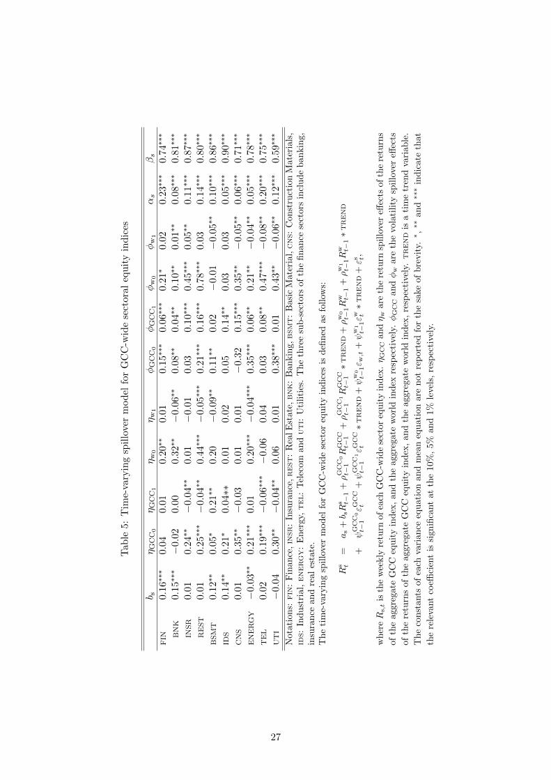
The trend spillover model allows the spillover parameters to increase or decrease with a constant

value. Thus, the spillover parameters may change gradually during the sample period. Table

5 shows the results arising from estimating the trend spillover models for the GCC-wide sector

equity indices. Table 5 is structured in a way similar to Table 3, except that we model the

spillovers to vary across time. Since the estimated time-varying models produce results that are

similar in nature to Table 3, we will not repeat the explanations provided earlier, but focus on

interpreting the return and volatility spillovers.

We find the initial level of the return spillover effect of local shocks (ηGCC0) for the time-

4The hypotheses are: Hypothesis 1: Ho : ηGCC = ηw = 0 (no return spillover effects); Hypothesis 2: Ho :φGCC = φw = 0 (no volatility spillover effects); Hypothesis 3: Ho : ηGCC = φGCC = 0 (no local spillover effects);and Hypothesis 4: Ho : ηw = φw = 0 (no global spillover effects).

11

varying models to be significant for almost all the GCC-wide sector indices, save for, financial

institutions and banking. The trend coefficient of the local shocks (ηGCC1) is mostly insignificant

or negative for the return spillovers. The return spillovers of world shocks (ηw0) are significant

for only the finance sectors (financial institutions, banking and real estate) and the energy

sector, whereas the effect of global shocks on return spillovers has been decreasing, as the trend

coefficient (ηw1) of global shocks is negative and significant. Strong volatility spillover effects are

at play for both the local and global shocks for the GCC-wide sector indices. We find that the

initial level of the volatility spillovers of local shocks (ψGCC0) is significant for nearly all sectors,

as in Table 3, and for all sectors (except for insurance and construction materials, utilities

and industrial goods) and we can observe a positive and significant trend for local volatility

spillovers. Empirically, we find that (ψGCC1) is positive and highly significant, indicating an

increase in the effect of local volatility spillovers on GCC sector indices. Even for some sectors,

particularly for insurance, the initial level of local volatility spillovers negative, and the increase

in the local volatility spillovers throughout the period is 4% and significant, which makes the

local volatility spillovers positive at the end of the period. Applying the time-varying spillover

models to the GCC sector indices, the initial level of the volatility spillovers of world shocks

(ψw0) is significant and positive for all sector indices (except basic materials and industrial

goods). However, there is a significant decrease of this world shocks on volatility spillovers

throughout time. The trend coefficient (ψw1) is negative and significant except for the financial

sectors, indicating the decrease of global shock spillover on the volatility of GCC-wide sector

indices

5 Mean–variance frontiers

The spillover analysis has shown that investors’ decisions to diversify their portfolios across

sectors is mostly driven by the relative importance of idiosyncratic shocks across GCC-wide

sectors. We complement this analysis by investigating the mean–variance frontiers of portfolios

created with all GCC-wide sectoral equities, selected samples of GCC-wide sectoral stocks, and

pure GCC national equities to arrive at the optimal investment portfolio, using the well-known

optimization method proposed by Markowitz (1952).5,6

5See Markowitz (1952) and Moerman (2008) for further details.6The mean-variance portfolio approach proposed by Markowitz (1952) assumes normality, whereas most fi-

nancial series have non-Gaussian distributions and rarely follow (if at all) symmetric distributions. Normalityassumption of the mean variance approach has been challenged by behavioral economists such as Campbell et

12

Figure 1a illustrates the mean–variance frontiers for the three investment opportunity sets

over the period 2005–2008. The selected GCC sector equity indices include: basic materials,

telecom and utilities. These sectors are selected because they have the lowest variance ratios

from local and regional shocks and are mostly driven by own past volatilities. By comparing

the efficiency frontiers of the portfolios created using the sector equity indices with those of

the GCC national equity indices, we are able to determine whether investing in sectoral equity

markets provides more diversification opportunities than investing in stocks across the national

borders. The dotted line is the efficiency frontier for the portfolio composed of selected GCC

sector indices only, the short-dashed line is for the GCC-wide sector indices portfolio and the

long-dashed line is for the national indices portfolio. Figure 1a shows that the portfolio created

with the selected GCC-wide sector indices has a higher efficiency frontier than the portfolio

built with all GCC-wide sector indices as well as the national indices and is confirmed by the

tangency portfolio as shown by the intersection of the capital market line (the solid line) and

the efficient frontier. The tangency portfolio measures the maximum return to risk that can

be obtained by forming portfolios of the assets generating the efficient frontier.7 Comparing

sectoral and national indices, the pure GCC-wide sector equity portfolio has a better portfolio

than the pure nation portfolio in most of the cases.

Figure 1b presents the mean–variance frontiers for the same three investment opportunities

for the period 2008–2012. At first glance, we observe that all efficiency frontiers in Figure 1b

are at lower levels compared to Figure 1a, which is likely due to the spillover effects of the

2008–2009 financial crisis on the GCC markets. The efficiency frontier of the selected sector

equity indices is above those of the national and the GCC sectoral equity indices. This finding

suggests that investors are better off diversifying their investments across different sectors as

opposed to across national markets. Fairly enough, portfolio diversification within the selected

GCC equity sectors creates better opportunities than a portfolio diversified across all the GCC

sector equity markets. Since the selected indices (basic materials, telecom and utilities) are the

least affected by regional and global shocks, we are not quite sure how much of an effect this

may have on the results.

To compare the performance of the portfolios, we calculate the Sharpe ratios8 and present

al. (2001). We thank the anonymous reviewer for bringing this point to our attention.7In selecting the optimal point (i.e., the tangent point reflecting the capital market line and the efficient

portfolio) we considered both US 10-year Treasury bond rate and US 3-month Treasury bill rate available on thelast day of the sample period, which is equal to 1.27% and 0.10%, respectively, in October 2012. In all cases, themore suitable risk-free rate required to find the optimal point was represented by the 3-month Treasury bill rate.

8The Sharpe ratio is a measure of the excess return (or risk premium) per unit of deviation in an investment

13

the results in Table 6. The upper panel of Table 6 reports the average monthly return, the

standard deviation and the Sharpe ratios for the full period (2008–2012). Higher Sharpe ratios

are preferred to lower ones for investment purposes.9 We find the Sharpe ratios are 0.24, 4.83

and 7.34 respectively for the portfolios constructed with purely national equities, all GCC-wide

sector equities and selected GCC-wide sector equities. These confirm our results depicted in

Figures 1a and 1b that investors are better off with a portfolio made up of GCC-wide sector

indices, in particular with basic materials, telecom, and utilities than a portfolio built with GCC

national indices.

The bottom panel of Table 6 reports the Jobson and Korkie (1981) z-statistics matrix,

which is used to test whether the Sharpe ratios are indeed different across portfolios.10 The null

hypothesis is that the Sharpe ratios for any two portfolios are the same, with the alternative

that they are different. In all three cases, considering at the p-values in the parentheses, we

reject the null hypothesis at the 5% critical level, confirming that (i) the selected few GCC-

wide sectors portfolio investment brings highest return to investors per unit of risk, and (ii)

diversifying the portfolio across GCC-wide sector indices bring a better mean–variance outcome

than diversifying the portfolio across national sector indices.

6 Spanning and intersection tests

To further assess the differences in efficiency frontiers that emerge from the three portfolios

created, we empirically estimate the mean–variance spanning and interception tests introduced

by Huberman and Kandel (1987). The basic idea underlying this test is that if an investor holds

an efficient portfolio with a number of assets, X, it is incumbent upon him/her to determine

whether the efficiency frontier improves when a number of assets, say Y , are added to that

portfolio before making such investment. Accordingly, the added assets only add diversification

opportunities to the portfolio if they are not a linear combination of X (i.e. not “spanned”).

asset or a trading strategy, typically referred to as risk (and is a deviation risk measure). The higher the riskpremium per unit of risk for an asset/portfolio the more it is preferred to other assets/portfolios. It is defined as:S = E[R−Rf ]/σ, where R is the asset return, Rf is the return on a benchmark asset (such as the risk free rateof return), E[R−Rf ] is the expected value of the excess of the asset return over the benchmark return and σ isthe standard deviation of the excess of the asset return. Sharp ratios are widely used to rank the performance ofportfolio or mutual fund by investment professionals.

9It should be mentioned that the statistical distribution of the traditional Sharp ratio test is only validasymptotically, but not valid for small samples. Recent studies such as Bai et al. (2005) offer new testingprocedures that are robust to small samples.

10For comparison purposes, we used the performance testing with the Sharpe ratio introduced by Memmel(2003). Although the estimated values have been affected, the rankings have remained unchanged.

14

The mean–variance spanning test is a regression-based test. Since we have two sets of indices,

six dimensional national indices (six GCC national indices) and eight dimensional vectors of

GCC-wide sector indices, we use these as portfolios and ask: whether adding other sector indices

improves the portfolio. Accordingly, we run the following regression

Rs,t = α+ βRi,t + εt (15)

where Rs,t is a N × 1 vector of sector index returns for time t, Ri,t is a K × 1 vector of

national index returns for time t, α is a N ∗ 1 vector of intercepts, β represents the regression

coefficients(N ×K) and εt is the error term by N × 1. The null hypothesis for mean–variance

spanning is therefore

Ho : α = 0, βIk − In = 0 (16)

which is evaluated by using a joint Wald test. The Wald test statistic follows a χ2 distribution

with 2 × N degrees of freedom. A rejection of the null hypothesis signifies that investors can

improve their portfolio by including additional assets, Rs,t. The relation of this to the mean–

variance frontiers is relatively straightforward. Under the null hypothesis, the efficiency frontiers

are equal to each other. If they are not equal, the mean–variance spanning test can be used to

investigate whether they are significantly different from each other. A slightly less restrictive

version of the spanning test is the intersection test, which examines whether the expansion

of the investment opportunities by adding extra indices is important for one specific investor,

whereas the spanning test investigates whether the addition is important for all investors. The

restriction imposed as per the null hypothesis of intersection test is

α− In − κIk = 0 (17)

where κ is the (gross) risk-free interest rate, which is directly related to the risk aversion of the

marginal investor. This test consists of N restrictions and the joint Wald test is χ2 distributed

with N degrees of freedom. We are particularly interested in determining whether investors are

better off by investing in specific industry assets, national assets or both.

The statistical results for both the spanning and the intersection tests are reported in Table 7.

As shown in the upper panel of Table 7, we reject the null hypothesis at the 1% significance level

for both tests irrespective of the sample period considered when the GCC-wide sector indices

15

are added to the portfolio, which implies that addition of GCC-wide sector assets improves

investors’ portfolios. However, when national indices are added instead, the null hypothesis is

accepted for the spanning test but is rejected for the intersection test at the 10% level, indicating

that investors are not better off with this expansion of their portfolios, though these are valid

for a specific risk-free rate or risk aversion parameter.11

Looking at Figures 2a and 2b, we observe similar findings in graphical form. In Figure

2a, the efficiency frontier of the portfolio composed of GCC national and sectoral indices (the

dotted line) is better than the efficiency frontier of the pure national index portfolio (the long-

dashed line) for the period 2005–2008. However, it is not clear whether the portfolio made

up of both sectoral and national indices is better than the portfolio built with sectoral indices

(the short-dashed line) only. The efficiency frontier for the portfolio comprising GCC sectoral

indices is the best at times when the standard deviation of the mean (risk) is very high and

exceeds 3.60%. These times can be characterized by very volatile oil prices and/or very high

geopolitical risk.

In Figure 2b, the efficiency frontier of the portfolio created with sectoral and national indices

is much better than the portfolio with pure national indices for the period 2008–2012, indicating

that investors holding portfolios of GCC national stocks benefit from adding GCC-wide sectoral

assets to their portfolios as well. To complement this result, we investigated whether having

a national and sector portfolio performs better under different constraints. In particular, we

tested for the extreme short- and long positions, but the superior performance of national

plus sectoral indices seems to dominate. As in Figure 2a, we cannot unambiguously rank the

portfolios built with GCC sectoral and national indices and the portfolio made up of GCC

sectoral indices only. Overall, we conclude from the spanning tests and efficiency frontiers

that the portfolio diversification across GCC national indices is not optimal, and adding GCC

sectoral indices brings better opportunities. However, it is somewhat ambiguous whether adding

national indices to portfolio created with purely GCC sectoral indices makes the investors better

off.

11The reported results in Table 7 are based on a risk-free interest rate of 4%. A risk-free rate of 2% is alsoconsidered as a check of the robustness of our results. Although this affects the test statistics, but the overallconclusions remain the same.

16

7 Conclusions

Our objective in this paper was to determine the extent of regional and global equity markets,

return and volatility spillover effects on the GCC equity markets by focusing on the GCC-

wide sectors. We also investigated whether portfolios diversified across the GCC region provide

better opportunities for investors and whether returns are enhanced when portfolios expand to

incorporate other assets. Our results show that GCC-wide sector equity markets are mainly

driven by idiosyncratic shocks. Local and global factors account for less than 50% of the total

variation in sectoral equity return volatility, irrespective of the sector taken into consideration.

For sectors such as basic materials, telecom and utilities, the return volatility is less dependent

on both local and global factors. Additionally, we show that the spillover effects of global shocks

on GCC-wide sector equity returns has been decreasing throughout the period; conversely, the

spillover effect of regional shocks had a positive and increasing effect on the volatility of GCC

sector equity indices. We also find that diversifying a portfolio across GCC sectors yields a

better portfolio than diversifying a portfolio across national GCC equity markets. Portfolios

with selected GCC-wide sector equities are an even better option. This paper offers clear insights

for investors seeking to invest or diversify their portfolio in the GCC equity markets as the GCC

clears away hurdles towards achieving full monetary union, which could eventually mean full

capital market integration.

This paper remains silent on the possibility of including commodities as important elements

for portfolio diversification. In recent years, global trading of major precious metals (e.g., gold,

silver and platinum) have risen significantly and are now being considered by investors in de-

signing prudent risk management and portfolio strategies – see Hammoudeh et al. (2012) for a

recent analysis. Since the economic function of commodities, and hence commodity futures, are

strikingly different from stocks, bonds and other conventional assets (see Gorton and Rouwen-

horst, 2006), the diversification benefits of commodity futures may work well when they are

needed most. In particular, over a long period, as demonestrated by Gorton and Rouwenhorst

(2006), commodity futures returns match equities but with a negative correlation, indicating

that they are an attractive asset class to diversify traditional portfolios of stocks and bonds.

We hope future research will investigate this issue further.

17

References

Adjaoute, K. and Danthine, J.P. (2003). European financial integration and equity returns:A Theory-Based Assessment. In Gaspar, V. et al. (eds), The Transformation of theEuropean Financial System. European Central Bank, Frankfurt.

Al-Khazali, O., Darrat, A.F. and Saad, M. (2006). Intra-regional integration of the GCCstock markets: The role of market liberalization, Applied Financial Economics 16:17,1265–1272.

Bai, Z., Wang, K., Wong, W-K. (2006). Asset Performance Evaluation with the Mean-VarianceRatio. Singapore University Working Paper.

Baele, L., Ferrando, A., Hordahl, P., Krylova, E. and Monnet, C. (2004). Measuring financialintegration in the Euro area, European Central Bank, Occasional Paper No. 14.

Baele, L. (2005). Volatility spillover effects in European equity markets, Journal of Financialand Quantitative Analysis 40, 373–401.

Bashar, Z. (2006). Wild oil prices, but brave stock markets! The case of Gulf CooperationCouncil (GCC) stock markets, Operational Research 6, 145–162.

Bekaert, G. and Harvey, C.R. (1997). Emerging equity market volatility, Journal of FinancialEconomics 43, 29–77.

Bekaert, G., Harvey, C.R. and Ng, A. (2005). Market integration and contagion, Journal ofBusiness 78, 39–69.

Benjelloun, H. (2009). Portfolio diversification: Evidence from Qatar and the UAE, Interna-tional Journal of Economic Issues 2, 9–15.

Berndt, E.R., Hall, B.H., Hall, R.E. and Hausman, J.A. (1974). Estimation and inference innonlinear structural models, Annals of Economics and Social Measurement 3, 653–666.

Bley, J. and Chen, K.H. (2006). Gulf Cooperation Council (GCC) stock markets: The dawnof a new era, Global Finance Journal 17, 75–91.

Bollerslev, T. (1986). Generalized autoregressive conditional heteroskedasticity, Journal ofEconometrics 31, 307–327.

Engle, R.F. (1982). Autoregressive conditional heteroscedasticity with estimates of varianceof United Kingdom inflation, Econometrica 50, 987–1008.

Engle R., Ng, V. and Rothschild, M. (1990). Asset pricing with a factor ARCH covariancestructure: Empirical estimates for treasury bills, Journal of Econometrics 45, 213–237.

Fedorova, E. and Saleem, K. (2010). Volatility spillovers between stock and currency markets:Evidence from emerging eastern Europe, Czech Journal of Economics and Finance 60,519–533.

Fratzscher, M. (2002). Financial market integration in Europe: on the effects of EMU on stockmarkets, International Journal of Finance & Economics 7, 165–193.

Gorton, G. and Rouwenhorst, K.G. (2006). Facts and fantasies about commodity futures,Financial Analysts Journal 62, 47–68.

Hardouvelis, G., Malliaropulos, D. and Priestley, R. (2006). EMU and European stock marketintegration, Journal of Business 79, 365–392.

18

Hammoudeh, S.M. and Aleisa, E. (2004). Dynamic relationship among GCC stock marketsand NYMEX oil futures, Contemporary Economic Policy 22, 250-269

Hammoudeh, S.M. and Choi, K. (2007). Characteristic of permanent and transitory returnsin oil-sensitive emerging stock markets: The case of the GCC countries, Journal of Inter-national Financial Markets, Institutions and Money 17, 231–245.

Hammoudeh, S.M., Yuan, Y. and McAleer, M. (2009). Shock and volatility spillovers amongequity sectors of the Gulf Arab stock markets, Quarterly Review of Economics and Finance49, 829–842.

Hammoudeh, S., Santos, P.A. and Al-Hassan, A. (2012). Downside risk management andVaR-based optimal portfolios for precious metals, oil and stocks, North American Journalof Economics and Finance (in press).

Huberman, S.L. and Kandel, S. (1987). Mean–variance spanning, Journal of Finance 42,873–888.

Jarque, C.M. and Bera, A.K. (1980). Efficient tests for normality, Economics Letters 6, 255–259.

Jobson, J.D. and Korkie, B. (1981). Performance hypothesis testing with the Sharpe andTreynor measures, Journal of Finance 36, 889–908.

Kim, S.J., Moshirian, F. and Wu, E. (2005). Dynamic stock market integration driven by theEuropean monetary union: An empirical analysis, Journal of Banking and Finance 29,2475–2502.

King, M., Sentana, E. and Wadhwani, S. (1994). Volatility and links between national stockmarkets, Econometrica 62, 901–933.

Lin, W., Engle, R.F. and Ito, T. (1994). Do bulls and bears move across borders? Internationaltransmission of stock returns and volatility, Review of Financial Studies 7, 507–538.

Ljung, G.M. and Box, G.E.P. (1978). On a measure of lack of fit in time-series models,Biometrika 65, 297–303.

Memmel, C. (2003). Performance hypothesis testing with the Sharpe ratio, Finance Letters 1,21–23.

Malik, F. and Hammoudeh, S. (2007). Shock and volatility transmission in the oil, US andGulf equity markets, International Review of Economics and Finance 16, 357–368.

Markowitz, H.M. (1952). Portfolio selection, Journal of Finance 7, 77–91.

Moerman, G.A. (2008). Diversification in Euro area stock markets: Country versus industry,Journal of International Money and Finance 27, 1122–1134.

Ng, A. (2000). Volatility spillover effects from Japan and the US to the Pacific-Basin, Journalof International Money and Finance 19, 207–233.

Onour, I. (2007). Impact of oil price volatility on Gulf Cooperation Council stock markets’return, OPEC Review 31, 171–189.

Schwert, G.W. (1989). Why does stock market volatility change over time? Journal of Finance44, 1115–1153.

19

Stulz, R.M. and Karolyi, G.A. (2001). Are financial assets priced locally or globally? In G.M.Constantinides, M. Harris, R.M. Stulz (eds) Handbook of the Economics of Finance, Vol.1, Part B, 975–1020.

Yilmaz, K. (2010). Return and volatility Spillovers among the east Asian equity markets,Journal of Asian Economics 21, 304–313.

20

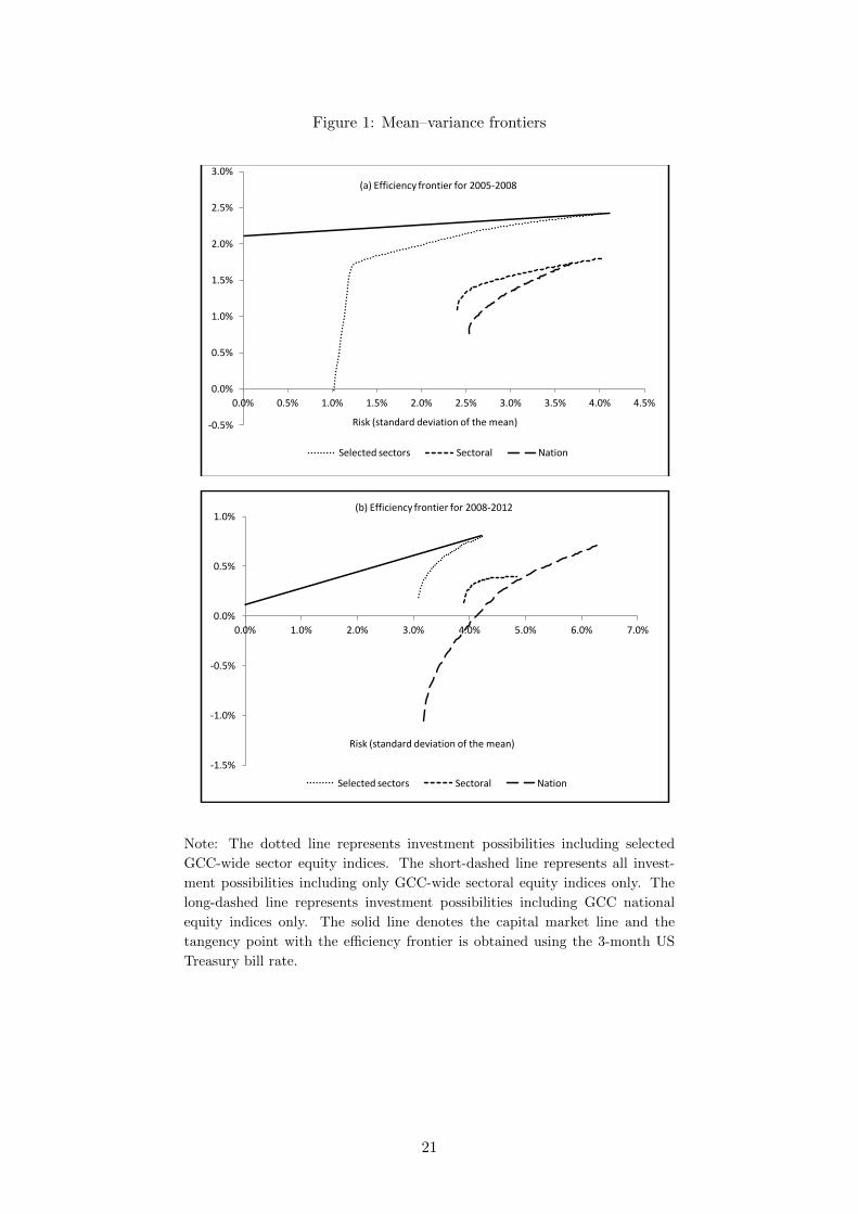
Figure 1: Mean–variance frontiers

-0.5%

0.0%

0.5%

1.0%

1.5%

2.0%

2.5%

3.0%

0.0% 0.5% 1.0% 1.5% 2.0% 2.5% 3.0% 3.5% 4.0% 4.5%

Risk (standard deviation of the mean)

(a) Efficiency frontier for 2005-2008

Selected sectors Sectoral Nation

-1.5%

-1.0%

-0.5%

0.0%

0.5%

1.0%

0.0% 1.0% 2.0% 3.0% 4.0% 5.0% 6.0% 7.0%

Risk (standard deviation of the mean)

(b) Efficiency frontier for 2008-2012

Selected sectors Sectoral Nation

Note: The dotted line represents investment possibilities including selected

GCC-wide sector equity indices. The short-dashed line represents all invest-

ment possibilities including only GCC-wide sectoral equity indices only. The

long-dashed line represents investment possibilities including GCC national

equity indices only. The solid line denotes the capital market line and the

tangency point with the efficiency frontier is obtained using the 3-month US

Treasury bill rate.

21

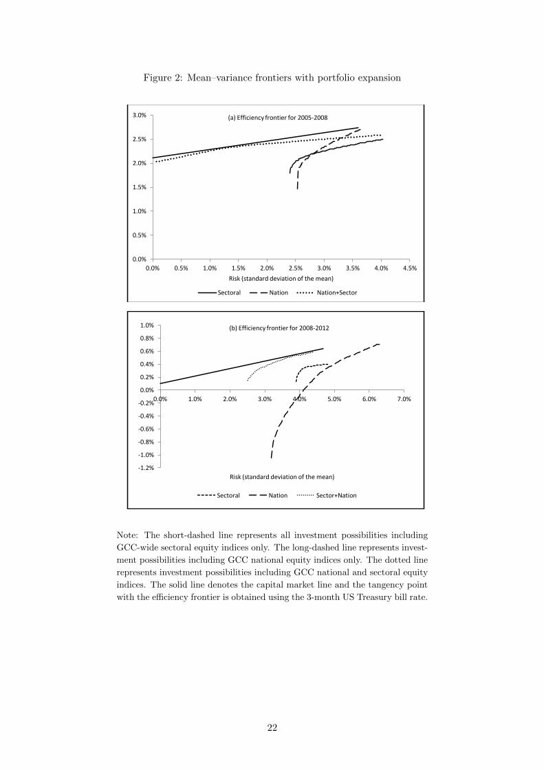
Figure 2: Mean–variance frontiers with portfolio expansion

0.0%

0.5%

1.0%

1.5%

2.0%

2.5%

3.0%

0.0% 0.5% 1.0% 1.5% 2.0% 2.5% 3.0% 3.5% 4.0% 4.5%

Risk (standard deviation of the mean)

(a) Efficiency frontier for 2005-2008

Sectoral Nation Nation+Sector

-1.2%

-1.0%

-0.8%

-0.6%

-0.4%

-0.2%

0.0%

0.2%

0.4%

0.6%

0.8%

1.0%

0.0% 1.0% 2.0% 3.0% 4.0% 5.0% 6.0% 7.0%

Risk (standard deviation of the mean)

(b) Efficiency frontier for 2008-2012

Sectoral Nation Sector+Nation

Note: The short-dashed line represents all investment possibilities including

GCC-wide sectoral equity indices only. The long-dashed line represents invest-

ment possibilities including GCC national equity indices only. The dotted line

represents investment possibilities including GCC national and sectoral equity

indices. The solid line denotes the capital market line and the tangency point

with the efficiency frontier is obtained using the 3-month US Treasury bill rate.

22

Table 1: Descriptive statistics

Mean STD Skew Kurt Q(1) Q(4) Q†(1) Q†(4)

FIN 0.10 6.48 –0.87 2.37 0.19∗∗∗ 0.11∗∗∗ 0.12∗∗ 0.14∗∗∗

BNK -0.01 2.12 –1.45 10.23 0.14∗∗∗ 0.11∗∗ 0.21∗∗∗ 0.13∗∗∗

INSR -0.02 2.45 0.12 2.43 0.09∗∗∗ 0.14∗∗∗ 0.14∗∗∗ 0.21∗∗∗

REST -0.02 6.02 –0.32 7.21 0.21∗∗∗ −0.05 0.13∗∗∗ 0.05∗∗

BSMT 0.05 5.21 –2.21 5.44 0.03∗ 0.12∗∗ 0.18∗∗∗ 0.23∗∗∗

IDS 0.06 3.56 –1.01 4.59 0.17∗∗∗ 0.01∗∗∗ 0.12∗∗∗ 0.04∗∗∗

CNS –0.02 3.91 –0.48 4.91 0.11∗∗ −0.03 0.20∗∗ 0.15∗∗∗

ENERGY –0.12 4.11 –0.45 2.81 0.12 0.01 0.21∗∗∗ 0.12∗∗∗

TEL 0.05 3.04 –0.15 3.51 −0.11∗ 0.03 0.15∗∗∗ 0.15∗∗∗

UTI 0.03 4.44 –1.04 4.99 −0.05 −0.04 0.16∗∗∗ 0.11∗∗∗

GCC –0.04 4.01 –0.96 4.41 0.06∗∗∗ −0.05 0.17∗∗∗ 0.13∗∗∗

WORLD 0.02 3.05 –1.21 15.31 −0.11∗∗ 0.13∗∗∗ 0.16∗∗∗ 0.09∗∗∗

Notations: FIN: Finance, INSR: Insurance, REST: Real Estate, BNK: Banking, BSMT:

Basic Material, CNS: Construction Materials, IDS: Industrial, ENERGY: Energy, TEL:

Telecom and UTI: Utilities. The three sub-sectors of the finance sectors include bank-

ing, insurance and real estate.

The table reports the summary statistics for the weekly returns (in %) of the GCC-

wide sector, aggregate GCC and aggregate world equity indices. The following statis-

tics are reported: mean, standard deviation (STD), skewness (Skew), kurtosis (Kurt),

autocorrelations of order 1 and 4 (Q(1) and Q(4)) and autocorrelations of the squared

time series of order 1 and 4 (Q†(1) and Q†(4)). ∗, ∗∗ and ∗∗∗ indicate that the Ljung

and Box (1978) test statistic is significant at the 10%, 5% and 1% levels, respectively.

23

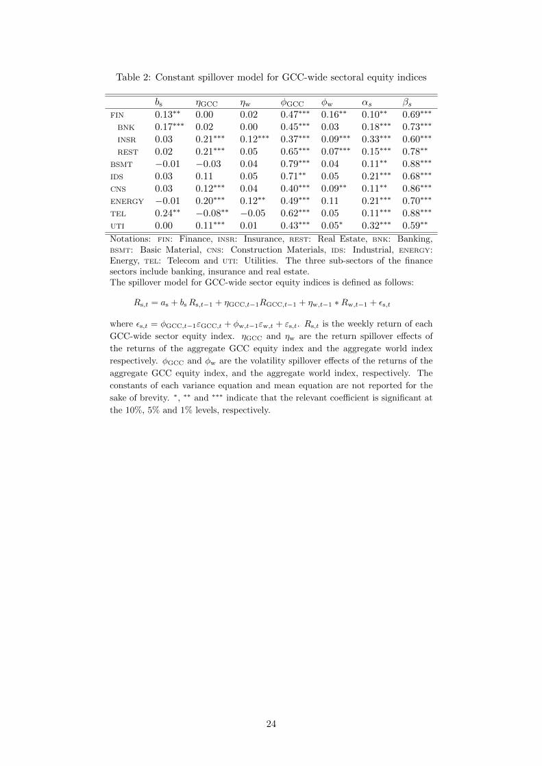
Table 2: Constant spillover model for GCC-wide sectoral equity indices

bs ηGCC ηw φGCC φw αs βsFIN 0.13∗∗ 0.00 0.02 0.47∗∗∗ 0.16∗∗ 0.10∗∗ 0.69∗∗∗

BNK 0.17∗∗∗ 0.02 0.00 0.45∗∗∗ 0.03 0.18∗∗∗ 0.73∗∗∗

INSR 0.03 0.21∗∗∗ 0.12∗∗∗ 0.37∗∗∗ 0.09∗∗∗ 0.33∗∗∗ 0.60∗∗∗

REST 0.02 0.21∗∗∗ 0.05 0.65∗∗∗ 0.07∗∗∗ 0.15∗∗∗ 0.78∗∗

BSMT −0.01 −0.03 0.04 0.79∗∗∗ 0.04 0.11∗∗ 0.88∗∗∗

IDS 0.03 0.11 0.05 0.71∗∗ 0.05 0.21∗∗∗ 0.68∗∗∗

CNS 0.03 0.12∗∗∗ 0.04 0.40∗∗∗ 0.09∗∗ 0.11∗∗ 0.86∗∗∗

ENERGY −0.01 0.20∗∗∗ 0.12∗∗ 0.49∗∗∗ 0.11 0.21∗∗∗ 0.70∗∗∗

TEL 0.24∗∗ −0.08∗∗ −0.05 0.62∗∗∗ 0.05 0.11∗∗∗ 0.88∗∗∗

UTI 0.00 0.11∗∗∗ 0.01 0.43∗∗∗ 0.05∗ 0.32∗∗∗ 0.59∗∗

Notations: FIN: Finance, INSR: Insurance, REST: Real Estate, BNK: Banking,BSMT: Basic Material, CNS: Construction Materials, IDS: Industrial, ENERGY:Energy, TEL: Telecom and UTI: Utilities. The three sub-sectors of the financesectors include banking, insurance and real estate.The spillover model for GCC-wide sector equity indices is defined as follows:

Rs,t = as + bsRs,t−1 + ηGCC,t−1RGCC,t−1 + ηw,t−1 ∗Rw,t−1 + εs,t

where εs,t = φGCC,t−1εGCC,t + φw,t−1εw,t + εs,t. Rs,t is the weekly return of each

GCC-wide sector equity index. ηGCC and ηw are the return spillover effects of

the returns of the aggregate GCC equity index and the aggregate world index

respectively. φGCC and φw are the volatility spillover effects of the returns of the

aggregate GCC equity index, and the aggregate world index, respectively. The

constants of each variance equation and mean equation are not reported for the

sake of brevity. ∗, ∗∗ and ∗∗∗ indicate that the relevant coefficient is significant at

the 10%, 5% and 1% levels, respectively.

24

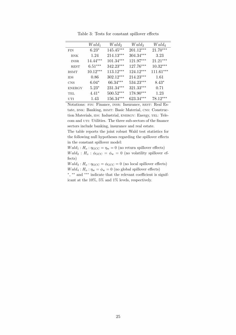
Table 3: Tests for constant spillover effects

Wald1 Wald2 Wald3 Wald4FIN 6.23∗ 145.45∗∗∗ 201.12∗∗∗ 21.70∗∗∗

BNK 1.24 214.13∗∗∗ 304.34∗∗∗ 3.23INSR 14.44∗∗∗ 101.34∗∗∗ 121.97∗∗∗ 21.21∗∗∗

REST 6.51∗∗∗ 342.23∗∗∗ 127.76∗∗∗ 10.32∗∗∗

BSMT 10.12∗∗∗ 113.12∗∗∗ 124.12∗∗∗ 111.61∗∗∗

IDS 0.86 302.12∗∗∗ 214.23∗∗∗ 1.61CNS 6.04∗ 66.34∗∗∗ 534.23∗∗∗ 8.43∗

ENERGY 5.23∗ 231.34∗∗∗ 321.33∗∗∗ 0.71TEL 4.41∗ 500.52∗∗∗ 178.90∗∗∗ 1.23UTI 1.43 156.34∗∗∗ 623.34∗∗∗ 78.12∗∗∗

Notations: FIN: Finance, INSR: Insurance, REST: Real Es-

tate, BNK: Banking, BSMT: Basic Material, CNS: Construc-

tion Materials, IDS: Industrial, ENERGY: Energy, TEL: Tele-

com and UTI: Utilities. The three sub-sectors of the finance

sectors include banking, insurance and real estate.

The table reports the joint robust Wald test statistics for

the following null hypotheses regarding the spillover effects

in the constant spillover model:

Wald1 : Ho : ηGCC = ηw = 0 (no return spillover effects)

Wald2 : Ho : φGCC = φw = 0 (no volatility spillover ef-

fects)

Wald3 : Ho : ηGCC = φGCC = 0 (no local spillover effects)

Wald4 : Ho : ηw = φw = 0 (no global spillover effects)∗, ∗∗ and ∗∗∗ indicate that the relevant coefficient is signif-

icant at the 10%, 5% and 1% levels, respectively.

25

Table 4: Variance ratios: local and global shocks

Local STD Global STD

FIN 0.38 0.08 0.12 0.04BNK 0.34 0.04 0.10 0.03INSR 0.30 0.11 0.25 0.04REST 0.38 0.10 0.16 0.08

BSMT 0.22 0.06 0.02 0.04IDS 0.36 0.08 0.06 0.04CNS 0.26 0.08 0.16 0.06ENERGY 0.33 0.05 0.17 0.04TEL 0.20 0.13 0.6 0.03UTI 0.17 0.09 0.09 0.06

Notations: FIN: Finance, INSR: Insurance, REST:Real Estate, BNK: Banking, BSMT: Basic Material,CNS: Construction Materials, IDS: Industrial,ENERGY: Energy, TEL: Telecom and UTI: Utilities.The three sub-sectors of the finance sectors includebanking, insurance and real estate.The table reports the mean and the standard devi-ation (STD) of the sector equity indices’ varianceratios. The variance ratio of the spillover effect ofboth local aggregate GCC equity index and thesector equity indices is formulated as:

V RGCCs,t =

φ2GCC,t−1

ε2GCC,t

hs,tand V Rw

s,t =φ2w,t−1ε

2w,t

hs,t,

where hs,t = σ2s,t + φ2GCC,t−1σ

2GCC,t + φ2w,t−1σ

2w,t.

∗, ∗∗ and ∗∗∗ indicate that the relevant coefficient

is significant at the 10%, 5% and 1% levels, respec-

tively.

26

Tab

le5:

Tim

e-va

ryin

gsp

illo

ver

mod

elfo

rG

CC

-wid

ese

ctor

aleq

uit

yin

dic

es

b sη G

CC

0η G

CC

1η w

0η w

1φGCC

0φGCC

1φw

0φw

1αs

βs

FIN

0.16∗∗∗

0.0

40.

010.

20∗∗

0.01

0.15∗∗∗

0.0

6∗∗∗

0.2

1∗0.0

20.

23∗∗∗

0.7

4∗∗∗

BNK

0.15∗∗∗

−0.0

20.0

00.

32∗∗

−0.

06∗∗

0.0

8∗∗

0.0

4∗∗

0.1

0∗∗

0.0

1∗∗

0.0

8∗∗∗

0.8

1∗∗∗

INSR

0.01

0.24∗∗

−0.0

4∗∗

0.0

1−

0.01

0.03

0.1

0∗∗∗

0.4

5∗∗∗

0.0

5∗∗

0.11∗∗∗

0.8

7∗∗∗

REST

0.0

10.

25∗∗∗−

0.0

4∗∗

0.4

4∗∗∗−

0.05∗∗∗

0.21∗∗∗

0.1

6∗∗∗

0.7

8∗∗∗

0.0

30.

14∗∗∗

0.8

0∗∗∗

BSMT

0.12∗∗

0.0

5∗0.2

1∗∗

0.2

0−

0.09∗∗

0.11∗∗

0.0

2−

0.0

1−

0.05∗∗

0.10∗∗∗

0.8

6∗∗∗

IDS

0.14∗∗

0.2

1∗0.0

4∗∗

0.0

10.

020.

050.1

4∗∗

0.0

30.0

30.

05∗∗∗

0.9

0∗∗∗

CNS

0.01

0.35∗∗

−0.0

30.

010.

01−

0.3

20.1

5∗∗∗

0.3

5∗∗−

0.05∗∗

0.0

6∗∗∗

0.7

1∗∗∗

ENERGY−

0.03∗∗

0.2

1∗∗∗

0.0

10.

20∗∗∗−

0.04∗∗∗

0.3

5∗∗∗

0.0

6∗∗

0.2

1∗∗−

0.04∗∗

0.0

5∗∗∗

0.7

8∗∗∗

TEL

0.02

0.19∗∗∗−

0.0

6∗∗∗−

0.06

0.0

40.

030.0

8∗∗

0.4

7∗∗∗−

0.08∗∗

0.2

0∗∗∗

0.7

5∗∗∗

UTI

−0.

040.

30∗∗−

0.0

4∗∗

0.06

0.01

0.38∗∗∗

0.0

10.4

3∗∗−

0.06∗∗

0.1

2∗∗∗

0.5

9∗∗∗

Not

atio

ns:

FIN

:F

inan

ce,IN

SR

:In

sura

nce

,REST

:R

ealE

state

,BNK

:B

an

kin

g,BSM

T:

Basi

cM

ate

rial,

CNS:

Con

stru

ctio

nM

ate

rials

,ID

S:

Ind

ust

rial

,ENERGY

:E

ner

gy,TEL:

Tel

ecom

an

dUTI:

Uti

liti

es.

Th

eth

ree

sub

-sec

tors

of

the

fin

an

cese

ctors

incl

ud

eb

an

kin

g,

insu

ran

cean

dre

ales

tate

.T

he

tim

e-va

ryin

gsp

illo

ver

mod

elfo

rG

CC

-wid

ese

ctor

equ

ity

indic

esis

defi

ned

as

foll

ows:

Rs t

=as

+b sR

s t−1

+ρGCC

0t−

1R

GCC

t−1

+ρGCC

1t−

1R

GCC

t−1∗

TREND

+ρw

0t−

1R

w t−1

+ρw

1t−

1R

w t−1∗

TREND

+ψGCC

0t−

1εG

CC

t+ψGCC

1t−

1εG

CC

t∗

TREND

+ψw

0t−

1ε w,t

+ψw

1t−

1εw t∗

TREND

+εs t,

wh

ereR

s,t

isth

ew

eekly

retu

rnof

each

GC

C-w

ide

sect

or

equ

ity

ind

ex.η G

CC

an

dη w

are

the

retu

rnsp

illo

ver

effec

tsof

the

retu

rns

ofth

eag

greg

ate

GC

Ceq

uit

yin

dex

,an

dth

eaggre

gate

worl

din

dex

resp

ecti

vely

.φGCC

an

dφw

are

the

vola

tili

tysp

illo

ver

effec

ts

ofth

ere

turn

sof

the

aggr

egat

eG

CC

equ

ity

ind

ex,

an

dth

eaggre

gate

worl

din

dex

,re

spec

tive

ly.

TREND

isa

tim

etr

end

vari

ab

le.

Th

eco

nst

ants

ofea

chva

rian

ceeq

uat

ion

and

mea

neq

uati

on

are

not

rep

ort

edfo

rth

esa

keof

bre

vit

y.∗ ,∗∗

an

d∗∗∗

ind

icate

that

the

rele

vant

coeffi

cien

tis

sign

ifica

nt

atth

e10%

,5%

an

d1%

leve

ls,

resp

ecti

vely

.

27

Table 6: Performance tests and Z-statistics

A. Performance Tests

Mean STD Sharpe Ratio(%)

Nation 0.02 8.12 0.24Sector 0.30 6.21 4.83Selected Sector 0.36 4.90 7.34

B. Z-statistics

Nation Sector Selected SectorNation –Sector 2.99 –

(0.0011) –Selected Sector 3.34 2.20 –

(0.0003) (0.016) –

The mean and standard deviation (STD) of monthly returns and

Sharpe ratios are all in percentages. The Nation (Sector) row rep-

resents the mean and standard deviation of the monthly return and

Sharpe ratio for when the portfolio is diversified across GCC na-

tional (sectoral) indices only. Selected Sector equity indices are made

up from selected sector equity indices. Jobson-Korkie z-statistics are

reported in the lower panel via a matrix. For example, 2.99 is the

Jobson-Korkie z-statistic when we test if the Sharpe ratio of the port-

folio, made up from GCC national equity indices (Nation) and the

Sharpe ratio of the portfolio, made up from GCC sectoral equity in-

dices (Sector) are different from each other (H0 : SHARPENation =

SHARPESector). p-values are in parentheses.

28

Table 7: Spanning and intersection tests

A. Adding GCC-wide Sector Indices

2005–2008 2008–2011 2005–2011

Spanning 0.000 0.001 0.000Intersection 0.000 0.010 0.001

B. Adding National Indices

Spanning 0.141 0.171 0.92Intersection 0.062 0.081 0.094

This table presents the p-values of the mean–variance span-

ning and intersection tests, as described in the text. The null

hypothesis of the spanning test is that there is no investor

who can significantly improve his/her portfolio by including

the added indices. The intersection test tests the null hypoth-

esis that one specific investor (measured by his/her risk aver-

sion parameter or the risk-free rate) cannot significantly im-

prove his/her portfolio by including the added assets. We used

an interest rate of 4% per annum for this test, but unreported

results show that the results are robust to this assumption.

29