Munich Personal RePEc Archive - uni-muenchen.de · Manacorda, Manning and Wadsworth (2012) propose...

MPRAMunich Personal RePEc Archive

The impact of immigration on the labourmarket: Evidence from 20 years ofcross-border migration to Argentina

Diego Battiston

London School of Economics, CEP

2013

Online at https://mpra.ub.uni-muenchen.de/52424/MPRA Paper No. 52424, posted 24 December 2013 06:44 UTC

http://mpra.ub.uni-muenchen.de/

https://mpra.ub.uni-muenchen.de/52424/

This paper studies the effects of immigration on the wages of Argentinean native

workers over the period 1993-2012. I use a novel micro-dataset which combines

household surveys from Argentina and six other Latin American countries.

Immigration from these six countries accounts for 95% of the total immigration

from Latin American countries. The empirical strategy identifies the effects of

the labour supply variation using the “national approach” from Borjas (2003) and

a reduced form equation obtained within a CES framework. In order to account

for demand/pull shocks, I propose a set of instruments based on labour market

conditions in immigrants’ home countries. An alternative specification also

explores the hypothesis of heterogeneous impact by country of origin. Overall,

findings show a significant negative impact of immigration on wages. IV

estimates suggest that OLS results are a lower bound for the (partial) causal

effect. Thus, if confounding demand factors exist, they bias the results toward

zero.

During the last years there has been an active debate about the effects of

immigration on the labour market, particularly on the impact on the wage structure

of native population. Borjas (2003) develops a framework to account for such impact

evaluating immigration as a labour supply shock for workers with similar

characteristics. In two recent works, Manacorda, Manning and Wadsworth (2012)

and Ottaviano and Peri (2005) extend the standard setting to allow for imperfect

substitution between migrants and natives. Both papers find evidence of imperfect

substitution and a low impact of immigration on the wage structure of natives for

the UK and the US. Peri and Sparber (2009) conclude that the lack of substitution

between natives and immigrants could be driven by differences in linguistic abilities

and other cultural dissimilarities. A natural follow-up question arises about the

1 I thank Alan Manning, Soledad Giardili and Guillermo Cruces for helpful comments and

suggestions. I also thank Pablo Gluzmann for helpful support with SEDLAC database.

PRELIMINAR VERSION.

2

effects of immigration in countries with higher rates of immigrants’ assimilation and

fewer differences with their home cultures.

Most of the academic debate about immigration has been focused on traditional

corridors like Mexico-US and other South-North corridors. However, South-South

migration has interesting characteristics and may contribute to the debate about the

impact of immigration. Particularly, cross-border migration to Argentina has not

received much attention in the academic literature. Few descriptive works exists

about immigration in this corridor and no work attempted to estimate the causal

impact on the local labour market. The magnitude of migration flows to Argentina

was significant in the last decades. Jachimowicz (2006) estimates an average inflow

of 15.000 permanent migrants per year between 1995 and 2002. According to the

2010 census, approximately 5% of the total population in Argentina is foreign and

81% of this group migrated from Latin American countries. In some areas this value

increases notably, for instance, foreign population in Buenos Aires city represents

13.2% of total population.

There are some characteristics that make this corridor an interesting case of

analysis. First, all the countries in the region (with few exceptions) have a common

language and cultural barriers seem to be lower than in other corridors. Moreover,

this characteristic has a methodological advantage: Dustmann and Fabbri (2003)

and Dustmann and Preston (2011) conclude that language differences reduce the

ability of immigrants to find a job that suits with their education and experience.

The “downgrading effect” produced by language violates the identification

assumptions of common approaches. Second, legal barriers to immigration are much

weaker than the case of US or UK policies and illegal immigration is presumably

lower. Third, during the last decades, most immigrants arrived from a small group

of countries. Finally, the composition of immigrant population by country of origin

has changed drastically over time.

This paper contributes to the existing literature in different ways: First, it is the

first empirical work addressing the impact of immigration on the labour market in

this important corridor. I address specific problems and characteristics related to the

South- South corridors, for instance, internal migration and native emigration are

recognised as confounding factors of the causal impact. Second, in order to isolate

supply shocks from demand/pull factors, I propose a set of instrumental variables

using a novel micro-database with harmonized socioeconomic information from six

LAC countries. These countries accounts for 95% of recent Latin American migration

toward Argentina. This paper also explores the hypothesis that the effect on wages

varies by country of origin under imperfect substitution among immigrants. This is

particularly interesting in the case of Argentina since the composition of

immigration has been changing during the last 20 years. Indeed, some countries like

3

Paraguay, Bolivia and Peru have notably increased their share in total Latin-

American immigrant population.

The rest of the paper is organized as follows. Section 2 discusses the CES

framework and the wage equations for natives and immigrants. Section 3 describes

Data. Section 4 briefly summarizes the evolution of immigrant flows to Argentina

and discusses some facts and evidence of this process. Section 5 discusses the

baseline empirical setting and alternative identification strategies like IV and

geographical stratification. Section 6 presents all the results and Section 7

summarizes the main conclusions of this work.

Consider a version of the model proposed in Manacorda, Manning and Wadsworth

(2012) which in turn is based on the model in Card and Lemieux (2001). Firms

produce using a neoclassical production function that combines labour and capital.

For simplicity, assumes that it can be represented by a Cobb-Douglas function with

neutral technological change:

(1) 1

t t t tY A K L

Capital can be assumed either fixed in the short run or endogenous in the long run

but exogenous from the point of view of a firm deciding the composition of the bundle

of labour inputs. Labour is a composite input that aggregates different skill groups

(indexed by e) using a CES technology:

(2)

1

1

E

t et ete

L L

where 1 1t is the usual normalization for the relative efficiency parameters.

Substitution between different education groups is measured by the elasticity of

substitution 1/ (1 )E . Similarly, et

L is composited by different experience groups

a=1,..,A.

(3)

1

1

A

et ea eata

L v L

, 1,..., ; 1,...,e E a A

The relative efficiency parameter eav is assumed to be time invariant and 1ev is

normalized to one. The elasticity of substitution across experience groups is equal to

4

1/ (1 )A . Finally, native and immigrant sub-population are (potentially)

imperfect substitutes:

(4) 1

eat neat eat meatL L b L

, 1,..., ; 1,...,e E a A

where nL is the native sub-population and

nL is the immigrant sub-population and

parameter eat

b accounts for differences in efficiency units provided by immigrants.

Substitution between natives and immigrants is equal to 1/ (1 )M . Assuming

competitive markets, wages are equated to marginal productivity for each type of

worker.

(5) 1

neat t et t et ea eat neatw Y L L v L L

(6) 1

meat t et t et ea eat eat meatw Y L L v L b L

The empirical version of equations (5) and (6) can be easily derived, consider for

example the log-transformation of (5):

(7) log log ( )log ( )log ( 1)logneat t et ea t et eat neat

w Y v L L L L

where log , etc. Even though the terms , tY ,

et and ea

v can be absorbed by a

set of dummies and interactions, equation (7) cannot be directly estimated by OLS

since for example eat

L only can be calculated when there is an available estimation of

δ. Manacorda, Manning and Wadsworth (2012) propose an econometric procedure to

estimate the structural version of a similar model in several steps, that approach is

briefly discussed in section 5 but beyond the scope of this paper.2

This simple CES framework is the base of the empirical strategy discussed in

Section 5 and is has been widely used in recent literature because it allows for a high

degree of flexibility in terms of substitution across education and age dimension but

only imposes a low number of parameters to estimate. The main disadvantage of the

nested CES approach is that substitution within education or age dimension is

constant, for instance, the substitution degree between workers with high and

medium education is assumed to be the same than substitution between workers

with high and low education. Section 5 describes an empirical strategy to identify

2 An analogous wage equation to (7) holds for immigrants under the assumption of no market

discrimination against them. However, if this (negative) discrimination premium is assumed

to be proportional to the counterfactual wage in a scenario without discrimination, a simple

reinterpretation of the constant term can accommodate this problem. In other words,

log logm D , where D is the proportional discrimination adjustment.

5

some aspects of this model without relying on the structural estimation of all the

parameters.

The basic model assumes that immigrants are perfect substitutes independently

of the country of origin. There are many reasons to believe that migrants from

different countries are not perfect substitutes. First, countries of origin are

heterogeneous in terms of culture, education quality, and other unobserved variables.

Second, even though this model takes into account differences in education and

experience, selection in unobservables (Borjas, 1987) is a potential source of

heterogeneity between workers from different countries. For example, sorting across

sectors seems to be very different for workers from different countries, indicating

some unobserved differences between migrants with same education/experience but

different nationality (Patel and Vella, 2007, Toussaint-Comeau, 2007).

To allow for imperfect substitution across nationalities, I assume that immigrant

population can be aggregated by means of a CES technology with substitution3

1/ (1 )J :

(8)

1

1

J

meat jmeat jmeatj

L c L

with 1meatc normalized to one. In this case, theoretical wages also varies within cells

with the supply of workers from countries of origin j=1,…,J. The reason to allow jmeatc

to vary along time is that immigration waves from the same country can change in

terms of efficiency units because different economic or legal conditions in origin and

destination can change the self-selection patterns (Longhi and Rokicka, 2012). First

order conditions, assuming no discrimination against immigrants, imply that wages

for each education-age-immigrant group are given by:

(9) 1

jmeat t t et t et ea eat eat meat jmeat jmeatw Y L L L a L b L c L

Although there is an extensive literature estimating the impact of immigration

on wages, there are no attempts to identify heterogeneity of this impact by country

of origin. The only exception (to my knowledge) is Bratsberg et al. (2011) who use a

3 Alternatively, it can be assumed that 1

1( )

M

eat neat eat meatmL L b L

with m indexing the

immigrant nationality. This specification means that substitution between natives and

immigrants is the same than substitution between two groups of immigrants.

6

panel dataset from Norway to test if immigration from Nordic and high income

countries had a different effect than immigration from developing countries.

The main source of data for this paper is the Socioeconomic Database for Latin

America and the Caribbean (SEDLAC), jointly developed by CEDLAS at the

Universidad Nacional de La Plata (Argentina) and the World Bank’s LAC poverty

group (LCSPP). This database contains information on more than 200 official

household surveys in 25 LAC countries. All variables in SEDLAC are constructed

using consistent criteria across countries and years, and identical programming

routines 4 . In this paper I use micro-data for Argentina and a set of six Latin

American countries that account for more than 95% of immigrant flows from the

region. Most of the analysis is done using the Argentinean sub-sample but the IV

strategy uses information at the level of the country of origin of the immigrants.

The data covers the period 1993-2012. For comparison purposes, I restrict the

sample for each country to those areas covered by the national household survey in

the whole period of analysis. In the case of Argentina, only 18 large urban areas had

information on immigration in the 1993 survey and I restrict subsequent years to

the same geographical coverage.5 Micro-data for Argentina in the SEDLAC database

corresponds to the Encuesta Permanente de Hogares officially carried out by the

Instituto Nacional de Estadística y Censos (INDEC) since the 1980s. In the case of

Brazil I exclude Rural-North areas included since 2004 and I only use urban areas

from Uruguay since rural areas were added in 2006. The case of Bolivia is more

restrictive since only regional capital cities and the city of El Alto, were covered in

1993 and I restrict the sample to these cities for all the available years. Since there

is no available information for Peru before 1997, I use the 10% census IPUMS extract

for 1993. To keep consistency and comparability across years I harmonize the Census

data applying the same methodology and definitions than SEDLAC database.

Unfortunately, income information is not available for Peru 1993 Census data. Table

1 reports data availability for each year and country included in the sample.

It is worth mentioning that the official EPH survey from Argentina was carried

out in two rounds (May and October) until 2003 but SEDLAC database only contains

the October round for that period. On the other hand, SEDLAC micro-data is

4 A detailed description of the methodology and definitions is available at

http://sedlac.econo.unlp.edu.ar/eng/methodology.php 5 The geographical coverage of the survey was extended from 15 urban areas in 1992 to 31

urban areas in 2003. Nevertheless, the 18 areas included in 1993 account for 85% of the

population in the latest years of the survey (which represents 70% of the total urban

population in the country). On the other hand, the share of urban population is estimated to

be 87%.

7

available for both semesters since 20036. In order to keep consistency and exploit all

the information available, I process and harmonize the May round of the EPH for

each year within the period 1993-2003 using the same definitions and methodology

than the SEDLAC database.

Micro-data available for the covered period

Another difference between SEDLAC and the data I use in this work is that the

former does not have detailed information on immigration. For that purpose, I

identify immigrants by country of origin and year of arrival from the original EPH

survey and match this information at individual level with the SEDLAC dataset.

Argentina is a country with a long tradition in immigration inflows. European

mass migration during the late 19th and the early 20th century has been considered

among the largest population inflows experienced by a country (Hatton and

Williamson, 1998). During that period Argentina implemented a set of active policies

to incentive immigration. For instance, the Constitution from 1853 prohibited any

barrier, tax or quota to European immigration. Census records show that the

immigrant population increased from 210 thousands to 2.3 million between 1869 and

1914. By that time, the immigrant share over total population reached 30%.

European inflows started to decline after 1914 and virtually stopped in the late

1950s after a short period of high inflows during the 5 years following the Second

World War (Solimano, 2003).

In the last decades, immigration from Latin American countries, particularly

from Bolivia, Chile, Paraguay, Peru and Uruguay, shifted the older European waves.

As discussed in Pacceca and Courtis (2008) there was an important shift in the

destination of Latin American immigrants before and after the 60s. The inflows of

6 There is a methodological change from 2003 and now the survey is conducted over the whole

year and reported in quarterly sub-samples. SEDLAC database groups the 4 subsamples in

first and second semester respectively.

Country/Year 1993 1994 1995 1996 1997 1998 1999 2000 2001 2002 2003 2004 2005 2006 2007 2008 2009 2010 2011 2012

Argentina x x x x x x x x x x x x x x x x x x x x

Bolivia x x x x x x x x x x x x x

Brazil x x x x x x x x x x x x x x x x

Chile x x x x x x x x

Paraguay x x x x x x x x x x x x

Peru x x x x x x x x x x x x x x x

Uruguay x x x x x x x x x x x x x x x x x

Notes: Argentina : Each year pool first and second semester data except for 1993 and 2012 with only one semester available.

Bolivia : 2003 and 2004 unified survey. Chile : 1992 survey also included in the sample. Peru : 1993 correspond to the IPUMS

10% census sample. Uruguay : 1992 survey also included

8

workers before 1960 were concentrated in rural areas where the labour supply had

dropped due to internal migration toward urban areas. Immigrants usually moved

between locations and most of them frequently returned to their home countries.

After 1960, most of the immigrants arrived to large urban areas and stay

permanently. Political instability during the 70’s and 80’s in Uruguay and Chile7

suddenly increased the share of immigrants from these countries whereas inflows

from Bolivia and Paraguay have been continuously increasing since the 50s and in

the case of Peru since the 80s in (Maurizio, 2007).

During the last two decades, according with Census data, the number of

immigrants born in Bolivia, Brazil, Chile, Paraguay, Peru and Uruguay increased

from 817 thousands in 1991 to 1.4 million in 2010 (Castillo and Gurrieri, 2012). This

increase was not monotonic along the period neither homogenous across home

countries. The economic crisis in 2001 temporarily reduced the migration inflows,

accelerated the number of immigrants who returned home and increased the

emigration of native population. After 2003 there is an important increase in the

number of immigrants from Bolivia, Brazil, Paraguay and Peru although the number

of Uruguayan remains stable and the number of Chileans decreases. Overall,

immigration from these six countries increased 39% between 2001 and 2010. Figure

A1 in the appendix shows the distribution of immigrants by country of origin in

South America according to the last Census. The figure also plots the geographical

location of the 18 urban areas covered in the Argentinean sample.

Beyond the after-crisis recovery of the Argentinean economy, the large increase

in immigration during the last decade also coincided with the introduction of a new

immigration law in 2004 (Law 25,871). The new law shortens the length of time

required to obtain the Argentinean citizenship or the permanent residence

permission, relaxes the requisites to obtain it and also legalizes the situation of

thousands of immigrants who were not formally registered as workers. The previous

immigration law dated from 1981 (during the military government) and was more

restrictive, but in practice, the barriers to immigration were relatively low. The lack

of frontier controls, the high level of informality in the labour market, regular

amnesty laws (in 1974, 1984, 1992 and 1994) and the 1998 bilateral migration

agreements with Bolivia and Peru, contributed to the low effectiveness of the 1981

law8.

7 Political instability characterized the whole region during these decades but the military

coups occurred in 1973 in Uruguay and Chile were highly correlated with the sudden increase

in the emigration rates from these countries (see for example Pellegrino and Vigorito, 2005) 8 For instance, before 1994 it was possible for any immigrant to change the residence status

from “temporary“ (tourists for example) to “permanent” without leaving the country. After

1994 this process was more regulated although it was still feasible to remain in the country

as a worker with a temporary permission. A whole analysis of the immigration laws since

1876 can be found in Pacecca and Courtis (2008).

9

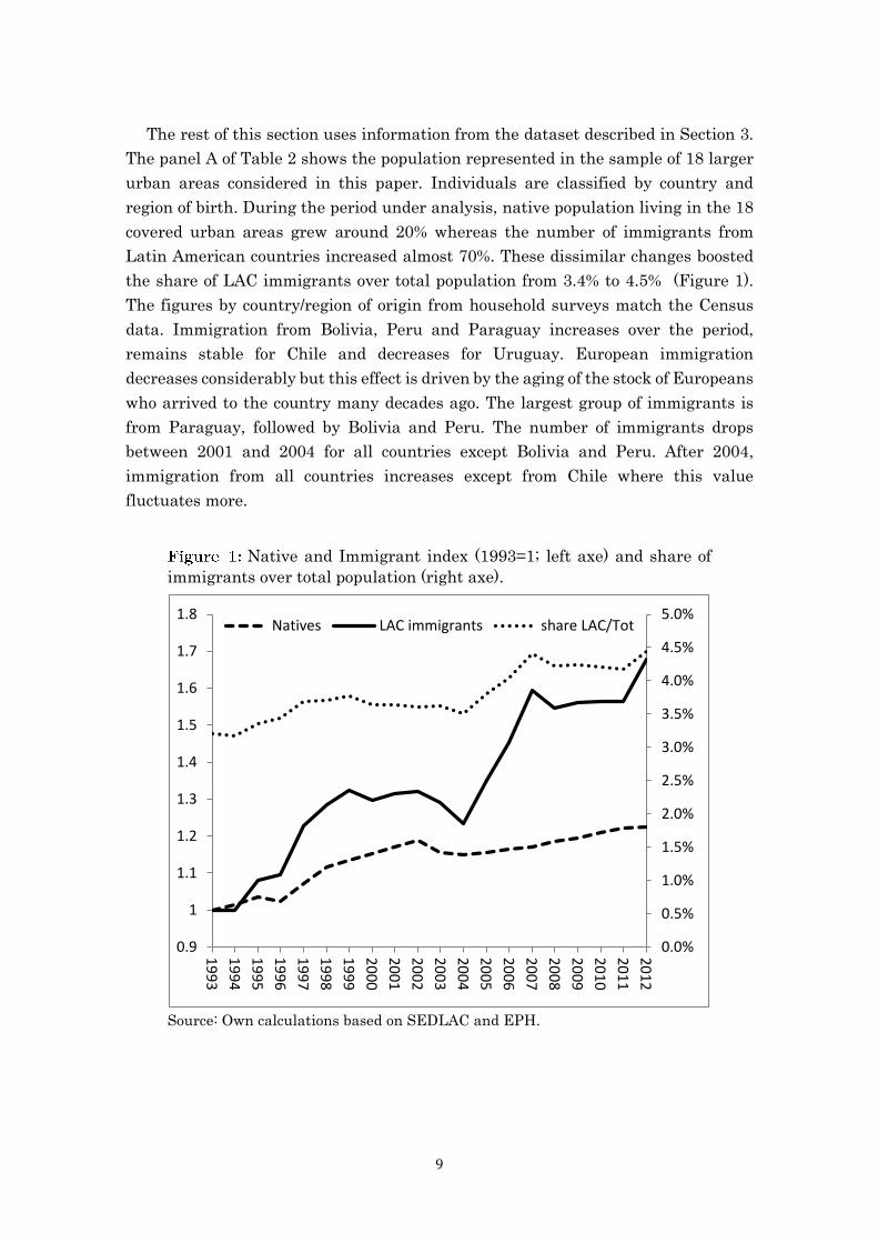
The rest of this section uses information from the dataset described in Section 3.

The panel A of Table 2 shows the population represented in the sample of 18 larger

urban areas considered in this paper. Individuals are classified by country and

region of birth. During the period under analysis, native population living in the 18

covered urban areas grew around 20% whereas the number of immigrants from

Latin American countries increased almost 70%. These dissimilar changes boosted

the share of LAC immigrants over total population from 3.4% to 4.5% (Figure 1).

The figures by country/region of origin from household surveys match the Census

data. Immigration from Bolivia, Peru and Paraguay increases over the period,

remains stable for Chile and decreases for Uruguay. European immigration

decreases considerably but this effect is driven by the aging of the stock of Europeans

who arrived to the country many decades ago. The largest group of immigrants is

from Paraguay, followed by Bolivia and Peru. The number of immigrants drops

between 2001 and 2004 for all countries except Bolivia and Peru. After 2004,

immigration from all countries increases except from Chile where this value

fluctuates more.

Native and Immigrant index (1993=1; left axe) and share of

immigrants over total population (right axe).

Source: Own calculations based on SEDLAC and EPH.

0.0%

0.5%

1.0%

1.5%

2.0%

2.5%

3.0%

3.5%

4.0%

4.5%

5.0%

0.9

1

1.1

1.2

1.3

1.4

1.5

1.6

1.7

1.8

19

93

19

94

19

95

19

96

19

97

19

98

19

99

20

00

20

01

20

02

20

03

20

04

20

05

20

06

20

07

20

08

20

09

20

10

20

11

20

12

Natives LAC immigrants share LAC/Tot

10

No. of individuals (thousands) represented in the sample (1993-2012).

The panel B of Table 2 shows the number of male workers with 18 to 65 years old

represented in the survey. This subsample constitutes the basis of the analysis in

this paper. Trends are similar than those discussed for total population. For this

subsample, in 2012 the largest number of immigrants is from Bolivia and Paraguay

YearNative

population

LAC

countriesBolivia Chile Paraguay Peru Uruguay Europe

1993 16,399 563.4 103.5 103.0 187.6 21.0 119.6 559.8 3.2%

1994 16,633 563.1 96.4 102.9 193.5 24.2 122.6 543.3 3.2%

1995 16,988 608.4 103.3 121.6 221.3 32.5 105.6 520.6 3.3%

1996 16,781 617.0 102.8 128.4 216.4 27.0 119.3 493.3 3.4%

1997 17,554 691.8 134.7 151.6 208.1 26.5 148.4 487.5 3.7%

1998 18,294 724.0 141.6 141.2 238.4 46.4 134.6 459.7 3.7%

1999 18,609 746.0 137.5 132.9 270.0 64.7 114.2 423.5 3.8%

2000 18,890 730.6 127.0 118.8 261.4 84.5 110.4 389.8 3.6%

2001 19,217 740.6 138.0 114.8 282.5 77.6 95.4 353.7 3.6%

2002 19,509 743.1 188.1 112.6 261.5 64.7 89.2 365.5 3.6%

2003 18,941 726.4 179.9 103.6 232.6 81.9 104.9 353.4 3.6%

2004 18,821 695.4 161.2 105.3 247.3 79.8 81.2 287.7 3.5%

2005 18,958 761.5 195.7 103.4 263.1 76.3 99.0 283.3 3.8%

2006 19,119 818.2 216.6 92.4 285.0 92.9 103.9 263.2 4.0%

2007 19,209 897.9 247.0 86.5 262.7 155.3 107.7 249.7 4.4%

2008 19,421 870.2 195.9 91.1 305.6 120.6 121.5 261.4 4.2%

2009 19,598 879.2 209.3 107.4 312.3 116.7 91.8 253.5 4.2%

2010 19,808 881.3 221.0 110.2 322.0 119.3 72.2 232.5 4.2%

2011 20,009 881.4 203.5 106.4 309.1 127.3 91.2 211.4 4.2%

2012 20,068 945.8 228.6 95.5 322.0 154.2 91.0 212.4 4.4%

1993 3,588 171.2 27.6 35.7 53.1 11.2 41.7 100.5 4.4%

1994 3,574 179.0 31.5 31.9 58.7 10.9 42.7 100.3 4.6%

1995 3,470 174.4 33.1 35.3 57.3 10.6 35.4 93.7 4.6%

1996 3,442 174.9 33.1 37.5 52.7 9.3 37.5 80.6 4.7%

1997 3,728 210.9 40.5 44.8 58.6 8.4 54.9 84.6 5.2%

1998 3,900 213.7 34.9 44.0 71.7 10.6 48.9 86.9 5.1%

1999 3,903 212.3 37.7 41.9 70.6 18.9 40.2 74.2 5.1%

2000 3,917 211.3 37.4 37.0 69.1 25.1 38.3 58.3 5.0%

2001 3,836 199.2 37.2 33.1 69.7 17.5 33.6 41.9 4.9%

2002 3,720 197.3 51.5 28.5 60.9 21.3 29.1 40.6 5.0%

2003 3,907 193.6 54.4 22.5 53.8 20.0 35.8 48.3 4.7%

2004 4,179 212.5 51.4 34.2 77.0 20.3 27.5 35.9 4.8%

2005 4,300 235.2 61.0 34.0 75.7 21.6 37.4 37.9 5.1%

2006 4,409 247.4 66.0 29.6 81.8 23.1 39.6 37.2 5.3%

2007 4,531 249.9 74.7 27.7 63.9 34.4 38.4 36.8 5.2%

2008 4,584 260.7 63.9 29.8 81.3 31.4 47.3 34.5 5.3%

2009 4,615 244.8 61.4 31.9 81.3 30.7 30.0 35.2 5.0%

2010 4,766 255.4 66.8 31.1 89.8 35.4 24.2 20.4 5.1%

2011 4,898 262.5 68.5 28.8 83.3 33.3 37.9 15.6 5.1%

2012 4,778 268.1 75.3 20.3 72.5 42.3 43.0 27.6 5.3%

Notes: 18 major cities represented in 1993 survey. Source: Own calculations using SEDLAC and EPH.

A- Whole

sample

Immigrants by country/region of origin Share

LAC/total

population

B- Sub-

sample

of Men

[18-65]

11

followed by immigrants from Uruguay and Peru. The percentage of Latin American

immigrants in this subsample rose from 4.4% to 5.3% over the period under analysis.

It is important to mention that these figures relies on household surveys data

which is subjected to some methodological issues and higher measurement error

than census data.9

I follow Borjas (2003) and restrict most of the analysis for the subsample of men

aged 18-65 who participate in the labour force, however, some specifications use

information about men not active in the labour market. I also exclude from

regressions (and estimations related to earnings) those individuals who report

themselves as self-employed or those working at family firms without a well-defined

salary. Following Card and Lemieux (2001) and Manacorda, Manning and

Wadsworth (2012), I pool different years of the survey. Conversely to those works, I

define the length of each period as 4 years (instead of 5) to be consistent with the

distinction between new arrived and established immigrants defined for the same

length.10 Consistently to the definition of periods, I categorize individuals in 12 age-

groups of 4 years each. This decision contrasts with Borjas (2003), Bratsberg et al.

(2012) and Ortega and Verdugo (2011) who use experience instead of age. As pointed

by Card and Lemieux (2001) using age has the advantage of comparing individuals

who attended the same education level at the same time and therefore were

subjected to the same influences regarding their education decisions. On the other

hand, only potential experience can be identified in the data. Since there is not an

obvious way of partitioning labour force into age/experience categories, I perform

some robustness exercises in order to detect if results are driven by this specific

partition.

SEDLAC database define 6 levels of education which are homogeneous across

years and countries. This is an important feature since questionnaires have

undergone some changes in the educational module during the 20 years covered by

this work. I group the 6 levels into 4 broader educational levels consistently with

previous literature11. The categories are defined as 1) Primary education or no formal

education; 2) High school dropouts; 3) High school graduates or college dropouts; 4)

9 For household surveys analysis, comparison between ratios and proportions is more reliable

than comparison between absolute values, particularly across years. 10 After the second semester of 2003 the survey only allows to identify whether the immigrant

arrived within 4 years before the survey or not. 11 It is also inconvenient that partition into 6 education levels implies a large number of cells

with zero immigrants and low number of natives.

12

Professionals or university graduates. These definitions are more suitable for

Argentina than definitions used in Borjas (2003) for the US since a higher share of

workers are concentrated in low educational levels.

In order to relate as much as possible earnings with productivity (demand side)

avoiding at the same time the indirect effect of changes in supply decisions through

working hours, wages are defined as the total weekly earnings from the main

occupation divided by the number of worked hours in that occupation during the

week before the survey. In some specifications I also report monthly earnings from

main occupation. An important caveat that should be considered is the comparison

of wages across periods. The official Consumer Price Index reported by the Instituto

Nacional de Estadisticas y Censos (INDEC) in Argentina has been severely criticized

and widely discredited during the last few years due to a recurrently

underestimation of the true inflation. This concern is particularly relevant for the

last period considered in this paper (see for example Cavallo, 2013). For this reason

I deflate wages in the period 2008-2012 using the average of the non-official CPIs

reported by different private consultants.12 For the rest of the years I use the official

CPI.13 I exclude from earnings estimations all the individuals with hourly incomes

above $45 and below $0.2 (at 2010 prices).

Individuals are classified as immigrants based on their country of birth

irrespective of the age of arrival or their parents’ citizenship. Immigrants are

considered as “established” if they arrived to the country at least four years before

the survey. I focus on immigration from Latin American countries and ignore the

reduction in the stock of Europeans. There are two reasons for this decision, first,

most of the European immigrants who participate in the labour force arrived to the

country as children and second, the stock decline of European immigrants is mainly

due to retirement of workers who arrived during the 50s. Table A2 in the Appendix

shows evidence supporting these arguments. The median age of male European

immigrants participating in the labour force was already high in 1993 (53 years old)

and increased over the last 20 years. The median age of arrival is below 12 in any

survey and around 6 in the last 5 years with available information. The median year

of arrival is 1952 in almost all the surveys14. These characteristics suggest that

established European immigrants are highly assimilated to the local labour market

12 Gasparini and Cruces (2010) uses a similar index to evaluate the effect of a Conditional

Cash Transfers program. 13 Note however that all the models discussed in this paper use time fixed effects and time

interactions which absorb any proportional difference affecting all wages in the same period.

Therefore, the under/over estimation of the true inflation does not change the results. 14 Similar calculations for LAC immigrants show that median age is around 40 years and

constant in all the period, median age at arrival over 20 years and median year of arrival

rapidly increased from 1973 to 1984 during the 10 years with available information.

13

in the considered period. Based on these facts, I do not distinguish between natives

and established Europeans in the basic specification;

Finally, following the standard assumption in the literature, the measure of

labour supply is the number of individuals participating in the labour force instead

of the size of the working population. This assumption ignores the non-trivial

relationship between unemployment and wages but restrict the measure of labour

supply to changes in labour participation and migration shocks.

Table 3 presents the share of LAC immigrants and the mean hourly wage of

native men aged 18-65 for age-education cells in all periods. For presentation

purposes, I group the age categories into 6 groups instead of 12 as in the rest of

analysis. There are some repeated patterns like the drop in wages during the crisis

period 2001-2004. Over the same period the share of immigrants seems to increase

in some cells like those aged 34-41. This effect can be partly explained by selective

emigration of high skilled natives during the crisis period. Beyond these figures,

there is a large heterogeneity across cells and time in migration shares.

Percentage of immigrants and mean hourly wage by education-age cell. 18

urban areas. Employed men 18-65

Education

level

Age

groupt=1 t=2 t=3 t=4 t=5 t=1 t=2 t=3 t=4 t=5

18-25 3.3 3.5 3.5 4.4 8.0 2.4 2.1 1.6 1.9 2.3

26-33 6.0 6.6 5.3 7.2 7.6 2.8 2.6 2.0 2.3 2.9

34-41 6.7 7.7 8.4 7.3 5.7 2.9 2.9 2.2 2.7 3.1

42-49 7.1 8.3 6.7 6.5 7.7 3.2 3.0 2.5 2.9 3.4

50-57 7.1 7.9 7.6 6.7 5.5 3.3 3.2 2.5 2.9 3.5

58-65 5.0 8.1 8.6 7.8 8.4 3.4 3.3 2.5 3.1 3.6

18-25 2.8 2.9 2.0 2.9 3.8 2.6 2.3 1.7 2.2 2.6

26-33 5.3 5.5 4.3 5.0 3.3 3.2 2.9 2.3 2.8 3.1

34-41 5.4 6.3 7.4 6.8 4.5 3.9 3.3 2.6 3.1 3.6

42-49 6.2 5.5 5.1 6.2 6.9 4.3 4.2 3.0 3.5 3.9

50-57 6.4 7.4 7.8 7.7 6.5 4.7 4.5 3.1 3.5 3.9

58-65 3.0 7.2 7.0 6.6 6.0 4.5 4.6 3.3 3.9 4.1

18-25 2.3 2.2 2.4 3.3 3.9 3.3 3.3 2.5 3.1 3.5

26-33 4.9 4.7 3.7 4.0 4.6 4.5 4.2 3.2 3.6 4.2

34-41 4.4 4.9 6.7 5.8 6.7 5.5 5.3 3.8 4.3 4.9

42-49 4.3 6.0 5.3 6.9 5.9 6.2 6.0 4.6 4.8 5.2

50-57 3.5 3.7 5.0 4.8 5.2 6.8 6.8 4.8 5.2 5.2

58-65 2.7 4.7 4.9 5.3 6.1 6.8 6.8 5.0 5.3 5.3

18-25 0.5 4.0 1.1 2.6 2.9 4.7 4.9 4.4 3.9 4.8

26-33 2.2 1.4 2.0 2.5 2.6 8.1 7.5 5.7 5.7 6.0

34-41 2.5 2.9 2.1 3.0 2.1 9.3 9.1 7.1 6.9 7.2

42-49 2.4 1.2 2.0 3.4 2.3 11.3 11.4 7.9 7.8 8.0

50-57 3.3 2.9 3.1 2.8 2.3 11.6 12.4 9.3 8.1 8.5

58-65 3.5 2.5 3.4 1.9 2.0 11.4 13.6 8.9 8.6 8.6

Notes: t=1: [1993-1996]; t=2: [1997-2000]; t=3: [2001-2004]; t=4: [2005-2008]; t=5: [2009-2012]. Wages are

measured in constant prices. Source: Own calculations using SEDLAC and EPH survey

High school

graduated or

university

dropouts

University-

professional

Share of LAC immigrants (%) Mean hourly wage of natives

Primary or

less

High school

droputs

14

Identification of the structural equations (7) and (9) relies on the validity of the

CES framework. Some cautionary notes about this point have been raised in recent

literature (see Aydemir and Borjas, 2011, Dustmann and Preston, 2011, Dustmann,

Frattini and Preston, 2012). Alternatively, a first approach to the effect of

immigration on wages without relying on further structural assumptions is the

estimation of the following reduced form wage equation proposed by Borjas (2003):

(10) log ( ) ( ) ( )ineat meat e a t e t a t a e ineat ineat

w P d d d d d d d d d X

where meat

P is the share of immigrant labour force on the total supply of workers with

education e, and experience a at time t. The variables , ,e a t

d d d are education,

experience and time fixed effects. Interactions capture education and experience

specific time trends as well as any possible interaction between education and

experience. Therefore, fixed effects and interactions absorb any effect on wages

produced by a shift in the total number of workers, changes in the skill or age

composition of the labour supply and any possible specific change in the age-

experience cells. Since the triple interaction a e t

d d d is omitted, identification is

achieved through changes in the immigrant composition of each experience-skill cell

across time. Under perfect substitution between natives and immigrants (i.e.

ct ct ctL N M for every cell c), equation (10) can be easily derived as a first order

approximation of the equilibrium market condition when the cell-specific labour

demand takes the (generic) form: log logct ct ctw L and the supply of native

workers at cell c respond to changes in wages according to

/ logct ct ct ct

N N w (see Borjas, 2003). The expression is derived as the

difference in wages relative to a counterfactual scenario of no immigration.

If the share of immigrants varies exogenously within cells, φ can be interpreted

as the causal (partial) effect of a shift in the supply of immigrants on the wage of

native workers. In this context, exogeneity means uncorrelation between the

migration inflow and any cell-specific shock. For instance, a potential violation of

exogeneity is produced when individuals migrate anticipating a future productivity

boom, since this confounds the change in wages produced by the increase in the

labour supply with the increase in the demand. Nevertheless, this bias is positive

and a negative value of φ should be interpreted as a lower bound. Similarly,

identification can be undermined if immigrants enter to cells where the demand is

simultaneously falling. When demand shocks are independent across countries, this

behaviour is a very unlikely prediction since immigrants should be attracted to

growing-demand sectors, nevertheless, if the demand in the same cell is falling faster

15

in the country of origin, this is an important concern. Related works have not been

able to solve this issue when dealing with non-experimental data15 but something

can be inferred by including (potentially endogenous) controls at demand level

within each cell (Bratsberg et al, 2011).

An additional caveat is the potential selectivity bias produced by non-random

dropping of native population from labour force when shifts in the supply reduce

wages below the reservation wage of marginal workers. Selectivity problem is

difficult to control even with panel data because Equation (10) is semi-saturated and

residual variation is usually very low. In the context of Argentinean labour market,

the non-random emigration of native population in reaction to falling wages is also

a potential source of endogeneity since it artificially increases the share of

immigrants when wages are relative low.

The Borjas’ setting (Eq. 10) has the additional problem that φ also accounts for

the increase in the share of immigrants due to changes in the size of native labour

force. On the top of that, its interpretation is not strongly connected with the

theoretical model discussed before. Indeed, it is possible that the size of some cells

grow over time due for example to a secular increase in the education of the native

population. If the inflow of immigrants is biased toward these growing cells, the

estimations of φ will be negatively biased. An alternative equation can be derived

from (7) keeping the assumption that immigrants and natives are perfect substitutes

within cells in the production function ( 1). Under this assumption, the wage

equation can be written as:

log log ( )log ( 1)log( )neat t et ea t et neat eat meat

w Y v L L L b L

Defining ( / )meat meat neat

R L L as the ratio of immigrants to natives within each cell

and using the fact that log(1 )x x for small x, it is straightforward to show that the

following approximation holds:

log log ( )log ( 1)log ( 1)neat t et ea t et neat eat meat

w Y v L L L b R

An estimable reduced form equivalent to the last equation is given by:

(11) log log ( ) ( ) ( )ineat meat neat e a t e t a t a e ineat

w R L d d d d d d d d d

15 Card (1991) estimation of the impact of the Mariel’s Boatlift event is a well-known example

of quasi-experimental variation of the immigrant labour supply. Other examples using quasi-

experimental variation of immigrants are Glitz (2012), De Silva et al. (2010), and Hunt (1992).

16

Obviously, the main concern when implementing (10) or (11) is the potential

endogeneity of neat

L , meat

R and meat

P . In the next sub-section, I discuss alternative IV

strategies to cope with the potential endogeneity of the immigrant share/ratio.

The reduced form version for the Borjas’ model with imperfect substitution

between immigrant groups is given by:

(12) 1

log ( ) ( ) ( )J

ineat j jmeat e a t j e t a t a e ineatj

w P d d d d d d d d d d

This simply corresponds to replacing the share/ratio of immigrants by similar

measures but disaggregated by country of origin. Note that the assumption that all

immigrants are perfect substitutes with natives independently of the country of

origin (and provide similar efficiency units) imposes the testable constraint

1 2 ... M in (12). Similarly, perfect substitution between immigrant groups

would imply that meat jmeatj

R R in equation (11) which is also a testable hypothesis.

In this work, I will focus on immigrants from Bolivia, Chile, Paraguay, Peru and

Uruguay since they account for most of immigration.

To see an example of why heterogeneity could be relevant, Tables A3 and A4 in

the appendix shows the distribution of high and low educated workers across

industries by country of origin. There are important differences in the cross-country

pattern. For example in the period 1993-1996 44% of the Bolivian low skilled

immigrants worked in the construction sector whereas only 12% of the low skilled

Peruvian immigrants worked in this sector. The differences in Tables A3 and A4 are

systematic for all countries and industries and also change over time. This suggests

that the impact of immigration can be heterogeneous across countries of origin.

Occupational differences could be strictly related with observed variables like

education and age. In such case, this effect does not translate into heterogeneous

impact within this model. However, Ortega and Verdugo (2011) find that

unobservable factors can simultaneously explain wage determination and the

occupational decisions of immigrants. Vela and Pattel (2007) also find that networks

play an important role in explaining this heterogeneity.

Identification of (10)-(12) requires that the changes in the measure of immigrant

penetration along time (and within each cell) are related only with exogenous shifts

of the relative labour supply. The key assumption is that all the changes within cells

of education-age groups are not induced by demand changes or correlated with cell-

specific shocks. As described in the previous sub-section, the most critical potential

deviation from this assumption is when the immigration-native composition changes

17

in response to rising wages due to a demand shift. Nevertheless, this bias is positive

and a negative value of the estimations should be interpreted as a lower bound.. The

strength of the semi-saturated specification is that it controls for any type of

endogeneity related with aggregated demand shifts even at the level of education or

age dimension. Naturally, there is still a chance that shocks are spread in a

heterogeneous way across cells leaving some endogenous component uncontrolled.

A natural way to cope with confounding demand factors is to include some proxy

control like the unemployment rate for native population. Although this proxy can

uncover some bias, it is endogenous and fails to capture the whole demand variation.

Consequently, a second IV strategy is proposed and discussed at the end of this

subsection.

A second identification issue is the endogeneity of the participation decision

among natives and already established immigrants. To control for this potential bias,

I follow the strategy proposed in Borjas (2003) and instrument the measures of

relative supply with similar measures but at population level, that is, including also

non-participant individuals. The intuition behind this instrument is that changes in

the population size only affect wages through the increase in the labour supply but

the size and the age-education composition of the population is fixed in the short run

for natives. Similarly, changes in the number of immigrants are connected with

changes in wages only through the labour market. Thus, the total number of

immigrants is assumed to be exogenous once we control for the size of the immigrant

labour force. A downside of this instrument is that it ignores the changes in the

population (native or immigrant) due to emigration, particularly when individuals

leave the country due to falling wages in their education-age cell. Comparing results

from equations (10) and (11) can uncover the potential negative bias due to native

emigration. The latter equation controls for the size of the native labour force and

therefore is less affected by native emigration. The return of immigrants to their

home countries in response to wage drops introduce a positive bias and therefore,

negative values of the coefficients in (10) or (11) should be interpreted as lower

bounds.

An additional concern is the lack of coverage of rural areas and small cities in the

sample. Internal migration can induce changes in the immigrant composition of the

labour force if native workers move into large cities in response to changes in labour

market conditions. I include the number of internal immigrants in some

specifications in order control for this source of endogeneity.

In order to isolate the supply variation from demand cell-specific shocks and other

confounding factors, I exploit available micro-data from other countries to build an

18

instrument which relates changes in the supply of immigrants with variations in the

economic conditions in their countries of origin.16

I pool different surveys from each country into 5 periods of 4 years length in the

same way described for the Argentinean dataset. Unfortunately, the set of years

available for each period varies from country to country as shown in Table 1.

Estimations for the first period (1993-1996) are based on fewer surveys than

estimations for the later periods.17

The first set of instruments is defined as:

(13) ,( 1),( 1)

1

1 Jj

eat e a tj

Z wJ

where ,( 1),( 1)

j

e a tw

is the hourly wage in country j in the period t-1 for the education-

age group (e,a-1). Note that the age group is also lagged to track the same cohort

over time. Wages are comparable and measured in 2005 USD-PPP prices. The

relevance of the instrument comes from the fact that negative shocks in the country

of origin increase the incentives to emigrate.18 To account for a possible non-linear

relationship between income in origin and migration I also include the squared

instrument (see for example Chiquiar and Hanson, 2005 and Grogger and Hanson,

2002, 2011).19

Using lagged variables instead of contemporaneous information has two

advantages. On the one hand, demand shocks can affect the wages of particular

education-age cells in all the countries at the same time (including Argentina) and

this could invalidate the instrument.20 On the other hand, migration is a costly

decision and do not react instantaneously to shocks in the country of origin.

As a robustness check, a second strategy uses the whole set of , ( 1), ( 1)je a tw as

instruments instead of the average across countries. This specification is more

flexible but in the presence of a weak first stage, the resulting bias increases with

16 Munshi (2003) uses a related strategy by instrumenting the number of Mexican

immigrants with the rainfall level in the home village. In this case, such type of instruments

is not useful because is perfectly correlated with the set of fixed effects and interactions. 17 In the case of Peru, data from the first period comes from Census without information

about incomes or worked hours and therefore I only use unemployment rates from this

country. 18 I avoid using also unemployment as instrument because it is less correlated with

immigration. The main reason is that unemployment is usually low for highly informal

markets and do not change significantly over time. 19 The first paper claims that propensity to migrate changes along the income distribution.

The other papers test immigrant selection under different specifications of the indirect utility

function. 20 Obviously, nothing preclude that some countries are affected by contagion but observations

are separated by lags of 4 years on average and this reduce the likelihood of such effect.

19

the number of instruments (Hahn and Hausman, 2002). In regressions with many

fixed effects and interactions like Equations (10) or (11), achieving a strong first

stage is commonly difficult.

Finally, I consider an instrument that exploits all the information available for

each country of birth. Card (2001) uses the lagged regional distribution of

immigrants to predict the actual distribution at cell level and uses this prediction as

a valid instrument. I follow a related strategy and predict the cell-distribution of

immigrants from each country using all the available information one period lagged

(excluding Argentina). 21 For example, I predict the number of immigrants from

Bolivia, with primary education aged 30-33 in period t=2, using information on

wages and unemployment from the 6 countries of origin in t=1 for individuals with

the same education but aged 26-29. 22 The variables I use to build this set of

instruments are the unemployment rate, the log hourly wage, the log monthly wage

and the average number of worked hours. 23

An important point is that, as previously discussed for the baseline specification,

validity of the instruments is not affected by aggregated shocks, education-specific

shocks, age-specific shocks or any persistent process involving them because the set

of fixed effect and interactions is also included in the first stage. As I show in the

results section, this convenient feature also creates some concerns about the power

of the first stage because after controlling for all the set of interactions, the residual

variation of the instrument can be weakly correlated with the immigration

explanatory variable.24

Borjas, Freeman and Katz (1997) and Borjas (2003) raised an important question

about the validity of previous studies that used geographical variation in

immigration flows as identification strategy. 25 According to this critique, if cities

within a country operate as open economies, supply shocks will be spread across

them and wages will tend to be equalized. If this hypothesis is true, the magnitude

of the impact estimated using cities or regions as unit of comparison across time,

should be biased toward zero. Additionally, if immigrants can decide the settlement

21 Using the whole set of lagged measures directly as instruments would account for 21

instruments, leading to a large small-sample bias as discussed in Hahn and Hausman (2002). 22 I include information from all countries to account for cross-country effects of shocks. For

example, a positive shock in Peru can reduce immigration from Bolivia to Argentina. 23 I use worked hours since informal work is extremely high in some countries and

unemployment is not an accurate measure of economic conditions. In most cases,

unemployment rate is very low since many workers perform low remunerated tasks during

a few hours a week. 24 This trade-off between exogeneity of the instrument and power of the first stage is one of

the points discussed in Stock, Wright and Yogo (2002). 25 For example Altonji and Card (1991), Card (1990), LaLonde and Topel (1991).

20

place, it is likely that cities or regions with booming wages will attract a higher share

of immigrants inducing a positive correlation between wages and immigration.26 I

explore this setting by replicating some of the previous results at the level of city-

education-age cell. The stratification is based on the 18 urban areas described in

Table A1 in the appendix.

Reduced forms (10) and (11) cannot be interpreted as the total impact of

immigration on wages. For instance, the interaction terms capture the indirect effect

of immigration on wages trough the change in cell’s total employment.

Complementarities among education groups or age/experience groups could even

change the sign of the impact if we also consider cross-cell effects. Therefore, φ

should be interpreted as a partial direct derivative which only captures the average

impact of immigration among similar workers. Moreover, this effect is assumed to

be homogenous across cells, which is a strong assumption. Additionally, both

specifications assume that immigrants and natives are perfect substitutes within

each cell. The structural parameters of the model can reveal more information about

the total effect of immigration and potential imperfect substitution across groups.

For the model with imperfect substitution by country of origin, the structural

parameters can be estimated extending the procedure proposed in Manacorda,

Manning and Wadsworth (2012) for the case of imperfect substitution between

immigrants. This extension is straightforward but beyond the scope of this paper.

Table 4 reports OLS and 2SLS estimates for the reduced form proposed by Borjas

(Equation 10 - Panel A) and the first order approximation of the CES model

(Equation 11 - Panel B). 2SLS uses population measures as instruments for labour

force variables. Following the discussion in Section 5, all the results presented

throughout this paper are estimated using both equations.

Dependant variables are the average log hourly wages and the average log

monthly earnings calculated at each education-age-time cell for men aged 18-65.

standard errors are clustered at education-age level to allow for autocorrelation

within cells over time. Additionally, all the regressions are weighted by the sample

size of each cell at every period.

26 However, Card and DiNardo (2000) find little evidence of such effect.

21

OLS results indicate that immigration has a significant (partial) negative effect

on wages under any specification. The point estimates are close to -1 for the first

specification and around -0.8 for the second specification. The magnitude of this

effect is higher than the effects find by Borjas (2003) for the US.27 The elasticity of

wage to immigration can be calculated as 2log / / (1 )eat eat eatw R R in the first model

and simply φ in the second model. Over the whole period, the average ratio of LAC

immigrants to native population is 0.053. This implies that elasticity in the first

specification is close to -0.9 and around -0.8 in the second model. It is not surprising

that the first specification results in a higher impact because it fails to control for

changes in the share of immigrants induced by changes in the absolute number of

natives. This is a particular concern for the case of Argentina because native’s

emigration rate is high for periods of low economic activity.

Impact of immigration on wages. Reduced form specifications

The second OLS specification in Table 4 includes the native’s unemployment rate

as a proxy control for demand side shocks. This is an endogenous variable but

coefficients remain very stable after its inclusion. The sign of the unemployment

coefficient is negative as expected although non-significant.

27 Borjas (2003) finds coefficients between -0.54 and -0.63 for Log weekly earnings and

between -0.72 and -1.23 for annual earnings. Estimated elasticities of earnings to

immigration are between -0.4 and -0.9.

A. Baseline model (eq. 10)

Share of LAC immigrants -1.084** -1.070** -1.106** -1.091** -0.865*** -0.808** -0.882*** -0.824**

(0.436) (0.496) (0.442) (0.508) (0.331) (0.368) (0.334) (0.375)

Native's unemployment rate -0.126 -0.122 -0.111 -0.104

(0.227) (0.288) (0.167) (0.211)

B. Model 2 (eq. 11)

Ratio LAC immigrants/Natives -0.780** -0.786** -0.797** -0.803** -0.631** -0.609** -0.646** -0.623**

(0.325) (0.385) (0.330) (0.392) (0.256) (0.293) (0.259) (0.297)

Log size of native labour force 0.115*** 0.100** 0.115*** 0.099** 0.094*** 0.070* 0.092*** 0.069*

(0.038) (0.047) (0.038) (0.046) (0.028) (0.036) (0.028) (0.035)

Native's unemployment rate -0.107 -0.104 -0.096 -0.092

(0.207) (0.271) (0.153) (0.200)

Log hrly

wage

Log mthly

wage

Notes: Robust standard errors are adjusted for clustering within education-age cell. All the calculations are based

on 240 observations. Regressions are weighted by the sample size of each education-age-time cell. The 2SLS

estimations instrument the share of immigrants participating in the labour force with the share of immigrants in the

population in the same education-age-time cell, lagged by period and cohort (see section 5 for details). Similarly,

the ratio of immigrants and the Log size of native labour force are instrumented with the corresponding population

measures (see text for details). The sample consists of men aged 18-65. Source: Own calculations using SEDLAC and

EPH survey.

Additional controls: time fixed effects, education fixed effects, age fixed effects, education-age interactions,

education-time interactions, age-time interactions

Log hrly

wage

Log mthly

wage

Log hrly

wage

Log mthly

wage

Log hrly

wage

Log mthly

wage

OLS 2SLS

Baseline

controls

Include demand

control

Baseline

controls

Include demand

control

22

The second group of columns in Table 4 presents the Two Stage Least Squares

estimations using population measures as instruments for labour force variables.28

As extensively discussed in section 5, this intends to control for the potential

endogeneity in the decision of participating into the labour force. Point estimates are

slightly smaller in absolute value, indicating that there is some positive correlation

between wages and the participation decision of native population.29 This hypothesis

is also consistent with the reduction in the coefficient estimated for the log size of

native labour force in Panel A. A positive value of this coefficient (after

instrumenting with population size) can be explained by different effects, first, a

strong emigration response of natives to wage drops, second, higher wages can

attract internal migrants from rural areas or small cities and finally, in terms of the

theoretical model discussed in Section 2, a low elasticity of substitution across ages

or education groups.

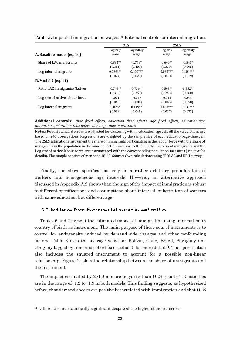
In order to explore the potential bias due to internal mobility, Table 5 shows OLS

and 2SLS results when the number of internal immigrants in the cell is included as

regressor. Internal immigrants are defined as those individuals who do not live in

their birth province.30 This variable is highly correlated with immigration from rural

areas or small cities not covered in the survey. The evidence suggests that internal

mobility could explain the positive estimated coefficient of the log size of native

labour force. Indeed, the estimates for this variable become close to zero or negative

after controlling for internal migration. Moreover, the coefficient of the number of

internal migrants is positive. Since it is very unlikely that internal migrants are not

perfect substitutes with other natives, this positive sign can be caused by the

endogenous effect of wages on internal mobility. Under both models, the coefficients

of the LAC immigration variable remain significant. In the first specification point

estimates drop around 20% in absolute value and in the second specification they

remain almost unchanged. The implied wage elasticities are around -0.7 for OLS and

in the range of -0.5 to -0.6 for 2SLS estimations. These values are in line with Borjas’

estimations for the US.

28 First stage is not reported since by construction instruments are highly correlated with

explanatory variables and F statistics above 200. 29 Higher wages would increase the participation rate of natives (relative to immigrants) and

this would artificially reduce the share of immigrants introducing a negative bias in the

estimation. 30 I do not use migration at municipal level since some urban areas like Great Buenos Aires

are comprised by many municipalities.

23

Impact of immigration on wages. Additional controls for internal migration.

Finally, the above specifications rely on a rather arbitrary pre-allocation of

workers into homogeneous age intervals. However, an alternative approach

discussed in Appendix A.2 shows than the sign of the impact of immigration is robust

to different specifications and assumptions about intra-cell substitution of workers

with same education but different age.

Tables 6 and 7 present the estimated impact of immigration using information in

country of birth as instrument. The main purpose of these sets of instruments is to

control for endogeneity induced by demand side changes and other confounding

factors. Table 6 uses the average wage for Bolivia, Chile, Brazil, Paraguay and

Uruguay lagged by time and cohort (see section 5 for more details). The specification

also includes the squared instrument to account for a possible non-linear

relationship. Figure 2, plots the relationship between the share of immigrants and

the instrument.

The impact estimated by 2SLS is more negative than OLS results.31 Elasticities

are in the range of -1.2 to -1.9 in both models. This finding suggests, as hypothesized

before, that demand shocks are positively correlated with immigration and that OLS

31 Differences are statistically significant despite of the higher standard errors.


Share of LAC immigrants -0.834** -0.778* -0.640** -0.545*

(0.361) (0.403) (0.279) (0.295)

Log internal migrants 0.086*** 0.100*** 0.089*** 0.104***

(0.024) (0.027) (0.018) (0.019)

B. Model 2 (eq. 11)

Ratio LAC immigrants/Natives -0.748** -0.736** -0.593** -0.552**

(0.312) (0.353) (0.243) (0.260)

Log size of native labour force 0.021 -0.047 -0.011 -0.088

(0.066) (0.080) (0.045) (0.058)

Log internal migrants 0.076* 0.119** 0.093*** 0.139***

(0.039) (0.045) (0.027) (0.033)

Notes: Robust standard errors are adjusted for clustering within education-age cell. All the calculations are

based on 240 observations. Regressions are weighted by the sample size of each education-age-time cell.

The 2SLS estimations instrument the share of immigrants participating in the labour force with the share of

immigrants in the population in the same education-age-time cell. Similarly, the ratio of immigrants and the

Log size of native labour force are instrumented with the corresponding population measures (see text for

details). The sample consists of men aged 18-65. Source: Own calculations using SEDLAC and EPH survey.

Log mthly

wage

Additional controls: time fixed effects, education fixed effects, age fixed effects, education-age

interactions, education-time interactions, age-time interactions

OLS 2SLSLog hrly

wage

Log mthly

wage

Log hrly

wage

24

results are positively biased. Estimations are not significant after including the

internal migration control but the coefficients are still negative and high.

Impact of immigration on wages. Instruments based on the average wage

in immigrants’ country of origin lagged by period and cohort.

The 2SLS results also imply either a very high substitution across education and

age groups or a high degree of substitution between natives and immigrants. An

interesting result is that the coefficient of the log size of the native labour force

becomes negative in contrast with the baseline regressions. A drawback of these

estimations is that the first stage is not very strong with F-statistics between 3 and

4 (significant in all cases). This is not surprising because the first stage includes a

huge number of fixed effects and interactions that remove most of the variation in

the instruments. As a result, residual variation is only weakly correlated with the

immigration measures for each specific cell. Additionally, regressions exclude the


Share of LAC immigrants -2.157** -1.942* -2.177** -1.845* -1.371 -1.324

(0.856) (1.081) (0.890) (1.116) (0.963) (1.441)

Native's unemployment rate -0.027 0.136

(0.199) (0.265)

Log internal migrants 0.052 0.064

(0.035) (0.049)

F excluded instruments 1 3.755 3.755 3.998 3.998 4.058 4.058

B. Model 2 (eq. 11)

Ratio LAC immigrants/Natives -1.631* -1.584 -1.648* -1.447 -1.364 -1.268

(0.865) (1.181) (0.946) (1.279) (0.869) (1.275)

Log size of native labour force 0.013 -0.002 0.012 0.011 -0.047 -0.095

(0.058) (0.075) (0.063) (0.080) (0.062) (0.078)


(0.210) (0.282)

Log internal migrants 0.067* 0.101**

(0.039) (0.051)



Notes: Robust standard errors are adjusted for clustering within education-age cell. All the calculations

are based on 173 observations. Regressions are weighted by the sample size of each education-age-time

cell. 2SLS : Instrument for the share/ratio of immigrants is the average lagged hourly-wage and its

square fo each education-age cell among the five most popular countries of origin among immigrants

(see Section 5 in text for details). Log size of native labour force instrumented with the population size

of the corresponding cell. The sample consists of men aged 18-65. Source: Own calculations using

SEDLAC and EPH survey.

2SLS



Baseline

controls

Include demand

control

Include internal

migration control

Log hrly

wage

Log mthly

wage

Log hrly

wage

Log mthly

wage

Log hrly

wage

Log mthly

wage

25

first period (because of lagging) and therefore precision decreases considerably.

Figure 3 plots the relationship between the share of immigrants and the first stage

prediction after removing the effect of other regressors like fixed effects and

interactions.

Share of immigrants and excluded instrument

Note: Each observation corresponds to a different education-age cell

at a particular period.

First Stage

Note: Both variables are residuals from a regression on the set of

fixed effects and interactions by age, education and time.

26

Table 7 shows the 2SLS results when the instruments are included in the first

stage disaggregated by country of origin. Estimations become even more negative

than before and remain significant in all cases. Implied elasticities are clustered

around -1.7 and -2.1. The power of the first stage does not improve relative to Table

6 and F statistics are between 2.8 and 3.4.

Impact of immigration on wages. Alternative set of Instruments

disaggregated by country of origin.

Table A5 in the Appendix presents the estimations for the alternative set of

instruments discussed in section 5. The first group of columns uses the predicted

distribution of immigrants from lagged cell-specific information from Bolivia, Chile,

Brazil, Paraguay, Peru and Uruguay (See Section 5 for more details). The F statistics

of the first stage rise above 4 after including the demand controls. Point estimates


Share of LAC immigrants -2.449*** -2.450*** -2.438*** -2.411*** -2.031** -1.994*

(0.805) (0.803) (0.834) (0.822) (1.020) (1.098)


(0.212) (0.280)

Log internal migrants 0.035 0.046

(0.036) (0.044)


B. Model 2 (eq. 11)

Ratio LAC immigrants/Natives -2.064** -2.247** -2.032** -2.162** -1.871** -1.911*

(0.873) (0.972) (0.957) (1.027) (0.893) (1.011)

Log size of native labour force -0.004 -0.034 -0.004 -0.026 -0.058 -0.117*

(0.057) (0.062) (0.064) (0.066) (0.062) (0.067)


(0.234) (0.300)

Log internal migrants 0.056 0.091*

(0.039) (0.051)



Notes: Robust standard errors are adjusted for clustering within education-age cell. All the calculations

are based on 173 observations. Regressions are weighted by the sample size of each education-age-time

cell. 2SLS : Instrument for the share/ratio of immigrants is the lagged hourly-wage and its square fo

each education-age cell in the five most popular countries of origin among LAC immigrants. The first

stage includes instruments dissagregated by country of origin of the immigrants (see Section 5 for

details). Log size of native labour force instrumented with the population size of the corresponding

cell. The sample consists of men aged 18-65. Source: Own calculations using SEDLAC and EPH survey.

2SLS

Baseline

controls

Include demand

control

Include internal

migration control



Log hrly

wage

Log mthly

wage

Log hrly

wage

Log mthly

wage

Log hrly

wage

Log mthly

wage

27

and standard errors are also higher. The weak instrument problem is neither

rejected in this case.

The results of the following sub-section indicates that instrumental variables

estimations should be interpreted with caution, but overall, the evidence from

different IV strategies suggests that demand shocks are positively correlated with

immigration flows and in this sense, the negative impact identified by OLS is a lower

bound for the true impact. For instance, Ortega and Verdugo (2011) estimate a bias

in the same direction.

As mentioned before, the weakness of the first stage is also the price of a stronger

exclusion restriction. The presence of a large list of fixed effects and interactions in

the first stage eliminates from the instrument the influence of any simultaneous

shock affecting all countries in the region, contagion processes and common trends

in wages. This is true even for shocks occurring within education or age groups.

In order to provide additional evidence about the relevance of the proposed

instruments, Table 8 summarizes alternative IV estimators. This strategy to cope

with potential weak instruments follows the discussion in Stock, Wright and Yogo

(2002), and Stock and Yogo (2002). The alternative estimators are the Limited

Information Maximum Likelihood estimator (LIML) and Jackknife IV estimation

(JIVE) proposed in Angrist, Imbens and Krueger (1999).32 The sets of instruments

presented are the same than those in Tables 2a and 2b. Differences between 2SLS

and LIML estimations usually indicate the presence of a bias due to weak

instruments since LIML is approximately median unbiased (Angrist and Pischke,

2008).33 In this case, LIML estimations are close to 2SLS results for the first set of

instruments (based on the average lagged wage in other countries) but not close for

the second set of instruments (which includes lagged wages disaggregated also at

country level). This result could be driven by the fact that 2SLS bias increases with

the number of excluded (weak) instruments and the second set of instruments is

large.

JIVE is usually described as an estimator with superior small sample properties

than 2SLS in the presence of weak instruments34. One of the sources of 2SLS bias is

the correlation between the error terms of the two stages for the same observation

ith. The JIVE procedure eliminates this correlation by excluding the observation ith

when predicting the fitted value of the endogenous regressor from the first stage. In

32 An alternative JIVE estimator is discussed in Blomquist and Dahlberg (1999). 33 2SLS is biased toward OLS in the presence of weak instruments. 34 Nevertheless, there is recent debate about this point that can be followed in Davidson and

MacKinnon (2006) and Ackerberg and Devereux (2006).

28

this case, JIVE estimations are lower than 2SLS and close to OLS results for both

set of instruments.35

Evidence from the alternative estimators do not allow to safely conclude that the

estimated impact of immigration is as high as 2SLS and LIML suggests, but in all

cases the point estimates remains significant and negative. Naturally, the exclusion

restriction relies on the assumption that fixed effects and interactions remove any

source of simultaneity in wage determination across countries. Without a

randomized variation in the amount of immigrants it cannot be ensured that this

assumption holds, but as discussed in previous sections, the direction of the bias

seems to operate toward zero. The results from different IV strategies do not

contradict this hypothesis.

Alternative IV estimators. Limited Information Maximum Likelihood

(LIML) and Jackknife IV estimation (JIVE)

Table 9 shows the impact of immigration when the total share of immigrants is

disaggregated by country of origin (Equation 12). In all cases other than Uruguay,

the estimated impact is negative but significant only for Bolivia and Peru.36 In most

cases, the hypothesis of homogenous impact by origin is rejected by the Wald test.

Further research is needed to understand this pattern. Particularly, the positive

impact of immigrants from Uruguay could be explained by two different effects. First,

35 A note of caution should be made since the JIVE procedure does not allow for clustering

standard errors and only heteroskedastic-robust standard errors are reported. 36 The OLS estimated coefficient for Chile is also significant when the hourly wage is the

dependant variable.

LIML JIVE LIML JIVE LIML JIVE LIML JIVE

Share (Ratio) of

LAC immigrants-2.516** -0.765** -2.211** -0.692** -4.521** -1.069** -3.595** -0.954**

(1.137) (0.340) (0.948) (0.299) (2.180) (0.537) (1.697) (0.463)



Notes: Robust standard errors are adjusted for clustering within education-age cell in the LIML and

adjusted for heteroskedasticity in the JIVE. All the calculations are based on 173 observations. The sample

consists of men aged 18-65. IV 1: Instrument for the share/ratio of immigrants is the average lagged

hourly-wage and its square fo each education-age cell among the five most popular countries of origin

among immigrants (see text for details). IV 2: Instrument for the share/ratio of immigrants is the lagged

hourly-wage and its square for each education-age cell in the five most popular countries of origin among

immigrants (see text for details). Baseline model uses the share of immigrants from LAC countries to

measure the impact of immigration. Model 2 is based on equation 11 in text and uses the Ratio of

imigrants to natives along with the size of the native labour supply. Source: Own calculations using

SEDLAC and EPH survey.

IV 1 IV 2

Baseline model Model 2 Baseline model Model 2

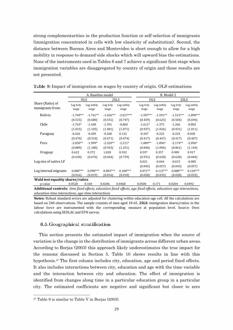
29

strong complementarities in the production function or self-selection of immigrants

(immigration concentrated in cells with low elasticity of substitution). Second, the

distance between Buenos Aires and Montevideo is short enough to allow for a high

mobility in response to demand-side shocks which will upward bias the estimations.

None of the instruments used in Tables 6 and 7 achieve a significant first stage when

immigration variables are disaggregated by country of origin and those results are

not presented.

Impact of immigration on wages by country of origin. OLS estimations

This section presents the estimated impact of immigration when the source of

variation is the change in the distribution of immigrants across different urban areas.

According to Borjas (2003) this approach likely underestimates the true impact for

the reasons discussed in Section 5. Table 10 shows results in line with this

hypothesis.37 The first column includes city, education, age and period fixed effects.

It also includes interactions between city, education and age with the time variable

and the interaction between city and education. The effect of immigration is

identified from changes along time in a particular education group in a particular

city. The estimated coefficients are negative and significant but closer to zero

37 Table 9 is similar to Table V in Borjas (2003).

Bolivia -1.749*** -1.741** -1.656*** -2.017*** -1.597*** -1.591** -1.515*** -1.890***

(0.515) (0.680) (0.551) (0.747) (0.459) (0.625) (0.504) (0.694)

Chile -1.743* -1.448 -1.391 -0.860 -1.611* -1.375 -1.266 -0.802

(1.015) (1.105) (1.001) (1.071) (0.937) (1.026) (0.931) (1.011)

Paraguay -0.426 -0.209 -0.260 0.133 -0.347 -0.222 -0.224 0.028

(0.470) (0.510) (0.471) (0.474) (0.417) (0.447) (0.417) (0.407)

Peru -2.050** -1.999* -2.320** -2.211* -1.889** -1.896* -2.174** -2.096*

(0.889) (1.180) (0.923) (1.251) (0.840) (1.096) (0.861) (1.144)

Uruguay 0.622 0.372 1.028 0.932 0.597 0.357 0.989 0.917

(0.630) (0.676) (0.664) (0.739) (0.591) (0.628) (0.620) (0.684)

Log size of native LF 0.021 -0.044 -0.015 -0.085

(0.045) (0.057) (0.043) (0.057)

Log internal migrants 0.080*** 0.098*** 0.083*** 0.100*** 0.071** 0.115*** 0.088*** 0.134***

(0.016) (0.019) (0.016) (0.018) (0.028) (0.033) (0.028) (0.033)

Wald test equality shares/ratiosp-value 0.0520 0.160 0.0206 0.0468 0.0500 0.171 0.0204 0.0492

B. Model 2

Share (Ratio) of

immigrants from:

OLS 2SLS OLS 2SLS

Log hrly

wage

Log mthly

wage

Log hrly

wage

Log mthly

wage

A. Baseline model

Notes: Robust standard errors are adjusted for clustering within education-age cell. All the calculations are

based on 240 observations. The sample consists of men aged 18-65. 2SLS: immigration shares/ratios in the

labour force are instrumented with the corresponding measure at population level. Source: Own

calculations using SEDLAC and EPH survey.

Additional controls: time fixed effects, education fixed effects, age fixed effects, education-age interactions,

education-time interactions, age-time interactions

Log hrly

wage

Log mthly

wage

Log hrly

wage

Log mthly

wage

30

compared with previous results. Borjas (2003) and Ortega and Verdugo (2011) also

find lower effects from regional stratification.

The second column adds to the previous specification the three-way interaction

between city, education and age. In this case, identification comes from comparing

the same education-age-city cell in different periods. The coefficient from Borjas’

model is still negative and significant but in the second specification it is not.

Impact of immigration on wages using geographical stratification. OLS

estimations

The third and fourth columns add the others three-way interactions allowing for

time effects to vary across education-age, city-age, and city-education cells. Only the

first specification remains significant in the third column and the last column’s

results are close to zero for both models. Naturally, these findings do not imply that

immigration effect dilutes as it is spread across cities. Indeed, this pattern can be

driven by a large attenuation bias resulting from the high level of data

disaggregation and the small residual variability after controlling for a larger set of

interactions and fixed effects (see the discussion in Borjas, 2003).

This paper evaluates the effects of cross-border immigration on the wages of

Argentinean native workers over the period 1993-2012. As discussed in Section 1,

Share of LAC immigrants -0.110** -0.169** -0.139* 0.029

(0.054) (0.080) (0.079) (0.100)

Ratio LAC immigrants/Natives -0.046** -0.032 -0.013 0.010

(0.023) (0.040) (0.039) (0.056)

Time, Age, Education, City YES YES YES YES YES YES YES YES

Time × Age , Time × Education,

Time × City, Education × CityYES YES YES YES YES YES YES YES

Education × Age × City NO YES YES YES NO YES YES YES

Education × Age × Time NO NO YES YES NO NO YES YES

Education × City × Time,

Age × City × TimeNO NO NO YES NO NO NO YES

Notes: Dependant variable: Log hourly wage. Robust standard errors are adjusted for clustering within

education-age cell. All the calculations are based on 4013 observations. The sample consists of men aged 18-

65. Additional controls: Log-size of internal immigration in both models and Log size of native labour force

in the second model. Regressions are weighted by the population size of the cell. Source: Own calculations

using SEDLAC and EPH survey.

(1) (2) (3) (4) (1)

A. Baseline model B. Model 2

(2) (3) (4)

31

this is an important South-South corridor that has not received much attention in

the literature.

The main source of data for this paper is the Socioeconomic Database for Latin

America and the Caribbean (SEDLAC). Other sources of information include the

first semester round of the Argentinean EPH and the 1993 IPUMS Census Data for

Peru. All the variables are harmonized following the SEDLAC methodology.

The empirical setting follows a recent literature based on the “national approach”

proposed in Borjas (2003) which identify the labour supply variation with changes

in the size of predetermined skill groups, usually experience-age categories.

Alternatively to Borjas’ setting, I also estimate reduced form that can be obtained as

a log-linear approximation of the demand equation from the nested CES framework

proposed in Ottaviano and Peri (2012) or Manacorda, Manning and Wadsworth

(2012) under the assumption of perfect substitution between immigrants and natives.

Results from this methodology should be interpreted as a partial equilibrium effect

of immigration since cross-skills effects are captured by a large set of fixed effects

and interactions.

The paper also contrasts the baseline results with IV estimations from a set of

instruments based on labour market conditions in immigrants’ countries. An

alternative specification also explores the hypothesis of heterogeneous impact by

country of origin of immigrants.

OLS results show a significant negative impact of immigration with wage

elasticities in a range slightly above the estimated by Borjas (2003) for the US,

although controlling for internal migration results in similar wage elasticities. These

results are robust to different specifications and do not change when proxy-demand

controls are included. Although the literature agrees that OLS can be biased toward

zero, there are two potential confounders that need to be considered in this case. The

first one is emigration of native population in response to lower wages and the second

is internal migration from rural areas toward large cities. Estimations remain

significative after controlling for internal immigration rates although there is

evidence of some negative bias. Controlling for proxies of these factors reduces the

estimated impact but do not eliminate its significance.

IV estimations suggest that OLS results are a lower bound for the (partial) causal

effect of immigration as assumed by Borjas (2003). This implies that if there are

some confounder demand factors, they bias the results toward zero. IV results should

be interpreted with caution, the main drawback is a significant first stage but not

strong enough to reject a bias driven by a weak instrument problem. However, under

alternative estimators like LIML and JIVE, the sign of the estimated impact remains

negative.

32

The hypothesis of heterogeneous effect of immigration by country of origin cannot

be rejected in a reduced form. Nevertheless, results are rather imprecise due to high

measurement error and further research is needed to make additional inference

about the size of the impact. Particularly, estimation of the structural parameters of

the model would reveal more information about this effect.

Finally, when the supply shock is also identified from variations of immigration

at geographical level, the estimated impact is lower.

Ackerberg, D. and Devereux P. (2006) "Comment on 'The case against JIVE" Journal of

Applied Econometrics, John Wiley & Sons, Ltd., vol. 21(6), pages 835-838.

Altonji, J. and Card, D. (1991) “The Effects of Immigration on the Labor Market Outcomesof

Less-Skilled Natives,” in John Abowd and Richard B. Freeman, eds., Immigration, Trade

and Labor, University of Chicago Press 1991.

Angrist, J. D., Imbens G. and Krueger A. (1999) “Jackknife instrumental variables

estimation”. Journal of Applied Econometrics 14: 57-67.

Angrist, J. and Pischke, J (2008) “Mostly Harmless Econometrics: An. Empiricist's

Companion” Princeton, NJ: Princeton University Press.

Aydemir, A. and Borjas, G. (2011) "Attenuation Bias in Measuring the Wage Impact of

Immigration," Journal of Labor Economics, University of Chicago Press, vol. 29(1), 69-113,

01.

Blomquist, S. and Dahlberg, M. (1999) “Small sample properties of LIML and jackknife IV

estimators: Experiments with weak instruments,” Journal of Applied Econometrics 14:

69-88.

Borjas, G. (1987) "Self-Selection and the Earnings of Immigrants," American Economic

Review, American Economic Association, vol. 77(4), pages 531-53, September.

Borjas, G. (2003) “The labor demand curve is downward sloping: reexamining the impact of

immigration on the labor market,” The Quarterly Journal of Economics 118:1335-1374

Borjas, G., Freeman, R. and Katz, L. (1997) “How Much Do Immigration and Trade Affect

Labor Market Outcomes?,” Brookings Papers on Economic Activity, (1), 1–90.

Bratsberg, B., Raaum, O., Røed, M. and Schøne, P. (2010) "Immigration Wage Impacts by

Origin," Norface Discussion Paper Series 2010-2, Norface Research Programme on

Migration, Department of Economics, University College London.

Card, D. (1990) “The Impact of the Mariel Boatlift on the Miami Labor Market,” Industrial

and Labor Relations Review, 1990, 43 (2), 245–257.

Card, D. (2001) “Immigrant Inflows, Native Outflows, and the Local Market Impacts of

Higher Immigration,” Journal of Labor Economics, 19 (1), 22–64.

Card, D, and DiNardo, J. (2000) “Do Immigrant Inflows Lead to Native Outflows?,” The

American Economic Review, American Economic Association , 90 (2), 360–367.

Card, D. and Lemieux, T. (2001) "Can Falling Supply Explain The Rising Return To College

For Younger Men? A Cohort-Based Analysis," The Quarterly Journal of Economics, MIT

Press, vol. 116(2), pages 705-746, May.

33

Castillo, J. and Gurrieri, J. (2012) “El panorama de las migraciones limítrofes y del Perú en

la Argentina en el inicio del siglo XXI,” in Cuadernos Migratorios.-Nº2. Buenos Aires,

Organización Internacional para las Migraciones, 17-50.

Cavallo, A. (2013) “Online and official price indexes: Measuring Argentina's inflation,

Journal of Monetary Economics,” Volume 60, Issue 2, March 2013, 152-165.

Chiquiar, D. and Hanson, G. (2005) "International Migration, Self-Selection, and the

Distribution of Wages: Evidence from Mexico and the United States," Journal of Political

Economy, University of Chicago Press, vol. 113(2), pages 239-281, April.

De Silva, D., McComb, R., Moh, Y., Schiller, A. and Vargas, A. (2010) "The Effect of Migration

on Wages: Evidence from a Natural Experiment." American Economic Review, 100(2):

321-26.

Dustmann, C. and Fabbri, F. (2003), "Language Proficiency and Labour Market Performance

of Immigrants in the UK", Economic Journal, 113, 695-717, 2003.

Dustmann, C. and Preston, I. (2011) "Estimating the Effect of Immigration on Wages,"

CReAM Discussion Paper Series 1121, Centre for Research and Analysis of Migration

(CReAM), Department of Economics, University College London.

Dustmann, C., Frattini, T. and Preston, I. (2012) “The Effect of Immigration along the

Distribution of Wages,” The Review of Economic Studies: rds019v1-rds019.

Gasparini, L. and Cruces, G. (2010) "Las Asignaciones Universales Por Hijo. Impacto,

Discusión y Alternativas," CEDLAS, Working Papers 0102, CEDLAS, Universidad

Nacional de La Plata

Glitz, A. (2012) “The Labor Market Impact of Immigration: A Quasi-Experiment Exploiting

Immigrant Location Rules in Germany,” Journal of Labor Economics, Vol. 30 (1), 175-213,

2012

Grogger, J. and Hanson, G. (2002) "Income maximization and the selection and sorting of

international migrants," NBER Working Papers 13821, National Bureau of Economic

Research, Inc.

Grogger, J. and Hanson, G. (2011) "Income maximization and the selection and sorting of

international migrants," Journal of Development Economics, Elsevier, vol. 95(1), pages

42-57, May.

Hahn, J. and Hausman, J. (2002) “Note on bias in estimators for simultaneous equation

Models,” Economics Letters 75, 237-241

Hatton, T. and Williamson, J. (1998), “The Age of Mass Migration: Causes and Economic

Impact” (New York: Oxford University Press).

Hunt, J. (1992) "The impact of the 1962 repatriates from Algeria on the French labor market,"

Industrial and Labor Relations Review, ILR Review, Cornell University, ILR School, vol.

45(3), 556-572, April.

Jachimowicz, M. (2006) “Argentina: A New Era of Migration and Migration Policy,” The

Migration Information Source. Migration Policy Institute, n.d. Web. 10 Jan. 2013.

<http://www.migrationinformation.org>.

LaLonde, R. and Topel, R. (1991) "Labor Market Adjustments to Increased Immigration,"

NBER Chapters, in: Immigration, Trade and the Labor Market, pages 167-199 National

Bureau of Economic Research, Inc.

Longhi, S. and Rokicka, M. (2012) "European immigrants in the UK before and after the 2004

enlargement: Is there a change in immigrant self-selection?," CReAM Discussion Paper

Series 1232, Centre for Research and Analysis of Migration (CReAM), Department of

Economics, University College London.

34

MacKinnon, J. and Davidson, R. (2006) "The case against JIVE," Journal of Applied

Econometrics, John Wiley & Sons, Ltd., vol. 21(6), pages 827-833.

Manacorda, M., Manning, A. and Wadsworth, J. (2012), "The Impact Of Immigration On The

Structure Of Wages: Theory And Evidence From Britain," Journal of the European

Economic Association, European Economic Association, vol. 10(1), 120-151, 02

Maurizio, R. (2007) “Migraciones internacionales en Argentina: un análisis de sus

determinantes y de su relación con el mercado de trabajo,” Serie Nuevos Documentos

CEDES, Nº 30, Buenos Aires, ISSN 1851-2429.

Munshi, K. (2003) "Networks In The Modern Economy: Mexican Migrants In The U.S. Labor

Market," The Quarterly Journal of Economics, MIT Press, vol. 118(2), pages 549-599, May.

Ortega, J. and Verdugo, G. (2011) "Immigration and the Occupational Choice of Natives: a

Factor Proportions Approach," ZA Discussion Papers 5451, Institute for the Study of

Labor (IZA).

Ottaviano, G. and Peri, G. (2012) “Rethinking the effects of immigration on wages,” Journal

of the European Economic Association, vol. 10(1), 152-197.

Pacceca M., and Courtis, C. (2008) “Inmigración contemporánea en Argentina: dinámicas y

políticas,” Volume 84. Población y Desarrollo Series. Latin and Caribbean Demographic

Centre (CELADE).

Patel, K. and Vella, F. (2007) "Immigrant Networks and Their Implications for Occupational

Choice and Wages," IZA Discussion Papers 3217, Institute for the Study of Labor (IZA).

Pellegrino, A., and Vigorito, A. (2005) “Emigration and Economic Crisis: Recent Evidence

from Uruguay,” Migraciones internacionales 3.001: 57-81.

Peri, G. and Sparber, C. (2009) "Task Specialization, Immigration, and Wages," American

Economic Journal: Applied Economics, 1(3): 135-69.

Pischke, J. and Velling, J. (1997) “Employment Effects of Immigration to Germany: An

Analysis Based on Local Labor Markets,” The Review of Economics and Statistics, 79 (4),

594–604.

Solimano, A. (2003) "Development Cycles, Political Regimes and International Migration:

Argentina in the twentieth century," Economic Development Division, No.22,

ECLAC/CEPAL: Santiago, Chile, January.

Stock, J., Wright, J. and Yogo, M. (2002) "A Survey of Weak Instruments and Weak

Identification in Generalized Method of Moments," Journal of Business & Economic

Statistics, American Statistical Association, vol. 20(4), pages 518-29, October.

Stock, J., and Yogo, M. (2002) "Testing for Weak Instruments in Linear IV

Regression," NBER Technical Working Papers 0284, National Bureau of Economic

Research, Inc.

Toussaint-Comeau, M. (2007) “The Relationship between Hispanic Immigrants’

Occupational Clustering and Wages in the U.S,” FRB of Chicago Working Paper.

35

Immigration from South American countries.

Note: Urban areas covered in the Argentinean sample are listed in

Table A1. Source: Census 2010, Argentina

36

Geographic stratification

Median values for European immigrants.

Males 18-65 in the LF

Urban AreaCiudad de Buenos Aires *

Partidos del GBA *

Gran La Plata

Gran Rosario

Gran Santa Fé

Gran Paraná

Gran Córdoba

Santa Rosa - Toay

Gran Mendoza

San Luis - El Chorrillo

Jujuy - Palpalá

Gran Catamarca

SaltaGran Tucumán - T. Viejo

Neuquén – Plottier

Río Gallegos

Ushuaia - Río GrandeCdro. Rivadavia – Rada Tilly

Notes: NEA region exluded because immigration data is

N/A for 1993. (*) grouped into the same urban area.

Year age age at arrival year of arrival

1993 53 12 1952

1994 50 11 1952

1995 49 9 1952

1996 51 9 1952

1997 53 10 1952

1998 53 8 1952

1999 53 7 1952

2000 54 6 1951

2001 54 5 1952

2002 55 5 1953

2003 56 6 1953

2004 56 N/A N/A

2005 57 N/A N/A

2006 58 N/A N/A

2007 59 N/A N/A

2008 59 N/A N/A

2009 60 N/A N/A

2010 60 N/A N/A

2011 61 N/A N/A

2012 59 N/A N/A

Source: Own calculations using SEDLAC and EPH survey

37

Distribution of workers by economic/industry sector and country/region of birth.

Low educated workers. Men 18-65

Distribution of workers by economic/industry sector and country/region of birth.

High educated workers. Men 18-65

Industry Sector t=1 t=2 t=3 t=4 t=5 t=1 t=2 t=3 t=4 t=5 t=1 t=2 t=3 t=4 t=5 t=1 t=2 t=3 t=4 t=5 t=1 t=2 t=3 t=4 t=5 t=1 t=2 t=3 t=4 t=5

Primary activities 1.2 1.3 1.8 1.9 2.8 3.1 2.3 3.5 4.3 0.2 5.5 3.6 5.4 5.9 5.2 1.8 0.0 1.1 0.9 1.3 0.0 0.0 1.1 0.9 1.0 0.0 0.4 0.0 0.9 3.8

Industry low tech 9.0 7.4 8.0 9.4 9.3 10.1 7.8 19.5 16.6 16.8 6.2 5.6 4.8 9.3 8.8 9.6 12.3 9.6 13.0 12.5 36.2 22.0 6.2 6.5 12.8 6.7 6.2 6.5 8.5 9.9

Industry high tech 16.0 13.7 10.8 10.3 10.3 6.0 7.4 6.0 4.8 5.3 10.0 9.5 7.4 7.3 10.8 13.3 11.4 7.1 8.5 8.0 3.0 8.0 10.0 5.8 2.2 13.8 20.8 9.7 9.1 4.9

Construction 14.5 17.4 16.2 20.5 21.4 44.4 56.3 40.4 53.9 44.0 35.4 27.8 30.5 38.0 35.2 43.0 50.6 43.0 48.9 47.5 12.4 18.1 28.5 10.6 19.9 15.8 24.9 12.5 18.3 23.3

Commerce 26.3 25.0 25.9 25.1 24.7 23.3 14.6 18.2 13.9 23.8 22.2 23.5 24.4 17.2 17.2 15.6 14.9 22.9 14.1 14.2 22.4 35.1 54.1 52.3 55.0 28.8 16.6 30.5 28.0 23.4

Utilities & trnsprt 14.4 14.9 13.9 13.1 13.5 7.7 3.8 5.0 3.8 7.0 7.3 14.1 12.9 11.7 9.0 4.5 2.3 5.9 4.7 3.5 0.0 6.7 0.0 2.9 0.0 14.7 10.5 14.6 15.2 10.9

Skilled services 3.8 4.8 4.6 6.2 5.3 0.9 0.7 0.7 0.4 0.1 1.7 3.9 1.9 1.2 2.7 2.4 1.5 1.6 2.0 2.7 2.1 8.7 0.0 5.6 6.5 2.8 4.6 3.1 10.2 6.2

Public admin 6.4 6.2 7.5 5.0 4.6 2.2 3.4 2.6 0.7 0.5 5.3 5.3 5.8 3.1 6.1 1.4 0.2 1.4 0.6 2.4 0.0 1.1 0.0 0.0 0.0 1.1 0.0 1.0 0.7 1.3

Education & Health 6.8 8.1 9.6 7.7 7.6 1.7 2.8 2.0 0.9 2.2 5.4 4.7 6.3 6.0 4.9 7.2 6.3 5.1 6.6 7.0 8.7 0.4 0.0 10.2 2.5 12.4 14.2 21.1 9.2 14.9

Domestic servants 1.4 1.3 1.5 0.7 0.5 0.6 0.7 2.1 0.7 0.2 0.9 1.9 0.6 0.4 0.0 1.2 0.4 2.3 0.5 0.9 15.3 0.0 0.0 5.2 0.0 3.8 1.8 1.1 0.0 1.4

Notes: t=1: [1993-1996]; t=2: [1997-2000]; t=3: [2001-2004]; t=4: [2005-2008]; t=5: [2009-2012]. Low educated=HS dropout or less. Source: Own calculations using SEDLAC and EPH survey

Paraguay Peru UruguayNatives Bolivia Chile

Industry Sector t=1 t=2 t=3 t=4 t=5 t=1 t=2 t=3 t=4 t=5 t=1 t=2 t=3 t=4 t=5 t=1 t=2 t=3 t=4 t=5 t=1 t=2 t=3 t=4 t=5 t=1 t=2 t=3 t=4 t=5

Primary activities 1.3 1.0 1.6 1.6 1.7 0.1 0.4 0.2 0.1 0.6 2.3 3.9 6.4 2.9 2.8 0.0 0.4 1.6 0.2 0.5 0.4 0.4 0.2 0.2 1.7 0.2 1.1 0.1 0.5 0.2

Industry low tech 4.6 3.7 4.9 5.6 5.6 24.0 24.9 20.1 25.2 31.8 2.3 3.9 6.0 4.3 3.9 7.2 9.6 13.1 19.3 17.4 3.5 8.4 5.1 7.8 9.3 6.8 5.7 3.4 11.9 15.3

Industry high tech 14.0 13.4 10.8 11.5 10.7 5.8 3.7 10.5 6.6 4.2 13.3 6.6 11.9 11.3 6.7 19.9 9.8 14.0 9.4 11.1 5.4 13.0 16.7 6.7 8.4 15.0 25.5 11.8 10.0 14.5

Construction 4.5 4.6 5.2 6.1 7.0 17.5 21.5 21.3 29.6 28.5 10.6 16.8 14.1 15.5 24.7 13.1 24.1 21.3 28.5 28.7 10.2 18.4 18.0 17.5 18.8 14.2 14.6 10.5 6.2 16.6

Commerce 22.6 21.7 22.1 22.5 22.3 24.9 19.8 18.3 22.7 14.3 31.3 24.5 26.2 25.7 22.5 26.0 19.9 20.5 17.4 22.6 25.1 28.6 25.7 33.7 37.5 27.1 24.5 19.9 31.3 13.6

Utilities & trnsprt 10.5 11.0 10.7 10.1 10.2 7.7 4.7 11.2 4.4 5.5 12.4 10.2 8.9 16.3 12.0 10.5 1.5 3.1 5.2 4.0 5.9 6.9 11.9 4.6 6.3 13.9 6.1 11.9 14.3 10.0

Skilled services 17.5 18.7 17.5 16.6 16.4 1.0 7.5 3.9 6.2 6.4 11.2 15.6 3.0 7.1 10.3 12.3 14.1 7.2 4.3 4.7 8.8 4.1 8.1 6.0 8.8 12.6 11.3 11.8 7.9 7.2

Public admin 9.7 10.3 10.2 10.2 10.5 3.3 3.3 1.4 0.4 1.1 2.4 2.1 5.5 3.7 4.2 0.0 0.0 1.0 0.2 1.3 2.6 2.0 1.3 0.9 1.4 0.9 0.9 2.9 4.1 2.4

Education & Health 15.3 15.5 16.6 15.7 15.3 15.5 9.4 13.0 5.0 7.2 13.9 15.7 16.4 13.2 12.8 11.1 20.5 18.2 14.9 8.6 33.9 16.8 12.0 20.9 7.0 8.2 9.5 26.1 13.3 20.1

Domestic servants 0.1 0.2 0.4 0.1 0.1 0.0 4.8 0.0 0.0 0.4 0.2 0.7 1.6 0.2 0.2 0.0 0.0 0.0 0.6 0.9 4.1 1.3 1.2 1.9 0.7 1.0 0.7 1.6 0.5 0.1

Notes: t=1: [1993-1996]; t=2: [1997-2000]; t=3: [2001-2004]; t=4: [2005-2008]; t=5: [2009-2012]. High educated=HS graduated or more. Source: Own calculations using SEDLAC and EPH survey

Natives Peru UruguayParaguayChileBolivia

38

Impact of immigration on wages. Alternative set of instruments

The “national approach” proposed by Borjas (2003) and the nested CES

framework (Card and Lemieux, 2001) assume an arbitrary partition of the labour

force into homogenous categories. This partition is based on observable

characteristics and workers are perfect substitutes within each cell. Although it

seems natural to group workers according to education levels, it is not clear in the

case of age. Different age grouping could lead to different conclusions. To test the

robustness of results to this assumption, I allow a more flexible specification with a

fuzzier definition of labour input categories. For an individual with age a and

education e, define the “relevant share of immigration” ( )etP a as a function of the

shares of immigrants with education e at every possible age x:

max

min

( ) ( )a

et a tex

x a

P a x P


Share of LAC immigrants -2.357* -2.908* -2.360* -2.900*

(1.416) (1.586) (1.417) (1.601)


(0.206) (0.295)

F excluded instruments 1 5.538 5.538 5.404 5.404

B. Model 2 (eq. 11)

Ratio LAC immigrants/Natives -2.687 -2.935 -2.221 -2.930

(1.738) (1.830) (1.654) (1.890)

Log size of native labour force -0.109 -0.170 -0.025 -0.082

(0.111) (0.120) (0.105) (0.111)

Native's unemployment rate



Notes: Robust standard errors are adjusted for clustering within education-age cell. All the calculations are based

on 173 observations. Regressions are weighted by the sample size of each education-age-time cell. 2SLS :

Instrument for the share (ratio) of immigrants is the predicted cell distribution of immigrants using lagged

information from the six most popular countries of origin among LAC immigrants in Argentina. Log size of native

labour force instrumented with the population size of the corresponding cell. The sample consists of men aged

18-65. Source: Own calculations using SEDLAC and EPH survey.

Log hourly

wage

Log monthly

wage

Log hourly

wage

Log monthly

wage



2SLS

Baseline controls Include demand control

39

The function ( )a x summarizes de degree of substitution between workers of age a

and workers of age x, within a given level of education. For simplicity, I assume the

following triangular weighting function:

max 0,1( )

0

a

a

C a x if a x Bx

otherwise

A lower value of 0,1C implies higher homogeneity of workers with different ages

and similar education. 0aB trims the range of relevant ages to be consider as

potential substitutes in the production function. Figure A2 presents an example of

this weighting scheme. Only workers with the same age are considered as perfect

substitutes. Substitution decreases for individuals either older or younger than a.

Weighting function ( )a x

The standard approach in the literature of defining homogenous inputs within

arbitrary age ranges, correspond to the case when 0C and aB is defined to match a

fixed interval of ages.

Table A6 summarizes the findings for different configurations of the parameters

B and C. Each value corresponds to the estimated coefficient of the variable ( )etP a in

the wage equation. For comparison purposes, the weights has been rescaled to sum

up to one and the estimated model corresponds to equation (11) since the coefficients

of the Ratio of immigrants are directly interpreted as partial elasticities. The

estimated impact is negative and significant in all cases and this is robust to

different configurations of the weighting function ( )a x . The point estimates change

a x

1

Ba

C

40

with the parameters B, C, varying in the range from -0.36 to -1.3. Standard errors

are smaller than previous results.

Impact of immigration on wages. Robustness to age-substitution

assumption. Different configuration of the weighting function ( )a x

0 1 2 3 4 5 6 7

0.01 -0.361** -0.593*** -0.686** -0.867*** -1.134*** -1.277*** -1.380*** -1.304***

(0.145) (0.215) (0.279) (0.301) (0.361) (0.419) (0.448) (0.478)

0.1 -0.361** -0.595*** -0.702** -0.887*** -1.134*** -1.273*** -1.378*** -1.399***

(0.145) (0.215) (0.276) (0.300) (0.348) (0.394) (0.417) (0.434)

0.2 -0.361** -0.596*** -0.713*** -0.876*** -1.008*** -1.008*** -1.008*** -1.008***

(0.145) (0.215) (0.271) (0.294) (0.315) (0.315) (0.315) (0.315)

0.4 -0.361** -0.590*** -0.672*** -0.672*** -0.672*** -0.672*** -0.672*** -0.672***

(0.145) (0.212) (0.241) (0.241) (0.241) (0.241) (0.241) (0.241)

0.6 -0.361** -0.562*** -0.562*** -0.562*** -0.562*** -0.562*** -0.562*** -0.562***

(0.145) (0.203) (0.203) (0.203) (0.203) (0.203) (0.203) (0.203)

Notes: Table shows the estimated coefficient of the relevant ratio of immigrants to natives for different

parameter configuration of the weighting function. Weights are rescaled to sum to one. Dependant variable:

Log hourly wage. Robust standard errors are adjusted for clustering within education-age cell. All the

calculations are based on 952 observations. The sample consists of men aged 18-65. Additional controls: log

size of native labour force, time fixed effects, education fixed effects, age fixed effects, education-age

interactions, education-time interactions, age-time interactions, log-size of internal immigration and

unemployment rate of natives. Regressions are weighted by the population size of the cell. Source: Own

calculations using SEDLAC and EPH survey.

Parameter

C

Parameter B

Munich Personal RePEc Archive - uni-muenchen.de · Manacorda, Manning and Wadsworth (2012) propose...

Documents

Transcript of Munich Personal RePEc Archive - uni-muenchen.de · Manacorda, Manning and Wadsworth (2012) propose...