MPRAMunich Personal RePEc Archive

Predictive Content of Output andInflation For Stock Returns andVolatility: Evidence from Selected AsianCountries

M.S. Habibullah and A.H. Baharom and Kin Hing Fong

Universiti Putra Malaysia

16. January 2009

Online at http://mpra.ub.uni-muenchen.de/14114/MPRA Paper No. 14114, posted 17. March 2009 23:39 UTC

1

PREDICTIVE CONTENT OF OUTPUT AND INFLATION FOT STOCK RETURNS

AND VOLATILITY: EVIDENCE FROM SELECTED ASIAN COUNTRIES

by

M.S. Habibullah, A.H. Baharom and Fong Kin Hing

Abstract

This study examines the impact of inflation and output growth on stock market returns

and volatility in selected Asian countries, namely India, Japan, Korea, Malaysia and

Philippines. By using monthly data from 1991 to 2004 and by employing GARCH (1, 1)

model, it is found that macroeconomic volatility, which is measured by movement in

inflation and output growth, have a weak predictive power for stock market returns and

volatility in these countries. The movements of the inflation rate have significant impact

to the stock market returns, either positive or negative depending on the inflation rates

and their fluctuation in that country. While output growth movements have significant

effect to stock market volatility, countries with relatively higher output volatility is

associated with higher conditional volatility of stock returns, which is positive effect but

is negative for countries which have relatively lower output volatility.

Introduction

The word most commonly used by economists to describe Asia's remarkable economic

growth during the 1980s and early 1990s was "miracle". Japan, Malaysia, South Korea,

Indonesia and other countries in the region enjoyed rates of growth of nearly 8% a year.

The "Asian miracle" was considered extraordinary in part because the region's rapid

economic growth was accompanied by very little unemployment and virtually no wealth

gap between the rich and poor. The spillover impact of the “miracle” was also felt by the

stock markets, especially in countries like Japan, Korea, Malaysia, Singapore, Thailand

and Indonesia whereby the number of domestic companies listed on stock market

exchange in Asia increased by more than double from 7290 companies in 1990 to over

15000 in 2000. Within the 10 years, the market capitalization increased from USD 3.3

trillion in 1990 to over USD $6.4 trillion in 2000, and the annual value traded in stock

market had also almost doubled from USD 1.8 trillion to USD 3.5 trillion. During these

10 years, the percentage of market capitalization to GDP had increased from 75.4% to

over 87%. But the liquidity – turnover ratio (value of shares traded as a percentage of

capitalization) had only rose slowly from 44% to 69% (World Development Indicators

,2001). In 2003, Tokyo dwarfs the rest of Asia, with its USD 2 trillion-plus capitalization

2

exceeding the combined total value of the next five markets in Asia. Hong Kong ranks

second in Asia with a market cap of $484 billion, followed by Australia, USD 375

billion, Taiwan, USD 271 billion, South Korea with USD 247 billion, and Malaysia with

USD126 billion and Singapore, USD 105 billion.

A stock market, also known as a stock exchange, has two main functions. The first

function is to provide companies with a way of issuing shares (initial public offering,

IPO) to people who want to invest in the company. This is one of the ways in which a

corporation may obtain additional capital. The sales of these securities bring into

corporation new funds for expansion and are called primary sales. The second function of

the stock market, related to the first, is providing a secondary market (to provide a venue

for the buying and selling of shares). A stock exchange is a market place where corporate

stocks are bought and sold (publicly traded). At a stock exchange, securities can be

bought and sold or traded one for another. The motives to purchase corporate stock are

many, including dividends, hedging, and speculation.

Researchers have sought to analyze the relative importance of economy-wide factors,

industry-specific factors, and firm-specific factors on a stock's volatility. This approach

borrows from modern asset pricing theory and its emphasis on so-called factor models, or

models that assume a firm's stock return is governed by factors such as the overall market

return, the return on a portfolio of firms sampled from the same industry, or even changes

in economic factors such as inflation, changes in oil prices, or growth in industrial

production. If returns have a factor structure, then the return volatility will depend on the

volatilities of those factors. What drives the volatility of the stock market? The evidence

have uncovered over the last few decades sheds some light on the efficiency of the stock

market and points to some important implications for economic forecasters and investors.

In particular, it suggests that the degree of stock market volatility can help forecasters

predict the path of the economy's growth; furthermore, changes in the structure of

volatility imply that investors now need to hold more stocks in their portfolios to achieve

diversification. The properties and causes of stock market volatility, focusing on the

debate on whether the stock market varies excessively, how volatility changes over time

and some of the underlying components of volatility. Schwert (1990) shows that an

increase in stock market volatility (as measured by percentage change in prices or rates of

return) brings an increased chance of large stock price changes of either sign.

The predictability of the stock returns from macroeconomic view has been studied

extensively, both empirically and theoretically, which included the variable like inflation,

real activity, interest rate, output and money. Fama (1981), Wilson and Jones (1987) and

Kaul (1987) did empirical studies on the relationship between stock returns and inflation

while Spiro (1990) evaluated a model that explains stock price volatility in terms of

fundamental economic factors. Other notable studies are as of Cochran and Defina

(1993), Asprem (1989), Lee (1996). While Cochran and Defina (1993) investigated the

relationship between stock prices and either future output, relative price uncertainty or

inflation uncertainty. Asprem (1989) analyzed the change in stock prices regressed on the

change in the current and two lagged values of the price level. Meanwhile Lee (1996)

examined the stock returns, real activities and temporary and persistent inflation.

3

A study by Fama (1981) hypothesises that the negative correlation between stock returns

and inflation is not a causal relation but that it is proxying for a positive relation between

stock returns and real activity. And it is induced by a negative relation between real

activity and inflation. Fama‟s argument, which is based on the static quantity theory of

money, has been supported by Lee (1992) Granger‟s causality tests. Kaul (1987) found

that the relation between stock returns and inflation was caused by the equilibrium

process in the monetary sector. More importantly, these relations vary over time in a

systematic manner depending on the influence of money demand and supply factors. He

also argued that if money demand effects were coupled with monetary responses that

were pro-cyclical as in the 1930‟s, stock returns-inflation relation will be either

insignificant or even positive. In other words, the relationship between stock returns and

inflation depends on the equilibrium process in the monetary sector; they could be

negative, positive or insignificant.

According to Cutter, Poterba and Summers (1989), stock prices react to announcements

about corporate control, regulatory policy, and macroeconomic conditions that plausibly

affect fundamentals. They also estimated that the variation in aggregate stock returns that

can be attributed to various types of economic news and unexpected macroeconomic

developments can explain significant fraction of share price movements.He also indicated

that both inflation and market volatility have negative and statistically significant effects

on market returns. But the other macroeconomic innovations appear to have a less

significant effect on share prices. The view that movements in stock prices reflect

something other than news about fundamental values is consistent with evidence on the

correlates of ex-post returns. Spiro (1990) evaluated a model that explains stock price

volatility in terms of fundamental economic factors and explained that real capital gains

performance is negatively affected by the long waves in the inflation cycle, and because

past inflation has been found to be a determinant of future inflation.

According to Wilson and Jones (1987), there is a relation between inflation and stock

price movements. His research links together three different and high quality measures of

common stock prices to calculate and examine inflation-adjusted stock price and

concluded positive relationship between the stock prices and inflation where when the

inflation is high. Cochran & Defina (1993), studied the relationship between stock prices

and either future output, relative price uncertainty or inflation uncertainty. They found

that inflation uncertainty, as a component of systematic risk, can be expected to affect

stock prices and have significant transitory negative impacts on real stock prices. Asprem

(1989), indicated that if investors successfully forecast inflation, we expect a negative

relationship between stock returns and future inflation.Fama (1981) documented a

negative relationship between stock returns and changes in interest and inflation rates. He

argued that the difference might due to the Federal Reserve Board not to counteract

interest rate change October 1979 to October 1982, which was the period being studied.

Using a multivariate vector autoregression (VAR) approach, Lee (1992) investigated the

causal relations and dynamic interactions among asset returns, real activity, and inflation

in the post-war US and found that stock returns appears to Granger-cause prior and help

4

explain a substantial fraction of the variance in the real activity, which responds

positively to shocks in the stock returns. Davis and Kutan (2003) using monthly data

from 1957:1 to 1999:4 for 13 developed and developing countries found that

macroeconomic volatility, measured by movements in inflation and real output, have a

weak predictive power for stock market volatility and returns. The findings suggest that

there is no strong support for the Fisher effect in international stock returns. From 13

countries, only 3 countries (Israel, Netherlands and the USA) had shown significant

impact of inflation on stock returns.

Another study that deals on the subject of the relationship between stock returns and

inflation was carried out by Gjerde and Sættem (1999) who utilized multivariate VAR

approach on the Norwegian monthly data from 1974-1994 have proven that inflation has

a negative effect on stock returns, a sentiment which was shared by Spyrou (2001) who

examined the emerging economy of Greece, during the 1990s. On the contrary, Choudhry

(2001) in his study on four high inflation countries, Argentina, Chile, Mexico and

Venezuela for the sample period from 1981:1 to 1998:6 provided evidence of a positive

relationship between current stock market returns and current inflation. This result

confirms that stock returns act as a hedge against inflation. However in another similar

study,

Hess and Lee (1999) showed that the relationship between stock returns and unexpected

inflation can be either positive or negative, depending on the source of the inflation in the

economy. They concluded that the negative stock returns-inflation relationship is due to

supply shocks which reflect real output shocks while the positive relationship is due to

demand shocks, are mainly due to monetary shocks. These results was further supported

by Adrangi, Chatrath and Raffiee (1999, 2000) who also showed that the negative

relationship between the real stock returns and unexpected inflation persists after purging

inflation of the effects of the real economic activity in Korea and Mexico, and brazil

respectively. The Johansen and Juselius cointegration tests verify that the long-run

equilibrium between stock prices and general price levels are weak in Korea and Mexico.

There is a growing body of literature on the predictability of stock returns using the other

macroeconomic variable, which is the output growth. Studies that documented such

predictability are, for example, Harvey (1989), Aspreem (1989),Fama (1990), Balvers,

Cosmano and McDonald (1990), Lee (1996), and more recently Davis and Kutan (2003),

Mauro (2003), Rangvid (2001), Binswanger (2000. These studies have shown that state

variables such as production growth are empirically useful in forecasting stock returns.

According to Harvey (1989), the stock market contains important information about

economic activity. The price of a share of stock is the discounted value of expected cash

flows. The strength of the economy determines the magnitude of these cash flows. It is

because firm‟s earnings are positively correlated with economy growth, one might expect

the stock price would contain information about real economic activity. But volatility in

stock prices can reflect both changes in expected economy and changes in the perceived

risk of stock cash flows or a combination of the two.

5

Aspreem (1989) investigated the relationship between stock indices, asset portfolio and

macroeconomic variable in 10 European countries. He proved that expectations about

future activity are positively related to stock prices, in particular with future industrial

production and with exports. From his research, that is in accordance with the theory that

the stock market reflects expectations of future events in current prices, like in Germany,

the lagged growth rate is significantly inversely correlated with stock return.

Furthermore, the basis for his test is a „rational expectations‟ combination of the money

demand function and the quantity theory of money, which predicts that higher expected

growth in real activity has a negative relation to current inflation.

Park (1997) examined the effects of economic variables on stock return, future corporate

cash flow, and future inflation. In particular, employment growth shows the strongest

negative effect on stock return. Stock prices respond negatively to positive news about

real economic activity. Strong economic activity causes inflation and induces

policymakers to implement a counter cyclical macroeconomic policy. In addition, a

negative stock-price response to news of an improving economy is justified only if the

expected effect of a contractionary policy induced by the news is greater than the output

gain the news suggests.

The study by Fama (1990) showed that monthly, quarterly, and annual stock returns are

highly correlated with future production growth rates for the period 1953 to 1987.

Balvers et al. (1990) presented a general equilibrium theory relating returns on financial

assets to macroeconomic fluctuations.They argued that in the context of inter-temporal

models, predictability of stock returns using aggregate output is not necessarily

inconsistent with the notion of market efficiency. The result suggests that the stock

returns can be predicted based on rational forecasts of output.

Canova and Nicolo (1995) analyse the relationship between stock returns and real activity

from the point of view of a general equilibrium, multicountry model of the business

cycle. The empirical evidence suggests there is a relationship between domestic output

growth and domestic stock returns. Lee (1996) examined the predictive ability of

information contained in long-term output growth about future stock returns and

suggested long-term output growth was much more significant than aggregate for

forecasting not only the aggregate but also medium and short-term movements of asset

returns.

By using VAR approach, Gjerde and Sættem (1999) found the relationship between stock

returns and domestic real activity is unclear, with no indication that the stock market

rationally signals changes in real activity on Norway. But the result show that changes in

domestic industrial production explain a significant proportion (about 8%) of the variance

of real stock returns while Zhao (1999) found that the relationship between stock returns

and unexpected output growth is significantly positive but that between stock returns and

expected output growth is significantly negative. Adrangi et al. (1999, 2000) has found

the significant positive relationship between real economic activity and real returns in

Korea and Mexico, and also for Brazil.

6

Rangvid (2001) studied the relationship between real activity and share prices in

emerging economies; Chile, Colombia, Greece, Ireland, Korea, Mexico, Poland, Turkey

and Venezuela by using the VAR approach. The sample periods run from either end of

1970s or middle of 1980s to 1999. Their results revealed that the deviations from the

cointegration relations contain information that can be used to predict returns and

changes in real activity in those countries where cointegration between share prices and

real activity cannot be rejected.

Mauro (2003) studied the correlation between output growths and lagged stock returns in

a panel of emerging market economies and advanced economies consisting 25 countries.

He found that there is a positive and significant correlation between output growths and

lagged stock returns in several countries, including both advanced countries with highly

developed stock returns and developing countries with emerging but still relatively

undeveloped stock market. Moreover, the paper finds that the strength of the correlation

between output growth and lagged stock returns is significantly related to a number of

stock market characteristics. Davis and Kutan (2003) using monthly data from 13

developed and developing countries have observed that the output growth has no effect

on stock returns in all countries except in Israel.

In fully integrated markets, volatility is strongly influenced by world factors. In

segmented capital markets, volatility is more likely to be influenced by local factors. The

decomposition of the sources of variation in volatility presented in the paper sheds light

on how each market is affected by world capital markets, and how this impact varies over

time. In analysing the effect of capital market liberalisation on volatility using a cross-

sectional framework, evidence suggests that volatility decrease in most countries that

experience liberalisation. This indicates that market liberalisation significantly decreases

volatility in emerging markets. A decrease in volatility of this magnitude can have an

important effect on the cost of capital in an emerging market.

As indicated earlier, the study of market volatility has been of great interest by many to

seek a better understanding in many areas such as economics and finance. French,

Schwert and and Stambaugh (1987) studied New York Stock Exchange (NYSE) listed

common stock returns, and found that the expected market risk premium is positively

related to the predictable volatility of stock returns. There is also evidence that

unexpected stock returns are negatively related to the unexpected change in the volatility

of stock returns. This negative relation provides indirect evidence of a positive relation

between expected risk premium and volatility.

Engle, Lilien and Robbins (1987) found that an increase in the risk (variances) tends to

result in higher expected returns in share prices. Therefore, the GARCH in mean or

GARCH-M model is a natural extension of the GARCH model. The relationship between

stock return volatility and the sign of stock returns is also interest. It is argued by Engle

7

and Ng (1993) that the relationship has a negative sign. For example, when stock returns

decrease, the volatility increases and vice versa. This phenomenon is termed the leverage

effect.

Liu, Romily and Song (1998) analyzed the relationship between returns and volatility of

the Shanghai and Shenzhen Stock Exchange in China by using the GARCH model.

Empirical estimates using the sample data from 21 May 1992 to 2 February 1996 suggest

that the variances of the returns in the two markets be best modelled by the GARCH-M

(1,1) specification. They found that there exists the volatility transmission between the

two markets (the volatility spillover effect).

Aggarwal, Inclan and Leal (1999) in their studies examines the kinds of events that cause

large shifts in the volatility of emerging stock market. A procedure based on iterated

cumulative sums of squares (ICSS) is used to detect both increases and decreases in the

variance. 10 largest emerging markets in Asia and Latin America, in addition to Hong

Kong, Singapore, Germany, Japan, UK and US. Returns in local currency and dollar-

adjusted returns are examined during the period 1985-1995. The high volatility in

emerging markets is marked by several shifts. The large changes in volatility seem to be

related to important country, specific political, social and economic event. For Malaysia,

volatility increased when higher reserve requirements were put into place during the

period of Chinese-Malay riots. The number of changes in variance differs from country to

country, and also depends on the frequency of the data, move change points are found

with daily returns than with weekly or monthly returns. The October 1987 crash is the

only global event during the period 1985-1995 that caused a significant jump in the

volatility of several emerging stock markets.

Guo (2002) found that there is a close link between stock market returns and volatility.

That is, because volatility is serially correlated, returns relate positively to past volatility,

but relate negatively to contemporaneous volatility. Therefore, stock market volatility

forecasts output because volatility affects the cost of capital through its link with

expected stock market return. From the cost-of capital point of view, volatility contains

no additional output-forecasting information beyond the information that returns provide,

although the positive relation between returns and past volatility weakens the predictive

power of returns in certain specifications. On the other hand, stock market returns do

contain information about future economic activity beyond volatility (e.g., information

about future cash flows). Therefore, if the cost of capital is the main channel through

which volatility affects future output, it should follow that stock market returns have a

more important role in forecasting economic activity than volatility does. On the other

hand Daly (1999) found that Australian stock market volatility are found to be related

with the volatility of inflation and interest rates.

A security market is said to be informationally efficient if all currently available public

information is rapidly reflected in security prices. A market will be inefficient if there are

investors who try to utilize information for their own benefit. The efficient market

hypothesis (EMH) stresses that, no matter however rich in the patterns of stock prices

appear to be, they have no more predictive power where future stock returns are

8

concerned than the lines on your forehead. What the EMH does not say is investors‟

knowledge and experience enables them to determine the intrinsic value of a stock, at

least in the short run.

The hypothesis that the market is informationally efficient can be broken down into three

subhypotheses, which differ according to the type of information (Livingston , 1990).

a. Weak-Form Efficiency

The weak form of market efficiency claims that past price and volume of trading

information are instantaneously incorporated into current prices. Therefore, past

price and volume information will not allow prediction of future prices changes.

b. Semistrong-Form Efficiency

Semistrong-form efficiency hypothesizes that the impact of nonprice information

on security prices is practically instantaneous. For common stocks, information

about earnings and dividends will be rapidly reflected in the security prices. The

majority of the evidence supports semistrong efficiency

c. Strong-Form Efficiency

In a strong-form efficient market, information available to special groups of

investors is already incorporated into security prices and therefore is of no real

value to these investors. Professional money managers are one special group that

has been investigated. The evidence indicates that managers of mutual funds as a

group earn fair rates of return given their risk levels. This is consistent with

efficiency.

2.2 Development of GARCH Models for Stock Returns.

Beginning with the seminal work of Mandelbrot (1963, 1967) and Fama (1965), evidence

indicates that the empirical distribution for the time series of daily stock returns differs

significantly from sampling independent observation from an identical Gaussian

distribution (non-normal) (Kim and Kon, 1994). In other words, they discover that the

distribution of stock returns exhibit the following features: leptokurtosis, skewness, and

volatility clustering, all in contrast to the properties of an identical Gaussian distribution.

Similarly, the valuation of risk is the central feature of financial economics. However, the

standard methods for measuring and predicting risk are extraordinarily simple and

unsuited for time series analysis. This is because the degree of uncertainty in asserts

returns vary over time. Therefore, time series models of asset prices must measure both

risk and it movement over time. In a research done by Schwert and Seguin (1990), they

argued for the provision of a more detail characterisation of the heteroskedasticity of

stock returns in future research. As there are predictable movement in stock volatility,

many type of test should then take heteroscedasticity into account. One example is that

the studies of stock returns distribution properties incorporate predictable

heteroscedasticity. They claimed that the failure to account for predictable

9

heteroscedasticity may lead to misleading conclusion that the conditional distribution of

security returns is much more fat-tailed than a normal distribution (Schwert et al, 1990).

Many researchers find that the empirical distribution of stock returns is significantly non-

normal (Choo, Muhammad Idress and Mat Yusof, 1999; Kim and Kon, 1994). The

results of their findings are as follow:

The kurtosis of the stock returns time series is larger than the kurtosis of the

normal distribution. In the other words, the time series of stock returns are

leptokurtic, i.e. fat tails relative to the normal distribution.

The distribution of stock returns is skewed, either to the right (positive

skewness) or to the left (negative skewness).

The variance of the stock returns is not constant over time of the volatility is

clustering.

Commonly referred to as persistency of the stock market volatility, or risk, this

uncertainty of speculative price is measured by variance and covariance. This is used by

many conventional time series and economic models that work only if the variance is

constant. The ARCH model introduced by Engle (1982) explicitly model time varying

conditional variances by relating them to variables known from previous periods. In its

standard form, the ARCH models express the conditional variances as a linear function of

past squared innovations; in market where price changes are innovations. In other words,

the model allows conditional variance to change over time as a function of pass errors

leaving the unconditional variance constant.

The ARCH process has been useful in modelling several economic phenomena, such as

the construction of models for inflation rate that recognises that the uncertainty of

inflation tends to change over time in Engle (1982, 1983). Models for the term structure

using an estimate of the conditional variance as a proxy for the risk premium are given in

Engle et al (1987).

Similarly, the ARCH process has also been shown to provide a good fit for many

financial return time series. In imposing an autoregrssive structure on conditional

variance, it allows volatility shocks to persist over time. This persistence captures the

propensity of returns of like magnitude to cluster in time and can explain the non-

normality and non-stability of empirical asset return distributions. A study done by

Lamoureux and Lastrapes (1990) provides empirical support for the hypothesis that

explains the presence of ARCH. The hypothesis suggests that a mixture of distributions,

in which the rate of daily information arrival is the stochastic mixing variable, generate

daily returns. The ARCH captures the time series properties of this mixing variable.

Since Autoregressive Conditional Heteroscedasticity (ARCH) model proposed by Engle

(1982), many researcher have applied this model and its extensions or modifications into

economic or financial time series data. However, Bollerslev (1986) introduced an

alternative for arch model, which is known as Generalised ARCH or GARCH. GARCH

has become the most popular method now for economic researchers to model the

financial time series data.

10

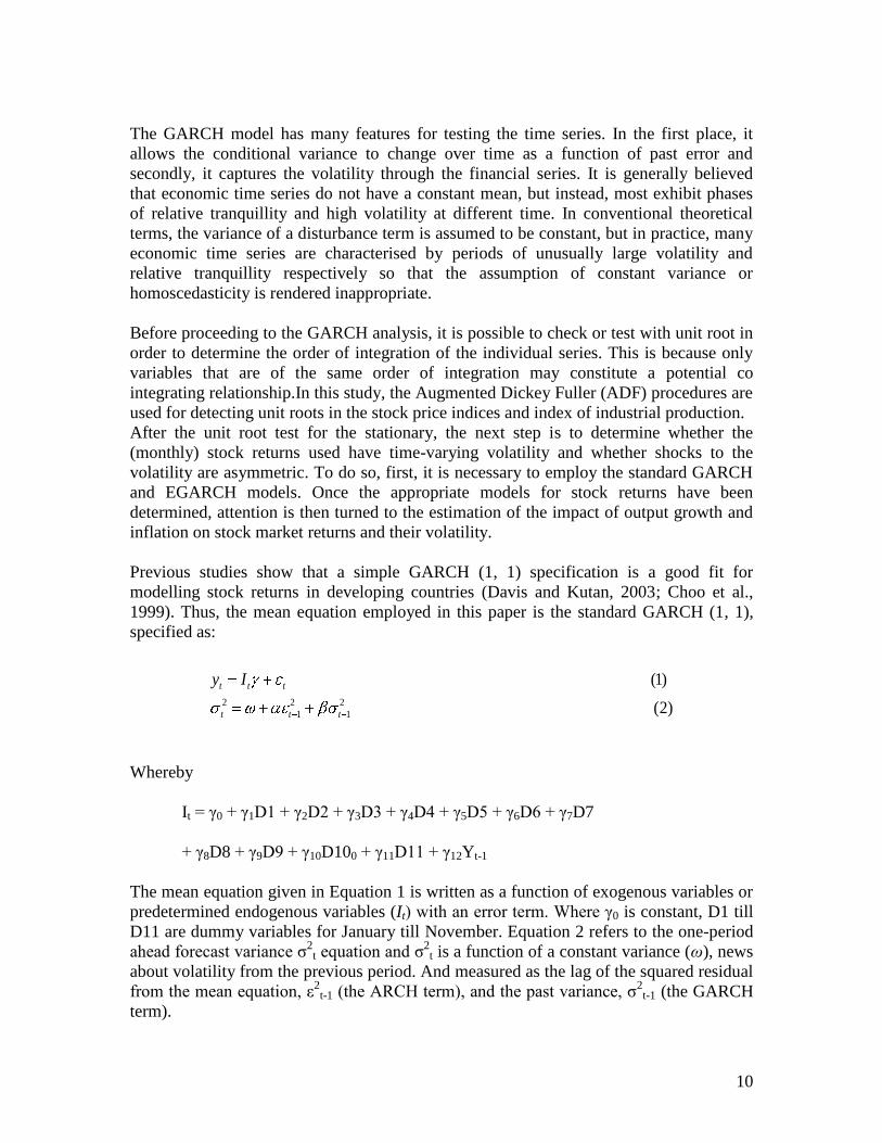
The GARCH model has many features for testing the time series. In the first place, it

allows the conditional variance to change over time as a function of past error and

secondly, it captures the volatility through the financial series. It is generally believed

that economic time series do not have a constant mean, but instead, most exhibit phases

of relative tranquillity and high volatility at different time. In conventional theoretical

terms, the variance of a disturbance term is assumed to be constant, but in practice, many

economic time series are characterised by periods of unusually large volatility and

relative tranquillity respectively so that the assumption of constant variance or

homoscedasticity is rendered inappropriate.

Before proceeding to the GARCH analysis, it is possible to check or test with unit root in

order to determine the order of integration of the individual series. This is because only

variables that are of the same order of integration may constitute a potential co

integrating relationship.In this study, the Augmented Dickey Fuller (ADF) procedures are

used for detecting unit roots in the stock price indices and index of industrial production.

After the unit root test for the stationary, the next step is to determine whether the

(monthly) stock returns used have time-varying volatility and whether shocks to the

volatility are asymmetric. To do so, first, it is necessary to employ the standard GARCH

and EGARCH models. Once the appropriate models for stock returns have been

determined, attention is then turned to the estimation of the impact of output growth and

inflation on stock market returns and their volatility.

Previous studies show that a simple GARCH (1, 1) specification is a good fit for

modelling stock returns in developing countries (Davis and Kutan, 2003; Choo et al.,

1999). Thus, the mean equation employed in this paper is the standard GARCH (1, 1),

specified as:

Whereby

It = γ0 + γ1D1 + γ2D2 + γ3D3 + γ4D4 + γ5D5 + γ6D6 + γ7D7

+ γ8D8 + γ9D9 + γ10D100 + γ11D11 + γ12Yt-1

The mean equation given in Equation 1 is written as a function of exogenous variables or

predetermined endogenous variables (It) with an error term. Where γ0 is constant, D1 till

D11 are dummy variables for January till November. Equation 2 refers to the one-period

ahead forecast variance σ2

t equation and σ2t is a function of a constant variance (ω), news

about volatility from the previous period. And measured as the lag of the squared residual

from the mean equation, ε2

t-1 (the ARCH term), and the past variance, σ2

t-1 (the GARCH

term).

)2(

)1(

2

1

2

1

2

ttt

ttt Iy

11

The next step is to investigate the predictive power of output growth and inflation on

stock returns and volatility. To do so, Davis and Kutan (2003) used a GARCH

specification to model the conditional variance of stock returns as a function of past

squared forecast errors, past stock returns, and past values of other macroeconomic

variables that may affect the conditional variance. Extending the standard GARCH (1,1)

specification, their model takes the form:

Whereby these models focus on the impact of overall output volatility (covering both

recessions and expansions) on stock market volatility investigated is taken here. In

addition, it include output grow in both the mean and variance equation. Besides that,

they included macroeconomic variables, output and inflation.

3.4 Parameter Estimation and Diagnostics Checking

The diagnostic tests will be employed to test the residuals while the Ljung-Box (LB)

Portmanteau statistic and Lagrange Multiplier (LM) test will be used on the standardised

residual. The LB Q-statistic is computed as follow:

Where rj is the jth autocorrelation and T is the number of observations. Under the null

hypothesis that the first k autocorrelation are zero, the Q-statistic is distributed as chi-

square with degree of freedom equal to the number of lag autocorrelation k. The critical

values were based on the chi-square (χ2) distributions.

Engle proposed the LM to test the ARCH effect. If there are no ARCH effects, the

estimated values of the coefficients of ARCH terms should be zero. So with a sample of

T residuals, under the null hypothesis of no ARCH errors, the test statistic TR2 converges

to chi-square distribution (TR2~ χ

2), whereby T and R

2 are the number of observations

and the coefficient of determination from the auxiliary regression respectively, with

degrees of freedom equal to the number of autoregressive term in the auxiliary

regression. If TR2

is sufficiently large, the rejection of the null hypothesis that a1 through

)4()()(

)3()()(

11

2

1

2

1

2

11

it

k

i

iit

k

i

ittt

tit

k

i

iit

k

i

itt

InflationgrowthOutput

InflationbgrowthOutputaIR

k

jLB

jT

jrTTQ

1

2

)2(

12

aq are jointly equal to zero is equivalent to rejecting the null hypothesis of no ARCH

errors. Likewise, if TR2 is sufficiently low, we conclude that there are no ARCH effects.

In estimating the GARCH (1,1) model, if the constant term is found to be insignificantly

different from zero then the mean assumption is satisfied. Then, serial independence

assumption will be tested by applying LB Q-statistic. If the residuals turn out to be

uncorrelated then this will imply that the returns themselves are uncorrelated. Finally, to

examine whether stock returns are normally distributed, a test of normality based on

skewness and kurtosis (Jarque-Bera) will be applied to the residuals and if the residuals

turn out to be normally distributed the stock returns will be normally distributed, and

hence, the concerned stock market is efficient. In the estimated of the GARCH (1,1) it is

assumed that the α1 + β1 < 1. If α1 + β1 < 1, it is an indication of weakly stationary

GARCH and a measure of volatility of shock in time series returns. In this regard,

Bollerslev argues that GARCH (1,1) is sufficient for most financial series and it is an

important feature as the GARCH can capture volatility clustering evident in financial

time series.

This study uses monthly data of Consumer Price Index (CPI), major stock index or share

prices and Index of Industrial Production (IIP) or Index of Manufacturing Production

(IMP) from five Asian countries namely India, Japan, Korea, Malaysia and Philippines.

All the data were obtained from the International Financial Statistics (IFS) database. The

monthly data are from the period of 1991:1 to middle of 2004. Stock returns, inflation

and real output growth rate are constructed by taking the logarithmic difference of the

stock index, CPI and IIP or IMP, respectively. All variables are computed based on the

log-differenced data, multiplied by 100.

Empirical Results

Table 1: ADF test statistics

Variables India Japan Korea Malaysia Philippine

Stock return -4.88862 -5.14011 -5.13674 -6.48494 -5.64546

Inflation -6.82911 -7.26365 -6.42194 -6.40713 -4.46523

Output Growth -8.39161 -10.8988 -10.3698 -5.88392 -5.73519

5% Critical Value -3.43940 -3.43920 -3.43900 -3.43900 -3.43920

From the above Table 1, we can see that all the absolute t-statistic value for the various

variables series from the five countries is greater than the t-critical value. So, the Ho for

all the series is therefore rejected. This implies that the time series of all country‟s stock

return is stationary. There is no existence of unit root in order zero. We confirm that all

the country‟s time series is I(0). The process of Unit Root test can stop here because a

higher order of differential is not required.

Table 2 reports the descriptive statistics for nominal stock returns, inflation and output

growth. The results indicate that the average monthly stock returns is ranged from

-0.2393% to 1.0332%. Where the highest is India, followed by Malaysia, Korea,

13

Philippine and Japan, but Philippine and Japan average stock returns is in negative during

the sample period. While average inflation ranged from 0.5764% (India) to 0.0265%

(Japan), this shows that high inflation countries such India tends to have higher stock

returns while low inflation countries such as Japan are associated with relatively lower

returns. Malaysia has the highest average output growth during the sample period, with a

monthly growth rate of 0.64%, followed by Korea, India, Japan and Philippine. While

Philippine experienced a negative output growth, -0.0091% in the sample period.

Table 2: Descriptive statistics

Country

Return Inflation Output Growth

Sample

Period Mean Std Dev Mean

Std

Dev Mean Std Dev

India 1.0332 7.8156 0.5764 0.8854 0.4206 6.4256 2:1991 - 5:2004

Japan -0.2393 4.8976 0.0265 0.3639 0.0711 8.1943 2:1991 - 6:2004

Korea 0.0875 8.0073 0.3619 0.4990 0.6085 5.9818 2:1991 - 7:2004

Malaysia 0.2373 0.3087 0.2373 0.3093 0.6416 4.8891 2:1991 - 7:2004

Philippine -0.1066 15.7553 0.5435 0.5128 -0.0091 11.3193 2:1991 - 5:2004 Note: All variables are computed as the log difference between current and previous month‟s observations, multiplied by 100. Std Dev represents standard deviation.

Turning to result for the standard deviation, Philippine has the highest deviation with

respect to the stock returns while the lowest is Malaysia. Inflation is the most volatile in

India with the standard deviation of 0.8854, while other four countries exhibit similar

standard deviations. Philippine has the highest deviation in output growth with standard

deviation 11.3193, while Malaysia has the lowest with 4.8891.

14

-30

-20

-10

0

10

20

30

40

92 94 96 98 00 02 04

INDIA

-20

-10

0

10

20

92 94 96 98 00 02 04

JA P A N

-30

-20

-10

0

10

20

30

92 94 96 98 00 02 04

K ORE A

-0.5

0.0

0.5

1.0

1.5

2.0

92 94 96 98 00 02 04

MA LA Y S IA

-120

-80

-40

0

40

80

92 94 96 98 00 02 04

P HILIP P INE

Figure 1 below shows the flow of the stock returns for the five countries during the

sample period.

Figure 1: Monthly Stock Returns from 1991 - 2004

INDIA JAPAN

KOREA MALAYSIA

PHILIPPINES

15

4.3 Evidence for Time-varying Volatility

After the stationary test, the next process is to choose an appropriate model for the stock

returns. Table 3 reports the estimated coefficients for the standard GARCH (1, 1) as

given by equation 3 and 4.

Table 3: Estimation for the standard GARCH (1,1) model for stock returns.

Country

Mean Equation Conditional Variance Equation

Constant Return (-1) Constant α β

India 3.5968* 0.2651* 9.7756 0.2050 0.6199*

(0.0195) (0.0009) (0.1608) (0.2178) (0.0082)

Japan -0.6248 0.2705* 2.5831 0.1293** 0.7623*

(0.5317) (0.0015) (0.2414) (0.0590) (0.0000)

Korea -0.9384 0.2831* 3.3680 0.1173 0.8188*

(0.5369) (0.0017) (0.3377) (0.2175) (0.0000)

Malaysia 0.3676* 0.1213** 0.0790* 0.2700** -0.4568*

(0.0000) (0.0305) (0.0000) (0.0333) (0.0048)

Philippine 1.2375 0.1260 10.007 0.7033* 0.4918*

(0.5454) (0.1648) (0.1219) (0.0029) (0.0000) Notes: Monthly seasonal dummy variables representing all months but Decembers were included in the mean equation estimations.

The parenthesis figure is p-value. *, **, and *** denote significance level at the 1, 5, and 10%, respectively.

The results clearly suggest that there is indeed significant time-varying volatility in stock

returns during the sample period and a commonly employed GARCH (1,1) specification

seems to be a good fit for all the five countries considered as well. This is because the

beta (β) or GARCH term for the models are all statistically significant at 1% level. The

results further suggests that volatility is persistent as measured by sum of the (α+β) which

is quite high, higher than 0.8 for most of the countries except for Malaysia, which is in

negative sign. This means that the volatility is persistent for the period under study as

exhibited by high significance of the coefficients of ARCH and GARCH terms.

Therefore, two conclusions could be made, firstly, we can predict volatility in the current

period from the previous information, and secondly, the historical prices reflecting the

news or the information. These results are consistent with the conclusion of the Bekaert

and Harvey (1997), Aggarwal et al. (1999), Davis and Kutan (2003), Choo et al. (1999),

and Zhao (1999) where the monthly stock returns exhibits significant time-

varying volatility.

To choose a proper lag length for variables in the mean and variance equation, the

standard GARCH (1,1) models and EGARCH (1,1) model are first estimated from lag

one to lag thirteen. Table 4 reports the Akaike Information Criterion (AIC) based on each

lag selection. The order with the lowest AIC will be chose. The results indicate that India

has the lowest AIC at lag 4, Japan at lag 2, Korea and Malaysia at lag 3 and Philippines at

lag 1. These mean every country will get individual lag order in the mean equation and

variance equation for their GARCH models.

16

Table 4: Lag selection tests: Akaike Information Criteria (AIC)

Order India Japan Korea Malaysia Philippine

1 6.926055 6.092437 6.963621 0.240807 8.229433*

2 6.904894 6.062502* 6.983660 0.250299 8.386922

3 6.921932 6.090998 6.938525* 0.171771* 8.440656

4 6.83296* 6.122003 7.005944 0.227500 8.447447

5 6.924484 6.135464 7.054767 0.229886 8.465818

6 6.914297 6.207423 7.073825 0.262513 8.546484

7 7.014942 6.228467 7.125471 0.242676 8.564168

8 7.053546 6.235342 7.115478 0.329341 8.606027

9 7.068216 6.304321 7.164536 0.313753 8.645002

10 7.086952 6.313375 7.197571 0.412646 8.693480

11 7.094465 6.374827 7.254744 0.406097 8.723528

12 7.125014 6.378665 7.289330 0.467934 8.751555

13 7.074696 6.459364 7.189312 0.484528 8.795720 Notes: The * is the lowest figure among the 13 lags.

Table 5 reports the result for the cumulative impact of changes in the inflation and output

growth on stock returns over a specific period (month) horizon, as per the lag periods

determined. The statistical significance of inflation and output growth is measured by the

chi-square distribution. The χ2 distribution is to test the significance of the sum of the

coefficients for inflation and output growth on stock returns and volatility separately over

an individual lags period. The Bollersler and Wooldridge‟s (1992) robust variance

estimator is employed for computing the standard errors.

Table 5: The cumulative impact of inflation and output growth on stock returns and

volatility

Country

Stock Returns Stock Returns Volatility

Σ Inflation Σ Output Σ Inflation Σ Output

India 0.8362 0.7057 -5.053 -1.799

(24.5688*) (6.1643) (6.7220) (8.0311***)

Japan -1.401 0.2409 -2.0732 -1.2195

(5.1471***) (0.8598) (3.6406) (1.5269)

Korea 0.0747 -0.4335 -1.9345 -1.5491

(1.9783) (1.2166) (8.4795**) (4.4576)

Malaysia 2.6878 -0.0081 0.067 -0.0061

(90.9564*) (1.0526) (5.7172) (1.8639)

Philippine -1.0511 -0.1432 -25.7641 1.5179

(0.1634) (69.4438*) (0.5941) (1.8689***) Notes: The reported coefficients are sum of the lags of inflation and output for stock returns and volatility based on the countries lags

order. The parenthesis is critical values of chi-square distributions for the statistical significance of the sum of the lags coefficients. *,

*, and *** denote significance level at the 1, 5, and 10%, respectively.

17

From the result for average stock returns, it can be observed that inflation has effect on

stock returns in majority countries, which include India, Japan and Malaysia. Note that

the sign of inflation for India and Malaysia is positive while negative for Japan. This

indicates that a 1% increase in inflation increases the stock market for India by 0.8362%

and 2.6878% for Malaysia respectively, but reduces -1.401% for Japan. These results are

consistent with Choudhry (2001) whereby inflation and stock returns are positively

correlated for high inflation countries such as India. In contrary the relationship will be

negative for the countries which have moderate or low inflation, like Japan [Asprem

(1989), Cochran and Defina (1993), Zhao (1999), and Adrangi et al. (1999, 2000)]

though there is a contradiction for Malaysia.

As for the impact of cumulative output growth to the stock returns, there is no evidence

that output growth has effect on stock returns during the period of study except for the

case of Philippines, whereby for every 1% increase in the output growth, there will be a

decrease in the stock returns by 0.1432%. The negative sign of the impact of output

growth is in contradiction with the common finding of the previous studies of Harvey

(1989), Aspreem (1989), Conova and Nicolo (1995), Peiro (1996), Mauro (2003) and

Davis and Kutan (2003). But it is not an isolated finding, sharing the sentiments of Zhao

(1999).

For the variance equation, the results show that the sum of the impact of inflation on the

conditional volatility is not significant in all the countries except for the case of Korea,

which has a negative impact of inflation on the conditional volatility but because of low

inflation rates in Korea, an inflation rate movement tends to have a „calming‟ effect on

volatility. As for the impact of the output growth, only India and Philippine is statistically

significant under 10% significance level. This shows that output movements do not have

overwhelming impact on stock market volatility for this period of study, except for India

and Philippines. Even these two nations have conflicting signs, for Philippines, it is

positive while for India it is negative. The former has relatively higher output volatility

while the latter exhibits lower volatility. This indicates that country with relatively higher

output volatility as Philippine (standard deviation: 11.32) is associated with higher

conditional volatility of stock returns and vice versa, as like India (standard deviation:

6.43).

18

Figure 2 below shows the volatility of monthly stock returns during the sample period for

all the chosen countries.

Figure 2: Monthly stock returns residual

India Japan

-20

-10

0

10

20

30

92 93 94 95 96 97 98 99 00 01 02 03 04

RETURN Residuals

-15

-10

-5

0

5

10

15

92 93 94 95 96 97 98 99 00 01 02 03 04

RETURN Residuals

Korea Malaysia

-30

-20

-10

0

10

20

30

92 93 94 95 96 97 98 99 00 01 02 03 04

RETURN Residuals

-1.0

-0.5

0.0

0.5

1.0

1.5

92 93 94 95 96 97 98 99 00 01 02 03 04

RETURN Residuals

Philippines

-120

-80

-40

0

40

80

92 93 94 95 96 97 98 99 00 01 02 03 04

RETURN Residuals

19

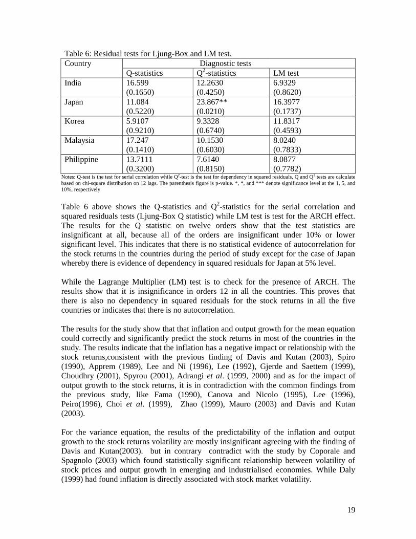
Table 6: Residual tests for Ljung-Box and LM test.

Country Diagnostic tests

Q-statistics Q2-statistics LM test

India 16.599 12.2630 6.9329

(0.1650) (0.4250) (0.8620)

Japan 11.084 23.867** 16.3977

(0.5220) (0.0210) (0.1737)

Korea 5.9107 9.3328 11.8317

(0.9210) (0.6740) (0.4593)

Malaysia 17.247 10.1530 8.0240

(0.1410) (0.6030) (0.7833)

Philippine 13.7111 7.6140 8.0877

(0.3200) (0.8150) (0.7782) Notes: Q-test is the test for serial correlation while Q2-test is the test for dependency in squared residuals. Q and Q2 tests are calculate

based on chi-square distribution on 12 lags. The parenthesis figure is p-value. *, *, and *** denote significance level at the 1, 5, and

10%, respectively

Table 6 above shows the Q-statistics and Q2-statistics for the serial correlation and

squared residuals tests (Ljung-Box Q statistic) while LM test is test for the ARCH effect.

The results for the Q statistic on twelve orders show that the test statistics are

insignificant at all, because all of the orders are insignificant under 10% or lower

significant level. This indicates that there is no statistical evidence of autocorrelation for

the stock returns in the countries during the period of study except for the case of Japan

whereby there is evidence of dependency in squared residuals for Japan at 5% level.

While the Lagrange Multiplier (LM) test is to check for the presence of ARCH. The

results show that it is insignificance in orders 12 in all the countries. This proves that

there is also no dependency in squared residuals for the stock returns in all the five

countries or indicates that there is no autocorrelation.

The results for the study show that that inflation and output growth for the mean equation

could correctly and significantly predict the stock returns in most of the countries in the

study. The results indicate that the inflation has a negative impact or relationship with the

stock returns,consistent with the previous finding of Davis and Kutan (2003), Spiro

(1990), Apprem (1989), Lee and Ni (1996), Lee (1992), Gjerde and Saettem (1999),

Choudhry (2001), Spyrou (2001), Adrangi et al. (1999, 2000) and as for the impact of

output growth to the stock returns, it is in contradiction with the common findings from

the previous study, like Fama (1990), Canova and Nicolo (1995), Lee (1996),

Peiro(1996), Choi et al. (1999), Zhao (1999), Mauro (2003) and Davis and Kutan

(2003).

For the variance equation, the results of the predictability of the inflation and output

growth to the stock returns volatility are mostly insignificant agreeing with the finding of

Davis and Kutan(2003). but in contrary contradict with the study by Coporale and

Spagnolo (2003) which found statistically significant relationship between volatility of

stock prices and output growth in emerging and industrialised economies. While Daly

(1999) had found inflation is directly associated with stock market volatility.

20

It can be concluded that only inflation has impact on the stock returns in most countries

in study, but not for output growth. Except for Korea and Philippine which inflation and

output growth has significance effect on stock returns volatility, respectively, all the

remaining countries have insignificant relationship.

Conclusion

The main objective of this study is to examine the predictive power of the inflation and

output growth to the stock returns and volatility in five Asian countries. While previous

studies have studied the relationship between macroeconomic factors and stock return

and volatility. But most of them have not placed real output and inflation together as

exogenous variables in both the mean and conditional variance equations to

simultaneously estimate of the effect of these variables on the first and second moments

of stock market returns. By using GARCH model, this study places real output and

volatility in the same forecasting model accounts for time-varying volatility in returns for

these five countries.

The findings suggest that for India, Korea and Malaysia, inflation has significant

predictive power for stock return over the individual horizon period. While for the output

growth, only Philippine is significance under 1% level. But for the stock returns

volatility, only India and Philippine output growth, and Korea inflation rate have

significance effect to the predictive power for stock return volatility.

21

References

Adrangi, B., Chatrath, A., and Raffiee, K. (1999). Inflation, Output and Stock Prices:

Evidence from Two Major Emerging Markets. Journal of Economics and Finance, 23

(3), 266-278.

Aggrarwal, R., Inclan, C., and Leal, R. (1999). Volatility in Emerging Stock Markets.

Journal of Financial and Quantitative Analysia, 34, 33-55.

Asprem, M. (1989). Stock prices, asset portfolio and macroeconomic variable in ten

European countries. Journal of Banking and Finance, 13, 589-612.

Balvers, R.J, Cosmano, T.F., and McDonald, B. (1990). Predicting Stock Returns in an

Efficient Market. The Journal of Finance, 45 (4), 1109-1128.

Bekaert, G. and Harvey, C.R. (1997). Emerging equity market volatility. Journal of

Financial Economics, 43, 29-77.

Binswanger, M. (2000). Stock market booms and real economic activity: Is this time

different? International Review of Economics and Finance, 9, 387-415.

Bollerslev, T. (1986). Generalized Autoregressive Conditonal Heteroscedasticity. Journal

of Econometrics, 31, 307-327.

Canova F., and Nicolo, G.D. (1995). Stock returns and real activity: A structural

approach. European Economic Review, 39, 981-1015.

Caporale, G.M., and Spagnolo, N. (2003). Asset prices and output growth volatility: the

effects of financial crises. Economics Letter, 79, 69-74.

Choi, J.J., Hauser, S., and Kopecky, K.J. (1999). Does the stock market predict real

activity? Time Series evidence from the G-7 countries. Journal of Banking and

Finance, 23, 1771-1792.

Choo, W. C., Muhammad Idress, A., and Mat Yusoff, A. (1999). Performamnce of

GARCH models in forecasting stock market volatility. Journal of Forecasting, 18(5),

333-343.

Choudhry, T. (2001). Inflation and rates of returns on stocks: evidence from high

inflation countries. Journal of International Financial Markets, Institutions and

Money, 11, 75-96.

Cochrane, S.j., and Define, R.H. (1993). Inflation negative effects on real stock prices:

new evidence and a test of the proxy effect hypothesis. Applied Economics, 25, 263-

274.

Cutter, D.M., Poterba, J.M., and Summers, L.H. (1989). What Move Stock Prices. The

Journal of Portfolio Management, 4-11.

Daly, K. (1999). Financial Volatility and Real Economic Activity. Singapore: Ashgate.

Davis,N., and Kutan, A.M. (2003). Inflation and output as predictors of stock returns and

volatility: International evidence. Applied Financial Economics, 13, 693-700.

Engle, R.F. (1982). Autoregressive Conditional Heteroscedasticity with estimates of the

variance of UK inflation. Econometrica, 50, 987-1008.

Engle, R.F. (1983). Estimates of the variance of U.S. inflation based upon the ARCH

model. Journal of Money, Credit and Banking, 15, 286-301.

Engle, R.F., and Ng, V.K. (1993). Measuring and testing the impact of news on volatility.

Journal of Finance, 1(5), 1749-1778.

Engle, R.F., Lilien, D.M., and Robbins, R.P. (1987). Estimating time varying risk premia

in the term structure: the ARCH-M model. Econometrica, 55, 391-407.

22

Fama, E. (1981). Stock returns, real activity, inflation and money. American Economic

Review, 71, 545-64.

Fama, E. (1990). Stock returns, expected returns, and real activity. Journal of Finance,

45, 1089-1108.

French, K.R., Schwert, G.W., and Stambaugh, R.F. (1987). Expected stock returns and

volatility. Journal of Financial Economics, 19, 3-29.

Gjerde, Ø., and Sættem, F. (1999). Causal relation among stock returns and

macroeconomic variables in a small open economy. Journal of International

Financial Markets, Institutions and Money, 9, 61-74.

Guo, H. (2002). Stock Market Returns, Volatility, and Future Output. The Federal

Reserve Bank of St. Louis, 75-82.

Harvey, C.P. (September 1989). Forecasts of Economic Growth From The Based and

Stock Market. Financial Analysts Journal, 38-45.

Hess, P.J., and Lee, B. (1999). Stock Returns and Inflation with Supply and Demand

Disturbances. The Review of Financial Studies, 12 (5), 1203-1218.

Kaul, G. (1987). Stock returns and inflation: the role of the monetary sector. Journal of

Financial Economics, 18, 253-276.

Kim, D., and Kon, S.J. (alternative models for the conditional heteroscedasticity of stock

returns. Journal of Business, 67 (4), 563-598

Lamoureux, C.G., and Lastrapes, W.D. (1990). Heteroscedasticity in stock return data:

volume versus GARCH effects. Journal of Finance, 45 (1), 221-229.

Lee, Bong-Soo (1992). Causal Relationship among Stock Returns, Interest Rates, Real

Activity, and Inflation. The Journal of Finance, 47 (4), 1591-1603.

Lee, K. (1996). Long-term output growth as a predictor of stock returns, Applied

Financial Economics, 6, 421-432.

Liu, X., Romilly, P., and Song, H. (1998). Stock returns and volatility: An empirical

study of Chinese Stock Market. International Review of Applied Economics, 12 (1),

129-140.

Mauro, P. (2003). Stock returns and output growth in emerging and advanced economies.

Journal of Development Economics, 71, 129-153.

Park, Sangkyun (1997). Rationary of negative stock price responses to strong economic

activity. Financial Analysts Journal, 52-56.

Peiro, Amado (1996). Stock Prices, Production and Interest Rates: Comparison of Three

European Countries with the USA. Empirical Economics, 21, 221-234.

Pena, J.I., Restoy, F., and Rodriguez, R. (2002). Can output explain the predictability

and volatility of stock returns. Journal of International Money and Finance, 21, 163-

182.

Rangvid, Jesper (2001). Predicting return and changes in real activity: evidence from

emerging economies. Emerging Markets Review, 2, 309-329.

Schwert, G.W. (1990). Stock Returns and Real Activity: A century of Evidence. The

Journal of Finance, 45 (4), 1237-1257.

Schwert, G.W., and Seguin, P.J. (1990). Heteroscedasticity in stock returns. Journal of

Finance, 45 (4), 1129-1155.

Spiro, P.S. (1990). The important of internal rate changes on stock price volatility. The

Journal of Portfolio Management, 63-68.

23

Spyrou, S.I. (2001). Stock returns and inflation: evidence from emerging market. Applied

Economics Letters, 8, 447-450.

Wilson, J.W., and Jones, C.P. (1987). Common stock prices and inflation: 1857-1985.

Financial Analysts Journal, 67-72.

Wooldrige, J.M. (2003). Introductory Econometrics: A Modern Approach (2 ed.).

Singapore: Thomson South-Western.

Zhao, Xing-Qiu (1999). Stock prices, inflation and output: Evidence from China. Applied

Economics Letter, 6, 509-511.