A seminAr on

DigitAl signAl processing Architectures

moDule -3

topic : - multirAte Dsp

by

Sagar p. Sangale

Introduction

Multirate systems have gained popularity since the early 1980s and they

are commonly used for audio and video processing, communications

systems, and transform analysis. In most applications Multirate systems are

used to improve the performance, or for increased computational

efficiency. The two basic operations in a Multirate system are decreasing

(decimation) and increasing (interpolation) the sampling-rate of a signal.

Multirate systems are sometimes used for sampling-rate conversion, which

involves both decimation and interpolation.

Multirate Signal Processing Sampling rate conversion: The process of converting

a signal from a given rate to a different rate. Multirate Systems: Systems handling more than one

sampling rate. Objective: Minimize the complexity of the signal

processing under Nyquist Sampling criterion. Key Operations: Sampling rate conversion for

communications.-- Decimation: Down sampling at receiver side-- Interpolation: Up sampling at transmission side

DSP Functions:Decimation FilteringInterpolation Filtering

Why and Where to Use Multirate

Multirate systems can reduce required system computation, bandwidth, or storage requirements.

Multirate systems are used for converting data between A/D and D/A devices that run at different sampling rates.

Common Multirate applications: Sampling systems Audio/speech encoders Image/video encoders Music synthesizers image systems Echo cancellers Modems, data multiplexers

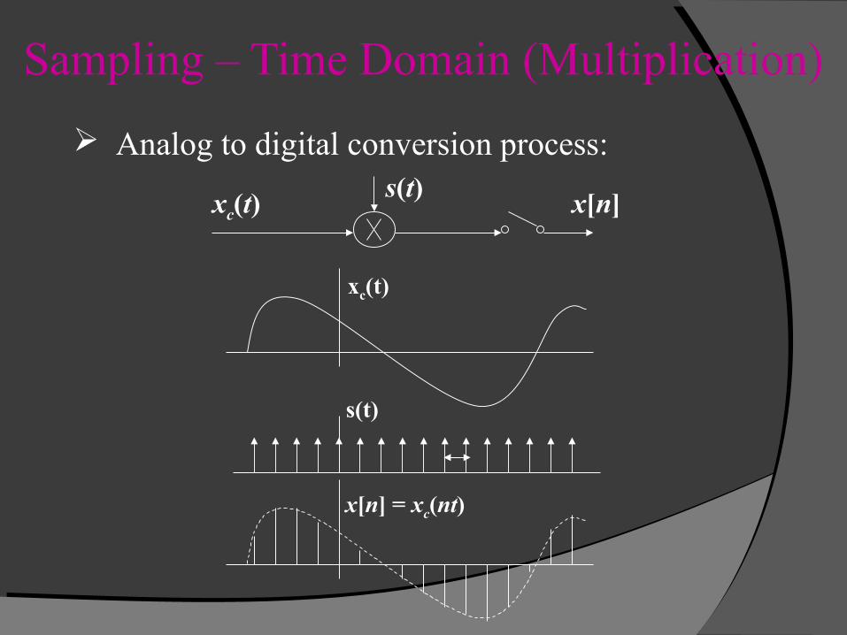
Sampling – Time Domain (Multiplication)

xc(t)s(t)

x[n]

Analog to digital conversion process:

x[n] = xc(nt)

xc(t)

s(t)

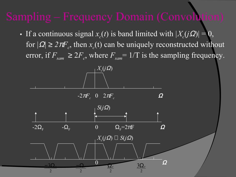
Sampling – Frequency Domain (Convolution)

S(jΩ)

Xc(jΩ) ⊗ S(jΩ)

Ω

Ω

Ω2πFc-2πFc 0

0

0

ΩF=2πF-ΩF-2ΩF

23Ω− F

23ΩF

2Ω− F

2ΩF

• If a continuous signal xc(t) is band limited with |Xc(jΩ)| = 0, for |Ω| ≥ 2πFc, then xc(t) can be uniquely reconstructed without error, if Fsam ≥ 2Fc, where Fsam= 1/T is the sampling frequency.

Xc(jΩ)

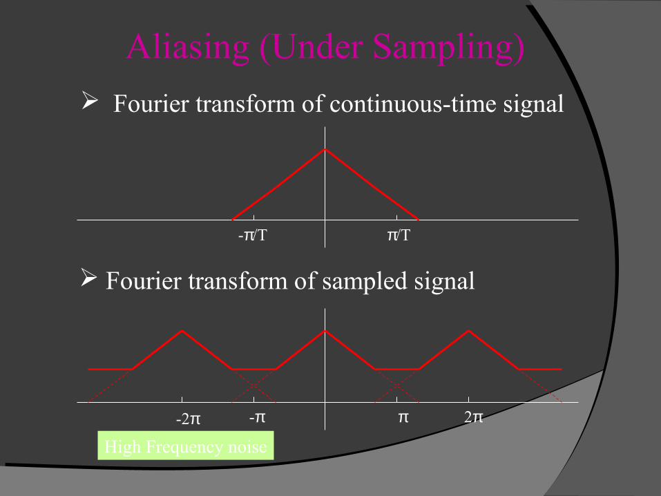
Aliasing (Under Sampling)

π 2π-π-2π

π/T-π/T

Fourier transform of continuous-time signal

Fourier transform of sampled signal

High Frequency noise

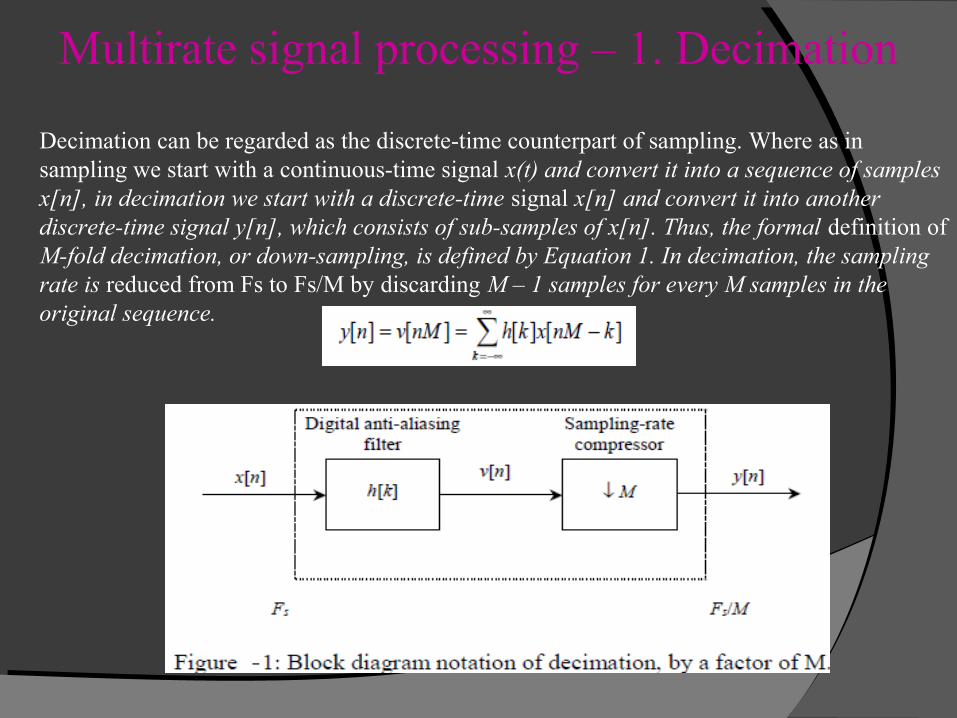
Multirate signal processing – 1. Decimation

Decimation can be regarded as the discrete-time counterpart of sampling. Where as in sampling we start with a continuous-time signal x(t) and convert it into a sequence of samples x[n], in decimation we start with a discrete-time signal x[n] and convert it into another discrete-time signal y[n], which consists of sub-samples of x[n]. Thus, the formal definition of M-fold decimation, or down-sampling, is defined by Equation 1. In decimation, the sampling rate is reduced from Fs to Fs/M by discarding M – 1 samples for every M samples in the original sequence.

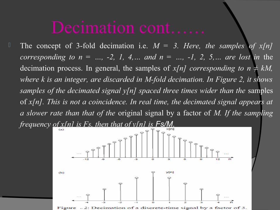
Decimation cont…… The concept of 3-fold decimation i.e. M = 3. Here, the samples of x[n]

corresponding to n = …, -2, 1, 4,… and n = …, -1, 2, 5,… are lost in the

decimation process. In general, the samples of x[n] corresponding to n ≠ kM,

where k is an integer, are discarded in M-fold decimation. In Figure 2, it shows

samples of the decimated signal y[n] spaced three times wider than the samples

of x[n]. This is not a coincidence. In real time, the decimated signal appears at

a slower rate than that of the original signal by a factor of M. If the sampling

frequency of x[n] is Fs, then that of y[n] is Fs/M.

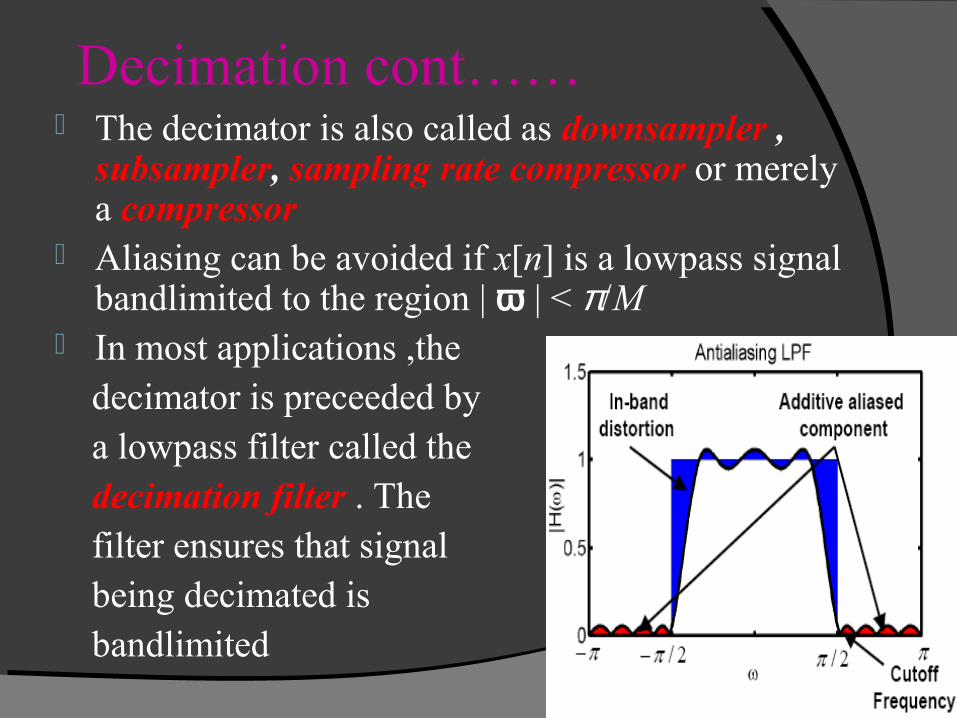
Decimation cont…… The decimator is also called as downsampler ,

subsampler, sampling rate compressor or merely a compressor

Aliasing can be avoided if x[n] is a lowpass signal bandlimited to the region | ω | < π/M

In most applications ,the decimator is preceeded by a lowpass filter called the decimation filter . The filter ensures that signal being decimated is bandlimited

2.Interpolation Interpolation is the exact opposite of decimation. It is an information preserving operation, in that all samples of x[n] are present in the expanded signal y[n]. The mathematical definition of L-fold interpolation is defined by Equation .2 and the block diagram notation is depicted in Figure 3 Interpolation works by inserting (L–1) zero-valued samples for each input sample. The sampling rate therefore increases from Fs to LFs. With reference to Figure 3, the expansion process is followed by a unique digital low-pass filter called an anti-imaging filter. Although the expansion process does not cause aliasing in the interpolated signal.

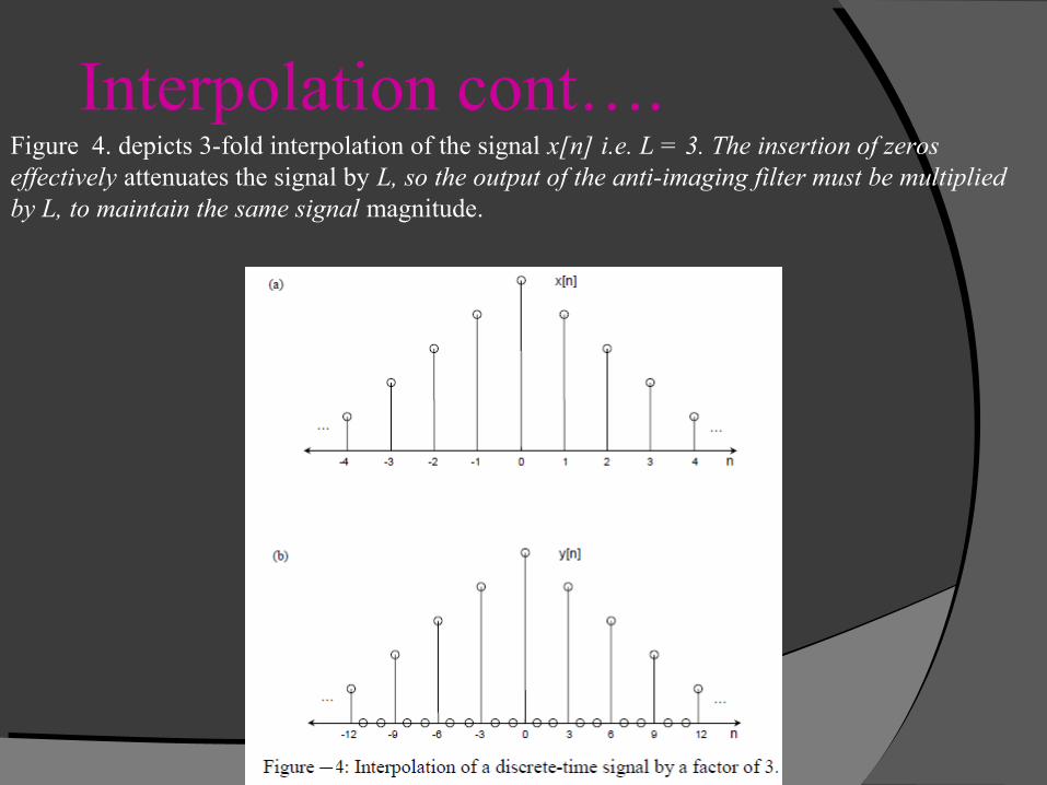
Interpolation cont….Figure 4. depicts 3-fold interpolation of the signal x[n] i.e. L = 3. The insertion of zeros effectively attenuates the signal by L, so the output of the anti-imaging filter must be multiplied by L, to maintain the same signal magnitude.

Sampling Rate Conversion

It is often advantages to digitally alter the sampling rate during processing, after the initial A/D conversion has been finished:High sampling rates (perhaps many times the

Nyquist rates) can be used to help remove noise and quantization error

Low sampling rates (near the Nyquist rate) are best for computation speed and memory requirements

Sampling Rate Conversion cont…

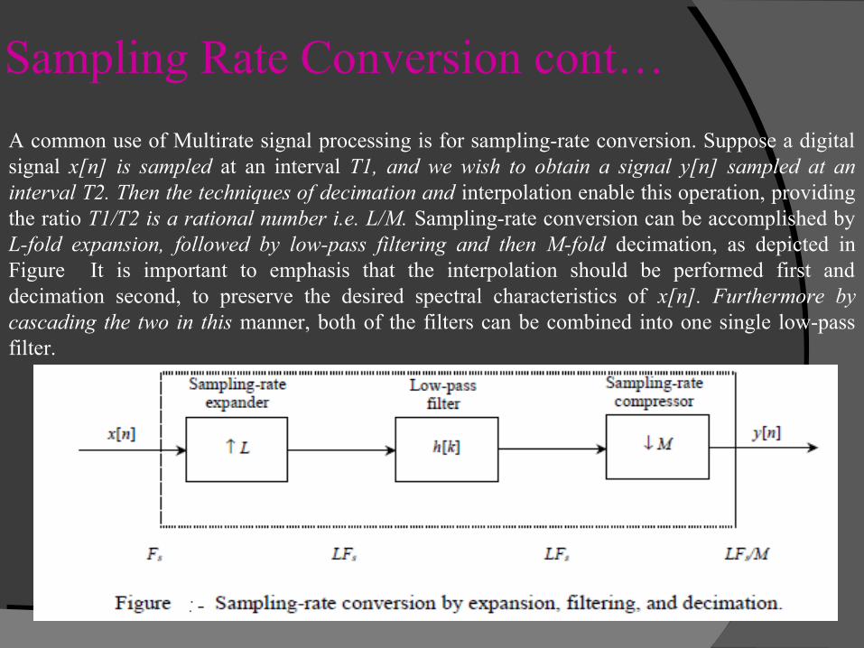
A common use of Multirate signal processing is for sampling-rate conversion. Suppose a digital signal x[n] is sampled at an interval T1, and we wish to obtain a signal y[n] sampled at an interval T2. Then the techniques of decimation and interpolation enable this operation, providing the ratio T1/T2 is a rational number i.e. L/M. Sampling-rate conversion can be accomplished by L-fold expansion, followed by low-pass filtering and then M-fold decimation, as depicted in Figure It is important to emphasis that the interpolation should be performed first and decimation second, to preserve the desired spectral characteristics of x[n]. Furthermore by cascading the two in this manner, both of the filters can be combined into one single low-pass filter.

Sampling Rate Conversion cont…An example of sampling-rate conversion would take place when data from a CD is transferred onto a DAT. Here thesampling-rate is increased from 44.1 kHz to 48 kHz. To enable this process the non-integer factor has to be approximated by a rational number:[L/M=48/44.1]=>[160/147]=>1.088444Hence, the sampling-rate conversion is achieved by interpolating by L i.e. from 44.1 kHz to [44.1x160] = 7056 kHz. Then decimating by M i.e. from 7056 kHz to [7056/147] = 48 kHz.

When the sampling-rate changes are large, it is often better to perform the operation in multiple stages, where Mi(Li), an integer, is the factor for the stage i.M = M1M2…MI or L = L1L2…LI

The multistage approach allows a significant relaxation of the anti-alias and anti-imaging filters, with a consequent reduction in the filter complexity. The optimum number of stages is one that leads to the least computational effort in terms of either the multiplications per second (MPS), or the total storage requirement (TSR).

Thank you………………!!!!!!!!!