Multivariate Tests for Autocorrelation in the Stable and ... 2003 coference in... · Multivariate...
27
Multivariate Tests for Autocorrelation A. Hatemi-J 1 Multivariate Tests for Autocorrelation in the Stable and Unstable VAR Models 1 Abdulnasser Hatemi-J Department of Statistics, Lund University and Department of Economics, University of Skövde, 2 Abstract This study investigates the size and power properties of three multivariate tests for autocorrelation — namely portmanteau test, Lagrange Multiplier (LM) test and Rao F- test — in the stable and unstable vector autoregressive (VAR) models, with and without autoregressive conditional heteroscedasticity (ARCH) using Monte Carlo experiments. Many combinations of parameters are used in the simulations to cover a wide range of situations in order to make the results more representative. The results of conducted simulations show that all three tests perform quite well in stable VAR models without ARCH. In unstable VAR models portmanteau test has serious size distortions. LM and Rao tests perform very well in unstable VAR models without ARCH. These results are true irrespective of sample size or order of autocorrelation. Another clear result that the simulations show is that none of the tests have correct size when ARCH is present irrespective of VAR models being stable or unstable and regardless of the sample size or order of autocorrelation. The portmanteau test seems to have slightly better power properties than the LM test in almost all scenarios. Running title: Multivariate Tests for Autocorrelation in Stable and Unstable VAR Models JEL Classification: C32, C30 Keywords: VAR, Autocorrelation, Monte Carlo Simulations, ARCH, Stability 1 This paper was presented at the 2002 Conference for Econometric Modelling in Pretoria, 3-5 July. The author would like to thank the participants of the conference for their useful comments, especially Peter C. B. Phillips. The usual disclaimer applies. 2 Comments are very welcome. Corresponding address: Department of Economics, University of Skövde, P.O. Box 408, SE-541 28, Skövde, Sweden. Tel: +46 500 44 87 31, E-mail: [email protected] Home page: http://www.his.se/ish/personal/personliga_sidor/abdulnasser_hatemi.htm
Transcript of Multivariate Tests for Autocorrelation in the Stable and ... 2003 coference in... · Multivariate...

Multivariate Tests for Autocorrelation A. Hatemi-J
1
Multivariate Tests for Autocorrelation in the Stable and Unstable VAR Models1
Abdulnasser Hatemi-J
Department of Statistics, Lund University and Department of Economics, University of Skövde,2
Abstract
This study investigates the size and power properties of three multivariate tests for autocorrelation — namely portmanteau test, Lagrange Multiplier (LM) test and Rao F-test — in the stable and unstable vector autoregressive (VAR) models, with and without autoregressive conditional heteroscedasticity (ARCH) using Monte Carlo experiments. Many combinations of parameters are used in the simulations to cover a wide range of situations in order to make the results more representative. The results of conducted simulations show that all three tests perform quite well in stable VAR models without ARCH. In unstable VAR models portmanteau test has serious size distortions. LM and Rao tests perform very well in unstable VAR models without ARCH. These results are true irrespective of sample size or order of autocorrelation. Another clear result that the simulations show is that none of the tests have correct size when ARCH is present irrespective of VAR models being stable or unstable and regardless of the sample size or order of autocorrelation. The portmanteau test seems to have slightly better power properties than the LM test in almost all scenarios. Running title: Multivariate Tests for Autocorrelation in Stable and Unstable VAR Models JEL Classification: C32, C30 Keywords: VAR, Autocorrelation, Monte Carlo Simulations, ARCH, Stability
1 This paper was presented at the 2002 Conference for Econometric Modelling in Pretoria, 3-5 July. The author would like to thank the participants of the conference for their useful comments, especially Peter C. B. Phillips. The usual disclaimer applies. 2 Comments are very welcome. Corresponding address: Department of Economics, University of Skövde, P.O. Box 408, SE-541 28, Skövde, Sweden. Tel: +46 500 44 87 31, E-mail: [email protected] Home page: http://www.his.se/ish/personal/personliga_sidor/abdulnasser_hatemi.htm
Multivariate Tests for Autocorrelation A. Hatemi-J
2
1. Introduction In order to be able to draw valid inference based on the estimated parameters in a
regression model it is important that the error terms are white noise, i.e. expected zero mean, no autocorrelations, constant variance, and normal distribution of errors. In applied work it has usually been assumed that these assumptions are fulfilled without explicitly testing for them. Since the pioneering work by Durbin and Watson (1950) diagnostic testing has been increasingly emphasized in the literature.3 The assumption of no autocorrelation in time series analysis can be invalidated since observations are usually time dependent. In the literature several tests have been developed to test for autocorrelation both singlewise and systemwise. The purpose of this study is to investigate the performance (regarding size and power) of the portmanteau test (Ljung and Box (1978)), Lagrange Multiplier (LM) test (Breusch (1978), Godfrey (19789), and Rao (1973) F-test for autocorrelation in the vector autoregressive (VAR) model in different situations like stability and instability, moderate or small sample sizes, and with and without conditional heteroscedasticity. To the author’s best knowledge the properties of these tests in the multivariate case have not been investigated for unstable and heteroscedastic cases. Since these conditions are usually present when time series data are used, more research on this important issue is warranted. The portmanteau and LM tests are the most applied tests for autocorrelation in the VAR models and more information about their properties can be useful for applied research. According to Edgerton and Shukur (1999) Rao test performs well for system of simultaneous equations. For this reason we also investigate the properties of this test in several circumstances that were not investigated by Edgerton and Shukur (1999). A comparison of the results of the current study with that previous study will be made. Monte Carlo simulation techniques for this purpose will be applied using GAUSS. 4
This study focuses on the size and power of each test in each situation. It is well
known in the literature that the data generating process for many time-series may be characterized by stochastic trends that result in unstable VAR models. Thus, it is of paramount importance to investigate the properties of different tests when the VAR model is stable or not. Since the seminal work by Engle (1982) it is also well known that many time series (specially in the field of financial economics, but also many macro-aggregates like inflation rates and exchange rates) possess occasional periods of high volatility that are time dependent. For this reason it is also important to check the performance of tests for autocorrelation in situations of conditional heteroscedasticity in addition to homoscedastic cases.
This paper is structured as follows. Section 2 will present the portmanteau test,
Breusch-Godfrey test and Rao test. In Section 3 describes the Monte Carlo simulation
3 According to Hendry and Mizon (1999) DW test is only powerful with correct size when all independent variables in the regression are weakly exogenous. However, this test has wrong size and low power when a lagged dependent variable is present in the model as in our case. See also Durbin (1970). It should be mentioned that DW test can be applied only for autocorrelation of degree one. Our focus of interest is autocorrelation higher than degree one in this study. 4 We would like to thank David Edgerton for providing his useful procedures written in GAUSS. We also would like to thank Scott Hacker for his programming support. His excellent skills in programming have made the simulations possible.

Multivariate Tests for Autocorrelation A. Hatemi-J
3
procedure. Section 4 presents the estimated results. Conclusions will be provided in the last Section. Tables are presented in the Appendix.
2. The Portmanteau, LaGrange Multiplier and Rao Tests This section presents three multivariate tests for autocorrelation starting with the
portmanteau test, which was introduced by Box and Pierce (1970) and Ljung and Box (1978). Most economic data consist of time series and the error terms in the model are very often dependent on each other for successive time periods. This is known as the problem of autocorrelation and the reason can be omitted variables, misspecification of the dynamic process, etc. The commonly used statistic for testing the presence of autocorrelation is the Durbin-Watson (D-W) statistic. The D-W tests only for autocorrelation of the first order, and it is not valid in dynamic models. Box and Pierce (1970), suggest the Q-statistic, which looks at not just the first-order autocorrelation but autocorrelations of all orders. Ljung and Box (1978) extended the Q test statistic to adjust for small sample sizes. This test was originally developed to test for autocorrelation in an single equation. This study will, however, considers Ljung-Box test for VAR models in a system perspective. Consider the following k-dimensional VAR model of order L:
tLtLtt yAyAy εν ++++= −− K11 , (1)
where yt is k×1 vector of variables, L is the maximum lag in the VAR model5, v is a k×1 vector of constants, Ai is a k×k matrix of parameters corresponding to lag order i (i = 1, …,
L), and ( )′kt1t ..., , = εεε t denotes the vector of error terms that are assumed to be white noise. To test the null hypothesis that εt is independent of stt −− εε ,,1 L the Ljung-Box portmanteau test for autocorrelation can be applied. This test statistic in its multivariate form is defined as the following according to Hosking (1980):
( ) { } 2)(
1
1000
1000 ~12)( Lsk
s
jjj CCCCtr
jTTTsLB −
=
−−∑ ′−
+= χ , (2)
where
∑+=
−− ′=
T
jtjttj TC
1
10 εε . (3)
Under the null hypothesis (of independence) the Ljung-Box test statistic has approximately a 2χ distribution with k2(s-L) degrees of freedom. Here T is the length of the series, and s denotes the order of autocorrelation. It is important to note that the test can be implemented only when the order of autocorrelation is higher than the lag length in the VAR model, i.e. Ls > .
5 For a new information criterion to choose the lag order in the stable and unstable VAR models see Hatemi-J (2002).

Multivariate Tests for Autocorrelation A. Hatemi-J
4
Another test that is commonly used to test for autocorrelation is the Breusch-Godfrey (See Breusch, 1978, and Godfrey, 1978) LM test statistic. This test can be utilized to test for any autocorrelation order at any significance level. It can also be used to test for autocorrelation in dynamic models. The test is based on the following auxiliary regression:
tststLtktt uyAyAv +++++++= −−−− ερερε KK 1111 . (4) where ut is an error term which is assumed to be white noise. The null hypothesis of no multivariate autocorrelation of degree s is 021 ==== s0 :H ρρρ L and the alternative hypothesis is 0,,0,0 21 ≠≠≠ s1 or :H ρρρ L . There are several test statistics available in the literature that can be used to test the above null hypothesis. According to Edgerton and Shukur (1999) Rao’s F-test (Rao, 1973) has the best performance for autocorrelation of order one in system of equations for stationary variables. This test is of the following form:
),(~11
φφ qFUq
RAO x
−
= (5)
where
rx −∆=φ , (6) ]1)1([½))1(( −−+−+−=∆ skskk kT , (7)6
r q= −2 1, (8) and
U
R
CC
U = . (9)
It should be pointed out that q = 2ks × is the number of restrictions that will be tested under 0H . Note that CR is the estimated variance covariance matrix of the residuals in equation (4) when null hypothesis is imposed and CU is the estimated variance covariance matrix of the residuals in equation (4) when null hypothesis is not imposed. It should be mentioned that:
5)1(4
22
2
−+−=
skqx . (10).
RAO is approximately distributed as F(q, φ) under the null hypothesis, and is equivalent to a standard F statistic when the number of equations is one, i.e. k = 1.
6 Here we have adjusted for the numbers of parameters following by making use of Edgeworth expansion suggested by Anderson (1958). This adjustment was used by Edgerton and Shukur (1999) also.

Multivariate Tests for Autocorrelation A. Hatemi-J
5
However, the multivariate LaGrange Multiplier (LM) test is used extensively in the literature because it is simpler to estimate and several econometric packages have an automatic procedure to estimate the LM test. For this reason we will also examine the properties of the LM test. This test is defined as follows according to Johansen (1996):
( ) 2~log ksU
RCC
sLM ×
∆= χ (11)
∆ is defined in equation (7). Under the null hypothesis of no serial correlation of order s, the LM statistic is asymptotically distributed as 2χ with s×k2 degrees of freedom.
3. Monte Carlo Simulation The focus of this study is on a bivariate VAR(1) model with autocorrelation of second degree described below:
+
×
+
=
−
−
t2
t1
1t2
1t1
22,121,1
12,111,1
t2
t1
yy
0.10.1
yy
εε
αααα
, (12)
and
+
×
+
×
=
−
−
−
−
t
t
t
t
t
t
t
t
uu
2
1
22
21
22,221,2
12,211,2
12
11
22,121,1
12,111,1
2
1
εε
ρρρρ
εε
ρρρρ
εε
(13)
The variance-covariance matrix of the error terms vector (εt) is assumed to be normally distributed. Under the null hypothesis of no autocorrelation all of the parameter matrixes in equation (13) are zero matrixes and εt = ut. We run thousands of simulations assuming the null hypothesis is true with different values for the parameters in equation (12) to determine how close the actual size (the simulation-based rejection rate under the null hypothesis) of each test statistic is to its nominal (asymptotically-based) size. We also run thousands of simulations assuming nonzero values for the parameters in equation (13) to check the power. In some simulations we assume constant variance in the errors and in others we assume the following autoregressive conditional heteroscedasticity (ARCH) process describes the variance of the errors:
[ ][ ]
[ ][ ]
×
+
×
−
−=
−
−
−
−2
12
211
22
11
2
1
22
11
122
111
00
0.1000.1
||
t
t
t
t
tt
tt
bb
VarVar
bb
VarVar
εε
εε
εεεε
. (14)
This formulation is based on a simple version of Engle’s ARCH model following Greene (2001) presented below:
[ ] 21
2110 −+×= ttt bbw εε (15)

Multivariate Tests for Autocorrelation A. Hatemi-J
6
Here wt is assumed to be standard normal. By using the above equation we can see that the conditional mean of εt is zero, i.e.:
[ ] ,0| 1 =−ttE εε (16) and the conditional variance is defined as:
[ ] [ ] [ ] [ ] 2110
2110
21
21 || −−−− +=+×== ttttttt bbbbwEEVar εεεεεε (17)
thus, conditional on εt-1, εt is heteroscedastic. The unconditional variance of εt is equal to the following:
[ ] [ ][ ] [ ] [ ]110
21101| −−− +=+== ttttt VarbbEbbVarEVar εεεεε (18)
Assuming that the data generating process for the error terms is characterized by variance stationarity then the unconditional variance is not changing across time. Hence, we can write the following relationship:
[ ] [ ] [ ]1
01101 1 b
bVarbbVarVar ttt −
=+== −− εεε (19)
This equation makes it possible to express the intercept (b0) as in form of the following measure:
( ) [ ] 011 bVarb t =×− ε (20) Be combining equations (17) and (20) the following equation is obtained:
[ ] [ ] [ ] 211111 1| −−− +×−= tttt bVarbVar εεεε (21)
The above relationship is used to generate the two dimensional ARCH model of degree one expressed in equation (14). It should be mentioned that the value for b is chosen to be equal to 0.5 for each variable.
To cancel the effect of starting up values, 100 presample observations were generated.
This provides us the possibility to have the same number of observations in estimating the VAR model regardless of the number of lags.
One of the important but rather more difficult tasks in a Monte Carlo simulation like the present one is choosing a variety of parameters that as a group can approximately represent those of the infinite space of possible parameters. Here all the combinations shown in Table 1 for the coefficient matrices are taken into consideration. There are 3528 (6×7×7×3×4) possible combinations of the elements when the size and power properties are investigated.
Multivariate Tests for Autocorrelation A. Hatemi-J
7
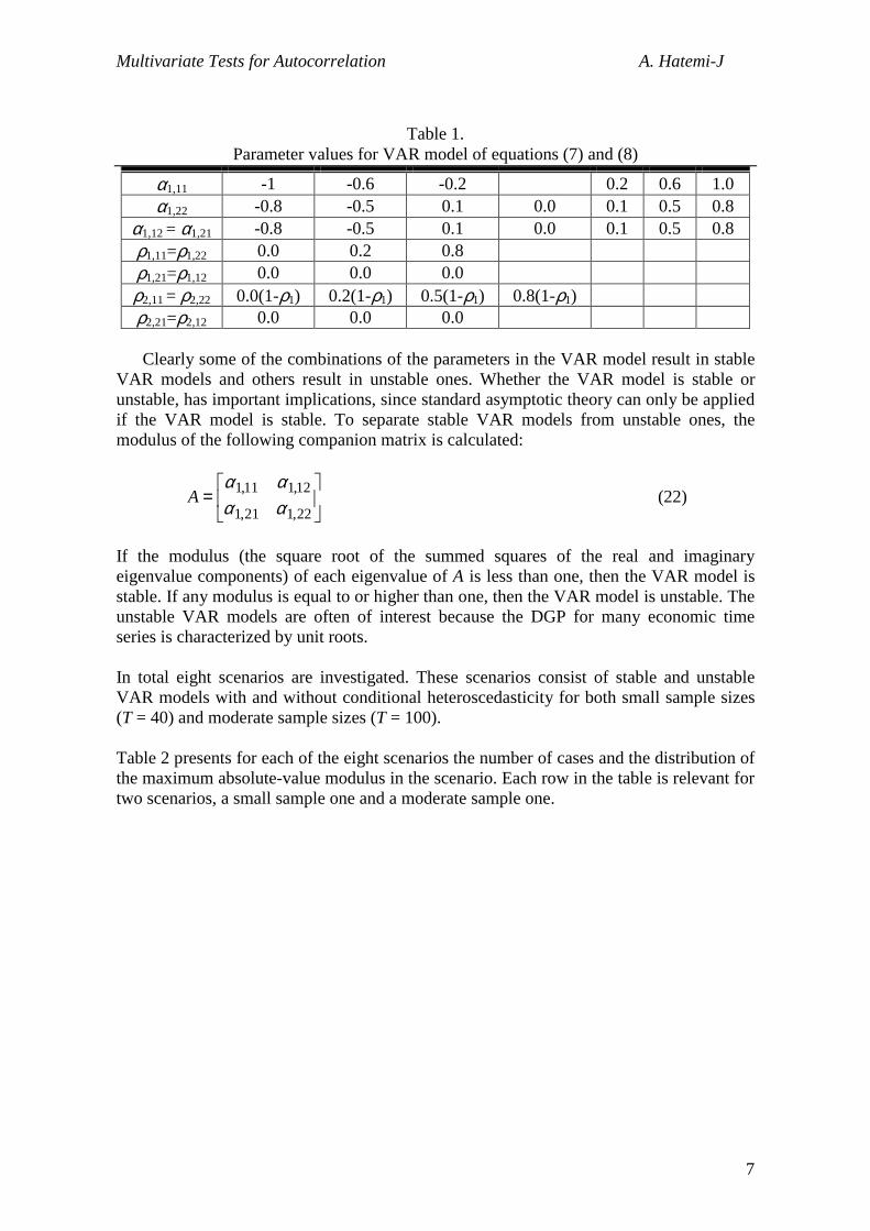
Table 1. Parameter values for VAR model of equations (7) and (8)
α1,11 -1 -0.6 -0.2 0.2 0.6 1.0 α1,22 -0.8 -0.5 0.1 0.0 0.1 0.5 0.8
α1,12 = α1,21 -0.8 -0.5 0.1 0.0 0.1 0.5 0.8 ρ1,11=ρ1,22 0.0 0.2 0.8 ρ1,21=ρ1,12 0.0 0.0 0.0 ρ2,11 = ρ2,22 0.0(1-ρ1) 0.2(1-ρ1) 0.5(1-ρ1) 0.8(1-ρ1) ρ2,21=ρ2,12 0.0 0.0 0.0
Clearly some of the combinations of the parameters in the VAR model result in stable
VAR models and others result in unstable ones. Whether the VAR model is stable or unstable, has important implications, since standard asymptotic theory can only be applied if the VAR model is stable. To separate stable VAR models from unstable ones, the modulus of the following companion matrix is calculated:
=
22,121,1
12,111,1αααα
A (22)
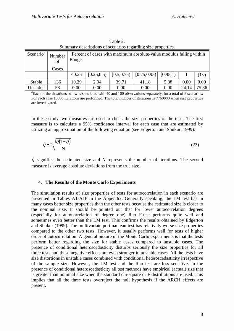
If the modulus (the square root of the summed squares of the real and imaginary eigenvalue components) of each eigenvalue of A is less than one, then the VAR model is stable. If any modulus is equal to or higher than one, then the VAR model is unstable. The unstable VAR models are often of interest because the DGP for many economic time series is characterized by unit roots. In total eight scenarios are investigated. These scenarios consist of stable and unstable VAR models with and without conditional heteroscedasticity for both small sample sizes (T = 40) and moderate sample sizes (T = 100). Table 2 presents for each of the eight scenarios the number of cases and the distribution of the maximum absolute-value modulus in the scenario. Each row in the table is relevant for two scenarios, a small sample one and a moderate sample one.
Multivariate Tests for Autocorrelation A. Hatemi-J
8
Table 2.
Summary descriptions of scenarios regarding size properties. Scenarioa Number
of Cases
Percent of cases with maximum absolute-value modulus falling within Range.
<0.25 [0.25,0.5) [0.5,0.75) [0.75,0.95) [0.95,1) 1 (1≤) Stable 136 10.29 2.94 39.71 41.18 5.88 0.00 0.00
Unstable 58 0.00 0.00 0.00 0.00 0.00 24.14 75.86aEach of the situations below is simulated with 40 and 100 observations separately, for a total of 8 scenarios. For each case 10000 iterations are performed. The total number of iterations is 7760000 when size properties are investigated. In these study two measures are used to check the size properties of the tests. The first measure is to calculate a 95% confidence interval for each case that are estimated by utilizing an approximation of the following equation (see Edgerton and Shukur, 1999):
( )N
ηηη ˆ1ˆ2ˆ −± (23)
η̂ signifies the estimated size and N represents the number of iterations. The second measure is average absolute deviations from the true size.
4. The Results of the Monte Carlo Experiments
The simulation results of size properties of tests for autocorrelation in each scenario are presented in Tables A1-A16 in the Appendix. Generally speaking, the LM test has in many cases better size properties than the other tests because the estimated size is closer to the nominal size. It should be pointed out that for lower autocorrelation degrees (especially for autocorrelation of degree one) Rao F-test performs quite well and sometimes even better than the LM test. This confirms the results obtained by Edgerton and Shukur (1999). The multivariate portmanteau test has relatively worse size properties compared to the other two tests. However, it usually performs well for tests of higher order of autocorrelation. A general picture of the Monte Carlo experiments is that the tests perform better regarding the size for stable cases compared to unstable cases. The presence of conditional heteroscedasticity disturbs seriously the size properties for all three tests and these negative effects are even stronger in unstable cases. All the tests have size distortions in unstable cases combined with conditional heteroscedasticity irrespective of the sample size. However, the LM test and the Rao test are less sensitive. In the presence of conditional heteroscedasticity all test methods have empirical (actual) size that is greater than nominal size when the standard chi-square or F distributions are used. This implies that all the three tests overreject the null hypothesis if the ARCH effects are present.

Multivariate Tests for Autocorrelation A. Hatemi-J
9
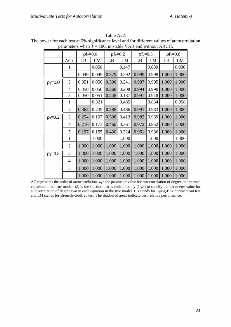
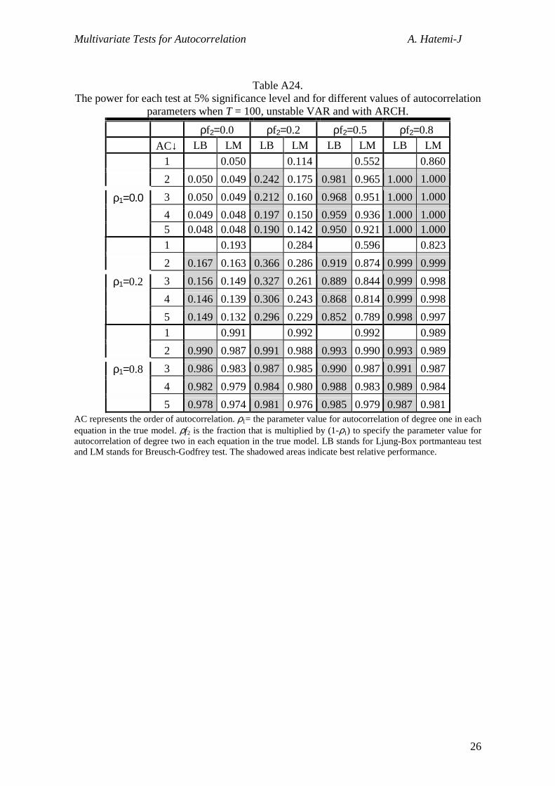
Regarding the power properties of the tests the following can be observed. The LM test and the Rao test have identical power properties so here we concentrate on the power properties of only LM test compared to the portmanteau test. The simulation results for power are presented in Tables A17-A24 in the Appendix. It should be pointed out that the size properties are more important than the power properties. If a test has correct size properties then it is interesting to discover its power properties. If two tests have the same size properties then the one with the higher power should be applied. However, in this study we present the power properties for the portmanteau test also, despite size distortions in many cases. Generally speaking, the power of the tests increases with respect to the order of autocorrelation. Instability results in increasing the power enormously regardless of the sample size. There seems also to be a positive effect from conditional heteroscedasticity on the power properties of the tests. The power of the tests tends to be positively related to the values of the parameters. Generally speaking, the higher the value of the parameters of autocorrelation the higher is the power. When comparing the power of the LM test with portmanteau test it can be concluded that the portmanteau test has usually higher power than the LM test. However, in most cases the difference between the powers of the two tests is rather low.
5. Conclusions
The purpose of this simulation study is to investigate the size and power of three multiviariatrate tests for autocorrelation in the stable and unstable VAR models — namely Ljung-Box portmanteau test, Breusch-Godfrey LM test and Rao F-test — under circumstances of homoscedasticity and autoregressive conditional heteroscedasticity (ARCH). Simulations are conducted for both small sample sizes (T = 40) and moderate sample sizes (T = 100). In total eight scenarios are dealt with.
Regarding the size properties two measures are used. The first measure is a 95%
confidence interval. If the nominal size is within the 95% confidence interval of the empirical size then it is in the acceptance range. The acceptance (or reasonable) rates for all three tests are calculated in each scenario. Since many combinations of the parameters are used in each scenario the results are presented on average. Three different sizes are considered here, i.e. 1% 5% and 10% significance levels. It should be pointed out that the size properties of the tests are investigated when the order of autocorrelation is one to five. Another measure that is used to compare the size performance of the tests is the average absolute deviation of the empirical size from the nominal size. Naturally, the lower the average absolute deviation is the more correct the size. Based on the Monte Carlo experiments one can conclude that all three tests perform quite well in stable VAR models without ARCH. In unstable VAR models portmanteau test has serious size distortions. LM and Rao tests perform very well in unstable VAR models without ARCH. These results are true irrespective of the sample sizes. Another clear result that the simulations show is that none of the tests have correct size when ARCH is present irrespective of VAR models being stable or unstable and regardless of the sample sizes.

Multivariate Tests for Autocorrelation A. Hatemi-J
10
The power properties for each test were also investigated. It should be noted that the power properties of Rao test are the same as LM test. Here we present the power properties of the LM test and the portmanteau test for the sake of comparison. The power for each test is calculated using the five percent significance level. The overall results show that the portmanteau test has better power properties than the LM test. However, the difference in power is usually not significantly large. Since the LM test has better size properties it should be the test that should be used in applied research. However, since this test (as well as the other alternative tests) is sensitive to ARCH effects, it is important to test for ARCH effects before conducting tests for autocorrelation. If the conducted tests show that ARCH effects are present then one possible remedy is to standardize the error terms before tests for autocorrelation are conducted. The estimation of the LM test seems to be easier compared to the Rao test, which makes the LM test the preferred one even though in many cases Rao has as good size properties as LM (and sometimes it is even better, especially for test of lower orders of autocorrelation). The portmanteau test has serious size distortions in unstable VAR models irrespective of having ARCH effects or not. One possible way to improve on the size properties for this test could be making use of the bootstrap simulation techniques. It should be mentioned that the same qualitative results are obtained when the dimension of the VAR model is increased to the case of three variables. The simulation results of the three dimensional VAR model are not presented here to save space but they are available on request.

Multivariate Tests for Autocorrelation A. Hatemi-J
11
Appendix Tables
Table A1. The percentage that is in a 95% confidence interval for actual size for each test when T = 40,
stable VAR models without ARCH. Test ↓
Autocorrelation order →
1 2 3 4 5
The percentage that is in a 95% confidence interval for actual 1% size for each test.
LB 0.765 0.919 0.949 0.978 LM 0.993 1.000 1.000 1.000 1.000 RAO 0.993 1.000 1.000 1.000 0.993 The percentage that is in a 95% confidence interval for actual 5% size for
each test. LB 0.301 0.691 0.794 0.809 LM 0.985 1.000 1.000 0.963 0.934 RAO 0.985 1.000 0.985 0.897 0.529 The percentage that is in a 95% confidence interval for actual 10% size for
each test. LB 0.037 0.544 0.721 0.824 LM 1.000 1.000 0.993 0.978 0.838 RAO 1.000 1.000 0.978 0.868 0.360
LB signifies Ljung-Box portmanteau test, LM stands for Breusch-Godfrey test and RAO represents Rao’s multivariate F-test. The shadowed areas indicate best relative performance.
Table A2. The average absolute deviation from the nominal size when T = 40, stable VAR models without
ARCH. Test ↓
Autocorrelation order →
1 2 3 4 5
The average absolute deviation from the nominal 1% size for each test. LB 0.004 0.003 0.003 0.002 LM 0.001 0.001 0.001 0.001 0.002 RAO 0.001 0.001 0.001 0.002 0.003 The average absolute deviation from the nominal 5% size for each test
when. LB 0.027 0.009 0.007 0.007 LM 0.003 0.002 0.004 0.005 0.006 RAO 0.003 0.002 0.004 0.007 0.010 The average absolute deviation from the nominal 10% size for each test. LB 0.059 0.021 0.012 0.010 LM 0.004 0.004 0.006 0.007 0.011 RAO 0.004 0.004 0.007 0.010 0.016
LB signifies Ljung-Box portmanteau test, LM stands for Breusch-Godfrey test and RAO represents Rao’s multivariate F-test. The shadowed areas indicate best relative performance.
Multivariate Tests for Autocorrelation A. Hatemi-J
12
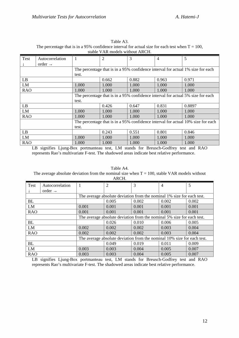
Table A3.
The percentage that is in a 95% confidence interval for actual size for each test when T = 100, stable VAR models without ARCH.
Test ↓
Autocorrelation order →
1 2 3 4 5
The percentage that is in a 95% confidence interval for actual 1% size for each test.
LB 0.662 0.882 0.963 0.971 LM 1.000 1.000 1.000 1.000 1.000 RAO 1.000 1.000 1.000 1.000 1.000 The percentage that is in a 95% confidence interval for actual 5% size for each
test. LB 0.426 0.647 0.831 0.8897 LM 1.000 1.000 1.000 1.000 1.000 RAO 1.000 1.000 1.000 1.000 1.000 The percentage that is in a 95% confidence interval for actual 10% size for each
test. LB 0.243 0.551 0.801 0.846 LM 1.000 1.000 1.000 1.000 1.000 RAO 1.000 1.000 1.000 1.000 1.000
LB signifies Ljung-Box portmanteau test, LM stands for Breusch-Godfrey test and RAO represents Rao’s multivariate F-test. The shadowed areas indicate best relative performance.
Table A4. The average absolute deviation from the nominal size when T = 100, stable VAR models without
ARCH. Test ↓
Autocorrelation order →
1 2 3 4 5
The average absolute deviation from the nominal 1% size for each test. BL 0.005 0.002 0.002 0.002 LM 0.001 0.001 0.001 0.001 0.001 RAO 0.001 0.001 0.001 0.001 0.001 The average absolute deviation from the nominal 5% size for each test. BL 0.026 0.010 0.006 0.005 LM 0.002 0.002 0.002 0.003 0.004 RAO 0.002 0.002 0.002 0.003 0.004 The average absolute deviation from the nominal 10% size for each test. BL 0.049 0.019 0.011 0.009 LM 0.003 0.003 0.004 0.005 0.007 RAO 0.003 0.003 0.004 0.005 0.007
LB signifies Ljung-Box portmanteau test, LM stands for Breusch-Godfrey test and RAO represents Rao’s multivariate F-test. The shadowed areas indicate best relative performance.
Multivariate Tests for Autocorrelation A. Hatemi-J
13
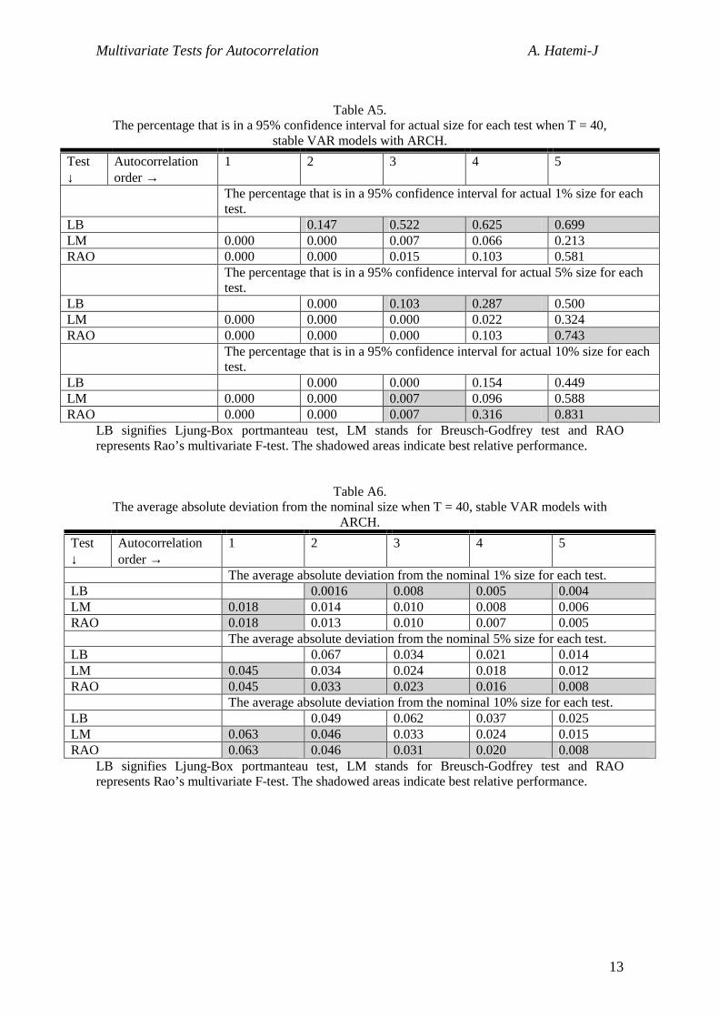
Table A5. The percentage that is in a 95% confidence interval for actual size for each test when T = 40,
stable VAR models with ARCH. Test ↓
Autocorrelation order →
1 2 3 4 5
The percentage that is in a 95% confidence interval for actual 1% size for each test.
LB 0.147 0.522 0.625 0.699 LM 0.000 0.000 0.007 0.066 0.213 RAO 0.000 0.000 0.015 0.103 0.581 The percentage that is in a 95% confidence interval for actual 5% size for each
test. LB 0.000 0.103 0.287 0.500 LM 0.000 0.000 0.000 0.022 0.324 RAO 0.000 0.000 0.000 0.103 0.743 The percentage that is in a 95% confidence interval for actual 10% size for each
test. LB 0.000 0.000 0.154 0.449 LM 0.000 0.000 0.007 0.096 0.588 RAO 0.000 0.000 0.007 0.316 0.831
LB signifies Ljung-Box portmanteau test, LM stands for Breusch-Godfrey test and RAO represents Rao’s multivariate F-test. The shadowed areas indicate best relative performance.
Table A6. The average absolute deviation from the nominal size when T = 40, stable VAR models with
ARCH. Test ↓
Autocorrelation order →
1 2 3 4 5
The average absolute deviation from the nominal 1% size for each test. LB 0.0016 0.008 0.005 0.004 LM 0.018 0.014 0.010 0.008 0.006 RAO 0.018 0.013 0.010 0.007 0.005 The average absolute deviation from the nominal 5% size for each test. LB 0.067 0.034 0.021 0.014 LM 0.045 0.034 0.024 0.018 0.012 RAO 0.045 0.033 0.023 0.016 0.008 The average absolute deviation from the nominal 10% size for each test. LB 0.049 0.062 0.037 0.025 LM 0.063 0.046 0.033 0.024 0.015 RAO 0.063 0.046 0.031 0.020 0.008
LB signifies Ljung-Box portmanteau test, LM stands for Breusch-Godfrey test and RAO represents Rao’s multivariate F-test. The shadowed areas indicate best relative performance.
Multivariate Tests for Autocorrelation A. Hatemi-J
14
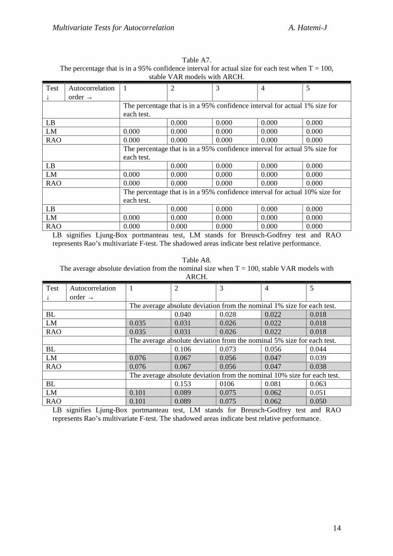
Table A7. The percentage that is in a 95% confidence interval for actual size for each test when T = 100,
stable VAR models with ARCH. Test ↓
Autocorrelation order →
1 2 3 4 5
The percentage that is in a 95% confidence interval for actual 1% size for each test.
LB 0.000 0.000 0.000 0.000 LM 0.000 0.000 0.000 0.000 0.000 RAO 0.000 0.000 0.000 0.000 0.000 The percentage that is in a 95% confidence interval for actual 5% size for
each test. LB 0.000 0.000 0.000 0.000 LM 0.000 0.000 0.000 0.000 0.000 RAO 0.000 0.000 0.000 0.000 0.000 The percentage that is in a 95% confidence interval for actual 10% size for
each test. LB 0.000 0.000 0.000 0.000 LM 0.000 0.000 0.000 0.000 0.000 RAO 0.000 0.000 0.000 0.000 0.000
LB signifies Ljung-Box portmanteau test, LM stands for Breusch-Godfrey test and RAO represents Rao’s multivariate F-test. The shadowed areas indicate best relative performance.
Table A8. The average absolute deviation from the nominal size when T = 100, stable VAR models with
ARCH. Test ↓
Autocorrelation order →
1 2 3 4 5
The average absolute deviation from the nominal 1% size for each test. BL 0.040 0.028 0.022 0.018 LM 0.035 0.031 0.026 0.022 0.018 RAO 0.035 0.031 0.026 0.022 0.018 The average absolute deviation from the nominal 5% size for each test. BL 0.106 0.073 0.056 0.044 LM 0.076 0.067 0.056 0.047 0.039 RAO 0.076 0.067 0.056 0.047 0.038 The average absolute deviation from the nominal 10% size for each test. BL 0.153 0106 0.081 0.063 LM 0.101 0.089 0.075 0.062 0.051 RAO 0.101 0.089 0.075 0.062 0.050
LB signifies Ljung-Box portmanteau test, LM stands for Breusch-Godfrey test and RAO represents Rao’s multivariate F-test. The shadowed areas indicate best relative performance.

Multivariate Tests for Autocorrelation A. Hatemi-J
15
Table A9. The percentage that is in a 95% confidence interval for actual size for each test when T = 40,
unstable VAR models without ARCH. Test
↓ Autocorrelation
order → 1 2 3 4 5
The percentage that is in a 95% confidence interval for actual 1% size for each test.
LB 0.000 0.000 0.000 0.000 LM 1.000 1.000 1.000 1.000 1.000
RAO 1.000 1.000 1.000 1.000 1.000
The percentage that is in a 95% confidence interval for actual 5% size for each test.
LB 0.000 0.000 0.000 0.000 LM 1.000 0.983 0.966 0.966 0.966
RAO 1.000 0.983 0.966 1.000 0.810
The percentage that is in a 95% confidence interval for actual 10% size for each test.
LB 0.000 0.000 0.000 0.000 LM 1.000 0.931 0.983 0.966 0.914
RAO 1.000 0.966 0.983 0.966 0.724 LB signifies Ljung-Box portmanteau test, LM stands for Breusch-Godfrey test and RAO represents Rao’s multivariate F-test. The shadowed areas indicate best relative performance.
Table A10. The average absolute deviation from the nominal size when T = 40, unstable VAR models without
ARCH. Test ↓
Autocorrelation order → 1 2 3 4 5
The average absolute deviation from the nominal 1% size for each test. LB 0.034 0.019 0.015 0.014 LM 0.001 0.001 0.001 0.001 0.001 RAO 0.001 0.001 0.001 0.001 0.002 The average absolute deviation from the nominal 5% size for each test. LB 0.0137 0.008 0.063 0.052 LM 0.002 0.003 0.004 0.004 0.005 RAO 0.002 0.003 0.004 0.004 0.006 The average absolute deviation from the nominal 10% size for each test. LB 0.222 0.138 0.0108 0.090 LM 0.004 0.006 0.007 0.007 0.008 RAO 0.004 0.005 0.007 0.006 0.010
LB signifies Ljung-Box portmanteau test, LM stands for Breusch-Godfrey test and RAO represents Rao’s multivariate F-test. The shadowed areas indicate best relative performance.
Multivariate Tests for Autocorrelation A. Hatemi-J
16
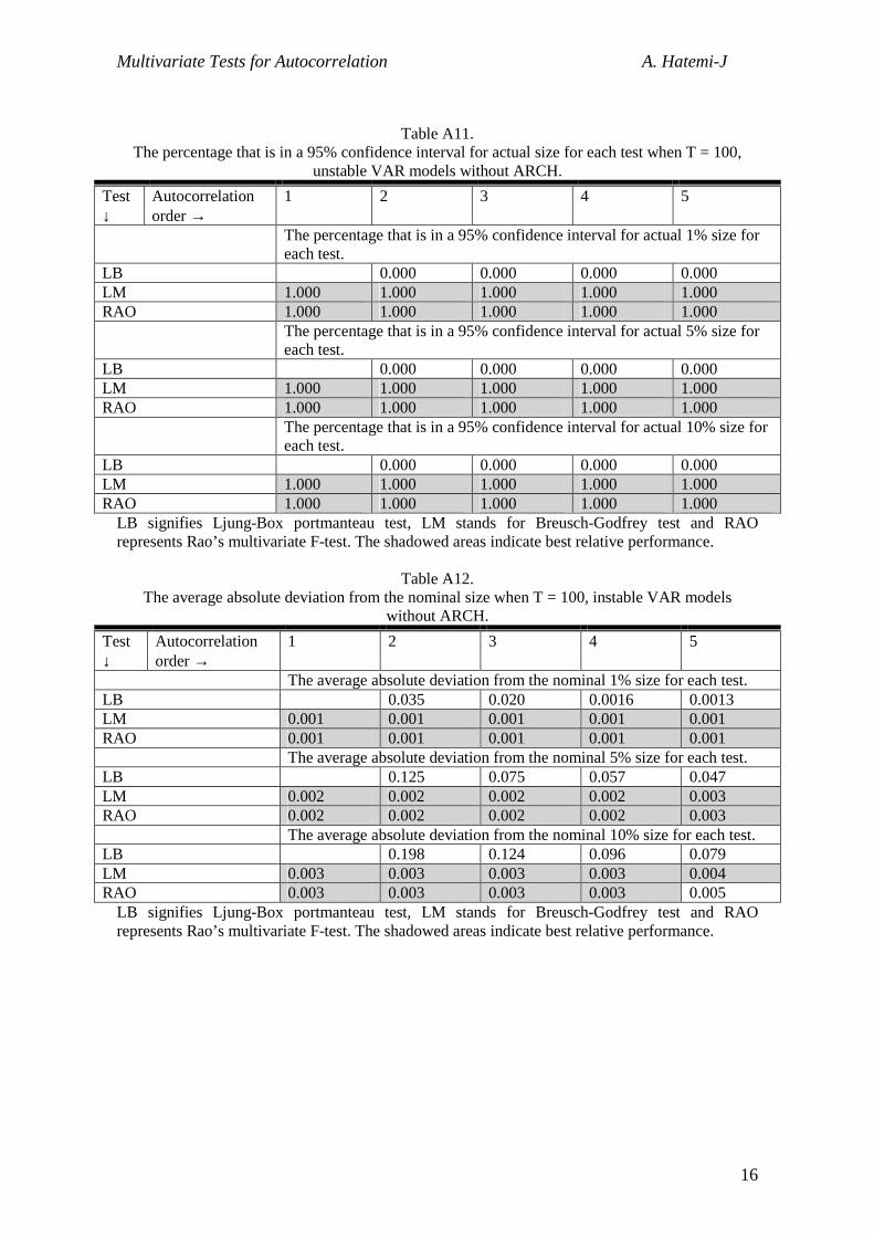
Table A11. The percentage that is in a 95% confidence interval for actual size for each test when T = 100,
unstable VAR models without ARCH. Test ↓
Autocorrelation order →
1 2 3 4 5
The percentage that is in a 95% confidence interval for actual 1% size for each test.
LB 0.000 0.000 0.000 0.000 LM 1.000 1.000 1.000 1.000 1.000 RAO 1.000 1.000 1.000 1.000 1.000 The percentage that is in a 95% confidence interval for actual 5% size for
each test. LB 0.000 0.000 0.000 0.000 LM 1.000 1.000 1.000 1.000 1.000 RAO 1.000 1.000 1.000 1.000 1.000 The percentage that is in a 95% confidence interval for actual 10% size for
each test. LB 0.000 0.000 0.000 0.000 LM 1.000 1.000 1.000 1.000 1.000 RAO 1.000 1.000 1.000 1.000 1.000
LB signifies Ljung-Box portmanteau test, LM stands for Breusch-Godfrey test and RAO represents Rao’s multivariate F-test. The shadowed areas indicate best relative performance.
Table A12. The average absolute deviation from the nominal size when T = 100, instable VAR models
without ARCH. Test ↓
Autocorrelation order →
1 2 3 4 5
The average absolute deviation from the nominal 1% size for each test. LB 0.035 0.020 0.0016 0.0013 LM 0.001 0.001 0.001 0.001 0.001 RAO 0.001 0.001 0.001 0.001 0.001 The average absolute deviation from the nominal 5% size for each test. LB 0.125 0.075 0.057 0.047 LM 0.002 0.002 0.002 0.002 0.003 RAO 0.002 0.002 0.002 0.002 0.003 The average absolute deviation from the nominal 10% size for each test. LB 0.198 0.124 0.096 0.079 LM 0.003 0.003 0.003 0.003 0.004 RAO 0.003 0.003 0.003 0.003 0.005
LB signifies Ljung-Box portmanteau test, LM stands for Breusch-Godfrey test and RAO represents Rao’s multivariate F-test. The shadowed areas indicate best relative performance.

Multivariate Tests for Autocorrelation A. Hatemi-J
17
Table A13. The percentage that is in a 95% confidence interval for actual size for each test when T = 40,
unstable VAR models with ARCH. Test ↓
Autocorrelation order →
1 2 3 4 5
The percentage that is in a 95% confidence interval for actual 1% size for each test.
LB 0.000 0.000 0.000 0.000 LM 0.000 0.000 0.000 0.000 0.000 RAO 0.000 0.000 0.000 0.000 0.000 The percentage that is in a 95% confidence interval for actual 5% size for each
test. LB 0.000 0.000 0.000 0.000 LM 0.000 0.000 0.000 0.000 0.000 RAO 0.000 0.000 0.000 0.000 0.000 The percentage that is in a 95% confidence interval for actual 10% size for each
test. LB 0.000 0.000 0.000 0.000 LM 0.000 0.000 0.000 0.000 0.000 RAO 0.000 0.000 0.000 0.000 0.000
LB signifies Ljung-Box portmanteau test, LM stands for Breusch-Godfrey test and RAO represents Rao’s multivariate F-test. The shadowed areas indicate best relative performance.
Table A14. The average absolute deviation from the nominal size when T = 40, unstable VAR models with
ARCH. Test ↓
Autocorrelation order →
1 2 3 4 5
The average absolute deviation from the nominal 1% size for each test. LB 0.008 0.049 0.038 0.032 LM 0.025 0.022 0.015 0.012 0.009 RAO 0.025 0.021 0.014 0.011 0.007 The average absolute deviation from the nominal 5% size for each test. LB 0.224 0.143 0.110 0.090 LM 0.061 0.055 0.038 0.032 0.023 RAO 0.061 0.054 0.036 0.029 0.018 The average absolute deviation from the nominal 10% size for each test. LB 0.320 0.215 0.167 0.136 LM 0.083 0.077 0.054 0.067 0.033 RAO 0.083 0.076 0.052 0.043 0.026
LB signifies Ljung-Box portmanteau test, LM stands for Breusch-Godfrey test and RAO represents Rao’s multivariate F-test. The shadowed areas indicate best relative performance.

Multivariate Tests for Autocorrelation A. Hatemi-J
18
Table A15. The percentage that is in a 95% confidence interval for actual size for each test when T = 100,
unstable VAR models with ARCH. Test ↓
Autocorrelation order → 1 2 3 4 5
The percentage that is in a 95% confidence interval for actual 1% size for each test.
LB 0.000 0.000 0.000 0.000 LM 0.000 0.000 0.000 0.000 0.000 RAO 0.000 0.000 0.000 0.000 0.000
The percentage that is in a 95% confidence interval for actual 5% size for each test.
LB 0.000 0.000 0.000 0.000 LM 0.000 0.000 0.000 0.000 0.000 RAO 0.000 0.000 0.000 0.000 0.000
The percentage that is in a 95% confidence interval for actual 10% size for each test.
LB 0.000 0.000 0.000 0.000 LM 0.000 0.000 0.000 0.000 0.000 RAO 0.000 0.000 0.000 0.000 0.000
LB signifies Ljung-Box portmanteau test, LM stands for Breusch-Godfrey test and RAO represents Rao’s multivariate F-test. The shadowed areas indicate best relative performance.
Table A16. The average absolute deviation from the nominal size when T = 100, unstable VAR models with
ARCH. Test ↓
Autocorrelation order → 1 2 3 4 5
The average absolute deviation from the nominal 1% size for each test. LB 0.132 0.091 0.072 0.060 LM 0.053 0.049 0.040 0.033 0.027 RAO 0.053 0.049 0.039 0.033 0.026 The average absolute deviation from the nominal 5% size for each test. LB 0.280 0.201 0.161 0.135 LM 0.106 0.102 0.085 0.073 0.060 RAO 0.106 0.102 0.084 0.072 0.059 The average absolute deviation from the nominal 10% size for each test. LB 0.365 0.270 0.220 0.185 LM 0.136 0.133 0.112 0.097 0.080 RAO 0.136 0.133 0.112 0.096 0.079
LB signifies Ljung-Box portmanteau test, LM stands for Breusch-Godfrey test and RAO represents Rao’s multivariate F-test. The shadowed areas indicate best relative performance.

Multivariate Tests for Autocorrelation A. Hatemi-J
19
Table A17. The power for each test at 5% significance level and for different values of autocorrelation
parameters when T = 40, stable VAR and without ARCH. ρf2=0.0 ρf2=0.2 ρf2=0.5 ρf2=0.8 AC↓ LB LM LB LM LB LM LB LM
1 0.050 0.72 0.419 0.857
2 0.050 0.049 0.126 0.080 0.758 0.576 0.994 0.976
ρ1=0.0 3 0.050 0.050 0.092 0.076 0.643 0.498 0.986 0.9614 0.050 0.050 0.086 0.071 0.582 0.433 0.978 0.941 5 0.050 0.050 0.086 0.070 0.550 0.382 0.970 0.919
1 0.086 0.108 0.328 0.697
2 0.071 0.073 0.143 0.101 0.585 0.410 0.947 0.860
ρ1=0.2 3 0.071 0.068 0.107 0.090 0.461 0.348 0.900 0.808
4 0.070 0.046 0.100 0.084 0.411 0.301 0.862 0.755
5 0.069 0.063 0.098 0.079 0.382 0.266 0.834 0.706 1 0.641 0.650 0.668 0.686
2 0.689 0.609 0.713 0.624 0.748 0.648 0.783 0.675
ρ1=0.8 3 0.599 0.558 0.626 0.575 0.668 0.604 0.708 0.632
4 0.557 0.511 0.582 0.529 0.624 0.561 0.665 0.591
5 0.531 0.473 0.554 0.493 0.593 0.527 0.635 0.557AC represents the order of autocorrelation. ρ1= the parameter value for autocorrelation of degree one in each equation in the true model. ρf2 is the fraction that is multiplied by (1-ρ1) to specify the parameter value for autocorrelation of degree two in each equation in the true model. LB stands for Ljung-Box portmanteau test and LM stands for Breusch-Godfrey test. The shadowed areas indicate best relative performance.

Multivariate Tests for Autocorrelation A. Hatemi-J
20
Table A18.
The power for each test at 5% significance level and for different values of autocorrelation parameters when T = 100, stable VAR and without ARCH. .
ρf2=0.0 ρf2=0.2 ρf2=0.5 ρf2=0.8 AC↓ LB LM LB LM LB LM LB LM
1 0.050 0.206 0.879 0.990
2 0.050 0.050 0.411 0.287 0.999 0.995 1.00 1.00
ρ1=0.0 3 0.050 0.051 0.307 0.237 0.997 0.990 1.00 1.00 4 0.050 0.051 0.259 0.208 0.993 0.984 1.00 1.00 5 0.050 0.050 0.234 0.185 0.989 0.975 1.00 1.00
1 0.192 0.339 0.835 0.970
2 0.148 0.147 0.453 0.354 0.984 0.955 1.00 1.00
ρ1=0.2 3 0.130 0.126 0.355 0.298 0.963 0.930 1.00 1.00
4 0.121 0.114 0.312 0.262 0.941 0.904 1.00 1.00
5 0.116 0.104 0.287 0.232 0.921 0.877 1.00 0.999 1 0.879 0.887 0.904 0.924
2 0.899 0.872 0.909 0.880 0.929 0.896 0.952 0.915
ρ1=0.8 3 0.873 0.856 0.886 0.866 0.909 0.884 0.934 0.902
4 0.857 0.842 0.870 0.853 0.894 0.873 0.920 0.892
5 0.844 0.829 0.857 0.841 0.883 0.862 0.910 0.883AC represents the order of autocorrelation. ρ1= the parameter value for autocorrelation of degree one in each equation in the true model. ρf2 is the fraction that is multiplied by (1-ρ1) to specify the parameter value for autocorrelation of degree two in each equation in the true model. LB stands for Ljung-Box portmanteau test and LM stands for Breusch-Godfrey test. The shadowed areas indicate best relative performance.

Multivariate Tests for Autocorrelation A. Hatemi-J
21
Table A19. The power for each test at 5% significance level and for different values of autocorrelation
parameters when T = 40, stable VAR and with ARCH. ρf2=0.0 ρf2=0.2 ρf2=0.5 ρf2=0.8 AC↓ LB LM LB LM LB LM LB LM
1 0.050 0.060 0.288 0.709
2 0.049 0.051 0.101 0.064 0.609 0.401 0.970 0.908
ρ1=0.0 3 0.050 0.050 0.077 0.064 0.501 0.354 0.947 0.8794 0.049 0.050 0.073 0.062 0.543 0.314 0.928 0.847 5 0.050 0.050 0.088 0.063 0.429 0.285 0.911 0.815
1 0.075 0.082 0.208 0.514
2 0.067 0.068 0.073 0.079 0.428 0.263 0.857 0.699
ρ1=0.2 3 0.067 0.065 0.111 0.075 0.331 0.234 0.784 0.646
4 0.067 0.062 0.086 0.072 0.297 0.211 0.740 0.598
5 0.066 0.061 0.082 0.070 0.280 0.192 0.708 0.556 1 0.485 0.485 0.492 0.509
2 0.506 0.442 0.524 0.446 0.558 0.465 0.597 0.493
ρ1=0.8 3 0.431 0.403 0.446 0.410 0.477 0.431 0.520 0.463
4 0.398 0.367 0.412 0.377 0.441 0.401 0.484 0.435
5 0.381 0.340 0.393 0.353 0.417 0.377 0.454 0.413AC represents the order of autocorrelation. ρ1= the parameter value for autocorrelation of degree one in each equation in the true model. ρf2 is the fraction that is multiplied by (1-ρ1) to specify the parameter value for autocorrelation of degree two in each equation in the true model. LB stands for Ljung-Box portmanteau test and LM stands for Breusch-Godfrey test. The shadowed areas indicate best relative performance.
Multivariate Tests for Autocorrelation A. Hatemi-J
22
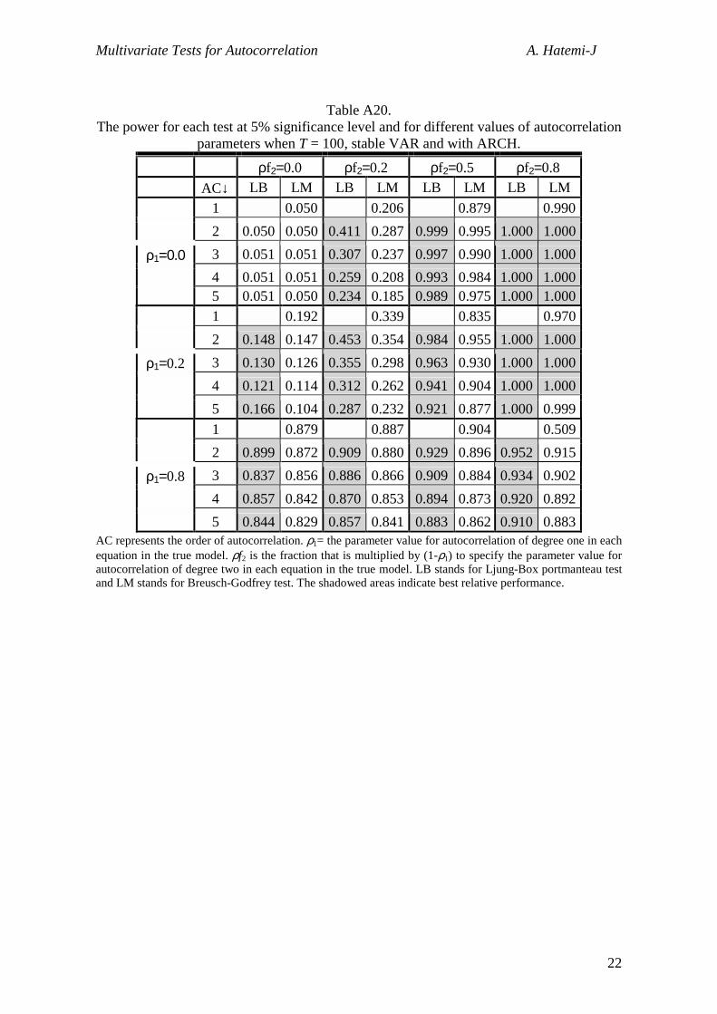
Table A20. The power for each test at 5% significance level and for different values of autocorrelation
parameters when T = 100, stable VAR and with ARCH. ρf2=0.0 ρf2=0.2 ρf2=0.5 ρf2=0.8 AC↓ LB LM LB LM LB LM LB LM
1 0.050 0.206 0.879 0.990
2 0.050 0.050 0.411 0.287 0.999 0.995 1.000 1.000
ρ1=0.0 3 0.051 0.051 0.307 0.237 0.997 0.990 1.000 1.0004 0.051 0.051 0.259 0.208 0.993 0.984 1.000 1.000 5 0.051 0.050 0.234 0.185 0.989 0.975 1.000 1.000
1 0.192 0.339 0.835 0.970
2 0.148 0.147 0.453 0.354 0.984 0.955 1.000 1.000
ρ1=0.2 3 0.130 0.126 0.355 0.298 0.963 0.930 1.000 1.000
4 0.121 0.114 0.312 0.262 0.941 0.904 1.000 1.000
5 0.166 0.104 0.287 0.232 0.921 0.877 1.000 0.999 1 0.879 0.887 0.904 0.509
2 0.899 0.872 0.909 0.880 0.929 0.896 0.952 0.915
ρ1=0.8 3 0.837 0.856 0.886 0.866 0.909 0.884 0.934 0.902
4 0.857 0.842 0.870 0.853 0.894 0.873 0.920 0.892
5 0.844 0.829 0.857 0.841 0.883 0.862 0.910 0.883AC represents the order of autocorrelation. ρ1= the parameter value for autocorrelation of degree one in each equation in the true model. ρf2 is the fraction that is multiplied by (1-ρ1) to specify the parameter value for autocorrelation of degree two in each equation in the true model. LB stands for Ljung-Box portmanteau test and LM stands for Breusch-Godfrey test. The shadowed areas indicate best relative performance.

Multivariate Tests for Autocorrelation A. Hatemi-J
23
Table A21. The power for each test at 5% significance level and for different values of autocorrelation
parameters when T = 40, unstable VAR and without ARCH. ρf2=0.0 ρf2=0.2 ρf2=0.5 ρf2=0.8 AC↓ LB LM LB LM LB LM LB LM
1 0.050 0.082 0.339 0.761
2 0.050 0.050 0.119 0.077 0.713 0.576 0.991 0.980
ρ1=0.0 3 0.050 0.050 0.105 0.073 0.634 0.498 0.983 0.9654 0.051 0.050 0.098 0.069 0.590 0.426 0.976 0.945 5 0.050 0.050 0.098 0.068 0.566 0.381 0.969 0.923
1 0.108 0.149 0.341 0.628
2 0.091 0.087 0.168 0.114 0.568 0.430 0.928 0.871
ρ1=0.2 3 0.089 0.078 0.142 0.103 0.490 0.370 0.885 0.820
4 0.089 0.073 0.134 0.092 0.448 0.316 0.8856 0.764
5 0.088 0.070 0.131 0.086 0.428 0.282 0.835 0.717 1 0.958 0.960 0.962 0.962
2 0.942 0.924 0.948 0.928 0.958 0.937 0.963 0.939
ρ1=0.8 3 0.906 0.889 0.916 0.898 0.933 0.911 0.940 0.916
4 0.880 0.849 0.894 0.863 0.914 0.880 0.923 0.889
5 0.863 0.816 0.879 0.831 0.901 0.855 0.910 0.868AC represents the order of autocorrelation. ρ1= the parameter value for autocorrelation of degree one in each equation in the true model. ρf2 is the fraction that is multiplied by (1-ρ1) to specify the parameter value for autocorrelation of degree two in each equation in the true model. LB stands for Ljung-Box portmanteau test and LM stands for Breusch-Godfrey test. The shadowed areas indicate best relative performance.
Multivariate Tests for Autocorrelation A. Hatemi-J
24
Table A22. The power for each test at 5% significance level and for different values of autocorrelation
parameters when T = 100, unstable VAR and without ARCH. ρf2=0.0 ρf2=0.2 ρf2=0.5 ρf2=0.8 AC↓ LB LM LB LM LB LM LB LM
1 0.050 0.147 0.689 0.938
2 0.049 0.049 0.379 0.292 0.999 0.998 1.000 1.000
ρ1=0.0 3 0.051 0.050 0.306 0.241 0.997 0.995 1.000 1.0004 0.050 0.050 0.268 0.208 0.994 0.990 1.000 1.000 5 0.050 0.051 0.248 0.187 0.991 0.948 1.000 1.000
1 0.321 0.485 0.834 0.958
2 0.362 0.239 0.588 0.486 0.991 0.983 1.000 1.000
ρ1=0.2 3 0.254 0.197 0.508 0.413 0.982 0.969 1.000 1.000
4 0.216 0.173 0.460 0.361 0.972 0.952 1.000 1.000
5 0.197 0.155 0.430 0.324 0.961 0.936 1.000 1.000 1 1.000 1.000 1.000 1.000
2 1.000 1.000 1.000 1.000 1.000 1.000 1.000 1.000
ρ1=0.8 3 1.000 1.000 1.000 1.000 1.000 1.000 1.000 1.000
4 1.000 1.000 1.000 1.000 1.000 1.000 1.000 1.000
5 1.000 1.000 1.000 1.000 1.000 1.000 1.000 1.000
1.000 1.000 1.000 1.000 1.000 1.000 1.000 1.000AC represents the order of autocorrelation. ρ1= the parameter value for autocorrelation of degree one in each equation in the true model. ρf2 is the fraction that is multiplied by (1-ρ1) to specify the parameter value for autocorrelation of degree two in each equation in the true model. LB stands for Ljung-Box portmanteau test and LM stands for Breusch-Godfrey test. The shadowed areas indicate best relative performance.

Multivariate Tests for Autocorrelation A. Hatemi-J
25
Table A23. The power for each test at 5% significance level and for different values of autocorrelation
parameters when T = 40, unstable VAR and with ARCH. ρf2=0.0 ρf2=0.2 ρf2=0.5 ρf2=0.8 AC↓ LB LM LB LM LB LM LB LM
1 0.051 0.076 0.243 0.590
2 0.049 0.050 0.106 0.066 0.540 0.388 0.953 0.910
ρ1=0.0 3 0.050 0.050 0.097 0.067 0.490 0.353 0.929 0.8854 0.049 0.049 0.090 0.065 0.458 0.315 0.918 0.853 5 0.050 0.048 0.088 0.063 0.447 0.288 0.905 0.824
1 0.089 0.110 0.217 0.416
2 0.080 0.079 0.130 0.089 0.395 0.267 0.799 0.688
ρ1=0.2 3 0.080 0.075 0.115 0.086 0.349 0.245 0.745 0.642
4 0.079 0.071 0.109 0.082 0.324 0.222 0.714 0.593
5 0.079 0.068 0.109 0.079 0.315 0.206 0.695 0.552 1 0.641 0.770 0.773 0.764
2 0.737 0.700 0.748 0.697 0.769 0.703 0.778 0.704
ρ1=0.8 3 0.678 0.649 0.687 0.648 0.711 0.659 0.728 0.665
4 0.644 0.601 0.654 0.600 0.675 0.615 0.691 0.624
5 0.625 0.560 0.636 0.563 0.653 0.578 0.666 0.593AC represents the order of autocorrelation. ρ1= the parameter value for autocorrelation of degree one in each equation in the true model. ρf2 is the fraction that is multiplied by (1-ρ1) to specify the parameter value for autocorrelation of degree two in each equation in the true model. LB stands for Ljung-Box portmanteau test and LM stands for Breusch-Godfrey test. The shadowed areas indicate best relative performance.
Multivariate Tests for Autocorrelation A. Hatemi-J
26
Table A24. The power for each test at 5% significance level and for different values of autocorrelation
parameters when T = 100, unstable VAR and with ARCH. ρf2=0.0 ρf2=0.2 ρf2=0.5 ρf2=0.8 AC↓ LB LM LB LM LB LM LB LM
1 0.050 0.114 0.552 0.860
2 0.050 0.049 0.242 0.175 0.981 0.965 1.000 1.000
ρ1=0.0 3 0.050 0.049 0.212 0.160 0.968 0.951 1.000 1.0004 0.049 0.048 0.197 0.150 0.959 0.936 1.000 1.000 5 0.048 0.048 0.190 0.142 0.950 0.921 1.000 1.000
1 0.193 0.284 0.596 0.823
2 0.167 0.163 0.366 0.286 0.919 0.874 0.999 0.999
ρ1=0.2 3 0.156 0.149 0.327 0.261 0.889 0.844 0.999 0.998
4 0.146 0.139 0.306 0.243 0.868 0.814 0.999 0.998
5 0.149 0.132 0.296 0.229 0.852 0.789 0.998 0.997 1 0.991 0.992 0.992 0.989
2 0.990 0.987 0.991 0.988 0.993 0.990 0.993 0.989
ρ1=0.8 3 0.986 0.983 0.987 0.985 0.990 0.987 0.991 0.987
4 0.982 0.979 0.984 0.980 0.988 0.983 0.989 0.984
5 0.978 0.974 0.981 0.976 0.985 0.979 0.987 0.981AC represents the order of autocorrelation. ρ1= the parameter value for autocorrelation of degree one in each equation in the true model. ρf2 is the fraction that is multiplied by (1-ρ1) to specify the parameter value for autocorrelation of degree two in each equation in the true model. LB stands for Ljung-Box portmanteau test and LM stands for Breusch-Godfrey test. The shadowed areas indicate best relative performance.

Multivariate Tests for Autocorrelation A. Hatemi-J
27
References
Anderson T. W. (1958), “An Introduction to Multivariate Statistical Analysis,” New York, Wily.
Box G. E. P. and Pierce D. A., (1970), “Distribution of Residual Autocorrelation in Autoregressive Moving Average Time Series Models,” Journal of the American Statistical Association, 65, 1509-1526.
Breusch T. S. (1978), “Testing for Autocorrelation in Dynamic Linear Models,” Australian Economic Papers, 17, 334-355.
Durbin J. (1970) “Testing for Serial Correlation Least Squares Regression When Some of the Regressors are Lagged Dependent Variables”, Econometrica, 38, 410-421.
Durbin J, and Watson G, (1950) “Testing for Serial Correlation in Least Squares Regression”, Biometrika, 37, 409-428.
Edgerton, D. and Shukur, G., (1999) “Testing Autocorrelation in a System Perspective” Econometric Reviews, 18(4), 343-86.
Engle, R. F (1982) “Autoregressive Conditional Heteroscedasticity with Estimates of the Variance of United Kingdom Inflation” Econometrica, 50(4), 987-1007.
Godfrey L. G. (1978), “Testing for Higher Order Serial Correlation in Regression Equations When the Regressors Include Lagged Dependent Variables,” Econometrica, 46, 1303-1310.
Greene W. H. (2001), “Econometric Analysis,” Fourth Edition, Prentice Hall. Hatemi-J A. (2002) “A New Method to Choose the Optimal Lag Order in Stable and
Unstable VAR Models. Applied Economics Letters, forthcoming. Hendry and Mizon. (1999) Hosking J R M (1980) “The Multivariate Portmanteau Statistic” Journal of American
Statistical Association, 75, 602-608. Johansen, S. (1996) “Likelihood Based Inference in Cointegrated Vector
Autoregressive Models”. Advanced Texts in Econometrics, Oxford University Press. Ljung G. M. and Box G. E. P. (1978), “On a Measure of Lack of Fit in Time-Series
Models,” Biometrika, 66, 265-270. Rao, C. R. (1973) “Linear Statistical Inference and Its Application,” Second edition.
New York: Wiley.