Multivariate survival analysis with doubly-censored data: application to the assessment of Accutane...

STATISTICS IN MEDICINEStatist. Med. 2002; 21:2547–2562 (DOI: 10.1002/sim.1123)

Multivariate survival analysis with doubly-censored data:application to the assessment of Accutane treatment for

�brodysplasia ossi�cans progressiva

Geo�rey Jones1 and David M. Rocke2;∗;†

1Department of Statistics; Massey University; Palmerston North; New Zealand2Department of Applied Science; University of California; Davis CA 95616; U.S.A.

SUMMARY

Fibrodysplasia ossi�cans progressiva is a rare genetic disorder in which the joints of patients becomedisabled by the formation of heterotopic bone. Data are available on the status of 11 joints of each of21 patients before, during and after treatment with Accutane. These are compared with data obtainedby questionnaire from 40 untreated patients to determine the e�cacy of the treatment. Both left- andright-censoring are present in each group, which, together with the multivariate nature of the data andthe time-dependent treatment covariate, makes analysis di�cult. We consider two alternative parametricmodels for incorporating within-subject dependence: a marginal model and a frailty model. Both analysessuggest that Accutane treatment is e�ective. We discuss and illustrate the di�erences between the twoapproaches. We also discuss the extent to which the conclusions are compromised by the observationalnature of the study. Copyright ? 2002 John Wiley & Sons, Ltd.

1. INTRODUCTION

Fibrodysplasia ossi�cans progressiva (FOP) is an extremely rare and disabling genetic dis-order characterized by progressive heterotopic ossi�cation of soft tissues, leading to the im-mobilization of a�ected joints. Bone formation can be stimulated by blunt trauma, surgery,intramuscular injection or aggressive physical therapy, but most often occurs spontaneously.At present no e�ective prevention or treatment is known [1].In 1992, 44 patient members of the International Fibrodysplasia Ossi�cans Progressiva

Association responded to a postal survey of the age at onset of heterotopic ossi�cation ateach of 15 anatomic sites [2]. For each patient in the survey, and for each anatomic site,the patient was asked to record the date at onset of heterotopic ossi�cation. Right-censoringoccurred when a particular joint was uninvolved at the time of the survey: left-censoring

∗Correspondence to: David M. Rocke, Center for Image Processing and Integrated Computing, Department ofApplied Science, One Shields Avenue, University of California, Davis, CA 95616-8553, U.S.A.

†E-mail: [email protected]=grant sponsor: NSF; contract=grant numbers: AC1 96-19020, DMS 98-70172, DMS 95-10511

Received September 1999Copyright ? 2002 John Wiley & Sons, Ltd. Accepted August 2001

2548 G. JONES AND D. M. ROCKE

when the patient replied that a joint was already involved but they could not provide thedate of onset. From the 660 onset times in the survey, 231 were right-censored and 41left-censored.Retinoids are a plausible family of therapeutic agents for FOP because of their ability to

inhibit di�erentiation of mesenchymal tissue into cartilage and bone. An age-matched internalcontrol study was designed to determine the e�ectiveness of 13-cis-retinoic acid (Accutane)in the prevention of new heterotopic lesions in patients. After nearly one year of attemptedrecruitment, it proved impossible to assemble an internal age- and disease-severity-matchedcontrol group. Most patients over 21 had severe symptoms and did not wish to receiveAccutane, whereas most under 21 had more mild manifestations of FOP and were unwillingto receive a placebo. Because of this, and the extreme rarity of the condition, it was decidedto recruit FOP patients into a treatment group only and to use the survey data as an externalcontrol.Twenty-one patients who had FOP were recruited sequentially during an initial or follow-

up visit to the FOP clinic at the National Institute of Health. Eleven anatomic regions wereassessed in each of the 21 patients by clinical examination, plain roentgenograms and radionu-clide bone scans. An anatomic region was considered to be involved if there was clinical,roentgenographic or radionuclide evidence of orthotopic or heterotopic ossi�cation anywherein that region. The regions thus assessed in the treatment group were the neck, spine, jaw,right shoulder, left shoulder, right elbow, left elbow, right hip, left hip, right knee and leftknee; these regions were also included in the survey data from the external control, along withright=left wrist and ankle. The duration of treatment ranged from four months to ten years,with median three years and quartiles one and �ve years. The total number of uninvolvedjoints prior to treatment was 88; only two of these became involved during treatment, bothbelonging to the same patient.There are a number of problems in assessing the e�ectiveness of the treatment. The lack

of an internal control group may lead to bias, especially since the selection criterion and thecriterion for diagnosis of involvement of an anatomic region is di�erent in each group. Wepostpone discussion of this point until Section 5, where possible group di�erences are analysed.Our main focus of consideration is the multivariate nature of the data. The total number ofpatients is too small for the e�ect of treatment on any single uninvolved joint to be estimatedwith any precision, so it is necessary to examine all anatomic regions simultaneously and tosomehow account for the within-patient dependence. Thus the data are highly multivariate,with 11 observations on each subject corresponding to the status of each of 11 anatomicalsites. The presence of both left- and right-censoring, and a time-dependent covariate, increasethe technical di�culty of analysis.There is now a large literature on multivariate survival analysis. The marginal model ap-

proach of Wei et al. [3] �ts univariate models to the marginal distributions and uses Huber’ssandwich estimator [4] to make joint inference about the regression parameters from eachmodel, with no attempt made to model the within-patient dependence. The frailty model ap-proach, on the other hand, attempts a parametric model of this dependence by postulatinga patient-speci�c parameter, a ‘frailty’, to account for each patient’s particular susceptibilityto new events [5–8]. It is usual in both approaches to assume proportional hazards and tomodel the baseline hazard functions non-parametrically, as in the Cox model, although theinterpretation of proportionality varies, applying to the marginals in the �rst approach andthe conditional distributions given the frailty in the second. Parametric models for the hazard

Copyright ? 2002 John Wiley & Sons, Ltd. Statist. Med. 2002; 21:2547–2562

MULTIVARIATE SURVIVAL ANALYSIS WITH DOUBLY-CENSORED DATA 2549

functions are also possible. Huster et al. [9] explicitly compared the two approaches in a para-metric analysis of paired survival data, �nding that the marginal approach was computationallysimpler but less e�cient.The commonly used partial likelihood approach cannot be used for our data because of the

double censoring. Several authors [10–12] have examined the estimation of semi-parametricproportional hazard models with doubly-censored or interval-censored data, but time-dependentcovariates seem to present a special challenge in this context. Recent work by Goggins et al.[13] applies the Cox model for an interval-censored time-dependent covariate to data which isexact or right-censored. We have attempted to solve the combination of di�culties in the FOPdata by using parametric versions of both a marginal model and a frailty model, which wethen compare. The advantage of a parametric approach here is the relative ease of handlingof di�erent censoring patterns. Although our data contained no interval-censoring the methodsare easily extended to cover such cases.In applications the multiple events are either homogeneous (same hazard structure) or het-

erogeneous. Our data set arguably has both types: some joints, such as the neck and jaw,clearly have di�erent baseline hazards whereas pairs such as right knee=left knee might beexpected to be the same. An additional complication is the small number of patient-years ontreatment, which together with the few observed failures during treatment makes a straight-forward application of the robust variance in the marginal model invalid. We propose atransformation which improves the performance of this method in such circumstances.The paper is organized as follows. We �rst discuss the modelling of the marginal distri-

butions, then in Section 3 investigate inference for the treatment e�ect using this marginalmodel. In Section 4 we develop a frailty model and discuss its estimation. Possible groupdi�erences are investigated in Section 5 using both approaches. Finally, in Section 6 we com-pare two approaches and discuss their implications for the use of Accutane in treating FOP.Some of the statistical results from this paper were used in Zaslo� et al. [14].

2. THE MARGINAL MODEL

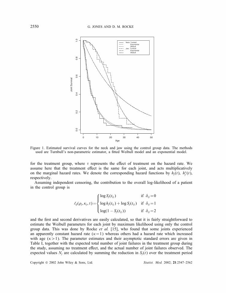
Here we consider modelling the age Tij of the ith patient at the onset of involvement ofjoint j. Ignoring for the moment the treatment e�ect and any other covariates, we observe(tij; �ij); i=1; : : : ; n where �=0 indicates right-censoring (in which case Tij¿tij); �=1 foruncensored observations (Tij= tij) and �=2 for left-censoring (Tij¡tij). Rocke et al. [15]examined the marginal distributions for the control group using both Weibull models andTurnbull’s non-parametric estimator [16]. Examples of the resulting survival curves, from thecontrol group survey data, are given in Figure 1. The Weibull model gives results similar tothe Turnbull estimates, and is more attractive since it can handle the time-dependent treatmentcovariate relatively easily.Adopting the Weibull model, we assume that Tij has a survival function Sj(·) given by

Sj(t)=P[Tij¿t]=e−(�jt)�j

for the control group, and

S∗j (t)=P[Tij¿t]=e−�(�jt)�j



Age

Join

t Sur

viva

l

0 10 20 30 40 50

0.0

0.2

0.4

0.6

0.8

1.0

Neck: Turnbull Exponential Weibull Jaw: Turnbull Exponential Weibull

Figure 1. Estimated survival curves for the neck and jaw using the control group data. The methodsused are Turnbull’s non-parametric estimator, a �tted Weibull model and an exponential model.

for the treatment group, where � represents the e�ect of treatment on the hazard rate. Weassume here that the treatment e�ect is the same for each joint, and acts multiplicativelyon the marginal hazard rates. We denote the corresponding hazard functions by hj(t); h∗j (t),respectively.Assuming independent censoring, the contribution to the overall log-likelihood of a patient

in the control group is

‘ij(�j; �j; �)=

log Sj(tij) if �ij=0

log hj(tij) + log Sj(tij) if �ij=1

log(1− Sj(tij)) if �ij=2

and the �rst and second derivatives are easily calculated, so that it is fairly straightforward toestimate the Weibull parameters for each joint by maximum likelihood using only the controlgroup data. This was done by Rocke et al. [15], who found that some joints experiencedan apparently constant hazard rate (�=1) whereas others had a hazard rate which increasedwith age (�¿1). The parameter estimates and their asymptotic standard errors are given inTable I, together with the expected total number of joint failures in the treatment group duringthe study, assuming no treatment e�ect, and the actual number of joint failures observed. Theexpected values Nj are calculated by summing the reduction in Sj(t) over the treatment period



Table I. Estimated Weibull parameters (standard errors in parenthesis) from the control group(Rocke et al. [15]), with expected and observed joint failures for the treatment group.

Joint � � Expected Observed

Neck 0.144 (0.026) 0.88 (0.11) 0 0Spine 0.116 (0.018) 1.07 (0.14) 0 0Jaw 0.042 (0.004) 2.32 (0.37) 1.41 0Right shoulder 0.113 (0.016) 1.21 (0.16) 0.36 0Right elbow 0.047 (0.007) 1.21 (0.18) 1.36 0Right hip 0.052 (0.006) 1.62 (0.23) 1.17 0Right knee 0.041 (0.003) 2.55 (0.37) 1.14 0Left shoulder 0.123 (0.018) 1.14 (0.14) 0.91 0Left elbow 0.038 (0.007) 1.14 (0.19) 1.34 1Left hip 0.044 (0.007) 1.26 (0.20) 1.14 0Left knee 0.037 (0.005) 1.59 (0.26) 1.28 1

for all joints uninvolved at the start of treatment, that is

Nj=∑

i:tij¿si[Sj(si)− Sj(tij)]

where si denotes the age of the ith patient at the start of treatment and Sj(·) is evaluated usingthe estimated parameter values. Because the hazard rates are in general not constant, theseexpected values incorporate information on the ages of the treatment group subjects as wellas the duration of their participation in the study and the status of each joint at recruitment.The expected values are zero for the neck and spine because both of these joints had alreadyfailed for all treatment group patients.Where joints are in right–left pairs, it seems reasonable to assume that the parameters are

the same for each side; we can estimate these parameters by pooling the data for right andleft sides, thus allowing two observations per patient. Although some of the right and leftparameters in Table I seem to be di�erent (in particular � for the knee joints), the poolingresults in a drop in the total log-likelihood of 4.17 on 8 d.f., which is not signi�cant. This testis not really valid because it is based not on the true likelihood but the working likelihoodfrom the marginal model, which ignores the dependence between joints. However, assumingthat correlation is positive between right–left pairs, the above test will result in underestimatedp-values, so a valid test would also fail to reject. We assume in the subsequent analysis thatright–left pairs have the same parameters, and return to discuss this point further in the �nalsection.For the treatment group patients three times are relevant: the age si at the start of treatment;

the age ei at the end of the study, and the age tij at which the joint became involved. Herewe take the censoring variable �ij to be 0 if the joint was still uninvolved after treatment, 1 ifinvolved during treatment and 2 if involved before treatment. The contribution to the overalllog-likelihood of a patient in the treatment group is

‘ij(�j; �j; �)=

log S∗j (ei) + log Sj(si)− log S∗j (si) if �ij=0

log h∗j (tij) + log S∗j (tij) + log Sj(si)− log S∗j (si) if �ij=1

log(1− Sj(si)) if �ij=2



For example, if �ij=1 then joint j survived without treatment until time si but failed duringtreatment at time tij, the probability of this being

Sj(si)×h∗j (tij)S

∗j (tij)

S∗j (si)

For any given value of the treatment e�ect (for example, �=1, corresponding to no ef-fect) the Weibull parameters for a particular joint can now be estimated by maximum like-lihood using the combined data from both treatment and control groups. If we assumed ajoint-speci�c treatment e�ect �j it could also be estimated by maximum likelihood using themarginal model for joint j. Since only two new joints became involved during treatment(see Table I), the point estimate would in most cases be zero (that is, no hazard duringtreatment). The small number of patients in the treatment group, together with the fact thatnot all joints were initially uninvolved, means that no reliable inference about the treatmente�ect can be made from considering a single joint, so we are forced to assume a common� and therefore to perform a multivariate analysis. Since all patients in the treatment grouphad both the neck and spine involved before the start of treatment, there is no informa-tion about � in the data on these two joints so they may be omitted from the followinganalysis.

3. INFERENCE FOR THE MARGINAL MODEL

Using the approach of Wei et al. [3] with our fully parametric model, we consider estimationof the full parameter set �=(�; �1; �1; : : : ; �J ; �J )T by maximizing the working likelihood

L(�)=∑i

∑j‘ij(�j; �j; �)

so that the estimator � solves the estimating equation

∑i; j

@@�T

‘ij(�j; �j; �)=0

We note that here � has 11 components, corresponding to � and the Weibull parametersfor each joint type. The neck and spine data have been dropped, and the data on left=rightpairs pooled, so the number of joint types J=5. Assuming that the marginal models arecorrect, the consistency of � follows from a simple extension of the consistency argument ofHuster et al. [9]. Asymptotic normality follows from Huber [4] under mild regularity assump-tions. The sandwich estimator of the covariance of � is then given by

V =A−1U TUA−1

where A is the observed information matrix

A=− @2

@�@�TL(�)



and U is the ‘collapsed score matrix’ with 61 rows, one for each patient, and 11 columns.The ith row of U is

∑j

@@�‘ij ;

@@�1

‘i1;@@�1

‘i1; : : : ;@@�5

‘i5;@@�5

‘i5

the �rst element being zero for the 40 control group patients. A is block-diagonal apart fromthe �rst row=column. Speci�cally the �rst row is

∑i

(∑j

@2

@�2‘ij(�j; �j; �);

@2

@�1@�‘i1(�1; �1; �); : : : ;

@2

@�5@�‘i5(�5; �5; �)

)

and the diagonal elements are the 2× 2 joint-speci�c information matrices I1; : : : ;I5 where

Ij=−∑i

@2

@�2j

@2

@�j@�j

@2

@�j@�j@2

@�2j

‘ij(�j; �j; �)

These are calculated routinely during the estimation of the Weibull parameters. The remainingelements of A are zero. This structure occurs because ‘ij(�j; �j; �) does not depend on �j′ , �j′for j′ �= j.We are interested only in the �rst element v11 which estimates the standard error of �.

An approximate con�dence interval for � can now be constructed by assuming approximatenormality for �. However this leads to a 95 per cent con�dence interval which includesnegative values, which is particularly unsatisfactory because we are most concerned with theupper con�dence limit. This is caused by the fact that the (pseudo-) likelihood surface isunsymmetrical with respect to �. We can try to remedy this by reparameterizing the treatmente�ect to give a more symmetrical likelihood surface. Transformation of � is easily incorporatedinto the above analysis since the � derivatives can simply be adjusted using the chain rule.We can investigate the e�ect of transformation on the likelihood surface by drawing the

pro�le log-likelihood

L(�)=∑jmax�j; �j

∑i‘ij(�j; �j; �)

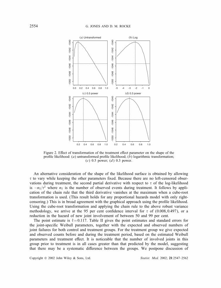
for a range of values of �. For � untransformed this pro�le log-likelihood graph is far fromsymmetric, as can be seen in Figure 2(a). The natural transformation here would be to log �since this removes the boundary �=0; it is also the usual parameterization in the Cox model.However the pro�le likelihood for log � is still far from symmetrical; in fact it errs in theopposite direction to that of the untransformed � (Figure 2(b)). The problem here seems tobe that, as noted earlier, very few uninvolved joints became involved during treatment, andit is only these which prevent � from being zero. To apply the robust variance estimatorin constructing a con�dence interval, we seek a transformation which will approximatelysymmetrize the pro�le log-likelihood. In Figure 2(c) we show the pro�le log-likelihood forthe 0.5 power, and in Figure 2(d) we show the plot for 0.3, which appears to be a suitablechoice.



(a) Untransformed

0.0 0.2 0.4 0.6 0.8 1.0

-105

0-1

048

-104

6-1

044

-104

2-1

040

(b) Log

-5 -4 -3 -2 -1 0

-105

0-1

048

-104

6-1

044

-104

2-1

040

(c) 0.5 power

0.2 0.4 0.6 0.8 1.0

-105

0-1

048

-104

6-1

044

-104

2-1

040

(d) 0.3 power

0.2 0.4 0.6 0.8 1.0

-105

0-1

048

-104

6-1

044

-104

2-1

040

Figure 2. E�ect of transformation of the treatment e�ect parameter on the shape of thepro�le likelihood: (a) untransformed pro�le likelihood; (b) logarithmic transformation;

(c) 0.5 power; (d) 0.3 power.

An alternative consideration of the shape of the likelihood surface is obtained by allowing� to vary while keeping the other parameters �xed. Because there are no left-censored obser-vations during treatment, the second partial derivative with respect to � of the log-likelihoodis −nT=�2 where nT is the number of observed events during treatment. It follows by appli-cation of the chain rule that the third derivative vanishes at the maximum when a cube-roottransformation is used. (This result holds for any proportional hazards model with only right-censoring.) This is in broad agreement with the graphical approach using the pro�le likelihood.Using the cube-root transformation and applying the chain rule to the above robust variancemethodology, we arrive at the 95 per cent con�dence interval for � of (0:008; 0:497), or areduction in the hazard of new joint involvement of between 50 and 99 per cent.The point estimate is �=0:117. Table II gives the point estimates and standard errors for

the joint-speci�c Weibull parameters, together with the expected and observed numbers ofjoint failures for both control and treatment groups. For the treatment group we give expectedand observed counts before and during the treatment period, based on the estimated Weibullparameters and treatment e�ect. It is noticeable that the number of involved joints in thisgroup prior to treatment is in all cases greater than that predicted by the model, suggestingthat there may be a systematic di�erence between the groups. We postpone discussion of



Table II. Estimated Weibull parameters (standard errors in parenthesis) from the marginal model, with ex-pected (observed) joint failures for the control group and the treatment group before and during treatment.

Joint � � Control Before During

Neck 0.181 (0.033) 0.85 (0.13) 36.5 (37) 16.5 (21) 0.32 (0)Spine 0.149 (0.022) 0.99 (0.15) 36.0 (35) 15.9 (21) 0.37 (0)Jaw 0.043 (0.003) 2.05 (0.36) 25.4 (26) 5.6 (6) 0.26 (0)Shoulders 0.136 (0.018) 1.09 (0.15) 71.4 (74) 31.0 (36) 0.82 (0)Elbows 0.044 (0.006) 1.11 (0.13) 50.5 (52) 15.8 (16) 0.49 (1)Hips 0.060 (0.006) 1.19 (0.21) 58.3 (59) 19.6 (29) 0.62 (0)Knees 0.041 (0.003) 1.81 (0.23) 49.0 (50) 11.2 (14) 0.49 (1)

this until Section 5. We also note that if the expected number of joint involvements duringtreatment is calculated conditional on the observed number of failures prior to treatment, thesebecome 0.19, 0.22, 0.36, 0.29, 0.35.To investigate the validity of the robust variance approach, which is based on an asymptotic

approximation, we simulated new data sets using the estimated parameter values of our model,keeping the same censoring times (that is, the ages of patients at interview, or start and endof treatment). To simulate correlated Weibulls with the given marginals we started with11-dimensional standard normals, transformed these to equicorrelated normals, squared andadded pairs to give correlated 11-dimensional exponentials, and then used the joint-speci�cparameters to convert the components to Weibulls. The degree of correlation is controlledby the o�-diagonal element r in the matrix used to transform the standard normals, thecorrelation in the transformed normals being (2r+9r2)=(1+10r2). Values of 0.1, 0.2, 0.3, 0.4give correlations of 0.26, 0.54, 0.74, 0.86, respectively, thus ranging from fairly weak to quitestrong correlation between the within-patient joint failure times. Based on 5000 simulationseach, we found that the rates of inclusion of the true value of � of nominal 95 per centcon�dence intervals, using robust variance with the cube-root transform, were 95.7, 93.5,91.4 and 90.4 per cent, respectively. Thus there appears to be a deterioration in performanceas the strength of the correlation increases. To match the actual data to the simulation resultswe estimated within-patient correlations using the observed failure times and matched theseinformally with the correlations in the simulated data, which suggested that our data areclosest to r=0:3. Thus our 95 per cent interval is perhaps closer to 90 per cent in coverage.The averages of the robust standard errors of the cube-root transformed treatment e�ect foreach set of simulations were, respectively, 0.0847, 0.0845, 0.0849, 0.0862; the correspondingstandard deviations of the point estimates were 0.0852, 0.0883, 0.0923, 0.0968. This seems tosuggest that some form of parametric bootstrap might be a better procedure, but this wouldrequire a parametric model of the dependence. Moreover, neither the parametric nor the non-parametric bootstrap will work with our data because many of the bootstrap samples haveno observed failures on treatment, resulting in an in�nite estimated treatment e�ect (�=0).Thus the use of the asymptotic robust variance, while not ideal, would seem to be the onlytractable method, and is greatly improved by the cube-root transform.

4. FRAILTY MODEL

Here we take the hazard rate for patient i to be of the form hi(t)=Zih0(t) where h0(t) isa baseline hazard which might depend on covariates such as, in our case, treatment with



Accutane. The frailties {Zi} are usually assumed to come from a parametric family of dis-tributions, for example the gamma distribution with mean 1. This gamma family is oftenconvenient for estimation via the EM algorithm, the frailties being regarded as unobserveddata. If the Cox partial likelihood is used, the frailties Zi enter linearly into that part of thelog-likelihood which depends on the regression and gamma parameters, and the conditionalexpectation of each Zi is also easy to calculate.In the presence of double-censoring, however, this convenience is lost. There is no partial

likelihood, and the left-censoring introduces terms of the form (1 − e−ZiHij(�; t)) into the fulllikelihood so that the EM algorithm becomes intractable. When the terms for the ith person aremultiplied out we get the sum of terms of the form Znii e

−ZiKij(�; t), so the assumption of a gammadistribution still allows the frailties to be integrated out of the likelihood reasonably simply.However the resulting function is extremely complex in its dependence on the regressionparameters � and the baseline survivor functions, so for highly multivariate problems such asours a direct maximization of the likelihood is again intractable. Our approach instead is touse the conditional independences in the model as much as possible, iteratively estimating thefrailties Zi and the survivor function parameters �j; �j to maximize the complete likelihoodfor each value of the parameters of interest, and to base inferences on these parameters onthe resulting pro�le likelihood.Frailties are easily incorporated into our model, the survival function for an individual with

frailty Zi becoming

Sj(t|Zi)={e−Zi(�jt)

�j in the control groupe−�Zi(�jt)

�j in the treatment group(1)

The treatment e�ect is here assumed to have a multiplicative e�ect on the conditional hazardshj(t|Zi).Our approach to the treatment of the frailties is similar to that used by McGilchrist and

Aisbett [17] to �t a frailty model to bivariate catheter infection data. They �rst consider thefrailties to be �xed e�ects, which they estimate together with a regression parameter � bymaximizing the log-likelihood L(z; �) subject to the constraint

∑log(Zi)=0. They use the

Cox model so their log-likelihood comes from the Cox partial likelihood. They then consideran alternative random e�ects model in which the log frailties are Gaussian with zero meanand unknown variance. They construct a ‘penalized likelihood’ by augmenting the previouslog-likelihood of the observations with z conditionally �xed by the likelihood of z as givenby the log-normal frailty distribution. This is again maximized subject to the same constrainton the vector z of frailties. This second alternative can be thought of as a hierarchical modelin which the log Zi for each patient is �rst chosen from N(0; �2) and then the observationsarise from the conditional distributions given Zi. This approach is generally preferred becausedirect maximization over a large number of nuisance parameters as in the �rst method islikely to produce inconsistent estimates.Taking the �rst approach, in which the Zi are regarded as �xed e�ects, our model gives

the log-likelihood as

L(�; z; �)=∑i

∑j‘ij(�; Zi; �j; �j)

where z is the vector of frailties and � the vector of Weibull parameters. Inference for � canbe based on the pro�le likelihood [18]; for each �xed � we maximize the above expression



over z; �. There is an identi�ability problem since we can replace z by kz and �j by (�j=k)1=�jfor any positive scalar k without changing the likelihood, so we impose

∑log(Zi)=0. To

achieve the optimization we use the following iterative scheme:

1. Initialize Zi≡ 1.2. For each joint type j calculate the conditional maximum likelihood estimates for theWeibull parameters �j; �j given z by maximizing

∑i ‘ij(�; Zi; �j; �j).

3. For each subject i calculate the conditional maximum likelihood estimate for Zi given� by maximizing

∑j ‘ij(�; Zi; �j; �j).

4. Adjust z to satisfy the constraint, multiplying each Zi by e−∑

i log(Zi)=n.5. Repeat steps 2–4 until convergence.

We note that step 4 is not necessary for convergence but is necessary for identi�abil-ity of the model. By using alternating conditional maximum likelihood estimators we areable to replace a complex multiparameter optimization by a number of simpler univari-ate and bivariate ones. Repetition over a range of values of � can be expedited by us-ing the �nal z and � from the previous � as starting values for the next. The estimateis �=0:031, and using the usual asymptotic �2 approximation to the logged likelihood ra-tio gives the 95 per cent con�dence interval (0:005; 0:098). Each pro�le likelihood calcu-lation also yields estimates of the frailties z of the individuals in the study. The obviousapproach here would be to use the estimates of z at the maximizing values of � and �.These might be of some clinical interest, but the estimates are likely to be unreliable be-cause of the large number of parameters involved. Figure 3 shows kernel-smoothed den-sity estimates for these estimated log frailties, separately for each group. There is againsome suggestion of a di�erence between the control and treatment groups, to be discussed inSection 5.Turning now to the second approach, we consider a hierarchical model in which the Zi are

random drawings from some ‘frailty distribution’. Figure 3 suggests that the log frailties areapproximately normal, so we follow McGilchrist and Aisbett [17] in using penalized likelihoodwith a log-normal distribution, but di�er slightly in that we consider the Zi to be independentof each other, whereas they specify a multivariate distribution for z which incorporates theconstraint

∑log(Zi)=0. This constraint is no longer necessary for identi�ability because of

the penalty term, but it will be satis�ed by the maximum likelihood estimates. We thereforecontinue to impose the constraint, not as part of the model but as part of the estimationprocedure.Our main focus of interest is again �, but it may also be relevant to examine the ‘frailty pa-

rameter’ �. For �xed (�; �) we maximize the likelihood over the Weibull andfrailty parameters following steps 1–5 to give the ‘penalized pro�le likelihood’

LP(�; �)= max�; �; z

{∑j‘ij(�; Zi; �j; �j)− 61 log � − (log Zi)2

2�2

}

Evaluating this over a grid of values allows examination of the likelihood surface, as inFigure 4, which shows max�; �LP(�; �)−LP(�; �); the contour corresponding to level 3 is anapproximate asymptotic 95 per cent con�dence region. This suggests that log � is signi�cantlyless than zero, pointing again to a signi�cant reduction in hazard with Accutane use. Thepoint estimate for (�; �) is (0.059, 0.94).



logFrailty

dens

ity

-2 0

0.0

0.1

0.2

0.3

0.4

Control Group Treatment Group

2 4

Figure 3. Kernel density estimates of the frailty distribution for the control and treatment groups.

logTau

Sig

ma

-5 -4 -3 -2 -1 0

0.6

0.8

1.0

1.2

1.4

1.6

0.050.2 1 2

3 35 5 10

20

30

Figure 4. Penalized pro�le likelihood for the treatment and frailty parameters in the frailty model.



5. TESTING FOR GROUP DIFFERENCES

The above analysis assumes that the treatment and control groups are comparable, in that theyhave the same baseline survival functions in the marginal model or the same frailty distributionin the frailty model. Since the allocation was not done on the basis of a randomized trial, theremay be systematic di�erences between the groups which would a�ect and perhaps invalidateour inference about the treatment e�ect. We have noted two possible sources of bias: di�erentrecruitment criteria and di�erent diagnosis of joint involvement. The second of these couldperhaps be accommodated by arguing that the more sensitive radiographical diagnosis appliedto the treatment group would tend, if anything, to diminish the apparent e�ectiveness of thetreatment, but little can be said about the �rst. Furthermore there may be omitted covariatescausing a di�erence between groups.We saw in the �tted marginal model, from Table II, that the treatment group had a higher

than expected number of joint involvements prior to the commencement of the treatmentperiod, particularly in the neck and spine regions. Since these were determined by radiologicalscans it is possible that in many cases immobilization of the joint had not yet occurred, sothat some of these would not be classed as involved using the control group criterion.It was noted in Section 4 that the frailty analysis suggests, from Figure 3, that there is a

systematic di�erence between the groups, with the treatment group having higher frailties thanthe control group: this e�ect, though reduced, still exists when a parametric family is usedto model the frailties. This again is consistent with the more sensitive diagnostic techniquesused in the clinical examinations. These di�erences are incorporated into the estimation ofthe treatment e�ect; if we eliminated the di�erence by forcing the log frailties to sum to zeroseparately for each group, this would then reduce the estimated frailties for the treatmentgroup and hence reduce the apparent e�ectiveness of the treatment. It might be better in suchsituations to assume di�erent distributions for the frailties in the control and treatment groups.It should be noted that since the treatment is time-dependent, with some information avail-

able on the treatment patients before their treatment began, it would be possible to estimate �using only this group. This does not work well in practice because there are only 21 subjectsand nearly all the observations are either right- or left-censored. We can however use this pre-treatment information to examine possible di�erences between the groups. Using the marginalmodel approach we can subsume any recruitment, diagnostic and covariate di�erences into asingle group di�erence parameter , assumed to have a multiplicative e�ect on the marginalhazard rates for the treatment group. Proceeding as before, we use a working independencemodel to estimate . The contributions to the working log-likelihood for the ith treatmentgroup patient are now

‘ij(�j; �j)=

{ log Sj(si) if �ij=0

log(1− [S(si)]) if �ij=2

with all observations being either left- or right-censored according to their status at the time ofcommencement of the treatment period. This gives =1:84 so the pre-treatment informationsuggests that if anything the treatment group are more prone to joint involvement than thecontrols at baseline, perhaps because of the more sensitive radiological diagnosis. This wouldtend to strengthen our conclusions about the e�ectiveness of the Accutane treatment. Howeverthe robust variance estimate gives the standard error of as 0.81, and the pro�le likelihood



for the untransformed parameter is reasonably symmetric, so the estimated group di�erence isnot signi�cantly di�erent from =1. It seems reasonable then, given the limited informationavailable, to proceed with the assumption of no group di�erences.

6. DISCUSSION

We have considered two di�erent methods of trying to accommodate the within-patient de-pendence in multivariate survival analysis. Both approaches are su�ciently common in theliterature to be considered standard (see for example Klein and Moeschberger [19]), but untilnow both the application and much of the theory has used partial likelihood in the Cox model.When there is double censoring, considerable adaptation is required. In particular there seemsnow to be no alternative to the estimation of the baseline survival functions, which bringsboth computational and inferential di�culties. These di�culties are further increased when wemove from bivariate data, which has been the norm in the literature, to highly multivariatedata (p=11). Here we have taken a parametric approach to the modelling of the survivalfunctions, but adapting it to a semi-parametric model in which the survivor functions areestimated non-parametrically would be very challenging. We have also had to assume thatthe treatment e�ect, and the frailties in the frailty model, are the same for each joint. Ideallyone would want to check these assumptions, but given the sparsity of our data we have beenunable to do so. The elbow and knee joints had one failure each during treatment, leading tocon�dence intervals of (0.015, 1.03) and (0.019, 1.09), respectively. It is clear from these thatthere is not enough data on individual joint failures to estimate and compare joint-speci�ctreatment e�ects. There seems no alternative to the assumption that the e�ect of Accutaneis homogeneous. We have noted that both joint failures a�ected the same patient. While itmay be extreme to suppose that only this patient received no protection from Accutane, itis probably also extreme to suppose that Accutane protects every patient equally. Again wefound no tractable alternative to the strong assumption made.The most important conclusion is shared by both the marginal and frailty approaches;

Accutane treatment leads to a signi�cant reduction in the rate of involvement of previouslyuna�ected joints. It is important to note however that the two approaches lead to di�erentinterpretations of the treatment e�ect, and to di�erent marginal distributions for the jointinvolvements. The marginal model assumes that Accutane has the same multiplicative e�ect oneach of the marginal hazard rates, and that the marginal distributions are Weibull. The frailtymodel assumes that Accutane has the same multiplicative e�ect on each of the conditionalhazard rates of an individual given their frailty, and that the conditional distributions areWeibull. If we were to integrate out the frailty we would �nd that the marginal distributionswere not Weibull, and that the e�ect of Accutane was not proportional on the marginalhazard. Since the Weibull model was originally chosen by examining the marginal distributions(Section 2), we might want to question the parametric forms used in the frailty model. Thelog-normal frailty distribution was chosen by examining the unrestricted frailty estimates,but other choices could have been made. The gamma distribution is a common choice, butits convenience is lost with double censoring. Hougaard [20] recommends a positive stabledistribution since this preserves proportional hazards in the margins.Both approaches as implemented here involve a large number of nuisance parameters, which

given the small amount of data must raise concerns about the asymptotic results used. This



is particularly true for the frailty model. With the frailties as �xed parameters there are in all76 parameters and 671 observations. It is clearly preferable to regard the frailties as randome�ects, and the penalized likelihood approach does this, although ideally one would want tointegrate the frailties out of the likelihood. This seems to be intractable with doubly-censoreddata. We have made some savings on the number of parameters by assuming that right–left pairs of joints have the same baseline hazards; that is, the same Weibull parameters. InTable II the � parameters seem di�erent for the hip and especially the knee joints, althoughthese parameter values are not precise as evidenced by the large standard errors. Ideally wewould like to test simultaneously the equality of all eight pairs of parameters, but the usuallikelihood ratio test does not apply because it ignores within-patient correlation. A referee hassuggested that di�erences between pairs might explain the lack of �t for hip in the treatedgroup (Table II). However, the 29 pre-treatment failures comprise 14 left and 15 right hips.The lack of �t in this column is evidence that the treatment group appear to be more frail,as discussed in Section 5. That this frailty seems particularly pronounced for the hip joints isan interesting observation, but not one that we can explain.An advantage of the marginal approach is that it applies without our having to specify the

type of dependence between joints. The frailty model assumes that these are conditionallyindependent given the frailty, which may not be a reasonable assumption; although the mech-anism is not known, some clinicians believe that the disease progresses in a characteristicpattern [2; 21]. The frailty model approach is, however, of added interest since it provides(through the frailty parameter �) information about the range of di�erences in the severity ofthe disease which might be useful to clinicians; estimates of individual frailties could also behelpful in predicting prognosis for individual patients.

ACKNOWLEDGEMENTS

We thank Jeannie Peeper, Dr Michael Zaslo� and Dr Frederick S. Kaplan for providing the data, andtwo anonymous referees for helpful comments and suggestions.

REFERENCES

1. Kaplan FS (ed.). Clinical Orthopaedics and Related Research. Lippincott-Raven: Philadelphia, 1998.2. Cohen RB, Hahn GV, Tabas JA, Peeper J, Levitz CL, Sando A, Sando N, Zaslo� M, Kaplan FS. The naturalhistory of heterotopic ossi�cation in patients who have �brodysplasia ossi�cans progressiva. Journal of Boneand Joint Surgery 1993; 75-A:215–219.

3. Wei LJ, Lin DY, Weissfeld L. Regression analysis of multivariate incomplete failure time data by modellingmarginal distributions. Journal of the American Statistical Association 1989; 84:1065–1073.

4. Huber PJ. The behaviour of maximum likelihood estimates under non-standard conditions. Proceedings of theFifth Berkeley Symposium on Mathematical Statistics and Probability 1967; 1:221–233.

5. Clayton DG. A model for association in bivariate life tables and its application in epidemiological studies ofchronic disease incidence. Biometrika 1978; 65:141–151.

6. Vaupel JW, Manton KG, Stallard E. The impact of heterogeneity in individual frailty on the dynamics ofmortality. Demography 1979; 16:439–454.

7. Oakes D. A model for association in bivariate survival data. Journal of the Royal Statistical Society, SeriesB 1982; 44:414–422.

8. Clayton DG, Cuzick J. Multivariate generalisations of the proportional hazards model. Journal of the RoyalStatistical Society, Series A 1985; 148:82–117.

9. Huster JH, Brookmeyer R, Self SG. Modelling paired survival data with covariates. Biometrics 1989;45:145–156.

10. Finkelstein DM. A proportional hazards model for interval-censored failure time data. Biometrics 1986; 42: 845–854.



11. Alioum A, Commenges D. A proportional hazards model for arbitrarily censored and truncated data. Biometrics1996; 52:512–524.

12. Satten GA. Rank-based inference in the proportional hazards model for interval censored data. Biometrika 1996;83(2):355–370.

13. Goggins WB, Finkelstein DM, Zaslavsky AM. Applying the Cox proportional hazards model when the changetime of a binary time-varying covariate is interval censored. Biometrics 1999; 55:445–451.

14. Zaslo� MA, Rocke DM, Cro�ord LJ, Gregory VH, Kaplan FS. Treatment of patients who have �brodysplasiaossi�cans progressiva with isotretinoin. Clinical Orthopaedics and Related Research 1998; 346:121–129.

15. Rocke DM, Zaslo� M, Peeper J, Cohen RB, Kaplan FS. Age- and joint-speci�c risk of heterotopic ossi�cationinpatients who have �brodysplasia ossi�cans progressiva. Clinical Orthopaedics and Related Research 1994;301:243–248.

16. Turnbull BW. Nonparametric estimation of a survivorship function with doubly censored data. Journal of theAmerican Statistical Association 1974; 69:169–173.

17. McGilchrist CA, Aisbett CW. Regression with frailty in survival analysis. Biometrics 1991; 47:461–466.18. Kalb�eisch JD, Sprott DA. Application of likelihood methods to models involving large numbers of parameters.

Journal of the Royal Statistical Society, Series B 1970; 32:175–209.19. Klein JP, Moeschberger ML. Survival Analysis: Techniques for Censored and Truncated Data. Springer-Verlag:

New York, 1997; 405–418.20. Hougaard P. Survival models for heterogeneous populations derived from stable distributions. Biometrika 1986;

73:387–396.21. Kaplan FS, Tabas JA, Zaslo� MA. Fibrodysplasia ossi�cans progressiva: a clue from the �y? Calci�ed Tissue

International 1990; 47:117–125.


Multivariate survival analysis with doubly-censored data: application to the assessment of Accutane...

Documents

Transcript of Multivariate survival analysis with doubly-censored data: application to the assessment of Accutane...