Multivariate Resolution in Chemistry Lecture 3 Roma Tauler IIQAB-CSIC, Spain e-mail:...

Multivariate Resolution in Chemistry

Lecture 3

Roma TaulerRoma TaulerIIQAB-CSIC, Spain

e-mail: [email protected]

Lecture 3

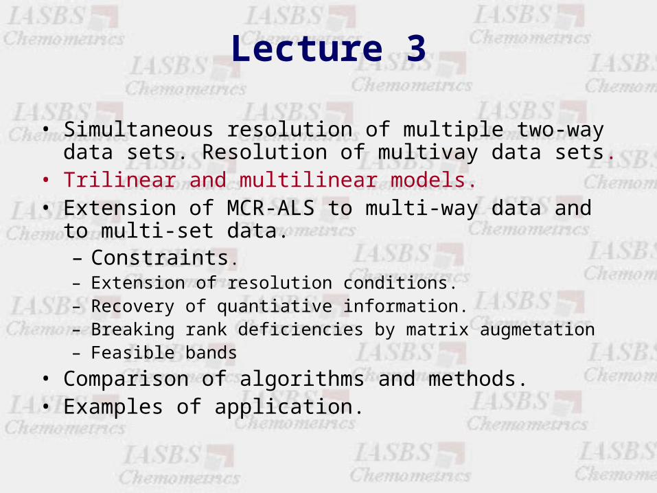
• Simultaneous resolution of multiple two-way data sets. Resolution of multivay data sets.

• Trilinear and multilinear models. • Extension of MCR-ALS to multi-way data and to multi-set

data. – Constraints. – Extension of resolution conditions. – Recovery of quantiative information. – Breaking rank deficiencies by matrix augmetation– Feasible bands

• Comparison of algorithms and methods. • Examples of application. (1.5 hours)

Luminiscenceexcitacion /emission spectra/sample

Process/Reaction spectroscopic monitoringtime/pH/temperaturewavelengthsample/system/run

Analytical Hyphenated Methods:LC/DAD; LC/FTIR; GC/MS; LC/MStime/wavelength/sampletime/m/z ratios/sample

Environmental monitoringsamples/concentrations/time or conditions

Spectroscopic imagingmultiple spectroscopic images from differentsamples

……

Examples of Three-way data in Chemistry

Three-way data in Chemistry

Example: Multiple excitacion emission spectra (standards and unknown samples)

Wavelengths

wav

elen

gths

sample

number

emission

exc

itatio

n

samples

exci

tati

on

emission

samples.

* * * *

** **

* * * *

*

Three-way data in ChemistryExample: Multiple HPLC-DAD-MS runs of a

system (standards and unknown samples)

Wavelengths

Elu

tion

tim

e

Run

number

Spectrum

Ch

rom

ato

gra

m

runs

chro

mat

ogra

m

spectrum

runs.

* * * *

** **

* * * *

*λ

m/ztR

λm/z

tR

Three-way data in ChemistryExample: A chemical reaction or proces monitored

spectrsocopically

Process

number

time

spectra

reac

tion

pr

ofile

s proce

ss.

Rea

ctio

n p

rofi

les

spectra

process

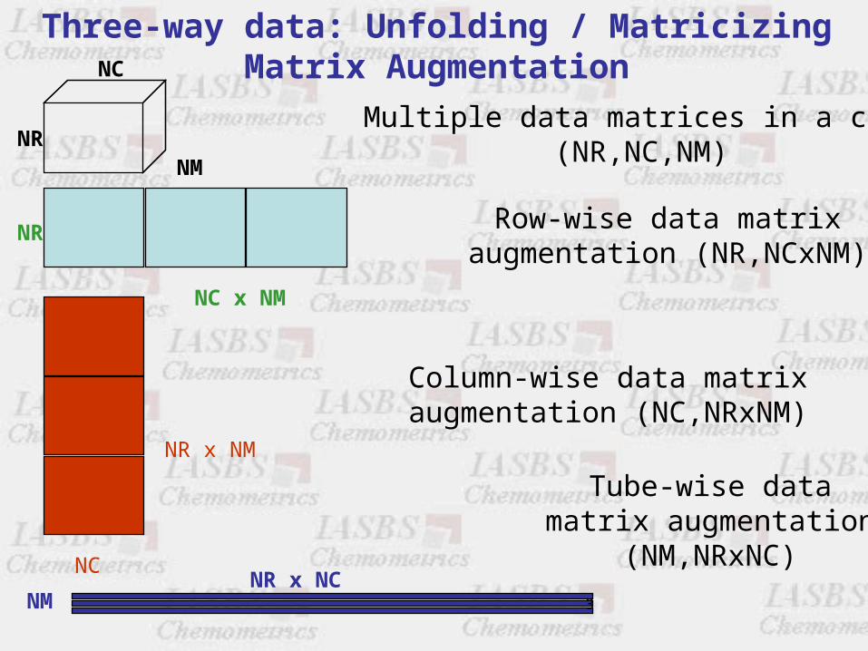
Three-way data: Unfolding / MatricizingMatrix AugmentationNC

NR NM

NR

NC x NM

NR x NM

NCNR x NC

3

Multiple data matrices in a cube(NR,NC,NM)

Row-wise data matrixaugmentation (NR,NCxNM)

Column-wise data matrix augmentation (NC,NRxNM)

Tube-wise datamatrix augmentation

(NM,NRxNC)

NM

Multiple data sets (e.g. environmental data)

Extension of Bilinear Models (PCA or MCR) Matrix Augmentation

The same experiment monitored with different techniques

=

D1

D2

D3

D

C1

=

D1

D2

D3

D

Several experiments monitored with the same technique

=

D1 D2 D3

D4 D5 D6

=

D1 D2 DC1

D4 D5 D6

CD Several experiments monitored with several

techniques

Row-wise

Column-wise Row and column-wiseD

=D1 D2 D3

D

=D1 D2 D3

D

=D1 D2 D3D1 D2 D3

S1T

C

CS2

T S3T

S1T S2

T S3T

ST

C2

ST

ST

C2

C3

C

0 20 40 600

2

4

6x 10

4

0 50 1000

2

4

6x 10

4

0 20 40 600

1

2

3x 10

4

0 50 1000

1

2

3x 10

4

0 50 1000

2

4x 10

4

0 20 40 600

2

4x 10

4

0 20 40 600

1

2

0 50 1000

2

4x 10

4

0 20 40 600

1

2

0 50 1000

5000

10000

15000

0 50 1000

5000

10000

15000

0 20 40 600

0.5

1

1.5

D1

D2

D3

DT1

DT2

DT3

B

A

A BC

Ex. Hyphenated Chromatography

Column-wisedata matrixaugmentation

=

D1

D2

D3

D

C1

=

D1

D2

D3

D

ST

C2

C3

C

D1 . Mixture matrix formed by A, B (analytes) and C (interferent).D2 . Standard of A. D3 . Standard of B.

0 500

0.02

0.04

0.06

0.08

0.1

0 50-10

-5

0

5

10

15

20

0 500

0.02

0.04

0.06

0.08

0.1

0 50-10

-5

0

5

10

15

20

0.05

0.15

0 500

0.1

0.2

0 50-10

-5

0

5

10

15

0 20 400

0.2

0.4

0.6

0.8

1

0 20 400

0.2

0.4

0.6

0.8

1

Ex. CD-UV absorption monitoring of a protein folding process

D1,UV D1,CD C1

SUVT SCD

T

C2D2,UV D2,CD

UV CD

1

2

UV CD

Process

ST

Dk Ck

(I x J) (I,n)

ST

(n,J)

Dk

Dk Ck

(I x J) (I,n)

ST

(n,J)

PCA: orthogonality; max. variance

MCR: non-negativity, nat. constraints

Stretched/unfolded representation ?

Dk = Ck ST = C tk ST

Ck

Daug

Caug

Extension of Bilinear models for simultaneous analysis of multiple two way data sets

Bilinear models to describe augmented matrices

Matrix augmentation

strategy

Lecture 3




• Comparison of algorithms and methods. • Examples of application.

D= C

ST

T

PARAFAC (trilinear model)

The same number of components In the three modes: Ni = Nj = Nk = N

No interactions between components

Different slices Dk are decomposed In bilinear profiles having the same shape!

Tk k

N

ijk in jn kn ijkn=1

D = CT S + E

d = c t s + e

PARAFAC trilinear model

N

N

D=

C

ST

T

NR NC

N

NM

N

1nijkknjninijk etscd

D = + + E+ ... +

comp 1 comp 2 comp 3 ...... error/noise

d c s t eijk in jn kn ijkn

N

1

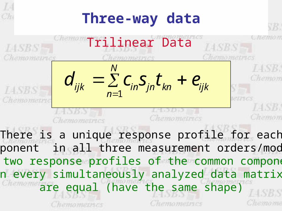
Three-way data

Trilinear Data

There is a unique response profile for eachcomponent in all three measurement orders/modes.

The two response profiles of the common componentsin every simultaneously analyzed data matrix

are equal (have the same shape)

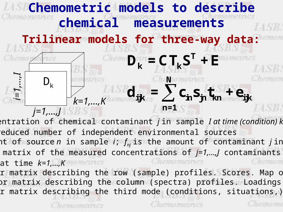
dijk is the concentration of chemical contaminant j in sample I at time (condition) kn=1,...,N are a reduced number of independent environmental sourcescin is the amount of source n in sample i; fnj is the amount of contaminant j in source nDk is the data matrix of the measured concentrations of j=1,...,J contaminants ini=1,...,I samples at time k=1,…,KC is the factor matrix describing the row (sample) profiles. Scores. Map of the samplesST is the factor matrix describing the column (spectra) profiles. Loadings. Map of variablesT is the factor matrix describing the third mode (conditions, situations,) T={Tk}

Tk k

N

ijk in jn kn ijkn=1

D = CT S + E

d = c s t + e

Chemometric models to describechemical measurements

Trilinear models for three-way data:

k=1,...,Ki=1,

...,I

j=1,...,J

Dk

Three Way data models

C ST

Np Nq Nr

I J

KC-mode D

S-mode

T-mode

(I , J , K)

variables

sam

ples

cond

itions

In generalNp, Nq and Nr may be different,

DC-mode

S-mode

T-mode

C STT

Np Nq Nr

Three-way data models

Np Nq Nr

ijk pqr ip jq kr ijk

p 1 q 1 r 1

d = g c s t e

variables

sam

ples

conditions

D

C

STG

T

(Np,Nq,Nr)=

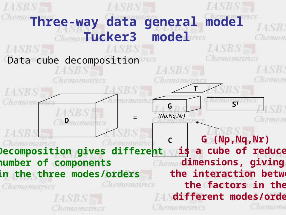
Three-way data general modelTucker3 model

Data cube decomposition

Decomposition gives differentnumber of componentsin the three modes/orders

G (Np,Nq,Nr)is a cube of reduceddimensions, giving

the interaction betweenthe factors in the

different modes/orders

D

C

STG

T

=•Different number of componentsin the different modes Np Nq Nr

•Interaction between components in different modes is possible

In PARAFAC Np = Nq = Nr = N andcore array G is a superdiagonal identity cube

Tucker3 models

Np Nq Nr

ijk pqr ip jq kr ijk

p 1 q 1 r 1

d = g c s t e

D=

C

STG

T

(N x N x N)

Three-way trilinear restricted modelPARAFAC model

Data cube decomposition

It is the Identitycube G = I

It may be omitted!!!

N


Decomposition gives the samenumber of componentsin all three modes/orders!!!

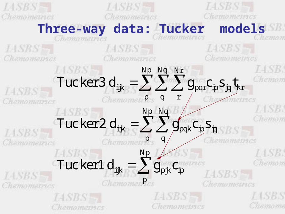
Np Nq Nr

ijk pqr ip jq krp q r

Np Nq

ijk pqk ip jqp q

Np

ijk pjk ipp

Tuc ker 3 d g c s t

Tuc ker 2 d g c s

Tuc ker1 d g c

Three-way data: Tucker models

Lecture 3





D1

D2

D3

ST

C1

C2

C3

T

=

D C

Multivariate Curve resolution Alternating Least Squares MCR-ALS

quantitative information

row-, concentration profiles

column-, spectraprofiles

column-wiseaugmenteddata matrix

NR1

NR2

NR3

NC

NM = 3

Different row sizes

Bilinear Model MCR-ALS of column-wise augmented data matrices

1 1 1

2 2 2

n n n

D C E

D C ET= S.... .... ....

D C E

Unconstrained Alternating Least Squares solution

1 1 1

2 2 2T T

n n n

+C D D

C D D +1) S = 2) C = S

.... .... ....

C D D

Optional constraints are applied at each ALS iteration!!!

+ matrix pseudoinverse calculation

MCR-ALS constraints for three-way data (simultaneous analysis of a set of correlated

bilinear data matrices)

• Same constraints as those applied to individual data matrices (non-negativity, unimodality, closure, local rank, ...).

• Correspondence between common species in the different data matrices

• Extension of resolution theorems to augmented data matrices (local rank conditions)

• Non-trilinear Data– Column profiles (spectra) of the common components are

forced to be equal in all the simultaneously analyzed data matrices

• Trilinear data (trilinearity constraint)– Column and row profiles of the common components are

forced to be equal in all the simultaneously analyzed data matrices (trilinearity)

Constraints applied to individual data matrices

Like in MCR-ALS for two-way data, but separatelyfor each data matrix and species

non-negative profiles (concentration, spectra, elution,...)unimodal profilesclosure, mass-balance,...shape (gaussian, assimetric,...) selectivity, local rank ..............

MCR-ALS constraints for three-way data


Correspondence between commonspecies in the different data matrices

SpeciesB + C

SpeciesA + B

SpeciesA+B+C+D

=

SpeciesA B C D

000

D1

D2

D3

D1

D2

D3

ST

000

000000

[C1;C2;C3][D1;D2;D3]

xxx

xxxxxx

xxx

xxx

xxx

xxx

xxx

Zero values give selectivity and local rank resolution conditions!!!!Appropriate design of experiments will help for total resolution andremove of rotational ambiguities!!

Xaug

D

YT

contaminants

compartments

site

s

FS

W

F

S

W

contaminants

site

ssi

tes

site

s

1

2

3

4

5

6

PCAMCR-ALS

Bilinear modelling of three-way data(Matrix Augmentation, matricizing, stretching, unfolding )

SVD1 2 3 x

i

SVD4 5 6 xii

z

i

z

ii

Scores refolding

strategy!!!(applied to augmented

Scores)

X Y

Z

site

s

contaminants

compartments (F,S,W)

x

i

xii z

iz

ii

Loadings recalculationin two modes

from augmentedscores

Chemometrics and Intelligent Laboratory Systems, 2007, 88, 69-83

D

contaminants

compartments

site

s

F

S

W

F

S

W

contaminants

site

ssi

tes

site

s

Xaug

YT

1

2

3

MCR-ALS

TRILINEARITY CONSTRAINT(ALS iteration step)

Selection of species profile

1

2

3

Folding

every augmentedscored wnated tofollow the trilinearmodel is refolded

MA-MCR-ALSTrilinearity constraint

SVD

Substitution ofspecies profile

Rebuilding augmented scores

1’

2’

3’



X YT

contaminants

Z

site

s


This constraintis applied at each stepof the ALS optimization

and independently for each component

individually

ST

C

=

D

D1

D2

D3

Trilinearity can be implemented independently for each component (chemical species) in MCR-ALS!

1st scoreloadings

PCA,SVD

Foldingspeciesprofile

1st scoregives thecommonshape

Loadings give therelative amounts!

Trilinearity Constraint

Unfolding species profile

UniqueSolutions!

Substitution of species profile

C

Selection of species profile

Effect of application of the trilinearity constraint

Profiles withdifferentshape

Profiles withequal shape

Trilinearityconstraint

0 50 100 150 200 2500

0.1

0.2

0.3

0.4

0.5

0.6

0.7

0.8

0.9

1

0 50 100 150 200 2500

0.1

0.2

0.3

0.4

0.5

0.6

0.7

0.8

Run 2

Run1Run 3

Run 4

Run 2

Run1Run 3

Run 4

one profile in C augmented data matrix

D

=

Xaug

Y

contaminants

compartments

site

s

F

S

W

F

S

W

metals

site

ssi

tes

site

s

1

2

3

4

5

6

MCR-ALS

Folding

1 2 3 4 5 6

component interaction constraint

(ALS iteration step)

interacting augmented scores are folded

together

1’

2’

3’

4’

5’

6’

=



MA-MCR-ALScomponent interaction

constraint

SVD =

This constraint is applied at each step of the ALS optimizationand independently and individually for each component i

XY

Z


This is analogous to a restricted Tucker3 model

Lesson 3



data. – Constraints. – Extension of resolution conditions. – Recovery of quantiative information. – Breaking rank deficiencies by matrix augmentation– Feasible bands


Extension of resolution theorems to augmented data matrices

• Resolution local rank conditions are more easily achieved for augmented ata matrices

• When resolution conditions are achieved for some component/species present in one of the single matrices, the resolution is also achieved for the same component/species in the rest of matrices (due to the correspondence between component/species!)


Lecture 3



data. – Constraints. – Extension of resolution conditions. – Recovery of quantitative information. – Breaking rank deficiencies by matrix augmetation– Feasible bands


In the simultaneous analysis of multiple data matricesintensity/scale ambiguities can be solved a) in relative terms (directly)b) in absolute terms using external knowledge

Solving intensity ambiguities in MCR-ALS

d c s c sij in nj

n

in nj

n

k1

k

k is arbitrary. How to find the right one?

Recovery of quantitative information

• Relative Quantitation

Unknown reference concn. Cr

C1/Cr = A1 / Ar

C2/Cr = A2 / Ar

• Absolute Quantitation

Known reference concn. Cr

C1 = (A1 / Ar) Cr

C2 = (A2 / Ar) Cr

0 10 20 30 40 50 600

1

2x 10

-5

0 10 20 30 40 50 600

1

2x 10

-50 10 20 30 40 50 600

1

2x 10

-5

C1

C2

Cr

interf.

interf.

referencesample

sample 2

sample 1

D1

D2

D3

=

NR

NR

NR

NS=4

NCC1

C2

C3

ST

E1

E2

E3

+

Quantitative MCR-ALS for three-way data

c11 c21 c31unfolding

profile 1c11

c21

c31

RelativeQuantitation

ratio of conc. profileareas: A12/A11, A13/A11....

ratio of conc. profile maximum intensitiesm21/m11, m31/m11,...

other .....

A11 A21 A31

m11 m21 m31

Quantitative informationin iterative three-way methods

(PARAFAC-ALS and Tucker-ALS)

Dk C Tk ST

=

(m x n) (m x c)

(c x c) (c x n)

tk

Quantitative information is available from matrix Tk

(third mode)!!

Lecture 3



data. – Constraints. – Extension of resolution conditions. – Recovery of quantiative information.– Breaking rank deficiencies by matrix augmentation – Feasible bands


Rank augmentation by matrix augmentationMatrix augmentation allows the study

of rank deficient systemsRank deficient systems are systems where the number of linearly independent components is lower than the number of the true contributions. In reaction based systems:

D = C ST

rank(D) = min(rank (C,ST)) rank(D)= min (R+1, Q)

R num. of reactions, Q num. of speciesRank augmentation can be obtained by matrix augmentation!

A B 2 species, 1 reaction, rank is 2A + B > C 3 species, 1 reaction, rank is only 2 (rank deficiency)A > B + C 3 species, 1 reaction, rank is only 2 (rank deficiency)A + B > C + D 4 species, 1 reaction, rank is only 2 (rank deficiency)A B C D 4 species, 2 reactions, rank is 3 (rank deficiency)............................................................................................

[ACU;A]

pH = 9.4

pH = 10.5

pH = 13.3

R1 R2

R3

Kinetic determinations Journal of Chemometrics, 1998, 12, 183-203

Acid-base spectrometric titrations: mixtures of nucleic bases : HA; U, HU; H, HH; T, HT Chemometrics and Laboratory Systems, 1997, 38, 183- 197

Rank deficiency is broken By means of matrix augmentation

Quantitative determinationswith errors < 3%

ACU

A

MCR-ALS

Lecture 3



data. – Constraints. – Extension of resolution conditions. – Recovery of quantiative information.– Breaking rank deficiencies by matrix augmentation– Feasible bands


Calculation of band boundaries of feasible solutions for three-way data

The same general optimization problem as for two-way data can be easily implemented and extended to column-wise augmented data matrices (three-way data).

Constraints are implemented in the same way as for two-way data (natural, local rank, selectivity...)

Additional constraints for trilinear data: Trilinearity constraint!!!

Extensión to ‘multiway’ data: 4 chromatographic

runs of 4 coeluting components Trilinear data

N


0 50 100 150 20000.20.40.60.8

11.21.41.61.8

Run 2Run1Run 3

Run 4 0 50 100 150 2000

1

2

3

0.5

0 20 4000.10.20.30.4

0 5 10 15 20 25 30 35 40 45 500

0.2

0.4

0.6

0 20 40 60 80 100 120 140 160 180 2000

1

2

3

4

Run 1 Run2 Run 3 Run 4

a) Matrix augmentation, non-negativity andspectra normalization constraints

0 10 20 30 40 50 60 70 80 90 1000

0.05

0.1

0.15

0.2

0.25

0.3

0.35

0 20 40 60 80 100 120 140 160 180 2000

0.5

1

1.5

2

2.5

3

c) Matrix augmentation, non-negativity, spectranormalization and trilinearity constraints

0 5 10 15 20 25 30 35 40 45 500

0.1

0.2

0.3

0.4

0.5

0.6

0 20 40 60 80 100 120 140 160 180 2000

1

2

3

4

b) Matrix augmentation, non-negativity, spectranormalization and selectivity constraints

• Resolution local rank/selectivity conditions are achieved in many situations for well designed experiments (unique solutions!)

• Rank deficiency problems can be more easily solved• Constraints (local rank/selectivity and natural constraints) can be

applied independently to each component and to each individual data matrix.

• Total resolution is achieved for three-way trilinear and for most of non-trilinear data systems

• The multilinear structure can be introduced in a flexible way as an additional constraint in the ALS algorithm (even for Tucker models with interaction among components)

J,of Chemometrics 1995, 9, 31-58; J.of Chemometrics and Intell. Lab. Systems, 1995, 30, 133

Advantages of MCR-ALS ofThree-way Data

Lecture 3



data. – Constraints. – Extension of resolution conditions. – Recovery of quantitative information.– Breaking rank deficiencies by matrix augmentation – Feasible bands


D= C

ST

T

Dk C Tk ST

=

(m x n) (m x c)

(c x c) (c x n)

tk

PARAFAC

D

C

STG

T

(r x c x t)=

Dk C

=

(m x n) (m x r)

ST

(c x n)

Nk

(r x c)

TUCKER

Nr

k kr rr 1

N t G

=

ST

D C

T

DkCk

=

(m x n) (m x c)

ST

(c x n)

MCR-ALS

Ck* = Ck Tk

Resolution of three-way data

• Trilinear data: factor analysis rotational ambiguities are totally solved– Examples of methods: GRAM, TLD, PARAFAC-

ALS, Tucker-ALS, MCR-ALS, ...• Non-trilinear data: Factor analysis rotational

ambiguities can still be present but they are solved in many situations under some constraints– Examples of methods: Tucker-ALS, MCR-ALS

Non-iterative (Eigenvector Decomposition)

GRAM (Generalized Rank Annihilation) TLD (Trilinear Data Decomposition)

Iterative (Alternating Least Squares, ALS)

PARAFAC-ALS Tucker-ALS MCR-ALS

Resolution methods for trilinear data

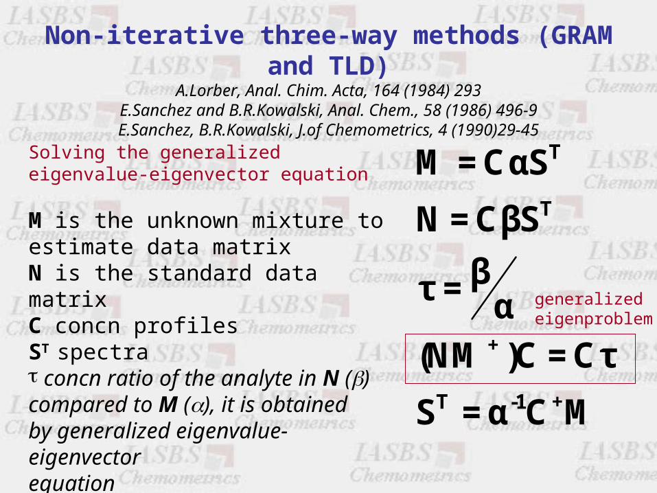
Non-iterative three-way methods (GRAM and TLD)A.Lorber, Anal. Chim. Acta, 164 (1984) 293

E.Sanchez and B.R.Kowalski, Anal. Chem., 58 (1986) 496-9E.Sanchez, B.R.Kowalski, J.of Chemometrics, 4 (1990)29-45

T

T

+

T -1 +

M = CαS

N = CβS

βτ = α

(NM )C = Cτ

S = α C M

Solving the generalized eigenvalue-eigenvector equation

M is the unknown mixture to estimate data matrix N is the standard data matrixC concn profilesST spectra concn ratio of the analyte in N () compared to M (), it is obtainedby generalized eigenvalue-eigenvectorequation

generalized eigenproblem

PARAFAC-ALSR.Bro, Chemolab, (1997) 149-171

Alternating Least Squares Algorithm:

1. Determination of the number of chemical compounds (N) in the original three-way array.

2. Calculation of initial estimates for C and ST.3. Estimation of T, given DT, C and ST.

4. Estimation of C, given DR, ST and T.

5. Estimation of ST, given DC, C and T.

6. Go to 3 until convergence is achieved.

This data decomposition gives the same number of components in the different modes/orders!!

2ˆ(C,S,T) d-dfFind the minimum of

PARAFAC-ALSR.Bro, Chemolab, (1997) 149-171Step 4 of the algorithm (example)

4. Estimation of C, given DR, ST and T.

D

DR

Row-wise augmented data

matrix DR

* * * *

** **

* * * *

*

ST

TALS C

C = DR Z+

Z = T ST

Kronecker product

Tucker-ALSP.M.Kroonenberg and J.DeLeeuw, Psychometrika, 45 (1980) 9

2ˆ(C,S,T,G) d-df

1. Determination of the number of componentsin each order.1. Calculation of initial estimates for C, S and T.2. Estimation of G, given C, S and T.3. Estimation of C, given G, S and T.4. Estimation of ST, given G, C and T.5. Estimation of T, given G, C and ST

6. Go to 3 until convergence is achieved.

This data decomposition allows different umber of components in the different orders!!

Find the minimum of

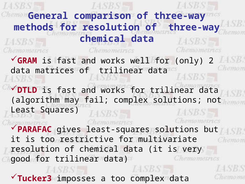
General comparison of three-way methods for resolution of three-way chemical data

GRAM is fast and works well for (only) 2 data matrices of trilinear data

DTLD is fast and works for trilinear data (algorithm may fail; complex solutions; not Least Squares)

PARAFAC gives least-squares solutions but it is too restrictive for multivariate resolution of chemical data (it is very good for trilinear data)

Tucker3 imposses a too complex data structure model for multivariate resolution of usually found chemical data

General comparison of three-way methods for resolution of three-way chemical data

MCR-ALS model is similar to a Tucker2 or a Tucker1 model (depending on the case):

a) it is very flexible and easy to use and interpret

b) only needs one order/mode/direction in common

c) different number of rows are allowed in differnt matrices

d) constraints can be applied for each individual species and matrix

e) it adapts easily to chemical data with a simple bilinear model and constraints;

e) it may assume simple interaction between components (like in Tucker models).

Deviations from trilinearity Mild Medium Strong Array size

PARAFAC

Small PARAFAC2

Medium TUCKER

Large MCR, PCA, SVD,..

Guidelines for selection of resolution methodJournal of Chemometrics, 2001, 15, 749-771

Software

1. N-way toolbox by C. Andersson and R. Bro.http://www.models.kvl.dk/source/nwaytoolbox2. MCR-ALS by R. Tauler and A. de Juan.http://www.ub.es/gesq/mcr/mcr.htm

http://www.models.kvl.dk/source/nwaytoolbox

http://www.models.kvl.dk/source/nwaytoolbox

http://www.ub.es/gesq/mcr/mcr.htm




Lecture 3



data. – Constraints. – Extension of resolution conditions. – Recovery of quantiative information.– Breaking rank deficiencies by matrix augmentation– Feasible bands


Run1Run 2

Run 3 Run 4

Check of trilinear data structure: SVD analysis of concentration profiles

svd of trilinear data

1.5018e-004

1.0421e-004

3.8935e-005

1.7183e-005

1.7569e-020

9.7494e-021

8.5585e-021

5.9053e-021

5.1355e-021

4.5152e-021

0 10 20 30 40 50 600

1

2x 10

-5

0 10 20 30 40 50 600

2

4x 10

-5

0 10 20 30 40 50 600

1

2x 10

-5

0 10 20 30 40 50 600

1

2x 10

-5

Example 1 Four chromatographic runs following a trilinear model

lof % R2

a) Theoretical 1.634 0.99973 (added noise)b) MA-MCR-ALS-tril 1.624 0.99974c) PARAFAC 1.613 0.99974

(small overfitting)

0 10 20 30 40 50 60 70 80 90 1000

0.05

0.1

0.15

0.2

0.25

0.3

0.35

O PARAFAC+ MA-MCR-ALS tril- theoretical

0 20 40 60 80 100 120 140 160 180 2000

0.5

1

1.5

2

2.5

3

O PARAFAC+ MA-MCR-ALS tril- theoretical

Three-way trilinear data: spectra recovery

species TLD (cos) ALS (cos) TLD (sin) ALS (sin)

1 0,9995 0,9999 0,033 0,0107

2 1 1 0,0069 0,0068

3 0,9998 0,9999 0,0221 0,0136

4 0,9999 1 0,0124 0,0086

Trilinear data: quantitative recovery

Species Matrix theoretical TLD ALS

1 2 0,5 0,5 0,5

3 1,2 1,2 1,2

4 0,7 0,7 0,7

2 2 0,8 0,85 0,84

3 0,5 0,48 0,5

4 0,66 0,67 0,67

3 2 1,87 1,85 1,87

3 1,25 1,24 1,25

4 0,62 0,62 0,62

4 2 0,8 0,82 0,81

3 1,2 1,21 1,2

4 0,5 0,5 0,5

Calculation of feasible bands in the simultaneous resolution of several

chromatographic runs (runs 1, 2, 3 and 4)

0 5 10 15 20 25 30 35 40 45 500

0.2

0.4

0.6

0 20 40 60 80 100 120 140 160 180 2000

1

2

3

4

Run 1 Run2 Run 3 Run 4

Matrix augmentation,non-negativity andspectra normalizationconstraints

Calculation of feasible bands in the simoultaneous resolution of several


Matrix augmentation,non-negativity,spectranormalization and selectivity constraints

Totally uniquesolutions are notachieved in thiscase!

0 5 10 15 20 25 30 35 40 45 500

0.1

0.2

0.3

0.4

0.5

0.6

0 20 40 60 80 100 120 140 160 180 2000

1

2

3

4

0 5 10 15 20 25 30 35 40 45 500

0.05

0.1

0.15

0.2

0.25

0.3

0.35

0.4

0.45

0.5

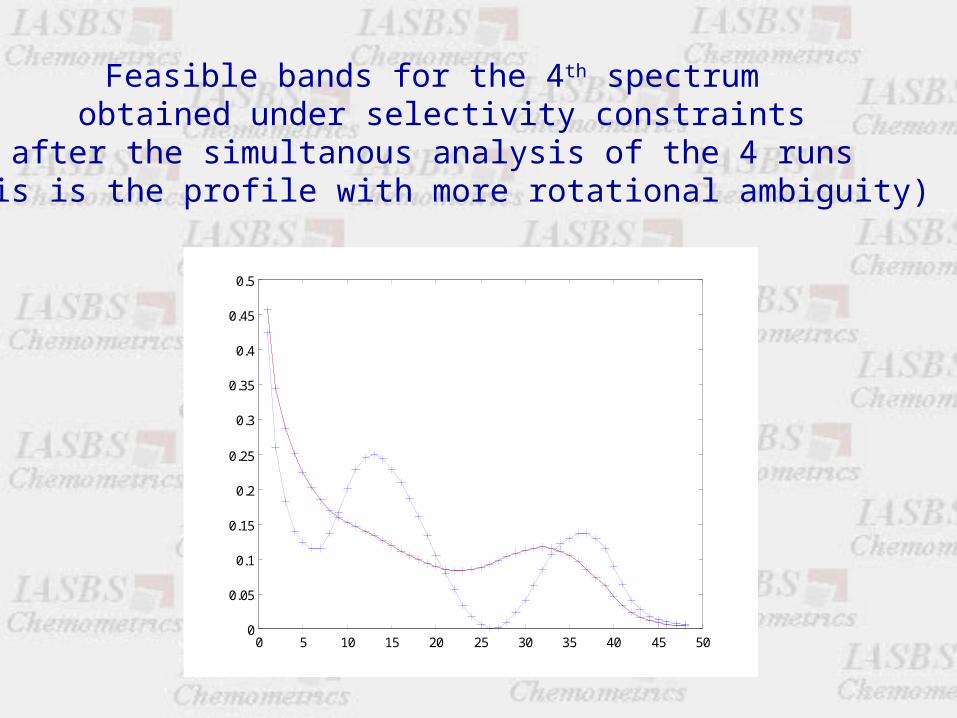
Feasible bands for the 4th spectrum obtained under selectivity constraints

after the simultanous analysis of the 4 runs(this is the profile with more rotational ambiguity)

0 10 20 30 40 50 60 70 80 90 1000

0.05

0.1

0.15

0.2

0.25

0.3

0.35

0 20 40 60 80 100 120 140 160 180 2000

0.5

1

1.5

2

2.5

3

Trilinearitygives unique

solutions!

Calculation of feasible bands in the simoultaneous resolution of several


Matrix augmentation,non-negativity, spectranormalization and trilinearity constraints

4

N

ijk in jn kn ijkn 1

d c s t e

Non-trilinear data

0 50 100 150 2000

0.1

0.2

0.3

0.4

0.5

0.6

0.7

Run1Run 2

Run 3

Run 4

0 50 100 150 2000

0.5

1

1.5

2x 10

-5

0 50 1000

1

2

3

4x 10

Non-trilinear data

0 50 100 150 200

0

0.5

1

1.5

2x 10

-5

The chromatographic profiles of the commoncomponents in every simultaneously analyzed

data matrix are different (in shape and position)

Test of three-way non-trilinear data structure

svd non-trilinear

1.3933e-004

7.5324e-005

3.8957e-005

1.9943e-005

9.3868e-006

7.8565e-006

6.0801e-006

2.2149e-006

1.1052e-006

7.4765e-007

0 10 20 30 40 50 600

1

2x 10

-5

0 10 20 30 40 50 600

1

2x 10

-5

0 10 20 30 40 50 600

1

2x 10

-50 10 20 30 40 50 600

1

2x 10

-5

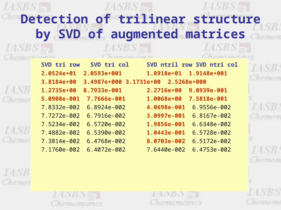
Detection of trilinear structure by SVD of augmented matrices

SVD tri row SVD tri col SVD ntril row SVD ntri col

2.0524e+01 2.0593e+001 1.8918e+01 1.9148e+001

3.8184e+00 3.4987e+000 3.1731e+00 2.5268e+000

1.2735e+00 8.7933e-001 2.2716e+00 9.0939e-001

5.0908e-001 7.7666e-001 1.0068e+00 7.5818e-001

7.8332e-002 6.8924e-002 4.0698e-001 6.9556e-002

7.7272e-002 6.7916e-002 3.0997e-001 6.8167e-002

7.5234e-002 6.5720e-002 1.9856e-001 6.6348e-002

7.4882e-002 6.5390e-002 1.0443e-001 6.5728e-002

7.3814e-002 6.4768e-002 8.0703e-002 6.5172e-002

7.1760e-002 6.4072e-002 7.6440e-002 6.4753e-002

Concentration (elution) profiles: non-trilinear dataIt is very difficult to resolve each chromatographic run individually!

Local rank resolution conditions are now present in run 4

0 20 40 60 80 100 120 140 160 180 2000

0.2

0.4

0.6

0.8

1

1.2

1.4

1.6

1.8

2

Run 1

Run 2

Run 3Run 4

0 20 40 60 80 100 120 140 160 180 2000

1

2

0 20 40 60 80 100 120 140 160 180 2000

1

2

0 20 40 60 80 100 120 140 160 180 2000

0.5

1

1.5

0 20 40 60 80 100 120 140 160 180 2000

0.5

1

1.5

Elution feasible bands: matrix augmentation, non-negative, spectra normalization

and selectivity constraints

blue = no selectivity(feasible bandsno-unimodal)

red = selectivity(unique solutions)

0 20 40 60 80 1000

0.05

0.1

0.15

0.2

0.25

0 20 40 60 80 1000

0.05

0.1

0.15

0.2

0.25

0.3

0.35

0 20 40 60 80 1000

0.05

0.1

0.15

0.2

0.25

0 20 40 60 80 1000

0.1

0.2

0.3

0.4

Spectra feasible bands: matrix augmentation, non-negative, spectra normalization

and selectivity constraints

blue = no selectivity(feasible bands)

red = selectivity(unique solutions)

one of the bounds of feasible bands(no selectivity)is equal to thereal solution

Example 2 Four chromatographic runs not following a trilinear model

lof % R2

a) Theoretical 0.9754 0.99990 (added noise)b) MA-MCR-ALS-tril 17.096 0.97077(the data system is far from trilinear, and impossing trilinearity gives a much worse fit and wrong

shapes of the recovered profiles)

0 20 40 60 80 100 120 140 160 180 2000

0.5

1

1.5

2

2.5

3

0 10 20 30 40 50 60 70 80 90 1000

0.05

0.1

0.15

0.2

0.25

0.3

0.35

+ MA-MCR-ALS tril- theoretical

+ MA-MCR-ALS tril- theoretical


lof % R2

a) Theoretical 0.9754 0.99990 (added noise)b) PARAFAC lof (%) 14.34 0.97941(the data system is far from trilinear, and impossing trilinearity gives a much worse fit and wrong

shapes of the recovered profiles)

0 10 20 30 40 50 60 70 80 90 1000

0.05

0.1

0.15

0.2

0.25

0.3

0.35

0.4

0.45

0.5

0 50 100 150 200 2500

0.5

1

1.5

2

2.5

3

3.5

O PARAFAC- theoretical

O PARAFAC- theoretical

0 20 40 60 80 100 120 140 160 180 2000

0.5

1

1.5

2

2.5

3

3.5

0 10 20 30 40 50 60 70 80 90 1000

0.05

0.1

0.15

0.2

0.25

0.3

0.35


lof % R2

a) Theoretical 0.9754 0.99995 (added noise)b) MA-MCR-ALS-non-tril 0.9959 0.99990

(good MA and local rank conditions for total resolution without ambiguities)

+ MA-MCR-ALS non tril- theoretical

+ MA-MCR-ALS non tril- theoretical

Species TLD ALS (cos) ALS (sin)

1 complex 0,9984 0,0567

2 complex 0,9997 0,0246

3 complex 1 0,008

4 complex 1 0,008

Three-way non-trilinear data: spectra recovery

Non-trilinear data: quantitative recovery

Species Matrix theoretical ALS

1 2 0,61 0,55

3 0,81 0,84

4 0,38 0,39

2 2 1,34 1,39

3 0,34 0,31

4 0,18 0,17

3 2 2,13 2,2

3 1 1,07

4 0,27 0,25

4 2 0,68 0,68

3 0,27 0,26

4 0,4 0,41

Example of Quantiative determinationsDetermination of triphenyltin in sea-water by

excitation-emission matrix fluorescenceand multivariate curve resolution

A method for the determination of triphenyltin (TPhT) in sea-water was proposed:

1) Solid phase exctraction (SPE) of sea-water samples;2) Reaction with a fluorogenic reagent (flavonol in a micellar

medium); 3) Excitation-emission fluorescence measurements (giving an

EEM data matrix);4) MCR-ALS analysis of EEM data matrices5) Quantitation of TPhT

J.Saurina, C.Leal, R.Compañó, M.Granados, R.Tauler and M.D.Prat. Analytica Chimica Acta, 2000, 409, 237-245

Example of Quantiative determinations Determination of triphenyl in sea-water byexcitation-emission matrix fluorescence

and multivariate curve resolution.

Difficulties were:

- low concentrations of TPht ng/l- strong background (fulvic acids) emission- strong reagent emission- lack of selective emission/excitation wavelengths- to have sea-water TPhT standards available

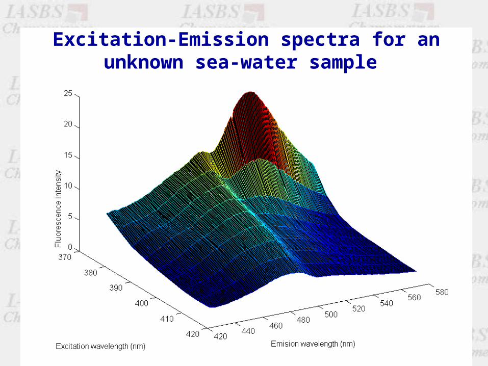
Excitation-Emission spectra for an unknown sea-water sample

U

R

B

S

ex,mex,1

em,1

em,m

em,1

em,n

em,m

em,1

em,m

em,1

=

em,1

em,m

em,1

em,n

em,m

em,1

em,m

em,1

XT

EU

ER

EB

ES

em,1

em,m

em,1

em,n

em,m

em,1

em,m

em,1

ex,mex,1

ex,mex,1

+

YU

YS

YR

YB

U unknown sea water; S TPhT pure standard;R reagent (flavonol); B sea-water background (fulvic acids)

EEM Daug

emission Yaug

excitation XT

noise Eaug

= +

MCR-ALS resolution of EEM data

MCR-ALS resolution of EEM data

Model:[U;S;R;B] =Daug = YaugXT + Eaug

Resolution: (emission) Yaug= Daug (XT)+ Constraints:

- non-negativity(excitation) XT= (Yaug)+Daug - trilinearity

Quantitation:

cU = [Area(y1,U) / Area(y1,S)] cS

450 500 5500

2

4

Emission wavelength (nm)

Rel

ativ

e in

tens

ity

2

1

3

a


450 500 550

Rel

ativ

e in

tens

ity

0

2

4b

1

2

Emission wavelength (nm)450 500 550

0

2

4

Rel

ativ

e in

tens

ity

2

c


450 500 5500

2

4

Rel

ativ

e in

tens

ity

d

3

415400 405 410

0

2

4

Excitation wavelength (nm)

Arb

itra

ry in

tens

ity

e

1

2

3

300305

310315420 460 500 540 580

123456789

Excitation Wavelength (nm)

Emission Wavelength (nm)

Flu

ores

cenc

e In

tens

ity

300305

310315 420 460 500 540 580

0

1

2

3

4

5

ExcitationWavelength (nm)


Flu

ores

cenc

e In

tens

ity

300305

310315 420 460 500 540

1

2

3

4



Flu

ores

cenc

e In

tens

ity

300305

310315 420 460 500 540 580

0

1

2



Flu

ores

cenc

e In

tens

ity

MCR-ALS

(a)

(e)

(d)

(c)

(b)

(f)

MCR-ALS resolution of [U;S;R;B] augmented matrix

a) 3-D plots of the EEM fluorescence of the unknown sample U, standard S, flavonol reagent R and sea-water background B; b) emission spectra for the unknown sea-water sample; c) emission species spectra for the standard; d) emission species spectra for flavonol reagent; e) emission species spectra for sea-watere background; and f) excitation spectra

1 TPhT flavonol complex2 Flavonol reagent3 sea-water background

U

S

R

B

0

0.5

1

1.5

2

2.5

3

0 10 20 30 40 50

Concentration (pg/l)

Resp

onse

Standards

Synthetic

See Water A

See Water B

See Water C

See Water D

See Water E

Plot of the emission profiles areas for TPhT species in standards, synthetic and sea-water samples respect the

analyte concentration

MCR-ALS resolution/quantitation of EEM data

0

5

10

15

20

25

30

35

40

45

0 10 20 30 40 50

Real Concentration (ppt)

Calc

ula

ted

co

ncen

trati

on

(p

pt)

Comparison between 'true' and MCR-ALS calculated TPhT concentrations in sea-water samples

overall prediction errors were always below 13%!

Quantitation: cU = [Area(yU) / Area(yS)] cS

FIGURES OF MERIT IN SECOND ORDERMULTIVARIATE CURVE RESOLUTION

• From MCR-ALS resolution of the pure response profiles of theanalyte in different known and unknown mixures (data matrices),a Calibration Curve is built.

• Figures of merit such as Limit of Detection, Sensitivity, Precisionand Accuracy are calculated from the calibration curve

like in univariate calibration!

J. Saurina*, C. Leal, R. Compañó, M. Granados, M. D. Pratand R.Tauler

0

0.5

1

1.5

2

2.5

3

3.5

0 5 10 15

TPhT concentration (µg / L)

Re

lativ

e A

rea

Approach (a) [U;S2;R] ri = 0.260 ci + 0.014 (r = 0.998)

Approach (b) [U1;U2;U3;U4;U5;U6;U7;U8;U9;U10;U11;U12;S2;R;B]ri = 0.244 ci + 0.201 (r = 0.987)

Building the Calibration Curve and Sensitivity

ri = ai / astd= f(cstd)

Precision bands

0

0.5

1

1.5

2

2.5

3

0 2 4 6 8 10 12

TPhT Concentration (µg / L)

Relat

ive ar

ea

r c± sRt ( 1/m + 1/n + (ri - )2 / (ci - )2)1/2

LOD = + t sR / b ( 1/m + 1/n +

+ ((ri- ) / b)2 / (ci - )2)1/2r c

Limit of detection

(a) and (b) LOD = 0.7 g l-1

1n

rr̂ = s 1

2i

R

n

ii

(a) and (b) sR = 0.0404

Precision:

Accuracy of the method in the prediction of TPhT in real samples

0

10

20

30

40

0 10 20 30 40

Actual Concentration

Cal

cula

ted

C

on

cen

trat

ion

(n

g/L

)

Sea Water A

Sea Water B

Sea Water C

Sea Water D

c

c - c

= 2

i

Samples

1=i

2ii

Samples

1=i 100 x (%) Error

)(

)ˆ(

Error % = 5.5 % for strategy (A)Error % = 12.7 % for strategy (B)

overall prediction error

Solving matrix effects in the analysisof triphenyltin in sea-water samples by three-way

multivariate curve resolution

•Three strategies were compared for the recovery of the analyte response in the sea-water samples: (i) using pure standards (ii) using sea-water standards; and (iii) using the standard addition method

•The combination of standard addition with multivariate curve resolution method improved the accuracy of predictions in the presence of matrix effects.

J.Saurina and R.Tauler, The Analyst, 2000, in press

Standard addition strategy:For each unknown sample, MCR-ALS is applied to the following aug-mented matrices (i.e A4, the same for the other A1, A2, A3, A5 and A6) augmented matrices identification[A4;S2;R;B] => A4 unknown sample [A4SA1;S2;R;B] => A4SA1 = A4 + 0.20 µg l-1 TPhT[A4SA2;S2;R;B] => A4SA2 = A4 + 0.75 µg l-1 TPhT[A4SA3;S2;R;B] => A4SA3 = A4 + 1.05 µg l-1 TPhT[A4SA4;S2;R;B] => A4SA4 = A4 + 1.87 µg l-1 TPhT [A4SA5;S2;R;B] => A4SA5 = A4 + 3.30 µg l-1 TPhT[A4SA6;S2;R;B] => A4SA6 = A4 + 4.52 µg l-1 TPhT[A4SA7;S2;R;B] => A4SA7 = A4 + 7.42 µg l-1 TPhT

S2 EMM response matrix of an standard of TPhTR EMM response matrix of the reagentB EMM response matrix of the background

0

0.5

1

1.5

2

2.5

-20 0 20 40

TPhT concentration(µg / L)

Re

lati

ve

Are

a

Standard addition calibration graph ina sea-water analyte determination

(sea-water sample A4)

-100

-50

0

50

100

A1 A2 A3 A4 A5 A6

Sample Reference

Pre

dic

tio

n E

rro

r (%

)

standards

Pure standards

Sea-water

Standardaddition

Prediction errors in the determination of TPhT in sea-water samplesA1-A6 using MCR-ALS and three calibration approaches:

Recent advances and current research on MCR-ALS method

•Hybrid soft- hard- (grey) bilinear models (kinetic and equilibrium chemicalreactions, profile responses shape...)•Extension to multiway data analysis (PARAFAC, Tucker3 models....)•Multivariate Image Analysis.(MIA)•Weighted Alternating Least Squares (WALS)•Calculation of feasible band boundaries (rotation ambiguity)•Error propagation in MCR-ALS solutions•……•Applications: Bioanalytical: polynucleotides, proteins, u-array...Environmental: contamination sources resolution and apportionemntAnalytical: Hyphenated methods(LC-DAD, LC-MS, GC-MS, FIA-DAD,…), multidimensional spectroscopies (2D-NMR, EEM ,… ON-line spectroscopic monitoring of (bio)chemical processes and reactions......….

New user interface: http://www.ub.es/gesq/mcr/mcr.htmJ. Jaumot,et al., Chemometrics and Intelligent Laboratory Systems, 2005, 76(1) 101-110

Multivariate Resolution in Chemistry Lecture 3 Roma Tauler IIQAB-CSIC, Spain e-mail:...

Documents

Transcript of Multivariate Resolution in Chemistry Lecture 3 Roma Tauler IIQAB-CSIC, Spain e-mail:...