Normal Probability Distributions 1. Section 1 Introduction to Normal Distributions 2.
Upload
eunice-collinsCategory
view
268download
5
Multivariate distributions

The Normal distribution

1.The Normal distribution – parameters and (or 2)
Comment: If = 0 and = 1 the distribution is called the standard normal distribution
0
0.005
0.01
0.015
0.02
0.025
0.03
0 20 40 60 80 100 120
Normal distribution with = 50 and =15
Normal distribution with = 70 and =20
2221
( ) e ,2
x
f x x
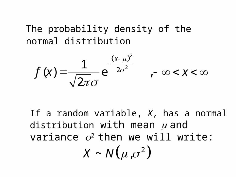
The probability density of the normal distribution
If a random variable, X, has a normal distribution with mean and variance 2 then we will write:
2~ ,X N
The multivariate Normal distribution
Let1
p
x
x
x
= a random vector
Let1
p
= a vector of constants (the mean vector)

Let1
1
p
p p
p pp
= a p × p positive
definite matrix

Definition
The matrix A is positive semi definite if
for all x Ax 0 x
Further the matrix A is positive definite if
only if x Ax 0 x 0

1( ) , , pf x f x x
Suppose that the joint density of the random vector
The random vector, [x1, x2, … xp] is said to have a p-variate normal distribution with mean vector and covariance matrix
We will write:
~ ,px N
11
2/ 2 1/ 2
1e
2
x x
p
x
is:x

Example: the Bivariate Normal distribution
11
21 2 1/ 2
1, e
2
x xf x x
with 1
2
22 1 2
22 22 22 2 2
and

Now
1x x
and
2 2 2 222 12 1 2 1
-1
11 12 1 11 1 2 2
12 22 2 2
, x
x xx
22 12 1 11 1 2 2
12 11 2 2
1,
xx x
x

2 2
22 1 1 12 1 1 2 2 11 2 2
12x x x x
2 22 22 1 1 1 2 1 1 2 2 1 2 2
2 2 21 2
2
1
x x x x
2 2
1 1 1 1 2 2 2 2
1 1 2 2
2
2
1
x x x x

Hence
11
21 2 1/ 2
1, e
2
x xf x x
2 2
1 1 1 1 2 2 2 2
1 1 2 2
1 2 2
2
,1
x x x x
Q x x
1 2
1,
2
21 2
1e
2 1
Q x x
where

Note:
2 2
1 1 1 1 2 2 2 2
1 1 2 2
1 2 2
2
,1
x x x x
Q x x
1 21
,2
1 2 21 2
1, e
2 1
Q x xf x x
is constant when
is constant.
This is true when x1, x2 lie on an ellipse centered at 1, 2 .

x
y
f(x,y)
x
y
f(x,y)
x
y
f(x,y)
The Bivariate Normal Distribution
x
y y y
x x1
2
1 1
2 2
Contour Plots of the Bivariate Normal Distribution
x
y y y
x x1
2
1 1
2 2
Scatter Plots of data from the Bivariate Normal Distribution
1 2 1 2 1 2
1 2 1 2 1 2
1 21 2
1 2

Surface Plots of the bivariate Normal distribution

Contour Plots of the bivariate Normal distribution

Scatter Plots of data from the bivariate Normal distribution
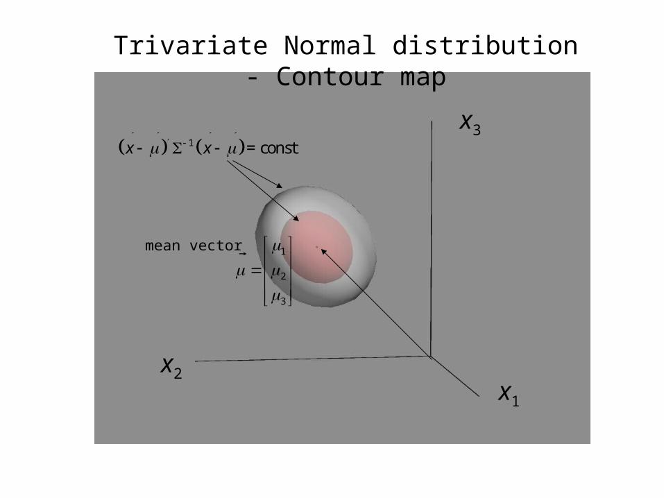
Trivariate Normal distribution - Contour map
x1
x2
x3
mean vector 1
2
3
1 = const x x
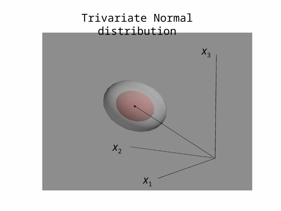
Trivariate Normal distribution
x1
x2
x3

Trivariate Normal distribution
x1
x2
x3

Trivariate Normal distribution
x1
x2
x3

example
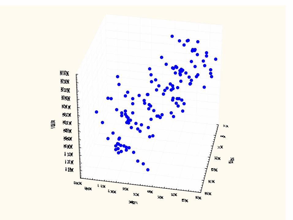
In the following study data was collected for a sample of n = 183 females on the variables
• Age,
• Height (Ht),
• Weight (Wt),
• Birth control pill use (Bpl - 1=no pill, 2=pill)
and the following Blood Chemistry measurements
• Cholesterol (Chl),
• Albumin (Abl),
• Calcium (Ca) and
• Uric Acid (UA). The data are tabulated next page:

The data :Age Ht Wt Bpl Chl Alb Ca UA Age Ht Wt Bpl Chl Alb Ca UA Age Ht Wt Bpl Chl Alb Ca UA
22 67 144 1 200 43 98 54 27 64 120 1 172 43 98 60 37 67 125 2 200 45 99 66 25 62 128 1 243 41 104 33 27 64 180 2 317 37 98 84 37 65 116 1 270 42 100 48 25 68 150 2 50 38 96 30 27 69 137 1 195 46 101 42 37 63 129 2 230 36 91 22 19 64 125 1 158 41 99 47 27 64 125 2 185 36 94 54 38 64 165 1 255 44 102 62 19 67 130 2 255 45 105 83 27 63 125 1 168 42 97 41 38 65 151 2 275 38 94 46 20 64 118 1 210 39 95 40 27 64 124 2 200 40 96 52 39 64 135 1 210 40 95 46 20 64 118 1 210 39 95 40 27 60 140 1 250 36 98 68 39 64 108 2 198 44 90 38 20 65 119 2 192 38 93 50 27 65 155 2 280 42 103 52 39 63 195 1 260 40 108 42 21 60 107 1 246 42 101 52 28 65 108 1 260 48 106 51 39 69 132 2 180 39 94 30 21 65 135 2 245 34 106 48 28 62 110 2 250 44 105 38 39 62 100 1 210 45 91 27 21 63 100 1 208 38 98 54 28 65 120 1 175 48 100 47 39 62 110 2 235 41 99 35 21 64 120 2 260 47 106 38 28 66 113 2 305 41 93 24 40 63 110 1 196 39 97 42 21 67 134 1 204 40 108 34 28 62 135 1 200 43 97 37 40 64 151 2 305 39 99 48 21 67 145 2 192 39 95 49 28 65 160 2 235 42 101 41 40 65 145 1 170 45 100 43 21 63 138 1 280 41 102 41 29 61 142 1 177 39 99 46 40 66 140 2 276 46 100 55 21 64 113 2 230 39 99 38 29 61 115 2 235 45 98 47 40 65 140 1 272 41 91 44 21 63 160 1 215 39 96 39 29 68 155 1 226 38 94 43 40 65 137 2 315 37 96 99 21 64 115 2 225 44 105 44 29 65 118 2 230 44 99 44 40 67 130 1 300 40 106 52 21 68 125 1 165 48 105 28 30 66 143 1 198 45 107 65 40 62 117 2 290 42 99 42 21 62 106 2 200 38 95 40 30 63 110 2 295 45 98 46 41 62 116 1 320 44 111 61 21 68 150 1 220 47 102 75 30 61 99 1 230 43 99 39 41 68 215 2 255 43 105 45 21 64 130 2 255 34 102 40 30 63 132 2 200 37 96 34 41 64 125 1 306 45 98 62 22 62 135 1 263 43 98 47 30 62 125 1 230 46 104 48 41 69 170 2 324 40 99 55 22 62 110 2 173 42 97 37 30 63 110 2 262 33 99 41 42 60 105 1 240 41 101 51 22 57 105 1 170 46 98 45 30 64 135 1 174 40 95 35 42 63 129 2 210 40 100 46 22 64 120 2 290 37 98 59 30 66 112 2 250 44 100 35 43 66 167 1 210 40 100 52 22 64 115 1 263 42 102 47 30 64 160 1 217 35 95 31 43 68 145 2 250 36 98 42 22 59 94 2 220 47 105 46 31 65 125 1 250 43 98 39 43 66 138 1 335 44 105 58 22 67 125 1 200 43 100 44 31 66 120 2 237 34 91 49 43 66 132 2 230 42 98 48 22 62 97 2 192 38 95 43 31 65 115 1 270 41 111 64 43 64 125 1 285 45 105 50 22 58 100 1 247 42 104 52 31 63 110 2 280 44 99 49 43 62 113 2 200 40 93 36 22 66 130 2 175 44 106 58 31 66 123 1 238 37 96 33 43 64 126 1 280 45 106 38 22 60 100 1 155 41 96 45 31 67 136 2 218 38 95 42 43 65 148 2 276 41 105 50 22 60 100 1 155 41 96 45 32 67 132 1 185 39 103 37 55 64 124 1 275 40 98 53 22 65 135 2 215 40 93 43 32 68 203 2 235 38 99 37 55 64 165 2 298 36 100 63 22 60 95 1 200 47 99 34 32 62 155 1 262 37 99 43 44 62 118 1 253 43 94 44 22 67 124 2 247 44 102 45 32 65 126 2 160 41 97 40 44 63 133 2 242 47 104 49 23 63 125 1 220 32 92 42 32 63 125 1 189 40 94 40 45 67 180 1 160 38 97 59 23 64 105 2 207 42 100 40 32 71 170 2 205 37 90 60 45 65 140 2 263 45 107 52 23 63 125 1 266 42 103 47 32 62 120 1 260 43 107 38 46 67 145 2 320 40 101 37 23 63 120 2 240 43 101 39 32 62 145 2 240 45 108 42 46 63 138 1 257 40 90 61 24 68 125 1 195 49 106 52 32 66 140 1 197 44 106 58 46 62 118 2 190 38 95 43 24 64 130 2 250 39 103 46 32 68 133 2 180 32 95 40 46 62 103 1 230 43 102 33 24 64 130 2 250 39 103 46 54 67 140 2 245 39 104 56 46 65 190 2 265 41 108 85 24 65 130 1 225 50 108 39 33 64 115 1 205 47 100 54 47 67 135 1 297 42 100 45 24 65 148 2 200 37 104 49 33 60 118 2 260 38 99 38 47 67 143 2 255 41 100 40 24 64 135 1 180 37 96 49 33 67 137 1 243 41 106 55 47 61 132 1 257 39 96 38 24 71 156 2 240 42 102 51 33 68 130 2 195 40 95 58 47 59 94 2 257 41 103 53 25 62 107 1 330 48 101 53 33 65 130 1 203 44 101 48 48 62 120 1 300 39 94 51 25 67 175 2 175 39 93 51 33 69 138 2 222 40 104 42 48 66 143 2 225 40 100 62 25 66 112 1 205 46 101 33 34 62 112 1 197 37 93 44 48 67 143 1 216 40 96 47 25 63 120 2 235 44 103 40 34 63 125 2 245 38 95 41 48 65 134 2 248 42 102 42 54 67 127 2 260 44 106 57 35 62 115 1 180 40 91 59 48 65 164 1 306 44 100 78 25 67 135 1 295 46 106 47 35 67 125 2 223 40 100 37 48 66 120 2 235 36 97 35 25 67 141 2 230 38 101 52 35 66 138 1 254 39 107 41 48 60 125 1 195 41 95 53 26 66 135 1 240 48 103 51 35 66 140 2 245 39 105 56 48 64 138 2 338 37 100 58 26 64 118 2 238 40 99 46 36 62 135 1 247 34 90 44 49 64 126 1 255 41 102 48 26 65 125 1 198 44 96 43 36 67 120 2 175 46 103 39 49 69 158 2 217 36 106 65 26 65 120 2 196 38 95 43 36 66 112 1 215 43 104 42 50 69 135 1 295 43 105 63 36 65 121 2 270 43 98 35 50 66 140 2 390 46 97 55 52 62 107 2 265 46 104 64 53 65 140 2 220 40 107 46 54 66 158 1 305 42 103 48 54 60 170 2 220 35 88 63

3D Scatterplot Wt,Ht Age

3D Scatterplot Alb, Chl, Bp

Marginal and Conditional distributions

1
2
Let q
p q
xx
x
Theorem: (Marginal distributions for the Multivariate Normal distribution)
11 12
12 22
have p-variate Normal distribution
with mean vector1
2
q
p q
and Covariance matrix
Then the marginal distribution of is qi-variate Normal distribution (q1 = q, q2 = p - q)
iiwith mean vector i
and Covariance matrix
ix
1
2
Let q
p q
xx
x
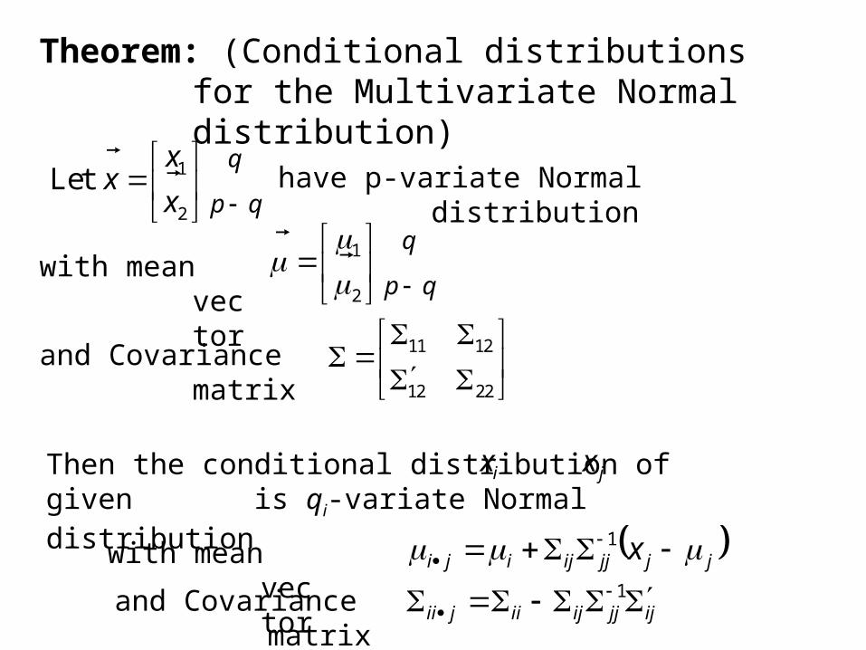
Theorem: (Conditional distributions for the Multivariate Normal distribution)
11 12
12 22
have p-variate Normal distribution
with mean vector1
2
q
p q
and Covariance matrix
Then the conditional distribution of given is qi-variate Normal distribution
with mean vector
and Covariance matrix
ix
jx
jjjjijiji x
1
ijjjijiijii
1
1
2
x
xx
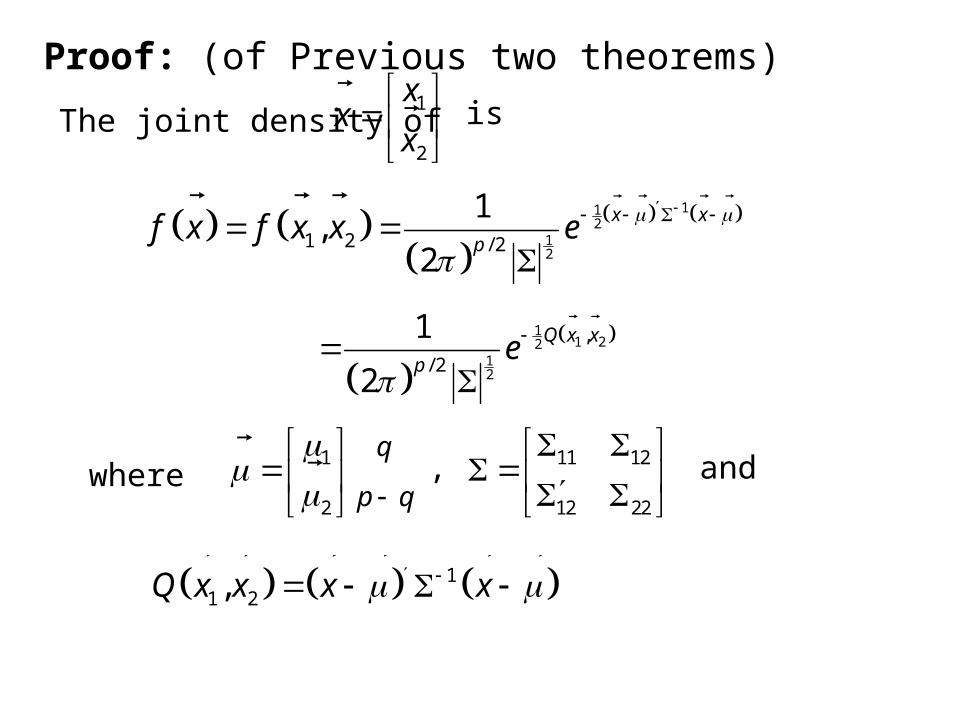
Proof: (of Previous two theorems)
11 12
12 22
is
where1
2
q
p q
,
The joint density of
and
112
12
1 2 / 2
1,
2
x x
pf x f x x e
1
1 2212
,
/ 2
1
2
Q x x
pe
11 2,Q x x x x

-1 11 1211 121
21 2212 22
where,
and
11 2,Q x x x x
11 12
1 11 1 2 2 21 22
2 2
,x
x xx
222 2 2 2x x
11 121 1 1 1 1 1 2 22x x x x
-112 1 1 2111 12 22 12 11 12 =
111 1 1 1 111 11 12 22 12 11 12 12 11
122 1
22 12 11 12

also
,
and
-11 11 1 11 12 22 12 11 12 2 22 x x
11 1 11 1 1x x
111 22 12 11 12
222 2 2 2x x
11 121 1 1 1 1 1 1 1 2 2, 2Q x x x x x x
11 1 11 1 11 12 22 12 11 12 12 11 1 1x x
-112 2 22 12 11 12 2 2 x x

,
-11 12 2 12 11 1 1 22 12 11 12x x
11 2 1 1 11 1 1Hence ,Q x x x x
12 2 12 11 1 1x x
1 1 2 1 2,Q x Q x x
11 1 1 11 1 1where Q x x x
12 1 2 2 2 12 11 1 1and ,Q x x x x
-11 122 12 11 12 2 2 12 11 1 1x x
-12 2x b A x b
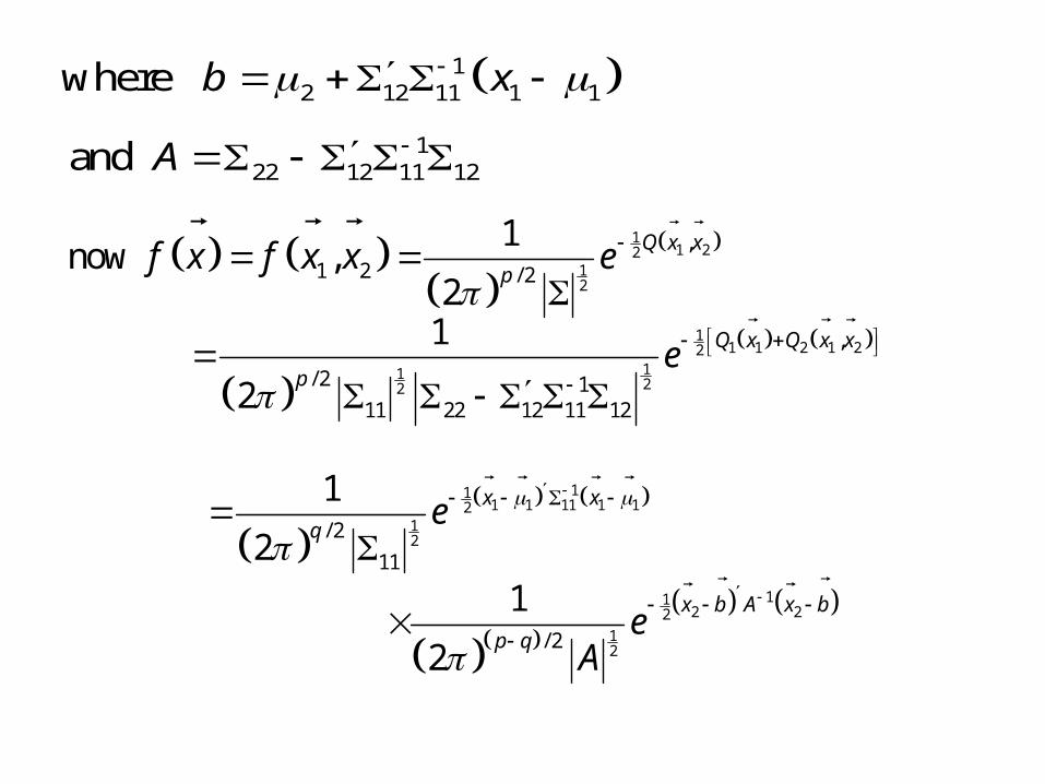
12 12 11 1 1where b x
122 12 11 12and A
11 22
12
,1 2 / 2
1now ,
2
Q x x
pf x f x x e
1
1 1 2 1 221122
,
/ 2 111 22 12 11 12
1
2
Q x Q x x
pe
11
1 1 11 1 1212/ 2
11
1
2
x x
qe
11
2 22
12/ 2
1
2
x b A x b
p qe
A

1 1 1 2 2 1 2 1 , , q pf x f x x dx f x x dx dx
11
1 1 11 1 1212/ 2
11
1
2
x x
qe
11
2 22
12
2/ 2
1
2
x b A x b
p qe dx
A
The marginal distribution of is1 x
11
1 1 11 1 1212/ 2
11
1
2
x x
qe

1 2
2|1 2 11 1
,
f x xf x x
f x
11
2 22
12/ 2
1
2
x b A x b
p qe
A
The conditional distribution of given is:2 x
1 x
12 12 11 1 1where b x
122 12 11 12and A

12 1 22 12 11 12The matrix
is called the matrix of partial variances and covariances.
th
2 1The , element of the matrix i j
1,2....ij q
is called the partial covariance (variance if i = j) between xi and xj given x1, … , xq.
1,2....1,2....
1,2.... 1,2....
ij qij q
ii q jj q
is called the partial correlation between xi and xj given x1, … , xq.
121
111222122
122qij ,,2,1
qjjqii
qijqij
,,2,1,,2,1
,,2,1,,2,1

112 11the matrix
is called the matrix of regression coefficients for predicting xq+1, xq+2, … , xp from x1, … , xq.
12 1 1 2 12 11 1 where x
Mean vector of xq+1, xq+2, … , xp given x1, … , xqis:
jxB12

Example:
10
15 and
6
14
Suppose that
1
2
3
4
x
xx
x
x
Is 4-variate normal with
4 2 4 2
2 17 6 5
4 6 14 6
2 5 6 7

1
10 and
15
The marginal distribution of1
12
xx
x
is bivariate normal with
11
4 2
2 17
1
10
15 and
6
The marginal distribution of1
1 2
3
x
x x
x
is trivariate normal with
11
4 2 4
2 17 6
4 6 14

Find the conditional distribution of
11
2
15
5
xx
x
given
11
4 2
2 17
1 2
10 6 and
15 14
Now
and
32
4
xx
x
22
14 6
6 7
12
4 2
6 5

114 6 4 6 4 2 4 2
6 7 2 5 2 17 6 5
9 3
3 5
121
111222122

112 11
The matrix of regression coefficients for predicting x3, x4 from x1, x2.
14 6 4 2
2 5 2 17
0.875 .250
0.375 .250

6 0.875 0.250 10
14 0.375 0.250 15
6.5
6.5
12 12 11 1
2 1
0.875 15 0.250 5 6.5 7.875
0.375 15 0.250 5 6.5 13.375
5.6250.0375.0
5.6250.0875.0
21
21112 xx
xxx
B

Thus the conditional distribution of
11
2
15
5
xx
x
given
is bivariate Normal with mean vector
And partial covariance matrix
32
4
xx
x
2 1
7.875
13.375
2 1
9 3
3 5
12
12

Using SPSS
Note: The use of another statistical package such as Minitab is similar to using SPSS

The first step is to input the data.
The data is usually contained in some type of file.
1. Text files
2. Excel files
3. Other types of files

After starting the SSPS program the following dialogue box appears:

If you select Opening an existing file and press OK the following dialogue box appears

Once you selected the file and its type

The following dialogue box appears:

If the variable names are in the file ask it to read the names. If you do not specify the Range the program will identify the Range:
Once you “click OK”, two windows will appear

A window containing the output

The other containing the data:

To perform any statistical Analysis select the Analyze menu:

To compute correlations select Correlate then BivariateTo compute partial correlations select Correlate then Partial

for Bivariate correlation the following dialogue appears

Correlations
1.000 .080 .253** .372** -.069 .009 .210**
. .281 .001 .000 .357 .899 .004
183 183 183 183 183 183 183
.080 1.000 .481** -.007 -.013 .147* .106
.281 . .000 .930 .863 .047 .153
183 183 183 183 183 183 183
.253** .481** 1.000 .131 -.235** .072 .291**
.001 .000 . .078 .001 .330 .000
183 183 183 183 183 183 183
.372** -.007 .131 1.000 .075 .269** .294**
.000 .930 .078 . .313 .000 .000
183 183 183 183 183 183 183
-.069 -.013 -.235** .075 1.000 .454** .039
.357 .863 .001 .313 . .000 .603
183 183 183 183 183 183 183
.009 .147* .072 .269** .454** 1.000 .178*
.899 .047 .330 .000 .000 . .016
183 183 183 183 183 183 183
.210** .106 .291** .294** .039 .178* 1.000
.004 .153 .000 .000 .603 .016 .
183 183 183 183 183 183 183
Pearson Correlation
Sig. (2-tailed)
N
Pearson Correlation
Sig. (2-tailed)
N
Pearson Correlation
Sig. (2-tailed)
N
Pearson Correlation
Sig. (2-tailed)
N
Pearson Correlation
Sig. (2-tailed)
N
Pearson Correlation
Sig. (2-tailed)
N
Pearson Correlation
Sig. (2-tailed)
N
AGE
HT
WT
CHL
ALB
CA
UA
AGE HT WT CHL ALB CA UA
Correlation is significant at the 0.01 level (2-tailed).**.
Correlation is significant at the 0.05 level (2-tailed).*.
the output for Bivariate correlation:

for partial correlation the following dialogue appears

- - - P A R T I A L C O R R E L A T I O N C O E F F I C I E N T S - - -Controlling for.. AGE HT WT CHL ALB CA UACHL 1.0000 .1299 .2957 .2338 ( 0) ( 178) ( 178) ( 178) P= . P= .082 P= .000 P= .002ALB .1299 1.0000 .4778 .1226 ( 178) ( 0) ( 178) ( 178) P= .082 P= . P= .000 P= .101CA .2957 .4778 1.0000 .1737 ( 178) ( 178) ( 0) ( 178) P= .000 P= .000 P= . P= .020UA .2338 .1226 .1737 1.0000 ( 178) ( 178) ( 178) ( 0) P= .002 P= .101 P= .020 P= .(Coefficient / (D.F.) / 2-tailed Significance)" . " is printed if a coefficient cannot be computed
the output for partial correlation:

Correlations
1.000 .080 .253** .372** -.069 .009 .210**
. .281 .001 .000 .357 .899 .004
183 183 183 183 183 183 183
.080 1.000 .481** -.007 -.013 .147* .106
.281 . .000 .930 .863 .047 .153
183 183 183 183 183 183 183
.253** .481** 1.000 .131 -.235** .072 .291**
.001 .000 . .078 .001 .330 .000
183 183 183 183 183 183 183
.372** -.007 .131 1.000 .075 .269** .294**
.000 .930 .078 . .313 .000 .000
183 183 183 183 183 183 183
-.069 -.013 -.235** .075 1.000 .454** .039
.357 .863 .001 .313 . .000 .603
183 183 183 183 183 183 183
.009 .147* .072 .269** .454** 1.000 .178*
.899 .047 .330 .000 .000 . .016
183 183 183 183 183 183 183
.210** .106 .291** .294** .039 .178* 1.000
.004 .153 .000 .000 .603 .016 .
183 183 183 183 183 183 183
Pearson Correlation
Sig. (2-tailed)
N
Pearson Correlation
Sig. (2-tailed)
N
Pearson Correlation
Sig. (2-tailed)
N
Pearson Correlation
Sig. (2-tailed)
N
Pearson Correlation
Sig. (2-tailed)
N
Pearson Correlation
Sig. (2-tailed)
N
Pearson Correlation
Sig. (2-tailed)
N
AGE
HT
WT
CHL
ALB
CA
UA
AGE HT WT CHL ALB CA UA
Correlation is significant at the 0.01 level (2-tailed).**.
Correlation is significant at the 0.05 level (2-tailed).*.
Compare these with the bivariate correlation:
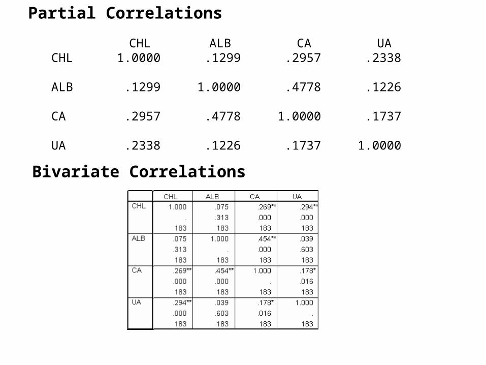
CHL ALB CA UACHL 1.0000 .1299 .2957 .2338 ALB .1299 1.0000 .4778 .1226 CA .2957 .4778 1.0000 .1737 UA .2338 .1226 .1737 1.0000
Partial Correlations
Bivariate Correlations

In the last example the bivariate and partial correlations were roughly in agreement.
This is not necessarily the case in all stuations
An Example:
The following data was collected on the following three variables:
1. Age
2. Calcium Intake in diet (CAI)
3. Bone Mass density (BMI)

The data
Age CAI BMI Age CAI BMI Age CAI BMI
25 75.2 147.7 45 62.5 239.8 65 66.8 298.925 83.6 166.7 45 84.6 257.5 65 53.5 280.625 112.2 254.9 45 107 317.2 65 64.9 287.225 99.8 193 45 82.3 280.3 65 63.8 302.225 93.1 199 45 69.9 232.8 65 52.6 263.325 97.7 202.6 45 100.6 270.5 65 58.8 296.225 103.7 231.7 45 74.1 228.6 65 61.4 294.225 101.8 199.7 45 60.2 231.8 65 59.6 294.325 99.6 182.4 45 94.6 252.5 65 62.9 250.425 94.9 202.8 45 80.7 254.9 65 52 26525 99.6 204.7 45 94.4 266.3 65 60.4 267.625 100.2 206.6 45 73.1 227.9 65 61.2 287.325 116.9 280 45 81.2 245 65 67.4 299.825 97.3 186.9 45 106.1 297.8 65 51.5 273.225 98.8 217.9 45 79.3 217.7 65 60.7 284.225 90.6 198.7 45 85.1 263.9 65 56.3 290.225 101.7 190.4 45 81.9 280.5 65 72.9 306.725 98.6 221.3 45 98.7 281 65 40.3 258.825 93 191.8 45 89.1 275.4 65 47.1 283.625 108.1 216.2 45 71.6 225.2 65 76.9 323.525 78.9 161.3 45 76.9 240.9 65 64.7 303.425 87.1 188.6 45 79.7 252.1 65 59.9 297.935 96 248 55 61.1 238.1 75 37.8 277.935 97 261 55 60.5 250.1 75 43 287.535 94.8 237.5 55 82 285.9 75 33.8 305.935 78.1 225.8 55 70.7 267.1 75 41.5 320.335 93.1 239.7 55 71.9 258.2 75 71.2 353.335 74.3 205.7 55 64.4 245.3 75 58 34535 100.1 255.7 55 66.3 284.9 75 53.4 325.535 95 244.3 55 64.3 281.7 75 37.5 268.535 77 202.3 55 59 249.9 75 41.6 312.135 94.5 231.6 55 83.8 318.1 75 50.9 282.835 108.6 288.2 55 68.9 274.4 75 57.5 346.935 92.4 221.2 55 77.8 266.6 75 51.8 32335 104.3 262 55 63.9 274.9 75 64.9 343.835 87 218.7 55 75.8 277.6 75 44 299.235 88.6 232.3 55 78.8 291.5 75 49.4 313.435 97 252.7 55 82.6 302.8 75 54.4 294.935 85 213.8 55 65.4 270.7 75 53.9 321.335 96.1 232.8 55 59.5 231.3 75 48.7 26235 111.2 288.6 55 54.4 239 75 51.4 325.735 83.9 230.3 55 56.6 247.8 75 49.2 345.535 100.1 248.2 55 55.6 219.9 75 36.5 260.935 91.2 258.6 55 64 249.2 75 61 333.8

Correlations
1.000 -.863** .800**
. .000 .000
132 132 132
-.863** 1.000 -.447**
.000 . .000
132 132 132
.800** -.447** 1.000
.000 .000 .
132 132 132
Pearson Correlation
Sig. (2-tailed)
N
Pearson Correlation
Sig. (2-tailed)
N
Pearson Correlation
Sig. (2-tailed)
N
AGE
CAI
BMI
AGE CAI BMI
Correlation is significant at the 0.01 level (2-tailed).**.
Bivariate correlations

- - - P A R T I A L C O R R E L A T I O N C O E F F I C I E N T S - - - Controlling for.. AGE CAI BMI CAI 1.0000 .8057 ( 0) ( 129) P= . P= .000 BMI .8057 1.0000 ( 129) ( 0) P= .000 P= . (Coefficient / (D.F.) / 2-tailed Significance)
Partial correlations

0
50
100
150
200
250
300
350
400
0 50 100 150
Ca intake
BM
IScatter plot CAI vs BMI (r = -0.447)

0
50
100
150
200
250
300
350
400
0 50 100 150
Ca Intake
BM
I
25 35 45 55 65 75

3D Plot
Age, CAI and BMI


Independence

1 2 and x x
Note: two vectors, , are independent if
11 12
12 22
If is multivariate Normal with mean vector 1
2
and Covariance matrix
Then the conditional distribution of given
12 0
ix
1 2 1 1 2 2, f x x f x f x
jx
is equal to the marginal distribution of ix
1
2
x
xx
Then the two vectors, , are independent if1 2 and x x

x
The components of the vector, , are independent if
ij = 0 for all i and j (i ≠ j )
i. e. is a diagonal matrix

Transformations

Transformations Theorem
Let x1, x2,…, xn denote random variables with joint probability density function
f(x1, x2,…, xn )
Let u1 = h1(x1, x2,…, xn).u2 = h2(x1, x2,…, xn).
un = hn(x1, x2,…, xn).
define an invertible transformation from the x’s to the u’s

Then the joint probability density function of u1, u2,…, un is given by:
11 1
1
, ,, , , ,
, ,n
n nn
d x xg u u f x x
d u u
1, , nf x x J
where
1
1
, ,
, ,n
n
d x xJ
d u u
Jacobian of the transformation
1 1
1
1
detn
n n
n
dx dx
du du
dx dx
du du

ExampleSuppose that u1, u2 are independent with a uniform distribution from 0 to 1
Find the distribution of
Solving for u1 and u2 we get the inverse transformation
1 1 2
2 1 2
2ln sin 2
2ln cos 2
z u u
z u u
2 2 2 21 2 1 2 22ln sin 2 cos 2z z u u u
2 21 22 2
1 2 21 1ln or
2
z zz zu u e
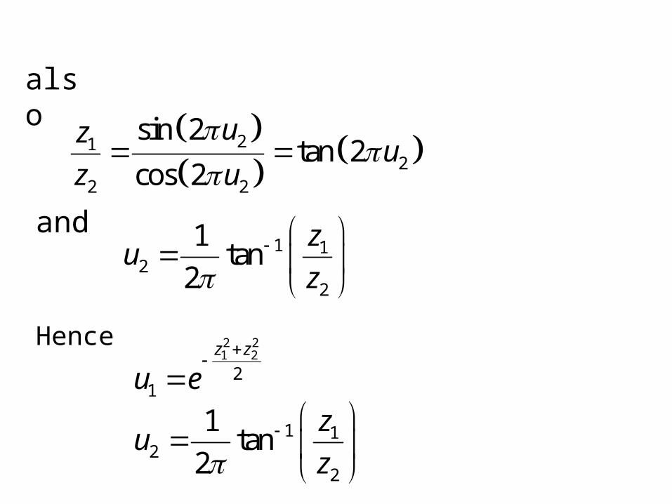
also
Hence
21
22 2
sin 2tan 2
cos 2
uzu
z u
2 21 2
21
z z
u e
and1 1
22
1tan
2
zu
z
1 12
2
1tan
2
zu
z

1 2
1 2
,
,
d u uJ
d z z
The Jacobian of the transformation
1 1
1 2
2 2
1 2
det
du du
dz dz
du du
dz dz
2 2 2 21 2 1 2
2 2
1 2
1 11 1
2 2
1 2
det 1 1tan tan
2 2
z z z zd de e
dz dz
z zd d
z z
dz dz

2 2 2 21 2 1 2
2 21 2
2 12 2 2 21 2 1 2
det 1 1
2 2
z z z z
z e z e
z z
z z z z
2 2 2 21 2 1 22 2
1 12 22 2 2 21 2 1 2
1 1
2 2
z z z zz ze e
z z z z
2 21 2
21
2
z z
e
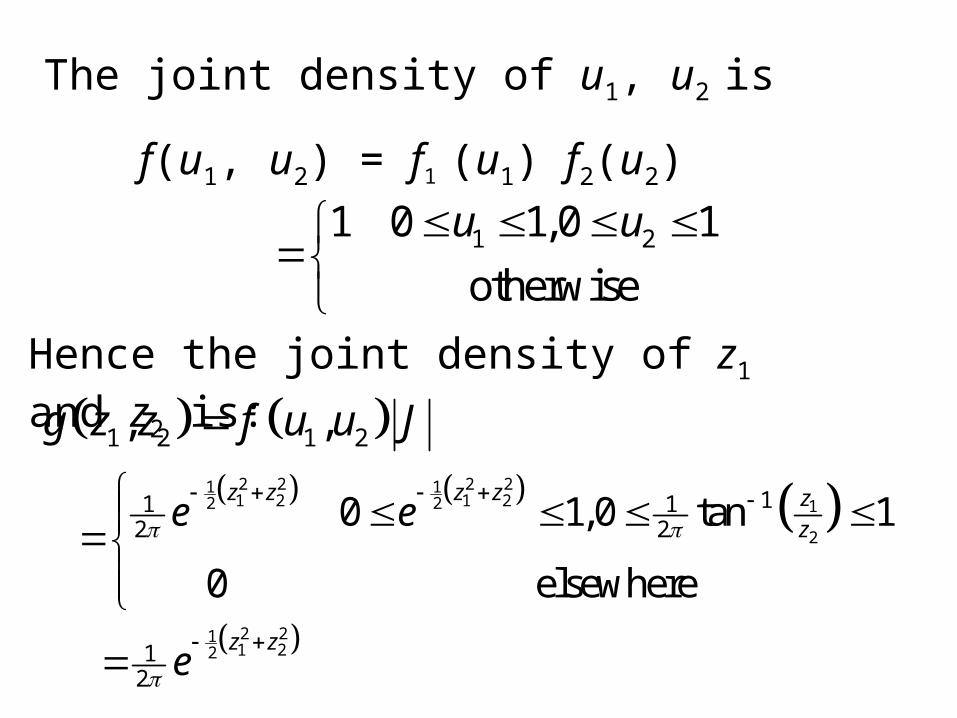
The joint density of u1, u2 is
f(u1, u2) = f1 (u1) f2(u2)
2 2 2 21 11 2 1 22 2 1
2
11 12 20 1,0 tan 1
0 elsewhere
z z z z zze e
1 2 1 2, ,g z z f u u J
Hence the joint density of z1 and z2 is:
1 21 0 1,0 1
otherwise
u u
2 211 221
2
z ze

Thus z1 and z2 are independent Standard normal.
The transformation
1 1 2
2 1 2
2ln sin 2
2ln cos 2
z u u
z u u
is useful for converting uniform RV’s into independent standard normal RV’s

ExampleSuppose that x1, x2 are independent with density functions f1 (x1) and f2(x2)
Find the distribution of
u1 = x1+ x2
u2 = x1 - x2
Solving for x1 and x2 we get the inverse transformation
1 21 2
u ux
1 22 2
u ux

1 2
1 2
,
,
d x xJ
d u u
The Jacobian of the transformation
1 1
1 2
2 2
1 2
det
dx dx
du du
dx dx
du du
1 11 1 1 1 12 2det
1 1 2 2 2 2 2
2 2

The joint density of x1, x2 is
f(x1, x2) = f1 (x1) f2(x2)
Hence the joint density of u1 and u2 is:
1 2 1 21 2
1
2 2 2
u u u uf f
1 2 1 2, ,g u u f x x J
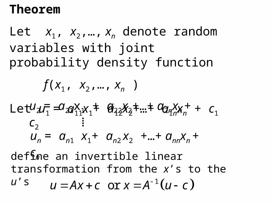
Theorem
Let x1, x2,…, xn denote random variables with joint probability density function
f(x1, x2,…, xn )
Let u1 = a11x1+ a12x2+…+ a1nxn + c1u2 = a21x1 + a22x2+…+ a2nxn + c2
un = an1 x1+ an2 x2 +…+ annxn + cn
define an invertible linear transformation from the x’s to the u’s
1 or u Ax c x A u c
⁞

Then the joint probability density function of u1, u2,…, un is given by:
1 1
1, , , ,n ng u u f x x
A
1 1f A u c
A
where11 1
1
detn
n nn
a a
A
a a
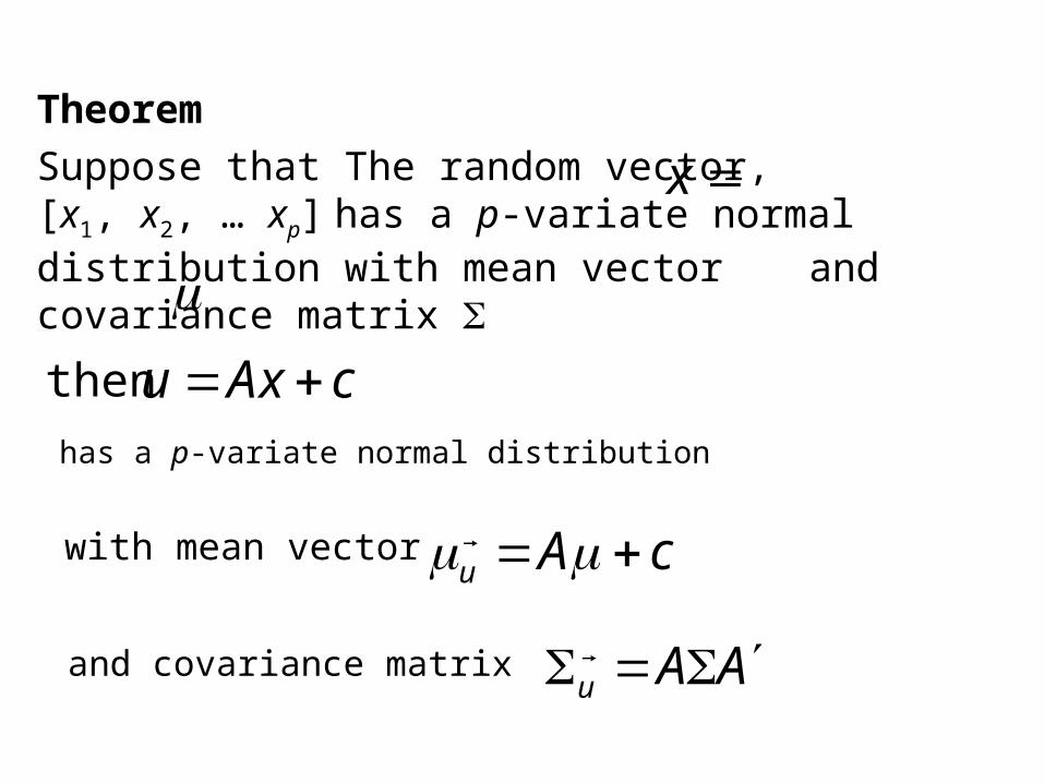
Theorem
Suppose that The random vector, [x1, x2, … xp] has a p-variate normal distribution with mean vector and covariance matrix
x
u A c
then
has a p-variate normal distribution
with mean vector
and covariance matrix u A A
u Ax c

Theorem
Suppose that The random vector, [x1, x2, … xp] has a p-variate normal distribution with mean vector and covariance matrix
x
u A c
then
has a p-variate normal distribution
with mean vector
and covariance matrix u A A
u Ax c

Proof
11
2/ 2 1/ 2
1e
2
x x
pf x
then 1 1 g u f A u c
A
1 1 11
2/ 2 1/ 2
1 1e
2
A u c A u c
p A
1 1 11
2/ 2 1/ 2
1 1e
2
u c A A A u c A
p A

since
1/ 2 A A A A
11
2/ 2 1/ 2
1e
2
u A c A A u A c
pg uA A
1 1 A u c A u c A
Also
1/ 21/ 2 1/ 2= A A A A A and
11 1 1 A A A A and
hence
QED

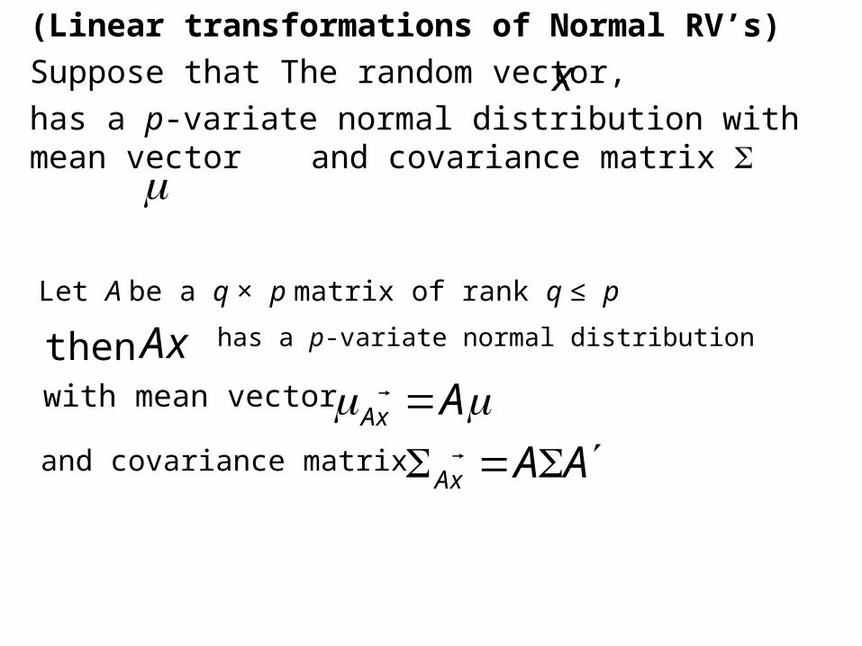
Theorem
(Linear transformations of Normal RV’s)
Suppose that The random vector,
has a p-variate normal distribution with mean vector and covariance matrix
x
Ax A
with mean vector
and covariance matrix Ax A A
then has a p-variate normal distributionAxLet A be a q × p matrix of rank q ≤ p

proof
u
AC
B
then
is invertible.
and covariance matrix
, = u
A A A A BA B
B B A B B
A Axu Cx x
B Bx
Let B be a (p - q) × p matrix so that
AC
B
is p–variate normal with mean vector

AThus the marginal distribution of
and covariance matrix A A
Ax
is q–variate normal with mean vector

Summary – Distribution Theory for Multivariate Normal
• Marginal distribution
• Conditional distribution
2212
1211
2
1
2
1
matrix covariance
r mean vecto with Normal variate- is
ΣΣ
ΣΣΣ
μ
μμ
x
xx
p
111
1
matrix covariancer mean vectowith
Normal variate- is on distributi marginal The
Σμ
x
q
12
1221211
221
22121
21
matrix covariance
andr mean vectowith
Normal variate- is given on distributi lconditiona The
ΣΣΣΣ
μxΣΣμ
xx
q
(Linear transformations of Normal RV’s)
Suppose that The random vector,
has a p-variate normal distribution with mean vector and covariance matrix
x
Ax A
with mean vector
and covariance matrix Ax A A
then has a p-variate normal distributionAxLet A be a q × p matrix of rank q ≤ p

Recall: Definition of eigenvector, eigenvalue
Let A be an n × n matrix
Let and be such thatx
with 0Ax x x
then is called an eigenvalue of A and
and is called an eigenvector of A andx

Thereom If the matrix A is symmetric with distinct eigenvalues, 1, … , n, with corresponding eigenvectors
1 1 1then n n nA x x x x
1, , nx x
Assume 1 i ix x
1 1
1
0
, ,
0n
n n
x
x x
x
PDP
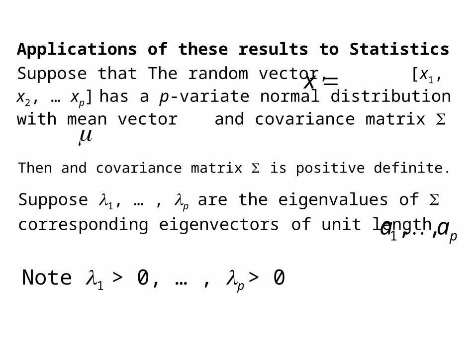
Applications of these results to Statistics
Suppose that The random vector, [x1, x2, … xp] has a p-variate normal distribution with mean vector and covariance matrix
x
Then and covariance matrix is positive definite.
Suppose 1, … , p are the eigenvalues of
corresponding eigenvectors of unit length 1, , pa a
Note 1 > 0, … , p > 0

Let
1, , pP a a
then PDP
1 0
0 n
D
12
1 0
Let
0 p
D
1 12 2then PDP PD D P BB
1 12 2where sometimes denoted by B PD

1 1 12 2 2
1 11 1Note B PD D P D P
1 12 2
11
10
where
10
p
D D
121Note: will be denoted by B

1 12 2hence BB
1 12 2
1 11and BB B B
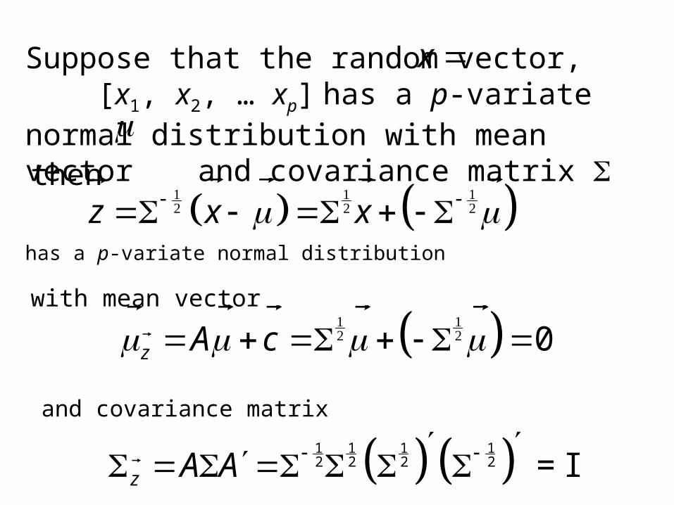
Suppose that the random vector, [x1, x2, … xp] has a p-variate normal distribution with mean vector and covariance matrix
x
0 z A c
then
has a p-variate normal distribution
with mean vector
and covariance matrix
1 1 1 12 2 2 2 = I z A A
z x x

Thus the components of
are independent normal with mean 0 and variance 1.
and
z x
2
1
p
ii
U z z z x x
1x x
Has a 2 distribution with p degrees of freedom