University of Groningen Multivariate statistical modelling ...

Multivariate degradation modelling and its application toreliability testingSari, J.K.
DOI:10.6100/IR637589
Published: 01/01/2008
Document VersionPublisher’s PDF, also known as Version of Record (includes final page, issue and volume numbers)
Please check the document version of this publication:
• A submitted manuscript is the author's version of the article upon submission and before peer-review. There can be important differencesbetween the submitted version and the official published version of record. People interested in the research are advised to contact theauthor for the final version of the publication, or visit the DOI to the publisher's website.• The final author version and the galley proof are versions of the publication after peer review.• The final published version features the final layout of the paper including the volume, issue and page numbers.
Link to publication
General rightsCopyright and moral rights for the publications made accessible in the public portal are retained by the authors and/or other copyright ownersand it is a condition of accessing publications that users recognise and abide by the legal requirements associated with these rights.
• Users may download and print one copy of any publication from the public portal for the purpose of private study or research. • You may not further distribute the material or use it for any profit-making activity or commercial gain • You may freely distribute the URL identifying the publication in the public portal ?
Take down policyIf you believe that this document breaches copyright please contact us providing details, and we will remove access to the work immediatelyand investigate your claim.
Download date: 02. Sep. 2018

MULTIVARIATE DEGRADATION MODELLING AND ITS
APPLICATION TO RELIABILITY TESTING
JOSEPHINE KARTIKA SARI
NATIONAL UNIVERSITY OF SINGAPORE

MULTIVARIATE DEGRADATION MODELLING AND ITS
APPLICATION TO RELIABILITY TESTING
JOSEPHINE KARTIKA SARI (M.Sc., Parahyangan Catholic University, Indonesia)
A THESIS SUBMITTED
FOR THE DEGREE OF DOCTOR OF PHILOSOPHY
DEPARTMENT OF INDUSTRIAL & SYSTEMS ENGINEERING
NATIONAL UNIVERSITY OF SINGAPORE
2007

MULTIVARIATE DEGRADATION MODELLING AND ITS
APPLICATION TO RELIABILITY TESTING
PROEFSCHRIFT
ter verkrijging van de graad van doctor aan de
Technische Universiteit Eindhoven, op gezag van de
Rector Magnificus, prof.dr.ir. C.J. van Duijn, voor een commissie aangewezen door het College voor
Promoties in het openbaar te verdedigen
op vrijdag 3 oktober 2008 om 10.00 uur
door
Josephine Kartika Sari Liem
geboren te Surabaya, Indonesië

Dit proefschrift is goedgekeurd door de promotoren:
prof.dr. M.J. Newby
en
prof.dr.ir. A.C. Brombacher
Copromotor:
L.C. Tang PhD
Copyright © 2008 All rights reserved. No part of this publication may be reproduced, stored in a retrieval system, or transmitted, in any form or by any means, electronic, mechanical, photocopying, recording, or otherwise, without prior written permission of the copyright owner.
CIP-DATA LIBRARY TECHNISCHE UNIVERSITEIT EINDHOVEN Liem, Josephine Kartika Sari Multivariate Degradation Modelling and Its Application to Reliability Testing. -Eindhoven : Technische Universiteit Eindhoven, 2008. – Proefschrift. - ISBN 978-90-386-1387-1. NUR: 804 Keywords: Bivariate and multivariate degradation data / constant-stress degradation test / constant-stress accelerated degradation test / generalized linear model (GLM) / copula functions / LED lighting system Printed by: University printing office, Eindhoven


Acknowledgements
My journey to obtain PhD degree was not only an academic journey but also my personal and
spiritual development journey. During that period, I owed many people for their support,
guidance, and love. Before conveying my thanks to them, I would like to first express my
gratefulness to Lord God, who always accompanies me in my happiness and difficulties, for His
unconditional great love for me.
To do research and study, supervision and advice are needed. The supervision and advice which I
received from my supervisors are intangible not only for my research but also for my personal
development. Therefore, I would like to thank my NUS supervisor, A/P Tang Loon Ching for his
guidance and advice and also because he has introduced me to the quality and reliability area.
From TU/e, I would like to express my thanks to my supervisors Prof. Aarnout C. Brombacher for
his guidance and advice that enable me not only to finish the experiment but also to learn more
things in life (and of course for his training so I could finish my first city-run in reasonable time)
and to Prof. Martin J. Newby for his input and guidance especially in the area of statistics and
modelling. I would also like to express my gratitude for the comments and input from Dr. A. Di
Bucchianico (TU/e), Prof. T. Bedford (University of Strathclyde), and Prof. M. Xie (NUS). In
addition, I would like to thank all the University staff especially Ms. Ow Lai Chun from ISE
department (NUS).
In this project, some experiments were carried out with the support of LedNed BV (my thanks to
Mr. Jurjen Visser from LedNed BV) and the help of a couple of master students. To Yiu Man
Kan and Martin Kools, I would like to thank them for their help and participation in the
experiment.
Putting ideas into good writing is not something easy especially if it is not in our mother-tongue
language. In this case, I would like to thank Jan Rouvroye for his kindness and critics towards my
writing. I thank him also for his help in translating my summary into Dutch and giving useful
suggestions. He also had important role in improving my Dutch.
There is always first time for everything. I experienced my first real interest to research because
of Mr. Tan Hong San who introduced new point of view of research to me. I would also like to
thank Dr. Jaya S. Jayaram, who showed me that statistics is not scary and it could be very
beautiful. They have also showed me that I could praise the Lord by doing my best in research.
i

Not being mentioned first does not mean less important. I want to express my gratefulness to my
parents for their support, love, and especially their prayers. With their love I have more strength
in finishing this difficult journey and more courage to face the future. Thanks also to my other
relatives who have always supported me.
Friends come and go but they are important part of our life and should always be remembered. I
would like to thank Imelda (Neni), Monica, Clement, Tetty, Julia, Vivi, Ridwan, Rubben, Holly,
Alin, Susi, Aunty Jo and Uncle Donald for making me smile most of the time in Singapore.
Thank you also to NUS friends: Henri, Philippe, Ting Ting, Aldy, Andree, Elysabeth, Sugiharcin,
Xin Yan, Darrel, Rob, Wang Qi, and Lin Jun. Thanks to friends from Singa Nglaras group, ex-
Unpar, church and other friends who are not mentioned explicitly here. I was also very lucky to
have very good colleagues in TU/e: Maurits, Kostas, Aylin, Aravindan, Ilse, Joél, Jeroen, Girish,
Christelle, Wim. Special thanks to Hanneke, Lu Yuan, Peter and Valia. Thank you for your
hospitality and friendships.
Being far away from home is difficult. Therefore, we need support from friends. During my stay
in Eindhoven, I owed a lot to Annie and family, Oom Wat Sien and Tante Lana and family, Oom
Teddy and Tante Ursula, Beatrijs and family, Monica, Sri, Irwan, all friends from Eindhoven
Ngakak, IYCE, Javanse dansles, and Oom and Tante at KTM. You have given colour in my life
during my stay in the Netherlands. Special thanks to Fajar, Theresia and Canggih for the sleepless
discussion and movie nights, cooking days, and your love. Thanks for introducing new
perspectives of life to me. Everything surely happens for (at least) a reason. My best wishes for
everybody and I hope all of you have a good journey in pursuing your dreams.
Josephine Kartika Sari Liem
ii

TABLE OF CONTENTS
Acknowledgements i
Table of Contents iii
Summary vii
Sammenvatting ix
List of Tables xi
List of Figures xii
Nomenclatures xvi
Chapter 1: Introduction 1
1.1. Reliability Quantification of Highly Reliable Products 1
1.2. Research Questions 5
1.3. Objectives and Contribution of The Research Work 8
1.4. Organization of the Thesis 9
Chapter 2: Single Performance Characteristic Degradation Test Model 13
2.1. Constant Stress Degradation Test 20
2.2. Accelerated Degradation Test 26
2.2.1. Constant-Stress Accelerated Degradation Test 27
2.2.2. Step-stress Accelerated Degradation Test 30
Chapter 3: Degraded System with Multiple Performance Characteristic 33
3.1. Independent Degradation Model 35
3.2. Dependent Degradation Model 36
Chapter 4: Copula Functions 41
4.1. Basic Principles of Copula Functions 42
4.2. Parametric Copulas 50
4.2.1. Gaussian Copula 51
4.2.2. Student-t Copula 52
iii
4.2.3. Archimedean Copulas 53
Chapter 5: Bivariate Constant-Stress Degradation Test 57
5.1. Bivariate CSDT Model 1 61
5.1.1. Model 1 – Stage 1: Marginal TTF Distribution Estimation 63
5.1.2. Model 1 – Stage 2: System Reliability 70
5.2. Bivariate CSDT Model 2 75
5.2.1. Model 2 – Stage 1: Marginal Degradation Distribution Modelling 76
5.2.2. Model 1 – Stage 2: System Reliability 80
5.3. Bivariate CSDT Model 3 82
5.3.1 Model 3 – Stage 1: Degradation Data and Marginal Reliability
Modelling 83
5.3.2 Model 3 – Stage 2: System Reliability 86
5.4. Numerical Example 86
5.4.1. Model 1 Example 89
5.4.2. Model 2 Example 97
5.4.3. Model 3 Example 103
5.5. Discussion of the Bivariate Models 107
Chapter 6: Multivariate Constant-Stress Degradation Test 111
6.1. Multivariate Copula Functions 113
6.1.1. Multivariate Elliptical Copulas 116
6.1.1.1. Multivariate Gaussian Copula 116
6.1.1.2. Multivariate Student-t Copula 120
6.1.2. Multivariate Archimedean Copulas 121
6.2. Multivariate CSDT Models 126
6.2.1. Multivariate CSDT Model 1 128
6.2.2 Multivariate CSDT Model 2 130
6.2.3 Multivariate CSDT Model 3 131
Chapter 7: Failure Probability Density Function and Reliability Bounds 133
7.1. Failure Probability Density Function Adjustment (Bivariate and
Multivariate CSDT) 135
7.2. Upper and Lower Fréchet-Hoeffding Bounds for Bivariate Degradation Data 138
iv

7.3. Improvement of the Bivariate System Reliability Bounds With Given
Performance Characteristic's Dependency Measurements 140
7.4. Bivariate System Reliability Limits with Given Threshold Value Definition 144
7.5. Numerical Example 148
7.6. Discussion on System PDF Adjustment and Bivariate System Reliability
Bounds and Limits 152
Chapter 8: Bivariate Constant-Stress Accelerated Degradation Test 157
8.1. Basic Principles of Constant-Stress Accelerated Life Test 160
8.2. Basic Principles of Constant-Stress Accelerated Degradation Test 162
8.3. Bivariate CSADT Model 167
8.3.1. Bivariate CSADT Model 1 167
8.3.2. Bivariate CSADT Model 2 170
8.3.3. Bivariate CSADT Model 3 172
8.4. Discussion on Bivariate CSADT Models 173
Chapter 9: Implementation to LED Test Data 177
9.1. LED Lamp 178
9.2. Test Design and Data Collection 179
9.2.1. Bivariate CSDT Data Collection 184
9.2.2. Multivariate CSDT Data Collection 185
9.2.3. Bivariate CSADT Data Collection 186
9.3. Modelling and Analysis 187
9.3.1. Bivariate CSDT Modelling and Analysis 187
9.3.1.1. LED case study: Bivariate CSDT Model 1 189
9.3.1.2. LED case study: Bivariate CSDT Model 2 197
9.3.1.3. LED case study: Bivariate CSDT Model 3 203
9.3.1.4. Bivariate CSDT Discussion 207
9.3.2. Multivariate CSDT Modelling and Analysis 208
9.3.3. Bivariate CSADT Modelling and Analysis 215
9.3.3.1. LED case study: Bivariate CSADT Model 1 217
9.3.3.2. LED case study: Bivariate CSADT Model 2 222
9.3.3.3. LED case study: Bivariate CSADT Model 3 225
9.4. Discussion on the LED Lighting System Test Result 228
v

Chapter 10: Conclusion and Future Research Suggestion 233
10.1. Conclusion 234
10.2. Suggestion for Future Research 236
References 239 Appendix A 250
Appendix B 252
Appendix C 257
Curriculum Vitae 275
vi

Multivariate Degradation Modelling and Its Application to Reliability Testing
Summary
The combination of increased demands on quality and reliability in parallel with the continuous
influx of new technology increases the difficulties in product development and testing processes,
especially when only, due to the “newness” of the technology involved and/or high quality level
of a product very little life time data is available for reliability analysis. In the case addressed in
this thesis, solid state lighting systems, it is expected that the dominant class of failure
mechanisms is of a gradual (and not of a catastrophic) nature where the underlying degradation
model is more complicated to model and test than a traditional life test.
These difficulties are structurally related to the growth and the continuous influx of new
technology. However, there is sometimes a huge social pressure that pushes the application of
new technology. The lighting industry, which is addressed in this thesis, is one of the examples
where there is influx of new technology, which is not fully mature, and pressure to apply the
technology because of social and environmental issues. Other side effect of the influx of new
technology may appear in the form of bivariate or multivariate failure mechanisms.
Motivated by the before mentioned challenges, four research questions are raised. The first three
research questions focus on finding alternative reliability quantification models/methods for bi-
/multi-variate constant-stress degradation test data and for bivariate constant-stress accelerated
degradation test data. This was done with the assumption that the failure mechanisms are not
independent. Generalized linear model and copula functions are utilized as a basis to develop the
proposed models and analysis methods. Aspects such as system failure time distribution function
and reliability bounds and limits are also studied for bivariate degradation data. Despite some
shortcomings of the approach described in this thesis, the capability of the approach is clearly
vii

shown. The strength of the proposed models is on their flexibility on modelling bivariate and
multivariate degradation data with more relaxed assumptions, i.e. independency between the
failure mechanisms is not required.
The fourth research question is dealing with the application of the proposed models to actual
experimental data. A number of case studies performed using LED lights, demonstrate the
application of the proposed models to actual experimental data. These and the analysis results
show the capability of the proposed models and also give some insights in the reliability related
issues in the LED lighting industry. This information will be useful not only to the
engineer/designer but also to the decision maker in this industry.
It can be concluded that this research opens the way for a structured programme of research into
multivariate failure behaviour especially on degraded failures, with a high potential to assess
system reliability including in the situation of a high influx of technology. In addition, some
suggestions to improve the proposed bi-/multi-variate degradation models and study in the area of
LED lighting industry are given.
viii

Samenvatting
De combinatie van verhoogde eisen aan kwaliteit en bedrijfszekerheid in parallel met de
continue instroom van nieuwe technologie vergroot de problemen rondom
productontwikkeling en test processen, in het bijzonder als vanwege de "nieuwheid" van
de technologie en/of het hoge kwaliteitsniveau van een product, onvoldoende levensduur
data beschikbaar zijn voor analyse van bedrijfszekerheid. In de toepassing behandeld in
dit proefschrift, zogenoemd 'solid state lighting', wordt verwacht dat de dominante klasse
van faal mechanismes gradueel is (niet catastrofaal), waardoor het onderliggende
degradatiemodel en de bijbehorende test meer gecompliceerd zijn dan de traditionele
levensduur test.
Deze problemen hangen structureel samen met de groei en continue instroom van nieuwe
technologie. Vanuit de samenleving is er echter soms een grote druk die de toepassing van
nieuwe technologie drijft. De verlichtingsindustrie, het toepassingsgebied van dit
proefschrift, is een van de voorbeelden waar sprake is van een instroom van nieuwe, nog
niet uitgerijpt technologie, en waar vanwege sociale en milieu gerelateerde redenen sprake
is van druk om deze snel toe te passen. Een zijeffect van de instroom van nieuwe
technologie kan optreden in de vorm van bivariate of multivariate faalmechanismes.
Op basis van het voorgaande zijn vier onderzoeksvragen opgesteld. De drie eerste vragen
zijn gericht op het vinden van alternatieve kwantitatieve
bedrijfszekerheidsmodellen/methodes voor bi-/multivariate constante belasting degradatie
test data en voor bivariate constante belasting versnelde degradatie test data. Dit wordt
gedaan onder de aanname dat de faalmechanismes niet onafhankelijk zijn. 'Generalised
ix

linear models' en 'copula' functies.zijn gebruikt als basis voor de voorgestelde modellen en
analyse methodes. Aspecten zoals systeem faaltijd distributie functie en randvoorwaarden
en limieten voor bedrijfszekerheid voor bivariate degradatie data zijn ook bestudeerd.
Ondanks sommige tekortkomingen in de aanpak beschreven in dit proefschrift, wordt de
geschiktheid van de aanpak gedemonstreerd. De kracht van de voorgestelde modellen zit
in de flexibiliteit van het modelleren van bivariate en multivariate degradatie data onder
minder strikte voorwaarden i.e. onafhankelijkheid van faalmechanismes is niet vereist.
De vierde onderzoeksvraag betreft de toepassing van de voorgestelde modellen op reële
experimentele data. Een aantal case studies uitgevoerd met LED lampen demonstreert de
toepasbaarheid van de voorgestelde modellen op actuele experimentele data. Deze en de
analyse resultaten geven ook inzicht in de bedrijfszekerheid gerelateerde problemen in de
LED verlichtingsindustrie. De resultaten zijn niet alleen buikbaar voor de ontwerpers,
maar ook voor de managers in deze industrie.
Er kan worden geconcludeerd dat dit onderzoek de weg opent voor een gestructureerd
onderzoeksprogramma naar multivariate faalgedrag, met een groot potentieel voor het
bepalen van systeem bedrijfszekerheid speciaal in de situatie van hoge instroom van
nieuwe technologie. Daarnaast geeft dit proefschrift suggesties voor verbetering van de
voorgestelde bi-/multivariate degradatie modellen en voor onderzoek op het gebied van
LED verlichting.
x

List of Tables
Table 5.1 Fatigue crack (inch) data adapted from Bogdanoff and Kozin (1985) 88
Table 5.2 Transformed fatigue crack degradation accumulation (%) data 89
Table 5.3 Regression parameters estimation result of Model 1 92
Table 5.4 TTF data and prediction (in million cycles) 93
Table 5.5 Marginal TTF distribution parameters 93
Table 5.6 Cumulative crack percentage compared to the initial measurement (%) 98
Table 5.7 Estimated marginal degradation distribution parameters of fatigue crack data Model 2 (t in million cycles) 100
Table 5.8 Estimated GLM components of Model 3 (t in million cycles) 104
Table 7.1 Integration result of the fatigue-crack data for bivariate CSDT Model 1 149
Table 7.2 Marginal TTFs (Inverse Gaussian) distribution parameters 151
Table 9.1 Fixed-effect estimated parameter bivariate CSDT Model 1 193
Table 9.2 Predicted TTF data (hours) with critical value 50% 194
Table 9.3 Predicted TTF distribution parameter and copula parameter 194
Table 9.4 Result of stage-1 bivariate CSDT Model 2 199
Table 9.5 The results of stage-1 bivariate CSDT Model 3 204
Table 9.6 The results of stage-1 multivariate CSDT Model 1 for PC 3 and 4 212
Table 9.7 Predicted TTF data (hours) of performance characteristic 3 and 4 with critical value 50% 212
Table 9.8 The results of stage 1 bivariate CSADT Model 1 218
Table 9.9 Predicted TTFs data (hours): critical value 50%, CSADT Model 1 218
Table 9.10 The results of stage 1 bivariate CSADT Model 2 223
Table 9.11 The results of stage-1 bivariate CSADT Model 3 226
xi

List of Figures
Figure 2.1 Roller-coaster curve 15
Figure 5.1 Marginal performance characteristic’s degradation path and the threshold value 59
Figure 5.2 Crack locations of the system/product that represents the two performance characteristics 87
Figure 5.3a 1st performance characteristic transformed accumulative percentage degradation data 90
Figure 5.3b 2nd performance characteristic transformed accumulative percentage degradation data 90
Figure 5.4 Marginal PDF of the bivariate fatigue crack analysis (PDF 1 and PDF 2) and real TTF readings (PDF 1–TTF and PDF 2–TTF) Model 1 scenario 1 95
Figure 5.5 Marginal reliability curves calculated from estimated TTF data (PC 1 and PC 2) and real TTF readings (PC 1 – TTF and PC 2 – TTF) Model 1 scenario 1 95
Figure 5.6 System reliability with independent and dependent assumption (Frank copula – TTF parameter) and from real TTF readings using Frank copula (TTF-Frank copula), Model 1 scenario 1 95
Figure 5.7 Marginal PDF of fatigue crack data Model 1 scenario 2 96
Figure 5.8 Marginal reliability fatigue crack data Model 1 scenario 2 96
Figure 5.9 System reliability fatigue crack data Model 1 scenario 2 96
Figure 5.10a Performance characteristic 1 cumulative percentage degradation data 99
Figure 5.10b Performance characteristic 2 cumulative percentage degradation data 99
Figure 5.11 Marginal PDF fatigue crack data Model 2 scenario 1 101
Figure 5.12 Marginal reliability fatigue crack data Model 2 scenario 1 101
Figure 5.13 System reliability with independent and dependent assumption (Dependent Model 1) and from real TTF readings using Frank copula (From TTF data) Model 2 scenario 1 101
Figure 5.14 Marginal PDF fatigue crack data Model 2 scenario 2 102
Figure 5.15 Marginal reliability fatigue crack data Model 2 scenario 2 102
Figure 5.16 System reliability Model fatigue crack data 2 scenario 2 102
Figure 5.17 Marginal PDF fatigue crack data Model 3 scenario 1 105
Figure 5.18 Marginal Reliability fatigue crack data Model 3 scenario 1 105
xii

Figure 5.19 System reliability fatigue crack data Model 3 scenario 1 105
Figure 5.20 Marginal PDF fatigue crack data Model 3 scenario 2 106
Figure 5.21 Marginal reliability fatigue crack data Model 3 scenario 2 106
Figure 5.22 System reliability fatigue crack data Model 3 scenario 2 106
Figure 7.1a Unadjusted system PDF of fatigue-crack example:bivariate CSDT Model 1 136
Figure 7.1b Contour of unadjusted system PDF in figure 7.1a. The concerned system PDF is the diagonal line only (same t for both failure mechanisms) 136
Figure 7.2 Adjusted system PDF of fatigue-crack data using bivariate CSDT Model 1 149
Figure 7.3 Marginal reliability functions and reliability limits of the bivariate degradation data (bivariate CSDT Model 1) 152
Figure 7.4 System reliability bounds and limits for fatigue-crack data Model 1 failure scenario 1 152
Figure 7.5 Adjusted system PDF related to the system reliability limits: fatigue-crack data Model 1 scenario 1 155
Figure 9.1 High power white LED light bulb experiment set up 180
Figure 9.2 Placement of the LED tube lights inside the temperature chamber 182
Figure 9.3 Schema of the dark box for LED tubular light measurement (Kan, 2007) 182
Figure 9.4 The front side of the measurement box 183
Figure 9.5 The measurement box from the side with the laptop to read the measurement 183
Figure 9.6.a Performance characteristic 1 cumulative degradation curve at 25°C 189
Figure 9.6.b Performance characteristic 2 cumulative degradation curve at 25°C 189
Figure 9.7.a PDF of the predicted bivariate TTF for Normal marginal degradation data (Model 1) 195
Figure 9.7.b PDF of the predicted bivariate TTF for Inverse Gaussian marginal degradation data (Model 1) 195
Figure 9.8.a Bivariate LED system reliability Model 1 (Normal marginal degradation data)196
Figure 9.8.b Bivariate LED system reliability Model 1 (Inverse Gaussian marginal degradation data) 196
Figure 9.9.a Bivariate LED hazard rate Model 1 (Normal marginal degradation data) 197
Figure 9.9.b Bivariate LED hazard rate Model 1 (Inverse Gaussian marginal degradation data) 197 Figure 9.10.a PDF of the TTF for Normal marginal degradation data (bivariate CSDT Model 2) 200
xiii

Figure 9.10.b PDF of the TTF for Inverse Gaussian marginal degradation data (bivariate CSDT Model 2) 200
Figure 9.11 Bivariate LED system reliability Model 2 (Normal marginal degradation data)201
Figure 9.12 Bivariate LED system reliability Model 2 (combined marginal performance characteristics distribution assumptions) 201
Figure 9.13 Hazard rate bivariate CSDT Model 2 (Normal marginal degradation data) 202
Figure 9.14 Hazard rate bivariate CSDT Model 2 (Inverse Gaussian marginal degradation data) 202
Figure 9.15 Hazard rate bivariate CSDT Model 2 (combined marginal degradation distribution assumptions) 202
Figure 9.16.a PDF of the TTF for Normal marginal degradation data (bivariate CSDT Model 3) 204
Figure 9.16.b PDF of the TTF for Inverse Gaussian marginal degradation data (bivariate CSDT Model 3) 204
Figure 9.17.a Bivariate LED system reliability Model 3 (Normal marginal degradation data)206
Figure 9.17.b Bivariate LED system reliability Model 3 (Inverse Gaussian marginal degradation data) 206
Figure 9.18.a Hazard rate bivariate CSDT Model 3 (Normal marginal degradation data) 207
Figure 9.18.b. Hazard rate bivariate CSDT Model 3 (Inverse Gaussian marginal degradation data) 207
Figure 9.19.a Performance characteristic 3 cumulative degradation curve at 25°C 210
Figure 9.19.b Performance characteristic 4 cumulative degradation curve at 25°C 210
Figure 9.20 System reliability of multivariate degraded system 214
Figure 9.21 Marginal PDF of the TTF for performance characteristics 3 and 4 214
Figure 9.22 Joint PDF of the multivariate degraded system 214
Figure 9.23 Hazard rate of the multivariate degraded system 215
Figure 9.24.a Performance characteristic 1 cumulative degradation curve at 25°C (low stress level) 216
Figure 9.24.b Performance characteristic 2 cumulative degradation curve at 25°C (low stress level) 216
Figure 9.25.a Performance characteristic 1 cumulative degradation curve at 55°C (high stress level) 216
Figure 9.25.b Performance characteristic 2 cumulative degradation curve at 55°C (high stress level) 217
xiv
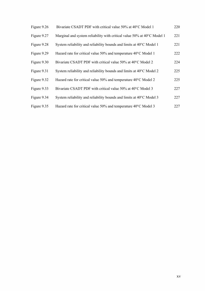
Figure 9.26 Bivariate CSADT PDF with critical value 50% at 40°C Model 1 220
Figure 9.27 Marginal and system reliability with critical value 50% at 40°C Model 1 221
Figure 9.28 System reliability and reliability bounds and limits at 40°C Model 1 221
Figure 9.29 Hazard rate for critical value 50% and temperature 40°C Model 1 222
Figure 9.30 Bivariate CSADT PDF with critical value 50% at 40°C Model 2 224
Figure 9.31 System reliability and reliability bounds and limits at 40°C Model 2 225
Figure 9.32 Hazard rate for critical value 50% and temperature 40°C Model 2 225
Figure 9.33 Bivariate CSADT PDF with critical value 50% at 40°C Model 3 227
Figure 9.34 System reliability and reliability bounds and limits at 40°C Model 3 227
Figure 9.35 Hazard rate for critical value 50% and temperature 40°C Model 3 227
xv

Nomenclatures
β Regression parameter matrix
Γ “Working” correlation matrix
δC Diagonal section of copula
Cρ Spearman rho
Cτ Kendall’s tau
ALT Accelerated Life Test
ARMA Auto-Regressive Moving Average
c Threshold value
Cθ Copula function with copula parameter θ
C(θ Survival copula with copula parameter θ
CDF, F Cumulative distribution function
CSADT Constant-stress Accelerated Degradation Test
CSDT Constant-stress Degradation Test
GLM Generalized Linear Model
GLMM Generalized Linear Mixed-effect Model
h Number of parameters of a distribution function
h(x) Hazard function
( )sh θ1− Inverse of life characteristics ( )sθ
H Joint distribution function
i Index of sample unit, i = 1, 2, …, m
IFM Inference function of marginal
j Index of measurement times, j = 1, 2, …, n
k Index of performance characteristic, k = 1, 2, …, p
LED Light-emitting diode
LDB Lifetime distribution based
M Upper distribution bound
MTTF Mean time to failure
OLS Ordinary least-squares
PA Population average
xvi

PC Performance characteristic
PDF, f(x), f(t) Probability distribution function
PDP Product development process
PSADT Progressive-stress Accelerated Degradation Test
R(x), R(t) Reliability at time x or t respectively
s Stress level
SS Subject specific
SSADT Step-stress Accelerated Degradation Test
SSE Sum of squares error
SSL Solid state lighting
t Measurement time
Tij Standard deviation function of ith sample at jth measurement time
T Standard deviation matrix
TTF Time-to-failure
TTM Time-to-market
u, v CDF of the marginal performance characteristics
U Marginal degradation distribution parameter
V Variance matrix
W Lower distribution bound
WLS Weighted least squares
X Design (controlled variables) matrix
Y Degradation measurement
Z Design (mixed-effect) matrix
xvii


Chapter One
Introduction
1.1 Reliability Quantification of Highly Reliable Products
In this globalization era, companies and manufacturers face increasing pressures. They need
to offer better and cheaper products to consumers while they also have to at least maintain the
quality of the product and profit of the company to stay competitive. There are four business
drivers which need attention for the company to stay competitive (Lu et.al. (1999),
Brombacher (2000)), which are: function, quality, time and cost. From the four business
drivers, it can be seen that companies face conflicting demands to stay competitive and have to
implement the correct strategy to survive.
Reducing the time-to-market (TTM) of a product has been one of the strategies adopted by
many companies to stay competitive. By reducing TTM, companies may gain some
advantages such as: higher possibility to gain more revenue and shorter breakeven time, longer
sales life of the product, higher possibility to attract consumers before other competitors enter
the competition and to increase the market share (Pawar et al., 1994). However, it does not
1

Chapter 1 Introduction mean that the quality of the product can be compromised. In this case, the pressure faced by
the manufacturers is increased because not only they have to reduce the product development
process (PDP) time, but they also have to ensure that the quality of the product reaches the
quality standard.
To add more pressure to the manufacturers, nowadays other dimension of quality has also
been considered by consumers. This additional dimension is time. Consumers’ demands of
product quality nowadays do not stop on its quality at the time the consumers receive the
product but also during a period of time which is also known as the “life” of the product. By
entering time dimension into quality, manufacturers have to consider an additional
specification of product known as reliability. The combination of quality and reliability
aspects increases the difficulties of product development and testing processes which usually
have limited budget and time.
These pressures are added by the increase of the influx of new technology. The availability of
the new technology is not always accompanied by the readiness of the manufacturers to do
mass production and market the new technology as a reliable product. This is because the new
technology may not be mature enough to be adopted by consumers. However, there is
sometimes a huge social pressure that pushes the application of new technology. For example,
the increase of public attention to environmental issues drives many governments to promote
energy savings and reduction of hazardous wastage from the use and production of consumer
products. This gives pressures to the manufacturers to develop and market new technology
that is environmental friendly. Lighting industry, addressed more explicitly later in this thesis,
is one of the examples where there is influx of new technology, which is not fully mature, and
pressure to apply the technology because of social and environmental issues. Light-emitting
diode (LED) which has been considered as a lighting source because of its long life time and
energy efficiency is one of the examples. Since its implementation as solid state lighting
2

Chapter 1 Introduction
(SSL) is relatively new and there is pressure to replace the other more commercially available
lighting sources because of energy efficiency and hazardous material content issues, it is
important to study the performance of the LED lamps in certain conditions (Narendran et.al.,
2004). Reliability is one of the aspects that need to be studied in the implementation of LED
as SSL. Unfortunately, since the product is still new and the influx of technology is high, the
task to quantify the quality and reliability of the new product becomes more difficult because
there are still a lot of unknown factors. Besides the difficulty to assess the product, time and
cost of product development and testing needed can be increased, while the actual time and
cost available are limited.
With all those pressures mentioned above, product quality and reliability cannot be
compromised. The manufacturers have to ensure that their product achieve at least the
minimum standard. Reliability of a product has been receiving increasing attention also
because of the popularity of warranty policy. Nelson (1990) has noted the big effect of
product reliability to the quality and competitiveness of the product. That is why many
manufacturers set quite some budget to improve and evaluate their product in the context of
and related to product reliability. Unfortunately, product reliability assessment has become
more difficult to conduct with the increase of the quality, complexity, and new technology
influx of the product.
In general, product reliability evaluation is strongly related to the product's failure mechanisms
and failure data. However, with the increase of the quality of modern products, the sufficient
failure data that is used to evaluate product reliability may be difficult to obtain because some
products may demonstrate minimal or no failures during a life test. In this case, other test
strategy (i.e. degradation test), in which the product's characteristics related to certain failure
mechanisms are observed instead of the product's catastrophic failures data, is needed to
gather necessary information for product reliability evaluation. On the other hand, the
increase of the complexity of a product means that there is a possibility that multiple failure
3

Chapter 1 Introduction mechanisms may be found in a product. Since the failure mechanisms are of a product, they
may have dependency to each other in a way or another because it is operated in a certain
environmental/operational condition and the product's components share several common
factors.
These difficulties motivate the study on how to quantify reliability of a highly reliable product
or system from a degradation test data. The use of degradation test has increased the
reliability quantification difficulties because degradation data modelling is more complicated
than failure time data modelling. However, degradation test may give “more credible and
precise reliability estimates” compared to the failure test (Meeker et.al., 1998) and it is needed
because of the possible difficulty to obtain sufficient failure data. The degree of this
modelling difficulty is added by the possible existence of more than one dependent failure
mechanisms in a product/system. Consequently, alternative modelling and analysis method
are needed to estimate product/system reliability because the commonly used models and
method might not be sufficient. Therefore, this research is conducted in order to give some
contribution to the quantitative reliability evaluation of a highly reliable product/system with
more than one failure mechanism. These problems are very relevant with the reliability
assessment of LED lamps. In general, it is assumed that LED lamp will have one main
function which is as a lighting source. The commonly assumed failure mechanism of the LED
lamp is the degradation of its light output. However, there are other (multiple) aspects of the
implementation of the LED lamps such as the change of the colour produced by the lamps
during their life time, possible unknown failure mechanisms of the lamps because of the
uncertainty of how the new LED technology will behave, and the arrangement of the lamps in
a system that can lead to different needs of reliability assessment. Because of these reasons,
bivariate or multivariate reliability analysis of LED lamps system from degradation data is
needed. And since this area is relatively new compared to the reliability assessment from data
gathered from a life test and univariate degradation test, there are a lot of possible issues that
4

Chapter 1 Introduction
need to be discussed. Therefore, certain boundary is needed to define the research questions
that will be the guideline of this study. These research questions will be found in the next sub-
chapter.
1.2. Research Questions
In the frame work of reliability quantification of highly reliable product/system, some research
questions are presented. In this thesis, the effort to answer these research questions will be
presented. The research questions are as follows.
Question 1:
“How to quantify the reliability of a product/system which has two degraded
performance characteristics with each performance characteristic leading to
a failure mechanism of the system. These degraded characteristics may not
be independent and may follow different distribution function.”
For this first research question, two degradation test procedures will be considered, which are
constant-stress degradation test (CSDT) and constant-stress accelerated degradation test
(CSADT). In CSDT, the samples are tested under the operational condition/stress(es). While
in CSADT, the samples are tested under several different test condition/stress(es) levels. At
each stress(es) level of the CSADT, a group of sample is allocated for the test. Because two
degradation test procedures are considered in relation to the first research question, it will be
re-defined into two sub-research questions as follows.
Question 1a:
“How to quantify the reliability of a product/system which has two degraded
performance characteristics with each performance characteristic leading to
a failure mechanism of the system. These degraded characteristics may not
5

Chapter 1 Introduction
be independent and may follow different distribution function. The bivariate
degradation data is obtained from a constant-stress degradation test.”
Question 1b:
“How to quantify the reliability of a product/system which has two degraded
performance characteristics with each performance characteristic leading to
a failure mechanism of the system. These degraded characteristics may not
be independent and may follow different distribution function. The bivariate
degradation data is obtained from a constant-stress accelerated degradation
test.”
As the natural extension of research question 1 (especially question 1a) is the quantification of
reliability of a product/system with multivariate degraded performance characteristic. This is
formulated as research question 2.
Question 2:
“How to quantify the reliability of a product/system which has multivariate
degraded performance characteristic with each performance characteristic
leading to a failure mechanism of the system. These degraded
characteristics may not be independent and may follow different distribution
functions. The multivariate degradation data is obtained from a constant-
stress degradation test.”
In quantifying reliability of a bivariate/multivariate degraded system, some issues may be
emerged as consequences of the problem, modelling and estimation methods. Two of the
possible issues are failure probability distribution estimation of the system and bounds and
limits of the system’s reliability estimate. However, since the discussion of multivariate
6

Chapter 1 Introduction
degraded system needs more information and further study, the next research question will be
focused on bivariate degraded system. Then, the third research question can be formulated as
follows.
Question 3:
“How to obtain the bivariate degraded system’s failure probability
distribution, reliability bounds and reliability limits.”
In this thesis, the possible alternative solutions for these three research questions will be
explored, studied and proposed. The proposed models will offer some possible alternative
solutions and directions for future and further research in this area.
Proposed models and methods should be implemented to the real data. In view of the
increasing public attention on environmental issues especially climate change and global
warming, LED lamp is chosen to be the product that will be tested. According to the report of
Energy Information Administration (2007), lighting gives quite big contribution in energy use
in residential, offices and other purposes. Therefore, there are many attempts to develop
energy efficient lighting sources while minimizing the hazardous wastage from the lighting
sources. Development of LED as a lighting source is an example of this attempt and it is
necessary to demonstrate the quality and reliability of this new technology. Therefore, LED
lamps testing was planned to demonstrate the implementation of the proposed models. For
this purpose, degradation tests on some types of light-emitting diode (LED) lamps were
planned and performed. The data gathered from the tests were analyzed using the proposed
models which are the alternative solutions that will be proposed to answer the research
questions 1-3. This will generate the last research question, which can be formulated as
follows.
7

Chapter 1 Introduction Question 4:
“How to demonstrate the proposed models which are the answers of
research question 1-3 to an actual relevant test case (i.e. LED lamps) to
evaluate/assess the reliability of bivariate/multivariate degraded (LED
lighting) system.”
1.3. Objectives and Contribution of the Research Work
Based on the motivation of this research and four research questions that have been presented
in the previous sub-chapters, the objectives which are related to the contribution of this
research work can be concluded.
The first objective of this research is to explore and present the possible models for reliability
quantification of highly reliable product/system. The product/system that is considered here is
the product/system which has more than one performance characteristic that characterize the
failure mechanisms of the product/system. The effort to satisfy this objective will lead to
some contributions of this research which are:
1. Alternative bivariate degradation models that can be used to model bivariate failure
mechanism from CSDT and CSADT data and evaluate the system reliability with more
flexible assumptions, i.e. different marginal degradation distribution function and
dependent failure mechanisms,
2. Alternative multivariate degradation models that can be used to model multivariate failure
mechanism from CSDT data and evaluate the system reliability with more flexible
assumptions, i.e. different marginal degradation distribution function and dependent
failure mechanisms,
8

Chapter 1 Introduction
3. Alternative procedure and methods to estimate the failure probability distribution and
system reliability bounds and limits for bivariate degraded system, which will be useful for
further system assessment and uncertainty analysis.
The second objective of this research is to demonstrate the implementation of the proposed
models to analyze systems/products from a relevant actual test data. In order to realize this
objective, some tests have been planned and conducted on two types of LED lamps which are
arranged in a certain system. The effort to fulfil this objective leads to the fourth contribution
of this research which is the reliability assessment of LED lamps system based on the real test
data. This will not only gives illustration on how the proposed models can be used to assess
actual experiment data but also adds the understanding of reliability and failure behaviour of
certain types of LED lamps which are used and arranged in certain lighting system. With the
big uncertainty of the reliability and failure behaviour of LED lighting system because of the
influx of new LED technology and huge social pressure to apply this technology, the answer to
research question 4 will add new possible alternative in assessing LED lighting system and
gives input for future development of LED as lighting system.
1.4. Organization of the Thesis
This thesis will be organized as follows. Literature review of the degradation models for
single performance characteristic degradation test models will be presented in chapter 2, where
summary of the published research is given. This will give illustration of the possible
extension and/or modification that may be useful for exploring possible models for bi-/multi-
variate degradation models.
The discussion on the few available literatures on the topic of bi-/multi-variate degradation
models is presented in chapter 3. The discussion will include both independent and dependent
failure mechanisms assumptions. The gap of the previous study in bi-/multi-variate models
9

Chapter 1 Introduction will be highlighted here. It is followed by the discussion of the possible functions that can be
incorporated in the proposed models to assess reliability of bi-/multi-variate degraded system
in chapter 4.
Then, this potential functions will be embedded in the proposed models to analyze the
reliability of bivariate degraded system in chapter 5. Three possible models are proposed and
implemented to the widely-used fatigue-crack data to demonstrate the use of the models.
Some comparisons on the proposed bivariate degradation models are also presented in this
chapter.
The extension of the proposed bivariate models to the multivariate models is presented in
chapter 6. The discussion of the multivariate models are restricted to the use of several
possible copula functions because of the need of further study on the topic of multivariate
copulas. Nevertheless, the proposed multivariate models provide alternatives to the analysis of
the system reliability of multivariate degraded system with dependent failure mechanisms
assumption.
In chapter 7, additional issues are discussed. These issues are estimation of the failure
probability distribution and reliability bounds and limits of the system which are useful for the
system and uncertainty analysis. However, this discussion is limited to the bivariate degraded
system. Its extension to the multivariate degraded system is suggested for further research
work.
After discussing models to analyze data from CSDT in chapter 4, proposed models and
analysis method for bivariate degraded system tested using CSADT is presented in chapter 8.
This discussion is offered because in some cases, sufficient data may not be obtained during
CSDT and a CSADT is needed.
10

Chapter 1 Introduction
In chapter 9, case studies of LED lamps system are presented. The data originated from an
actual experiment project. The implementation of the proposed models gives some insights on
the observed system. The results of this chapter will be discussed in chapter 10 in which some
conclusion drawn from the calculation in chapter 9 will be presented in relation with the
assessment of the LED lighting systems considered in this thesis. Additional suggestion and
possible use of the analysis result to improve the development of LED technology as more
efficient and more environmental friendly lighting sources will be given in this chapter.
The last chapter will provide brief summary and conclusion of the thesis and suggestion for
possible further research work.
11


Chapter Two
Single Performance Characteristic Degradation Test Model
One of the important aspects of a product is the quality of the product. By including time
dimension into the quality aspect, consumers' demands of a product also include the quality of
the product during the "life" of the product. This is also known as reliability of the product.
To achieve necessary quality and reliability standards of their products, manufacturers need to
allocate necessary budget and time in the product development process (PDP). The attention
to product reliability has also been increasing because of the popularity of warranty policy.
Therefore, in a PDP, assessment and prediction of the product reliability are needed not only
for design purposes but also for further risk management analysis. Unfortunately, it has
become more difficult to conduct product reliability assessment and prediction because of the
increase of the quality, complexity of the product, and influx of new technology.
In order to discuss reliability quantification, definition of reliability will first be presented.
One of the commonly used definitions of reliability is [O’Connor, Practical Reliability
Engineering, 2002]:
13

Chapter 2 Single Performance Characteristic Degradation Test Model
“The probability that an item will perform a required function without failure under stated
conditions for a stated period of time.”
Therefore, as concluded by Meeker and Escobar (2004), the inclusion of time component is
the major difference between quality and reliability. Reliability can be evaluated
quantitatively and qualitatively. The focus of this thesis is the quantitative aspect of the
reliability. The question is how to quantify reliability of a product. From the definition of
reliability stated above, there is probability involved in the equation. The reliability of a
product thus, can be defined as a probability. Therefore, it is obvious that in order to assess
reliability of a product, statistical knowledge is very important. Meeker and Escobar (2004)
also highlight that statistics has started to give big contribution on reliability improvement
recently.
There are some definitions that are usually used in quantifying reliability of products. The
first one is cumulative distribution function (CDF) which is denoted by:
F(x) = P(X≤ x) = (2.1) ( )∫x
dxxf0
where X is the time-to-failure (TTF) and f(x) is the probability density function (PDF) of the
TTF. The CDF of a product gives the probability that a product will fail before or by time x.
Since F(x) is a probability then F(x) will take value 0 ≤ F(x) ≤ 1.
The second quantifier which is used frequently in reliability mathematics is called reliability or
survival function. The reliability function of a product is the probability that a product will
survive at least until time x. The notation can be written as:
R(x) = P(X > x) = 1 – F(x) (2.2)
14

Chapter 2 Single Performance Characteristic Degradation Test Model
Another measurement which is commonly used is the hazard rate or hazard function. The
hazard function is a conditional probability that a product will fail during (x + dx) given it
survives until time x. So, the hazard function can be written as:
h(x) = ( )( )
( )( )1
f x f xR x F
=− x
(2.3)
This hazard function can be used to describe phases in a non-repairable product’s life, for
example as described in a roller-coaster curve. The roller-coaster curve, which can be
regarded as a development of the classic bathtub curve, gives the big picture of the hazard rate
of non-repairable product during its lifetime. Overall, the roller-coaster curve, which is
introduced by Wong and Lindstrom (1988), has four phases. A description of the roller-
coaster curve can be found in Figure 2.1.
Figure 2.1 Roller-coaster curve
h(t)
This curve is valid only to describe the hazard rate of a population e.g. if all products from one
factory are studied. It should be noted however, that there are examples where the population
rates decreases while some individual rates increase. This comes from the heterogeneity in the
population. The randomness (unexplained heterogeneity) that modifies the hazard rate of an
individual(s) compared to its population is known as frailty (Hougaard, 1995). However,
t
Phase 1 Phase 4
Phase 2 Phase 3
15

Chapter 2 Single Performance Characteristic Degradation Test Model
frailty will not be discussed in this thesis and it will be assumed that the population behaviour
also represents individual behaviour.
Phase one of the roller-coaster curve describes the period of early failure. In this period,
failures caused by severe flaws in the production process and failures categorized as early
failures can be found. Usually, a burn-in procedure is conducted to screen the product from
these kinds of failures before the product is sent to the market. Phase one of the roller-coaster
curve usually reflects a decreasing hazard rate.
Phase two of the roller-coaster curve is usually identified by the hump(s) in the curve. These
humps occur because of the freak/weak sub-populations of the product. Freak/weak
population is a population that can be viewed as having a potential of early aging. Therefore,
items in this sub-population are items that have flaws but not severe enough to initiate early
failures, and will start showing aging effect near their early life. This will increase the
population hazard rate in the second phase of the roller-coaster curve.
Phase three deals with hazard rate of the population after the weak sub-populations disappear
or almost disappear from the population. This phase can be considered as the random hazard
rate of the main population.
The fourth phase of the curve presents illustration of the wear-out process of the main
population. In this phase, an increasing hazard rate is expected. The freak/weak population
will not be found again since they may have failed during the early part of the product’s life.
In order to assess product reliability or identify the four phases of product failures using
Equations (2.1)–(2.3), TTF of the product plays an important role. Therefore TTF data is
needed to do a reliability assessment. One way to collect the product TTF is via a life test.
16

Chapter 2 Single Performance Characteristic Degradation Test Model
Usually, a life test is performed under specified test conditions and test procedures. During
the test, failure data are collected to be analyzed using statistical tools.
Ideally, a life test should be conducted in the conditions as similar as possible with the use
conditions. However, a highly reliable product tested under use condition may need a very
long test time to obtain a sufficient failure data. Manufacturers cannot afford a very long test
time because of the shorter PDP time. For the highly reliable products, the TTF data collected
during a life test may only provides early failure or may be early wear-out phase(s) data of the
product. Therefore, the strategy commonly used to obtain failure data in a shorter time frame
is by conducting an accelerated life test (ALT). In ALT procedure, usually a product is tested
under higher stress levels than the use conditions to motivate early failures. The analysis
results of the failure data then need to be extrapolated to give estimation of the reliability
characteristics in use conditions. However, since an extrapolation is involved and sometimes
the stress-life relationship is not well understood, the reliability characteristics at use
conditions cannot be obtained precisely. An extensive review of accelerated testing can be
found in a book by Wayne Nelson (1990).
With higher reliability of a product and short PDP time available which leads to relatively
shorter testing time available, even ALT may not give enough failure data to assess and
predict the product reliability especially at Phases 3 and 4 of the roller-coaster curve. Some
systems (for example LED lamps) may also have degradation failures as their main failure
mechanisms instead of catastrophic failures. In these cases, other test and reliability
assessment strategies are needed. An alternative to a life test is a degradation test.
Degradation test can be done if there is at least a performance characteristic (PC) of the
product that can be monitored and measured. This PC should be the one whose degradation
leads to failure (Meeker and Escobar, 1998). In this case the product’s failure can be classified
as gradual failure where the product is considered fail when its PC degraded more beyond its
critical performance level.
17
Chapter 2 Single Performance Characteristic Degradation Test Model
Basically in a degradation test, the performance characteristic(s) is (are) monitored over time.
Then the data gathered from the test can be used to evaluate the possible degradation trend(s)
of the product. This trend then can be used to assess the reliability characteristics of the
product. In this way, we do not need to obtain many failure time data. The test result will not
give the lifetime distribution of the product directly, but it can give some insights of the
degradation mechanism, which can be evaluated to obtain the prediction of the product’s life.
Because of the nature of the test, degradation test can be used to identify the reliability
characteristics of products when aging (wear-out) happens. This has also been noticed and
utilized by J.A. van den Bogaard (2005) to answer manufacturing companies’ needs to
optimize product lifecycle. In his work, information from dynamic degradation model and
analysis is used to solve companies’ problem in optimizing their product lifecycle. This is one
of the many examples of the implementation of degradation test to improve a product and
facilitate the company’s effort to stay competitive.
There are some advantages of degradation test over life test as discussed by Meeker et.al.
(1998) in their paper:
1. Degradation test can provide more reliability information than life test when there are very
few failure data obtained,
2. The degradation data gathered may allow us to directly model the failure mechanism.
This, as stated by Meeker et.al. (1998) will give us “more credible and precise reliability
estimates”.
These support the conclusion of Lu et.al. (1996) in their paper in which they compare the TTF
distribution obtained using failure time data analysis versus degradation data analysis. It
should be noted that degradation data modelling is more complicated than failure time data
modelling since there are more unknown factors such as the PC’s distribution function, the
18

Chapter 2 Single Performance Characteristic Degradation Test Model
degradation path of the PC, the dependency between measurements of a PC (i.e. serial-
correlation), the dependency between PCs (in the case of multiple PC), predicted TTF, and
distribution function of the predicted TTF. There are also stronger assumptions needed in the
degradation analysis than in life test analysis. However, Lu et.al. (1996) pointed that
degradation analysis is more robust than failure time analysis when used to estimate
probability beyond the range of the data.
In general, the degradation test data analysis procedure is:
1. Plan the test method (stress level(s), sample size, inspection time, etc.),
2. Select randomly some specimens to be tested,
3. Execute the test and collect the degradation data,
4. Fit the data to a model and obtain the model parameters,
5. Estimate the reliability characteristics. If there is no closed-form available, simulation
method can be used.
Looking at the general outline of degradation test and analysis, some of the complexities of
degradation test modelling and analysis can be concluded. Examples of the complexity are:
how to choose the suitable model for the degradation path, which distribution function should
be chosen to describe the degradation parameters (in the case of parametric model), how to
translate the degradation data to reliability characteristics such as mean time to failure (MTTF)
and TTF distribution, how to model the data if there are more than 1 failure mechanism, etc.
The possibility of the need to assess more than one set of PC degradation in a product may
arise because of the complexity or possible multiple failure mechanisms of a system. Product
complexity may be caused by the multiple aspects of new technology used in a product. This
may motivate the existence of multiple PC. Other situation that can generate the increase of
the number of the PC is the way the product is arranged/designed as a system. The reliability
quantification of product/system with multiple PC (with each PC can be associated to a failure
19

Chapter 2 Single Performance Characteristic Degradation Test Model
mechanism) is the main topic of this thesis and will be discussed in the next chapters. In this
chapter, single PC degradation model will be discussed.
Even though published references in degradation data modelling and analysis are not as
extensive as life test modelling and analysis, it can be seen that the number of references in
degradation modelling and analysis especially for single PC is growing. These include
modelling of the degradation path data for constant stress degradation test (CSDT), estimation
of the degradation parameters, modelling of accelerated degradation test (ADT), and optimum
or near-optimum planning of degradation test. The summary of single PC degradation data
model will be presented in the next sub-chapters and will provide illustration of the past and
recent development in this area and also basic ideas of possible approaches to model reliability
of a degraded system with multiple PC which is the focus of this thesis.
The next sub-chapter will discuss the development in the class of CSDT. CSDT is used when
PC degradation data observed during a test at operational condition is seen to be sufficient to
assess the product reliability. If CSDT cannot provide sufficient data for product reliability
assessment, an accelerated test is performed. This test is called accelerated degradation test
(ADT). Similar to the ALT, ADT is carried out to obtain more data in shorter test time with
possibly harsher test condition. In the second sub-chapter some development in the class of
ADT will be presented.
2.1. Constant Stress Degradation Test
A CSDT is usually performed by testing a number of random samples at operational
conditions. The PC (Yij) of the samples is observed at pre-specified measurement times during
the test. If there are m sample units (i = 1,...,m), and for each sample unit there are ni number
of measurements (j = 1,...,ni), then at the end of the test, pairs of measurement time-PC
20

Chapter 2 Single Performance Characteristic Degradation Test Model
observation are collected , ( )1 1,i it y ( )2 2,i it y , ..., ( ),i iin int y . A common practice of the
degradation data modelling is to use these pairs of data to model the degradation path. The
predicted degradation path will then be used to predict the TTF of the samples. This
information is used to estimate the failure time distribution function and reliability function of
the product.
Oliveira and Colosimo (2004) discuss comparison of three statistical methods that are
commonly used to estimate the TTF distribution function (i.e. the CDF) of the product with
single PC. The three methods are namely approximation method, analytical method and
numerical method. The approximation method is used when the degradation path is relatively
simple and there is enough data to estimate the degradation path parameters. Since the
degradation path is relatively simple and therefore for each sample the predicted failure time
can be estimated relatively easy, these predicted TTF can be used to estimate the TTF
distribution with assumption that a closed-form TTF distribution is available. Tseng et.al.
(1995) have used this method in their paper. However, this approach has a problem that is the
error of the predicted TTF and distribution of the degradation data is not included into the
consideration. This means that the distribution of the predicted TTF may not reflect the
distribution that is indicated by the degradation data.
The second approach discussed by Oliveira and Colosimo (2004) is analytical method. The
degradation path is usually also simple. However, on the contrary to approximation method,
the distribution function of the degradation data is considered in the model and the distribution
of the TTF can be derived from the degradation path and its distribution function. With these
assumptions, the unknown parameters in the degradation models can be estimated and then
used to assess the product reliability.
21

Chapter 2 Single Performance Characteristic Degradation Test Model
In the situation when the degradation path is not simple and the TTF distribution function
cannot be easily derived, numerical method is used to estimate TTF distribution. In this case,
Monte Carlo simulation is usually employed to do the TTF distribution estimation. This
simulation can be done relatively easy now because of the increase of the ability available
softwares including commercial softwares.
The summary of the three statistical methods that have been presented indicates the role of the
degradation path models. Degradation path model is important in modelling and analyzing the
degradation data in order to estimate product reliability and failure mechanism behaviour of
the product. In modelling the degradation path data, Lu and Meeker (1993) propose a mixed-
effect model to describe the degradation path of a PC. It is assumed that the degradation path
consists of a deterministic path and a measurement error. The deterministic path is determined
by a combination of fixed-effects (controlled variables) and random-effects (external or
uncontrolled variables). That is, given the values of the fixed-effects and the observed values
of the random-effects, the path evolves deterministically as a function of time but is observed
with errors in its measurements. The general form of this degradation path is:
yij = η(tij; φ, Θi) + εij (2.4)
where i = 1,…, m (units of sample), j = 1,…, ni (number of measurements), φ = vector of
fixed-effect parameters, Θi = vector of random-effect parameters of unit i, εij = measurement
error with constant variance. This model can be put in the framework of generalized linear
mixed-effect model (GLMM) which is also known as subject-specific (SS) model (see:
McCullagh and Nelder, 1989). Lu and Meeker (1993) estimate these mixed-effects model
parameters using two-stage method. Then the distribution of the TTF is estimated using
Monte Carlo method (i.e. numerical method) since no closed-form is obtained. Models and
analysis based on mixed-effect model proposed by Lu and Meeker has been used and extended
by other authors.
22

Chapter 2 Single Performance Characteristic Degradation Test Model
Wu and Shao (1999) use the nonlinear mixed-effect model to model the monotonic
degradation data of a PC in their paper. To estimate a percentile of TTF distribution, a relation
between TTF distribution and degradation distribution need to be defined. The reliability of
the product is analyzed using least squares method. In their paper, they also show that the
result of estimation using weighted least squares (WLS) method may be more accurate
compares to the result of ordinary least squares (OLS) method.
Chen and Zheng (2005) also make use of the mixed-effect model parameters. They propose a
lifetime distribution based (LDB) procedure to estimate the lifetime distribution. Basically, in
LDB procedure pseudo-lifetimes of the samples are calculated from the degradation data, and
then the interval of the individual lifetime is predicted. With the proposed approach, the
closed-form of the lifetime distribution can be estimated using an imputation algorithm, for
example expectation-maximization (EM) algorithm. In estimating the TTF distribution, an
advantage can be taken by making an assumption of the TTF distribution directly.
Nevertheless, LDB procedure is weak if the sample size is small. This approach can be seen
as approximation method but instead of directly using the estimated TTF, interval of the
estimated TTF is used and an imputation algorithm is implemented.
If Lu and Meeker’s (1993) mixed-effect model uses transformation to linearize the mixed-
effect model, Bae and Kvam (2004) make an effort to preserve the non-monotonic path of the
degradation process using the random coefficient. In their paper, they use the SS approach to
model degradation data with one PC. They compare two models: Linear Random Coefficient
(LRC) and Nonlinear Random Coefficient (NRC). The NRC model is found to be able to
describe the burn-in period of the product and more efficient in analyzing the data than simpler
model which ignores the early measurements which have not been stable (monotonic) yet.
23

Chapter 2 Single Performance Characteristic Degradation Test Model
Other approach to use degradation data to predict reliability of a product is by means of quasi-
likelihood approach. Jayaram and Girish (2005) use generalized estimating equations (GEE)
which is based on quasi-likelihood approach to model the degradation data. This approach can
be used to non-normal data from exponential family. In their work, they analyze degradation
data with marginal distribution over time is assumed to be Poisson. After the mean of the
marginal distribution at future time is estimated, the reliability at future time is estimated.
Multivariate Monte Carlo simulation is used to construct the confidence bands.
Besides the models based on the Lu and Meeker’s (1993) mixed-effect model, another
approach to model a degradation path is proposed by Lin and Lee (2003). In their model, they
take into account the dependency of the degradation data measurements because of the time-
series nature of the degradation data. Lin and Lee (2003) use a general growth curve model
having ARMA (p,q) dependence coupled with the Box-Cox transformation to analyze the
degradation data measurements. The model used to describe the degradation data is:
(i = 1,2,3,…,N) (2.5) ( )iiiii bZXY εβλ ++=
where Yi = Ni × 1 vector of measurements, β = unknown m1 × 1 vector of fixed-effects
regression coefficients, Xi and Zi denote known design matrices, bi = m2 × 1 vector of random-
effects and εi = independent Ni × 1 vector of within-individual errors. The components of the
εi are assumed to follow the ARMA (p,q) model. This approach is meant to deal with the
autocorrelation of the degradation data measurements.
In addition to the degradation path modelling, TTF distribution estimation and test procedure
modelling, planning of the degradation test has also been explored by researchers. In this area
of research, the focus is to estimate the optimum setting of the test which will minimize the
use of the resources while also produce relatively reliable estimation. An example of the
resources is the test duration. The longer the test duration, the higher the test budget. Tseng
24
Chapter 2 Single Performance Characteristic Degradation Test Model
and Yu (1997) make an effort to establish the termination rule of the test. Their work resulted
in the termination rule for on-line real time CSDT measurement. In every measurement time,
the degradation parameters and TTF of each sample is estimated. Then the MTTF is
calculated as the average of the lifetime of all samples. Tseng and Yu (1997) propose a
moving average criterion (ρi) which is calculated every measurement time. If this criterion is
less than or equal to a predetermined value then the degradation test can be terminated and the
final MTTF can be estimated. In other research reported by Yu and Tseng (1999), an optimal
design of a CSDT is presented with total experiment cost as a constraint. Based on this
constraint, the test variables are decided by minimizing the variance of the 100pth percentile of
the estimated product TTF distribution function. Selection of the optimal test variables (i.e.
sample size, inspection frequency, and termination time) for a CSDT is also presented by Yu
(2002) which are also obtained by minimizing the total experiment cost.
Another aspect of degradation test which is also investigated is the explanatory variables of
the PC. In some cases, we may not be sure what are the important covariates and their
combinations effect on the PC’s degradation. These in the end will affect the prediction of the
product lifetime. Reference that incorporate more than one explanatory variable and their
combinations in the study of the degradation analysis and modelling in CSDT is for example
Bagdonavicius and Nikulin (2000). The goal of their research is to study the effect of the
different combination of explanatory variables and to predict the reliability characteristic(s) of
the product by use of the degradation data. The study focuses on degradation model with
explanatory variables in dynamic environment whose degradation follows a gamma process.
Investigation in CSDT area has also been done on the burn-in parameters estimation. Tseng
et.al. (2003) has made an effort to determine the burn-in time of the highly reliable product.
Since failure data will be difficult to gather during test and 168 hours test has even been
considered quite long, it will be difficult to do burn-in test. Therefore, Tseng et.al.(2003) use
degradation data of the products’ PC to determine burn-in parameters. They use Brownian
25

Chapter 2 Single Performance Characteristic Degradation Test Model
motion to model the degradation process and assume that the product consists of p percentage
of weak product and (1 – p) percentage of normal product. The variables to be estimated are
the burn-in time, the cut-off point of the PC which differentiates the weak and normal
products, and the degradation parameters. Multivariate normal assumption is used. Then the
decision variables are estimated by minimizing the expected total misclassification cost at
burn-in time.
The above discussion has given some illustration of the development of the research in the
CSDT area. The research includes several aspects such as: degradation path modelling,
degradation parameter estimation methods, CSDT planning, burn-in parameters estimation and
product selection based on the CSDT data. However, since the quality and reliability of
products are increasing and product with safety issues do not usually fail even during CSDT,
other type of degradation test namely ADT may be needed. The published research in ADT
area is lesser than CSDT. Nevertheless, it should also be explored because of the need. The
next sub-chapter will give brief summary of the development in this area.
2.2. Accelerated Degradation Test
As in the ALT, ADT can also be classified into several classes, as follows:
1. Constant-stress accelerated degradation test (CSADT)
2. Step-stress accelerated degradation test (SSADT)
3. Progressive-stress accelerated degradation test (PSADT)
These are classified according to the way the stress levels are employed during the test. If the
stress levels are constant for each group of samples and there are two or more groups of
samples each with certain stress level, the ADT can be classified as CSADT. On the other
hand, if there is only one group of samples, but the stress level is changed after certain period
of test duration, the test is classified as SSADT. In this case, fewer samples are needed to
26
Chapter 2 Single Performance Characteristic Degradation Test Model
perform the test compared to the CSADT plan. This test plan can reduce the experimental cost
because it uses smaller sample size and less test equipment. Similar to SSADT, the stress
level in PSADT is changed during the test and there is usually only 1 group of samples.
However, if in SSADT the stress level is changed at certain time, the stress level in PSADT is
changed continuously over time. This class has higher modelling difficulty and complexity.
Therefore, it has not attracted many researchers to explore it.
In this sub-chapter, summary of the references in CSADT and SSADT will be presented.
Further discussion on CSADT will be offered in chapter 7 where CSADT for bivariate
degradation data will be proposed. PSADT class will not be explored here since this thesis
will not discuss the modelling of bivariate/multivariate PSADT.
2.2.1. Constant-Stress Accelerated Degradation Test
Since there is an indication that CSDT may not be able to provide sufficient degradation data
for some highly reliable products, some researchers have started to explore issues surrounding
the modelling and planning of CSADT. The modelling of CSADT is more difficult and
complex compared to the CSALT since there are more unknown variables. The extrapolation
of the variables should also be handled carefully. Bae and Kvam (2004) have also explored
CSADT modelling. They compare the results of using Linear Random Coefficient (LRC) to
Nonlinear Random Coefficient (NRC) models implemented to CSADT data.
Other authors who use CSADT strategy are Tang and Chang (1995). However, they do not
model the degradation process as a deterministic process as presented by most authors. They
model the degradation process as a stochastic process. The TTF which is the first passage
time of the stochastic process is assumed to have a Birnbaum-Saunders distribution. A linkage
function that describes the relationship between the degradation parameter at certain stress
level and the correlated stress level is established. Using this linkage function and
27
Chapter 2 Single Performance Characteristic Degradation Test Model
extrapolation, the TTF at use condition can be found. A case study of 2-way design of power
supply is presented by the authors as an example of the application of the proposed method.
This two-way design has also been discussed by Chang (1993). However, in this earlier paper,
Chang (1993) uses generalized Eyring model to describe the degradation data.
Besides using deterministic model, the possibility of using nonparametric regression to model
degradation data has also been explored. This is done by Shiau and Lin (1999). In their work,
these authors “let the data speak for themselves” because the method does not need a strong
assumption on the regression model. The PC at time t is modelled as a linear combination of
three elements: the mean of the measurement at time t (μ(t)), stochastic process W(t) with
mean zero and measurement error ε(t). So, the degradation model can be written as:
y(t) = μ(t) + W(t) + ε(t) (2.6)
A scale accelerated failure time is used to depict the relationship between the observed PC at
an accelerated stress level and at the use stress level. The CSADT data are then compiled
using the Local Linear Regression smoothing technique. Using this nonparametric regression
and an iterative procedure the MTTF of the product can be estimated. Further research needs
to be done in order to make an estimation of the TTF distribution by means of nonparametric
procedure.
Since CSADT is conducted by implementing two or more stress levels to two or more groups
of samples, the optimum stress levels should also be decided on top of the number of samples
for each stress levels, optimum test duration, the number of optimum observation times for
each stress level, which are the concerned of CSDT planning. Boulanger and Escobar (1994)
discuss selection of stress levels and measurement times in CSADT. In their paper, they
suggest that one of the problems of CSADT is the extrapolation of the stress levels and time of
28

Chapter 2 Single Performance Characteristic Degradation Test Model
the CSADT data to the working stress conditions. Therefore, the approach proposed in their
paper addresses the extrapolation problem of the stress and time sequentially through the use
of two-step analysis. They treat the stress levels and measurement times’ selection separately
but then combine the results. The model they use to describe the degradation refers to the
Weibull sigmoidal random-coefficient model of Carey and Koenig (1991) which can be
written as follows,
( ) ( )( ) ( )1 expij ij ij ijy t tγ
α β⎡ ⎤= − − +⎢ ⎥⎣ ⎦tε (2.7)
which in this case, is the observed change in propagation delay until time t of a sample j
at temperature level i.
( )ijy t
Also for the purpose of finding the optimal plan test conditions, Yang (2002) proposed a
method to find optimal test conditions for CSADT plan. This plan is based on the idea of
tightening the critical value of the degradation test. So, the life of the unit under test is
accelerated using tightened critical value to obtained more life data. Then the test results are
extrapolated to find the values at the normal conditions. The degradation parameters are
estimated using MLE. The optimal test plan is obtained by minimizing the asymptotic
variance of mean (log) life at normal condition. By doing this the tightened critical value,
stress levels and proportion of sample in each stress level can be found.
Yu proposes another CSADT plan in his paper of 2003. The intention of this method is to find
the optimal combination of sample size, measurement time and testing time at each stress level
by minimizing the mean squared error (MSE) of a selected percentile of the product’s lifetime
at use conditions subject to the total cost. Based on this method to find a CSADT plan, the
most sensitive decision variable to the change of total cost is the sample size. Here, an
assumption of equal sample size at all stress levels is implemented. However, the method can
29

Chapter 2 Single Performance Characteristic Degradation Test Model
also be applied if the proportion of the sample size at each level has been defined in the
beginning.
Besides planning for optimum test conditions, researchers are also looking at the possibility to
use the data collected from CSADT to find the optimum design of the product. This is related
to the design of experiment (DOE) and robust design. Chiao and Hamada (2001) combine the
principles of factorial design and CSADT to achieve robust reliability of a product.
Meanwhile, Yu and Chiao (2002) use fractional factorial design to obtain the optimum
CSADT plan to improve reliability using the criterion of minimizing the total experiment cost.
From the above brief summary, it can be seen that even though the references in CSADT are
not as extensive as CSALT, this area is growing and has been receiving some attention from
researchers. The next topic is other class of ADT which is known as SSADT.
2.2.2. Step-Stress Accelerated Degradation Test
Since some product’s reliability becomes higher which results in not enough available testing
time and with very limited samples available, some authors try to adopt different ADT strategy
than CSADT. With reference to the Cumulative Exposure (CE) model of Nelson (1990),
Tseng and Wen (2000) imply similar principal to step-stress ADT (SSADT) procedure. With
references to Nelson’s CE model and degradation path of highly reliable product of
Yamakoshi et.al. (1977), Tseng and Wen (2000) construct an SSADT analysis plan. They
conclude that with SSADT the test cost can be reduced significantly compared to CSADT.
SSADT is also a more flexible test plan for new product development (NPD) in which case the
engineer may not have the sufficient knowledge of the product because in SSADT the stress
levels can be adjusted gradually to avoid over stress and different failure mechanisms. In their
work, the parameters involved in the model are estimated by minimizing the sum of squares
errors (SSE).
30

Chapter 2 Single Performance Characteristic Degradation Test Model
In addition to the parametric method, non-parametric method is also employed to model
SSADT. In general, the reference on non-parametric approaches in degradation test is not
expanding with the same speed as the reference on parametric approaches. One of the reasons
is that non-parametric methods usually need more data compared to the parametric methods in
order to get the same precision/confidence level. An example of the non-parametric method
on degradation test area is the work of Chang et.al. (1999). In this work, a neural networks
methodology is used to analyze degradation data measurements which are collected via
SSADT procedure and predict the reliability of the tested product under its use condition.
Two supervised learning neural networks (i.e. back propagation and radial basis function) are
used to fit the degradation data and compared. The comparison’s result is in favour of back
propagation procedure which gives smaller prediction error. After the network is trained, the
next step is to predict the lifetime of the product. Therefore, the MTTF of the product can be
estimated. This method can be applied by industrial engineer without sophisticated knowledge
of statistics.
A degradation testing plan based on SSADT procedure has been presented by Tang et.al.
(2004). They make an effort to plan a degradation test in which the stress level is increased
gradually to avoid over-stressing. In planning the 2-step SSADT their objective is to minimize
the total test cost while taking into account the required precision level of the investigated
reliability characteristic. The result of this optimal plan will give us the sample size, the
number of inspections at each stress levels and the test duration. Tang et.al. (2004) show that
the proposed plan need considerably lower cost, less sample size and shorter test time
compared to the CSDT plan. The degradation model used in this paper follows a stochastic
process. The increment of the measurement of the PC’s degradation (ΔDi,j) of item i at
inspection time j is distributed normally, with PDF:
31
Chapter 2 Single Performance Characteristic Degradation Test Model
f(ΔDi,j) = ( )
⎥⎥⎦
⎤
⎢⎢⎣
⎡
Δ
Δ−Δ−
Δ2
,
2,,
2,
2exp
2
1σ
η
σπ ji
kjiji
jit
tD
t (2.8)
where ηk is a degradation drift which is a linear function of the stress level.
Park et.al. (2004) present an optimal design of SSADT. This design is intended for
destructive measurement. Cumulative exposure model is used in this plan and to find the
optimum test variables, the asymptotic variance of the maximum likelihood estimator of the
qth quantile of the TTF distribution at operational condition is adopted. This SSADT planning
has also received attention from Liao and Tseng (2006) who also proposed a SSADT plan by
minimizing the asymptotic variance of the 100pth percentile of the product TTF distribution
function. However, Liao and Tseng (2006) use stochastic diffusion process to model the
degradation process.
These review shows that even though the published references in the ADT area is not as
extensive as ALT references, there is an indication of the increase of the research in this area
that shows the attention give by researchers motivated by the need to find ADT model,
estimation method and test plan. The rate of the publication in this area is certainly slower
than life test because of the difficulty and complexity of the problem. Nevertheless, it is still
needed and will be useful not only for the academic area but also for industry because of the
increase of highly reliable products/systems in the market and products/systems with
degradation failure mechanisms.
32
Chapter Three
Degraded System with Multiple Performance Characteristic
In chapter two, some overviews of degradation test and modelling strategies for system with
single performance characteristic (PC) have been discussed. However, modern products may
have complex structure and/or more functions/aspects. This means that modern highly reliable
product may have more than one degradation failure mechanisms or more than one main
component each with their own degradation failure mechanism. A mobile phone is a very
noticeable example of a product with rapidly increasing number of functions. In the past, a
mobile phone had only a simple function which was to make a phone call. Nowadays, it can
also perform photo taking and internet surfing. Another example is a lighting system that has
many LED components for different purpose of lighting. The design of the LED system and
characteristics demands (i.e. illumination and colour) may generate more than one degradation
mechanisms that lead to failure. Therefore, multivariate or at least bivariate degradation
model is needed to estimate reliability of modern products. This analysis is needed not only
for design and technical purposes but also as important information for management and
decision makers.
33

Chapter 3 Degraded System with Multiple Performance Characteristic
As an illustration of multivariate degradation data, consider a constant-stress degradation test
(CSDT) for a system with multiple PC. Let Yt = {Yt(1), Yt
(2),…, Yt(p)} be random variables of p-
PCs observed at time t. If the measurement is balanced and there are n measurement times
(indexed by j = 1, 2, …, n) the degradation observations of the ith sample unit can be listed in a
matrix form as follows:
(3.1)
⎥⎥⎥⎥⎥⎥⎥⎥
⎦
⎤
⎢⎢⎢⎢⎢⎢⎢⎢
⎣
⎡
)(,
)2(,
)1(,
)(,
)2(,
)1(,
)(2,
)2(2,
)1(2,2
)(1,
)2(1,
)1(1,1
pnininin
pjijijij
piii
piii
yyyt
yyyt
yyytyyyt
K
MMMM
MMMM
K
Assume that the observations or cumulative degradation readings of the PCs during the test
follow non-decreasing functions. Then, the system is considered fail if at least one of the
degradation processes first crosses its critical value, which is also known as threshold value.
Thus, there is a critical threshold C = {c(1), ..., c(p)} and the system works as long as Y < C in
the sense that Yt(k) < c(k) ∀k and no catastrophic failures occur. Therefore, the marginal
reliability of the kth failure mechanism at time t can be defined as,
R(k)(t) = F(k) (c(k)|t) = P[ Yt (k) < c(k)] (3.2)
Meanwhile, the system reliability at time t can be expressed as,
R(t) = F(y| t) = P[Yt(1) < c(1), ..., Yt
(p) < c(p)] (3.3)
Based on the degradation data collected from the test and the marginal and system reliability
definitions in Equations (3.2) and (3.3), a degradation model can be developed and the
analysis can be performed. Assumptions and constraints are needed in developing
34

Chapter 3 Degraded System with Multiple Performance Characteristic
multivariate degradation models. They are expected to simplify the modelling and analysis
process without sacrificing too much the effectiveness and efficiency of the estimation of the
system reliability.
3.1. Independent Degradation Model
There are only few works in estimating system reliability of bivariate or multivariate
degradation data for industrial purposes (i.e. Crk (2000), Huang and Askin (2003), Zhao and
Elsayed (2004), Wang and Coit (2004), Bagdonavicius et.al. (2004), and Xu and Zhao
(2005)). These works use either independence assumptions of the PCs, multivariate normal
distribution (which cannot always be applied to all conditions in reality), or modelling with
covariates and modification to single failure classifications. These assumptions may be
insufficient because in reality common usage history and complexity of the modern product
may require relaxation of these assumptions.
Despites the possible insufficiency of the independent failure mechanisms assumption, it is a
popular choice in modelling and analyzing degradation data of a system with multiple PC
mostly because of its easiness to use. When the implementation of this assumption can be
justified, the system reliability can be estimated by the product of its marginal reliability
functions. In this case, the system reliability of a system, with p-failure mechanisms and
degradation measurement random variable Y, at time t can be written as,
R(t) = P[Yt(1) < c(1), ..., Yt
(p) < c(p)] = R(1)(t) × … × R(p)(t) (3.4)
This strategy has been implemented by Crk (2000), Huang and Askin (2003), and Zhao and
Elsayed (2004) in modelling and analyzing bi- or multivariate degradation data. However,
even though this strategy is easy to use, it will not give the correct system reliability estimate
35
Chapter 3 Degraded System with Multiple Performance Characteristic
if the marginal reliability is actually not independent. Therefore, in order to obtain better
estimate of system reliability in the case of dependent failure mechanisms, the joint
distribution function is needed. Unfortunately, constructing the necessary joint distribution
function for reliability analysis is not an easy task. Issues related to dependent degradation
model and potential solution to the joint distribution function construction will be discussed in
the next sub-chapters.
3.2. Dependent Degradation Model
Common motonicity of the PCs seems a likely form of dependence because there is likely to
be a common usage history if the PCs reflect system use. Common motonicity can be defined
as a condition when there is a PC (i.e. a random variable) in a bi-/multi-variate degraded
system and all other PCs (i.e. other random variables) are transformation of it. This means
that the PCs of the system may not be completely independent of each other and may be
described as using correlations with other PCs. Therefore, inclusion of dependence
assumption in the model may be needed in analyzing degraded system with multiple PC. M.J.
Crowder (2001) also supports this idea that independence assumption should only be used if
we are sure that a failure mechanism has absolutely no direct or indirect link to the likelihood
of other failure mechanisms in the system. He suggests that the existence of common shared
factors (e.g. same environmental/operational stresses, wear and tear history, materials quality,
and maintenance of the system) may indicate the possibility of dependence of the failure
mechanisms in the system. Ferson et.al. (in an unpublished research report, 2004) also
suggest that lack of evidence of the system dependence does not automatically justify
independence assumption. That is why an alternative model that takes into account the
dependency between PCs is needed.
36

Chapter 3 Degraded System with Multiple Performance Characteristic
Even though the degradation data can be represented as in (3.1), it may be collected as (t, Yt
(k))
for k = 1, 2, …, p and (3.1) is the compilation of the collected data. The availability of this
type of data is possible in industrial area since different components of a system can be tested
separately in joint operation mode in controlled experimental situations. If the data available
is collected in the form of (t, Yt(k)), then we can only estimate the marginal distribution. As
suggested, the PCs' joint distribution function is needed for system reliability analysis since
system reliability can be estimated from P[Yt(1) < c(1), ..., Yt
(p) < c(p)]. Unfortunately, the
marginal distribution functions without additional information in any case cannot fully
determine the joint distribution and the dependence structure of the PCs/failure mechanisms
cannot be easily reconstructed. This difficulty is illustrated in the next paragraphs.
To illustrate the difficulty to construct joint distribution based only on marginal distributions
information, consider two random variables Y(1) and Y(2) with joint distribution F(y(1), y(2)).
Next, define events A and B as:
1. A = {(Y(1), Y(2)) |Y(1) ≤ c(1)}, and
2. B = {(Y(1), Y(2)) |Y(2) ≤ c(2)}.
Then, the joint distribution of events A and B can be defined as P[A ∩ B] = P[Y(1) < c(1), Y(2) <
c(2)] = F(y(1), y(2)) with a survival function P[Ac ∩ Bc] = P[Y(1) > c(1), Y(2) > c(2)] = S(y(1), y(2)).
The probability that at least one event (A or B) is true is related to the distribution of the
minimum which can be defined as P[min (Y(1), Y(2)) ≤ c] = P[A ∪ B] = Fmin(y(1), y(2)). This
distribution of the minimum can be explained using the other definitions based on inclusion-
exclusion argument as follows,
P[A ∪ B] = P[A] + P[B] − P[A ∩ B] = F(y(1)) + F(y(2)) − F(y(1), y(2)) (3.5)
And using De Morgan’s law, the distribution of the minimum can be expressed as,
P[A ∪ B] = 1 − P[(A ∪ B)c] = 1 − P[Ac ∩ Bc] = 1 − S(y(1), y(2)) (3.6)
37

Chapter 3 Degraded System with Multiple Performance Characteristic
Based on Equations (3.5) and (3.6), it can be concluded that,
F(y(1), y(2)) = F(y(1)) + F (y(2)) − 1 + S(y(1), y(2)) = 1 − S(y(1)) − S(y(2)) + S(y(1), y(2)) (3.7)
which indicates that,
S(y(1), y(2)) ≠ 1 − F(y(1), y(2)) (3.8)
Equations (3.7) and (3.8) show that no unique joint distribution can be constructed from two
arbitrary marginal distribution functions. This means that additional information tool is
needed to reconstruct the dependence structure of the PCs since the dependence structure may
not be captured by a correlation coefficient. The possible insufficiency of correlation
coefficient to describe the dependence structure is because the between PCs dependency may
not be linear and therefore linear regression may not be the right model.
The difficulty to construct joint distribution given the marginal distributions is also found in
the area of competing risks. As has been revealed by Tsiatis (1975), with only the information
of the marginal distributions, it is not enough to recover the joint distribution. Specifically, he
showed that for a joint survivor function constructed from certain dependent marginal survivor
functions, it is possible to find different set of marginal survivor functions (including
independent marginal survivor functions) which can reproduce the same joint survivor
function. However, in competing risks there is a form of censoring in which the vector of
“potential” failure times T = [T(1), T(2), …, T(p)] is the vector of components failure times. Only
the minimum T and the associated cause can be observed since once a component fail, the
whole system is also fail and other potential failure times will never be observed. Thus, the
information is insufficient to recover fully the joint distribution. This is not the case in the
system observed in this thesis since there is no catastrophic failure considered and all PCs can
be observed even though one of the PCs has reached its critical value. Therefore, different
approach in modelling the dependence structures of a bi-/multi-variate degraded system is
needed.
38

Chapter 3 Degraded System with Multiple Performance Characteristic
In general, a multivariate joint distribution function is a natural extension of the bivariate joint
distribution function. Therefore, for an example, consider bivariate degradation random
variables Y(1) and Y(2), each with marginal density function at time t can be defined as f(1)(yt(1))
and f(2)(yt(2)) respectively. If we define that Yt = [Yt
(1), Yt(2)] with the joint density function
f(yt(1), yt
(2)) at time t, then the joint CDF of these two random variables at measurement time t
can be expressed as,
P[Yt(1) < c(1), Yt
(2) < c(2)] = ( )( )( )
∫ ∫1 2
0 0
)1()2()2()1( ,c c
tttt dydyyyf (3.9)
Equation (3.9) can be used to estimate the system reliability as indicated in Equation (3.3).
Unfortunately, this is not easy to obtain because the joint density function is also difficult to
define. This difficulty will be increased when the marginal distribution functions follow
different distribution families. The extension of Equation (3.9) to multivariate distribution
function can be done naturally.
The easiest joint distribution function that can be constructed is multivariate normal (MVN)
distribution with all the marginals follow univariate normal distribution. This MVN
distribution is also used by Wang and Coit (2004) to estimate system reliability of multivariate
degraded system. The MVN probability density function (PDF) can be expressed as follows,
( ) ( ) ( )( )pttt yyyf ,,, 21 K ≈ ( ) 2
122 −− V
pπ ( ) (11 ˆ ˆexp . .
2 t t− )⎡ ⎤− − −⎢ ⎥⎣ ⎦
T
t tY X V Y Xβ β (3.10)
Where Yt is the matrix of degradation observations at time t, is the expected values of
Y, and V is the covariance matrix. The advantage of using (3.10) is the obvious and available
form of the MVN distribution function. However, there is also disadvantage in using this
model, which is all marginal PCs are expected to follow univariate Normal distribution. This
β.tX
39

Chapter 3 Degraded System with Multiple Performance Characteristic
constraint may not be appropriate because in reality the marginal failure mechanisms may
have different marginal distribution functions. A strategy that can be implemented in this
situation is by doing necessary normalisation of the marginal PCs. However, this might result
in additional estimation error.
Another multivariate distribution function that is also from the elliptical distribution family is
multivariate Student-t distribution. Similar to Normal distribution, Student-t distribution also
does not have closed-form CDF but they have easy extension to their multivariate forms.
Construction of other multivariate distribution functions needs more effort compared to
construction of the MVN and multivariate Student-t distribution.
MVN and multivariate Student-t distributions assume that the marginal distributions follow
the same univariate distribution function. Therefore, it may not be suitable for dependent
reliability modelling and analysis because of some reasons, e.g. the possible form of the
collected data which may not give enough information to construct the multivariate
distribution function and possibility that the marginal failure mechanisms follow different
univariate distribution families.
These difficulties surrounding the construction of the multivariate distribution function need to
be solved. Copula functions seem to be a potential solution to this problem. The early studies
related to the basic of copula functions can be traced to the work of Wassily Hoeffding (1940,
1941) and Abe Sklar (1959) to name only a few. However, it gains it popularity in statistics
applications only in 1990s. In the next chapters, copula functions and the characteristics will
be discussed before it will be embedded in the proposed models that will be presented in the
next chapters.
40

Chapter Four
Copula Functions
Copula is actually not a new idea since the early work related to copula can be traced to the
work of Hoeffding (1940, 1941), Fréchet (1951), and Sklar (1959). However, it becomes
popular in statistics and probability applications only since 1990s. Fisher (1997) suggests that
the popularity of copula in statistics and probability could be linked to two main reasons: (1) it
can be used to study scale-free measures of dependence and (2) it is a starting point to
construct bivariate distribution families with some vision to simulation. Because of these
possible applications of copulas, copulas are also seen as potential alternative solution to the
modelling of degraded system with multiple PC.
Since the gain of its popularity, there has been increasing implementation and study of copula
functions for examples in the fields of biostatistics (e.g. Shih and Louis (1995), Lambert and
Vandenhende (2002), Chen and Bandeen-Roche (2005), Andersen (2005)) and risk
management (e.g. Clemen and Reilly (1999), Embrecht et.al. (2001), Frees and Wang (2006)).
Application in other areas can also be found. However, there is only few evidence of their
41

Chapter 4 Copula Functions
application in industrial reliability modelling (Bedford (2004) and Singpurwalla and Kong
(2004)). Nevertheless, the potential of copulas has been proven in other areas and it is worth
to be explored as an alternative to solve reliability problems in industrial area especially in the
context of multivariate degradation modelling.
Copula is a potential solution to modelling multivariate degradation data because by using
copula function the modelling of the marginal data and the multivariate dependency can be
separated. It is a function that couples marginal distributions to their multivariate distribution
functions. It can also be seen as a distribution function with uniform univariate margins. This
representation of copula (i.e. it works on univariate uniform margins U(0,1)) will provide an
important link to the reasons why copulas can be used to model the margins and dependency
separately and provide estimation of the system reliability. This will be discussed in this
chapter and will be started by the basic properties of copulas.
4.1. Basic Principles of Copula Functions
A glance of the relationships between copula and multivariate distribution will be described
first. A multivariate distribution function with p univariate margins can be viewed as a p-
dimensional copula problem. To describe this, assume that there are p marginal CDFs
F(1)(y(1)), F(2)(y(2)),…, and F(p)(y(p)) where Y(1), Y(2),…, and Y(p) are the random variables. As
defined in Sklar’s Theorem (1959), if H(y(1),y(2),..., y(p)) is a joint distribution of F(1)(y(1)),
F(2)(y(2)),…, and F(p)(y(p)) then there exists a copula C such that for all (y(1),y(2),..., y(p)) in the
defined range as follows:
H(y(1),y(2),..., y(p)) = C(F(1)(y(1)), F(2)(y(2)),..., F(p)(y(p)))
= P(Y(1) ≤ y(1), Y(2) ≤ y(2),..., Y(p) ≤ y(p)) (4.1)
42

Chapter 4 Copula Functions
Next, let us discuss the basic properties of copulas. Assume that random variables Y(1), Y(2),…,
and Y(p) have marginal distribution functions F(1)(y(1)), F(2)(y(2)),…, and F(p)(y(p)) respectively,
and joint distribution function H. Then there exists a copula C such that Equation (4.1) holds.
If F(1)(y(1)), F(2)(y(2)),…, and F(p)(y(p)) are continuous, then C is unique. Otherwise, C is
uniquely determined on Ran F(1)×Ran F(2)×...× Ran F(p). If C is a p-dimensional copula from
the unit p-cube [0,1]p, it will have the properties (Schweizer (1991)):
1. Domain of C is Ip where I = [0,1],
2. For any k ≤ p,
C(u(1),..., u(p)) = 0 if u(k) = 0 (4.2)
3. For each k ≤ p and all v(k) in I,
C(1,...,1, v(k),1,...,1) = v(k) (4.3)
4. C is p-increasing, which means that the C-volume of any p-dimensional interval is non-
negative,
5. As a special case i.e. if C is a 2-dimensional copula, then for every u1, u2, v1, v2 in I such
that u1 ≤ u2 and v1 ≤ v2,
C(u2, v2) – C(u2, v1) – C(u1, v2) + C(u1, v1) ≥ 0 (4.4)
With these basic properties and other additional characteristics of copulas (see further
discussion in Joe (1997) and Nelsen (1999)), the relationships between copula functions and
multivariate distribution can be expressed as in Equation (4.1). Now, it becomes more
obvious that copula functions act as links between p-dimensional distribution functions and
their univariate margins. Additionally, by defining u(k) = F(k)(y(k)), which is the marginal CDF,
Equation (4.1) can be rewritten in the following form,
( ) ( )( )1 1(1) (1) ( ) ( ), , p pH F u F u− −
K ( ) ( )= ( )1 , , puKC u (4.5)
43

Chapter 4 Copula Functions
In Equation (4.5), y(k) is written as ( )1( ) ( )k kF u
−
, which is actually the inverse function of the
CDF (F(k)). This inverse function can also be written as follows,
= ( )1( ) ( )k kF u− ( ) ( ) ( )( ) ( ){ }sup k k k ky F y u< (4.6)
From Equations (4.1), (4.5) and (4.6) it can be shown how copula functions can be used to
estimate joint distribution functions. As has been mentioned, copulas work on uniform
margins (since u(k) = F(k)(y(k)) ∼ U(0,1)) which is essentially the rank order of the marginal
distribution functions. The proof that u(k) (= F(k)(y(k))), on which copulas work, is uniformly
distributed can be easily derived from Probability Integral Transform theorem (see the
following proof).
Probability Integral Transform theorem: Let F be a continuous CDF and let F-1 be its inverse
function. Then,
F-1 (u) = inf {y│F(y) = u, 0 < u < 1}
Claim: If U is a uniform random variable on (0,1) then F-1(U) follows the distribution F.
Proof:
P[F-1(U) ≤ y]
= P[inf{y│F(y) = U} ≤ y} (by definition of F-1)
= P(U ≤ F(y)) (applying F, which is monotonic, to both sides)
= F(y) (because P(U ≤ x) = x, since U is uniform on the unit interval)
With the definition that u(k) = F(k)(y(k)) ∼ U(0,1), the correlation between copula functions and
rank correlation can be easily seen. Both deal with ranks. Since copula function also deals
with ranks, separate modelling of the marginal distribution functions and bi- or multi-variate
dependence can be performed using copulas. This is supported by the fact that copulas are
either invariant, or change in predictable ways, under monotonic transformations since
44

Chapter 4 Copula Functions
monotonic transformations do not change the rank order. In other way, as can be cited from
Nelsen (1999): “if a random variable X is continuous and if α is a strictly monotone function
whose domain contains RanX, then the distribution function of the random variable α(X) is
also continuous”. The invariance property of copula has been earlier shown by Deheuvels
(1978, 1979).
That copulas are either invariant or change in predictable ways, is very useful for dependence
analysis. As a consequence of this property, copulas can provide better dependence analysis
than correlation coefficient (i.e. measure of linear dependence between random variable such
as Pearson’s product-moment correlation coefficient). Since rank correlation or measures of
association can be expressed in terms of copulas and they can handle perfect dependence, they
possess additional advantage over linear dependence measure. Embrechts et.al. (2002) discuss
the properties of rank correlation (in terms of copulas) and how it can be used as alternative
solution for linear correlation when the multivariate distributions follow non-elliptical
distributions. They also discuss how measures of association can meet more desired ideal
properties of dependence measures compared to linear correlation.
Two most commonly used measures of association are Spearman's rho ( Cρ ) and Kendall's tau
( Cτ ). The range of these measures of association is -1 ≤ ,C Cρ τ ≤ 1 with -1 represents the
countermonotonic and +1 represents the comonotonic correlation. Meanwhile, if the random
variables are independent, these measures of association will have the value 0.
These measures of association are related to forms of dependence namely concordance and
discordance. To explain the definition of concordant and discordant pair, consider a pair of
bivariate observations and . If (1) (2)1 1( ,Y Y ) )(1) (2)
2 2( ,Y Y ( ))1(2
)1(1 YY − and ( ))2(
2)2(
1 YY − have the
same sign, the pair is concordant. Otherwise, the pair is discordant. Both Kendall’s tau and
45
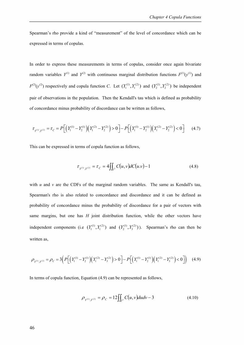
Chapter 4 Copula Functions
Spearman’s rho provide a kind of “measurement” of the level of concordance which can be
expressed in terms of copulas.
In order to express these measurements in terms of copulas, consider once again bivariate
random variables Y(1) and Y(2) with continuous marginal distribution functions F(1)(y(1)) and
F(2)(y(2)) respectively and copula function C. Let and be independent
pair of observations in the population. Then the Kendall's tau which is defined as probability
of concordance minus probability of discordance can be written as follows,
(1) (2)1 1( ,Y Y ) )(1) (2)
2 2( ,Y Y
( )( ) ( )( )(1) (2)(1) (1) (2) (2) (1) (1) (2) (2)
1 2 1 2 1 2 1 2,0 0CY Y
P Y Y Y Y P Y Y Y Y⎡ ⎤ ⎡= = − − > − − −⎣ ⎦ ⎣τ τ ⎤< ⎦ (4.7)
This can be expressed in terms of copula function as follows,
( ) ( ) 1.,42)2()1( ,
−== ∫∫ICYYvudCvuCττ (4.8)
with u and v are the CDFs of the marginal random variables. The same as Kendall's tau,
Spearman's rho is also related to concordance and discordance and it can be defined as
probability of concordance minus the probability of discordance for a pair of vectors with
same margins, but one has H joint distribution function, while the other vectors have
independent components (i.e and ). Spearman’s rho can then be
written as,
(1) (2)1 1( ,Y Y ) )(1) (2)
2 3( ,Y Y
( )( ) ( )( )( )(1) ( 2)(1) (1) (2) (2) (1) (1) (2) (2)
1 2 1 3 1 2 1 3,3 0CY Y
P Y Y Y Y P Y Y Y Y⎡ ⎤ ⎡= = − − > − − − <⎣ ⎦ ⎣ρ ρ 0⎤⎦ (4.9)
In terms of copula function, Equation (4.9) can be represented as follows,
( ) 3,122)2()1( ,
−== ∫∫ICYYdudvvuCρρ (4.10)
46

Chapter 4 Copula Functions
For some copula functions, Equations (4.8) and (4.10) have closed-forms. However, for few
copula functions, Equations (4.8) and (4.10) may not be solved analytically.
When the copula functions and measures of association are known, the copula parameter (for
one-parameter copulas) can be estimated from Equations (4.8) or (4.10). This practice will
give an illustration of the level/ordering of dependence of the random variables. As an
example, consider that the random variables are “found” to be independent with joint
distribution H. This means that the random variables are independent when H is a subset of all
possible joint distributions. This subset can be characterized by copula Π(F(1)(y(1)), F(2)(y(2))) =
F(1)(y(1)).F(2)(y(2)) (i.e. copula function that represents joint distribution of independent random
variables). On the other hand, if a random variable is found to be a monotone function to the
other, then their joint distribution function belongs to another subset of all possible joint
distributions. In this case it belongs to one of the bounds of the copula function.
Recall from sub-chapter 3.2 that marginals do not completely determine their (unique) joint
distribution. Because the true form of dependence of the PCs may not be known for sure, the
bounds for copulas may be needed for sensitivity or risk analysis in estimating possible joint
distribution function. Based on the basic properties of copulas, especially the properties
related to the ordering of copulas, lower and upper bounds of copulas for given marginals can
be constructed. The ordering property of copulas can be described as follows. If we have
copulas C1 and C2 and C1(u,v) ≤ C2(u,v) for all u, v in I, than it can be said that C1 is smaller
than C2 (= C2 is larger than C1). This can be written as C1 C2 or C2 C1. This ordering also
reflects the dependence characteristics of random variables with independent, comonotone and
countermonotone as specific forms of dependence.
p f
The Fréchet-Hoeffding bounds are the universal bounds which envelope all possible copulas
given the marginal distribution functions. This can be written in the following inequality,
47

Chapter 4 Copula Functions
W(F(1)(y(1)), F(2)(y(2))) = max(F(1)(y(1)) + F(2)(y(2)) – 1, 0)
≤ C(F(1)(y(1)), F(2)(y(2))) ≤
min(F(1)(y(1)), F(2)(y(2))) = M(F(1)(y(1)), F(2)(y(2))) (4.11)
Where W and M are the lower and upper distribution bounds of the copula C respectively,
which are also copulas in the case of bivariate problem. These bounds also reflect the two
special cases of dependence, namely countermonotone and comonotone. If the dimension of
the copula is > 2, then W is not a copula function. However, as suggested in Nelsen (1999), W
is still the “best-possible” lower bound for p-dimensional copula even when p > 2. With
additional information, these Fréchet-Hoeffding bounds can be improved (Nelsen et.al.
(2004)). This possible improvement will be discussed in chapter 7.
Until this point, the discussion on the basic properties copulas has been motivated by
reliability analysis problem from non-decreasing multivariate degradation data. In this case,
more interest is given in obtaining the estimate of joint distribution function and its
dependency analysis. However, if the data is non-increasing multivariate degradation data or
predicted multivariate time-to-failure (TTF), survival copulas may be needed to model the
data. This is because the reliability at time t can now be defined as ”the probability that a
component of system will perform a required function for a given period of time when used
under stated operating conditions” (Ebeling (1997)) when the data is the predicted TTF or the
probability that the PCs measurements at time t are above the critical levels (i.e. P[Yt(1) > c(1),
..., Yt(p) > c(p)⏐t]) when the data is non-increasing multivariate degradation data.
In order to discuss survival copulas clearly, assume that there are bivariate random variables
T(1) and T(2) that represents the lifetimes of the system related to the first and second failure
mechanism respectively. Assume further that T(1) and T(2) follow marginal distribution
48

Chapter 4 Copula Functions
functions G(1)(t(1)) and G(1)(t(1)) respectively with joint distribution function H. Then, joint
distribution function of the bivariate TTF can be represented as,
H(t(1),t(2)) = P(T(1) ≤ t(1), T(2) ≤ t(2)) (4.12)
Meanwhile, the joint survival function of the system with bivariate TTF can be written as,
H (t(1),t(2)) = P(T(1) > t(1), T(2) > t(2)) (4.13)
Then if C is the copula of random variables T(1) and T(2), their system reliability at time t (in
this case t(1) = t(2) = t) can be expressed in terms of their marginal reliability (G ) functions as:
R(t) = H (t(1),t(2)) = ( ) ( ) ( ) ( )( ))2()2()1()1()2()2()1()1( 1,11 tGtGCtGtG −−+−+ (4.14a)
or can be re-written as,
R(t) = ( ) ( ) ( )( ))2()2()1()1()2()1( ,, tGtGCttH(
= (4.14b)
With C(
that maps I2 into I can be defined as:
( ) ( )vuCvuvuC −−+−+= 1,11,(
(4.15)
C(
is the survival copula of T(1) and T(2). So the function C(
"couples" the joint reliability
function to its univariate margins in a manner completely analogous to the way in which a
copula connects the joint distribution function to its margins. Georges et.al. (2001) have
shown in their paper that the properties of copulas also valid for survival copulas. This
includes the Fréchet-Hoeffding bounds which in the bivariate survival copulas case can be
rewritten as,
( )vuM ,( ( )vuvu −−+−+= 1,1min1 ( )vu,min= = ( )vuM , (4.16a)
Which is the upper Fréchet-Hoeffding bound. The lower bound can be written as,
49

Chapter 4 Copula Functions
( )vuW ,( ( )0,1max1 vuvu −−+−+= ( )0,1max −+= vu = ( )vuW , (4.16b)
There is another approach to construct joint survival function besides (4.15). As shown by
Georges et.al. (2001) and also used by Shemyakin and Youn (2006), joint survival function
can also be defined directly by a copula function since survival copula is a copula function too.
The second approach to assess system reliability can be written as:
R(t) = ( ) ( ) ( )( ))2()2()1()1()2()1( ,, tGtGCttH = (4.17)
However, note that the results of the two approaches (i.e. (4.15) and (4.17) are different except
for radially symmetric copulas, which has property: CC =(
. Frank copula, which is a member
of Archimedean family, is one of the radially symmetric copulas.
The next question is which copula function is to be used for modelling. There are many
families of copulas with different characteristics. In this thesis, how to choose a copula
function will not be discussed. Instead, the copula function will be assumed known. This
topic needs extensive study. The ones that will be discussed here are copulas from elliptical
distribution family and 1-parameter Archimedean copulas. The use of 1-parameter copulas are
motivated by the fact of the copula dependence’s property (i.e. invariant or change in predicted
ways) which will make the reliability bounds analysis more manageable. In the next sub-
chapter, some popular parametric copula functions will be presented.
4.2. Parametric Copulas
In this thesis the copula functions that will be used in the models that will be proposed in the
next chapters are assumed known. There exist parametric and empirical copulas. In this
discussion, only some popular one-parameter copulas will be presented. They are chosen to
be discussed here because they have nice dependence properties and have been applied and
50
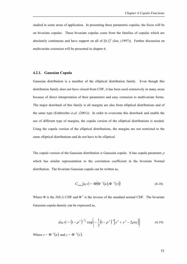
Chapter 4 Copula Functions
studied in some areas of application. In presenting these parametric copulas, the focus will be
on bivariate copulas. These bivariate copulas come from the families of copulas which are
absolutely continuous and have support on all of [0,1]2 (Joe, (1997)). Further discussion on
multivariate extension will be presented in chapter 6.
4.2.1. Gaussian Copula
Gaussian distribution is a member of the elliptical distribution family. Even though this
distribution family does not have closed-from CDF, it has been used extensively in many areas
because of direct interpretation of their parameters and easy extension to multivariate forms.
The major drawback of this family is all margins are also from elliptical distributions and of
the same type (Embrechts et.al. (2001)). In order to overcome this drawback and enable the
use of different type of margins, the copula version of the elliptical distributions is needed.
Using the copula version of the elliptical distributions, the margins are not restricted to the
same elliptical distributions and do not have to be elliptical.
The copula version of the Gaussian distribution is Gaussian copula. It has copula parameter ρ
which has similar representation to the correlation coefficient in the bivariate Normal
distribution. The bivariate Gaussian copula can be written as,
( )vuCGauss , = ( ) ( )( )vu 11 , −− ΦΦΦ (4.18)
Where Φ is the N(0,1) CDF and Φ-1 is the inverse of the standard normal CDF. The bivariate
Gaussian copula density can be expressed as,
= ( vuc , ) ( ) ( ) [ ]⎭⎬⎫
⎩⎨⎧ −+−−−
−− xyyx ρρρ 2121exp1 22122
12 (4.19)
Where x = and y = ( )u1−Φ ( )v1−Φ .
51

Chapter 4 Copula Functions
The copula parameter ρ in (4.18) and (4.18) is simply the usual linear correlation coefficient in
bivariate Normal distribution. When ρ = 0, this copula will result in independence copula.
The comonotonicity is obtained when ρ = 1, while the countermonotonicity is obtained when
ρ = -1. Through the copula parameter ρ, Gaussian copula interpolates among these three
dependency structure (Schmidt (2007)).
This copula has an advantage compared to its bivariate Normal distribution in terms of the
possible use of different marginal distributions. However, it does not have tail dependence
since it is radially symmetric. Therefore, when there is a suspicion that the data may have tail
dependency, this copula may not be the suitable choice for the modelling. In order to define
tail dependence property, consider random variables Y(1) and Y(2) with P[Y(1) ≤ F(1)(y(1)), Y(2) ≤
F(2)(y(2))] = C(u,u). Then a copula is said to have upper (lower) tail dependence if λupper (λlower)
exists in the following equation:
( )u
uuCuuupper −
+−=
→ 1,21lim
1λ (4.20a)
and,
( )u
uuCuupper
,lim0→
=λ (4.20b)
4.2.2. Student-t Copula
Other popular member of elliptical distributions is student-t distribution. It arises in the
context of normally distributed population when the sample size is small. The bivariate
student-t copula is the copula version of bivariate student-t distribution. Similar to Gaussian
copula, this copula also has a linear correlation coefficient ρ and the margins may follow
different distribution functions.
52

Chapter 4 Copula Functions
This bivariate Student-t copula with parameter ρ and υ degree of freedom can be written as,
C(u,v) = Tυ(tυ-1(u), tυ-1(v)) (4.21)
Where Tυ is the bivariate CDF and tυ is the univariate standard student-t distribution with υ
degree of freedom.
= ( vuc , )( ) ( )
21
2
22
2 121
11
+−
⎭⎬⎫
⎩⎨⎧
−−+
+−
υ
ρυρ
ρ
xyyx
(4.22)
where x = and y = . ( )ut 1−υ ( )vt 1−
υ
The difference between this copula and Gaussian copula is that student-t copula has tail
dependence. The upper and lower tail dependence of bivariate Student-t copula are symmetric
and can be written as,
λU = λL = 2tυ+1 ⎟⎟⎠
⎞⎜⎜⎝
⎛
+
−+
ρρ
υ11
1 (4.23)
4.2.3 Archimedean Copulas
Archimedean copulas are considered as an important family of copulas. As indicated by
Embrechts et.al. (2001), this family has been extensively discussed because of some
advantages of this family e.g. they have a great variety of dependence structures and nice
properties. This family is also easy to construct and usually has closed-form expression. The
detail construction of Archimedean copulas will not be discussed here, but some examples of
one-parameter Archimedean copulas will be presented. A brief general definition of
Archimedean copulas will be given first.
53

Chapter 4 Copula Functions
One of the first published literatures that used the term Archimedean copula is by Genest and
Mackay (1986). Most but not all of the copulas in this class extend to the higher dimensions
trough associativity property. In short, bivariate Archimedean copulas can be described as
follows (Nelsen (1999)).
Definition: Let ϕ be a continuous, strictly decreasing function from [0,1] to [0,∞] such that
ϕ(1) = 0. The quasi-inverse of ϕ is the function ϕ[-1] : [0,∞] → [0,1] given by
( ) ( ) ( )( )⎩
⎨⎧
∞≤≤≤≤
=−
−
ttt
t0,0
00,1]1[
ϕϕϕ
ϕ
Note that ϕ[-1] is continuous and decreasing on [0,∞], and strictly decreasing on [0, ϕ(0)].
Furthermore, ϕ[-1](ϕ(u)) = u on [0,1], and
( )( ) ( )( ) ( )⎩
⎨⎧
∞≤≤≤≤
=−
ttt
t0,0
00,]1[
ϕϕϕ
ϕϕ
Finally, if ϕ(0) = ∞, then ϕ[-1] = ϕ-1.
Theorem: Let ϕ be a continuous strictly decreasing function from [0,1] to [0,∞] such that ϕ(1)
= 0, and let ϕ [-1] be the quasi-inverse of ϕ. If C is the function from [0,1]2 to [0,1] given by
C(u,v) = ϕ [-1] (ϕ(u) + ϕ(v)) (4.24)
then C is an copula if and only if ϕ is convex.
In the above definition and theorem, the function ϕ is the generator of the copula. The quasi-
inverse, whose domain is in [0,∞], is an extended inverse function. Compared quasi-inverse
with inverse function of a distribution function, whose domain is in [0,ϕ(0)]. Note Nelsen
(1999) use the terms quasi-inverse and pseudo-inverse to refer to the same things ad defined in
the above definition and theorem. Note also that the terms pseudo-inverse has been reserved
for a matrix inverse-like object that may be defined for a complex matrix, even if it is not
necessarily square. Therefore, in this thesis, quasi-inverse is used to define the above theorem.
54

Chapter 4 Copula Functions
The copula function that is generated as in Equation (4.24) is called Archimedean copula. If
Y(1) and Y(2) are bivariate random variables with continuous marginal distribution functions
F(1)(y(1)) and F(2)(y(2)) and joint distribution H, then based on Archimedean copulas H can be
written as,
ϕ(H(y(1),y(2))) = ϕ(F(1)(y(1))) + ϕ(F(2)(y(2)))
(4.25)
Some one-parameter Archimedean copulas will be presented in this sub-chapter.
Bivariate Frank Copula
Frank copula is an Archimedean copula which has generator function ϕθ(t) = -ln((e-θt-1)/(e-θ-
1)).with θ ∈ (-∞,∞). Based on Equation (4.24), the bivariate Frank copula can be written as,
( )u,vC = ( )( )( )
1 11 ln 11
u ve e
e
θ θ
θθ
− −
−
⎛ ⎞− −⎜− +⎜ ⎟−⎝ ⎠
⎟
)
(4.26)
This copula is the only Archimedean copula that satisfy radial symmetry (C(u,v) = (u,v)). A
copula C is considered as radial symmetry if it satisfies the following equation,
C
= u + v -1 + C(1-u,1-v) for all (u,v) in I2 (4.27) (u,vC
Frank copula is one of the most comprehensive family since it includes countermonocity,
independent and comonocity. As mentioned, this copula is symmetric and additionally it does
not have tail dependence.
Bivariate Clayton Copula
The generator of this copula function is ϕθ (t) = (t-θ - 1)/θ with θ ∈[-1,∞]\{0}. This will give
us Clayton copula as follows,
55

Chapter 4 Copula Functions
) = ( ) ⎟⎠⎞⎜
⎝⎛ −+
−−− 0,1max1θθθ vu (4.28) (u,vC
When the copula parameter θ > 0, the copula is strict and can be written as,
= (u,vC ) ( ) θθθ 11 −
−+ vu (4.29)
For θ > 0, this copula function has lower tail dependence λL = θ1
2−
. Extension to the
multivariate copula is done for the strict Clayton copula.
Bivariate Gumbel-Hougaard Copula
This copula has generator function ϕθ (t) = (-ln t)θ for θ ≥ 1. In some literatures, it is only
called as Gumbel copula. This copula was first discussed by Gumbel. However, since there is
other Archimedean copula with Gumbel’s name and the copula discussed here has been
appeared In Hougaard’s report, it is also called Gumbel-Hougaard copula. This copula can be
written as,
= (u,vC ) ( ) ( )( ) ⎟⎠⎞
⎜⎝⎛ −+−− θθθ 1
lnlnexp vu (4.30)
Gumbel-Hougaard copula does not have lower tail dependence but instead it has upper tail
dependence. The upper tail dependence is λU = θ1
22−
− .
56

Chapter Five
Bivariate Constant-Stress Degradation Test
Consider a system with two failure mechanisms. Both failure mechanisms can be categorized
as degradation failures. The degradation level of the system at certain observation time is
indicated by the levels of the performance characteristics (PCs) of the system observed at that
particular observation time. The degradation failure mechanisms of the system may be
independent or dependent. Common monotonicity of the degradation observations seems a
likely form of dependence because there is likely to be a common usage history if the PCs
reflect system use. Therefore, inclusion of dependence assumption in the model may be
needed in analyzing the bivariate degraded system.
Since the system has two degradation failure mechanisms, a degradation test can be performed
to gather the data needed to evaluate the system. It is assumed that constant-stress degradation
test (CSDT) is sufficient to gather necessary data to evaluate the system. During the test, the
two PCs are observed and measured at predetermined observation times. The measurements
of the both PCs are random variables Yt = {Yt(1), Yt
(2)} at observation time t. Assume that the
57
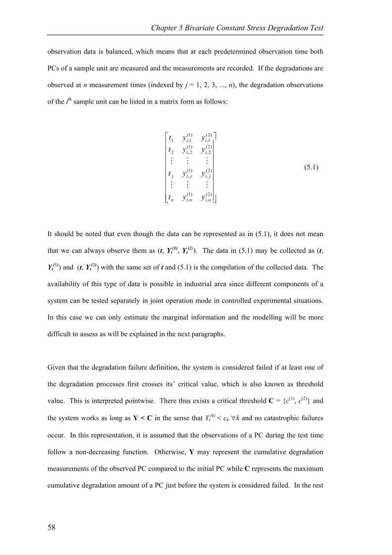
Chapter 5 Bivariate Constant Stress Degradation Test
observation data is balanced, which means that at each predetermined observation time both
PCs of a sample unit are measured and the measurements are recorded. If the degradations are
observed at n measurement times (indexed by j = 1, 2, 3, ..., n), the degradation observations
of the ith sample unit can be listed in a matrix form as follows:
(5.1)
⎥⎥⎥⎥⎥⎥⎥⎥
⎦
⎤
⎢⎢⎢⎢⎢⎢⎢⎢
⎣
⎡
)2(,
)1(,
)2(,
)1(,
)2(2,
)1(2,2
)2(1,
)1(1,1
ninin
jijij
ii
ii
yyt
yyt
yytyyt
MMM
MMM
It should be noted that even though the data can be represented as in (5.1), it does not mean
that we can always observe them as (t, Yt(1), Yt
(2)). The data in (5.1) may be collected as (t,
Yt(1)) and (t, Yt
(2)) with the same set of t and (5.1) is the compilation of the collected data. The
availability of this type of data is possible in industrial area since different components of a
system can be tested separately in joint operation mode in controlled experimental situations.
In this case we can only estimate the marginal information and the modelling will be more
difficult to assess as will be explained in the next paragraphs.
Given that the degradation failure definition, the system is considered failed if at least one of
the degradation processes first crosses its’ critical value, which is also known as threshold
value. This is interpreted pointwise. There thus exists a critical threshold C = {c(1), c(2)} and
the system works as long as Y < C in the sense that Yt(k) < ck ∀k and no catastrophic failures
occur. In this representation, it is assumed that the observations of a PC during the test time
follow a non-decreasing function. Otherwise, Y may represent the cumulative degradation
measurements of the observed PC compared to the initial PC while C represents the maximum
cumulative degradation amount of a PC just before the system is considered failed. In the rest
58

Chapter 5 Bivariate Constant Stress Degradation Test
of this thesis, it will always be assumed that Y is a non-decreasing function of time excepts if
it is defined otherwise. This is illustrated in Figure 5.1 for univariate failure mechanism.
Figure 5.1. Marginal performance characteristic’s degradation path and the threshold value
Based on these, the reliability of the system can be defined as the probability that the system is
working at time t or as the probability that no PCs have crossed the critical level at time t. If
the failure time of the kth PC (i.e. the time that the kth PC first crosses its threshold value) is
random variable T(k), the reliability of a bivariate degradation system can be written as:
R(t) = Ρ[T(1) > t, T(2) > t] = P[Yt(1) < c(1), Yt
(2) < c(2)] (5.2)
If the degradation failure mechanisms are assumed to be independent, the system reliability in
(5.2) can be calculated using the following equation:
R(t) = R(1)(t) × R(2)(t) = P[Yt(1) < c(1)] × P[Yt
(2) < c(2)] (5.3)
The right part of (5.3) is product of the marginal cumulative distribution function (CDF) of the
observations of the PCs at time t. Thus, the marginal CDF of a PC (which is a non-decreasing
function of time) can be represented as:
F(k) (c(k)|t) = P[ Yt (k) < c(k)] (5.4)
t
C(i)
Product’s marginal PDF
PC’s marginal PDF
Y(i)
PC(k) marginal degradation path
59
Chapter 5 Bivariate Constant Stress Degradation Test
On the other hand, if the failure mechanisms are not independent, Equation (5.3) will not give
accurate estimation of the system reliability. In this case, joint CDF of the bivariate
degradation data is needed. As discussed in previous chapters, it is not easy to establish the
joint distribution of a problem when only information of the marginal distributions is
available. Therefore, since we may only have the marginal data because of the experimental
setting, a tool to handle this modelling problem is needed. This is where copula functions
come to our rescue. These functions will also help us to describe the association between the
failure mechanisms, which is possibly not linear.
Our objective is to model the system’s failure mechanisms and predict its reliability using the
data collected from bivariate CSDT. It may not be possible to solve all of its modelling
problems. However, simple alternative models with more flexibility are always welcomed.
The alternative models will be used to model bivariate CSDT data collected in the format (t,
Yt(1)) and (t, Yt
(2)) and with the following possible conditions:
1. The bivariate CSDT is conducted in controlled experimental conditions and the failure
mechanisms may be observed separately in joint operation mode. Therefore, it is more
difficult to estimate and reconstruct the joint distribution of the PCs than if the data is
acquired in the complete form (t, Yt(1), Yt
(2)) simultaneously,
2. Dependency or association between failure mechanisms is indicated by the presence of
common shared factors and it may not be linear. Its existence may affect system
reliability. Therefore, it needs to be taken into account in the modelling and analysis.
An alternative model is needed because the models published in the multivariate degradation
area (i.e. Crk (2000), Huang and Askin (2003), Zhao and Elsayed (2004), Wang and Coit
(2004), Bagdonavicius et.al. (2004), and Xu and Zhao (2005)) either assume independence of
the PCs, multivariate Normal distribution for the joint distribution (which cannot always be
applied in reality), same marginal distribution functions or use modelling with covariates.
60

Chapter 5 Bivariate Constant Stress Degradation Test
For this purpose, three alternative models are presented in this chapter. These models are
proposed to model bivariate CSDT data and overcome the mentioned problems and to be used
to analyze the data and conclude the reliability of a bivariate degraded system. The proposed
models and their assumptions will be presented each in a sub-chapter. Numerical examples of
the models will be presented at the end of the chapter. The data from Bogdanoff and Kozin
(1985) will be used in the example and will be treated as if it is the data of two PCs of a
system. Unfortunately, the results cannot be compared to published models that have used this
data because it has not been used in the context of bivariate degradation system. Nevertheless,
they will give an overview of the proposed models and the bivariate degraded system problem.
This data is chosen because it has published detail degradation readings and can be modified
to serve as an example needed to demonstrate the implementation of the proposed models.
5.1. Bivariate CSDT Model 1
In this sub-chapter, a two-stage model will be proposed. It is mentioned in the beginning of
this chapter that the bivariate degradation data is balanced. However, in this first model, this
assumption is relaxed by allowing the two PCs measured at different predetermined
measurement times. The number of the measurement times of the PCs or the duration of the
observation can also be different. However, the measurement times of a PC should be the
same for all sample units.
Besides addressing the two problems described in the beginning of this chapter, bivariate
CSDT Model 1 will also provide more flexibility by allowing the use of different marginal
degradation and time-to-failure (TTF) distribution families. This is made possible by the use
of copula functions, which will be explained later.
In Model 1, the marginal degradation data will be used to predict the marginal TTF of the PC
in the first stage. This TTF prediction is then used to evaluate both the marginal and system
61

Chapter 5 Bivariate Constant Stress Degradation Test
reliability in the second stage. The basic idea of the first stage of this model is motivated by
the work of Chen and Zheng (2005), in which they present an alternative approach to estimate
the TTF distribution of a system with univariate degradation failure mechanism based on the
individual samples’ TTF prediction using imputation algorithm. However, it focuses only on
single PC and does not take into account the serial-correlation (i.e. correlation between
measurements taken at different points of time) of the PC. With these as motivation, Model 1
is proposed. Before discussing the model, the assumptions related to the test arrangements
and the degradation model, and additional observations/comments will be presented.
It is assumed that the test arrangements fulfilled the followings:
1. The sample units are independent. This means that each sample experiences a bi-/multi-
variate degradation process and the degradation processes between samples are
independent,
2. No catastrophic failures occur,
3. All degradation observations of a PC are made at the same predetermined times.
The second assumption of test arrangements states that no catastrophic failures occur. This is
clearly unrealistic with field data. However, the focus of this thesis is degradation failure
mechanisms modelling. Therefore, the second test arrangement assumption is needed to give
boundary of the problem. This shows the important of controlled experiments in order to get
the needed data to which the proposed models can be implemented.
While the assumptions of the bivariate CSDT Model 1 can be written as follows,
1. The degradation processes are monotone (i.e. non-decreasing process),
2. The distribution of the marginal degradation observations of a PC may be different from
those of other PC, but are assumed to be parametric distributions from exponential family
class or in quasilikelihood forms (i.e. the variance can be an arbitrary function of the
mean),
62

Chapter 5 Bivariate Constant Stress Degradation Test
3. The distribution functions of the marginal time-to-failures (TTFs) may be different but are
assumed to be parametric distributions,
4. Dependence between failure mechanisms is modelled using parametric copulas,
5. The marginal degradation processes are modelled using generalized linear mixed-effect
model (GLMM) which also known as subject-specific (SS) approach.
Some additional observations/comments on the assumptions of the bivariate CSDT Model 1
can be presented as follows,
1. As a consequence of the non-decreasing degradation process assumption, the degradation
process which is not non-decreasing monotone may be transformed, for example by
accumulation of the degradation,
2. Possible within and between samples variation can be captured by the covariance matrix
that is used in the GLMM.
Based on these assumptions, the model is constructed in two stages. The first stage is the
prediction of the individual TTF of the sample units related to each PC. This result can be
used directly to estimate the marginal reliability of the system related to each PC. In the
second stage, information from stage one is used to model the dependency between TTFs
given the critical values and estimate the system joint TTF distribution and reliability. The
first stage will be discussed first in the next sub-chapter.
5.1.1. Model 1 – Stage 1: Marginal TTF Distribution Estimation
For each PC, the marginal degradation data (Y) will be modelled as deterministic function of
time using GLMM. GLMM is a variant of the linear mixed-effect model (see McCullagh and
Nelder (1989) for detail explanation). The linear mixed-effect model is one of most studied
degradation path model popularized by Lu and Meeker (1993). In general, the mixed-effect or
also known as SS model consists of fixed-effects which describe the population (process)
63

Chapter 5 Bivariate Constant Stress Degradation Test
characteristics and random-effects (or mixed-effects) which describe individual unit’s
uniqueness. Using SS model, the average values of the samples’ regression parameters can be
obtained, while the sources of the variability of the regression parameters can be modelled
separately by introducing the random-effect component.
Both linear and non-linear mixed-effect or SS model have been used by many researchers (Wu
and Shao (1999), Bae and Kvam (2004), and Chen and Zheng (2005), etc.) to model univariate
degradation data. The GLMM is a special class of the linear mixed-effect model, where the
response cannot be modelled directly by a linear function but the function of the response can
be modelled by a linear function.
The measurements of kth PC (k = 1, 2) for all m sample units taken at n measurement times can
be listed in a matrix form as follow:
Y(2n × m) = = (5.5) ⎥⎦
⎤⎢⎣
⎡)2(
)1(
YY
⎥⎥⎥⎥⎥⎥⎥⎥
⎦
⎤
⎢⎢⎢⎢⎢⎢⎢⎢
⎣
⎡
)2()2(1
)2(1
)2(11
)1()1(1
)1(1
)1(11
mnn
m
mnn
m
yy
yyyy
yy
K
MM
K
K
MM
K
Then, the general form of the GLMM for both PCs can be written as:
1f − (Yi)= Xi.β + Zi.bi + ei
E(Yi) = f(Xi.β)
Var(Yi) = Vi = R1i + R2i (5.6)
The inverse function of the PC's measurements ( 1f − (Yi)) consists of the value of fixed-effect
part of the degradation process (which is the expected value of the process), a mixed-effect
part which is unique for a sample unit, and an error term (ei).
64

Chapter 5 Bivariate Constant Stress Degradation Test
The fixed-effect part is composed by design matrix (Xi) and common coefficient (β). The
combined design matrix for the ith sample can be written as:
Xi(2n × q)= (5.7) ⎥⎦
⎤⎢⎣
⎡)2(
)1(
00
i
i
xx
Where the sub-matrix (for k = 1,2) can be defined as:
= (5.8) )(kix
⎥⎥⎥
⎦
⎤
⎢⎢⎢
⎣
⎡
)()(1
)(1
)(11
kinq
kin
kqi
ki
k
k
xx
xx
K
MM
K
Where q = (q1 + q2) is the total number of the common degradation parameters for both PCs.
The common coefficient parameter (β) is valid for all samples and can be written as:
= (5.9) ⎥⎦
⎤⎢⎣
⎡= )2(
)1(
ββ
β
⎥⎥⎥⎥⎥⎥⎥⎥
⎦
⎤
⎢⎢⎢⎢⎢⎢⎢⎢
⎣
⎡
)2(
)2(1
)1(
)1(1
2
1
q
q
β
ββ
β
M
M
The second part of the linear function is the mixed-effect part of the sample. Here, Zi is the
design matrix of the mixed-effect part which may have the same or different structure than Xi.
Meanwhile, bi is the mixed-effect regression parameter for the ith sample unit. The structure of
these components depends on the possible characteristics of the process's random-effects. The
components bi and ei are usually assumed to have a standard Normal distribution. However,
this assumption is relaxed in this model. This means of bi and ei can take other values than
zero and their variances may be functions of their means when necessary.
65

Chapter 5 Bivariate Constant Stress Degradation Test
The next element of (5.6) is the variance of Yi which consists of two parts: R1i and R2i. R1i(2n ×
2n) is the within-unit variance-covariance matrix of ith sample unit and R2i(2n × 2n) is the among-
unit variance-covariance matrix of ith sample unit. These can be calculated using the following
equation:
R1i = T1. Γ1 . T1
Di = T2 . Γ2 . T2
R2i = Zi . Di . Zi’
(5.10)
Where,
T = the so-called standard deviation matrix of the within-unit variance-covariance with the
diagonal components T(k)1ij = g(β, bij, Xi, Zi, γ) - the so-called standard deviation function
of the within-unit variation for the kth PC - ith sample at jth measurement time, or T(k)2ij =
h(β, Xi, θ) - which is the so-called standard deviation function of the among-unit
variation for the kth PC - ith sample at jth measurement time,
Γ = the related correlation matrix.
The combined correlation matrix (Γ1) of the within-unit covariance of the bivariate data has a
dimension of (2n × 2n) with the upper-left corner sub-matrix of (n × n) is the correlation
matrix of the first PC, the lower-right corner sub-matrix of (n × n) is the correlation of the
observations of the second PC in a sample taken at all measurement times, while the upper-
right and lower-left corners represent the correlation between the PCs readings of a sample at
particular measurement times (i.e. cross-correlation matrix). The diagonal of the upper-right
corner sub-matrix gives the correlation between two PCs at the same measurement times while
the off-diagonal of this sub-matrix gives the correlation between two PCs measured at
different measurement times. The lower-left corner is the transpose of the upper-right corner
sub-matrix. In the case of different pre-determined measurement times of the PCs, this cross-
correlation matrix can be ignored and each PC is modelled and analyzed separately as
66

Chapter 5 Bivariate Constant Stress Degradation Test
univariate data. The dependency between PCs will then be modelled and analyzed in the
second stage.
The structure of matrix Γ1 is assumed in the beginning since we may not have enough and
accurate information to construct the real correlation matrix. We hope that the correlation
matrix will capture at least the minimal information of the correlation which will be better than
ignoring the possibility of the existence of the correlation. There are some possibilities for the
structure of the correlation matrix, such as: one-dependent correlation or exchangeable
correlation, etc. Another example is based on Markov correlation of a sample where the
degree of correlation depends on the distance of the readings, which can be illustrated as:
Γ1 =
⎥⎥⎥⎥⎥⎥⎥⎥
⎦
⎤
⎢⎢⎢⎢⎢⎢⎢⎢
⎣
⎡
−+−
−+−
+−−
+−−
10
1001
01
''
''
''
''
221
21
221
21
11211
11211
KK
MOMMOM
KK
KK
MOMMOM
KK
jkjkjkjk
jkjkjkjk
jkjkjkjk
jkjkjkjk
tttt
tttt
tttt
tttt
ρρ
ρρρρ
ρρ
(5.11)
The dimension of the correlation matrix of the mixed-effect part (Γ2) depends on the structure
of the mixed-effect part. However, the covariance matrix R2i has the same dimension as R1i
because of the multiplication with Zi.
The last part of variance of the function is the measurement error. Measurement error can also
be included in (5.10) when necessary. It may be presented in the form σ2.Ini which forms a
diagonal variance matrix.
Using (5.6) and its components described in (5.7) – (5.10), the regression parameters that
govern individual samples can be estimated. These are used to predict the TTF of each
sample. The TTF prediction procedure is motivated by Expectation-Maximization (EM) and
67

Chapter 5 Bivariate Constant Stress Degradation Test
single imputation algorithms. These algorithms are known as iterative procedures which deal
with missing data. Some of the earliest publications of the EM idea can be found in Hartley
(1958) and Dempster et.al. (1977) for maximum likelihood estimation (MLE) of incomplete
data. The generalization of method to deal with missing data by filling the missing data with
estimated data is called imputation (Rubin (1976), Little and Rubin (1987) and Schaffer
(1997)) with EM algorithm as one of the approaches. Chen and Zheng (2005) used similar
idea to estimate the TTF distribution function of a univariate degradation data. Motivated by
these ideas, the following TTF procedure is proposed,
1. Make an initial estimation of the regression parameters β, for example using ordinary least
squares (OLS) method without considering the existence of the weights,
2. Using the first estimate of β: β (0) estimate the unknown parameters involved in the
variance functions and in the correlation matrices,
3. Use the estimated variance-covariance and the correlation parameters found in step 2 to
estimate the new regression parameters β (w+1). Then continue to step 2 again. Repeat
step 1 and 2 until convergence is reached,
4. Based on the result of step 3, calculate the value of the PC's measurement at additional
measurement times between the first and last measurement times when possible (i.e. do
interpolation prediction),
5. Re-estimate the regression parameters (step 1 – 3), but now include the estimation in step
4 as additional data point(s). Repeat step 4 and 1 – 3 until the regression parameters and
variance converge,
6. Use the last estimation of regression parameters to predict the TTF of each sample,
7. Find the most probable marginal lifetime distributions based on the TTF prediction and
estimate their distribution parameters.
This procedure is also motivated by the idea that interpolation will give us better estimation
than extrapolation. In interpolation, the prediction is done on unknown data that lies within
68

Chapter 5 Bivariate Constant Stress Degradation Test
the range of available observations while in extrapolation the data predicted is outside the
range. As mentioned by Chao (1999), the further the extrapolation, the bigger the error
(inaccuracy) should be expected. He also suggests that even though the model may be wrong
the extrapolation may still be valid if it is not too far from the observation range. Therefore,
when the condition is possible, interpolation data is included in the above procedure.
In the procedure, initial estimation of β is found using OLS since linear functions are used. It
can be written as:
)0(β)
= ( )1
1
1 1
m mT Ti i i i
i if
−−
= =
⎛ ⎞⎜ ⎟⎝ ⎠∑ ∑X .X X . Y (5.12)
In Equation (5.12) 1f − (Yi) is used instead of Yi because as stated in (5.6) the linear estimation
is applied to the function of the PCs and not directly to the PCs' observation. Only if the link
function is an identity link function where 1f − (Yi) = Yi, then Yi can be used directly in (5.12).
The initial estimate of β is used to estimate the rest of the unknown parameters. These, will
further be used to obtain the new estimates of β. This is done iteratively using weighted least
squares equation, to take into account the differing precision of each response, which can be
written as:
( )1
1 1
1 1
m mT Ti i i i i i
i if− −
= =
⎛ ⎞= ⎜ ⎟⎝ ⎠∑ ∑
) ) )β
_1−X .V . X X .V . Y
(5.13)
After the unknown parameters are converged, then bi can be calculated from the following
equation:
( )( )1 1T
i i if− −= − βi iˆ ˆˆ ˆb D.Z .V Y X . (5.14)
69
Chapter 5 Bivariate Constant Stress Degradation Test
And the results can be used to predict the TTF of each sample, which is the time that the PC of
a sample first reaches its threshold value. These TTF predictions can be utilized to estimate
the marginal failure time distribution using the usual probability methods such as probability
plot and likelihood-ratio method. In this thesis, Akaike Information Criterion (AIC) will be
used to choose distribution function. AIC will be explained in the later part of this thesis.
Then, the kth marginal reliability can be estimated as R(k)(t) = Ρ[T(k) > t].
The next step is to combine and use the results to estimate the system reliability, which is our
main purpose. This will be discussed in the next sub-chapter.
5.1.2. Model 1 – Stage 2: System Reliability
The bivariate CSDT data may be observed in the forms of (t, Yt(1)) and (t, Yt
(2)). Therefore,
additional information is needed to model and analyze the data as a bivariate system, while the
marginal conclusion can be obtained easier. Knowing the marginal distributions only will not
lead to a unique joint distribution. Furthermore, if the marginal distributions follow different
distribution families, the difficulty of joint distribution construction increases significantly.
This is where copula functions come to our rescue.
It has been discussed in Chapter 4 that copula functions can be used to model multivariate
dependency (even when the dependency is non-linear) separately from the marginal data
modelling. Therefore, copulas can be used to model dependency between the two failure
mechanisms in bivariate CSDT problem and to estimate the TTF joint distribution which is
needed to evaluate system reliability. In applying copula to bivariate CSDT problem, there are
some issues that need to be taken care of. For examples: which copula function to be
implemented to the problem, tail dependency issues, adjustment of the result to reflect joint
PDF of the system during the life of the system, and upper and lower bounds of the joint
70

Chapter 5 Bivariate Constant Stress Degradation Test
distribution and system’s reliability. In this chapter we will focus on the implementation of
these copulas in bivariate CSDT modelling and the copula function is assumed to be known.
Its utilization in Model 1 will be discussed as follows.
In the stage 1 of Model 1, the predicted TTF data of both PCs is obtained for all samples.
Based on this result, the marginal TTF distribution functions are evaluated and the marginal
distribution parameters are estimated. Let T(1) the random variable of TTF of the first PC and
T(2) the random variable of TTF of the second PC. Further, let G(1) the CDF of the failure time
of the first failure mechanism and G(2) the CDF of the failure time of the second failure
mechanism. Then, the joint distribution function of the bivariate TTF data can be represented
using copula (C) as:
H(t(1),t(2)) = C(G(1)(t(1)), G(2)(t(2)))
(5.15)
It is obvious from (5.15) and the discussion in chapter 4, that the joint survival function can be
estimated when the copula function is known. Recall, that if C is the copula of random
variables T(1) and T(2), their system reliability at time t (in this case t(1) = t(2) = t) can be
expressed in terms of their marginal reliability (G ) functions as:
R(t) = H (t(1),t(2)) = ( ) ( ) ( ) ( )( ))2()2()1()1()2()2()1()1( 1,11 tGtGCtGtG −−+−+ (5.16a)
or can be re-written as,
R(t) = ( ) ( ) ( )( ))2()2()1()1()2()1( ,, tGtGCttH(
= (5.16b)
Where C(
is the survival copula of T(1) and T(2). The function C(
"couples" the joint reliability
function to its univariate/marginal reliability functions in a manner completely analogous to
the way in which a copula connects the joint distribution function to its margins. For analysis
71

Chapter 5 Bivariate Constant Stress Degradation Test
of Model 1 – stage 2, t(1) = t(2) = t because what we want to evaluate is the system reliability at
certain observation time t, which is the same time point for both PCs.
There is another approach to construct joint survival function besides (5.16). As shown by
Georges et.al. (2001) and also used by Shemyakin and Youn (2006), joint survival function
can also be defined directly by a copula function since survival copula is a copula function too.
It can be written as:
R(t) = ( ) ( ) ( )( ))2()2()1()1()2()1( ,, tGtGCttH = (5.17)
Note that the two approaches (i.e. (5.16) and (5.17)) give different results except for radially
symmetric copulas.
The copula parameter can be estimated based on the predicted TTFs and the copula function.
Assume that the copula function used is 1-parameter copula. There are three possible ways to
obtain the copula parameter. For the first way, predicted TTF data is used. Recall that
Kendall's tau is related to copula function (C) through the following equation:
( ) ( ) 1,,42
−= ∫∫IC vudCvuCτ (5.18)
Therefore, if the measure of association Kendall's tau of the TTF data of the two failure
mechanisms can be calculated, then the copula parameter can be estimated from (5.18).
Unfortunately, the closed-form function or analytical solution of (5.18) can be obtained but not
for every copula. When the analytical solution of (5.18) cannot be obtained, a numerical
analysis method can be performed to estimate the copula parameter.
To use (5.18), the Kendall's tau value of the TTF data has to be calculated. If ( ))2(1
)1(1 ,TT and
( ))2(2
)1(2 ,TT are pairs of the TTF random variables which are independent and identically
72

Chapter 5 Bivariate Constant Stress Degradation Test
distributed, each with joint distribution function H, then these can be used to calculate
Kendall’s tau. In order to calculate Kendall's tau from the predicted TTF data of both PCs, the
following equation can be used,
( )( )[ ] ( )( )[ ]00 )2(2
)2(1
)1(2
)1(1
)2(2
)2(1
)1(2
)1(12,1 <−−−>−−= TTTTPTTTTPτ (5.19)
Equation (5.19) describes Kendall’s tau calculation of the two TTF random variables. It can
be explained as the difference between probability of concordance and the probability of
discordance. Substituting (5.19) into (5.18) will lead us to obtain the copula parameter, which
is the last ingredient of our calculation.
The second possible way to obtain copula parameter is through inference function of marginal
(IFM) method. IFM strategy relies heavily on MLE method and therefore it can be expected
that the results will be quite effective. In IFM, the marginal distribution parameters are
estimated first. These estimated marginal parameters are then used to estimate the “copula”
part of the likelihood function. Since the samples are assumed independent and the marginal
distribution functions can be estimated separately, the full log-likelihood function of a
bivariate copula of the TTF data can be written as,
(5.20) ( ) ( ) ( ) ( )( ) ( ) ( )∑∑==
+=m
i
ki
km
iii TgTGTGcL
1
)(
1
)2(2)1(1 ln,ln
In (5.20), c is the copula density function which is derived from C, while g is the marginal
density functions of the marginal TTF data. Since the marginal distribution parameters have
been estimated in stage 1 of Model 1, then corporation of IFM is suitable to obtain the copula
parameter. These estimated marginal distribution parameters are used to estimate the copula
parameter by maximizing the “copula” part of (5.20) which is:
( ) ( ) ( ) ( )( )∑=
m
iii TGTGc
1
)2(2)1(1 ˆ,ˆln (5.21)
73

Chapter 5 Bivariate Constant Stress Degradation Test
As investigated by Xu (1996), this IFM method is effective (i.e. the ratio of the mean square
errors of IFM estimators and MLE estimators is closed to 1). There are other studies of the
effectiveness of this two-stage likelihood estimation (i.e. Joe (2005) and Andersen (2005)),
which also shows that IFM is quite effective for our purpose. The result of maximizing (5.21)
with respect to the copula parameter, will give the estimation of the copula parameter. This
can be used in (5.16) or (5.17) to assess the system reliability from the TTF marginal data.
If the measurement times of both PCs are the same, the cross-correlation matrix as a diagonal
matrix and the correlation between PCs is not a function of time and therefore has the
correlation value (ρ3) for all measurement times, then its relationships with non-parametric
correlation parameter's Kendall's tau ( 2,1τ ) can be expressed by (Kruskal, 1958):
⎟⎟⎠
⎞⎜⎜⎝
⎛=
2sin 2,1
3
πτρ (5.22)
The estimated Kendall's tau ( 2,1τ ) can be used to estimate the dependency between the
degradation failure processes. However, it must be noted that the copula parameter obtained
from this third approach does not describe the dependency between the TTFs. Therefore, it is
not advisable to convert (5.22) results into copula parameter using (5.18) since it will describe
the wrong dependence characteristic.
The system reliability can now be evaluated using (5.16) or (5.17) based on the predicted TTF
data of both failure mechanisms and estimated copula parameter with assumption that the
copula function is known.
74

Chapter 5 Bivariate Constant Stress Degradation Test
5.2. Bivariate CSDT Model 2
In this second proposed model, the marginal and system reliability are assessed from the
estimated marginal degradation CDF parameters instead. The idea used in Model 2 is to
obtain the marginal CDF parameters at all measurement times and predict their values at other
concerned times. Therefore, stage 1 of Model 2 consists of estimating the distributions of the
marginal degradation data and their parameters at all measurement times and performing a
regression on those parameters to enable us to predict the parameters values at other times.
This strategy has been suggested by Huang and Askin (2003) to estimate the marginal
reliability of system with degradation characteristics, but with independent PCs assumption.
However, they do not discuss how to use the strategy when exists possible serial dependency
of the observations. These problems will be handled in Model 2.
Because of the strategy adopted by Model 2, the measurement times of the samples should be
the same for all PCs or in other word, the data should be balanced. This is because PC
observations data taken at the same measurement time is needed to estimate the marginal
distribution parameters at certain measurement time and to assess the dependency/correlation
between PCs. Even though Model 2 is more restricted than Model 1 in term of the flexibility
of determining the measurement times, it is more flexible than Model 1 in term of the possible
choices of the marginal degradation CDF.
Since regression will be done on the marginal CDF parameters, than more distribution
functions can be considered to represent the marginal data because there is less restrictions on
the choices of the distribution function. Nevertheless, it should be remembered that only one
distribution function can be used to model a PC because regression is performed on
degradation distribution parameter(s).
The first and second assumptions of the test arrangement of Model 2 are the same with those
of Model 1. However, the third test arrangement assumption of Model 2 requires all
75
Chapter 5 Bivariate Constant Stress Degradation Test
degradation observations of both PC to be made at the same predetermined times. On the
other hand, only the first and fourth assumptions of the degradation model assumptions of
Model 1 are also used in Model 2. Additional degradation model assumptions of Model 2 are:
1. The marginal degradation distribution function of a PC follows a the same parametric
distribution function at all measurement times and can be different than the marginal
degradation distribution of the other PC,
2. The marginal degradation distribution parameters are assumed independent and may be
functions of time,
3. The marginal degradation distribution parameters are modelled using univariate
generalized linear model (GLM) and assumed to follow Normal distribution function.
The first observation/comment on the assumptions of the bivariate CSDT Model 2 is the same
with the first comment on the assumptions of Model 1 with the second comment can be stated
as: possible variation can be captured by an estimated correlation matrix that is used to
construct the covariance matrix of the GLM.
With these assumptions, the two stages of Model 2 will be discussed. Stage 1 of Model 2
consists of fitting of the marginal probability functions, estimating the marginal distribution
parameters, conducting regression on each marginal distribution parameter and assessing
marginal reliability of each PC. Then, the estimation of the between PCs’ correlation and
analysis of the system reliability are conducted in the second stage. The copula function in
Model 2 is assumed known.
5.2.1. Model 2 – Stage 1: Marginal Degradation Distribution Modelling
Consider the marginal PC observation data that can be listed in a matrix form as follows,
76
Chapter 5 Bivariate Constant Stress Degradation Test
Y(k)(n × m) = (5.23)
⎥⎥⎥
⎦
⎤
⎢⎢⎢
⎣
⎡
)()(1
)(1
)(11
kmn
kn
km
k
yy
yy
K
MM
K
First, evaluate which distribution function that best fits the data in every column of the matrix
of (5.23). AIC is one of the methods that can be used to compare which probability density
function best fits to all columns. Then, the rest of the procedure starts from the chosen
marginal distribution functions. The complete steps of stage 1 can be written as follows:
1. Evaluate the distribution functions that fit best to the marginal degradation data, one
distribution for each PC,
2. For each PC, estimate the distribution parameters at each measurement time based on the
assumed distribution function of each PC as concluded in step-1,
3. Focus on a marginal distribution parameter. If it is considered as a function of time,
model it using GLM with assumption that it is normally distributed with possible serial
dependency between the marginal distribution parameter estimated at different
measurement times,
4. If the marginal distribution parameter is considered not a function of time, find the mean
value and use it as the value of the marginal distribution parameter at all measurement
time,
5. Do step 3 and 4 to all marginal distribution parameter,
6. Use the estimated and predicted marginal distribution parameters to estimate and analyze
marginal reliability functions of both PCs.
Regression is performed on the marginal degradation distribution parameters. As an
illustration, consider for an example that the degradation data of a PC can be represented by
Normal distribution. In this case, estimate normal distribution parameters (μ and σ) from the
PC degradation data at every measurement time. If we assume that the parameter μ is a
function of time while the parameter σ is not a function of time, then regression is performed
77

Chapter 5 Bivariate Constant Stress Degradation Test
on the μ estimation while the mean value of σ is used as estimation. Consequently, no
regression on σ is needed.
For simple illustration, consider a distribution parameter of a marginal degradation data. The
matrix of marginal degradation distribution parameter (U) estimations from data observed at
n-measurement times can be written as:
U(n×1) = (5.24) ⎥⎥⎥
⎦
⎤
⎢⎢⎢
⎣
⎡
nu
uM1
Regression on these data will be done using GLM with Normal distribution assumption. The
data in (5.24) is non-repeatable and therefore no random-effect is present. As a consequence,
the regression model of the marginal distribution parameter can be written as:
E(U) = f(X.β)
Var(U) = V = σ2.Γ = T.Γ.T (5.25)
The function of the marginal distribution parameter is represented by a linear function. If the
distribution parameter data follows linear function then identity link function is used in the
expectation of U. And as a consequence of the Normal distribution assumption of the
variance, the so-called "standard deviation" matrix T is a diagonal matrix with σ as the
diagonal components.
The design matrix (X) in the (5.25) has dimension of (n × q) and can be written as:
X = (5.26) ⎥⎥⎥
⎦
⎤
⎢⎢⎢
⎣
⎡
nqn
q
xx
xx
K
MM
K
1
111
78

Chapter 5 Bivariate Constant Stress Degradation Test
With the index j = 1, ..., n represents the number of measurement times and q is equal to the
number of the regression coefficient parameters. Meanwhile, the regression coefficient
parameter (β) can be written as:
β = (5.27) ⎥⎥⎥
⎦
⎤
⎢⎢⎢
⎣
⎡
qβ
βM1
In order to estimate the unknown parameters in (5.25), iterative re-weighted estimation can be
used. The iterative re-weighted estimation procedure can be re-written as:
1. Make an initial estimation of the regression parameters β for example using ordinary least
squares (OLS) method without considering the existence of the weights,
2. Somehow, use the first estimate of β: β (0) to estimate the unknown parameters of the
correlation matrix and σ,
3. Based on the estimation of variance and the correlation matrix estimated in step 2,
estimate again the new regression parameters β (w+1) using iteratively re-weighted least
squares. Then continue to step 2 again. Repeat steps 2 and 3 until convergence.
The first step of the iterative re-weighted procedure can be executed using equation similar to
(5.12), which can be written as:
)0(β)
= ( ) ( )UXXX 11 −−fTT ... (5.28)
While the weighted least square equation used here is the modification of (5.13) which can be
written as:
( ) ( )UVXXVXβ 1111 −−−= fTT ....._ )))
(5.29)
79

Chapter 5 Bivariate Constant Stress Degradation Test
Notice that compared to (5.12) and (5.13), there is no-Σ operation in (5.28) and (5.29) because
for each measurement time, there is only one marginal degradation distribution parameter data
available. If there are more than one set of bivariate CSDT data, then the-Σ will appear again
in (5.28) and (5.29).
Since there is only one design matrix in (5.28) and (5.29), because there is no repeatable
measurements of the marginal degradation parameter (U), then the estimation of the unknown
parameters in the variance matrix (V) is easier then in Model 1. It is done by finding the
correct combination of the unknown parameters in V in the following function:
{ } 01
2
=−−
VβXU ).(f
(5.30)
The final estimated regression parameters are used to estimate and predict the value of the
marginal degradation distribution parameters, which are used to estimate the marginal
degradation CDF of the PCs using Equation (5.4). The estimated CDF can be treated as
marginal reliability estimation since the PCs are assumed as non-decreasing functions. Using
the result of stage 1 the system reliability can be evaluated in stage 2 of Model 2.
5.2.2. Model 2 – Stage 2: System Reliability
A copula function is also exploited here to analyze the correlation between the marginal failure
mechanisms. However, instead of using it for analyzing correlation between TTF, it is used to
analyze the correlation between the degradation observation data.
To assess and estimate the correlation between PCs using measure of association Kendall’s
tau, the measurement times of both PCs have to be the same. If ( ))2(1
)1(1 ,YY and ( ))2(
2)1(
2 ,YY
are pairs of the degradation observation random variables which are independent and
80

Chapter 5 Bivariate Constant Stress Degradation Test
identically distributed, each with joint distribution function H, then the Kendall’s tau value can
be calculated as the difference between concordance and discordance of the PCs observation
data at certain measurement time, which can be written as,
( ) ( )( )[ ] ( )( )[ ]tYYYYPtYYYYPt 00 22
21
12
11
22
21
12
1121 <−−−>−−= )()()()()()()()(
,τ (5.31)
There will be one value of measure of association between PCs for each measurement time. If
it has no trend, the average can be used to illustrate the correlation between PCs and used
directly to estimate the copula parameter via (5.18). Otherwise, regression should be
performed on this measure of association. The regression result is used to estimate the copula
parameter at certain time. Alternatively, the measure of association is converted into copula
parameter first before the regression analysis is performed.
The second method to estimate the correlation between PCs is using IFM method. The
equations used to do this are (5.20) and (5.21) with some modification of the components used
in the equations. In Model 2, the marginal distribution functions used are not the marginal
TTF distribution (G(k)) but the marginal PCs distribution functions (F(k)). Therefore, Equations
(5.20) and (5.21) are modified into:
( ) ( ) ( ) ( ) ( )( ) ( ) ( )∑∑==
+=m
i
kij
km
iijij tYftYFtYFctL
1
)(
1
)2(2)1(1 ln,ln (5.32)
( )( ) ( )( )( )∑=
m
iijijijij tYFtYFc
1
2)2(1)1( ˆ,ˆln (5.33)
A copula parameter estimation will be obtained for each measurement time. Therefore, if
there is no evidence that the copula parameter of the PCs joint distribution is a function of
time, then the average can be used as the copula parameter value for all measurement times.
Otherwise, regression should be performed. IFM is more straight forward and efficient than
MLE (since it uses less calculation resources) and utilizes all the dependence information.
81
Chapter 5 Bivariate Constant Stress Degradation Test
The estimated copula parameter and of course with the chosen copula function, are then used
to estimate and assess the system reliability in the following equation,
R(t) = P[Yt
(1) < c(1)⏐t, Yt(2) < c(2)⏐t] = C{F(1)(y(1)|t), F(2)(y(2)|t)} (5.34)
Equation (5.34) is valid for non-decreasing bivariate PC observation. It is used to assess the
joint survival function of the system and gives some flexibility incorporating dependency
assumption between PCs and the use of different distribution functions to represent the
marginal PCs.
5.3. Bivariate CSDT Model 3
Bivariate CSDT Model 3 also consists of two stages, where the first stage focuses on the
analysis of the PCs' observations regression components and estimation of the marginal
distribution related parameters. The second stage mainly focuses on the estimation of
correlation between PCs and assessing the joint distribution and system reliability.
Similar to Model 2, flexibility of having different measurement times for observations of
different PCs as in Model 1 cannot be exercised in Model 3. This is because the between PCs'
dependency will be assessed directly from the degradation data, which will be discussed as
follows.
GLM with population-average (PA) approach will be used in Model 3 because individual
estimation is not needed. In addition, the marginal distribution functions of the bivariate
degradation data should be estimated directly or indirectly. Therefore, only distribution
functions whose distribution parameters can be defined from the mean, variance, or their
functions can be used in this model.
82

Chapter 5 Bivariate Constant Stress Degradation Test
The assumptions of the test arrangement of Model 2 are also valid for Model 3. In addition,
the first and fourth model assumptions of Model 1 are also valid for Model 3 with additional
model assumption as follows:
1. The distribution of the marginal degradation observations of a PC may be different from
those of other PC, but are assumed to be parametric distributions whose distribution
parameter(s) may be estimated from a function of the mean and/or variance components of
the degradation regression model. For example, from exponential family class,
2. The marginal degradation observations are modelled using generalized linear model
(GLM) with population-average (PA) approach.
Meanwhile the additional observations/comments of Model 3 are the same with those of
Model 1.
5.3.1. Model 3 – Stage 1: Degradation Data and Marginal Reliability Modelling
Since we can only model the mean and variance of the data in the GLM while we also need to
estimate the marginal CDF of the degradation data, then the possible choices for the marginal
distribution functions is more limited compared to Model 2.
In general, the data for this model can be presented in the form of (5.5), but since random-
effect is not of interest, the model can be written as follows:
1−f (Yi)= Xi.β + ei
E(Yi) = f(Xi.β)
Var(Yi) = Vi = Ti.Γ.Ti (5.35)
The forms of some of the regression components (i.e design matrix X and regression
parameters β) are as in (5.7), (5.8), and (5.9). There are no Zi and bi in Model 3 because PA
approach is used. In GLM-PA approach, the mean function represents the population mean
83

Chapter 5 Bivariate Constant Stress Degradation Test
function. The model has combined variance-covariance matrix with dimension (2n × 2n) since
it is assumed that the number of measurement times for both PCs is the same.
And since there is no random-effect in this model, there is no R2i (= Zi.Di.Zi’) in the model.
The so-called standard deviation matrix Ti in (5.35) consists of the standard deviation
functions of the marginal degradation data as the diagonal elements (each diagonal element
represents each measurement time) and zeros at other elements of the matrix. Depends on the
marginal distribution functions, the standard deviation may be a function of the mean and the
diagonal element of Ti may be written in the following form:
Tij(k) = g(k)(β(k), θ(k), xij
(k)) (5.36)
Where Tij(k) is the standard deviation of kth PC ith sample at jth measurement time. The
unknown parameters of the standard deviation function g(k) of the kth PC is presented as θ(k).
These unknown parameters have to be estimated during the iterative re-weighted procedure to
re-estimate the regression parameters β.
Other component of Vi is Γ. Similar to Γ1 in (5.11), Γ in (5.36) can have four sub-matrices
with the upper-right and lower-left sub-matrices represent the cross-correlation between PCs.
However, its element may take different form than Γ1 depends on the dependence assumption.
Iterative re-weighted method is also used to estimate the unknown parameters. The unknown
parameters (i.e. θ and unknown parameters in matrix Γ) of the covariance matrix Vi can be
estimated using general estimating equation (GEE), that is made popular by Liang and Zeger
(1986). After the unknown parameters in (5.35) have been estimated, the result can be used to
estimate the marginal CDFs of the degradation data which can be interpreted as the marginal
reliability functions of the system since the degradation data is assumed to be non-decreasing
function. This is done by calculating the marginal CDF distribution parameters using the
84

Chapter 5 Bivariate Constant Stress Degradation Test
equation that links these distribution parameters to the mean and variance components of the
GLM. In some cases, for example in Normal distribution, the mean and variance obtained in
the regression analysis (GLM) have identity link to the parameters μ and σ of the Normal
distribution respectively. Therefore, they can be used directly to estimate the marginal CDF
and marginal reliability of the system. Another example of distribution function that can be
used to model continuous marginal degradation data is Gamma distribution, which can be
written as,
( ) ⎟⎟⎠
⎞⎜⎜⎝
⎛−⎟⎟
⎠
⎞⎜⎜⎝
⎛Γ
=μσμσσ
σ
2
1
22 exp11)(
2 yyy
yf (5.37)
Equation (5.37) gives estimation of the probability density value of a marginal degradation
observation, y, when the mean (E(Y(k)) and variance (V(k)) of the marginal degradation data are
interpreted as μ and σ2μ2 of (5.37) respectively. The symbol Γ in (5.37) is not estimated
correlation matrix, but it is a gamma function.
Because the marginal degradation distribution parameters can be estimated through certain
link functions to the (components of) mean and variance of the degradation data, then the
marginal reliability of non-decreasing degradation process can be estimated using (5.4).
If the PCs is modelled simultaneously, then the cross-correlation parameter which represents
the between PCs product-moment correlation will also be obtained. It can be used to find the
copula parameter of the copula function that joint the marginal distribution functions. If, for
example, the cross-correlation matrix is defined as diagonal matrix with all diagonal
component the same (i.e. the cross-correlation parameter (ρ3) is not a function of time), then
the measure of association Kendall’s tau of the PCs (τ1,2 = τC) can directly be obtained using
(5.22). This Kendall’s tau can therefore be translated to the copula parameter using (5.28) if
85

Chapter 5 Bivariate Constant Stress Degradation Test
the copula function is known. However, one may prefer to estimate the copula parameter
using IFM with the reason as mentioned in the previous sub-chapters.
5.3.2. Model 3 – Stage 2: System Reliability
The stage 2 of Model 3 is basically the same with Model 2 except that the copula parameter
can be alternatively estimated from the cross-correlation parameter obtained in the stage 1 of
Model 3. However, since there are two conversions needed to get the copula parameter from
cross-correlation parameter, there is higher possibility of accumulation of estimation error that
can be occurred from the rounding of the previous conversion. Besides, estimating copula
parameter from the cross-correlation parameter will not capture additional dependence
information. Therefore, IFM may be preferred to estimate the copula parameter.
Using IFM, the copula parameter is obtained by maximizing (5.33) with respect to the copula
parameter. The result is used to estimate and assess the system reliability. Equation (5.34)
also expresses the system reliability at time t when the marginal degradation reliability
functions (i.e. F(k)(y(k)|t)) are known.
5.4. Numerical Example
To demonstrate the implementation of the proposed bivariate CSDT models, the models will
be employed on a numerical example. The numerical data is taken from Bogdanoff and Kozin
(1985). This data is chosen since it has detail degradation observations compared to other
published data and the measurements at failure times are also recorded for comparison with
the proposed model. In the original data, 21 samples are tested for fatigue crack development
and the measurements are taken at the same measurement times. The time unit is in million
cycles. Since the focus of the proposed models is to analyze bivariate CSDT data, the data
86

Chapter 5 Bivariate Constant Stress Degradation Test
will be treated as if half of it is the first PC and the other half represents the second PC. As a
consequent of the pairing, only 20 degradation paths will be used.
To fit this data in the context of bivariate degraded system, additional assumption is needed. It
will be assumed that there is a system with two possible fatigue crack positions and this
assumption is valid for every sample. The left-hand crack (position A) of a sample (i.e the
first 10 paths of the data) represents the first PC, while the right-hand crack (position B) of a
sample (i.e. the rest of the paths) represents the second PC. Figure 5.2 gives illustration of the
bivariate problem modified from the data of Bogdanoff and Kozin (1985).
1st crack position A
Figure 5.2. Crack locations of the system/product that represents the two performance
characteristics
2nd crack position BCrack size
The data that will be used is the data measured only until 0.09 million cycles. The sample is
considered failed if the crack found in at least one location exceeds the maximum amount
allowed for that particular location. Examples of reading the crack data at Table 5.1 are
presented as follows,
Sample no. 5 at measurement time 0.01 million cycles (= second measurement time):
1st PC observation = = 0.94 )1(
2,3Y
2nd PC observation = = 0.92 )2(
2,3Y
Sample no. 7 at measurement time 0.04 million cycles (= fifth measurement time):
1st PC observation = = 1.07 )1(
5,7Y
2nd PC observation = = 1 )2(
5,7Y
87

Chapter 5 Bivariate Constant Stress Degradation Test
Table 5.1. Fatigue crack (inch) data adapted from Bogdanoff and Kozin (1985) Samples Million
Cycles PC 1 2 3 4 5 6 7 8 9 10
0 1 0.9 0.9 0.9 0.9 0.9 0.9 0.9 0.9 0.9 0.9 0.01 0.95 0.94 0.94 0.94 0.94 0.94 0.94 0.93 0.92 0.92 0.02 1 0.98 0.98 0.98 0.98 0.98 0.98 0.97 0.97 0.96 0.03 1.05 1.03 1.03 1.03 1.03 1.03 1.02 1 1.01 1 0.04 1.12 1.08 1.08 1.07 1.07 1.07 1.07 1.06 1.05 1.04 0.05 1.19 1.14 1.13 1.12 1.12 1.12 1.11 1.11 1.09 1.08 0.06 1.27 1.21 1.19 1.19 1.19 1.18 1.17 1.17 1.15 1.13 0.07 1.35 1.28 1.26 1.25 1.24 1.23 1.23 1.23 1.21 1.19 0.08 1.48 1.37 1.35 1.34 1.34 1.33 1.32 1.3 1.28 1.26 0.09 1.64 1.47 1.46 1.43 1.43 1.41 1.41 1.39 1.36 1.34
0 2 0.9 0.9 0.9 0.9 0.9 0.9 0.9 0.9 0.9 0.9
0.01 0.9 0.93 0.92 0.93 0.92 0.92 0.93 0.92 0.92 0.92 0.02 0.96 0.97 0.97 0.96 0.96 0.95 0.96 0.94 0.94 0.94 0.03 1 1 0.99 1 0.99 0.97 0.97 0.97 0.97 0.97 0.04 1.04 1.03 1.03 1.03 1.03 1 1 1.01 0.99 0.99 0.05 1.08 1.07 1.06 1.07 1.06 1.03 1.05 1.04 1.02 1.02 0.06 1.13 1.1 1.1 1.12 1.1 1.07 1.08 1.07 1.05 1.05 0.07 1.18 1.16 1.14 1.16 1.16 1.11 1.11 1.09 1.08 1.08 0.08 1.24 1.22 1.2 1.2 1.21 1.16 1.16 1.14 1.12 1.12 0.09 1.31 1.29 1.26 1.26 1.27 1.22 1.2 1.19 1.16 1.16
There are two failure scenarios that will be studied here:
1. The maximum crack amount allowed at both locations A and B is the same, i.e. 1.6 inches
(which is 77.78% accumulative increment from first measurement at 0.9 inch). If at least
one location has a crack that reaches this threshold value, the sample is considered failed.
This definition is also used in Lu and Meeker (1993),
2. Assume that the severity of locations A and B is different and different threshold values
are imposed for each location. In this case, threshold values of the accumulative crack
increment are 80% (PC at 1.62 inch) and 40% (PC at 1.26 inch) for location A (i.e. 1st PC)
and B (i.e. 2nd PC) respectively.
The data in Table 5.1 will be modelled and analyzed using the three proposed models. The
results will be discussed and compared. Some comments on the use of each model will be
given in Sub-chapter 5.5.
88

Chapter 5 Bivariate Constant Stress Degradation Test
5.4.1. Model 1 Example
In the first stage of Model 1, it is assumed that the function of the degradation observation of a
PC can be represented by a linear function in the form of X.β as in Equation (5.6). The model
for this example can be defined as:
1−f (Yi) = Xi.β + Zi.bi + ei
E(Yi) = f(Xi.β) = ( )β.100
90
iX−
Var(Yi) = Vi = R1i + R2i (5.38)
As a consequent of (5.38) definition, (Yi) which is the transformation of the cumulative
degradation percentage can be tabulated as in Table 5.2. The graphs of this transformation can
be found in Figure 5.3.
1−f
Table 5.2 Transformed fatigue crack degradation accumulation (%) data Sample Million
Cycles PC 1 2 3 4 5 6 7 8 9 10 0 1 0 0 0 0 0 0 0 0 0 0
0.01 5.26 4.26 5.25 5.25 4.26 4.26 4.26 3.23 2.17 2.17 0.02 10 8.16 10.08 10.08 8.16 8.16 8.16 7.22 7.22 6.25 0.03 14.29 12.62 15.58 15.58 12.62 12.62 11.77 10 10.89 10 0.04 19.64 16.67 20.58 19.62 15.89 15.89 15.89 15.09 14.29 13.46 0.05 24.37 21.05 25.13 24.25 19.64 19.64 18.92 18.92 17.43 16.67 0.06 29.13 25.62 30.09 30.09 24.37 23.73 23.08 23.08 21.74 20.35 0.07 33.33 29.69 35.27 34.57 27.42 26.83 26.83 26.83 25.62 24.37 0.08 39.19 34.31 41.15 40.54 32.84 32.33 31.82 30.77 29.69 28.57 0.09 45.12 38.78 47.35 45.76 37.06 36.17 36.17 35.25 33.82 32.84
0 2 0 0 0 0 0 0 0 0 0 0
0.01 0 3.98 2.68 3.98 2.17 2.17 3.23 2.17 2.17 2.17 0.02 6.25 8.91 8.91 7.72 6.25 5.26 6.25 4.26 4.26 4.26 0.03 10 12.35 11.22 12.35 9.09 7.21 7.22 7.22 7.22 7.22 0.04 13.46 15.58 15.58 15.58 12.62 10 10 10.89 9.09 9.09 0.05 16.67 19.61 18.63 19.61 15.09 12.62 14.29 13.46 11.76 11.76 0.06 20.35 22.45 22.45 24.25 18.18 15.89 16.67 15.89 14.29 14.29 0.07 23.73 27.67 25.99 27.67 22.41 18.92 18.92 17.43 16.67 16.67 0.08 27.42 32.38 30.86 30.86 25.62 22.41 22.41 21.05 19.64 19.64 0.09 31.30 37.32 35.27 35.27 29.13 26.23 25 24.37 22.41 22.41
89
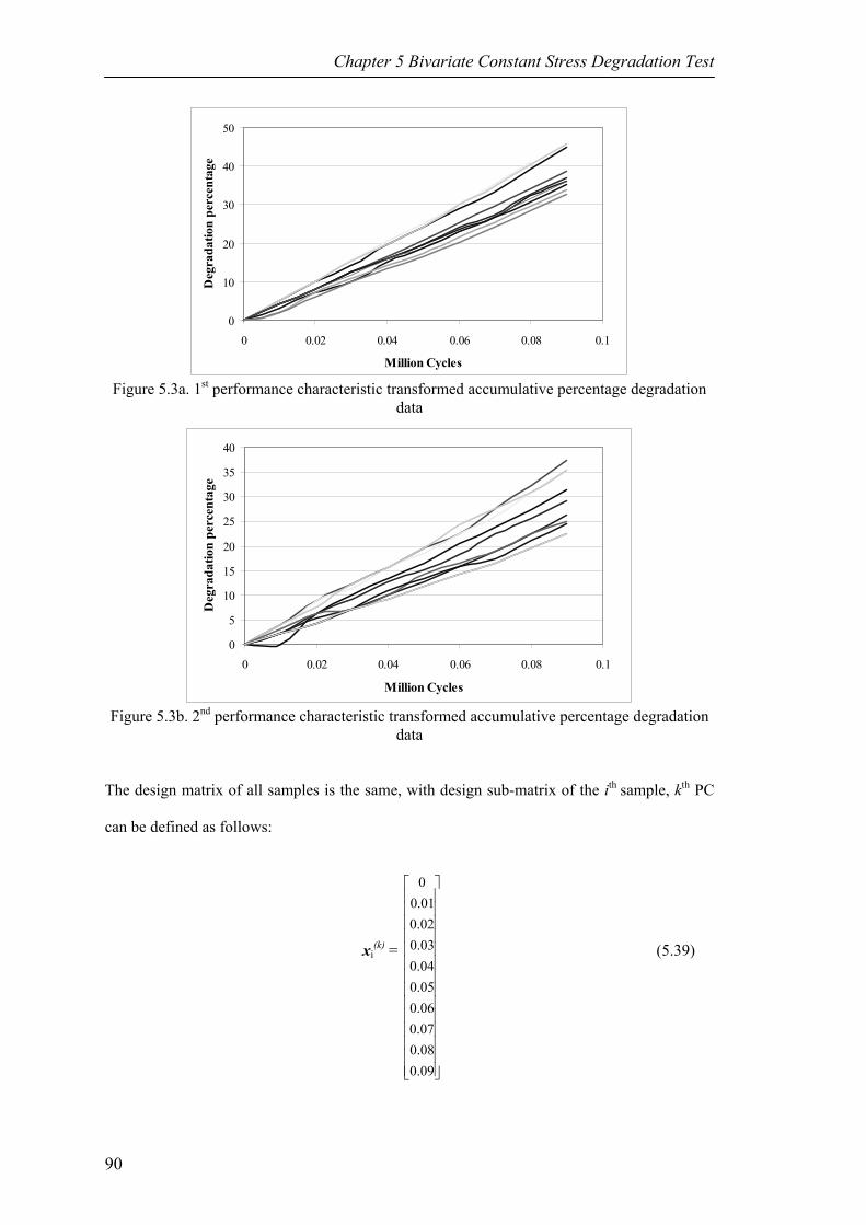
Chapter 5 Bivariate Constant Stress Degradation Test
0
10
20
30
40
50
0 0.02 0.04 0.06 0.08 0.1
Million Cycles
Deg
rada
tion
perc
enta
ge
Figure 5.3a. 1st performance characteristic transformed accumulative percentage degradation
data
0
5
10
15
20
25
30
35
40
0 0.02 0.04 0.06 0.08 0.1
Million Cycles
Deg
rada
tion
perc
enta
ge
Figure 5.3b. 2nd performance characteristic transformed accumulative percentage degradation
data
The design matrix of all samples is the same, with design sub-matrix of the ith sample, kth PC
can be defined as follows:
xi(k) = (5.39)
⎥⎥⎥⎥⎥⎥⎥⎥⎥⎥⎥⎥⎥⎥
⎦
⎤
⎢⎢⎢⎢⎢⎢⎢⎢⎢⎢⎢⎢⎢⎢
⎣
⎡
09.008.007.006.005.004.003.002.001.00
90

Chapter 5 Bivariate Constant Stress Degradation Test
And since from Figure 5.3 it can be concluded that the intersections of the graphs is zero, then
it can be assumed that the constant parameter of both PCs is zero. Therefore, the regression
parameter matrix can be written as:
= (5.40) ⎥⎦
⎤⎢⎣
⎡= )2(
)1(
ββ
β ⎥⎦
⎤⎢⎣
⎡
2
1
ββ
It is also assumed that the structure and values of the element of Zi are the same with Xi (Xi =
Zi). The random effect matrix bi has the same form with β. However, every sample has
different value of b while the value of β is the same for all samples.
Before defining the next elements of the model, the distribution functions of the marginal data
needs to be defined. Both PCs are assumed to follow Gamma distribution. It is chosen after
some assessment of possible distribution functions and also considering the possibility to
compare the result with the result of Model 3. The distribution of the random-effect
components is assumed to follow Normal distribution. Based on these assumptions, the
components of the covariance matrix can now be defined.
The within-unit covariance matrix is formed using estimated correlation matrix Γ1 which has
the following structure,
Γ1(2n×2n) =
⎥⎥⎥⎥⎥⎥⎥⎥⎥⎥⎥⎥⎥⎥
⎦
⎤
⎢⎢⎢⎢⎢⎢⎢⎢⎢⎢⎢⎢⎢⎢
⎣
⎡
100000
000
0010000100
000
000001
23
2
2
23
31
1
1
31
ρρρ
ρρρ
ρρρ
ρρρ
KKK
OOMOM
OOOMOM
MOOMO
KKK
KKK
OMOOM
MOMOOO
MOMOO
KKK
(5.41)
91

Chapter 5 Bivariate Constant Stress Degradation Test
Both PCs are assumed to have one-dependent correlation while for the between PCs
correlation it is assumed that realization of other PC at other measurement times does not have
any effect on degradation observation of a PC at certain measurement time. The within-unit
standard deviation matrix T1 is a diagonal matrix with its diagonal elements can be defined as,
Tij(k) = σk . f(xij
(k).β(k)); with i = j, and k = 1,2 (5.42)
Since the random-effects are assumed to be independent and follow Normal distribution, then
T2 and Γ2 can be expressed as follows,
T2 = ; Γ2 = (5.43) ⎥⎦
⎤⎢⎣
⎡
4
3
00σ
σ⎥⎦
⎤⎢⎣
⎡1001
Performing the estimation procedure given in sub-chapter 5.1.1, the unknown parameters of
the model are obtained and are presented in Table 5.3.
Table 5.3 Regression parameters estimation result of Model 1 PC Parameter Estimated value
β1 422.356 1 σ1 0.322 β2 311.806 2 σ2 0.192 σ3 54.999 σ4 44.999 Between PC ρ3 0.814
The random-effects parameters bi can then be calculated using (5.14). These are used to
predict the TTFs of both PCs which are listed in Table 5.4. In this table, the real TTF readings
of the two PCs taken from the test in line with scenario 1 can also be found. This will be
compared to the estimation result. Unfortunately, comparison of estimation result of second
scenario to the real data cannot be performed since we do not have the exact readings at the
threshold values of second scenario.
92

Chapter 5 Bivariate Constant Stress Degradation Test
Table 5.4 TTF data and prediction (in million cycles)
TTF reading at 1.6 inch
Scenario 1: TTF prediction
Scenario 2: TTF prediction
Sample
PC 1 PC 2 PC 1 PC 2 PC 1 PC 2 1 0.088 0.118 0.089 0.132 0.090 0.086 2 0.1 0.118 0.103 0.108 0.105 0.070 3 0.101 0.129 0.084 0.119 0.086 0.078 4 0.103 0.133 0.088 0.110 0.089 0.072 5 0.103 0.138 0.108 0.139 0.110 0.091 6 0.106 0.144 0.109 0.161 0.111 0.105 7 0.106 0.146 0.112 0.159 0.113 0.104 8 0.109 0.151 0.115 0.168 0.116 0.109 9 0.113 0.160 0.121 0.177 0.123 0.116 10 0.115 0.167 0.126 0.179 0.128 0.117
The TTF data of each PC is evaluated to determine which distribution function fits best to
each marginal TTF data. It is concluded that Inverse Gaussian distribution fits to represent the
both failure mechanisms TTF distribution functions. Using MLE, the predicted marginal TTF
data and marginal TTF distribution assumptions, the marginal TTF distribution parameters are
estimated. The predicted marginal distribution parameters are shown in Table 5.5. These
parameters are used to estimate the marginal PDF, CDF, and reliability of each failure
mechanism.
Table 5.5 Marginal TTF distribution parameters Failure Mechanism Parameters Scenario 1 Scenario 2
μ 0.105 0.107 1 (Inverse Gaussian) λ 5.922 6.016 μ 0.145 0.095 2 (Inverse Gaussian) λ 4.269 2.788
The system reliability of both scenarios of failure is estimated with two assumptions:
independent and dependent failure mechanisms. The system reliability with independent
failure mechanisms assumption is calculated by calculating the product of the marginal
reliability functions. To calculate the estimation of the system reliability with dependent
93

Chapter 5 Bivariate Constant Stress Degradation Test
failure mechanisms, copula function is needed. It is assumed that Frank copula can represent
the correlation between the two failure mechanisms and it can be written as:
( ) ( )( )( ) ⎟⎟
⎠
⎞⎜⎜⎝
⎛−
−−+−= −
−−
1111ln1, θ
θθ
θ θ eeevuC
vu
(5.44)
The u and v are the CDF of the first and second failure mechanisms respectively. The copula
parameter θ is estimated using IFM and information from the TTF prediction data. Despite
the different threshold values, the estimated copula parameter (using IFM) for both scenarios
is 9.10 which is equivalent to Kendall’s tau 0.64. If the Kendall’s tau is calculated directly
from the predicted TTF, both scenarios also produce the same measure of association.
However, it is different than the estimated measure of association calculated via IFM. This is
because dependency measurement with IFM approach is coupled with the copula function.
The marginal PDFs and reliability functions of scenario 1 are presented in Figure 5.4 and 5.5
respectively. In Figure 5.6, the estimated system reliability functions of scenario 1 are
presented. Figure 5.6 shows both independent and dependent system reliability based on the
real TTF data and predicted TTF data (from Model 1).
Figure 5.6 shows that the independent system reliability generally underestimate the system
reliability compared to the estimation with positive dependence assumption. This suggests
that in certain situation where correlation between failure mechanisms exists, dependency
assessment should be included in the system reliability modelling and assessment.
94

Chapter 5 Bivariate Constant Stress Degradation Test
Marginal PDF - Model 1, Scenario 1
0
10
20
30
40
50
60
0.025 0.075 0.125 0.175 0.225 0.275Million Cycles
PDF 1PDF 2PDF 1 - TTFPDF 2 - TTF
Figure 5.4. Marginal PDF of the bivariate fatigue crack analysis (PDF 1 and PDF 2) and real
TTF readings (PDF 1–TTF and PDF 2–TTF) Model 1 scenario 1
Marginal Reliability - Model 1, Scenario 1
0
0.2
0.4
0.6
0.8
1
0.05 0.075 0.1 0.125 0.15 0.175 0.2 0.225 0.25Million Cycles
Rel
iabi
lity
PC 1PC 2PC 1 - TTFPC 2 - TTF
Figure 5.5. Marginal reliability curves calculated from estimated TTF data (PC 1 and PC 2)
and real TTF readings (PC 1 – TTF and PC 2 – TTF) Model 1 scenario 1
System Reliability - Model 1, Scenario 1
0
0.2
0.4
0.6
0.8
1
0.05 0.075 0.1 0.125 0.15 0.175Million Cycles
Rel
iabi
lity
Independent
Frank Copula - TTFparameterTTF - Frank Copula
Figure 5.6. System reliability with independent and dependent assumption (Frank copula –
TTF parameter) and from real TTF readings using Frank copula (TTF-Frank copula), Model 1 scenario 1
95

Chapter 5 Bivariate Constant Stress Degradation Test
In the second scenario, the estimation result will not be compared to the estimation from TTF
readings because the real TTF readings for this scenario are not available. The results of the
estimation of the marginal PDF, marginal CDF and system reliability obtained from TTF data
predicted for PC 1 and 2 are shown in Figures 5.7, 5.8, and 5.9 respectively.
Marginal PDF - Model 1, Scenario 2
0
10
20
30
40
0.025 0.05 0.075 0.1 0.125 0.15 0.175
Million Cycles
PDF 1PDF 2
Figure 5.7. Marginal PDF of fatigue crack data Model 1 scenario 2
Marginal Reliability - Model 1, Scenario 2
0
0.2
0.4
0.6
0.8
1
0.05 0.075 0.1 0.125 0.15 0.175Million Cycles
Rel
iabi
lity
PC 1PC 2
Figure 5.8. Marginal reliability fatigue crack data Model 1 scenario 2
System Reliability - Model 1, Scenario 2
0
0.2
0.4
0.6
0.8
1
0.05 0.075 0.1 0.125 0.15 0.175
Million Cycles
Rel
iabi
lity
Independent
Frank Copula - TTFparameter
Figure 5.9. System reliability fatigue crack data Model 1 scenario 2
96

Chapter 5 Bivariate Constant Stress Degradation Test
The system reliability estimation with independent and dependent assumption in scenario 2
shows bigger difference then estimation in scenario 1. Since the other conditions and
definitions are the same, then the most probable cause is different threshold values definition
in scenario 1 and 2. This shows that when the failure mechanisms are correlated,
simplification of the model using independent model will lead us to the wrong conclusion of
system reliability.
5.4.2. Model 2 Example
The same data is modelled and evaluated using Model 2. In this analysis, marginal
degradation distribution function of each failure mechanism and its parameter(s) are estimated
in the beginning of stage 1 of Model 2. The distribution evaluation is done not on the
transformed percentage data in Table 5.2 but instead it is done on the accumulative percentage
degradation data compared to the initial measurement. The PCs observation data in
cumulative percentage crack measurement is shown in Table 5.6. This data is also presented
in the form of graphs as shown in Figure 5.10.
For each marginal data at each measurement time, probability distribution analysis is
performed. Based on this analysis and to show that the model is working with different
marginal distributions, it is decided that Lognormal and Weibull distributions will be used to
illustrate the first and second marginal degradation distributions respectively. With these
assumptions, the marginal distribution parameters at all measurement times are estimated.
97

Chapter 5 Bivariate Constant Stress Degradation Test
Table 5.6. Cumulative crack percentage compared to the initial measurement (%) Sample Million
Cycles PC 1 2 3 4 5 6 7 8 9 10 0 1 0 0 0 0 0 0 0 0 0 0
0.01 5.56 4.44 4.44 4.44 4.44 4.44 4.44 3.33 2.22 2.22 0.02 11.11 8.89 8.89 8.89 8.89 8.89 8.89 7.78 7.78 6.67 0.03 16.67 14.44 14.44 14.44 14.44 14.44 13.33 11.11 12.22 11.11 0.04 24.44 20 20 18.89 18.89 18.89 18.89 17.78 16.67 15.56 0.05 32.22 26.67 25.56 24.44 24.44 24.44 23.33 23.33 21.11 20 0.06 41.11 34.44 32.22 32.22 32.22 31.11 30 30 27.78 25.56 0.07 50 42.22 40 38.89 37.78 36.67 36.67 36.67 34.44 32.22 0.08 64.44 52.22 50 48.89 48.89 47.78 46.67 44.44 42.22 40 0.09 82.22 63.33 62.22 58.89 58.89 56.67 56.67 54.44 51.11 48.89
0 2 0 0 0 0 0 0 0 0 0 0
0.01 0 3.33 2.22 3.33 2.22 2.22 3.33 2.22 2.22 2.22 0.02 6.67 7.78 7.78 6.67 6.67 5.56 6.67 4.44 4.44 4.44 0.03 11.11 11.11 10 11.11 10 7.78 7.78 7.78 7.78 7.78 0.04 15.56 14.44 14.44 14.44 14.44 11.11 11.11 12.22 10 10 0.05 20 18.89 17.78 18.89 17.78 14.44 16.67 15.56 13.33 13.33 0.06 25.56 22.22 22.22 24.44 22.22 18.89 20 18.89 16.67 16.67 0.07 31.11 28.89 26.67 28.89 28.89 23.33 23.33 21.11 20 20 0.08 37.78 35.56 33.33 33.33 34.44 28.89 28.89 26.67 24.44 24.44 0.09 45.56 43.33 40 40 41.11 35.56 33.33 32.22 28.89 28.89
It is assumed that the parameter σ of the first PC is not a function of time because there is no
apparent trend of the σ estimations over time. Therefore, the average of estimated σ collected
during the test will be used. On the contrary, the estimated parameter μ of the first PC is
assumed to be a function of time. GLM is performed to find the regression parameter of μ.
The shape parameter β of the second PC is also assumed to be not a function of time (for the
same reason as σ) while the scale parameter α is a function of time.
98

Chapter 5 Bivariate Constant Stress Degradation Test
0
10
20
30
40
50
60
70
80
0 0.02 0.04 0.06 0.08 0.1
Million Cycles
Deg
rada
tion
perc
enta
ge
Figure 5.10a. Performance characteristic 1 cumulative percentage degradation data
0
5
10
15
20
25
30
35
40
45
0 0.02 0.04 0.06 0.08 0.1
Million Cycles
Deg
rada
tion
perc
enta
ge
Figure 5.10b. Performance characteristic 2 cumulative percentage degradation data
The GLM model of the parameters μ and α of the first and second PC marginal distribution
can be written as follows,
E(μ) = β11 + β12.t
Var(μ) = σ12. Γ1
E(α) = β21.t
Var(α) = σ22. Γ2 (5.45)
The result of the GLM estimation is presented in Table 5.7. The distribution parameters in
Table 5.7 are used to estimate the marginal reliability of the system at time t by utilizing the
marginal distribution function (F(k)(t)), threshold value definition, and Equation (5.4). This is
carried out for both failure scenarios.
99

Chapter 5 Bivariate Constant Stress Degradation Test
Table 5.7. Estimated marginal degradation distribution parameters of fatigue crack data Model 2 (t in million cycles)
PC Parameter Estimated value/regression functionμ ≈1.79 + 26.39 t 1 σ 0.129 α ≈ 394.712 t for t > 0 2 β 7.535
The estimation of copula parameter is done using IFM with assumption that Frank copula can
represent the dependency between the PCs. The Frank copula density function (c(u, v)) for
bivariate data can be written as:
( ) ( ) ( )( )( )( ) ([ ]) 2111
1,−+−−
−−=
−−−
+−−
θθθ
θθθ
eeeeevuc
vu
vu
(5.46)
It is found that the Frank copula parameter (θ) value is 4.02 or equal to Kendall’s tau of 0.39
for both failure scenarios. The θ is assumed to have a fix value which is the average of the
estimation taken at all measurement times because the estimation result shows no strong
evident of particular trend.
In Figures 5.11, 5.12, and 5.13 the marginal PDF, marginal reliability and system reliability
obtained from Model 2, scenario 1, are presented together with the estimation based on the
TTF observation data. It is obvious that the estimation of marginal PDF and reliability of the
second PC are significantly different from estimation from TTF observation. And these result
in considerably different system reliability estimation compared to the marginal reliability
estimated from TTF observation. A possible cause is the regression model for the Weibull
parameter α in (5.45) does not accurately represent its function over time. This is an
indication that it is important to choose the best possible model to describe how the
distribution parameter changes over time. This will be discussed in the last sub-chapter of this
chapter.
100

Chapter 5 Bivariate Constant Stress Degradation Test
Marginal PDF - Model 2 scenario 1
0
1020
3040
50
6070
80
0.05 0.1 0.15 0.2 0.25 0.3 0.35Million cycles
PC 1PC 2TTF 1 - observationTTF 2 - observation
Figure 5.11. Marginal PDF fatigue crack data Model 2 scenario 1
Marginal Reliability - Model 2 scenario 1
0
0.2
0.4
0.6
0.8
1
0 0.05 0.1 0.15 0.2 0.25 0.3 0.35 0.4
Million cycles
Rel
iabi
lity
PC 1 - model 2PC 2 - model 2PC 1 - TTFPC 2 - TTF
Figure 5.12. Marginal reliability fatigue crack data Model 2 scenario 1
System Reliability - Model 2 scenario 1
0
0.2
0.4
0.6
0.8
1
0.07 0.08 0.09 0.1 0.11 0.12 0.13 0.14
Million Cycles
Rel
iabi
lity
Independent
Dependent Model 2
From TTF
Figure 5.13. System reliability with independent and dependent assumption (Dependent Model
1) and from real TTF readings using Frank copula (From TTF data), Model 2 scenario 1
101

Chapter 5 Bivariate Constant Stress Degradation Test
Marginal PDF - Model 2 scenario 2
01020304050607080
0.05 0.075 0.1 0.125 0.15 0.175 0.2Million cycles
PC 1PC 2
Figure 5.14. Marginal PDF fatigue crack data Model 2 scenario 2
Marginal Reliability - Model 2 scenario 2
0
0.2
0.4
0.6
0.8
1
0.05 0.075 0.1 0.125 0.15 0.175 0.2
Million Cycles
Rel
iabi
lity
PC 1PC 2
Figure 5.15. Marginal reliability fatigue crack data Model 2 scenario 2
System Reliability - Model 2 scenario 2
0
0.2
0.4
0.6
0.8
1
0.075 0.08 0.085 0.09 0.095 0.1 0.105 0.11 0.115
Million Cycles
Rel
iabi
lity
IndependentDependent Model 2
Figure 5.16. System reliability Model fatigue crack data 2 scenario 2
102

Chapter 5 Bivariate Constant Stress Degradation Test
Another important observation is the striking similarity of the system reliability estimations
with independent and dependent assumption. This may be caused by the copula parameter
value which is close to zero.
The results of scenario 2 are presented in Figures 5.14, 5.15 and 5.16. These figures confirm
our preliminary hypothesis that different failure scenarios of the same degradation data will
give different assessment result of the system reliability. The analysis of scenario 2 results in
marginal reliability functions that overlaps each other while the first scenario shows two
marginal reliability functions that do not crossed each other. The dependent system reliability
of scenario 2 is also considerably different from its independent system reliability compared to
the result of scenario 1. Therefore, it is important to study the effect of the threshold value
definition to the system reliability.
5.4.3. Model 3 Example
Here, the GLM-PA approach is used. The model can be written similar to (5.38) without the
random-effect components as follows,
E(Y) = f(X.β) = ( )β.10090
X−
Var(Y) = V = T.Γ.T (5.47)
Another difference to Model 1 example is the structure of X.β. Here, the constant parameter
of the simple linear function used to represent the function of degradation readings exists (i.e.
β11, β21 ≠ 0). Meanwhile, the correlation matrix has sub-matrices of the first and second PC
with one-dependent structure and sub-matrix of between PCs correlation with diagonal
structure. Similar to Model 1, both PCs are assumed to follow Gamma distribution function.
103

Chapter 5 Bivariate Constant Stress Degradation Test
After performing the estimation procedure, the result is obtained and the summary is presented
in Table 5.8. The mean (E(Y)) and variance (V) of each PC can be arranged to estimate the
marginal degradation distribution parameters. The relationships between the GLM
components and Gamma distribution parameters at jth measurement time can be expressed as
follows,
Scale parameter = θj
(k) = σk2. )(k
jY
Shape parameter = k = 21 kσ (5.48)
Table 5.8. Estimated GLM components of Model 3 (t in million cycles) PC Component Estimated value/regression function
X(k).β(k) ≈ -0.171 + 423.54t 1 σ1 0.116 X(k).β(k) ≈ -0.318 + 316.637t 2 σ2 0.194
Frank copula is chosen to model the between PCs dependency. Using IFM the copula
parameter is estimated. The copula parameter is assumed not a function of time and its
estimation is 32.37, which is equal to Kendall’s tau of 0.88. This is considerably higher than
correlation estimation in Models 1 and 2.
Based on these estimations, the marginal and system reliability functions are evaluated for
both failure scenarios. Independent system reliability is also obtained and compared to its
dependent counterpart. Figures (5.17) – (5.19) show the results for scenario 1, while Figures
(5.20) – (5.22) show the results for scenario 2.
It can be seen that the result of Model 3 scenario 1 is more similar to the result of Model 1.
And compared to Model 2, the 2nd PC of Model 3 is closer to the estimation derived from real
TTF observations. In addition, the independent and dependent system reliability functions of
Model 3 show bigger difference from those in Model 2.
104

Chapter 5 Bivariate Constant Stress Degradation Test
Marginal PDF - Model 3 scenario 1
0
10
20
30
40
50
60
0 0.05 0.1 0.15 0.2 0.25 0.3Million cycles
PC 1 - model 3PC 2 - model 3PC 1 - TTFPC 2 - TTF
Figure 5.17. Marginal PDF fatigue crack data Model 3 scenario 1
Marginal Reliability - Model 3 scenario 1
0
0.2
0.4
0.6
0.8
1
0 0.05 0.1 0.15 0.2 0.25 0.3
Million Cycles
Rel
iabi
lity
PC 1 - model 3PC 2 - model 3PC 1 - TTFPC 2 - TTF
Figure 5.18. Marginal Reliability fatigue crack data Model 3 scenario 1
System Reliability - Model 3 scenario 1
0
0.2
0.4
0.6
0.8
1
0.025 0.05 0.075 0.1 0.125 0.15 0.175
Million cycles
Rel
iabi
lity
Independent - model 3Frank copula - model 3TTF - Frank copula
Figure 5.19. System reliability fatigue crack data Model 3 scenario 1
105

Chapter 5 Bivariate Constant Stress Degradation Test
Marginal PDF - Model 3 scenario 2
0
5
10
15
20
25
30
35
0 0.05 0.1 0.15 0.2 0.25Million cycles
PC 1 - model 3PC 2 - model 3
Figure 5.20. Marginal PDF fatigue crack data Model 3 scenario 2
Marginal Reliability - Model 3 scenario 2
0
0.2
0.4
0.6
0.8
1
0 0.05 0.1 0.15 0.2 0.25
Million Cycles
Rel
iabi
lity
PC 1 - model 3PC 2 - model 3
Figure 5.21. Marginal reliability fatigue crack data Model 3 scenario 2
System Reliability - Model 3 scenario 2
0
0.2
0.4
0.6
0.8
1
0 0.025 0.05 0.075 0.1 0.125 0.15 0.175
Million cycles
Rel
iabi
lity
Independent - model 3Dependent - model 3
Figure 5.22. System reliability fatigue crack data Model 3 scenario 2
106
Chapter 5 Bivariate Constant Stress Degradation Test
The analysis result of scenario 2 somehow shows that the marginal reliability of 2nd PC started
noticeably below 1. This affects the system reliability which also started not from 1 but from
less than 1. This may be caused by combination of some factors, such as marginal distribution
definition, regression modelling, and threshold value definition. This can also be interpreted
that given the degradation test observation of the second PC there is some probability of the
existence of early failure which does not captured by Model 2. This phenomenon also appears
in Wang and Coit (2004), but they did not discuss this further.
Another trial using Model 3 with the data modelled as a function of simple linear function
without constant parameter is also performed. The result of the second trial using Model 3 on
the same data is very similar to the first trial where the constant parameter is allowed to have
other value than zero. This means that the constant parameter in the regression model may not
be necessarily included.
5.5. Discussion of the Bivariate Models
Following the presentation of the proposed models and their implementation on the fatigue-
crack data, it can be concluded that the first bivariate model is suitable when,
1. The link function between the components of the degradation data regression model and
the marginal degradation distribution parameters cannot be established. Therefore, the
marginal reliability cannot be estimated from the marginal degradation distribution (recall
Equation (5.4)),
2. Because of the difficulty to estimate the marginal degradation distribution parameters, the
failure mechanisms dependency should be estimated using IFM on the predicted TTF data.
This is a consequent of IFM approach which needs the CDF estimation of the data as
input,
3. And when there is need to obtain the predicted TTF data.
107

Chapter 5 Bivariate Constant Stress Degradation Test
Meanwhile, Model 2 should be used in the following situations,
1. The marginal degradation distribution function is not a member of the exponential family
and/or it is not possible to construct the link function between its parameter and the
components of GLM,
2. There is an interest to evaluate the structure of between PCs dependency and there is
possibility that it is a function of time,
3. If there are more than one set of bivariate degradation data, each with certain number of
samples, tested with the same test conditions. In this case, data of each degradation test
will give us one set of input for Model 2.
As for Model 3, it should be used in the following conditions,
1. The value of marginal degradation distribution parameter(s) can be concluded from the
components of the degradation data regression model,
2. There is an interest to evaluate the structure of between PCs dependency and there is
possibility that it is a function of time,
3. There is an interest to evaluate the structure of the cross-correlation sub-matrix and
analyze the effect of measurements of the other PC taken at different measurement time to
a particular observation.
These conclusions are inferred from the descriptions of the models. Besides these, analysis
based on the implementation examples is also carried out on the three examples. This will
give more insights on the characteristics of the models and possible improvements and
investigations.
By examining the three models, it can be suggested that the result of the univariate analysis
plays an important role in the bivariate analysis. This was shown by the results of Model 2
and 3. The marginal degradation data in those examples was modelled by different marginal
108

Chapter 5 Bivariate Constant Stress Degradation Test
distribution functions on purpose. It was shown in Sub-chapters 5.4.2 and 5.4.3 that modelling
the same univariate data with different distribution functions will result in different reliability
conclusion even though the same copula function is used to represent the between PCs
dependency. Therefore, it is important to choose the most suitable univariate distribution to
model the marginal data.
In relation to the marginal degradation modelling of Model 2, extra attention should be given
in choosing the transformation of the distribution parameters, their regression function and the
link function. This should be done carefully while paying attention to the characteristics of the
marginal distribution functions. For example, if Gamma distribution is chosen to model the
marginal degradation data, the regression function of its distribution parameters should only
give positive value estimation in addition to keep the marginal CDF monotone over time.
Besides the choice of the marginal distribution function, the system reliability is also affected
by its marginal failure mechanisms. It was shown in the three examples, if the marginal
reliability functions do not cross each other as in the scenario 1 of the three models, the most
left marginal reliability (which has more “severe” failure” mechanism) has stronger effect on
the system reliability. Furthermore, the system reliability is closer to the more “severe”
marginal reliability.
Another point that needs our attention is the effect of the threshold value definition. The
results of the two failure scenarios analysis have shown that even though the data is analyzed
using the same model, different failure scenario (i.e. threshold value definitions), the results
could be quite different. Therefore, if there are different experts' opinions on the threshold
value definition, extra analysis is needed to avoid making under- or over-estimate system
reliability.
109
Chapter 5 Bivariate Constant Stress Degradation Test
The last discussion is on the result of Model 3 scenario 2. It was shown that the marginal
reliability of the second PC and the system reliability start not from 1 but from some values
below 1. This phenomenon also found in Wang and Coit (2004). This is the consequence of
the reliability definition in Equation (5.4) combined with the threshold value definition. When
degradation measurements are represented by a distribution function and the threshold value
definition is located at the location where the CDF of the degradation data at t = 0 is not equal
to 1, then the reliability will start from a value below 1. This may be interpreted as the
possibility of the existence of weak population or can also be used to explain the occurrence of
some No-Fault-Found (NFF) incidents where products fail in the beginning of their life
without obvious failure cause. Further study is needed to justify this as explanation of early
failure probability in a degraded system related to the PCs of the system.
110

Chapter Six
Multivariate Constant-Stress Degradation Test
In chapter five, three reliability models and analysis methods for bivariate CSDT data has been
proposed and implemented to fatigue-crack data from Bogdanoff and Kozin (1985). The
performance characteristics (PCs) of the system are related to the two main failure
mechanisms of the system and the system is considered failed if at least one of the PCs first
crosses its threshold value. It has been shown that it is possible to estimate reliability of a
bivariate degradation system without forcing the assumption of independent PCs. It is
important to take the between PCs dependence into account because ignoring it may lead us to
different reliability estimation while the dependency justly exists. And since the components
of a system are likely to have common shared factors, the failure mechanisms are likely to
have some degree of dependency. And this has been incorporated into the proposed bivariate
models together with more flexibility in marginal distribution choices and inclusion of serial
correlation of a PC.
111

Chapter 6 Multivariate Constant Stress Degradation Test
A natural extension of a bivariate CSDT model is a multivariate CSDT model. It is useful to
analyze and estimate reliability of a multivariate degraded system. This need can be justified
by the increasing number of functions/aspects in modern systems/products. For example:
LED lighting system consists of arrangement of many LED components is considered failed if
either the cumulative illumination degradation or the cumulative colour changes or the
accumulative number of dead LED components are above certain levels. For these cases,
multivariate CSDT model is needed to evaluate the system reliability.
The published works (i.e. Crk (2000), Huang and Askin (2003), Zhao and Elsayed (2004),
Wang and Coit (2004), Bagdonavicius et.al. (2004), and Xu and Zhao (2005)) that address
multivariate degradation data modelling for industrial purposes utilize independence
assumptions of the PCs, multivariate Normal distribution for the joint distribution or the use of
same marginal distribution functions. These assumptions should be relaxed as what has been
done in chapter five. Yet, the models in chapter five only accommodate bivariate data.
Hence, the multivariate extension will be explored in this chapter to provide alternative
models for multivariate CSDT data.
The models in chapter five generally can be seen as two-stage models with different details:
univariate and bivariate stages. The multivariate extension of the models will also have two
stages. There is almost no significant change in the univariate stage in the multivariate model.
However, more attention is needed when performing second stage of the multivariate analysis.
The important tool of the second stage is copula function. The copula functions used in
chapter five are bivariate copula. This arises some questions: (1) how to derive the
multivariate form of copulas, (2) how do we interpret the multivariate copulas and their
parameter(s) with respect to the dependency between the failure mechanisms, and (3) is the
same estimation method can be used to estimate the multivariate copula parameter(s).
Additional thing that may be interesting is how to simulate a multivariate time series data with
112

Chapter 6 Multivariate Constant Stress Degradation Test
more than one sample unit. Some of these issues and the multivariate CSDT model will be
discussed in this chapter.
In summary, the topics that will be included in the discussion in this chapter are:
1. Multivariate CSDT model development to analyze the multivariate degradation data and
evaluate system reliability by taking into account possible between PCs dependence
assumption, different distribution families of marginal data, and possible serial correlation
of the marginal degradation observation,
2. Discussion on possible multivariate copulas for system reliability estimation purpose for
industrial use,
3. Estimation method of the unknown parameters in the model including constraints and
possible interpretation of the copula parameters in the industrial problems.
The multivariate models that will be proposed in this chapter are the extension of the bivariate
models in chapter five. These will be discussed in the section 6.2 with assumption that the
multivariate copulas are known. Before this discussion, in sub-chapter 6.1 the multivariate
copula functions and further discussion of the possible choices for industrial purposes
including estimation methods and copula parameters' interpretation is presented.
6.1. Multivariate Copula Functions
Since the multivariate CSDT models that will be presented in this chapter are natural
extension of the bivariate CSDT models in chapter five, it is obvious that copula functions
play an important role in the model. Therefore, the discussion on the multivariate copulas will
first be introduced before discussion of their utilization in the multivariate CSDT models.
113

Chapter 6 Multivariate Constant Stress Degradation Test
Multivariate copulas will be used to represent the dependence structure between PCs (or
TTFs) and relationships between the marginal distributions and their joint distribution.
Therefore, copulas can be used to substitute joint distribution function needed to assess system
reliability. Using this, the marginal distributions may follow different distribution families.
There are some issues surrounding construction of multivariate copulas for multivariate CSDT
models, such as:
1. Construction method of the multivariate copulas,
2. Interpretation of the multivariate copulas' parameter,
3. Trade-off between difficulty of computation and type and efficiency of dependency
information needed,
4. Range of dependency that is accommodated by the multivariate copulas model.
There are some known construction methods of multivariate distributions that are also valid
for multivariate copulas construction, for examples mixtures, stochastic representations, limits,
etc. Some of the multivariate copula families are extension of their bivariate counterparts (and
have univariate marginals) and some are constructed from bivariate marginals or lower order
multivariate marginals. These construction methods may have different motivations,
properties, and difficulty levels which will not be discussed in this thesis. We will instead
focus on the possible usage in modelling multivariate degradation data and the fitness to
reliability problems.
There is no current method that can deliver multivariate copulas that satisfy all desirable
properties of multivariate distribution functions yet. These properties are considered in
multivariate model construction and choosing the suitable function for certain multivariate
CSDT problems. They are (Joe, 1997):
1. Interpretability of the multivariate distribution,
114

Chapter 6 Multivariate Constant Stress Degradation Test
2. The closure property under the taking of margins, in particular the bivariate margins
belonging to the same parametric family,
3. A flexible and wide range of dependence,
4. A closed-form representation of the CDF and PDF or if not, at least computationally
feasible to work with.
So far, no known parametric multivariate distribution family can satisfy all of the above
requirements. The closest one with properties 1 - 3 is multivariate Normal (MVN)
distribution. However, it has no closed-form distribution function and all of the marginal
distributions required to be Normal distribution. The copula form of MVN is multivariate
Gaussian copula (MGC) function. It is more flexible than MVN distribution – different
marginal distributions are possible – and has a wide range of dependency. Clemen and Reilly
(1999) explore and discuss the utilization of MGC to assess correlation in decision and risk
analysis. However, if tail dependency analysis is important, MGC is not the correct tool to use
because it does not have tail dependency.
As suggested by Nelsen (1999) constructing multivariate copula is difficult and few
procedures have p-dimensional copulas analogs. One of the construction procedures that often
succeed for the class of Archimedean copulas is the extension of the bivariate copula
construction by treating the margins (F(1)(y(1)) and F(2)(y(2))) of the usual 2-copula (C(F(1)(y(1)),
F(2)(y(2))) as an p1 and p2 dimensional distribution functions respectively. However, with this
construction all bivariate margins should be the same family and the multivariate form has
only p – 1 bivariate margins from p univariate margins. That means not all of the dependence
structures of the failure mechanisms can be assessed.
Two families of established multivariate copulas will be considered in the following
discussion. They are Elliptical copulas and Archimedean copulas. These were chosen by
115

Chapter 6 Multivariate Constant Stress Degradation Test
bearing in mind the need of simplicity of the model, minimize computation burden of the
estimation, possible interpretation of the model, and previous studies on multivariate copulas.
6.1.1. Multivariate Elliptical Copulas
Elliptical copulas are copula forms of the elliptical distributions (Embrechts et.al., 2001).
Elliptical distributions, especially Normal distribution and Student-t distribution, have been
used extensively in many areas. Even though these distributions do not have closed-form
CDF, their direct interpretation of their parameters and easy extension to multivariate forms
are some of the reasons that made them popular. Random variable which is distributed
according to the Elliptical distributions family has a special stochastic representation. Let Y as
n-dimensional random variable which follows Elliptical distribution family (En(μ,∑,φ)) and R
a non-negative random variable independent of U which is a uniformly distributed random
vector with {u ∈[-1,1]r : u =1} with rank (∑) = r ≤ n, the elliptical random vector can be
written as,
Y = μ + R Σ U (6.1)
Besides normal and Student-t distributions, other examples of Elliptical distribution family are
elliptical distribution (which is a special class of Elliptical family), sub-Gaussian α-stable and
Cauchy distributions. In this thesis, two multivariate elliptical copulas derived from Normal
distribution and Student-t distribution will be discussed.
6.1.1.1. Multivariate Gaussian Copula
As pointed out by Clemen and Reilly (1999), Gaussian copula has a good potential to
represent dependency between its univariate margins. This is facilitated by its correlation
116
Chapter 6 Multivariate Constant Stress Degradation Test
matrix R which has basically similar representation to the MVN distribution. The
characteristics of MGC are:
1. MGC can be modelled with different marginal distributions (other than Normal
distribution) while MVN cannot ,
2. MGC permits the use of any positive semi-definite correlation matrix,
3. The existence of relationship between measure of association (Kendall's tau or Spearman's
rho) to product-moment correlation that is needed for MGC model,
4. Conditional densities can be calculated easily when necessary.
On the other hand there are some disadvantages of MGC such as: it does not have closed-form
density function, it cannot be evaluated when the PCs’ correlation assessment results in non-
positive-definite correlation matrix R and when the problem is mixture distributions, MGC
may not give the best joint probability function assessment.
Let assume that we have y(k) (k = 1,2,…,p) correspond to p PCs. The joint probability density
function of MGC at particular measurement time t can be written as:
( )*)()1( ,,..., Rtyyf p =
( ) ( )tyftyf pp )()()1()1( ××K
( )[ ] ( )[ ]( ) ( )IR −×ΦΦ−× −−− 1)()(1)1()1(1 ,,exp{ tyFtyF ppK
( )[ ] ( )[ ]( ) 21
/}2/,, )()(1)1()1(1 RTpp tyFtyF −− ΦΦ× K (6.2)
Where:
R* = matrix of between PCs measure of associations
R = matrix of product-moment correlation between PCs, corresponded to R*
I = identity matrix (p × p)
Φ = Normal distribution cumulative density function
117

Chapter 6 Multivariate Constant Stress Degradation Test
The density of the margins is analyzed and estimated separately from the multivariate model.
Therefore, the marginal models are robust from misspecification of the multivariate
dependency model. Unfortunately, this also means that the marginal estimations do not make
the most of available multivariate dependency information. Nonetheless, this will be made up
by the advantage of inference function of marginal (IFM) i.e. less computation burden with
relatively high efficiency.
The components of R* are obtained from measure of association estimation between PCs with
1s as the diagonal components. This can be done for each measurement time and each
bivariate correlation of the multivariate data. There are two possible approaches for
estimation the off-diagonal components of the correlation matrix R:
1. Estimate the measure of associations of between-PCs and transform these estimation into
product-moment correlation matrix (R),
2. Using IFM on the part of log-likelihood function related to Gaussian copula density,
estimate the elements of matrix R.
In the first approach, estimation of measure of association has to be carried out for all possible
combination of bivariate dependency. With assumption that the cross-correlation elements do
not change over time, calculate (k1 < k2 and 1 ≤ k1 < k2 ≤ p) at each measurement time
and calculate the average. Use correlation formula between measure of association and
product-moment correlation to calculate the estimated , which are the elements of matrix
R. The conversion formula for Kendall’s tau is:
*2,1 kkr
2,1 kkr
2,1 kkr = ⎟⎟⎠
⎞⎜⎜⎝
⎛
2sin
*2,1 kkrπ = ⎟⎟
⎠
⎞⎜⎜⎝
⎛2
sin 2,1 kkπτ (6.3)
118

Chapter 6 Multivariate Constant Stress Degradation Test
In the second procedure, a log-likelihood function of the Gaussian copula density is needed.
The copula parameters are estimated from part of log-likelihood function independently of the
marginal parameters. The copula density function of MGC is:
( ) ( )( )( )tyFyFc pp)()1()1( ,,K = ( ){ }2
1
2/exp 1
RIR ζζ −− −T
(6.4)
Where ζ = ( )( ) ( )( )( Tpp tyFyF )()(1)1()1(1 ,, −− ΦΦ K ) , is the inverse of cumulative standard
Normal distribution of the degradation readings given measurement time = t. To estimate the
copula parameters, maximize log-likelihood of (6.4) with respect to R. These parameters will
be used to assess the reliability of the multivariate degraded system.
MGC with respect to the multivariate PCs at measurement time t can be written as,
C(F(1)(y(1)|t),..., F(p)(y(p)|t)) = Φ(Φ-1(F(1)(y(1)|t)),..., Φ-1(F(p)(y(p)|t))) (6.5)
This definition will be used in the system reliability estimation. In this case, MGC represent
the pair-dependency of the data. Note that in the case of multivariate extension of Model 1,
the random variables of the MGC are not the PCs’ measurements but the predicted TTFs.
The advantages of Gaussian copula have been noticed by some researchers and used in their
studies. Besides Clemen and Reilly (1999) who used Gaussian copula for multivariate data for
decision and risk analysis, Edgeworth (1898) also implemented the use of non-Normal
marginal distributions with bivariate Normal distribution dependence structure to describe
their joint distribution.
119

Chapter 6 Multivariate Constant Stress Degradation Test
6.1.1.2. Multivariate Student-t Copula
Multivariate Student-t copula is generated from the Student-t distribution. It is a probability
density function that was discovered by William S. Gosset and used for estimation problem of
normally distributed population when the sample size is small. The Student-t copula also has
linear correlation matrix R as in the MGC. The Student-t copula has the similar characteristics
as MGC except that it has upper and lower tail dependence, while MGC does not have.
The Student-t copula for degradation measurement random variables (Y) can be written as,
C(F(1)(y(1)|t),..., F(p)(y(p)|t)) = Tυ(tυ-1(F(1)(y(1)|t)),..., tυ-1(F(p)(y(p)|t))) (6.6)
In (6.6), tυ is the univariate standard Student-t distribution with υ degree of freedom. The
copula density of Student-t copula of p random variables can be expressed as,
( ) ( )( )( )tyFyFc pp)()1()1( ,,K =
( ) Rp
p
υπυ
υ
⎟⎠⎞
⎜⎝⎛
⎟⎠⎞
⎜⎝⎛ +
2
2
Γ
Γ ( ){ } 21
1
pT
+−−
⎟⎟⎠
⎞⎜⎜⎝
⎛ −+
υ
υζζ IR (6.7)
It should be noted, that because of the radial symmetry the upper and lower tail dependence of
two univariate components of the Student-t copula are equal. This tail dependence at certain
measurement time t can be expressed by the following equation (Embrechts et.al., 2001),
λk1,k2 = 2tυ+1 ⎟⎟
⎠
⎞
⎜⎜
⎝
⎛
+
−+
2,1
2,1
1
11
kk
kk
ρ
ρυ ; k1 ≠ k2 (6.8)
In Equation (6.8) the tail dependence between k1th and k2th PCs is expressed as a function of
the degree of freedom and off diagonal component of matrix R. These tail dependences go to
zero as the degree of freedom tends to infinity. This is logical since Student-t distribution
becomes closer to Normal distribution as the degree of freedom increases.
120

Chapter 6 Multivariate Constant Stress Degradation Test
It can be concluded that both MGC and multivariate Student-t copula can be applied easily to
evaluate the dependence structures between their two univariate margins while giving the
overall relationships between the multivariate distribution function and its margins. However,
the correlation matrix R should be positive semi-definite for both copulas and there is no tail
dependence for MGC. The positive semi-definite requirement of matrix R gives a constraint
in performing simulation (including with the simulation procedure in appendix A). An
alternative simulation procedure which does not need positive semi-definite correlation matrix
can be performed using Vines, which will not be discussed in this thesis. This is introduced by
Bedford and Cooke (2002) and appears in Kurowicka and Cooke (2006). In addition, note that
the upper and lower tails of Student-t copula are the same because of radial symmetry.
6.1.2. Multivariate Archimedean Copulas
The other candidate for the multivariate model is Archimedean copula. This class has gained
its popularity because of easiness of construction, the availability of great variety of families in
this class, and the nice properties of the families in this class (Nelsen, 1999). To extend this
the copulas functions in this class into multivariate copulas some construction methods can be
used. However, to choose which method to be used, we should bear in mind our purposes
which are:
1. To estimate system reliability at each stage (time) of the system’s life,
2. To include at least general dependency between PCs in the model.
There are some construction methods that can be used to extend bivariate Archimedean
copulas to multivariate copulas. However, there are some constraints for the multivariate
copulas compared to their bivariate form, such as:
1. The dependency range may be not as wide as in its bivariate form (i.e. not covering [-1,1]
measure of association range,
121

Chapter 6 Multivariate Constant Stress Degradation Test
2. The copula parameters related to the dependency between the random variables may not
be available for all pairs of the random variables when the multivariate form is constructed
using certain method,
3. In some cases, all lower dimension multivariate copulas have to be originated from the
same family to the higher dimension and more additional calculation steps are needed as
the dimension of the multivariate copula increases.
Considering these, the amount of further studies needed, and the need to assess system
reliability, an exchangeable multivariate copula model may be satisfying enough since even
more complicated models still cannot give complete dependence representations of all
marginal combinations. In the exchangeable multivariate copula model, the copula parameter
is seen as a general dependence parameter.
The exchangeable multivariate Archimedean copulas have a simpler representation than
multivariate copulas constructed using other methods, but there are some conditions that must
be satisfied. The following Archimedean k-copula functions are generated from one-
parameter family and also have one-parameter in their multivariate form. Therefore, the
copula parameter represents the general multivariate dependency. Nevertheless, it still serves
our goal in assessing system reliability with dependent assumption.
The following theorem, which is the necessary and sufficient conditions that are needed for
generating Archimedean k-copulas (k ≥ 2) from a strict generator ϕ , is presented by
Kimberling (1974).
Theorem: Let ϕ be a continuous strictly decreasing function from I to [0,∞] such that ϕ(0) =
∞ and ϕ(1) = 0, and let ϕ -1 denote the inverse of ϕ. If Ck is the function from Ik to I given by
Ck(u) = ϕ [-1] (ϕ(u1) + ϕ(u2) + ... + ϕ(up)), k = 1,...,p
122

Chapter 6 Multivariate Constant Stress Degradation Test
then Ck is an k-copula for all k ≥ 2 if and only if ϕ -1is completely monotonic on [0,∞).
Nelsen (1999) shows that if the inverse of the strict generator ϕ of an Archimedean copula is
completely monotonic then ΠfC . Therefore, as a consequence, the multivariate
Archimedean extension may result in narrower dependence range as shown in the following
families.
MULTIVARIATE FRANK COPULA
The generator of this family is ϕθ(t) = -ln((e-θt-1)/(e-θ-1)). The generalization of the
multivariate Frank copula (with p margins ≥ 2) can be written as:
=( )uC ( )( ) ( )( ) ⎟
⎟⎠
⎞⎜⎜⎝
⎛
−
−−−+−
−−
−−−
11
11111 21
p
uuu
e
eee p
θ
θθθ
θK (6.9)
And even though the generator of Frank copula is strict, as a consequence of the previous
theorem and proof (Nelsen, 1999), the range of θ is restricted to (0,∞). This means, only
positive dependency can be described using this multivariate copula family. This is because
the inverse of the generator of this family fails to be completely monotonic when the copula
parameter θ < 0.
MULTIVARIATE CLAYTON COPULA
This family has a subfamily generator of ϕθ (t) = t-θ - 1. This generator is a strict generator.
The multivariate representation (with random variable (k) ≥ 2 or k = 1,..., p) of this family can
be written as:
= ( )uC ( ) θθθθ 1
21 1 −−−− +−+++ nuuu pK (6.10)
123

Chapter 6 Multivariate Constant Stress Degradation Test
This multivariate Clayton equation is true for θ > 0. This constraint is needed to guarantee
that the inverse of the generator is completely monotonic within the range. This means that
the multivariate form of Clayton family will only accommodate positive dependency.
MULTIVARIATE GUMBEL – HOUGAARD COPULA
This family which also known as logistic copula has a generator ϕθ (t) = (-ln t)θ for θ ≥ 1 and
p ≥ 2, which is already a strict generator. The inverse of this generator is completely
monotonic, so we can directly obtain the multivariate generalization of this family as:
= ( )uC ( ) ( ) ( )( ) ⎟⎠⎞
⎜⎝⎛ −++−+−− θθθθ 1
21 lnlnlnexp puuu K (6.11)
The above multivariate copula families are only a few examples of possible multivariate
extension of exchangeable Archimedean copulas. The Archimedean copulas generated using
the above principles are simple to construct but the number of available parameter(s) limits the
ability of these copulas to model dependence structure. It is shown by Nelsen (1999) that
based on the arguments of Kimberling (1974), it is possible to extend partially the previous
theorem to obtain multivariate copula from non-strict generator. However, this needs more
studies and does not really suit our purposes.
The question is what kind of dependence structure represented by the one-parameter
multivariate Archimedean copulas presented here. In this p ≥ 2 dimension copulas, instead of
quadrant dependence we have what is known as orthant dependence. If we have p random
variables Y = {Y(1), Y(2), …, Y(p)} which has joint distribution function H , continuous margins
F(k) and copula C, then the multivariate dependence structure at certain measurement time t
can be defined as,
124

Chapter 6 Multivariate Constant Stress Degradation Test
1. Y is considered to have positive lower orthant dependent (PLOD) structure if for all y =
{y(1), y(2), …, y(p)} in Rp (note: the R in this case is not the correlation matrix of MGC or
Student-t copulas but real line (-∞,+∞)),
P[Y ≤ y] ≥ (6.12) [∏=
≤p
k
kk yY1
)()(P ]
Or equivalent to
H(y(1), y(2), …, y(p)) ≥ F(1)(y(1)) F(2)(y(2))… F(p)(y(p)) for all y in R (6.13)
2. Y is considered to have positive upper orthant dependent (PUOD) structure if for all y =
{y(1), y(2), …, y(p)} in Rp,
P[Y > y] ≥ (6.14) [ ]∏=
>p
k
kk yY1
)()(P
Or equivalent to
H (y(1), y(2), …, y(p)) ≥ )1(F (y(1)) )2(F (y(2))… )( pF (y(p)) for all y in R (6.15)
3. Y is positively orthant dependent (POD) if for all y in Rp, points (1) and (2) above hold.
The negative counterparts of the above definitions are defined analogously by reversing the
sense of the inequalities in Equations (6.12) – (6.15).
Therefore, the exchangeable copula parameter may be defined as the general orthant
dependence measurement of random variables Y. Unfortunately, this representation will not
give more detail evaluation on all of its bivariate dependence of the margins or other lower-
order (until p-1) dependence levels. Nevertheless, this will give a sense of the
independence/dependence condition between the failure mechanisms and alternative tool to
obtain system reliability with dependence assumption.
125

Chapter 6 Multivariate Constant Stress Degradation Test
In next sub-chapter, it will be showed how these multivariate copulas are used in the
multivariate CSDT models, which are extension of the bivariate models.
6.2. Multivariate CSDT Models
In order to discuss the multivariate extension of the bivariate models, the generalization of the
multivariate problem is required. Consider a system with p (k = 1,..., p) failure mechanisms.
Each failure mechanisms can be characterized by its (cumulative) PC degradation which can
be observed during the test or usage period. The PCs of a sample unit at measurement time t
are measured as random variables Yt = {Yt(1), Yt
(2), …, Yt(p)}. If the multivariate degradation
data is balanced, then degradation data of ith sample unit taken at its n (j = 1,..., n)
measurement times can be listed in a matrix as follows:
(6.16)
⎥⎥⎥⎥⎥⎥⎥⎥
⎦
⎤
⎢⎢⎢⎢⎢⎢⎢⎢
⎣
⎡
)(,
)2(,
)1(,
)(,
)2(,
)1(,
)(2,
)2(2,
)1(2,2
)(1,
)2(1,
)1(1,1
pnininin
pjijijij
piii
piii
yyyt
yyyt
yyytyyyt
K
MMMM
MMMM
K
The data listed at matrix (6.16) is assumed to be taken from a CSDT. This means that only
one stress level is applied to the system during the test and the stress is identical to all
components of the system. Similar to argument of bivariate degradation test in chapter five,
the data in (6.16) is not always observed in the form (t, Yt(1), Yt
(2), ..., Yt(p)) but can be collected
as (t, Yt(k)) and (6.16) is the compilation of p-set degradation data. In this case only the
marginal information can be estimated.
Given that the PCs are degraded over time, the system is considered failed if at least one of the
degradation processes first crosses its threshold value. This is interpreted pointwise. There is
thus exist a critical threshold C = {c(1),..., c(p)} and the system works as long as Y < C in the
126

Chapter 6 Multivariate Constant Stress Degradation Test
sense that Yt
(k) < ck ∀k and no catastrophic failures occur. As in chapter five, it is assumed that
the observations of a PC during the test time follow a non-decreasing function. Otherwise, Y
may represent the cumulative degradation measurements while C represents the maximum
cumulative degradation amount just before the system is considered failed. It will always be
assumed in this thesis that Y is a non-decreasing function of time except if it is defined
otherwise (see figure 5.1). Recall that because of the degradation and failure definition, the
marginal reliability can be expressed as,
F(k) (c(k)|t) = P[ Yt
(k) < c(k)] (6.17)
The reliability of the multivariate system given t, then can be defined as the probability that no
PCs have crossed the critical level at time t or the probability that there is no failure generated
by any failure mechanisms until time t. If the failure time of the kth PC is random variable T(k),
the reliability of a bivariate degradation system can then be written as:
R(t) = Ρ[T(1) > t,..., T(p) > t] = P[Yt
(1) < c(1), ..., Yt(p) < c(p)] (6.18)
The reliability Equation (6.18) is a general case where a joint distribution function is needed to
estimate the system reliability. The independent system reliability, which can be calculated as
the product of the marginal reliability functions, is a special case of (6.18).
In the all proposed bivariate models, copula functions are used to define the dependency
between PCs. In the first model, copulas are used to couple the marginal TTF distribution
functions to the TTF joint distribution function. In contrast, copula functions are used to
couple marginal degradation distribution functions to the joint degradation distribution
function in the second and third bivariate CSDT models.
Since these bivariate CSDT models will be extended to multivariate CSDT models,
multivariate copulas are needed. The number of the available multivariate copulas is
127

Chapter 6 Multivariate Constant Stress Degradation Test
increasing and more research is done on the construction methods, parameters estimation and
their inferences. Unfortunately, none of these available multivariate copulas possesses all
desirable properties of multivariate distributions yet. Nevertheless, the multivariate copulas in
sub-chapter 6.1 can be utilized for our purpose which is assessing the system reliability with
more relaxed assumptions and not only assessing the failure mechanisms individually.
In order to model and evaluate the multivariate degradation data, the multivariate copulas will
be used in the models which are extension of the bivariate CSDT models. In the next sub-
chapters the multivariate CSDT models will be presented.
6.2.1. Multivariate CSDT Model 1
The assumptions of the multivariate CSDT Model 1 are the same with the assumptions of the
bivariate CSDT Model 1 except that instead of two failure mechanisms there are now
multivariate degradation failures.
In this multivariate CSDT Model 1, there are also two stages. The first stage is the marginal
TTF distribution estimation. It is carried out as in the bivariate CSDT Model 1, only now the
dimension of Y is not (2n × m) anymore but instead (p.n × m) since we now have p PCs. The
marginal PCs are modelled and evaluated separately. This means that the marginal TTFs can
be obtained separately for each failure mechanism. The predicted TTFs will then be used to
estimate the marginal TTF distribution functions (i.e. G(k)(T(k)) for k = 1,..., p). The estimated
marginal TTF distribution functions will be used in the second stage to model and estimate the
system reliability.
Since there are more than two failure mechanisms, multivariate copulas will be used to
represent the dependence and joint TTF distribution. IFM approach can still be regarded as an
effective method to estimate the multivariate copula parameter because of the same reasons in
128

Chapter 6 Multivariate Constant Stress Degradation Test
chapter four. And since as in the bivariate model, the samples are also assumed to be
independent, then the copula parameter(s) can be estimated by maximizing the following
equation with respect to the copula parameter(s),
(6.19) ( ) ( ) ( ) ( ) ( ) ( )( )∑=
m
i
pi
pii TGTGTGc
1
)()2(2)1(1 ,...,,ln
The c in (6.19) is the copula density function derived from the multivariate copula C while G(k)
is the marginal distribution of the predicted TTFs.
After obtaining the copula parameters by maximizing (6.19), the system reliability of a system
with p failure mechanisms at time t can be estimated using survival copula (C(
) according to
the following equation,
R(t) = Ρ[T(1) > t, T(2) > t,..., T(p) > t] = ( ) ( ) ( )( ))()()2()2()1()1(
,...,, pp tGtGtGC(
(6.20)
It can be summarized, that the multivariate CSDT Model 1 consists of two stages that can be
described as follows. In the stage 1:
1. Model the marginal data using GLMM. Recall that the marginal degradation data of
different PCs may follow different distribution functions but their mixed-effect parts
usually follow standard Normal distribution,
2. Estimate the unknown parameters of the GLMM and use the estimated parameters to
predict the marginal TTF of all samples,
3. Estimate the marginal TTF distribution functions and their distribution parameters,
4. Choose the suitable copula function and use the information from point (3) to estimate the
copula parameter(s) by maximizing Equation (6.19),
5. Use the multivariate copula function at point (4) and the estimated parameter(s) to
evaluate the system reliability using (6.20).
129

Chapter 6 Multivariate Constant Stress Degradation Test
6.2.2. Multivariate CSDT Model 2
This model is an extension from bivariate CSDT Model 2. It also consists of two stages. In
the first stage, the marginal degradation distribution functions and their parameters are
modelled and analyzed. In stage 1, evaluate what distribution that can represent each PC.
Then, estimate the marginal distribution parameters at each measurement time. GLM is
employed to each marginal distribution parameter (which is a function of time) of every PC.
The regression result is used to estimate the marginal reliability functions of the system.
Since the stage 1 of the multivariate model is basically the same as its bivariate model, then
the assumptions of its bivariate counterparts are also valid for this multivariate CSDT Model
2. However, instead of two, there are multiple degradation failures in the system.
After the degradation distribution parameters of the marginal failure mechanisms are modelled
and analyzed, the result is used in the second stage. Multivariate copulas are needed in this
stage. It is assumed that the multivariate copula function for the problem is known or can be
selected based on the known/expected characteristics of the problem. As in the other models,
the parameter(s) of the copula function has(have) to be estimated from the data. In order to do
this, IFM approach is again exploited here.
In this model, the IFM approach is used together with the estimated marginal degradation
distribution parameters. In this case, the equation for the multivariate data that will be used
here is not (6.19), but maximization of the following equation with respect to the copula
parameters will be carried out instead,
( )( ) ( )( ) ( )( )( )∑=
m
i
pij
pijijijijij tYFtYFtYFc
1
)(2)2(1)1( ˆ,...,ˆ,ˆln (6.21)
Notice that in (6.21) F)
is used because the parameters of the marginal degradation
distribution (F) are estimated first before the second stage is performed. The summation in
130

Chapter 6 Multivariate Constant Stress Degradation Test
(6.21) can also be applied since the sample units are assumed independent. What may not be
independent are the PCs of a sample and the observations taken during the test of a PC of a
sample. The between PCs dependence is assessed in the second stage while the later is
modelled and analyzed in the first stage of the model.
With the information obtained from (6.21), the system reliability of the multivariate
degradation data at measurement time t can be assessed using the degradation observation data
and the following equation,
R(t) = P[Yt
(1) < c(1), Yt(2) < c(2),..., Yt
(p) < c(p)]
= C{F(1)(y(1)|t), F(2)(y(2)|t),..., F(p)(y(p)|t)} (6.22)
6.2.3. Multivariate CSDT Model 3
This model, which is an extension of its bivariate counterparts, uses the degradation
observation to estimate the system reliability instead of predicted TTF data. It has two stages,
which in the first stage the marginal observation data is modelled directly. In this model, the
choices of marginal degradation distribution function are lesser than the multivariate CSDT
Model 2 because not all distribution functions can be used simultaneously with the GLM (SS)
approach as has been explained in sub-chapter 5.3. Nevertheless, with some transformation of
the data it is expected that better fit of the model can be obtained using the possible
distribution function options.
Since the number of the degraded failure mechanisms is more than the bivariate problem, the
complicatedness and the number of equations and unknown parameters that should be
estimated is also increasing. This increases the calculation time and the need of calculation
resources. It should not be a big burden for the current computer system. However, if the
preparation of simultaneous modelling in stage 1 is considered quite heavy, the marginal data
can be assessed individually since the copula parameter(s) can be estimated using IFM
131

Chapter 6 Multivariate Constant Stress Degradation Test
approach in stage 2. In this case, cross-correlation sub-matrices are not needed in the stage 1.
Based on the estimated GLM parameters and relationships of the marginal degradation
distribution parameters and the components of the GLM, the marginal reliability can be
estimated as,
R(t) = F(k) (c(k)|t) = P[ Yt
(k) < c(k)] (6.23)
In the second stage, the marginal information and estimated marginal parameters are used to
obtain the copula parameter(s) and system reliability. The copula parameter(s) can be
obtained by maximizing Equation (6.21) as in the Model 2. The system reliability can be
evaluated based on (6.22), the chosen multivariate copula function, and estimated parameters
obtained in the first stage and from (6.21). No survival copula is needed here because of the
assumptions (and transformation step that makes sure) that the system is reliable as long as the
observations are still below their threshold values.
An example of the calculation of multivariate CSDT data will be given in chapter nine using
actual experiment data.
132

Chapter Seven
Failure Probability Density Function and Reliability Bounds
It has been demonstrated that it is possible to construct alternative models to evaluate system
reliability based on bivariate and multivariate CSDT data without assuming independence of
the performance characteristics (PCs). However, there are issues that should be discussed
further. For examples: inclusion of more options of marginal distribution functions,
robustness of the degradation models, better estimation strategy, and better dependency model.
Clearly, further discussion is needed to improve the model and increase the understanding of
the nature of problem in order to find better alternatives.
With respect to the proposed models, there are two issues that will be discussed here. The first
issue is the failure probability density function (PDF) of the marginal failure mechanisms and
joint PDF of the system’s failures. We have discussed in previous chapters the marginal and
system reliability assessment. However, little has been mentioned on the PDF which is also
interesting to evaluate. Therefore, in this chapter its interpretation and the need of adjustment
133
Chapter 7 Failure Probability Density Function and Reliability Bounds
of the failure probability density function with respect to the proposed models will be
discussed.
Besides this issue, bounds and limits of the system reliability will also be covered. This is
important especially when there is uncertainty. The possible sources of the uncertainty are
setup of the test (e.g. design of the test), in the data (e.g. variability of the samples), and in the
model (e.g. no formal tests of fit has been carried out, incorrect choice of distribution function,
or choice of critical value). Chang and Tang (1993) discuss the construction of reliability
bounds for Birnbaum-Saunders distribution with the assumption that the distribution
parameters are unknown. They also show how to obtain the point and interval estimate of the
critical time of the failure (hazard)-rate. In their other paper, Tang and Chang (1994) obtain
reliability confidence bounds for Inverse Gaussian distribution also with assumption that the
distribution parameters are unknown. These reliability bounds are constructed for single
failure mechanism. When there is more than one failure mechanism, the system reliability
uncertainty increases because of the increase of the number of factors. One of the important
factors in bi-/multi-variate system reliability is the copula function that is used to couple the
marginal and joint distributions. In previous chapters, the copula function and threshold value
definition are assumed known. However, it may be the case that the copula function is chosen
based on limited knowledge and there is variability of actual threshold value due to experts’
definition or other causes. In this case, upper and lower bounds and limits may be needed to
provide uncertainty analysis and as input for risk analysis. The construction of reliability
bounds and limits based on available information and knowledge on threshold value definition
will be discussed in this chapter. The needs or reliability bounds and limits may also arise due
to the statistical uncertainty of the joint distribution of the system based on the available data.
The existence of this possibility is acknowledged but will not be discussed here. The
discussion on reliability bounds will only cover bivariate CSDT models because this will be
the starting points of multivariate model discussion and there are still many issues that should
134

Chapter 7 Failure Probability Density Function and Reliability Bounds
be solved before extending it to multivariate model. Nevertheless, this chapter will give an
idea on improving bivariate system reliability bounds/limits.
7.1. Failure Probability Density Function Adjustment (Bivariate and Multivariate CSDT)
Because of the modelling strategy, adjustment is needed to get the “real” failure (marginal and
system) PDF. It is not needed for marginal PDF obtained from bivariate and multivariate
Model 1 because the marginal PDF is calculated directly from the predicted time-to-failure
(TTF) data. However, it is needed for the marginal PDF obtained from Models 2 and 3
because it is obtained from the PDF of the degradation data and therefore the integration of the
marginal failure PDF with respect to time may not equal to 1. Since integration of TTF PDF
should equate to 1, an adjustment (i.e. normalization) to the PDF of the failure probability is
needed.
This is also the case with the system PDF obtained using all of the models. The copulas used
for the bivariate models take two marginal distributions as inputs. Therefore, the analysis of
bivariate copula function will result in a three dimensional probability function (or in general:
k+1 dimension for k failure mechanisms). However, the main concern is the data with certain
combination of marginal inputs. For example in bivariate and multivariate Model 1, the
probability value we are interested in is the probability at certain time. It means that the
marginal inputs should have the same failure observation time with the joint PDF failure
observation time that we would like to assess (see Figure 7.1). Meanwhile, in Models 2 and 3,
not all combinations of the marginal inputs are needed, but only the marginals assessed at their
threshold values at the same measurement time. Therefore, the integration of system PDF
with marginal inputs we are interested in will not equate to 1 because the system PDF is only
part of the whole possible PDF values. Therefore, an adjustment/normalization is needed.
135

Chapter 7 Failure Probability Density Function and Reliability Bounds
00.05
0.10.15
0.2
00.05
0.10.15
0.2
0
200
400
600
800
Million cycles (1st PC)Million cycles (2nd PC)
Figure 7.1a. Unadjusted system PDF of fatigue-crack example: bivariate CSDT Model 1
Figure 7.1b. Contour of unadjusted system PDF in figure 7.1a.
The concerned system PDF is the diagonal line only (same t for both failure mechanisms)
A simple normalization can be performed to do this adjustment. The procedure is:
1. Perform the analysis and estimation method on degradation data as discussed in chapter
four or five and obtain the estimated marginal degradation distribution parameters for 0 ≤ t
≤ ∞ (or until maximum expected life time),
2. Calculate the marginal TTF PDF (for Model 1) or marginal PC PDF (given t and c for
Models 2 and 3) of each failure mechanism using the estimated marginal distribution
parameter(s) for 0 ≤ t ≤ ∞ or until marginal PDF goes to 0 with interval Δt → 0. Consider
the trade off between precision of the estimation and calculation burden when deciding the
time interval,
136

Chapter 7 Failure Probability Density Function and Reliability Bounds
3. Calculate the numerical integration of the marginal PDF with t as the x-axis and marginal
PDF of the PC as the y-axis. Use tL = 0 for lower bound and tU = (t⎜PDF → 0) as the
upper bound of the numerical integration. Available softwares or simple computer
programs can be used to perform this task,
4. If the result of the numerical integration is equal to 1, no adjustment is needed. Otherwise,
do the following,
Adjusted marginal (or system) PDF =
∫∞
0
PDF system)(or marginal sPC'
PDF system)(or marginal sPC' (7.1)
Even though the above procedure is simple, it is often forgotten. However, it is needed
because, with the assumption that the marginal degradation path is monotone, the rate of the
degradation will affect the estimated marginal TTF PDF and its integration with respect to
time. Recall that for Models 2 and 3, the marginal TTF PDF is actually obtained from the
marginal degradation PDF.
If the goal of the analysis is only to study the marginal and system reliability of the product, no
adjustment effort is needed because marginal PDFs are not needed in the joint reliability
analysis and the proposed CSDT models will still give correct marginal CDFs estimation. The
marginal CDFs of the PCs will still stay in the correct range of [0,1] and there is no need to
ensure that the integration of the marginal CDFs for 0 ≤ t ≤ ∞ results in unity as in the
estimation of the marginal and system PDFs. Because of these reasons, the marginal and
system TTF PDFs need some adjustment to reflect the correct TTF PDFs estimation of the
products during the expected life of the product.
Numerical example will be given in the end of this chapter. Before we proceed with the
example, topics on reliability bounds of bivariate degradation data will discussed in the next
sub-chapters.
137

Chapter 7 Failure Probability Density Function and Reliability Bounds
7.2. Upper and Lower Fréchet-Hoeffding Bounds for Bivariate Degradation Data
There are many issues related to how to choose the correct copula function (e.g. Joe (1997),
Durrleman et.al (2000a), Melchiori (2003), Savu and Trede (2004), Fremanian (2005), Genest
et.al (2006)). These literatures discussed interesting aspects in choosing copulas. In this
thesis the copula functions are assumed to be known. However, uncertainty factor always
exists. Therefore, it may be useful to develop the boundary of the possible joint distributions
when some information can be extracted from the available data.
It has been discussed that the test data may be obtained in the form of (t, Yt(k)). Therefore, the
marginal distribution information is more or less readily available. Based on the information
of the marginal distribution, joint distribution bounds can be constructed. These bounds limit
the possible copula functions based on the information of the marginal distributions. Fréchet-
Hoeffding bounds are the best possible bounds that can be obtained when no additional
information is available.
As discussed by Joe (1997) and Nelsen (1999), Fréchet–Hoeffding bounds are universal
bounds on Fréchet classes, which are classes of multivariate distributions given the marginal
distributions. While Joe (1997) focuses more on necessary conditions and definitions needed
on applying the bounds on multivariate distributions, Nelsen (1999) on the other hand focuses
on the application of the bounds on the bivariate distribution developed using copula
functions.
As mentioned in Nelson (1999), if there is a copula C and for all 0 ≤ u, v ≤ 1, then for a
bivariate copula C,
W(u, v) = max(u + v – 1, 0) ≤ C(u, v) ≤ min(u, v) = M(u, v) (7.2)
Where W(u,v) and M(u,v) are the lower and upper distribution bounds of the copula C
respectively, which are also copulas in the case of bivariate problem.
138
Chapter 7 Failure Probability Density Function and Reliability Bounds
When we apply this together with the Sklar’s Theorem (1959), then the lower and upper
bounds of the joint distribution H with given marginal distributions F(1) and F(2) while Y(1) and
Y(2) are the random variables w.r.t. marginal distributions F(1) and F(2) respectively are:
max(F(1)(y(1)) + F(2)(y(2)) – 1, 0) ≤ H(y(1),y(2)) ≤ min(F(1)(y(1)),F(2)(y(2))) (7.3)
The lower and upper bounds are also joint distribution functions and they are called the
Fréchet-Hoeffding bounds for joint distribution function H with marginal distributions F(1) and
F(2). It is explained by Joe (1997) that the upper bound M is always a copula when there are 2
or more margins. However, the lower bound W is only a copula when applied to bivariate
data. In the case of multivariate problem the lower bound is not a proper copula but with some
necessary conditions, this lower bound is still in use as lower bound of a joint distribution of
continuous marginal distributions. Therefore, it can be summarized that with information only
of the marginal distributions and no additional information of the joint distribution, the joint
distribution is bounded by W and M.
One important thing that must be highlighted is that based on bivariate CSDT Models 2 and 3,
the bivariate joint distribution is applied to the marginal PCs at certain time point t and not to
the failure time distribution of the system. Therefore, the lower and upper bounds are the
lower and upper bounds of the joint distribution of the PCs at certain time point t at predefined
threshold values. This also means that the system reliability and its bounds are not concluded
directly from the marginal reliability of the PCs, but are interpreted from the marginal and
bivariate CDF of the PCs. But as consequence of the assumptions and degradation data
modelling, it still produces system reliability bounds.
Narrowing the joint distribution bounds of the PCs or of the predicted TTFs joint distribution
is expected to give better system reliability bounds. Therefore, the Fréchet-Hoeffding bounds
need to be narrowed. To facilitate this, more information is needed (Nelsen, 1999). There
139
Chapter 7 Failure Probability Density Function and Reliability Bounds
have been some researches conducted to improve these bounds using available information. A
possible improvement of the Fréchet-Hoeffding bounds that can be applied to improve the
bivariate system reliability bounds from the type of data discussed in thesis will be presented
in the next sub-chapter.
7.3. Improvement of the Bivariate System Reliability Bounds With Given
Performance Characteristic's Dependency Measurements
As indicated in the sub-chapter 7.2, there have been efforts to improve the Fréchet-Hoeefding
bounds to provide better distribution bounds. A problem of Kolmogorov has motivated some
researchers to find the answer and search for best-possible bounds for the problem. Frank et.al
(1987) tries to answer this problem by presenting the best-possible bounds for distribution of a
sum of random variables using copulas formulation. This is followed by other researchers
who also try to improve the distribution bounds of function of random variables using copulas
formulation. Embrechts and Puccetti (2006) study the possible improvement that can be done
on Fréchet-Hoeffding bounds when the interest is the function of the random variables
especially for the sum of the random variables i.e. P(X(1) + X(2) ≤ x). They provide new best-
possible lower bound for the sum of the random variables when no information on the copula
is given using dual optimization. Meanwhile, Durrleman et.al (2000b) show that in relation to
risk management application, the Fréchet-Hoeffding upper bound is not always corresponding
to the maximal risk in finance. This indicates that more study has to be done since the
application of copulas in CSDT is still in its infancy and the function of the random variables
might not be known.
Besides the study of the distribution bounds improvement in the risk management and
financial area where there is increasing implementation of copulas, general study is also being
conducted. Nelsen (1999) shows that with additional information on the copulas, the Fréchet-
140

Chapter 7 Failure Probability Density Function and Reliability Bounds
Hoeffding bounds can be narrowed. Nelsen et.al (2004) discuss this further in the case of
bivariate distribution with given margins when the values of the bivariate distribution are
known at the quartiles of the marginal random variables. With this additional information,
they obtain better distribution bounds not only for copulas but also for quasi-copulas with
given diagonal sections. Diagonal section of copula (δC) is defined as follows:
δC(t) = C(t,t), for 0 ≤ t ≤ 1 (7.4)
Unfortunately, we do not have the luxury of the availability of this type of additional
information. Consequently, it cannot be applied to improve the bounds of the proposed
bivariate CSDT models. On the other hand, information of measure of association of the
bivariate failure mechanisms can be obtained from the data. This information can be used to
improve the system reliability bounds. In their previous paper, Nelsen et.al (2001) present the
improvement of the Fréchet-Hoeffding bounds in the case of bivariate distribution with given
margins and measure of associations (i.e. Kendall’s tau and Spearman’s rho).
Nelsen et.al (2001) suggest that when the set of copulas has common Kendall’s tau value τ (-
1≤ τ ≤ 1), the pointwise lower ( τT ) and upper ( τT ) distribution bounds can be stated as
follows,
) = max ( ) ( ) ⎟⎠⎞⎜
⎝⎛
⎥⎦⎤
⎢⎣⎡ −+−−+−+ τ1,1,0 2
21 vuvuvu (7.5) ( vuT ,τ
and
) = min ( ) ( ) ⎟⎠⎞⎜
⎝⎛
⎥⎦⎤
⎢⎣⎡ ++−++−+ τ111,, 2
21 vuvuvu (7.6) ( vuT ,τ
Consequently, when Y(1) and Y(2) are continuous random variables with marginal distribution
functions F(1) and F(2) respectively and joint distribution function H, the distribution bounds of
H can be defined as,
( ) ( )( ))2()2()1()1( , yFyFT τ ≤ H(y (1), y (2) ) ≤ ( ) ( )( ))2()2()1()1( , yFyFT τ (7.7)
141

Chapter 7 Failure Probability Density Function and Reliability Bounds
If instead of Kendall’s tau, the Spearman’s rho is available, then for set of copulas that has
common Spearman’s rho value ρ (-1 ≤ τ ≤ 1), the pointwise lower ( ρP ) and upper ( ρP )
distribution bounds can be stated as follows,
) = max ( )⎟⎠⎞
⎜⎝⎛ −−−
+−+ ρφ 1,
2,1,0 vuvuvu (7.8) ( vuP ,ρ
and
) = min ( )⎟⎠⎞
⎜⎝⎛ +−++
−+ ρφ 1,12
1,, vuvuvu (7.9) ( vuP ,ρ
with
( ) ( ) ( ) ⎥⎦
⎤⎢⎣
⎡ −−+−+= 31
6231
62 3939393961, abbabbbaφ
(7.10)
And as with Kendall’s tau, the upper and lower distribution bounds in correlation with
Spearman’s rho become,
( ) ( )( ))2()2()1()1( , yFyFP ρ ≤ H(y (1)|t, y (2) |t) ≤ ( ) ( )( ))2()2()1()1( , yFyFP ρ (7.11)
The proves lead to the definitions of the upper and lower bounds in correlation with Kendall’s
tau and Spearman’s rho can be found in the paper of Nelsen et.al (2001). In their paper, it is
also indicated that when the Kendall’s tau is positive, the new lower bound is an improvement
of the Fréchet-Hoeffding lower bound. On the other hand, when the Kendall’s tau is negative,
the new upper bound is an improvement of the Fréchet-Hoeffding upper bound. However, this
is not the case with Spearman’s rho because the lower bound is improved when the
Spearman’s rho > -½ while the upper bound is improved when the Spearman’s rho < ½.
Besides based on Kendall’s tau and Spearman’s rho, the distribution bounds can be narrowed
based on the information of other measure association namely Blomqvist’s beta (Nelson and
Flores, 2004). In this paper Nelson and Flores (2004) improve the bivariate distribution
bounds based on the information on Blomqvist’s beta. Their comparisons on these three
measures of associations show that bounds improvements based on Blomqvist’s beta will
142

Chapter 7 Failure Probability Density Function and Reliability Bounds
generally gives better results than the other two. However, in this thesis Blomqvist’s beta will
not be used because the use of Kendall’s tau and Spearman’s rho is more common in practice
and used more extensively in industry.
The improved bounds suggested by Nelsen et.al (2001) can be implemented to the bivariate
CSDT problem. Recall from the proposed bivariate CSDT models, the copula parameter
corresponds to the bivariate data can be obtained using IFM. This copula parameter can be
paired with its measure of association using certain formula or numerically depends on its
copula function. This information of measure of association of the bivariate PC can further be
used to improve the distribution bounds of the system's reliability function.
Together with the Sklar's theorem and the above bounds improvements, when Y(1) and Y(2) are
continuous degradation random variables with marginal distribution functions F(1) and F(2)
respectively (or when T(1) and T(2) are continuous TTF random variables with marginal
reliability functions ( )1
G and ( )2
G respectively), the new system's reliability bounds at time t
can be expressed as,
( ) ( )( )tyFtyFT )2()2()1()1( ,τ ≤ R = ( ) ( )( )tyFtyFC )2()2()1()1( , ≤ ( ) ( )( )tyFtyFT )2()2()1()1( ,τ
Or
( ) ( )( )tGtGT )2()1( ,τ ≤ R = ( ) ( )( )tGtGC )2()1( , ≤ ( ) ( )( )tGtGT )2()1( ,τ (7.12)
for Kendall's tau, and
( ) ( )( )tyFtyFP )2()2()1()1( ,τ ≤ R = ( ) ( )( )tyFtyFC )2()2()1()1( , ≤ ( ) ( )( )tyFtyFP )2()2()1()1( ,τ
Or
( ) ( )( )tGtGP)2()1(
,τ ≤ R = ( ) ( )( )tGtGC)2()1(
, ≤ ( ) ( )( )tGtGP)2()1(
,τ (7.13)
for Spearman's rho.
143
Chapter 7 Failure Probability Density Function and Reliability Bounds
The reliability bounds for bivariate CSDT Model 1 in (7.12) and (7.13) use copula function
and the marginal reliability functions of the predicted TTFs. This is possible based on the
argument presented in chapter four and sub-chapter 5.1.2 about the use of copula function (C)
together with the marginal reliability functions as an alternative approach of the use of
survival copula function (C(
), also together with the marginal reliability functions. Recall also
that for radially symmetric copulas CC =(
.
Bivariate distribution bounds improvement which is chosen to be implemented to this system
reliability problem is the bounds improvement with additional information measure of
association between the PCs. It is chosen because this information can be estimated from the
test data. On the contrary, the value of the bivariate distribution at certain quartiles may be
difficult to obtain because it may be a function of time and the bivariate distribution function
is unknown. Therefore, bounds improvement based on measure of association information is
used.
The above system reliability bounds improvement is employed with assumption that the
threshold value is predetermined as fixed. However, since the threshold value may be
determined based on experts’ judgment, which can vary from one opinion to another, there is
uncertainty. This uncertainty should be taken into account into the reliability limits
construction. The adjustment of the improved system reliability limits with respect to the
threshold value definition is discussed in the next sub-chapter.
7.4. Bivariate System Reliability Limits with Given Threshold Value Definition
Reliability bounds improvement, which is considered suitable for the proposed bivariate
CSDT models, is based on the measure of association. The measure of association is
estimated from copula parameter obtained using IFM approach. In that analysis the threshold
144

Chapter 7 Failure Probability Density Function and Reliability Bounds
values C = {c(1), c(2)} at which points the PCs are evaluated are pre-determined either by the
designer or the expert. The threshold value may be decided based on the purpose of use of the
system, the operational condition, the quality of the components of the system, the design of
the system and/or experience and knowledge of the expert.
Therefore, if the available information and knowledge are somewhat different, then different
definitions of threshold value may be used. And as has been demonstrated in chapter five
where two different failure scenarios were used, the marginal and system reliability were
affected by the change of failure scenarios. Hence, when there is uncertainty in defining the
threshold value(s), it is advisable to analyze the possible range of the reliability functions.
This analysis and evaluation will provide additional information for decision makers.
The second thing that can affect the real threshold values when the system is considered fail is
possible variability of the real threshold values w.r.t. either measurement tool variability or
range of customer's threshold values tolerance. This concept is more familiar in the quality
control. In that area, limits or tolerances of the quality of the product should be introduced
because even though the product designer has defined what is acceptable as good quality of
the product, it is not possible to produce a big volume of products with precisely the same
quality. This may be caused by many things such as: design of the product, design of the
manufacturing process, the manufacturing process itself, or even the measurement error. This
phenomenon was observed by W.A. Shewhart in his studies (1926a, 1926b, 1927 and 1931),
in which he also developed the concept and proposed the tool of quality control called control
chart. Based on this idea, the product is accepted if its quality stays between the tolerance
limits of the quality.
In relation with the topic of this thesis, the concept of the variability of the quality will be
adopted to the concept of variability of threshold values. Motivated by this idea, it is also
reasonable to think of the threshold value not as a fixed point but as a range of threshold value.
This can be done by considering that there could be measurement error that affects the
145

Chapter 7 Failure Probability Density Function and Reliability Bounds
decision if the system is considered fail and possible consumers’ tolerance range of threshold
value. The limits of the threshold value range are comparable to the statistical limits in the
quality control chart. If there is data on either the measurement error or variability of the
consumer’s real threshold value (i.e. during use in certain operational condition and purposes),
the lower and upper limits of the threshold value can be obtained in a similar way to the
estimation of the limits of the quality control chart. This is somewhat different than the
threshold value limits mentioned earlier because it was mainly concluded from the technical
information and knowledge of the designer.
Based on the two classes of the possible variability of the threshold value, the forms are,
1. The range of the threshold value of a PC based on the technical information,
2. The distribution function of the threshold value.
For both definitions, the lower and upper reliability limits can be obtained as will be explained
in the next paragraph.
If the information available is in the first form, the lower and upper limits of the range of the
threshold value can be directly associated as the lowest and highest values of the threshold
value based on the technical information and expert judgment. On the other hand, if the
threshold value information is in the second form, the p% - confidence interval of the
threshold value can be obtained. The lower (upper) value of the confidence interval can be
seen equivalent to the lower (upper) limit of the threshold value in the first form of the
threshold value variability information. Hence, marginal reliability limits can be constructed
based on this information. The lower (upper) marginal reliability limits can be obtained by
calculating the marginal reliability using the lower (upper) limit of the threshold value.
As a consequence, there are lower and upper limits of the marginal reliability function w.r.t.
lower and upper limits of the threshold value for each PC. This means that there are four (=
22) system reliability functions that can be constructed from the combinations of the four
marginal reliability limits in the case of bivariate degradation. The question is: how to use and
146
Chapter 7 Failure Probability Density Function and Reliability Bounds
interpret these marginal reliability functions generated by the threshold value limits in order to
assess the reliability limits.
Therefore, motivated by the two classes of possible variability of the threshold values and the
results from two scenarios of numerical examples in chapter four, the reliability bounds
improvement analysis in sub-chapter 7.3 will be combined with the threshold value limits
definition. With the information of the measure of association, the improved system reliability
limits can be estimated. The marginal reliability inputs are now the lower and upper limits of
the threshold values. To get the improved lower (upper) system reliability limits, use Equation
(7.12) or (7.13) together with marginal reliability obtained from the lower-lower (upper-upper)
threshold values limits.
The proposed procedure to construct the system's reliability limits based on the given marginal
PCs' distributions, measure of association between the PCs, and threshold values limits
information is as follows:
1. Summarize the marginal PCs' distribution information (i.e. marginal PC distribution
parameters and their degradation functions),
2. Obtain the copula parameter using IFM approach and its' related measure of association
(i.e. Kendall's tau or Spearman's rho),
3. Obtain the lower and upper limits of threshold values of both failure mechanisms,
4. Calculate the lower and upper limits of the marginal reliability of each failure mechanism
using the information in step 3,
5. Use the measure of association obtain in step 2 and the marginal reliability estimated
based on the lower limits of both PCs together with Equation (7.12) or (7.13) to calculate
the improved lower system reliability limit,
6. Use the measure of association obtain in step 2 and the marginal reliability estimated
based on the upper limits of both PCs together with Equation (7.12) or (7.13) to calculate
the improved upper system reliability limit,
147

Chapter 7 Failure Probability Density Function and Reliability Bounds
The results of this procedure are new reliability limits which take into account the measure of
association between the two failure mechanisms and the lower and upper limits of the
threshold values w.r.t both failure mechanisms. As a consequence of the use of the lower and
upper limits of the threshold values, the new reliability limits will cover bigger area than
reliability bounds in sub-chapter 7.3 where one fixed threshold value is used. Nonetheless, it
will give extra information to the designer or decision maker in the organization on the
possible scenarios. It is expected that the designer can use the information and have more idea
of the possible or necessary improvement while the organization decision maker can use the
data for worse/better case scenario analysis or further risk related analysis.
7.5. Numerical Example
The numerical example will show the application of the two topics discussed here. This
example is a further analysis of the example of chapter four, which is modelled using bivariate
CSDT Model 1. The PDF adjustment and reliability bounds and limits of the other two
bivariate models will not be discussed in this sub-chapter since the procedure is basically the
same.
Recall that the fatigue crack data presented in chapter four can be modelled as follows,
1−f (Yi) = Xi.β + Zi.bi + ei
E(Yi) = f(Xi.β) = ( )β.100
90
iX−
Var(Yi) = Vi = R1i + R2i (7.14)
The summary of the estimated parameters based on bivariate CSDT Model 1 has been
presented in Table 5.3. These can be used to estimate the TTF of each sample at the pre-
determined threshold values. For both failure mechanisms, TTF Inverse Gaussian distribution
will be used for compatibility with analysis in sub-chapter 5.4.1.
148

Chapter 7 Failure Probability Density Function and Reliability Bounds
Since the formula of the Equation (7.1) for PDF adjustment is simple on condition that the
integration of the TTFs distribution function can be obtained, a simple Matlab® code is written
to assist with the calculation. Once the integration of the marginal or system TTFs is obtained,
the adjusted (marginal or system) PDF can be calculated using Equation (7.1).
PDF adjustment for Model 1 is only needed for the system PDF because the marginal PDFs
are calculated directly from the TTF data. Therefore, no adjustment is needed for the marginal
PDF. The integration result of the system PDF is presented at Table 7.1. The adjusted system
PDFs for both failure scenarios are presented at Figure 7.2.
Table 7.1. Integration result of the fatigue-crack data for bivariate CSDT Model 1
Failure Scenario System PDF Integration result 1 1.129 2 13.434
Adjusted System PDF
0
10
20
30
40
50
0.05 0.075 0.1 0.125 0.15 0.175
Million Cycles
Scenario 1Scenario 2
Figure 7.2. Adjusted system PDF of fatigue-crack data using bivariate CSDT Model 1
Figure 7.2 shows the adjusted system PDF of both scenarios analyzed using Model 1. The
system PDF of scenario 1 has a heavier right tail than left tail. This is probably caused by the
fact that the marginal PDF of the second failure mechanism in the first scenario has
heavier/longer right tail than the first failure mechanism compared to that in the second
scenario. Meanwhile, the adjusted system PDF of scenario 2 has a bump between 0.075 and
149
Chapter 7 Failure Probability Density Function and Reliability Bounds
0.1 million cycles. This shows that the system PDF of scenario 2 does not have a smooth
unimodal pattern. It is also fatter than the system PDF of scenario 1 with lower PDF peak
compared to system PDF of scenario 1. This demonstrates the importance of analyzing the
adjusted PDF of the system with dependence assumption. The distribution characteristic
differences of both failure scenarios derived from the same bivariate degradation data also
ascertain the need of uncertainty analysis induced by threshold value’s variability.
This leads us to the analysis of the system reliability bounds and limits. In order to do this,
lower and upper limits of the threshold values needs to be defined. In this example, assume
that after needed analysis, the lower and upper limits of the threshold values are obtained. As
an example, consider the first failure scenario. Assume that for both failure mechanisms, the
lower and upper limits of the threshold values are 1.55 and 1.65 inch respectively. Based on
these assumptions and the estimated unknown parameters obtained from the analysis of the
degradation data using bivariate CSDT Model 1, the TTFs of all samples are predicted. The
marginal TTFs obtained based on the lower and upper limits of both failure mechanisms are
assumed to follow Inverse Gaussian distribution function as in chapter four. The detail of the
estimated distribution parameters obtained from the lower and upper threshold values limits
are presented in Table 7.2.
The estimated distribution parameters in Table 7.2 are used to assess the marginal reliability
functions. From these data and the estimated TTF distribution parameters obtained in sub-
chapter 4.4.1, the marginal reliability functions of both failure mechanisms and their lower and
upper reliability limits are obtained from R(k)(t) = Ρ[T(k) > t]. These are illustrated in Figure
7.3.
150
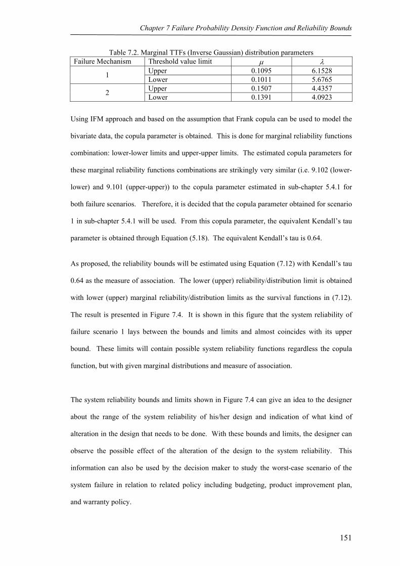
Chapter 7 Failure Probability Density Function and Reliability Bounds
Table 7.2. Marginal TTFs (Inverse Gaussian) distribution parameters Failure Mechanism Threshold value limit μ λ
Upper 0.1095 6.1528 1 Lower 0.1011 5.6765 Upper 0.1507 4.4357 2 Lower 0.1391 4.0923
Using IFM approach and based on the assumption that Frank copula can be used to model the
bivariate data, the copula parameter is obtained. This is done for marginal reliability functions
combination: lower-lower limits and upper-upper limits. The estimated copula parameters for
these marginal reliability functions combinations are strikingly very similar (i.e. 9.102 (lower-
lower) and 9.101 (upper-upper)) to the copula parameter estimated in sub-chapter 5.4.1 for
both failure scenarios. Therefore, it is decided that the copula parameter obtained for scenario
1 in sub-chapter 5.4.1 will be used. From this copula parameter, the equivalent Kendall’s tau
parameter is obtained through Equation (5.18). The equivalent Kendall’s tau is 0.64.
As proposed, the reliability bounds will be estimated using Equation (7.12) with Kendall’s tau
0.64 as the measure of association. The lower (upper) reliability/distribution limit is obtained
with lower (upper) marginal reliability/distribution limits as the survival functions in (7.12).
The result is presented in Figure 7.4. It is shown in this figure that the system reliability of
failure scenario 1 lays between the bounds and limits and almost coincides with its upper
bound. These limits will contain possible system reliability functions regardless the copula
function, but with given marginal distributions and measure of association.
The system reliability bounds and limits shown in Figure 7.4 can give an idea to the designer
about the range of the system reliability of his/her design and indication of what kind of
alteration in the design that needs to be done. With these bounds and limits, the designer can
observe the possible effect of the alteration of the design to the system reliability. This
information can also be used by the decision maker to study the worst-case scenario of the
system failure in relation to related policy including budgeting, product improvement plan,
and warranty policy.
151

Chapter 7 Failure Probability Density Function and Reliability Bounds
Marginal Reliability
0
0.2
0.4
0.6
0.8
1
0.05 0.1 0.15 0.2 0.25 0.3Million cycles
Rel
iabi
lity
Lower Limit - 1Upper Limit - 1Reliability PC 1Lower Limit - 2Upper Limit - 2Reliability PC 2
Figure 7.3 Marginal reliability functions and reliability limits of the bivariate degradation data
(bivariate CSDT Model 1)
Reliability Bounds and Limits - scenario 1
0
0.2
0.4
0.6
0.8
1
0.05 0.075 0.1 0.125 0.15 0.175Million cycles
Rel
iabi
lity
System reliabilityUpper boundLower boundUpper limitLower limit
Figure 7.4. System reliability bounds and limits for fatigue-crack data Model 1 failure scenario 1
7.6. Discussion on System PDF Adjustment and Bivariate System Reliability
Bounds and Limits
It was shown that when a system has k failure mechanisms then the TTF joint distribution
function will be a surface with k+1 dimension. Since a joint PDF should integrate to 1 and
only part of joint probability density function with the same marginal TTF input is needed
(e.g. the diagonal section of (bivariate) PDF as shown in Figure 7.1), its integration will not
152
Chapter 7 Failure Probability Density Function and Reliability Bounds
equate to 1. Therefore, in order to get the correct system PDF value, normalization should be
performed.
This normalization is also important for bivariate and multivariate PDF obtained using the
proposed Models 2 and 3 because the marginal and system PDF are not obtained directly using
predicted TTF data. Instead, they are obtained as a function of the marginal and system PDF
of the PCs. Therefore, for these two models, the normalization should be performed not only
to the system TTF PDF but also to the marginal TTF PDF. This will result in the adjusted
marginal and system TTF PDF which can be used for further analysis.
There is another interesting aspect of the system distribution function. As shown in Figure
7.1, the system distribution function, for bivariate degradation system, that is needed is the
diagonal section only. However, by looking at Figure 7.1, where the values of system PDF
with all possible combinations of marginal TTF data, additional information of the system can
be obtained. It was shown in this figure that the peak of the system PDF tends to be closer to
the 1st failure mechanism. This can be interpreted that the 1st failure mechanism has slightly
higher severity than the 2nd failure mechanism. With this additional information, the designer
can have additional illustrative idea about the possible improvement needed for the system and
how it should be redesigned, if necessary. Moreover, since this information can be presented
in the forms of both numerical and graphical, it will be more informative for the decision
maker to understand the information and to decide further steps/analysis needed.
In the second part of the discussion of this chapter, bounds for the system reliability function
are obtained. These are obtained with assumptions that the marginal distribution functions are
known and with additional information of the measure of association. The information of the
measure of association is used to improve the reliability bounds. These are needed as part of
the uncertainty analysis of the system. This information gives both the designer and decision
maker input for further system improvement consideration and risk analysis.
153

Chapter 7 Failure Probability Density Function and Reliability Bounds
For further uncertainty/risk analysis, the possible variability of the threshold value of each
failure mechanism of the system can also be included in the reliability analysis. The inclusion
of threshold values variability will provide the reliability limits. Combining this analysis with
reliability bounds improvement given measure of association, will present combined improved
reliability limits. These limits will provide information of the effect of the uncertainty or
variability of actual decision of threshold value (at the time of failure) to the possible system
reliability given the available data and without copula function assumption. In order to get the
lower (upper) reliability limit, use the lower (upper) marginal reliability limits (w.r.t the lower
(upper) threshold value limits) as the inputs of Equation (7.12) or (7.13). These limits can be
used for further system analysis and uncertainty/risk analysis. As mentioned, there is possible
subjective expert opinions on the failure definition and subjective interests on the system.
These subjectivities can matter hugely depends on the impact from the failure behaviour of the
system. Therefore, this information can be used to get objective ideas of the system
characteristics and is useful not only for the system designer (i.e. in modifying the design of
the system) but also for the decision maker in the organization.
The adjusted system PDF for the combination of lower-lower and upper-upper threshold
values limits can also be obtained. These adjusted system PDF w.r.t. the combined improved
reliability bounds will help the designer to understand the effect of the design to the system
failure characteristics better and also to help the designer to plan the design improvement
according to the purposes of the system. As for the decision maker, this information will be an
input for risk analysis and for finding the optimal decision. The adjusted system PDFs related
to the reliability bounds are presented in Figure 7.5.
It can be seen in Figure 7.5 that the system PDF related to the lower (upper) reliability bound
has higher (lower) peak than the estimated system PDF. The system PDF related to the
reliability bounds gives an illustration of the range of the failure probability and what to expect
154
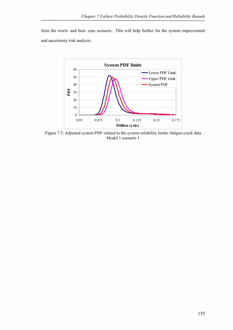
Chapter 7 Failure Probability Density Function and Reliability Bounds
from the worst- and best- case scenario. This will help further for the system improvement
and uncertainty/risk analysis.
System PDF limits
0
10
20
30
40
50
60
0.05 0.075 0.1 0.125 0.15 0.175Million cycles
Lower PDF LimitUpper PDF LimitSystem PDF
Figure 7.5. Adjusted system PDF related to the system reliability limits: fatigue-crack data
Model 1 scenario 1
155


Chapter Eight
Bivariate Constant Stress Accelerated Degradation Test
Degradation testing has been used as an alternative of life time testing especially when no failure
occurs during the test. However, with the combination of higher quality and reliability of
products and the limited time period between design and release time, even degradation test under
normal use stress level might not provide sufficient data for evaluation of product’s life
characteristics (Nelson, 2005). Therefore, motivated by the idea of accelerated life testing (ALT),
a type of degradation testing namely accelerated degradation testing (ADT) has been developed.
Similar to ALT, there are several strategies of ADT categorized by the application of the stress
levels during the test, namely:
1. Constant-stress ADT (CSADT)
2. Step-stress ADT (SSADT)
3. Progressive-stress ADT (PSADT)
In CSADT, there are usually two or more groups of samples. Each group of samples is tested
under certain stress level which is different from stress levels applied in other test groups. The
157

Chapter 8 Bivariate Constant Stress Accelerated Degradation Test
stress can be temperature, humidity, or other type of stresses depends on what drives the failure
mechanism(s). The stresses applied are usually higher then the use stress level to accelerate the
degradation process. Therefore, extrapolation model may be needed in order to evaluate the
product’s life characteristics under use stress level. Some results of the works in this area can be
found for examples in the reports of Chang (1993), Boulanger and Escobar (1994), Meeker et.al
(1998), Yang (2002), and Bae and Kvam (2004). The focus of these works is on deterministic
CSADT. A non-parametric CSADT study can be found, for example, in Shiau and Lin (1999). In
addition, literatures on CSADT plan include for examples Park and Yum (1998), Yu and Chiao
(2002) and Yu (2003).
Similar to constant-stress ALT (CSALT), CSADT also needs more samples than the other
accelerated plans because for each stress level a group of random samples is needed. To reduce
the experimental cost and difficulty in providing the required number of samples and test
equipments, PSADT and SSADT strategies can be implemented. In both strategies, the stress
level is altered over time. In PSADT, the stress is altered progressively over time whereas in
SSADT the stress is altered after certain period of time. Because of the higher difficulty and
complexity in degradation modelling, only few works in SSADT area can be found currently
compared to its counterpart in life testing. These few works in SSADT can be found for examples
in Chang et.al (1999), Tseng and Wen (2000), Tang et.al (2004), and Park et.al (2004).
Meanwhile, PSADT can be regarded not yet explored.
The ADT works that have been mentioned focus in univariate degradation test. However, as
mentioned in previous chapters, it is not unusual to find more than one function or failure
mechanism in a modern product because of the increase of product complexity. In this case, a
model that can accommodate multiple performance characteristic (PC) in an ADT plan is needed.
In relation to constraints such as costs, availability of samples and test equipment, time/project
limitation, SSADT may be preferred. However, the testing procedure is more complex. The
158

Chapter 8 Bivariate Constant Stress Accelerated Degradation Test
changing of the stress levels needs to be done carefully in order not to change the failure
mechanisms. Moreover, there may be difficulty in the operation of test equipments. The
availability of suitable model and analysis method for bivariate/multivariate degraded system is
also the concern in executing this test plan.
Considering these difficulties, bivariate CSADT models will be proposed in this chapter because
it can be regarded as the basis for multivariate CSADT model and analysis. Besides, the test
procedure and assumptions needed is simpler than SSADT or PSADT. Furthermore, even though
the complexity of products is increasing, it is not expected that the products become too complex
with too many failure mechanisms. Therefore bivariate CSADT modelling will provide a good
starting point in exploring an alternative degradation test model and multivariate ADT model.
The main assumptions of the bivariate CSADT model are:
1. There are two main failure mechanisms, each with its irreversible PC degradation that can be
observed and monitored,
2. The data gathered from constant-stress degradation test (CSDT) is not sufficient for
evaluating the product’s life characteristics. Therefore, an ADT is needed,
3. There is only one acceleration stress factor,
4. The failure mechanisms initiated by the different stress levels are the same (i.e. the change of
stress level does not initiate different failure modes),
5. The number of samples and the measurement times for each stress level are predetermined,
6. The characteristics’ degradation observations or the transformed characteristics of marginal
data can be modelled using GLM,
7. CSADT is suitable for accelerated test strategy since it is easier to control the stress levels and
there will be no concern related to the effect of changing the stress levels during the test.
The discussion in will be started by the life-stress relationships which are the basic principles in
CSALT. This will be propagated to CSADT and will be the motivation of the discussion of the
159

Chapter 8 Bivariate Constant Stress Accelerated Degradation Test
relationships between certain factor of degradation data and stress in CSADT in the next sub-
chapter. After that, bivariate CSADT models will be proposed based on the principles discussed
in sub-chapter 8.2 and proposed bivariate CSDT models in chapter five. A numerical example
will be presented in chapter eight based on the actual experiment result.
The discussion in this chapter will display initial efforts of modelling bivariate CSADT and
provide additional information on the possible future research in degradation models. This might
give an idea on what modification or improvement that can be done on the current degradation
models. Therefore, since this chapter will discuss exploration of bivariate CSADT modelling, no
CSADT plans will be discussed. Nevertheless, with the increasing need and implementation of
ADT, ADT plan remain as necessary topic to be discussed in the future despites its complexity.
8.1. Basic Principles of Constant-Stress Accelerated Life Test
In this sub-chapter, principle related to CSALT will be discussed because its test procedure has
similarity to CSADT. In many CSALT models, the data is usually analyzed based on the simple
relationship between life (e.g. TTF) and an accelerating stress variable (Nelson, 2005). Therefore,
it is important to understand life-stress relationships. There are some life-stress relationships that
have been proposed and used in ALT which include Arrhenius and inverse power as special cases.
Summary of the widely used life-stress models are presented in Nelson (1990). The motivations
between life-stress relationships are the fact that many products are operated at relatively constant
stress environment and the availability of the TTF data from ALT.
Arrhenius relationship has been used widely to model relationships of product’s life and the stress
in the form of temperature. Meanwhile, inverse power relationship has been applied to model
relationships of product’s life and an accelerating stress in area of for examples electrical
insulations, light bulb filaments, and simple metal fatigue. These simple relationships usually can
160

Chapter 8 Bivariate Constant Stress Accelerated Degradation Test
be generalized into a linear model which relate the life characteristic (or its function) and the
stress (or its function). In general, a linearized life-stress relationship can be written as:
( )sh θ1− = A + B.l(s) (8.1)
where, is inverse of some life characteristics (θs) or “nominal life” for example ln(TTF)
or the nominal life while l(s) can be the transformation of the stress level for example ln(s) or 1/s
or other functions. The parameters A and B can be estimated from the ALT data and then are
used to estimate the product’s life at certain stress level.
( )sh θ1−
When planning for an ALT, (8.1) is usually combined with the life distribution information which
contains the characteristics of the spread of the TTF. For each stress level, a distribution density
function of the product’s life is obtained. It is usually assumed that the product’s life follows a
certain distribution function even though it is operated under different stress(es) levels. It means
that the distribution parameters values may be different at different stress levels while the
distribution functions are the same. This is true as long as different levels of the stress(es) during
the test do not trigger different failure mechanism.
In the combined life-stress relationships with the life distribution function, the “life” of the
product may refer to the specific life characteristic of the product such as mean, median or a
distribution percentile of the product’s life. In this case θs in Equation (8.1) may be replaced by a
function of the distribution parameter which may have a related life characteristic interpretation.
Combining distribution function approximation with simple life-stress relationships provides
more refined model than simple life-stress relationship of single unit sample. Exponential, log-
normal, and Weibull distributions are parametric distributions that are commonly used to describe
product’s life distribution together with life-stress relationships model. In combining the life
distribution and life-stress relationships models, certain additional assumptions may be needed.
The rest of the procedure remains the same.
161

Chapter 8 Bivariate Constant Stress Accelerated Degradation Test
As indicated, the use of combination between parametric life distribution and life-stress
relationships to model accelerated test needs TTF data. Unfortunately, in ADT, individual sample
TTF data may not be predicted at all except when Model 1 is applied. Therefore, alternative
definition of relationships between different stress levels is needed. This will be discussed in the
next sub-chapter.
Other model that is used to describe the effect of certain factors to lifetime of a system is
proportional hazard model. It is often used in survival analysis in biomedical field. In this model
the hazard rate of a system at a stress” level is a function of (or proportional to) its baseline
hazard. This might be utilized to develop alternative CSADT models. However, it will not be
explored since the models in this thesis need specific degradation or life distribution assumptions.
More information of this model can be found in Cox and Oakes (1984).
8.2. Basic Principles of Constant-Stress Accelerated Degradation Test
When the available TTF data is not sufficient, the knowledge obtained from established studies on
life-stress relationships may not be very useful, especially when bivariate CSDT Models 2 and 3
are used as the basic models. In the few references of ADT, the relationships between certain
factors of the degradation data and the stress level are usually unique to the applications (Nelson,
2005). These can be motivated by the known physical/chemical process, possible degradation
rate-stress relationships, or possible PC distribution parameter degradation rate-stress
relationships. In this chapter, the physical/chemical related degradation process will not be
discussed. We will instead focus on the degradation rate (or certain factor of degradation data)-
stress relationships with assumptions that the degradation data can be modelled as in chapter five.
The general assumptions of these relationships model that will be used in this chapter can be
presented as follows:
162

Chapter 8 Bivariate Constant Stress Accelerated Degradation Test
1. Each marginal PC follows a marginal parametric distribution function and its degradation data
at a stress level can be modelled using bivariate degradation Model 2 or 3,
2. The degradation rate of certain factor(s) of marginal degradation data can be modelled as a
function of the stress level,
3. The marginal PC or its certain marginal distribution parameter (or their function) can be
presented as a simple linear function of time.
Assume that the expected value of the PC or marginal distribution parameter (or their function)
can be modelled as simple linear function of time. For each stress level, the degradation rate
component is assumed constant over time but different from one stress level to the other stress
levels. In general, the degradation rate can be written as follows,
β2 = f(s) (8.2)
where β2 is the degradation rate while f(s) is a function of the stress. These proposed relationships
are discussed as follows.
Marginal Performance Characteristic degradation rate-stress relationships
Assume that the expected value of the (possibly transformed) marginal PC can be expressed as,
E(f-1(Yi)) = Xi.β = β1 + β2.ti (8.3)
The parameter β2 is the degradation rate of the marginal PC. It is a function of the stress level as
in the (8.2). The definition of f(s) depends on the acceleration variable and the most suitable
relationship. If for example the acceleration variable is temperature, Arrhenius rate relationship
may be the suitable to represent the degradation rate. In this case, Equation (8.2) may be written
as,
β2 = β2a. exp(-γ/T), (8.4)
163

Chapter 8 Bivariate Constant Stress Accelerated Degradation Test
where T = absolute temperature in Kelvin. When the acceleration variable is voltage, power
function can be used instead as the degradation rate. As other alternative, Equation (8.1) can also
be used to describe relationships between β2 and stress level with the left hand side of Equation
(8.1) becomes 12( )h− β . The unknown parameters in Equations (8.2) and (8.3) are estimated
from the marginal ADT data.
Examples of the use of Arrhenius model to describe the relationship between degradation rate and
stress level can be found in Meeker et.al. (1998), Escobar et.al. (2003) while Chang (1993) used
generalized Eyring to describe the acceleration factor.
Marginal degradation distribution parameter degradation rate-stress relationships
If the bivariate CSADT model is based on the idea of bivariate CSDT Model 2, relationships
between the degradation rate of the marginal degradation distribution parameter regression
function and stress are needed. The form is similar to (8.3) excepts that the left hand side of the
equation is E(f-1(U)) which contains the expected values of (possibly transformed) marginal
degradation distribution parameters.
An extra attention has to be given to this relationship model because there may be more than one
distribution parameter for each marginal PC. Since not all distribution parameters are functions of
time, different treatments are needed. For the distribution parameter which is a function of time,
the degradation rate of the function can be modelled as a function of the stress level. On the
contrary, a distribution parameter which is not a function of time may or may not be a function of
the stress level. Some examples of the relationships between the distribution parameter and stress
will be presented here.
164

Chapter 8 Bivariate Constant Stress Accelerated Degradation Test
Simple Normal distribution parameter–stress relationships
If the marginal PC can be modelled using Normal distribution, there are two distribution
parameters for each PC at each measurement time, namely μ (mean) and σ (standard deviation).
Let assume:
1. The standard deviation σ is constant over time for each stress level,
2. The standard deviation σ may or may not be a function of the stress level. If σ is a function of
the stress level, then the relationships between σ and the stress level can be written as,
σ(s) = β3(s) (8.5)
3. The mean of the marginal degradation data μ or its function of each stress level depends on
time. Therefore, GLM-PA approach will be used to do the regression of μ at each stress level
and μ can be expressed as:
( )( ) tstf ., 21
1 ββμ +=− (8.6)
Where s is the stress level and t is measurement time
4. The degradation rate of ( )( )1 ,f t s− μ is a function of the stress level. That is )(2 sf=β as
in the Equation (8.2). The stress level in this function can be in the form of the original value
or its transformation such as the log or the inverse of the stress.
If the standard deviation σ is assumed independent of time, an average of all σ values taken during
the degradation observations can be used as an estimate. This parameter represents the spread of
degradation observations taken at certain stress level. For certain application, modelling σ as a
function of time may be needed. To use this assumption, further study and more knowledge on
test data are needed.
165

Chapter 8 Bivariate Constant Stress Accelerated Degradation Test
Simple Weibull distribution parameter degradation rate-stress relationships
When the marginal degradation distribution follows Weibull distribution, the shape parameter (β)
may be assumed to be independent of stress level but dependent of time or dependent of both
factors, while the scale parameter (α) is dependent of both time and stress level. The shape and
scale parameters are assumed independent of each other. Therefore, the assumptions can be
concluded as follows:
1. The shape parameter (β) is a function of time, that is:
( )( ) ttf .21
1 βββ +=− (8.7)
If β is independent of stress level, then β2 is a constant. On the other hand, if β is dependent
of both stress level and time, then β2 is modelled using Equation (8.2),
2. The scale parameter (α) at a stress level is a function of time, that is:
( )( ) tstf ., 21
1 ββα +=− (8.8)
As in the other equation, transformation of the stress and/or time may be needed in order to be
able to use simple linear function. And since β2 is related to the stress level, it can be represented
by Equation (8.2).
Further consideration of the degradation distribution degradation rate-stress
relationships
The judgment to model marginal degradation distribution parameters with independency or
dependency of measurement times and/or stress level depends on some concerns and available
knowledge. In ALT, there are more studies and experiences in this subject. In ALT, the standard
deviation of the life-time distribution is usually assumed independent of the stress level especially
because it is easy to use and because of previous experiences in certain products which suggest
the adequacy of constant spread of life distribution over all stress levels (Nelson, 1990).
However, some products indicate the existence of spread of life distribution as a function of stress
166

Chapter 8 Bivariate Constant Stress Accelerated Degradation Test
level. For example, some electrical insulations test data shows smaller spread of life distribution
at lower stress level compared to higher stress level. Unfortunately, in certain distribution
function, the use of life-time distribution's spread dependent of stress levels may produce crossing
points between probability plots of life at low and high stress levels. This will produce inaccurate
evaluation around the crossing point.
Meanwhile, there is no sufficient research has been carried out yet in the PC degradation-stress
relationships. However, since they show a good prospect for evaluating life characteristics from
bivariate CSADT data, further study may be valuable to perform. Therefore, more references to
the actual experiment data are needed to conduct further study on this subject. This study is
needed for the bivariate CSADT Models 2 and 3. When ADT model with random-coefficient is
used as presented in Nelson (1990), further development is needed to incorporate this simple
model with bivariate CSADT Model 1. However, since in bivariate CSADT Model 1 the system
reliability is estimated from the predicted TTF, life-stress relationships model will be applied
instead of relationships model between certain parameter of the degradation data and stress levels.
8.3. Bivariate CSADT Model
Three bivariate CSADT models will be discussed in this sub-chapter. These models are the
extension of the models presented in chapter five.
8.3.1. Bivariate CSADT Model 1
This model is based on the bivariate CSDT Model 1 presented in chapter five. The assumptions
of its CSDT counterpart are also valid for this model with the following additional assumptions,
1. Each marginal PC is tested according to CSADT procedure and might be tested separately to
other marginal PC. However, the acceleration variable and the stress levels are assumed the
same for both PCs,
167

Chapter 8 Bivariate Constant Stress Accelerated Degradation Test
2. The degradation data of each marginal PC tested under a stress level is analyzed according to
stage 1 of bivariate CSDT Model 1 to obtain the predicted TTFs. Therefore, if for example
each marginal PC is tested under three stress levels (which should be the same for all PCs),
six sets of predicted TTF data are obtained from the bivariate degraded system,
3. The predicted marginal TTF distribution function of a marginal PC is the same for all stress
levels but the parameters values can be different,
4. For each marginal PC, certain life-stress relationship is applicable and the predicted TTF
distribution parameters at the use/operational stress level can be estimated from this
relationship,
5. Dependency between PCs may be a function of the stress level but not of time.
The bivariate CSADT Model 1 consists of three stages. These stages are:
1. Stage 1: Perform the bivariate CSDT Model 1 – stage 1 to every set of marginal degradation
data of each marginal PC and each stress level. Obtain the predicted marginal TTFs and
analyze the possible TTF distribution functions. Note that for a PC, the TTF data of all stress
levels follows the same distribution function,
2. Stage 2: Based on the life-stress relationships combined with the assumed TTF distribution
function obtained from stage 1, calculate the marginal TTF distribution parameters at
operational stress level. This can be done by estimating the unknown parameters of Equation
(8.1) with the left hand side of the Equation (8.1) replaced by a (possibly a function of) TTF
distribution parameter instead of the TTF data. The estimation can be done using MLE
procedure,
3. Stage 3: Assume that the copula function is known and valid for all stress levels. If it is
assumed that the copula parameter is a function of stress level, define this relationship and
incorporate this in the IFM procedure. Perform IFM for all stress level simultaneously.
Otherwise, perform IFM for each stress level separately and use the average of the copula
parameter w.r.t the stress level as estimation. Then use it together with the estimated
168

Chapter 8 Bivariate Constant Stress Accelerated Degradation Test
marginal TTF distribution parameters at the use stress level to obtain the system reliability
using the similar procedure as in the bivariate CSDT Model 1 – stage 2.
The procedure of the stage 1 of this model is clear since it is basically the same as the procedure
of bivariate CSDT Model 1 – stage 1. Therefore, no additional discussion will be presented.
Stage 2 is basically the same as performing CSALT analysis to the predicted marginal TTF data
of each PC. If, for example, the predicted TTF distribution function of a PC can be represented
by Inverse Gaussian distribution, then there are two distribution parameters at each stress level,
i.e. μ (mean) and λ (shape parameter). Assume that the shape parameter (λ) is not a function of
stress level (s). Therefore, the average of the shape parameter (λ) will be used for the use stress
level. On the contrary, the mean (μ) is a function of stress level. Therefore, the relationship
between the mean and the stress level can be presented as follows,
( )1(h s− μ )
)
= A + B.l(s) (8.9)
where is the inverse of the mean or its function at stress level s. The unknown
parameter A and B can then be estimated and used to find the mean parameter at the use stress
level.
( )1(h s− μ
With this information, we can proceed to stage 3. With the assumption that the copula function is
known and valid at all stress levels, perform IFM to the predicted data at each stress level. This is
executed by maximizing Equation (5.21) w.r.t. copula parameter. If the copula parameter is a
function of stress level, include the relationships model of the copula parameter in the IFM.
Therefore, the unknown parameter of the model can be estimated and copula parameter estimation
at certain stress level can be obtained. Afterward, the system reliability can be calculated using
Equations (5.16) or (5.17) as in the chapter five.
169

Chapter 8 Bivariate Constant Stress Accelerated Degradation Test
8.3.2. Bivariate CSADT Model 2
This model is motivated by bivariate CSDT Model 2. Therefore, the degradation distribution
parameter data is needed because the modelling is performed on this type of data. The additional
assumptions needed for this model are,
1. Each PC is tested according to CSADT procedure and might be tested separately. However,
the acceleration variable and the stress levels are assumed the same for both PCs,
2. For every marginal PC, at least one of the marginal degradation distribution parameter is a
function of the stress level and their relationships can be defined as discussed in the sub-
chapter 8.2,
3. The marginal degradation distribution parameters can be modelled using GLM-PA with
simple linear function,
4. The measurement times at a stress level should be the same for both PCs but could be
different for different stress level,
5. The between PCs dependency may be a function of the stress level but not of time.
This model consists of three stages, which are basically: modelling and analysis of the marginal
degradation data, analysis of the copula parameter, and system reliability estimation. They can be
presented as:
1. Stage 1: Perform the procedure of bivariate CSDT Model 2 – stage 1 on each PC at all stress
levels to obtain the "degradation" path of the marginal PC distribution parameter. Include the
relationships definition between the slope of the marginal PC distribution parameter
"degradation" path and the stress level and estimate the unknown parameters numerically,
2. Stage 2: Assume that the copula function is known and valid for all stress levels. If the
copula parameter is a function of stress level, include this relationship in the model and
perform IFM to the log-likelihood function simultaneously to obtain the unknown parameters,
3. Stage 3: Use the information obtained in the previous stages to estimate the parameters at the
concern stress level and system reliability as in the stage 2 of bivariate CSDT Model 2.
170

Chapter 8 Bivariate Constant Stress Accelerated Degradation Test
The first stage of this model is similar to the first stage of bivariate CSDT Model 2. However, the
first and third steps of the iterative re-weighted estimation procedure to estimate β are different
than the steps used at bivariate CSDT Model 2 because β in this CSADT model is estimated
numerically instead of using ordinary least squares (OLS) or iteratively re-weighted least squares.
This is caused by the inclusion of the relationship model between the degradation rate of the
marginal distribution parameter and stress level. The rest of the procedure is the same as in the
CSDT model. The estimated regression parameters obtained in stage 1 will be used in stage 2.
Before estimating the system reliability at stage 3, the copula parameter is needed. It is obtained
using IFM approach and assumption that the copula parameter may or may not be a function of
stress level. Since the marginal PC distribution parameters for each stress level have been
obtained in stage 1, the copula parameter at each stress level can be estimated by maximizing the
following equation (which has appeared also as Equation (5.33)) w.r.t copula parameter,
( )( ) ( )( )( )1 2(1) (2)
1
ˆ ˆln ,m
ij ij ij iji
c F Y t F Y t=∑ (8.10)
Using Equation (8.10) the copula parameter at each measurement times at a stress level can be
obtained. The mean of these estimations is the copula parameter for that stress level. If the
copula parameter is a simple linear function of the stress level, these copula parameter estimations
can be used to estimate the unknown parameters of the function and predict the copula parameter
at certain stress level. Then, with the estimated marginal PC distribution parameters
"degradation" path at use stress level, the system reliability can be estimated/predicted based on
the following equation,
R(t) = P[Yt(1) < c(1)⏐t, Yt
(2) < c(2)⏐t] = C{F(1)(y(1)|t), F(2)(y(2)|t)} (8.11)
171

Chapter 8 Bivariate Constant Stress Accelerated Degradation Test
8.3.3. Bivariate CSADT Model 3
This model is motivated by bivariate CSDT Model 3. As in the previous models, the assumptions
of its CSDT model counterpart are also valid except that the copula parameter is assumed to be
not a function of time. And as the other CSADT models, additional assumptions are needed and
they are,
1. Each PC is tested according to CSADT procedure and might be tested separately. However,
the acceleration variable and the stress levels are assumed the same for both PC,
2. The degradation data of every PC can be modelled using GLM-PA with simple linear
function to represent the expected value of the degradation data (or its inverse function),
3. The relationships between the degradation rate and stress level can be presented as in the sub-
chapter 8.2. The estimation of the unknown parameters of this relationship can be used to
estimate the marginal degradation path at the use stress level,
4. The marginal degradation distribution parameters can be obtained from the regression
analysis of the marginal PC,
5. The measurement times at a stress level should be the same for both PCs but could be
different for different stress level,
6. The between PCs dependence is not a function of the time. Therefore, the average will be
used to estimate the copula parameter at a stress level.
This model also consists of three stages, which can be summarized as follows,
1. Stage 1: Perform the procedure of bivariate CSDT Model 3 – stage 1 on each PC for all stress
level simultaneously to obtain the degradation path of a marginal PC. In this stage, the
relationships definition between the degradation rate of the marginal PC and the stress level is
needed. OLS and iteratively re-weighted least squares will not be performed. Instead,
parameters β are estimated numerically as in bivariate CSADT Model 2 – stage 1. And as in
its CSDT model counterpart the marginal degradation distribution parameters should be able
to be estimated from the marginal degradation function,
172
Chapter 8 Bivariate Constant Stress Accelerated Degradation Test
2. Stage 2: Assume that the copula function is known and valid for all stress levels. Perform
IFM to every stress level to obtain copula parameter as in the bivariate CSDT Model 3. If the
copula parameter is a (simple linear) function of the stress level, use the IFM result to
estimate the unknown parameters of the function and estimate the copula parameter at
concern stress level. Otherwise, the average of the copula parameter w.r.t the stress level is
used as estimation.
3. Stage 3: Use the information obtained in stages 1 and 2, to estimate the system reliability at
the concern stress level.
The first stage is basically similar to the first stage of the bivariate CSDT Model 3. The
differences are the inclusion of the relationship model between the degradation rate and stress and
the use of numerical method to estimate β.
The dependency between PCs at every stress level can be estimated using IFM approach as in the
bivariate CSDT Model 3. This estimation is executed for all stress levels. When the copula
parameter is a function of stress level, the mean of the copula parameter at each stress level is
used to estimate the unknown parameters of the copula parameter function. The results are used
to estimate the copula parameter at certain stress level. This information is used together with the
result of stage 1 to evaluate the system reliability at the certain stress level based on the Equation
(8.11).
8.4. Discussion on Bivariate CSADT Models
Three bivariate CSADT models have been proposed. These models are the results of the effort to
explore the possibility of bivariate CSADT data modelling. They are natural extension of the
bivariate CSDT models presented in chapter five. There are some constraints w.r.t. the test
procedures and assumptions in order to implement these models. However, it has been shown
173

Chapter 8 Bivariate Constant Stress Accelerated Degradation Test
that it is possible to model bivariate degradation data from CSADT with between PCs dependence
assumption. However, further study is still needed to implement and improve the models
including relaxing some assumptions.
Firstly, the comparison between the three proposed models will be discussed. They are presented
in the following points:
1. Acceleration variables: In the three models, the stress factor which motivates the acceleration
is only one and the same for both PCs. This assumption may not be valid for all system, but it
is used here for simplicity. In the case when the PCs might have different stress factors or
combined stress factors further study is needed to determine if the performance characteristics
can be considered independent despites the same operational condition of the system, how to
conduct the CSADT, and how to develop the model,
2. Test stress levels: The stress levels of both performance characteristics, with assumption that
the performance characteristics have the same acceleration variable, are assumed the same for
all performance characteristics. This is needed to ensure that the copula parameter, which
reflects the between performance characteristics dependence, can be estimated from the
degradation data. In the three models, a copula parameter is obtained at each stress level.
This is the reason of the need of conducting the CSADT with same stress levels for both
performance characteristics. This is obviously one of the constraints of these CSADT
models. Additional research is needed to overcome this problem and problems appear when
the failure mechanisms are motivated by different stress factors or a combination of stress
factors,
3. Measurement times: As in the CSDT model, the measurement times of Model 1 do not have
to be the same for both PCs. However, for the other two CSADT models, this is needed since
the copula parameter at each stress level should be estimated from the degradation data at
certain measurement time. In this case, Model 1 is a bit more flexible that the other two
models. Notice that the measurement times of a PC at different stress levels do not have to be
174

Chapter 8 Bivariate Constant Stress Accelerated Degradation Test
the same, since copula parameter is evaluated at each stress level and not across the stress
levels,
4. Between PCs dependence: It should be noted that the copula parameter obtained by Model 1
reflects the dependence between the TTFs of the failure mechanisms while the one obtained
by Models 2 and 3 reflects the dependence between the PCs' degradation observations.
However, even though they have different dependence implications, they still represent the
dependence between the failure mechanisms but in different ways and are still valid to
estimate the system reliability,
5. Reliability estimation: In the bivariate CSADT Model 1, the marginal and system reliability
functions are estimated via the predicted TTF data. On the contrary, the other two models do
not predict the marginal TTF data of the samples but estimate the marginal and system
reliability through the degradation data analysis.
Secondly, following the above discussion, the possible improvements of the models will be
presented in the following points:
1. Further study w.r.t the relationships between the stress and degradation rate of PC(s) or
distribution parameter(s) of the marginal degradation data is needed in order to understand
how to model these better and to get the information at the use stress level which will be
needed to estimate the marginal and system reliability at certain condition. With good
understanding of these relationships, improvement to the CSADT model can be performed
and better estimation of the data at use stress level can be obtained,
2. For some systems, the marginal failure mechanisms may be triggered by different stress
factors (or different combination of stress factors) even though it is operated at the same
operational condition. In this case, further investigation is needed to determine whether the
failure mechanisms are independent or dependent to each other, how to model the
relationships between the failure mechanisms dependency and the stress variable(s) if any,
and the effect of the stress factor(s) to the system reliability,
175

Chapter 8 Bivariate Constant Stress Accelerated Degradation Test
3. Modelling of non-linear bivariate degradation path may need to be developed to provide an
alternative model. In order to do this, better understanding of the relationships between
stress(es) and certain characteristic(s) or parameter(s) of the marginal data as mentioned in
point (1) is important. The interpretation of the components of the model is also needed since
it may help the stake holders of the system to understand and improve the system closer to the
optimum target.
This discussion may give some illustration of the constraints and possible future improvements of
the proposed models. Despites all of these, the proposed models have served as exploratory
models that are able to model and analyze bivariate degraded system based on its bivariate
CSADT data. As shown in the examples of chapter five, analysis with independence and
dependence assumptions may result in different conclusions. That's why the alternative models
presented in this chapter will serve as additional options for CSADT model. They can also be
seen as a starting point to further development of the bivariate CSADT model. An example of the
implementation of these proposed models to the actual experiment data will be presented in the
next chapter.
176

Chapter Nine
Implementation of the Proposed Models to LED Test Data
Bivariate and multivariate CSDT models, bivariate CSADT models and reliability bounds and
limits for bivariate CSDT models have been proposed and discussed in the previous chapters.
The bivariate CSDT models have been implemented to fatigue-crack data from Bogdanoff and
Kozin (1985). However, this data is insufficient to demonstrate the other proposed models and
test conditions which are also discussed in this thesis. Therefore, a case study has been proposed
and tests were performed to collect the necessary data. In this case study, systems of light-
emitting diode (LED) lamps are studied. The reliability of the LED lamps arranged in a certain
system will be estimated and studied. In order to understand the product/system, a brief
introduction on the LED lamps will be given in the first sub-chapter. It will be followed by the
description of the design of the tests. The implementation of the proposed models performed on
the experiment data collected in the test will be presented in the third sub-chapter. This chapter
will be concluded by some discussion on the modelling and analysis results.
177

Chapter 9 Implementation of the Proposed Models to LED Test Data
9.1. LED Lamp
The publication on emission of light from semiconductor diode by H.J. Round in 1907 can be
seen as the beginning of the history of LED even though he was not the inventor of current LED
technology (Zheludev, 2007). Round (1907) reported in his publication what can be considered
as the first type of LED which was a Schottky diode. The second report that is regarded as the
early development of the LED technology is reflected in the work of O.V. Lossev which was
published in 1920s. Zheludev (2007) recognizes Lossev as the first person who realized the
potential of LED in telecommunication area. However, only at 1962 the first practical LED was
invented by Nick Holonyak, Jr. when he was working for General Electric. Compared to this first
practical LED, the current LED technology has been changing quite rapidly and it has been used
in many applications (such as: telecommunication instruments, traffic lights and signals,
architectural lighting, decorating related purposes, light source for machine vision systems, in
optical fibre and free space optics communications, etc.).
Currently, the potential of LED for general lighting source has also been explored. This is made
possible by the continuous development in LED technology through discovery in materials
science and extensive research and development. One of the important discoveries is the
invention of gallium nitride (GaN) LED in 1993 by Shuji Nakamura. Based on this invention, it
is now possible to produce white light using LED. The use of LED has also been predicted to be
able to save electrical power and fossil fuel. It is also more environmental friendly compared to
the current common lighting source energy (e.g. incandescent and fluorescent technology)
because of the reduction of hazardous materials used to produce it and it is also more efficient
(Schubert, 2003). Because of these reasons, there is extensive research on the implementation of
LED technology as lighting source which is also known as solid-state lighting (SSL). However,
since this technology is relatively new and there are different types of LED technology currently
available, the application and performance of LED lamps as general illumination source have also
significant differences. Therefore, it is important to study the performance characteristics (PCs)
178

Chapter 9 Implementation of the Proposed Models to LED Test Data
of the LED lamps in certain conditions (Narendran et.al., 2004). It will reveal the reliability of
the LED lamps and provides input for environmental, economical and policy considerations.
With the view to the potential of LED lamps as general illumination source and the rapid
development and changes in LED technology, study of the LED lamps reliability has drawn the
interest of many manufacturers who see the potential of future business in this area. LedNed BV
is one of the companies who sees the potential of LED lamps and has been actively developing
and delivering LED lamps since 2004. In order to have a good position in the market, LedNed
BV understands the need of research and development activities. That is why LedNed BV is also
interested in studying the reliability of different types lighting designs developed using different
types of LED. The information of the reliability of the LED lamps which are used in certain
usage arrangements will be useful for a company to assess the possibility of the success of the
product and other related issues. With LedNed BV supports, an LED lamps reliability case study
was conducted. The data collected from the experiment is used to study LED lamps arranged in
certain systems and tested in certain conditions which were discussed in the previous chapters.
The designs of the test and some general details of the lamps and the systems of the lamps are
presented in the following sub-chapter.
9.2. Test Design and Data Collection
As the case study of this thesis, two different types of LED lamps were observed. They were
tested in certain environmental conditions and the PCs of the lamps were recorded and used as the
data needed for the modelling and analysis.
Based on their literature review, Bürmen et.al. (2007) conclude that LEDs do not usually
experience catastrophic failure, but instead they will usually have degradation failures in the form
of degradation of the brightness and colour. However, in this thesis, the PC of the lamp that is
179

Chapter 9 Implementation of the Proposed Models to LED Test Data
observed is only the light output of the lamp which is measured in lux because of the
unavailability of the equipments to measure the colour change of the lamps. Degradation test is
used to assess the LED lamp reliability because LED, which is the main component of the LED
lamps, is known to have quite long life time compared to other lighting sources. The life time of
LED lamps is measured as the time when the light output of the lamps decreases until the first
time it passes certain value of the light output compared to the initial light output. This value is
also known as the critical value. There are different opinions of the life time of white LED lamps
which is also influenced by different LED technologies used and different critical value
definitions. In general, white LED lamps are assumed to have around 10,000 - 20,000 hours
(Bürmen et.al. (2007) and Bullough (2006)).
The first LED lamp type observed in this study is a high power white LED light bulb. This type
of lamp was tested only under the assumed operational condition i.e. at 25°C. The samples of
this type of lamp were burned continuously and the brightness level of the lamps was measured
using a lux meter. A total of 16 lamps were tested. They are labelled as A0, A1,…, A7, B0,
B1,…, B7. The lamps were set in a parallel setting and placed separately in a PVC cylinder. This
placement was designed to accommodate separate measurement of the lamps’ brightness without
disturbing other samples. Figure 9.1 shows the set up of this test.
Figure 9.1. High power white LED light bulb experiment set up
180

Chapter 9 Implementation of the Proposed Models to LED Test Data
This test was initially designed and performed by Martin Kools, a master student at Technology
Management Department (TU/e). Unfortunately, the measurement times were not well planned.
Nevertheless, the data can still be used to assess the reliability of the lamps with some noise.
However, since the data was not collected in the desired form, not all of the proposed models can
be used to analyze the data of the first type of LED lamp.
The second LED lamp type is LED tubular light. This lamp also produces white light but it is
built from low power LEDs. This lamp was tested for its light output under two different
environmental temperatures (i.e. 25°C and 55°C). These two temperatures were selected because
of the following reasons:
1. Alliance for Solid-State Illumination Systems and Technologies (ASSIST) recommendation
on the highest temperature for the test of low power LED component is 55°C (Bullough,
2006). This recommendation is made based on the possible junction temperature of the lamp
based on environmental temperature. This junction temperature is different and usually
higher than the ambient temperature and may lead to the possible maximum temperature at
which the LED and other components of the lamp can cease to operate,
2. The limited availability of samples. With respect to the number of available samples and the
plan to carry out not only CSDT but also CSADT, the test was performed at only two
different temperatures (i.e. two stress levels). This decision was made in view that the main
purposes of this experiment are to do preliminary reliability assessment of the lamps and as
implementation example of the proposed degradation models,
3. The availability of the temperature chambers. Initially there were two temperature chambers.
However, after validation test of the chambers, it turned out that only one chamber was
reliable. Therefore, parallel tests could not be performed. This means that the test would take
at least twice than the expected test time. Since there were other experiments in queue which
needed the temperature chamber, the degradation test were performed at two different
temperatures.
181

Chapter 9 Implementation of the Proposed Models to LED Test Data
Contrary to the LED light bulb test, the samples of the LED tubular light were not placed in a
separate container. This decision was made because of the size and shape of the LED tubular
light and the temperature chamber. To overcome the difficulty of placing the lamps, some boards
were built. At each board, 8 samples can be placed. The temperature chamber can hold
maximum two boards (see Figure 9.2). Since the lamps were not placed in separate container, a
device to measure the light output was also built. It consists of a dark box with a lux meter device
and a web-camera which are placed in the bottom-centre of the box. The lux meter reading can be
recorded via the web-camera. This arrangement is shown in Figures 9.3-9.5.
Figure 9.2. Placement of the LED tube lights inside the temperature chamber
Figure 9.3. Schema of the dark box for LED tubular light measurement (Kan, 2007)
At stress level 25°C, 16 lamps were tested. At pre-determined measurement times, the light
output of the lamps was recorded. The same was done to the samples tested at 55°C. However,
because of some unexpected catastrophic failures occured at stress level 55°C, only data from 14
samples at 55°C will be used in the bivariate degradation data analysis.
182
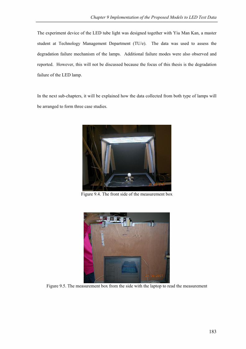
Chapter 9 Implementation of the Proposed Models to LED Test Data
The experiment device of the LED tube light was designed together with Yiu Man Kan, a master
student at Technology Management Department (TU/e). The data was used to assess the
degradation failure mechanism of the lamps. Additional failure modes were also observed and
reported. However, this will not be discussed because the focus of this thesis is the degradation
failure of the LED lamp.
In the next sub-chapters, it will be explained how the data collected from both type of lamps will
be arranged to form three case studies.
Figure 9.4. The front side of the measurement box
Figure 9.5. The measurement box from the side with the laptop to read the measurement
183
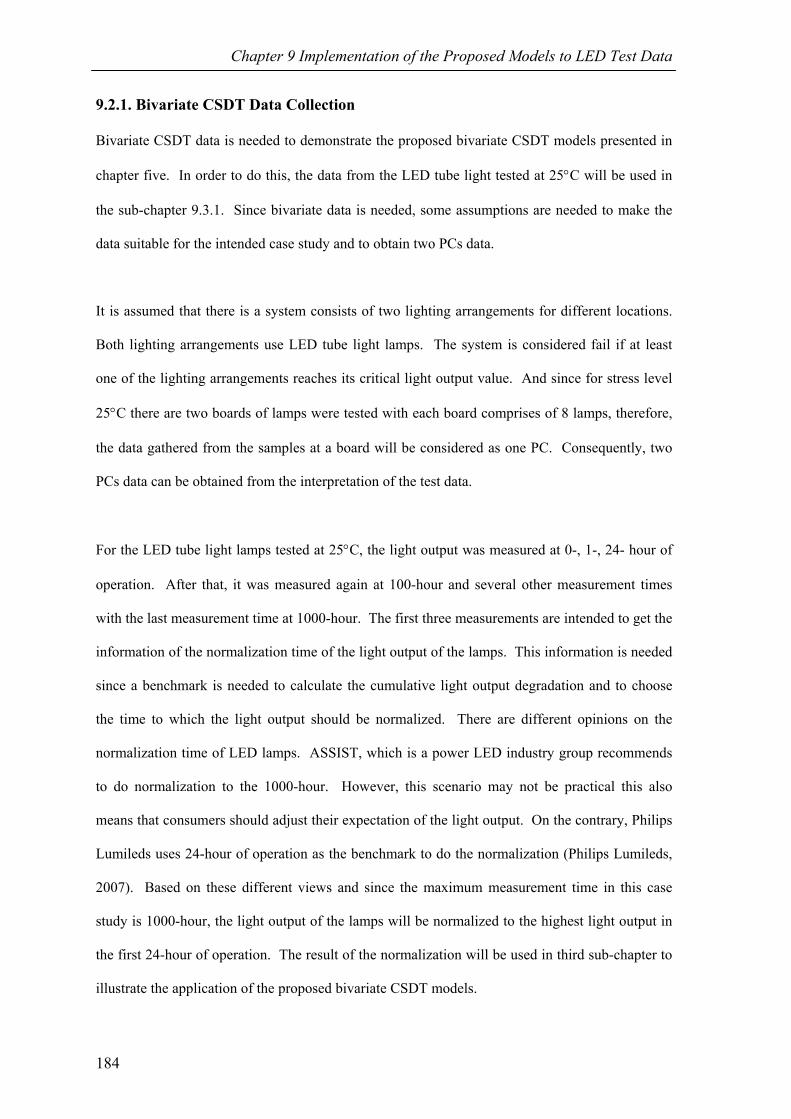
Chapter 9 Implementation of the Proposed Models to LED Test Data
9.2.1. Bivariate CSDT Data Collection
Bivariate CSDT data is needed to demonstrate the proposed bivariate CSDT models presented in
chapter five. In order to do this, the data from the LED tube light tested at 25°C will be used in
the sub-chapter 9.3.1. Since bivariate data is needed, some assumptions are needed to make the
data suitable for the intended case study and to obtain two PCs data.
It is assumed that there is a system consists of two lighting arrangements for different locations.
Both lighting arrangements use LED tube light lamps. The system is considered fail if at least
one of the lighting arrangements reaches its critical light output value. And since for stress level
25°C there are two boards of lamps were tested with each board comprises of 8 lamps, therefore,
the data gathered from the samples at a board will be considered as one PC. Consequently, two
PCs data can be obtained from the interpretation of the test data.
For the LED tube light lamps tested at 25°C, the light output was measured at 0-, 1-, 24- hour of
operation. After that, it was measured again at 100-hour and several other measurement times
with the last measurement time at 1000-hour. The first three measurements are intended to get the
information of the normalization time of the light output of the lamps. This information is needed
since a benchmark is needed to calculate the cumulative light output degradation and to choose
the time to which the light output should be normalized. There are different opinions on the
normalization time of LED lamps. ASSIST, which is a power LED industry group recommends
to do normalization to the 1000-hour. However, this scenario may not be practical this also
means that consumers should adjust their expectation of the light output. On the contrary, Philips
Lumileds uses 24-hour of operation as the benchmark to do the normalization (Philips Lumileds,
2007). Based on these different views and since the maximum measurement time in this case
study is 1000-hour, the light output of the lamps will be normalized to the highest light output in
the first 24-hour of operation. The result of the normalization will be used in third sub-chapter to
illustrate the application of the proposed bivariate CSDT models.
184

Chapter 9 Implementation of the Proposed Models to LED Test Data
9.2.2. Multivariate CSDT Data Collection
For the multivariate CSDT analysis, the data collected from the LED tube lights described in the
previous sub-chapter will be used as the first and second PCs. However, this is not enough to
demonstrate the implementation of the proposed multivariate models since more than two PCs are
needed. Therefore, the data collected from the high power LED light bulb will be considered as
the third and fourth PCs.
Recall that there were 16 high power LED light bulb samples tested at 25°C. The samples
labelled as B0, B1,..., B7 will be treated as the samples of the third PC while the samples labelled
as A0, A1,..., A7 will be treated as the samples of the fourth PC. It is assumed that there is a
lighting system consists of four lighting locations. Two of which use low power LED tube lights
and the rest use high power LED light bulbs.
Referring to the proposed multivariate CSDT models, unfortunately only Model 1 does not
require the same measurement time of all PCs. Therefore, the available data can only be used to
demonstrate implementation of this model. Nonetheless, the data can still be used to illustrate
reliability modelling and analysis of a system with multivariate degraded failure mechanisms.
The measurement times of the LED light bulb, unfortunately were not planned as carefully as the
LED tube lights experiment. Therefore more noise is expected from the data. However, this
problem sometimes cannot be avoided and therefore it is decided that the data will still be used in
the analysis. And since the LED light bulbs were not measured for 1- and 24- hour of operation,
the 0-hour light output measurement will be used as the benchmark for the normalization of the
light output.
185
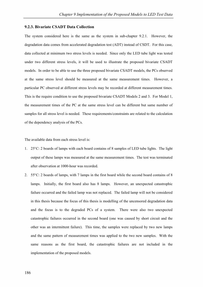
Chapter 9 Implementation of the Proposed Models to LED Test Data
9.2.3. Bivariate CSADT Data Collection
The system considered here is the same as the system in sub-chapter 9.2.1. However, the
degradation data comes from accelerated degradation test (ADT) instead of CSDT. For this case,
data collected at minimum two stress levels is needed. Since only the LED tube light was tested
under two different stress levels, it will be used to illustrate the proposed bivariate CSADT
models. In order to be able to use the three proposed bivariate CSADT models, the PCs observed
at the same stress level should be measured at the same measurement times. However, a
particular PC observed at different stress levels may be recorded at different measurement times.
This is the require condition to use the proposed bivariate CSADT Models 2 and 3. For Model 1,
the measurement times of the PC at the same stress level can be different but same number of
samples for all stress level is needed. These requirements/constraints are related to the calculation
of the dependency analysis of the PCs.
The available data from each stress level is:
1. 25°C: 2 boards of lamps with each board contains of 8 samples of LED tube lights. The light
output of these lamps was measured at the same measurement times. The test was terminated
after observation at 1000-hour was recorded.
2. 55°C: 2 boards of lamps, with 7 lamps in the first board while the second board contains of 8
lamps. Initially, the first board also has 8 lamps. However, an unexpected catastrophic
failure occurred and the failed lamp was not replaced. The failed lamp will not be considered
in this thesis because the focus of this thesis is modelling of the uncensored degradation data
and the focus is to the degraded PCs of a system. There were also two unexpected
catastrophic failures occurred in the second board (one was caused by short circuit and the
other was an intermittent failure). This time, the samples were replaced by two new lamps
and the same pattern of measurement times was applied to the two new samples. With the
same reasons as the first board, the catastrophic failures are not included in the
implementation of the proposed models.
186

Chapter 9 Implementation of the Proposed Models to LED Test Data
Based on the constraints and the availability of the data, for each PC at each stress level,
degradation data from 7 sample units will be considered. Therefore, one sample from each board,
which was tested under 25°C, will be randomly ignored. For the data collected at 55°C, only one
sample from the second board will not be included in the analysis. It will be assumed that we
only have 7 sample units for each PC tested at each stress level.
9.3. Modelling and Analysis
In this sub-chapter, three cases will be discussed. Detail of the cases will be given in the
respective sections. The related degradation data and the modelling and analysis of the data will
also be presented in the respective sections.
9.3.1. Bivariate CSDT Modelling and Analysis
The first case study is related to the proposed bivariate CSDT models. Consider a system that
consists of two lighting devices/arrangements. Both lighting devices are low power LED tube
lights. However, they may come from different population or follow different degradation
patterns because of the design of the system. In order to continue with the modelling and analysis
steps, some assumptions are needed.
The general assumptions applied to this system and the collected CSDT data are:
1. The lighting system consists of two sets of low power LED tube lights,
2. Each set of LED tube light has a degradation failure mechanism, which is the degradation of
the light output and it is considered as one PC of the system,
3. The system is considered fail if the light output (i.e. the PC) of at least one of the LED tube
light sets degrades to its critical light output value (which is pre-defined),
187

Chapter 9 Implementation of the Proposed Models to LED Test Data
4. Since the two sets of LED lights are assumed to be arranged as a lighting system which is
operated at certain environmental conditions (with ambient temperature of 25°C), it is
assumed that these LED light sets may not be independent of each other. Therefore,
dependence analysis is needed,
5. It is also assumed that CSDT test that has been performed can provide sufficient data needed
for the reliability assessment of the system.
With these information and assumptions, an effort to assess the reliability of the mentioned
system will be performed using the three proposed bivariate CSDT models. For each proposed
model, the assumptions related to the respective models as presented in chapter five are valid to
the respective models and the system in general.
In order to use the light output measurements to assess the system reliability, this observation
should be converted into cumulative degradation data (in percentage). Hence, normalization
needs to be performed. Consequently, it should be decided to which measurement time the
normalization is performed. After observing the experiment data, both PCs have their average
highest light output at 24-hour of operation. Therefore, it is used as the normalization benchmark
time. Based on this benchmark the cumulative degradation percentage can be calculated and
plotted. This data will be the input of the modelling and analysis steps. The cumulative
degradation data of both PCs is presented in Figure 9.6. It can be seen from Figure 9.6, that the
cumulative degradation curves of both PCs are relatively linear. Therefore, transformation of the
cumulative degradation data to linear form may not be needed.
188
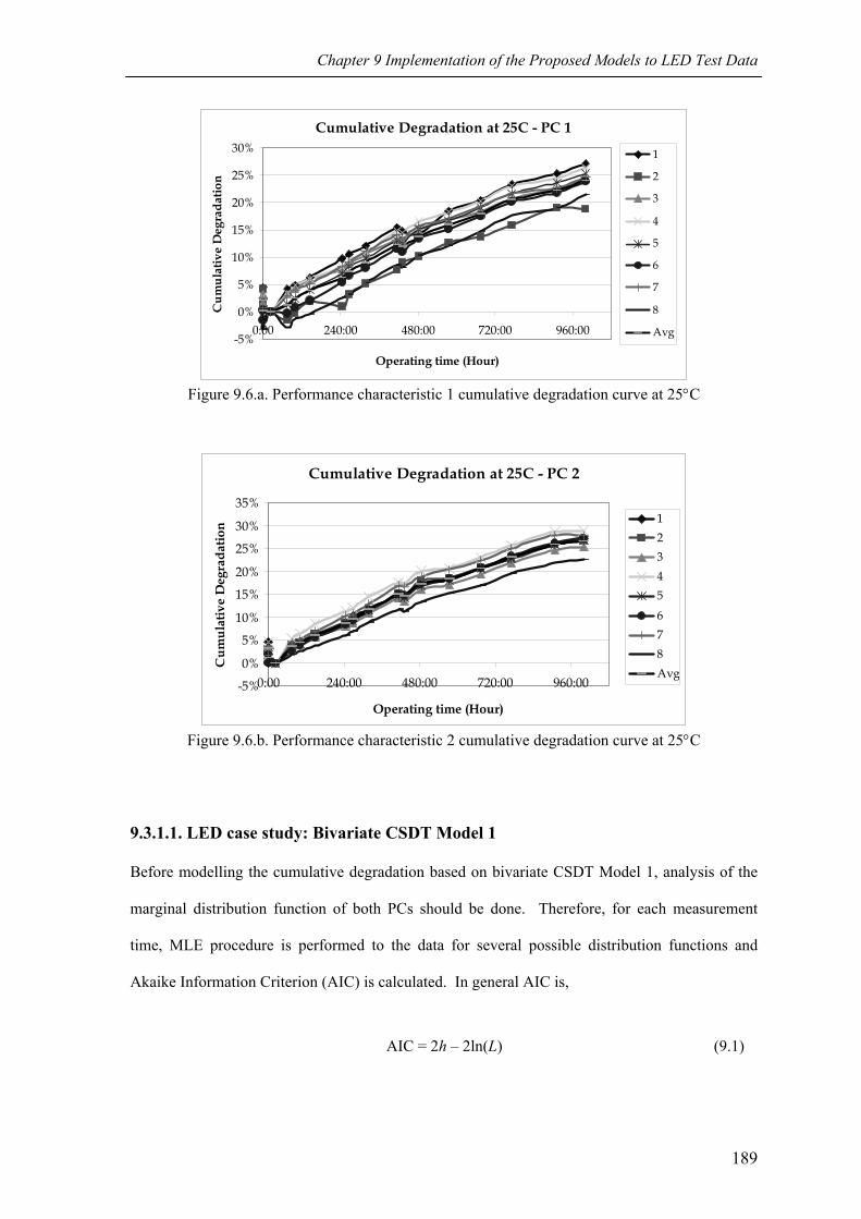
Chapter 9 Implementation of the Proposed Models to LED Test Data
Cumulative Degradation at 25C - PC 1
-5%
0%
5%
10%
15%
20%
25%
30%
0:00 240:00 480:00 720:00 960:00
Operating time (Hour)
Cum
ulat
ive
Deg
rada
tion
1
2
3
4
5
6
7
8
Avg
Figure 9.6.a. Performance characteristic 1 cumulative degradation curve at 25°C
Cumulative Degradation at 25C - PC 2
-5%
0%
5%
10%
15%
20%
25%
30%
35%
0:00 240:00 480:00 720:00 960:00
Operating time (Hour)
Cum
ulat
ive
Deg
rada
tion 1
2345678Avg
Figure 9.6.b. Performance characteristic 2 cumulative degradation curve at 25°C
9.3.1.1. LED case study: Bivariate CSDT Model 1
Before modelling the cumulative degradation based on bivariate CSDT Model 1, analysis of the
marginal distribution function of both PCs should be done. Therefore, for each measurement
time, MLE procedure is performed to the data for several possible distribution functions and
Akaike Information Criterion (AIC) is calculated. In general AIC is,
AIC = 2h – 2ln(L) (9.1)
189

Chapter 9 Implementation of the Proposed Models to LED Test Data
Where h is the number of the parameter of the distribution function and L is the likelihood
function. The preferred model is the one with lowest AIC.
The analysis of the cumulative bivariate degradation data of the LED tube lights system shows
that at most measurement times, Inverse Gaussian distribution is the most suitable distribution to
represent both PCs. However, for the first PC, Inverse Gaussian distribution cannot be used to
model the data below 244.5-hour of operation because there is some cumulative degradation data
of the first PC below 244.5-hour that is not positive. The second distribution that seems to be
suitable to model both PCs is Normal distribution. Therefore, in this sub-chapter, the data will be
modelled using these two distribution functions.
Since the cumulative degradation data is relatively linear, then simple linear function will be used
to model the two PCs under both marginal degradation distribution assumptions. Therefore, the
model for the cumulative degradation data of this system in the first stage of bivariate CSDT
Model 1 can be written as follows,
Yi = Xi.β + Zi.bi + ei
E(Yi) = Xi.β
Var(Yi) = Vi = R1i + R2i (9.2)
The data that will be included in the calculation is the data taken from measurement time 100-
hour onwards because the degradation data recorded at 0-, 1-, and 24- hour were taken quite
closely and may have possibility that the light output data at the early operation time does not
reflect a stable output yet. Consequently, the design matrix of the ith sample can be written as,
190

Chapter 9 Implementation of the Proposed Models to LED Test Data
xi = (9.3)
1 100 0 01 147 0 01 244.5 0 01 267.5 0 01 318 0 01 414 0 01 432 0 01 484 0 01 575 0 01 675 0 01 772 0 01 910 0 01 1000 0 00 0 1 1000 0 1 1470 0 1 244.50 0 1 267.50 0 1 3180 0 1 4140 0 1 4320 0 1 4840 0 1 5750 0 1 6750 0 1 7720 0 1 9100 0 1 1000
⎡⎢⎢⎢⎢⎢⎢⎢⎢⎢⎢⎢⎢⎢⎢⎢⎢⎢⎢⎢⎢⎢⎢⎢⎢⎢⎢⎢⎢⎢⎢⎢⎢
⎣
⎤⎥⎥⎥⎥⎥⎥⎥⎥⎥⎥⎥⎥⎥⎥⎥⎥⎥⎥⎥⎥⎥⎥⎥⎥⎥⎥⎥⎥⎥⎥⎥⎥
⎢ ⎥⎢ ⎥⎢ ⎥⎢ ⎥⎢ ⎥⎢ ⎥⎢ ⎥⎦
It is also assumed that the structure and values of the element of Zi are the same with Xi (Xi = Zi).
The regression parameter matrix can be written as:
= ⎥⎦
⎤⎢⎣
⎡= )2(
)1(
ββ
β 11 12
21 22
β ββ β⎡ ⎤⎢ ⎥⎣ ⎦
(9.4)
The random effect matrix bi has the same form as β. However, every sample has different value
of b while the value of β is the same for all samples.
191

Chapter 9 Implementation of the Proposed Models to LED Test Data
It is assumed for both marginal degradation distribution function assumption, that the within-unit
correlation matrix Γ1 has the same structure which is the same as (5.40). The diagonal elements
of the within-unit standard deviation matrix (i.e. Tij(k)), in general can be written as,
Tij
(k) = σk . f(xij(k).β(k)); with i = j, and k = 1,2 (9.5)
However, the σk and f(xij(k).β(k))of the two distribution assumptions are different, which can be
expressed as,
1. Normal distribution assumption: σk = σk and f(xij(k).β(k)) does not exist,
2. Inverse Gaussian assumption: σk = 1 1
k ja tλ=
× and f(xij
(k).β(k)) = ( )( )3
2( ).k kijx β .
Meanwhile, the random-effects of both marginal degradation distribution assumptions are
assumed to be independent and follow Normal distribution, then T2 and Γ2 can be expressed as
follows,
T2 =
3
4
5
6
0 0 00 00 0 00 0 0
σσ
σ0
σ
⎡ ⎤⎢ ⎥⎢ ⎥⎢ ⎥⎢ ⎥⎣ ⎦
; Γ2 =
1 0 0 00 1 0 00 0 1 00 0 0 1
⎡ ⎤⎢ ⎥⎢ ⎥⎢ ⎥⎢ ⎥⎣ ⎦
(9.6)
where σ3 and σ4 are the unknown standard deviation function parameters of the random-effect of
the first PC, while σ5 and σ6 are of the second PC.
The estimated parameters of the fixed-effects part of the model based on the two assumptions, (i)
Normal and (ii) Inverse Gaussian marginal degradation distribution functions, are presented in
Table 9.1. The random-effect parameters are calculated using Equation (5.14) and are used to
estimate the TTF of each PC of each sample. However, these estimated random-effect parameters
are not shown in Table 9.1.
192

Chapter 9 Implementation of the Proposed Models to LED Test Data
Table 9.1. Fixed-effect estimated parameter bivariate CSDT Model 1
Marginal Distribution Assumption PC Parameter Estimated Value Normal marginal distribution 1 E(Y(1)) 1.273 + 0.024.tij
σ1 2.014 ρ1 0.389 σ3 0.523 σ4 0.101 2 E(Y(2)) 3.019 + 0.025.tij
σ2 1.75 ρ2 0.42 σ5 0.589 σ6 0.015Inverse Gaussian marginal 1 E(Y(1)) 0.370 + 0.026.tij
distribution a1 0.044 ρ1 0.421 σ3 0.523 σ4 0.001 2 E(Y(2)) 2.850 + 0.026.tij
a2 0.064 ρ2 0.561 σ5 0.589 σ6 0.0012
In order to estimate the TTF of each PC of each sample, failure definition is needed. As
discussed, there are possible different failure definitions of LED lamp influenced by many
aspects. These aspects will not be discussed but different failure scenarios have been considered
(i.e. critical values of 30%, 40%, and 50%). However, in this sub-chapter only the result of the
critical value of 50% will be presented.
The TTF data of each PC that is estimated based on the two different marginal distribution
assumptions is then analyzed. The MLEs of the predicted TTF data and the AIC are calculated
for several possible distribution functions and based on the chosen TTF distribution functions, the
copula parameter is estimated using IFM in stage 2 of bivariate CSDT Model 1. It is assumed that
Frank copula can be applied to this data. For critical value 50% with Normal distribution
marginal degradation data assumption, it is concluded that the predicted TTF data of both PCs can
be best modelled by Inverse Gaussian distribution. However, for the predicted TTF of the data
with Inverse Gaussian marginal degradation distribution assumption, Inverse Gaussian
distribution cannot be used to calculate the CDF of the predicted TTF. The next choice of
193

Chapter 9 Implementation of the Proposed Models to LED Test Data
possible TTF distribution function based on the AIC value for both PCs in this case is Birnbaum-
Saunders distribution. Based on these, the Frank copula parameter of both cases (Normal and
Inverse Gaussian marginal degradation distribution assumptions) can be calculated.
Table 9.2. Predicted TTF data (hours) with critical value 50% Normal Marginal Degradation
Distribution Inverse Gaussian Marginal Degradation
Distribution Sample PC 1 PC 2 PC 1 PC 2
1 1793.13 1802.64 1844.37 1789.23 2 2783.27 1793.86 2089.40 1795.02 3 1977.25 1974.16 1902.93 1861.88 4 1806.02 1625.67 1863.86 1715.66 5 1935.53 1822.62 1909.75 1784.62 6 2068.08 1854.69 1962.06 1811.65 7 1882.26 1707.60 1888.50 1745.22 8 2499.69 2323.41 2071.26 1963.15
The Frank copula parameters for the Normal and Inverse Gaussian marginal degradation
distribution assumption are equal to Kendall’s tau 0.42 and 0.41 respectively. Thus, both
marginal degradation distribution assumptions resulted in the relatively similar Kendall’s tau
values. Since the Kendall’s tau value is positive, it can be concluded that the PCs are not
independent.
Table 9.3. Predicted TTF distribution parameter and copula parameter Marginal Degradation Distribution
Frank Copula Parameter
Performance Characteristic
TTF Distribution Parameter
TTF Distribution Parameter Estimate
μ 2093.15 1 (Inverse Gaussian) λ 93059.3
μ 1863.08
Normal Distribution
4.5
2 (Inverse Gaussian) λ 182789
β 1939.65 1 (Birnbaum-Saunders) γ 0.0439
β 1806.95
Inverse Gaussian Distribution
4.27
2 (Birnbaum-Saunders) γ 0.0387
The PDF of the predicted marginal TTF of both PCs and their joint TTF PDF are also calculated
and adjusted as proposed in chapter seven. The results are presented in Figure 9.7. The figures
show that peaks of the marginal predicted TTF PDFs have similar operating time location
194

Chapter 9 Implementation of the Proposed Models to LED Test Data
although the spread and magnitude of the PDFs are different. Both the adjusted joint PDFs of the
system also show heavier right tail.
TTF - PDF (Critical value: 50% - Normal Marginal Degradation Data Model 1)
0
0.0005
0.001
0.0015
0.002
0.0025
1000 1250 1500 1750 2000 2250 2500 2750 3000 3250
Operating Hour
PC 1PC 2
Joint PDF
Figure 9.7.a. PDF of the predicted bivariate TTF for Normal marginal degradation data (Model 1)
TTF - PDF (Critical value: 50% - Inverse Gaussian Marginal Degradation Data Model 1)
0
0.002
0.004
0.006
1500 1750 2000 2250 2500Operating Hour
PC 1PC 2Joint PDF
Figure 9.7.b PDF of the predicted bivariate TTF for Inverse Gaussian marginal degradation data
(Model 1)
The reliability bounds and limits for this case study are also estimated based on the method in
chapter seven. The upper and lower limits of the critical values are chosen to be 55% and 45%
respectively. Figures 9.8(a&b) present the system reliability estimate and the modified reliability
bounds and limits (based on the Kendall’s tau value) both for critical value 50% and upper-lower
critical value limits (i.e. 55% and 45%). It is very obvious that when the upper and lower limits
of the critical values are used to find the modified reliability limits, the reliability range is bigger
than when fixed critical value is used. It means that the uncertainty of the critical value may have
big effect on the uncertainty or envelope of the reliability estimation.
195

Chapter 9 Implementation of the Proposed Models to LED Test Data
System Reliability Model 1(Normal Marginal Degradation Data)
0
0.2
0.4
0.6
0.8
1
1000 1500 2000 2500 3000Operating time (hour)
Rel
iabi
lity
Joint Reliability
Upper Modified Limit
Lower Modified Limit
Upper Modified 50% Bound
Lower Modified 50% Bound
Figure 9.8.a Bivariate LED system reliability Model 1 (Normal marginal degradation data)
System Reliability Model 1 (Inverse Gaussian Marginal Degradation Data)
0
0.2
0.4
0.6
0.8
1
1300 1550 1800 2050 2300 2550Operating time (hour)
Rel
iabi
lity
Joint Reliability
Upper Modified Limit
Lower Modified Limit
Upper Modified 50% Bound
Lower Modified 50% Bound
Figure 9.8.b. Bivariate LED system reliability Model 1 (Inverse Gaussian marginal degradation
data)
From Figures 9.8 (a and b), it can be concluded that analyzing the data using Inverse Gaussian
marginal degradation distribution assumption results in steeper reliability function. This
conclusion can also be seen from Figure 9.7.b in which the joint PDF is narrower than in Figure
9.7.a. It means that the result of the reliability assessment is influenced by many factors including
the choice of the marginal degradation data distribution functions. Consequently, the analysis and
distribution choice should be done carefully not only for the marginal degradation data but also
for the predicted TTF data since it will affect the reliability assessment.
196

Chapter 9 Implementation of the Proposed Models to LED Test Data
Hazard rate of the system calculated with Normal and Inverse Gaussian marginal degradation
distribution assumptions are also estimated. The results are presented in Figure 9.9. Both hazard
rates are the proofs that the data illustrates phases 3 and 4 of the roller-coaster curve with the start
of the increase of hazard rate at relatively similar operating time but different peak time of the
hazard rate.
Hazard Rate (Critical value 50% - Model 1)
Normal Marginal Degradation Data
0
0.05
0.1
0.15
0 500 1000 1500 2000 2500 3000 3500
Operating time (hours)
Haz
ard
rate
Figure 9.9.a. Bivariate LED hazard rate Model 1 (Normal marginal degradation data)
Hazard Rate (Critical value 50% - Model 1)Inverse Gaussian Marginal Degradation Data
00.5
11.5
22.5
33.5
500 1000 1500 2000 2500
Operating time (hours)
Haz
ard
rate
Figure 9.9.b. Bivariate LED hazard rate Model 1 (Inverse Gaussian marginal degradation data)
9.3.1.2. LED case study: Bivariate CSDT Model 2
The same marginal distribution assumptions as in bivariate CSDT Model 1 are used here. Thus,
the first reliability assessment using Model 2 will be performed based on Normal marginal
degradation distribution, while the second will be based on Inverse Gaussian marginal
degradation data.
197

Chapter 9 Implementation of the Proposed Models to LED Test Data
For analysis based on the Normal marginal data, the mean (μ) parameter of each PC will be
modelled as simple linear function, whereas the standard deviation (σ) parameter of both
performance characteristics will be assumed as a fixed value (not a function of operating time).
The mean (μ) parameter of each performance characteristic’s degradation data is modelled using
GLM in the stage 1. For these model and assumptions, the same design matrix as in Equation
(9.3) is used. After performing the first stage of Model 2, the unknown parameters in the
regression model of the parameter of the marginal degradation data are estimated. The standard
deviation (σ) parameters of both performance characteristics are estimated by calculating the
average.
There are two distribution parameters for the analysis based on Inverse Gaussian marginal data
assumption, i.e. μ (scale parameter) and λ (shape parameter). The scale parameters of both
performance characteristics will be modelled as simple linear functions. On the contrary, the
function of the shape parameters will be modelled as follows,
E( 1f − (Yi)) = iλ = Xi.β = βk1.t
Var( 1f − (Yi)) = V = σ2.Γ = T.Γ.T (9.7)
Performing the proposed stage 1 of the bivariate CSDT Model 2, the unknown parameters of the
regression models of the marginal degradation distribution parameters can be estimated. The
results of the stage 1 for both marginal degradation distribution function assumptions are
presented in Table 9.4.
In the stage-2 the copula parameter is estimated with assumption that Frank copula can be used to
represent the joint distribution of the degradation data. The copula parameter for marginal
degradation data with Normal distribution assumption is 6.81 (= Kendall’s tau 0.55). For
198

Chapter 9 Implementation of the Proposed Models to LED Test Data
marginal data with Inverse Gaussian assumption, the copula parameter estimate is 5.71 (=
Kendall’s tau 0.5).
Table 9.4. Result of stage-1 bivariate CSDT Model 2 Marginal Distribution Assumption
Performance Characteristic
Distribution Parameter
Regression Function/Estimation
μ1 μ1 = 1.27 + 0.024.t 1 σ1 2.5323 μ2 μ2 = 3.02 + 0.026.t
Normal Distribution
2 σ2 1.72 μ1 μ1 = 2.83 + 0.021.t 1 λ1 1λ = 0.045.t μ2 μ2 = 3.22 + 0.025.t
Inverse Gaussian Distribution
2 λ2 2λ = 0.067.t
As in the analysis using Model 1, critical values of 30%, 40% and 50% are used. However, only
analysis with critical value 50% is presented. The adjusted marginal and joint TTF distributions
of both marginal degradation data distribution assumptions are calculated and presented in
Figures 9.10. (a & b).
The adjusted PDFs in Figures 9.10 (a & b), suggest the same pattern with the results of Model 1.
Both joint PDFs have heavier right tail than left tail. However, in contrast to the PDFs estimated
using Model 1, the marginal PDFs with Inverse Gaussian marginal degradation data have wider
spread than the ones with Normal distribution marginal assumption. Nevertheless, the main
pattern suggests the same things.
Reliability estimation and its modified bounds for degradation data with critical value definition
50% have also been performed. As what has been done to the data when performing Model 1,
analysis for reliability bounds with upper and lower limits of critical values (i.e. 55% and 45%
respectively) are also carried out. The system reliability and its modified reliability bounds and
limits for Normal marginal degradation data distribution assumption are presented in Figure 9.11.
199

Chapter 9 Implementation of the Proposed Models to LED Test Data
TTF - PDF (Critical value: 50% - Normal Marginal Degradation Data Model 1)
0
0.002
0.004
0.006
0.008
1500 1750 2000 2250 2500Operating time (hour)
PC 1PC 2Joint PDF
Figure 9.10.a PDF of the TTF for Normal marginal degradation data (bivariate CSDT Model 2)
TTF - PDF (Critical value: 50% - Inverse Gaussian Marginal Degradation Data Model 1)
0
0.001
0.002
0.003
0.004
0.005
1250 1500 1750 2000 2250 2500 2750Operating time (hour)
PC 1PC 2Joint PDF
Figure 9.10.b. PDF of the TTF for Inverse Gaussian marginal degradation data (bivariate CSDT
Model 2)
Unfortunately, for marginal degradation data with Inverse Gaussian assumption, it is not possible
to estimate the reliability of the system for the critical value 55% (i.e. the upper critical limit)
because the Inverse Gaussian CDF for second PC with critical value 55% only can be calculated
until certain operation time. The cause of this problem is the values of the Inverse Gaussian
distribution parameters of the second PCs after certain operation time reach certain combination
of value that makes it impossible to estimate the CDF (i.e. when exp(2λ/μ) reaches infinity).
Therefore, additional assessment is performed. In this additional case, the first PC will still be
assumed to follow Inverse Gaussian distribution, while the second PC is assumed to follow
Normal distribution. Based on this assumption, the reliability of the system, its modified
reliability bounds for critical value of 50% and modified reliability limits are calculated. To
calculate these, the copula parameter is re-estimated. The Frank copula parameter is now 4.81
200
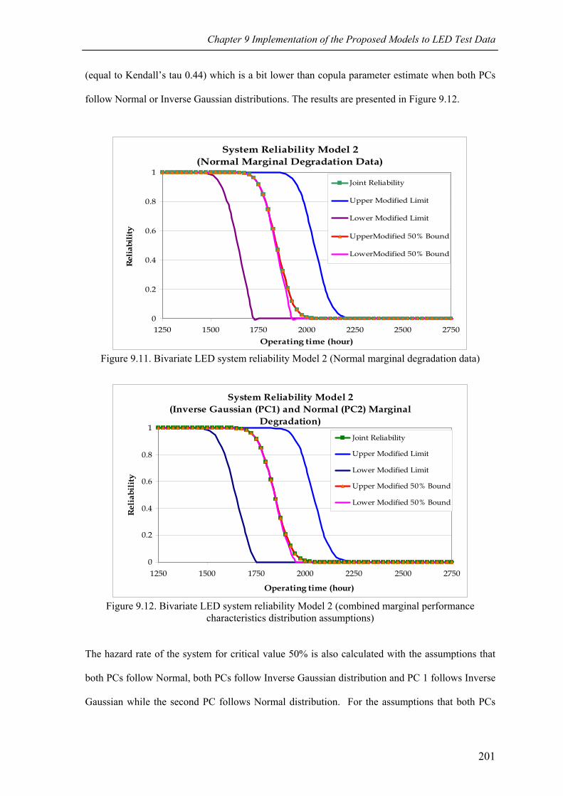
Chapter 9 Implementation of the Proposed Models to LED Test Data
(equal to Kendall’s tau 0.44) which is a bit lower than copula parameter estimate when both PCs
follow Normal or Inverse Gaussian distributions. The results are presented in Figure 9.12.
System Reliability Model 2(Normal Marginal Degradation Data)
0
0.2
0.4
0.6
0.8
1
1250 1500 1750 2000 2250 2500 2750Operating time (hour)
Rel
iabi
lity
Joint Reliability
Upper Modified Limit
Lower Modified Limit
UpperModified 50% Bound
LowerModified 50% Bound
Figure 9.11. Bivariate LED system reliability Model 2 (Normal marginal degradation data)
System Reliability Model 2(Inverse Gaussian (PC1) and Normal (PC2) Marginal
Degradation)
0
0.2
0.4
0.6
0.8
1
1250 1500 1750 2000 2250 2500 2750
Operating time (hour)
Rel
iabi
lity
Joint Reliability
Upper Modified Limit
Lower Modified Limit
Upper Modified 50% Bound
Lower Modified 50% Bound
Figure 9.12. Bivariate LED system reliability Model 2 (combined marginal performance
characteristics distribution assumptions)
The hazard rate of the system for critical value 50% is also calculated with the assumptions that
both PCs follow Normal, both PCs follow Inverse Gaussian distribution and PC 1 follows Inverse
Gaussian while the second PC follows Normal distribution. For the assumptions that both PCs
201

Chapter 9 Implementation of the Proposed Models to LED Test Data
are Normal and different marginal distributions, the hazard rates have very similar shapes with the
increase of the rate starts around 2000-hour. On the other hand, for both PCs follow Inverse
Gaussian distribution, the increase of the hazard rate starts just after 1600-hour with a hump and
increase again from 2000-hour. The results are presented in Figure 9.13-9.15.
Hazard Rate (Critical value 50% - Model 2)Normal Marginal Degradation Data
0
5
10
15
20
1500 2000 2500
Operating time (hour)
Haz
ard
rate
Figure 9.13. Hazard rate bivariate CSDT Model 2 (Normal marginal degradation data)
Hazard Rate (Critical value 50% - Model 2)Inverse Gaussian Marginal Degradation Data
0
0.005
0.01
0.015
0.02
0.025
0.03
1250 1500 1750 2000 2250
Operating time (hours)
Haz
ard
rate
Figure 9.14. Hazard rate bivariate CSDT Model 2 (Inverse Gaussian marginal degradation data)
Hazard Rate (Critical value 50% - Model 2)Inverse Gaussian (PC1) and Normal (PC2)
Marginal Degradation Data
0
2
4
6
8
10
12
1500 1750 2000 2250 2500
Operating time (hour)
Haz
ard
rate
Figure 9.15. Hazard rate bivariate CSDT Model 2 (combined marginal degradation distribution
assumptions)
202

Chapter 9 Implementation of the Proposed Models to LED Test Data
9.3.1.3. LED case study: Bivariate CSDT Model 3
In this analysis, random-effects are not included. Normal and Inverse Gaussian marginal
degradation data assumptions are used. The marginal degradation data of both PCs are also
modelled using simple linear functions. In general, the model can be written as,
Y = X.β + e
E(Y) = X.β
Var(Y) = V = T.Γ.T (9.8)
Just as Model 1, the correlation matrix has sub-matrices of the first and second PC with one-
dependent structure and sub-matrix of between PCs correlation with diagonal structure. However,
the standard deviation matrix T for Normal and Inverse Gaussian marginal degradation
distribution assumptions has different forms. Matrix T for Normal marginal distribution
assumption is a diagonal matrix with diagonal elements σk, which is not a function of time. On
the other hand, the diagonal elements of matrix T for Inverse Gaussian marginal distribution
assumption can be written as,
Tij(k) = σk . f(xij
(k).β(k)) = ( ) ( )
ijk
kkij
kkij
ta
xx
.
.. 23)()(2
3)()( β
λ
β= ; with i = j, and k = 1,2 (9.9)
Based on these assumptions and definitions, the unknown parameters of the degradation data
regression model can be estimated by performing the procedure of the stage-1 of bivariate CSDT
Model 3. The results are presented in Table 9.5.
These are used in stage-2 to estimate the copula parameter of the degradation data joint
distribution with assumption that the joint distribution can be modelled using Frank copula and
the copula parameter is not a function of time. Three critical value definitions (i.e. 30%, 40%,
and 50%) are analyzed. However, only the analysis for critical value 50% will be presented.
After performing stage-2 of bivariate CSDT Model 3, it is concluded that the copula parameter
203

Chapter 9 Implementation of the Proposed Models to LED Test Data
estimate for marginal data with Normal distribution assumption is 7.77 (= Kendall's tau 0.59)
while for Inverse Gaussian marginal degradation data assumption is 8.05 (= Kendall's tau 0.60).
Table 9.5. The results of stage-1 bivariate CSDT Model 3 Marginal Distribution Assumption
PC Component of the Model
Regression Function/Estimation
E(Y(1)) E(Y(1)) = 1.256 + 0.024. tij 1 Tij
(1) Tij(1) = σ1 = 2.377
E(Y(2)) E(Y(2)) = 3.051 + 0.025.tij
Normal Distribution
2 Tij
(2) Tij(2) = σ2 = 1.906
E(Y(1)) E(Y(1)) = 0.537 + 0.025.tij 1 σ1 σ1 = ijt0434.01
E(Y(2)) E(Y(2)) = 2.881 + 0.026.tij
Inverse Gaussian Distribution
2 σ2 σ2 = ijt0506.01
TTF - PDF (Critical value: 50% - Normal Marginal Degradation Data)
0
0.002
0.004
0.006
0.008
1500 1750 2000 2250 2500Operating time (hour)
PC 1PC 2Joint PDF
Figure 9.16.a. PDF of the TTF for Normal marginal degradation data (bivariate CSDT Model 3)
TTF - PDF (Critical value: 50% - Inverse Gaussian Marginal Degradation Data)
0
0.001
0.002
0.003
1250 1500 1750 2000 2250 2500Operating time (hour)
PC 1PC 2Joint PDF
Figure 9.16.b. PDF of the TTF for Inverse Gaussian marginal degradation data (bivariate CSDT
Model 3)
204

Chapter 9 Implementation of the Proposed Models to LED Test Data
The parameters of the model estimated at stage-1 and 2 are used to estimate the adjusted joint
PDF of the system's TTF, the reliability of the system (for critical value 50%) and system
reliability bounds and limits. The adjusted marginal PDFs show similar pattern to the results of
previous models that is the adjusted PDF of the second PC shows relatively shorter lifetime
compared to the marginal lifetime of the first PC. The adjusted joint PDF of the system also has
heavier right tail. However, the existence of the second peak (or hump) is more obvious in the
joint PDFs which are the results of Model 3 but all have similar operating time "location". These
marginal and joint PDF curves are shown in Figure 9.16 (a & b).
Interestingly, the reliability analysis (with critical value 50%) based on Model 3 yields relatively
similar reliability conclusion. Modified reliability bounds (based on the Kendall's tau
information) for critical value 50% and limits (for critical values 45% and 55%) are also
estimated. Figures 9.17 (a & b) present the results. The system reliability functions based on
both marginal distribution assumptions are almost overlap with the upper modified 50% bound
because the Kendall's tau is around 0.5 or more. Compared to the results of Model 1, the system
reliability with Normal marginal degradation assumption is a bit steeper than the one with Inverse
Gaussian assumption.
The hazard rate curves of the system for critical value 50% for both marginal degradation
distribution assumptions also have similar conclusion with the hazard rate curves calculated using
the other models. It increases around 2000-hour operating time. However, the hazard rate curves
calculated from the model with Normal marginal degradation data and Inverse Gaussian
assumptions have different peak times.
205
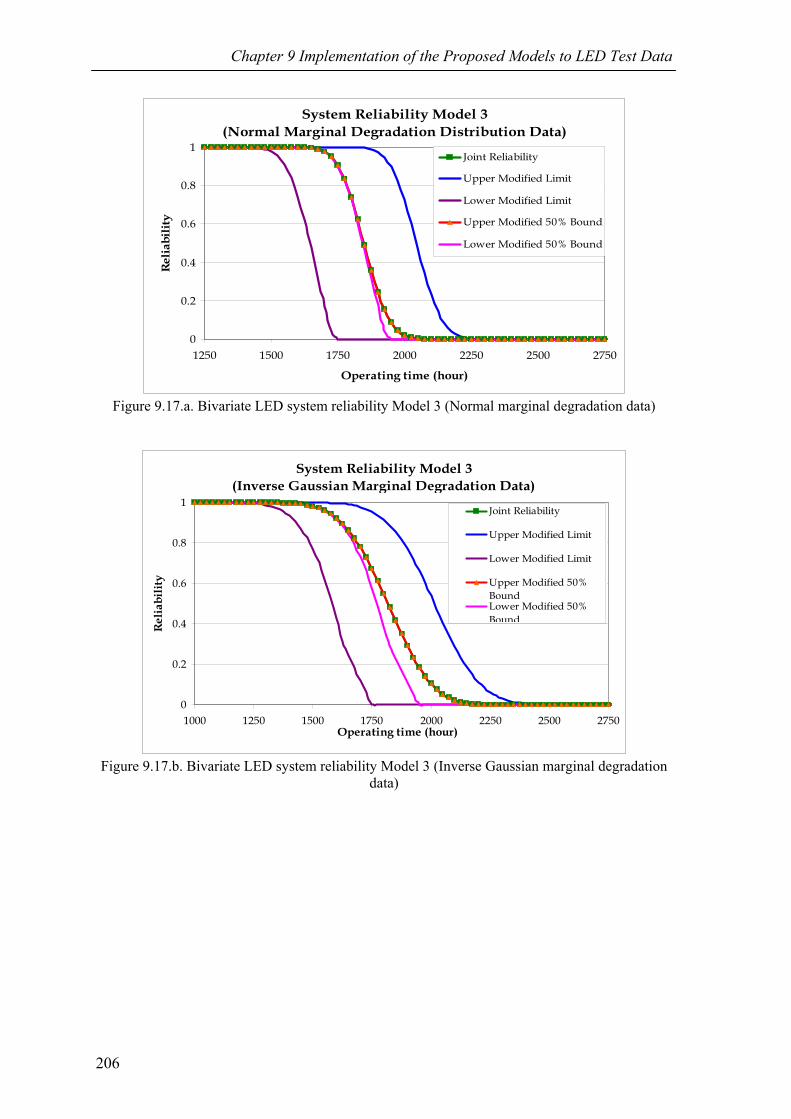
Chapter 9 Implementation of the Proposed Models to LED Test Data
System Reliability Model 3(Normal Marginal Degradation Distribution Data)
0
0.2
0.4
0.6
0.8
1
1250 1500 1750 2000 2250 2500 2750
Operating time (hour)
Rel
iabi
lity
Joint Reliability
Upper Modified Limit
Lower Modified Limit
Upper Modified 50% Bound
Lower Modified 50% Bound
Figure 9.17.a. Bivariate LED system reliability Model 3 (Normal marginal degradation data)
System Reliability Model 3(Inverse Gaussian Marginal Degradation Data)
0
0.2
0.4
0.6
0.8
1
1000 1250 1500 1750 2000 2250 2500 2750Operating time (hour)
Rel
iabi
lity
Joint Reliability
Upper Modified Limit
Lower Modified Limit
Upper Modified 50%BoundLower Modified 50%Bound
Figure 9.17.b. Bivariate LED system reliability Model 3 (Inverse Gaussian marginal degradation
data)
206

Chapter 9 Implementation of the Proposed Models to LED Test Data
Hazard Rate (Critical value 50% - Model 3)Normal Marginal Degradation Data
05
101520253035
1000 1500 2000 2500
Operating time (hours)
Haz
ard
rate
Figure 9.18.a. Hazard rate bivariate CSDT Model 3 (Normal marginal degradation data)
Hazard rate (Critical value 50% - Model 3)Inverse Gaussian Marginal Degradation Data
0
0.4
0.8
1.2
1.6
2
1000 1500 2000 2500 3000
Operating time (hour)
Haz
ard
rate
Figure 9.18.b. Hazard rate bivariate CSDT Model 3 (Inverse Gaussian marginal degradation data)
9.3.1.4. Bivariate CSDT Discussion
The comparisons between the proposed bivariate CSDT models have been presented in chapter
five. Therefore, in this sub-chapter, the discussion is focused on the implementation of these
models to the actual experimental data. From this implementation, it can be concluded that the
data may not comply nicely with the available theory. For example, it may be difficult to find a
parametric distribution function that best fit degradation data at all measurement times.
Therefore, trade-off should be considered when deciding the most suitable models and fitting the
experiment data. The consequences of this trade-off should be studied further to understand the
advantages and disadvantages of the decisions taken when modelling and analysing the
experiment data.
207

Chapter 9 Implementation of the Proposed Models to LED Test Data
An interesting thing that can be concluded from the bivariate CSDT example is that even though
the three proposed models result in different magnitude of conclusions, the results suggest similar
patterns and conclusions. These can be seen from the similar shape of the joint PDFs, similar
positive Kendall’s tau values, and similar system reliability and reliability bounds and limits.
However, different details of the conclusions may be found from the results of the three models.
Therefore, further study to explore the models in more detail analysis may be needed to obtain
better reliability profile analysis.
When a proposed model is applied to the data using different marginal distribution functions,
slightly different conclusions are obtained. However, the results of the use of different marginal
distribution functions with a bivariate CSDT model still in general demonstrate similar behaviour.
This is quite interesting to be studied further. This means that even though in details different
marginal distribution assumptions will result in different detail conclusions, they might still result
in similar general conclusions.
Besides what have been discussed, another interesting point is the hazard rate. It shows the
indication of the third and fourth phases of the roller-coaster curve. This means that the
experimental data demonstrates the aging of the system. This gives conformation the notion that
LED lamp has degradation failure mechanism. Although it gives this confirmation, further study
should be done to obtain more understanding of the failure behaviour of the LED lamps since
influx of technology in this area is quite high.
9.3.2. Multivariate CSDT Modelling and Analysis
The second case study is multivariate CSDT modelling and analysis. In order to illustrate this,
more than two failure mechanisms (or PCs) are needed. The data of the low power LED tube
lights used in the bivariate CSDT case study will be used as the first and second PCs. In addition,
the degradation data from the high power LED light bulb test will be assumed as the third and
208
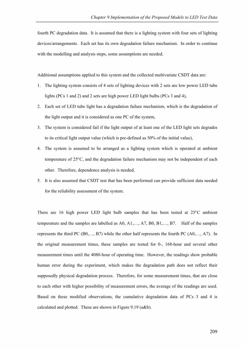
Chapter 9 Implementation of the Proposed Models to LED Test Data
fourth PC degradation data. It is assumed that there is a lighting system with four sets of lighting
devices/arrangements. Each set has its own degradation failure mechanism. In order to continue
with the modelling and analysis steps, some assumptions are needed.
Additional assumptions applied to this system and the collected multivariate CSDT data are:
1. The lighting system consists of 4 sets of lighting devices with 2 sets are low power LED tube
lights (PCs 1 and 2) and 2 sets are high power LED light bulbs (PCs 3 and 4),
2. Each set of LED tube light has a degradation failure mechanism, which is the degradation of
the light output and it is considered as one PC of the system,
3. The system is considered fail if the light output of at least one of the LED light sets degrades
to its critical light output value (which is pre-defined as 50% of the initial value),
4. The system is assumed to be arranged as a lighting system which is operated at ambient
temperature of 25°C, and the degradation failure mechanism may not be independent of each
other. Therefore, dependence analysis is needed,
5. It is also assumed that CSDT test that has been performed can provide sufficient data needed
for the reliability assessment of the system.
There are 16 high power LED light bulb samples that has been tested at 25°C ambient
temperature and the samples are labelled as A0, A1,…, A7, B0, B1,…, B7. Half of the samples
represents the third PC (B0,…, B7) while the other half represents the fourth PC (A0,…, A7). In
the original measurement times, these samples are tested for 0-, 168-hour and several other
measurement times until the 4080-hour of operating time. However, the readings show probable
human error during the experiment, which makes the degradation path does not reflect their
supposedly physical degradation process. Therefore, for some measurement times, that are close
to each other with higher possibility of measurement errors, the average of the readings are used.
Based on these modified observations, the cumulative degradation data of PCs 3 and 4 is
calculated and plotted. These are shown in Figure 9.19 (a&b).
209

Chapter 9 Implementation of the Proposed Models to LED Test Data
Cumulative Degradation at 25C - PC 3
0
10
20
30
40
50
60
70
0 1000 2000 3000 4000
Operating time (hour)
Cum
ulat
ive
Deg
rada
tion
(%)
B0B1B2B3B4B5B6B7Avg
Figure 9.19.a. Performance characteristic 3 cumulative degradation curve at 25°C
Cumulative Degradation at 25C - PC 4
-10
0
10
20
30
40
50
60
0 1000 2000 3000 4000
Operating time (hour)
Cum
ulat
ive
Deg
rada
tion
(%)
A0A1A2A3A4A5A6A7Avg
Figure 9.19.b. Performance characteristic 4 cumulative degradation curve at 25°C
Since the data points that can be used to model the third and fourth PCs are now lesser,
consequently lesser unknown variables can be estimated if the efficiency of the estimation wants
to be maintained. Therefore, Normal distribution with two parameters (μ and σ) will be used to
model the marginal degradation data distribution of these two PCs. It is also assumed that the
standard deviation (σ) of the marginal degradation data of PCs 3 and 4 is not a function of time.
210
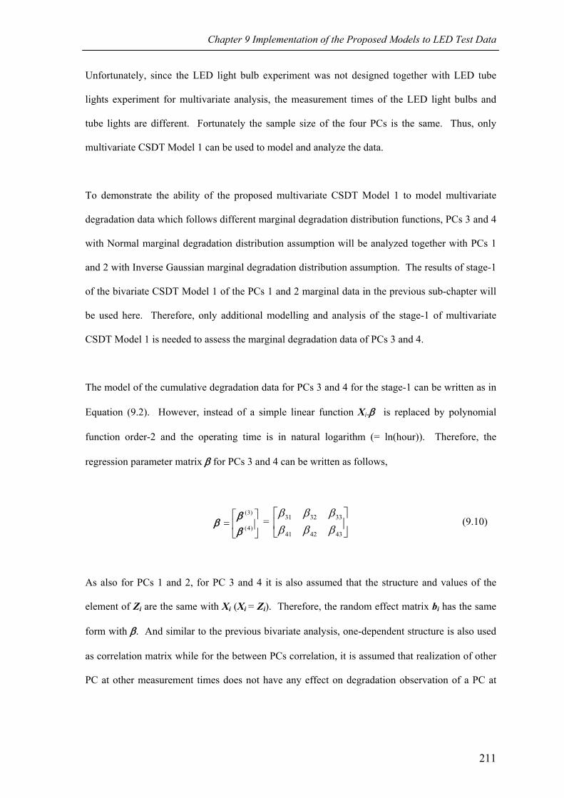
Chapter 9 Implementation of the Proposed Models to LED Test Data
Unfortunately, since the LED light bulb experiment was not designed together with LED tube
lights experiment for multivariate analysis, the measurement times of the LED light bulbs and
tube lights are different. Fortunately the sample size of the four PCs is the same. Thus, only
multivariate CSDT Model 1 can be used to model and analyze the data.
To demonstrate the ability of the proposed multivariate CSDT Model 1 to model multivariate
degradation data which follows different marginal degradation distribution functions, PCs 3 and 4
with Normal marginal degradation distribution assumption will be analyzed together with PCs 1
and 2 with Inverse Gaussian marginal degradation distribution assumption. The results of stage-1
of the bivariate CSDT Model 1 of the PCs 1 and 2 marginal data in the previous sub-chapter will
be used here. Therefore, only additional modelling and analysis of the stage-1 of multivariate
CSDT Model 1 is needed to assess the marginal degradation data of PCs 3 and 4.
The model of the cumulative degradation data for PCs 3 and 4 for the stage-1 can be written as in
Equation (9.2). However, instead of a simple linear function Xi.β is replaced by polynomial
function order-2 and the operating time is in natural logarithm (= ln(hour)). Therefore, the
regression parameter matrix β for PCs 3 and 4 can be written as follows,
(3)
(4)
⎡ ⎤= ⎢ ⎥⎣ ⎦
ββ
β = (9.10) ⎥
⎦
⎤⎢⎣
⎡
434241
333231
ββββββ
As also for PCs 1 and 2, for PC 3 and 4 it is also assumed that the structure and values of the
element of Zi are the same with Xi (Xi = Zi). Therefore, the random effect matrix bi has the same
form with β. And similar to the previous bivariate analysis, one-dependent structure is also used
as correlation matrix while for the between PCs correlation, it is assumed that realization of other
PC at other measurement times does not have any effect on degradation observation of a PC at
211

Chapter 9 Implementation of the Proposed Models to LED Test Data
certain measurement time. The results of the stage-1 of multivariate CSDT Model 1 for the fixed-
effect of the PCs 3 and 4 are presented in Table 9.6.
Table 9.6. The results of stage-1 multivariate CSDT Model 1 for PC 3 and 4
Performance Characteristic
Distribution Parameter
Regression Function/Estimation
μ3 μ3 = 0.048 - 2.7842737.ln(t) + 0.904.(ln(t))2 3 σ3 9.997679 μ4 μ3 = 0.903 - 4.41.ln(t) + 1.06.(ln(t))2 4 σ4 9.900535
As in the previous sub-chapter, the random-effects bi can then be calculated using (5.14). These
are used to predict the TTFs of PCs 3 and 4 which are listed in Table 9.7.
Table 9.7. Predicted TTF data (hours) of PCs 3 and 4 with critical value 50% PC 3 PC 4 Sample
μ = 9226.15; σ = 391.478 μ = 9683.83; σ = 237.135 1 8859 9461 2 9023 9562 3 8811 9431 4 9379 9778 5 9725 9984 6 9685 9962 7 8822 9438 8 9506 9853
Recall from the previous sub-chapter, that for the predicted TTF data of PCs 1 and 2, Birnbaum-
Saunders distribution is used to represents the distribution of predicted marginal TTF data. For
PCs 3 and 4, Normal distribution will be used to represent the distribution of their predicted
marginal TTF data. The estimated distribution parameters are also listed in Table 9.7. Normal
distribution assumption is chosen to demonstrate that the analysis can be done with the model
when the data has different marginal distribution functions.
To continue with the analysis of stage-2, multivariate copula function is needed. Assume that
exchangeable multivariate Frank copula (refer to Equation 6.9) is suitable to model the
multivariate predicted TTF data. Based on this assumption, stage-2 of the multivariate CSDT
Model 1 is performed and the copula parameter is predicted. It results in Frank copula parameter,
212

Chapter 9 Implementation of the Proposed Models to LED Test Data
θ = 3.65 which is approximately equal to Kendall's tau 0.36. This corresponds to the general
dependence effect of the 4-variate degradation failure.
The result that has been gathered is used to estimate the marginal and system reliability functions
using Equation (6.18) or (6.20) will be used. The result is shown in Figure 9.20. This figure
shows that the independent and dependent system reliability estimates are quite close to the
marginal reliability of PC 2, which has the lowest reliability compared to the other three marginal
PCs. The system reliability which uses Frank copula to model the joint distribution has generally
higher reliability value than independent system reliability. This is because the copula parameter
is found to be positive. This shows that using independent assumption may give different system
reliability conclusion when there is actually dependency between PCs in the system.
The marginal PDFs of PCs 3 and 4 are plotted in Figure 9.21. This figure shows that the marginal
PDF of PCs 3 and 4 are far at the right side of PCs 1 and 2. This supports the conclusion of
Figure 9.20 that the marginal reliability estimates of PCs 3 and 4 are significantly higher than PCs
1 and 2. Therefore, the first and second failure mechanisms may have stronger influence on the
system reliability. The adjusted system PDF is also presented in Figure 9.22. It shows that the
peak of the failure probability is much closer to the first and second PCs than to the third and
fourth PCs.
Meanwhile, the hazard rate of the multivariate degradation data also shows similar conclusion to
the previous sub-chapter. The degradation data of the LED lamps system reflects part of the third
and fourth phases of the roller-coaster curve. This shows that the main failure mechanism in the
system is aging. This information can be used to plan and analyze the policy of the company
related to the particular system.
213

Chapter 9 Implementation of the Proposed Models to LED Test Data
System Reliability (Critical value 50%)Inverse Gaussian and Normal Marginal Degradation Data
0
0.2
0.4
0.6
0.8
1
1000 2000 3000 4000 5000 6000 7000 8000 9000 10000 11000
Operating time (hours)
Rel
iabi
lity
R1
R2
R3
R4
DependentSystemReliabilityIndependentSystemReliability
Figure 9.20. System reliability of multivariate degraded system
Marginal PDF - PC 3 & 4 (Critical value 50%)Normal Marginal Degradation Data
0
0.0005
0.001
0.0015
0.002
7000 8000 9000 10000 11000
Operating time (hours)
PC 3
PC 4
Figure 9.21. Marginal PDF of the TTF for performance characteristics 3 and 4
Joint PDF (Crirical value 50%)
Inverse Gaussian (PC 1 and 2) and Normal (PC 3 and 4) Marginal Degradation Data
0
0.002
0.004
0.006
0.008
2000 2500 3000 3500Operating time (hours)
Figure 9.22. Joint PDF of the multivariate degraded system
214

Chapter 9 Implementation of the Proposed Models to LED Test Data
Multivariate LED System Hazard rate (critical value 50%)
0.E+00
1.E+10
2.E+10
3.E+10
4.E+10
1500 2000 2500Operating time (hour)
Haz
ard
rate
Figure 9.23. Hazard rate of the multivariate degraded system
9.3.3. Bivariate CSADT Modelling and Analysis
Consider the same lighting system (low power LED tube lights) as the first case study in sub-
chapter 9.3.1. However, this case study, the degradation data is originated from a bivariate
CSADT. Because of the constraints discussed in the beginning of this chapter, there are only 2
stress levels at which the samples are tested. In addition, as presented in sub-chapter 9.2.3,
because of some unexpected catastrophic failures which are occurred during the test at high level
stress, for each PC at each stress level only 7 samples that will be included as the degradation
data. The general assumptions of the bivariate system (1-4) in sub-chapter 9.3.1 are also valid
here except assumption no. 5. In addition, it will be assumed that reliability evaluation of the
system at environment temperature of 40°C is needed.
The cumulative degradation data of the first and second PCs at 25°C and 55°C is presented at
Figures 9.24 and 9.25. These curves show relatively linear degradation paths. Therefore, for both
PCs and both stress levels, the degradation paths may be modelled using simple linear functions.
215

Chapter 9 Implementation of the Proposed Models to LED Test Data
Cumulative Degradation at 25C - PC 1
-5%
0%
5%
10%
15%
20%
25%
30%
0:00 240:00 480:00 720:00 960:00
Operating time (Hour)
Cum
ulat
ive
Deg
rada
tion
1
2
3
4
5
6
7
Avg
Figure 9.24.a. Performance characteristic 1 cumulative degradation curve at 25°C (low stress
level)
Cumulative Degradation at 25C - PC 2
0%
5%
10%
15%
20%
25%
30%
0:00 240:00 480:00 720:00 960:00Operating time (Hour)
Cum
ulat
ive
Deg
rada
tion
1
2
3
4
5
6
7
Avg
Figure 9.24.b. Performance characteristic 2 cumulative degradation curve at 25°C (low stress
level)
Cumulative Degradation at 55C - PC 1
0%
5%
10%
15%
20%
25%
30%
35%
40%
0:00 240:00 480:00 720:00 960:00
Operating time (Hour)
Cum
ulat
ive
Deg
rada
tion
1
2
3
4
5
6
7
Avg
Figure 9.25.a. Performance characteristic 1 cumulative degradation curve at 55°C (high stress
level)
216

Chapter 9 Implementation of the Proposed Models to LED Test Data
Cumulative Degradation at 55C - PC 2
-5%
0%
5%
10%
15%
20%
25%
30%
35%
40%
0:00 240:00 480:00 720:00 960:00
Operating time (Hour)
Cum
ulat
ive
Deg
rada
tion
1
2
3
4
5
6
7
Avg
Figure 9.25.b. Performance characteristic 2 cumulative degradation curve at 55°C (high stress
level)
Analysis of the possible marginal degradation distribution functions is performed to this bivariate
CSADT data. Based on the AIC values, Inverse Gaussian distribution fits best to both PCs 1 and
2 at most measurement times at both stress levels. However, considering that the relationships
between the stress levels and certain parameters of the degradation models have not been well
developed and the results of the three proposed bivariate CSADT models will be compared,
Normal distribution is chosen to represent the marginal degradation distribution of both PCs at all
stress levels. The analysis of the data is represented in the following sub-chapters.
9.3.3.1. LED case study: Bivariate CSADT Model 1
Simple linear function will be used to model the two PCs at both stress levels. The model for the
cumulative degradation data of this system that will be used in the first stage of bivariate CSADT
Model 1 can be written as Equation (9.2). In the stage 1 of the bivariate CSADT Model 1,
cumulative degradation data of each PC at each stress level is analyzed. The unknown parameters
of the fixed-effects components of the marginal degradation model are estimated and tabulated in
Table 9.8. The estimated random-effects components of the models are not shown.
217

Chapter 9 Implementation of the Proposed Models to LED Test Data
Table 9.8. The results of stage 1 bivariate CSADT Model 1 Stress Level PC Component of
the Model Regression Function/Estimation
E(Y(1)) E(Y(1)) = 1.92 + 0.024. tij 1 Tij
(1) Tij(1) = σ1 = 0.937
E(Y(2)) E(Y(2)) = 3.189 + 0.026.tij
25°C
2 Tij
(2) Tij(2) = σ2 = 1.078
E(Y(1)) E(Y(1)) = 5.03 + 0.031.tij 1 Tij
(1) Tij
(1) = σ1 = 2.5 E(Y(2)) E(Y(2)) = 5.62 + 0.03.tij
55°C
2 Tij
(2) Tij
(2) = σ2 = 4.37
The estimated parameters shown in Table 9.8 are used together with the estimated random-effects
parameters to predict the TTFs of each sample of each PC at each stress level. This is done for
the assumed critical value of 30%, 40% and 50% for both PCs. However, only the analysis with
the critical value of 50% is presented in details. The predicted TTF data is shown at Table 9.9.
Stage 2 of the bivariate CSADT Model 1 can be performed after obtaining this predicted TTFs
data. The second stage is started by analyzing the predicted TTFs data and possible distribution
function to model the data. The important assumption to remember is that each PC follows the
same marginal TTF distribution function at all stress levels. Based on this assumption and
considering the distribution that is widely-used to model TTF data, Weibull distribution is chosen
to model TTFs of both PCs.
Table. 9.9. Predicted TTFs data (hours): critical value 50%, CSADT Model 1
Stress level 25°C Stress level 55°C Sample PC 1 PC 2 PC 1 PC 2
1 1879 1798 1480 1482 2 2727 1788 1425 1417 3 2062 1973 1471 1388 4 1875 1650 1321 1550 5 1969 1822 1517 1555 6 2070 1858 1502 1479 7 1947 1728 1484 1350
By doing separate MLE analysis with assumption that the TTF follow Weibull distribution, the
estimation of the Weibull distribution parameters for each PC at each stress level can be obtained.
The estimation of the parameter α (scale parameter) is 2205.47 and 1847.73 for PC 1 and 2
respectively and the estimation of parameter β (shape parameter) is 6.66 and 19.78 for PC 1 and 2
218

Chapter 9 Implementation of the Proposed Models to LED Test Data
respectively at 25°C. The estimation of the parameter α (scale parameter) is 1482.39 and 1494.59
for PC 1 and 2 respectively and the estimation of parameter β (shape parameter) is 37.37 and
23.15 for PC 1 and 2 respectively at 55°C.
In the stage 2 of the bivariate CSADT Model 1, relationship models between the stress level and
TTF distribution parameters are needed. The following relationships are used with consideration
to Arrhenius model because temperature (T) is used to accelerate the test and also to avoid getting
non-positive parameters value,
( )T16.273
1000.ln 11 ++= baα
( ) T.ln 22 ba +=β (9.11)
Performing estimation method using MLE, similar to the commonly-used estimation of the
unknown parameters in the TTF distribution parameters-stress in ALT, the unknown parameters
at Equation (9.11) can be obtained. The estimated parameters for PC 1 are: a1 = 3.35, b1 = 1.3, a2
= 0.46, b2 = 0.057. Meanwhile, the estimated parameters for PC 2 are: a1 = 5.2, b1 = 0.69, a2 =
2.85, b2 = 0.005. These estimated parameters are used to find the estimated TTF distribution
parameters at 40°C. The estimated TTF distribution parameters at 40°C will then be used to
predict the reliability of the system when the system is operated at 40°C.
Before reliability of the system at 40°C is predicted, the first thing that should be done in the stage
3 of the bivariate CSADT Model 1 is to find the copula parameter which is valid at the
operational condition. As the previous case studies, it is assumed that Frank copula is appropriate
to couple the marginal and bivariate distribution functions. It is also assumed that the copula
parameter (θ) is a function of the temperature and can be model as follows,
θ = a3 + b3.T (9.12)
219

Chapter 9 Implementation of the Proposed Models to LED Test Data
Using IFM method and predicted TTFs data, parameter a3 and b3 are estimated to be 2.207 and -
0.038 respectively. Based on these, the copula parameter at 40°C is estimated to be 0.67 or equal
to Kendall’s tau 0.07.
This information is used to perform stage 3 of the bivariate CSADT Model 1. First, estimate the
TTF distribution parameters of PCs 1 and 2 at 40°C. The estimated distribution parameters α and
β for PC 1 are 1070.99 and 15.78 respectively and for PC 2 are 1653.4 and 21.4 respectively.
Based on this, the marginal reliability, system reliability, system PDF and reliability bounds at
40°C can be estimated. The results are presented in Figures 9.26 – 9.28.
PDF - Critical value 50%, Temp. 40C
0
0.001
0.002
0.003
0.004
0.005
0.006
750 1000 1250 1500 1750 2000 2250
Operating time (Hours)
PC 1
PC 2Joint PDF
Figure 9.26. Bivariate CSADT PDF with critical value 50% at 40°C Model 1
The marginal PDF curves show that the second PC is relatively more severe than the first PC.
Both PCs have left tail. This tail is also reflected at the adjusted system PDF. While in Figure
9.27, it can be seen that since the copula parameter ≈ 0, the difference between independent and
dependent system reliability is not very obvious. However, the dependent system reliability is
relatively higher than the independent system reliability because the copula parameter is positive.
Upper and lower reliability limits are calculated with assumption that the critical values range
between 45% - 55%. These limits cover wider area than the system reliability bounds calculated
220

Chapter 9 Implementation of the Proposed Models to LED Test Data
based on the assumptions that the critical value is 50% and using Kendall’s tau bounds
improvement formula. Both reliability limits and reliability bounds provide illustration of the
possible uncertainty of the assumptions and model.
System Reliability - Critical value 50%, Temp. 40C
0
0.2
0.4
0.6
0.8
1
1000 1250 1500 1750 2000 2250Operating time (Hours)
Rel
iabi
lity
PC 1
PC 2
Independent SystemReliabilityDependent SystemReliability
Figure 9.27. Marginal and system reliability with critical value 50% at 40°C Model 1
System Reliability - Critical value 50%, Temp. 40C
0
0.2
0.4
0.6
0.8
1
1000 1250 1500 1750 2000 2250 2500
Operating time (Hours)
Rel
iabi
lity
Independent SystemReliabilityDependent SystemReliabilityModified UpperReliability LimitModified LowerReliability LimitUpper ReliabilityKendall's 50% BoundLower ReliabilityKendall's 50% Bound
Figure 9.28. System reliability and reliability bounds and limits at 40°C Model 1
221

Chapter 9 Implementation of the Proposed Models to LED Test Data
Hazard Function - Critical value 50%Temp. 40C
0
1
2
3
4
5
1000 1250 1500 1750 2000
Operating time (Hours)
Haz
ard
rate
Figure 9.29. Hazard rate for critical value 50% and temperature 40°C Model 1
The hazard rate of the system at operational temperature 40°C is also obtained. Similar to the
previous case studies, it also shows the third and fourth phases of the roller-coaster curve. This is
in line with the theory of aging/degraded system.
9.3.3.2. LED case study: Bivariate CSADT Model 2
As the previous sub-chapter, assume that both marginal degradation data follow Normal
distribution function. In Mode 2, the marginal distribution parameters at each measurement times
and each stress level are estimated first using MLE procedure. Then, GLM is applied to these
estimated parameters. On the contrary to Mode 1, the relationships between the data at different
stress levels and the stress levels should be defined in the first stage. These relationships are
substituted to the marginal distribution parameters regression functions. It is assumed that the
mean (μ) of the marginal distribution is a function of time. The slope of this function is assumed
to be a function of the stress level. It means that the degradation rate depends on the stress level.
The standard deviation (σ) of the marginal distribution is assumed to be a function of the stress
level (s) but not a function of time. The GLM of the mean parameter (μ) can now be written as
follows,
U = X.β + e
E(U) = X.β = β1 + β2.tj
β2 = β2a + β2b.s
Var(U) = V = T.Γ.T (9.13)
222

Chapter 9 Implementation of the Proposed Models to LED Test Data
Where s is the stress level (= temperature). It is decided not to use the usual Arrhenius model in
order to have simpler model and also because the real model that suit the acceleration of the LED
lamp test is not known yet. Therefore, it is decided to use a simple model to simplify the
illustration and calculation. The correlation matrix of Equation (9.13) is assumed to be one-
dependent structure. Meanwhile, for the standard deviation (σ) of the marginal distribution is
modelled as follows,
σ = exp(a1 + a2.s) (9.14)
After performing the procedure of the stage 1 bivariate CSADT Model 2, the unknown parameters
of the model can be obtained. They are presented in Table 9.10. These are used in stage 2 to
estimate the copula parameter at each stress level and the at the stress level at which we would
like to assess the system reliability. As all models in this thesis, Frank copula is assumed suitable
to model the system.
Table 9.10. The results of stage 1 bivariate CSADT Model 2
PC Component of the Model Regression Function/Estimation μ(1) μ(1) = 2 + β12. tij β12 β12 = 0.01 + 0.00039.T
1
σ (1) σ (1) = exp(1.3 + -0.015.T) μ(2)
μ(2) = 3.5 + β22.tij
β22 β22 = 0.01 + 0.00061.T 2
σ (2) σ (2) = exp(-0.584 + 0.0212.T)
Using IFM and with assumption that the copula parameter is not a function of time but is a
function of the stress level (temperature) as Equation (9.12), the copula parameter at 25°C and
55°C and the unknown parameters of its relationship with temperature are estimated. The
relationship between the copula parameter and temperature can be written as follows,
θ = 7.17 – 0.2T (9.15)
In the stage 3, the marginal and system PDF and reliability at operational temperature 40°C can
be estimated with assumption that the critical value is 50% for both PCs. This is done with
223

Chapter 9 Implementation of the Proposed Models to LED Test Data
copula parameter (θ) = -0.8 which is approximately equal to Kendall’s tau -0.09. The adjusted
marginal and joint PDF curves are presented in Figure 9.30. As the conclusion of the previous
model, the second PC is relatively more severe than the first one. However, compared to the
result of Model 1, the PDFs obtained by this model have relatively narrower deviation and more
symmetric. This may be the result of using Normal distribution to model the marginal
degradation data. However, they still have similar general pattern to the result of Model 1.
As can be expected the marginal reliability of the first PC is relatively higher than the second PC.
The estimated system reliability, modified reliability limits based on the Kendall’s tau value and
the reliability bounds for critical value 50% and Kendall’s tau value at 40°C can be calculated.
They are presented in Figure 9.31. Since the Kendall’s tau is ≈ 0, the reliability bounds for
critical value 50% almost coincide with the system reliability. The modified upper and lower
reliability limits are calculated with assumption that the upper and lower critical value limits are
45% and 55% respectively.
PDF (Critical value 50%, Temp. 40C)ADT Model 2
0
0.004
0.008
0.012
750 1250 1750 2250Operating Time (Hours)
PC1PC2Joint PDF
Figure 9.30. Bivariate CSADT PDF with critical value 50% at 40°C Model 2
The hazard rate also shows aging sign of the system. However, it reaches the peak at earlier
operating time than when it is calculated using bivariate CSADT Model 1.
224
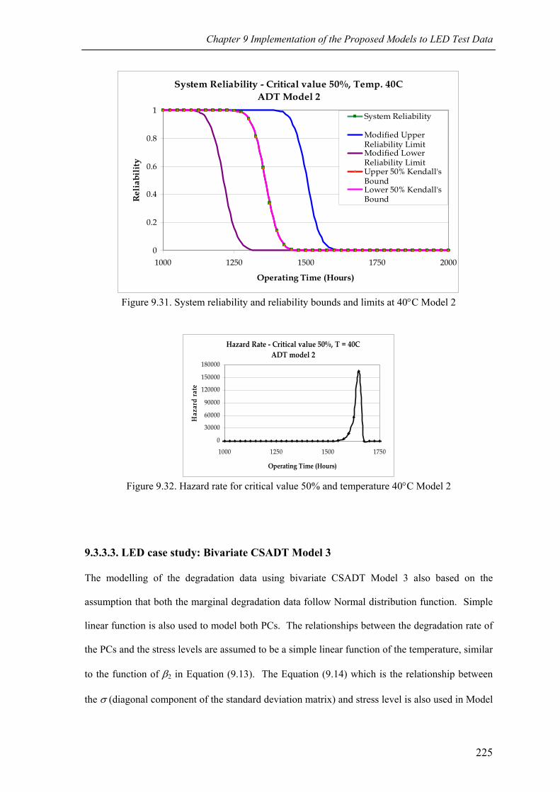
Chapter 9 Implementation of the Proposed Models to LED Test Data
System Reliability - Critical value 50%, Temp. 40CADT Model 2
0
0.2
0.4
0.6
0.8
1
1000 1250 1500 1750 2000
Operating Time (Hours)
Rel
iabi
lity
System Reliability
Modified UpperReliability LimitModified LowerReliability LimitUpper 50% Kendall'sBoundLower 50% Kendall'sBound
Figure 9.31. System reliability and reliability bounds and limits at 40°C Model 2
Hazard Rate - Critical value 50%, T = 40C ADT model 2
0
30000
60000
90000
120000
150000
180000
1000 1250 1500 1750
Operating Time (Hours)
Haz
ard
rate
Figure 9.32. Hazard rate for critical value 50% and temperature 40°C Model 2
9.3.3.3. LED case study: Bivariate CSADT Model 3
The modelling of the degradation data using bivariate CSADT Model 3 also based on the
assumption that both the marginal degradation data follow Normal distribution function. Simple
linear function is also used to model both PCs. The relationships between the degradation rate of
the PCs and the stress levels are assumed to be a simple linear function of the temperature, similar
to the function of β2 in Equation (9.13). The Equation (9.14) which is the relationship between
the σ (diagonal component of the standard deviation matrix) and stress level is also used in Model
225
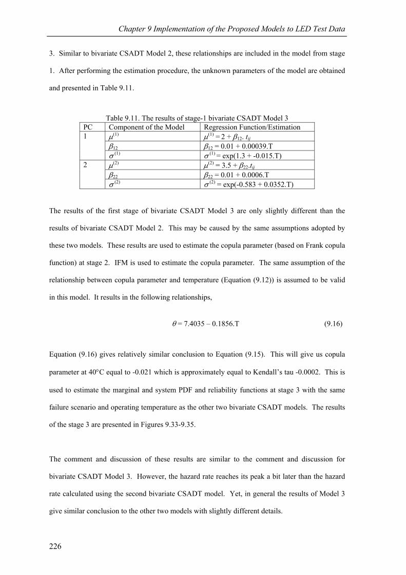
Chapter 9 Implementation of the Proposed Models to LED Test Data
3. Similar to bivariate CSADT Model 2, these relationships are included in the model from stage
1. After performing the estimation procedure, the unknown parameters of the model are obtained
and presented in Table 9.11.
Table 9.11. The results of stage-1 bivariate CSADT Model 3 PC Component of the Model Regression Function/Estimation
μ(1) μ(1) = 2 + β12. tij β12 β12 = 0.01 + 0.00039.T
1
σ (1) σ (1) = exp(1.3 + -0.015.T) μ(2)
μ(2) = 3.5 + β22.tij
β22 β22 = 0.01 + 0.0006.T 2
σ (2) σ (2) = exp(-0.583 + 0.0352.T)
The results of the first stage of bivariate CSADT Model 3 are only slightly different than the
results of bivariate CSADT Model 2. This may be caused by the same assumptions adopted by
these two models. These results are used to estimate the copula parameter (based on Frank copula
function) at stage 2. IFM is used to estimate the copula parameter. The same assumption of the
relationship between copula parameter and temperature (Equation (9.12)) is assumed to be valid
in this model. It results in the following relationships,
θ = 7.4035 – 0.1856.T (9.16)
Equation (9.16) gives relatively similar conclusion to Equation (9.15). This will give us copula
parameter at 40°C equal to -0.021 which is approximately equal to Kendall’s tau -0.0002. This is
used to estimate the marginal and system PDF and reliability functions at stage 3 with the same
failure scenario and operating temperature as the other two bivariate CSADT models. The results
of the stage 3 are presented in Figures 9.33-9.35.
The comment and discussion of these results are similar to the comment and discussion for
bivariate CSADT Model 3. However, the hazard rate reaches its peak a bit later than the hazard
rate calculated using the second bivariate CSADT model. Yet, in general the results of Model 3
give similar conclusion to the other two models with slightly different details.
226
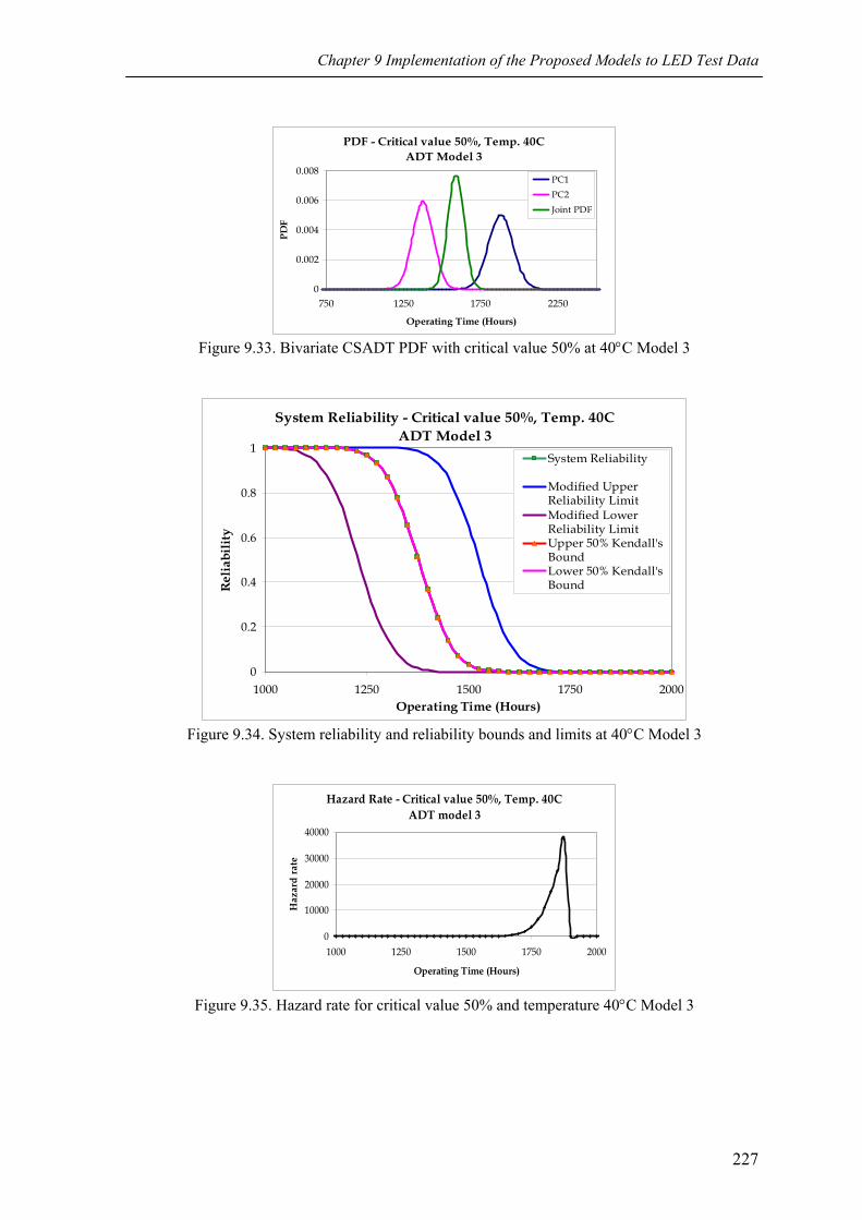
Chapter 9 Implementation of the Proposed Models to LED Test Data
PDF - Critical value 50%, Temp. 40CADT Model 3
0
0.002
0.004
0.006
0.008
750 1250 1750 2250
Operating Time (Hours)
PC1PC2Joint PDF
Figure 9.33. Bivariate CSADT PDF with critical value 50% at 40°C Model 3
System Reliability - Critical value 50%, Temp. 40CADT Model 3
0
0.2
0.4
0.6
0.8
1
1000 1250 1500 1750 2000Operating Time (Hours)
Rel
iabi
lity
System Reliability
Modified UpperReliability LimitModified LowerReliability LimitUpper 50% Kendall'sBoundLower 50% Kendall'sBound
Figure 9.34. System reliability and reliability bounds and limits at 40°C Model 3
Hazard Rate - Critical value 50%, Temp. 40C
ADT model 3
0
10000
20000
30000
40000
1000 1250 1500 1750 2000
Operating Time (Hours)
Haz
ard
rate
Figure 9.35. Hazard rate for critical value 50% and temperature 40°C Model 3
227
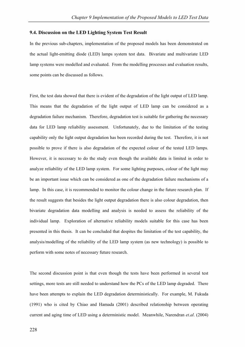
Chapter 9 Implementation of the Proposed Models to LED Test Data
9.4. Discussion on the LED Lighting System Test Result
In the previous sub-chapters, implementation of the proposed models has been demonstrated on
the actual light-emitting diode (LED) lamps system test data. Bivariate and multivariate LED
lamp systems were modelled and evaluated. From the modelling processes and evaluation results,
some points can be discussed as follows.
First, the test data showed that there is evident of the degradation of the light output of LED lamp.
This means that the degradation of the light output of LED lamp can be considered as a
degradation failure mechanism. Therefore, degradation test is suitable for gathering the necessary
data for LED lamp reliability assessment. Unfortunately, due to the limitation of the testing
capability only the light output degradation has been recorded during the test. Therefore, it is not
possible to prove if there is also degradation of the expected colour of the tested LED lamps.
However, it is necessary to do the study even though the available data is limited in order to
analyze reliability of the LED lamp system. For some lighting purposes, colour of the light may
be an important issue which can be considered as one of the degradation failure mechanisms of a
lamp. In this case, it is recommended to monitor the colour change in the future research plan. If
the result suggests that besides the light output degradation there is also colour degradation, then
bivariate degradation data modelling and analysis is needed to assess the reliability of the
individual lamp. Exploration of alternative reliability models suitable for this case has been
presented in this thesis. It can be concluded that despites the limitation of the test capability, the
analysis/modelling of the reliability of the LED lamp system (as new technology) is possible to
perform with some notes of necessary future research.
The second discussion point is that even though the tests have been performed in several test
settings, more tests are still needed to understand how the PCs of the LED lamp degraded. There
have been attempts to explain the LED degradation deterministically. For example, M. Fukuda
(1991) who is cited by Chiao and Hamada (2001) described relationship between operating
current and aging time of LED using a deterministic model. Meanwhile, Narendran et.al. (2004)
228
Chapter 9 Implementation of the Proposed Models to LED Test Data
use an exponential function to describe the LED’s light output degradation over time. In their
published paper, Parker et.al. (1999) show some degradation paths of polymer LED under
different operational temperatures. The light intensity of the polymer LEDs is first increasing and
after it reaches a peak, it starts to decrease. In the Handbook of Advanced Electronic and
Photonic Material and Devices (2001), it is suggested that the degradation behaviour of LED may
be influenced by several external factors for instance oxidation, photo-oxidation, diffusion of the
electrode and effect of heat, while Narendran et.al. (2001) list junction temperature as the most
important factor that influences LED degradation behaviour. This means that the degradation
behaviour of LED as a lighting source will depend on the LED technology used in the lamp and
design of the lamp. With the influx of new LED technology and new LED lamp designs, it means
that while an experiment is performed to understand failure behaviour of certain LED lamp
type/design, there are likely new LED lamp designs with different failure behaviour introduced
into the market. Therefore, more tests should be done and database of LED lamps degradation
behaviour should be build for research purposes.
The light output data monitored during the experiment, shows that for both type of LED lamp
tested, the light output is generally decreasing either from the beginning or after 24-hour of
operational time. This means the normalization of the light output based on the 1000-hour
operating time suggested by ASSIST is not suitable for the LED lamp types tested in this thesis.
Another thing that is quite interesting is the degradation path of the LED tube light. This lamp
shows relatively linear degradation path during its first 1000 hour. On the other hand, the
degradation path of the LED light bulb shows a pattern that it might have an asymptotic value.
Unfortunately, since the test of the LED light bulb was only performed until around 4000 hours of
operating time and the explicit asymptote value is not yet clear at that operating time, no definite
conclusion can be taken yet on its degradation pattern. These results suggest that the degradation
behaviour of previous LED technology may not valid for the newer LED technology. Therefore,
more research is still needed to understand the degradation behaviour of different types of LED
lamps.
229

Chapter 9 Implementation of the Proposed Models to LED Test Data
As a consequence of the second discussion point, there is a possibility that an LED lamp is
introduced to market and adopted by consumers when its technology is not fully mature yet. This
possibility should be considered carefully by manufacturers since it may affect their warranty
policy and other direct and indirect effects of the decision to market an immature technology. The
adoption of immature technology in the market also means possible unexpected behaviour and
problems of the product. For examples, unexpected catastrophic failures, unexplained
degradation behaviour under certain operational conditions, and different reliability patterns than
product using previous technology may give bad effect to the manufacturers if they have offered
the product before these product characteristics are understood.
This leads to the fourth point of this discussion which is how to interpret the available quantitative
analysis result to judge the maturity of the LED lamp. Since the failure behaviour of an LED
lamp is influenced not only by the LED components but also other factors such as the design of
the lamp and other material used to build the lamp, it is suggested that the LED lamp assessment
is based on the test of the LED lamp as a lighting system instead only testing the LED component.
This is suggested because from the test result it seems that the design of the lamp may have
significant influence on the reliability of the lamp. Therefore, if reliability data of the LED
component used in the lamp is available and the maturity of the LED lamp design could be
measured based on this information, manufacturers can have better risk analysis related to the
product. However, the question is how to use the available quantitative models to evaluate the
maturity level of the LED lamps. As mentioned, when degradation failure mechanisms are the
main failure mechanisms of an LED lamp, degradation model is needed to analyze the reliability
and PDF of the LED lamp. However, since in an LED lamp two dependent degradation failures
(light output and colour degradation) may be exist, a bivariate degradation model is needed. This
thesis provides alternative quantitative reliability assessment for bi-/multi-variate degradation
data. If reliability information of the LED components (technology) that is used to construct the
LED lamp is available, certain standard to evaluate the maturity of the LED lamp can be
proposed. Since LED is the main component of LED lamp, if the reliability assessment of the
230
Chapter 9 Implementation of the Proposed Models to LED Test Data
LED component is available, it can be assumed that the reliability of the LED component is the
maximum reliability that can be achieved by the lamp. However, since the lamp is also built
using other components, the material of the other components, the relationships between the
components of the lamp and the design of the lamp may reduce the possible maximum reliability
of the lamp. Therefore, by using the proposed models to evaluate the reliability of the LED lamp,
the reliability of the lamp can be compared to the reliability of the LED component to judge the
maturity of the lamp. For example, using expert judgment, the lower reliability limit based on the
LED component reliability information as expected minimum reliability of the lamp can be
defined. The LED lamp reliability estimate that is obtained using the proposed model(s) can be
compared to this lower reliability limit definition. If the reliability of the LED lamp is at least the
same or above the expected reliability level, than the LED lamp may be seen as mature enough to
be introduced to the market. Therefore, the proposed models will not only serve as a mere tool to
estimate the LED lamp reliability based on bivariate or multivariate degradation failure
mechanisms but also can be used to suggest the maturity level of the LED lamp. This may be
important information for the manufacturers since the maturity of the lamp may affect the
decision to introduce a new product to the market and the necessary policy to be taken. This
information is also useful for the designer to judge and compare different designs of the lamp.
Lastly, it can be concluded that with current huge public attention on environmental issues,
lighting industry is one of the industries that is under pressures. This is because on top of the
possible hazardous materials found in the lighting products, the energy used by current more
commercially available lighting sources is relatively high while their energy efficiency is
relatively low. The current Dutch minister, Jacqueline Cramer, even announced in 2007 the plan
to ban the use of incandescent light bulb in 2011. This is in view of the very low energy
efficiency of incandescent light bulb, which is around 5%-10% efficiency (approximately 90%-
95% of the power consumed by this type of lamp is emitted as heat). Meanwhile, it is still
uncertain how the new lighting technologies will behave. Therefore, this uncertainty and the
pressures to adopt the new technologies justify the research activities of this thesis, in which
231

Chapter 9 Implementation of the Proposed Models to LED Test Data
alternatives bi-/multi-variate degradation models are studied and implemented to evaluate LED
lamp system reliability. The results of this research will convey the benefits not only to evaluate
the current LED lamps (system) but also future generation of LED lamps.
Besides the implication of this research to the analysis of LED lamps, the models that are
developed in this thesis can be applied to other consumer products. In the world that is trying to
go green (i.e. to produce and use more environmentally friendly products), cutting back economic
activities and performing economic restructuring are ones of the possible ways to preserve the
environment. However, it is impossible to change the world’s economic structure suddenly.
Therefore, providing alternative reliability models that can be used to accelerate consumers’
adoption of energy efficient products will in a longer term brings us closer to being more
environmental friendly and being able to conserve the natural resources.
232

Chapter Ten
Conclusion and Future Research Suggestion
In our daily life, there are questions that need answers. These questions can be big important
questions or just simple daily life related questions. However, it is not unusual to find that the
answer to the simple daily life questions may give big impact to the global economic structure or
environmental conservation efforts. This thesis was initially motivated by today popular question
which is how to accelerate the adoption of energy efficient lighting source which uses new
technologies. This question leads to more detail questions because the behaviour of the new
lighting source (i.e. LED lamp) is still unfamiliar. Therefore, it is necessary to develop alternative
models to evaluate its reliability. In this context, four research questions were raised in chapter
one. These research questions were successfully answered. It can be considered successfully
answered because the efforts to answer the research questions lead to preliminary alternatives for
the reliability assessment of bivariate and multivariate degraded system including system of LED
lamps. They also open new possible future research which may lead to the better reliability
estimation of bi-/multi-variate system and improvement of LED lamp products. The conclusion
233

Chapter 10 Conclusion and Future Research Suggestion
which can be extracted from this thesis and suggestion for future research are presented as
follows.
10.1. Conclusion
In this thesis, four research questions have been raised. To answer the first three research
questions (1(a & b), 2, and 3), alternative models and methods have been developed. These
models and methods can be used to assess reliability of bivariate and multivariate degraded
system.
The proposed bivariate degradation models can be used as an alternative to estimate the system
reliability when the degradation failure mechanisms are dependent. One of the advantage of the
proposed models is the marginal degradation data may follow different distribution functions. As
additional advantage of the use of these models is the joint distribution function does not have to
be derived explicitly because of the use of copula functions to couple the marginal distribution
functions and their joint distribution function. The problem is to decide which copula function is
suitable to model the data. This is not discussed in this thesis.
Two classes of degradation tests have been considered in the development of the bivariate
degradation models. Those are CSDT and CSADT. For CSADT, there are additional unknown
factors such as relationship between degradation path at different operating conditions and the
stress level applied at that operating conditions and the range of the stress level in which the
relationship is valid. Most of the few published research in single performance characteristic
CSADT uses either acceleration factor or introduces this relationship in the TTF prediction part
and employs MLE to estimate the unknown parameters. Introducing the relationship between
data at different operating conditions and accelerated stress to the TTF prediction data analysis
can be done for bivariate degradation Model 1 similar to the ALT method. However, bivariate
degradation Models 2 and 3 do not predict TTFs of individual sample. This relationship should
234
Chapter 10 Conclusion and Future Research Suggestion
be introduced in the degradation data model. Unfortunately, there are no sufficient published data
and research that study this relationship. Therefore, the bivariate CSADT models proposed in this
thesis are considered as exploratory models. More tests and research are needed to justify the
correct relationships between the degradation data of different type of LED lamps at different
stress levels (or operating conditions). Nonetheless, based only on the statistical analysis of the
data, reliability estimation of a bivariate degraded system tested using CSADT may be obtained.
This will give preliminary assessment of the system reliability.
Models for multivariate CSDT are also proposed in this thesis. These models can also
accommodate different marginal distribution functions and model dependency between failure
mechanisms. However, with the limited options of the multivariate copula functions, the
multivariate dependency that can be modelled using the proposed models is also limited. In this
thesis, Archimedean copulas with exchangeable parameter are used. Other options that are
considered are the multivariate copulas from the elliptical family. This family can model pair-
wise dependencies between the failure mechanisms. The example of the reliability assessment of
multivariate degraded system unfortunately can only be given for the first model. This is because
of the availability of the experiment data. The result of the analysis shows that system reliability
of the multivariate degraded system can be evaluated using the proposed model. When the failure
mechanisms are not independent, the dependent system reliability may suggest different system
reliability than the independent system reliability. Therefore, the alternative models are useful
since the dependency of the failure mechanisms is taken into account and it is better to include the
possible dependency between failure mechanisms. However, since only limited types of
dependency that are considered in this thesis, further research is needed. Besides, the proposed
method to calculate the reliability bounds and limits is only given for bivariate degraded system.
Therefore, additional study is needed to extend the proposed procedure to enable estimation of
reliability bounds and limits for multivariate degradation data.
235
Chapter 10 Conclusion and Future Research Suggestion
The attempt to apply these proposed methods to the actual experiment data provides the answer
for research question 4. The case study was chosen in relation with the increasing attention to
environmental issues and the effort to introduce LED lamp as alternative lighting sources since it
is more energy efficient. However, since the influx of the LED technology is quite high and the
technology is relatively new, more study is still needed to understand the failure behaviour of the
LED lamps. The application of the proposed models to analyze several LED lighting systems has
been illustrated. The results can be used to study the marginal and system failure behaviour of the
LED lamps system. This will give useful information not only for risk/uncertainty analysis of the
product but also to improve the design of the product. More research is needed especially to
study the relationships between certain properties of the LED degradation data and stress levels.
By building the database of this information, maturity of the LED lamp can be measured and
more information for future development of LED lamp can be recorded.
It can be summarized that while there are shortcomings in the approaches in the thesis, the
capability of the approach through copulas and GLMs has been clearly shown. The proposed
models have been proven to be flexible with more relax assumption than currently available
multivariate degradation models because there is no need to assume independence of the failure
mechanisms. This thesis also opens the way for a structured programme of research into
multivariate failure behaviour especially degraded failures with high potential to assess system
reliability including in the situation of high influx of technology.
10.2. Suggestion for Future Research
Based on the effort to answer the research questions raised in chapter 1 and the results obtained
during the research, some suggestions can be presented as follows:
1. An important assumption of the proposed models is that there is no catastrophic failure. This
leaves an interesting question since catastrophic failures may occur either during the test or
during the life time. A possible alternative model is by using the censored data to fit the
236

Chapter 10 Conclusion and Future Research Suggestion
degradation path or performing extrapolation when there is sufficient data. However, the
danger of this method is possible estimation error of the degradation path. Therefore, it is
interesting to study possible models for the case when catastrophic failures also exist.
2. The copula function that is suitable to model the data is assumed known in this thesis. It is
suggested to study the effect of using different copula functions to model
bivariate/multivariate degradation data and how to choose the most suitable copula function
especially to model the degradation of bivariate/multivariate LED lamp system,
3. Relationships between degradation paths at different operating conditions and their stress
levels for LED lamps are not yet well defined. This information is necessary to analyze LED
lamps which are tested using ADT. Therefore, more study and research in this area is needed.
The results will not only tell us about how to model this relationship but also give more
understanding of the failure mechanisms of LED lamps which can be very useful for the
improvement of LED lamps’ quality and reliability.
4. In this thesis, the choices of the multivariate copula function are limited. The Archimedean
copulas that are presented here use exchangeable parameter. These copulas can only describe
the general system dependency. The elliptical copulas can provide pair-wise dependency
analysis but they are not suitable to model data with heavy tail characteristics. Therefore,
when pair-wise or partial dependency analysis is needed, further study should be done to
determine the suitable multivariate copula to be used,
5. The procedure to determine the reliability limits and bounds is only proposed for the bivariate
degradation data. In order to determine the reliability limits and bounds for multivariate
degradation data, modification/extension of this procedure is needed. Therefore, further
research on this is suggested since risk/uncertainty analysis is important for every product,
6. The capability of the proposed models has been shown and implemented to the actual
experiment data. However, little knowledge available in the LED lamp area because of high
influx of LED technology. Therefore, more study is needed to gain more information of LED
lamp characteristics to provide more knowledge in modelling, analysis and design
improvement of LED lamp.
237


References
1. Andersen, E.W., Two-Stage Estimation in Copula Models Used in Family Studies, Lifetime
Data Analysis, Vol. 11, pp.333-350. 2005.
2. Bae, S.J. and Kvam, P.H., A Nonlinear Random Coefficients Model for Degradation Testing,
Technometrics, Vol. 46, No.4, pp. 460-469. 2004.
3. Bagdonavicius, V. and Nikulin, M.S., Estimation in Degradation Models with Explanatory
Variables, Lifetime Data Analysis, Vol. 7, pp.85-103. 2000.
4. Bagdonavicius, V., Bikelis, A., and Kazakevicius, V., Statistical Analysis of Linear
Degradation and Failure Time Data with Multiple Failure Modes, Lifetime Data Analysis,
Vol. 10, pp. 65-81. 2004.
5. Bedford, T. and Cooke, R.M., Vines – A New Graphical Model for Dependent Random
Variables, The Annals of Statistics, Vol. 30, No. 4, pp.1031-1068. 2002.
6. Bedford, T., Assessing the Impact of Preventive Maintenance Based on Censored Data,
Quality and Reliability Engineering International, Vol. 20, pp.247-254. 2004.
7. Bogaard, J.A. van den, Ph.d thesis: Product Lifecycle Optimization Using Dynamic
Degradation Model, Technische Universiteit Eindhoven. 2005.
8. Bogdanoff, J.L. and Kozin, F., Probabilistic Models of Cumulative Damage, New York:
John Wiley & Sons. 1985.
9. Boulanger, M. and Escobar, L.A, Experimental Design for a Class of Accelerated
Degradation Tests, Technometrics, Vol. 36, No. 3, pp. 260-272. 1994.
10. Brombacher, A.C., Design reiable products in a cost and time driven market: a conflict or a
challenge, Intreerede, Technische Universiteit Eindhoven. 2000.
11. Bullough, J.D., ASSIST recommends...LED Life for General Lighting, Revision April 2006,
Troy: Lighting Research Center. Ransselaer Polytechnic Institute.
239

References
12. Bürmen, M., Pernus, F., and Likar, B., Accelerated Estimation of Spectral Degradation of
White GaN-based LEDs, Measurement Science and Technology, Vol. 18, No.1, pp.230-238.
January 2007.
13. Carey, M.B. and Koenig, R.H., Reliability Assessment Based on Accelerated Degradation: A
Case Study, IEEE Transactions on Reliability, Vol. 40, No. 5, pp.499-506. 1991.
14. Chang, D.S., Analysis of Accelerated Degradation Data in Two-Way Design, Reliability
Engineering and System Safety, Vol. 39, pp.65-69. 1993.
15. Chang, D.S. and Tang, L.C., Reliability bounds and critical time for the Birnbaum-Saunders
distribution, IEEE Transactions on Reliability, Vol. 42, No. 3, pp. 464-469. 1993.
16. Chang, D.S., Chiu, C.C. and Jiang, S.T., Modeling and Reliability Prediction for the Step-
Stress Degradation Measurements Using Neural Networks Methodology, International
Journal of Reliability, Quality and Safety Engineering, Vol. 6, No. 3, pp. 277-288. 1999.
17. Chao, M-T, Degradation Analysis and Related Topics: Some Thoughts and a Review,
Proceeding of National Science Council ROC (A), Vol. 23, No. 5, pp.555 – 566. 1999.
18. Chen, M-C. and Bandeen-Roche, K., A Diagnostic for Association in Bivariate Survival
Models, Lifetime Data Analysis, Vol. 11, pp.245-264. 2005.
19. Chen, Z. and Zheng, S., Lifetime Distribution Based on Degradation Analysis, IEEE
Transactions on Reliability, Vol. 54, No. 1, pp.3 - 10. March 2005.
20. Chiao, C.H. and Hamada, M., Analyzing Experiments with Degradation Data for Improving
Reliability and for Achieving Robust Reliability, Quality Reliability Engineering
International, 17, pp.333-344. 2001.
21. Clemen, R.T. and Reilly, T., Correlations and Copulas for Decision and Risk Analysis,
Management Science, Vol. 45, No.2, February 1999.
22. Cox, D. R., and Oakes, D., Analysis of Survival Data, London, New York: Chapman and
Hall. 1984.
23. Crk, V., Reliability Assessment from Degradation Data, Proceedings Annual Reliablity and
Maintainability Symposium, pp.155-161. 2000.
24. Crowder, M.J., Classical Competing Risks, USA: Chapman & Hall. 2001.
240

References
25. Deheuvels, P., Caractérisation Complete des Lois Extrêmes Multivariées et de la
Convergence des Type Extrêmes, Publication des l’Insitut de Statistique de l’Université de
Paris, Vol. 23, pp.1-36, 1978.
26. Deheuvels, P., La Fonction de Dépendance Empirique et ses Propiétés – Un Test Non
Paramétrique d’Indépendance, Académie Royale de Belgique – Bulletin de la Classe des
Sciences – 5e Série, Vol. 65, pp.274-292, 1979.
27. Dempster, A.P., Laird, N.M., and Rubin, D.B., Maximum Likelihood from Incomplete Data
via the EM Algorithm, Journal of the Royal Statistical Society, Series B (Methodological),
Vol. 39, No.1, pp.1-38. 1977.
28. Durrleman, V., Nikeghbali, A. and Roncalli, T., Which Copula is the Right One?,
www.gro.creditlyonnais.fr. 2000a.
29. Durrleman, V., Nikeghbali, A., and Roncalli, T., How to Get Bounds for Distribution
Convolutions? A Simulation Study and an Application to Risk Management,
www.gro.creditlyonnais.fr. 2000b.
30. Ebeling, C.E., An Introduction to Reliability and Maintainability Engineering, USA:
McGraw-Hill Companies, Inc. 1997.
31. Edgeworth, F.Y., On the Representation of Statistics by Mathematical Formulae (part 1),
Journal of the Royal Statistical Society, Vol. 61, No. 4, pp.670-700. Dec 1998.
32. Embrechts, P., Lindskog, F., and McNeil, A., Modeling Dependence with Copulas and
Applications to Risk Management, in Handbook of Heavy Tailed Distributions in Finance,
Edited by S.T. Rachev, Amsterdam, The Netherlands: Elsevier. 2001.
33. Embrechts, P., McNeil, A., and Straumann, D., Correlation and Dependence in Risk
Management: Properties and Pitfalls, in Risk Management: Value at Risk and Beyond,
Edited by M.A.H. Dempster, Cambridge, UK: Cambridge University Press, pp. 176-223.
2002.
34. Embrechts, P. and Puccetti, G., Bounds for Functions of Dependent Risks, Finance and
Stochastic, Vol. 10, pp. 341-352. 2006.
241

References
35. Escobar, L.A., Meeker, W.Q., Kugler, D.L., and Kramer, L.L., Accelerated Destructive
Degradation Tests: Data, Models and Analysis, at
http://www.stat.iastate.edu/preprint/articles/2003-01.pdf. 2003.
36. Ferson, S., Nelson, R., Hajagos, J., Berleant, D., Zhang, J., Tucker, W.T., Ginzburg, L., and
Oberkampf, W.L., Myths about Correlations and Dependencies and Their Implications for
Risk Analysis, unpublished research report, 2004.
37. Fisher, N.I., Copulas, in Encyclopedia of Statistical Sciences, Update Vol. 1, S. Kotz, C.B.
Read and D.L. Banks (editors), New York: John Wiley & Sons, pp. 159-163. 1997.
38. Frank, M.J., Nelsen, R.B., Schweizer, B., Best-Possible Bounds for The Distribution of A
Sum – A Problem of Kolmogorov, Probability Theory Related Fields, Vol. 74, pp. 199-211.
1987.
39. Frees, E.W. and Wang, P., Copula Credibility for Aggregate Loss Models, Insurance:
Mathematics and Economics, Vol. 38, pp.360-373. 2006.
40. Fremanian, J., Goodness-of-fit Tests for Copulas, Journal of Multivariate Analysis, Vol. 95,
Issue 1, pp. 119-152. 2005.
41. Fukuda, Mitsuo, Reliability and Degradation of Semiconductor Lasers and LEDs, Norwood,
USA: Artech House Publishing. 1991.
42. Genest, C., and MacKay, J., The joy of copulas: Bivariate distributions with uniform
marginals, The American Statistician, Vol. 40, No. 4, pp.280-285. 1986.
43. Genest, C., Frank’s Family of Bivariate Distributions, Biometrika, Vol. 74, 1987, pp. 549-
555.
44. Genest, C., Quessy, J. and Remillard, B., Goodness-of-fit Procedures for Copula Models
Based on the Probability Integral Transformation, Scandinavian Journal of Statistics, Vol.
33, Issue 2, pp.336-366. 2006.
45. Georges, P., Lamy, A-G., Nicolas, E., Quibel, G., and Roncalli, T., Multivariate Survival
Modeling: A Unified Approach with Copulas, Crédit Lyonnais,
http://gro.creditlyonnais.fr/content/wp/copula-survival.pdf. May 2001.
242

References
46. Hartley, H.O., Maximum Likelihood Estimation from Incomplete Data, Biometrics, Vol. 14,
No. 2, pp.174-194. 1958.
47. Hougaard, P., Frailty models for survival data, Lifetime Data Analysis, Vol.1, pp.255-273.
1995.
48. Huang, W. and Askin, R.G., Reliability Analysis of Electronic Devices with Multiple
Competing Failure Modes Involving Performance Aging Degradation, Quality Reliability
Engineering International, Vol. 19, pp.241-254. 2003.
49. Jayaram, J.S.R. and Thiruvenkadam, G., Reliability Prediction through Degradation Data
Modeling using a Quasi-Likelihood Approach, Proceedings Annual Reliablity and
Maintainability Symposium, pp.193-199. 2005.
50. Joe, H., Multivariate Models and Dependence Concepts, London, UK: Chapman and Hall.
1997.
51. Kan, Y.M., Degradatiemodellering van Witte LED tube lights, Afstudeerverslag, Department
of Technology Management, Technicsche Universiteit Eindhoven. , 2007.
52. Kimberling, C.H., A probabilistic interpretation of complete monotonicity, Aequaitones
Math, Vol. 10, pp. 152-164. 1974.
53. Kruskal, W.H., Ordinal Measures of Association, Journal of the American Statistical
Association, Vol. 53., No. 284, pp.814-861. 1958.
54. Kurowicka, D. and Cooke, R.M., Uncertainty Analysis with High Dimensional Dependence
Modelling, UK: John Wiley & Sons,Ltd. 2006.
55. Lambert, P. and Vandenhende, F., A Copula-based Model for Multivariate Non-Normal
Longitudinal Data: Analysis of A Dose Titration Safety Study on A New Antidepressant,
Statistics in Medicine, Vol. 21, pp.3197-3217. 2002.
56. Law, A.M and Kelton, W.D., Simulation Modeling and Analysis, 3rd ed., New York: Mc-
Graw Hill. 2000.
57. Lee, A.J., Generating random binary deviates having fixed marginal distributions and
specified degrees of association, The American Statistician, Vol. 47, pp. 209-215. 1993.
243

References
58. Liao, C-M and Tseng, S.T, Optimal Design for Step-Stress Accelerated Degradation Tests,
IEEE Transactions on Reliability, Vol. 55, No. 1, pp.59-66. March 2006.
59. Liang, K-Y. and Zeger, S.L., Longitudinal Data Analysis Using Generalized Linear Model,
Biometrika, Vol. 73, No. 1, pp.13-22. April 1986.
60. Lin, T.I. and Lee, J.C., On Modeling Data from Degradation Sample Path Over Time,
Australia & New Zealand Journal of Statistics, Vol. 45, No. 3, pp.257-270. 2003.
61. Little, R.J.A. and Rubin, D.B., Statistical Analysis with Missing Data, New York: John
Wiley & Sons. 1987.
62. Lu, C.J. and Meeker, W.Q., Using Degradation Measures to Estimate a Time-To-Failure
Distribution, Technometrics, Vol. 35, No. 2, pp.161-174. May 1993.
63. Lu, C.J., Meeker, W.Q., and Escobar, L.A., A Comparison of Degradation and Failure-Time
Analysis Methods for Estimating A Time-to-Failure Distribution, Statitica Sinica, 6, pp.531-
546. 1996.
64. Lu, Y., Loh, H.T., Ibrahim, Y., Sander, P.C., and Brombacher, A.C., Reliability in A Time-
Driven Product Development Process, Quality and Reliability Engineering International,
Vol. 15, pp.427-430. 1999.
65. McCullagh, P. and Nelder, J.A., Generalized Linear Models, 2nd Edition, Cambridge, United
Kingdom: Chapman & Hall. 1989.
66. Meeker, W.Q., Escobar, L.A., and Lu, C.J., Accelerated Degradation Tests: Modeling and
Analysis, Technometrics, Vol. 40, No. 2, pp.89-99. May 1998.
67. Meeker, W.Q. and Escobar, L.A., Statistical Methods for Reliability Data, USA: John Wiley
& Sons, Inc. 1998.
68. Meeker, W.Q. and L.A. Escobar, L.A., Reliability: The Other Dimension of Quality, Quality
Technology & Quantitative Management, Vol. 1, No. 1, pp.1-25. 2004.
69. Melchiori, M.R., Which Archimedean Copula is the Right One?, www.YieldCurve.com.
2003.
244

References
70. Nalwa, H.S. (ed), Handbook of Advanced Electronic and Photonic Material and Devices.
Volume 10: Light-emitting Diodes, Lithium Batteries and Polymer Devices, London:
Academic Press. 2001.
71. Narendran, N., Bullough, J., Maliyagoda, N., and Bierman, A., What is Useful Life for White
Light LEDs?, Journal of the Illuminating Engineering Society, Vol. 30, No. 1, pp.57-67.
2001.
72. Narendran, N., Gu, Y., Freyssinier, J.P., Yu, H., and Deng, L., Solid-state Lighting: Failure
Analysis of White LEDs, Journal of Crystal Growth, Vol. 268, Issue 3-4, pp.449-456. 2004.
73. Narendran, N., Deng, L., Pysar, R.M., Gu, Y., and Yu, H., Performance Characteristics of
High-Power Light-Emitting Diodes, Third International Conference on Solid State Lighting,
Proceedings of SPIE 5187, pp.267-275. 2004.
74. Nelsen, R.B., Lecture Notes in Statistics: An Introduction to Copulas, New York, USA:
Springer-Verlag New York, Inc. 1999.
75. Nelsen, R.B., Molina, J.J.Q., Lallena, J.A.R., and Flores, M.Ú., Bounds on Bivariate
Distribution Functions with Given Margins and Measures of Association, Communication in
Statistics – Theory Method, Vol. 30, Issue 6, pp. 1155-1162. 2001.
76. Nelsen, R.B., Molina J.J.Q., Lallena, J.A.R., and Flores, M.Ú., Best-Possible Bounds on Sets
of Bivariate Distribution Functions, Journal of Multivariate Analysis, Vol. 90, pp.348-358.
2004.
77. Nelsen, R.B. and Flores, M.Ú., A Comparison of Bounds on Sets of Joint Distribution
Functions Derived From Various Measures of Association, Communication in Statistics,
Vol. 33, No. 10, pp.2299-2305. 2004.
78. Nelson, W., Accelerated testing: statistical models, test plans and data analyses, New York:
John Wiley & Sons Ltd. 1990.
79. O’Connor, P.D.T., Practical Reliability Engineering, 4th edition, England: John Wiley &
Sons Ltd. 2002.
245
References
80. Oliveira, V.R.B. de and Colosimo, E.A., Comparison of Methods to Estimate the Time-to-
Failure Distribution in Degradation Tests, Quality and Reliability Engineering International,
Vol. 20, pp. 363-373. 2004.
81. Park, J.I., and Yum, B.J., Optimal Design of Accelerated Degradation Tests for Estimating
Mean Lifetime at the Use Condition, Engineering Optimization, Vol. 28, pp.199-230. 1998.
82. Park, S-J., Yum, B-J. and Balamurali, S., Optimal Design of Step-Stress Test in The Case of
Destructive Measurement, Quality Technology and Quantitative Management, Vol. 1, No.1,
pp.105-124. 2004.
83. Parker, I.D., Cao, Y., and Yang, C.Y., Lifetime and Degradation Effects in Polymer Light-
emitting Diodes, Journal of Applied Physics, Vol. 85, Issue 4, pp.2441-2447. 1999.
84. Pawar, K. S., Menon, U., and Riedel, J.C.K.H., Time to Market, Integrated Manufacturing
Systems, Vol. 5. No. 1, pp.14-22. 1994.
85. Philips Lumileds, Understanding Power LED Lifetime Analysis, Technology White Paper,
San Jose: Philips Lumileds Lighting Company. 2007.
86. Round, H.J., A Note on Carborundum, Electrical World, Vol. 49, pp.309. 1907.
87. Rubin, D.B., Inference and Missing Data, Biometrika, Vol. 63, pp.581-592. 1976.
88. Savu, C. and Trede, M., Goodness-of-fit Tests for Parametric Families of Archimedean
Copulas, www.gloriamundi.org. April 2004.
89. Schafer, J.L, Analysis of Incomplete Multivariate Data, London: Chapman & Hall. 1997.
90. Schmidt, T., Coping with Copulas, in Copulas – From Theory to Application in Finance,
Edited by Jörn Rank, London: Risk Books. 2007.
91. Schubert, E.F., Light-Emitting Diodes, Cambridge: Cambridge University Press. 2003.
92. Schweizer, B., Thirty Years of Copulas, in Advances in Probability Distributions with Given
Marginals, Edited by G. Dall’Aglio, S. Kotz, and G. Sallinetti, Dordrecht, The Netherlands:
Kluwer Academic Publishers, pp.13-50. 1991.
93. Shemyakin, A.E. and Youn, H., Copula Models of Joint Last Survivor Analysis, Applied
Stochastic Models in Business and Industry, Vol. 22, Issue 2, pp.211-224. March/April 2006.
94. Shewhart, W. A., Quality Control Chart, Bell System Technical Journal, pp. 593-603. 1926a.
246

References
95. Shewhart, W. A., Finding Causes of Quality Variations, Manufacturing Industries, pp. 125-
128. 1926b.
96. Shewhart, W. A., Quality Control, Bell system Technical Journal, pp. 722-735. 1927.
97. Shewhart, W. A., Economic control of Quality of Manufactured Product, 1931. It has been
reprinted by ASQC Quality Press, 1980, Milwaukee.
98. Shiau, J.J.H. and Lin, H.H., Analyzing Accelerated Degradation Data by Nonparametric
Regression, IEEE Transactions on Reliability, Vol. 48, No. 2, pp.149-158. 1999.
99. Shih, J.H. and Louis, T.A., Inference on the Association Parameter in Copula Models for
Bivariate Survival Data, Biometrics, Vol. 51, No. 4, pp.1384-1399. December 1995.
100. Singpurwalla, N.D. and Kong, C-W., Specifying Interdependence in Networked Systems,
IEEE Transactions on Reliability, Vol. 53, No. 3, pp.401-405. September 2004.
101. Tang, A. and Valdez, E.A., Economic Capital and the Aggregation of Risks Using Copulas,
working paper, University of New South Wales. February 2005.
102. Tang, L.C. and Chang, D.S., Reliability bounds and tolerance limits of two inverse Gaussian
models, Microelectronics and Reliability, Vol. 34, No. 2, pp. 247-259. 1994.
103. Tang, L.C. and Chang, D.S., Reliability Prediction Using Nondestructive Accelerated-
Degradation Data: Case Study on Power Supplies, IEEE Transactions on Reliability, Vol.
44. No. 4, pp. 562-566. December 1995.
104. Tang, L.C., Yang, G.Y. and Xie, M., Planning of Step-stress Accelerated Degradation Test,
Proceeding of the Annual Reliability and Maintainability Symposium, pp. 287-292. 2004.
105. Tseng, S.T., Hamada, M., and Chiao, C.H., Using Degradation Data from a Factorial
Experiment to Improve Fluorescent Lamp Reliability, Journal of Quality Technology, Vol.
27, pp. 363-369. 1995.
106. Tseng, S.T. and Yu, H.F., A Termination Rule for Degradation Experiments, IEEE
Transactions on Reliability, Vol. 46, No.1, pp.130-133. March 1997.
107. Tseng, S.T. and Wen, Z.C., Step-stress Accelerated Degradation Analysis for Highly
Reliable Products, Journal of Quality Technology, Vol. 32, No. 3, pp. 209-216. 2000.
247

References
108. Tseng, S.T., Tang, J., and Ku, I.H., Determination of Burn-in Parameters and Residual Life
for Highly Reliable Products, Naval Research Logistics, Vol. 50, pp.1-14. 2003.
109. Tsiatis, A., A Nonidentifiability Aspect of the Problem of Competing Risks, Proceedings of
the National Academy of Sciences of the United States of America, Vol. 72, No. 1, pp.20-22.
January 1975.
110. Wang, P. and Coit, D.W., Reliability Prediction based on Degradation Modeling for
Systems with Multiple Degradation Measures, Proceedings Annual Reliability and
Maintainability Symposium, pp.302-307. 2004.
111. Whelan, N., Sampling from Archimedean Copulas, Quantitative Finance, Vol. 4, pp. 339-
352. 2004.
112. Wong, K.L. and Lindstrom, D.L., Off The Bathtub onto The Roller-Coaster Curve,
Proceedings Annual Reliability and Maintainability Symposium, pp.356-363. 1988.
113. Wu, F., Valdez, E.A., and Sherris, M., Simulating Exchangeable Multivariate Archimedean
Copulas and its Applications, February 2006.
114. Wu, S-J. and Shao, J., Reliability Analysis Using The Least Squares Method in Nonlinear
Mixed-Effect Degradation Models, Statitica Sinica, Vol. 9, pp. 855-877. 1999.
115. Xu, D. and Zhao, W., Reliability Prediction using Multivariate Degradation Data,
Proceedings Annual Reliability and Maintainability Symposium, pp.337-341. 2005.
116. Xu, J.J., Statistical Modelling and Inference for Multivariate and Longitudinal Discrete
Response Data, Ph.d Thesis, Department of Statistics, University of British Columbia, 1996.
117. Yang, G., Accelerated Degradation-Tests with Tightened Critical Values, IEEE Transactions
on Reliability, Vol. 51, No. 4, pp. 463-468. 2002.
118. Yamakoshi, S., Hasegawa, O., Hamaguchi, H., Abe, M. and Yamaoka, T. Degradation of
High-Radiance Ga1-x Alx LED’s, Applied Physics Letters, 31, pp. 627-629. 1977.
119. Yu, H-F. and Tseng, S-T, Designing a Degradation Experiment, Naval Research Logistics,
Vol. 46, pp. 599-706. 1999.
120. Yu, H.F. and Chiao, C.H. An Optimal Degradation Experiment for Reliability Improvement,
IEEE Transactions on Reliability, Vol. 51, No. 4, pp.427-433. 2002.
248

References
121. Yu, H-F, Optimal Selection of The Most Reliable Product with Degradation Data,
Engineering Optimization, Vol. 34, Issue 6, pp. 579-590. 2002.
122. Yu, H.F. and Chiao, C.-H, Designing an Accelerated Degradation Experiment by Optimizing
the Interval Estimation of the Mean-Time-to-Failure, J. Chinese Inst. of Indus. Engineers,
Vol. 19, pp.23-33 and at http://www.jciie.ciie.org.tw/jciie_19_5/04-9105-p23-33.pdf. 2002.
123. Yu, H.F., Designing an Accelerated Degradation Experiment by Optimizing the Estimation
of the Percentile, Quality and Reliability Engineering International Vol. 19, pp.197-214.
2003.
124. Zhao, W. and Elsayed, E.A., An Accelerated Life Testing Involving Performance
Degradation, Proceedings Annual Reliability and Maintainability Symposium, pp.324-329.
2004.
125. Zheludev, N., The Life and Times of The LED – A 100-Year History¸ Nature Photonics, Vol.
1, No. 4., pp.189–192, http://www.nanophotonics.org.uk/niz/publications/zheludev-2007-
ltl.pdf. 2007.
249

Appendix A Im
port
ant/
Dec
isio
n Va
riabl
es
Mis
sion
tim
e fo
r re
liabi
lity
calc
ulat
ion
MTT
F,
degr
adat
ion
path
di
strib
utio
n pa
ram
eter
, TT
F di
strib
utio
n pa
ram
eter
Deg
rada
tion
para
met
ers
Con
s-tr
aint
N/A
t > 0
, y
> 0
N/A
Crit
eria
/ O
bjec
tive
Rel
iabi
lity
and
conf
iden
ce
inte
rval
no
n-lin
ear
LSE
MTT
F at
us
e co
nditi
on,
grap
hic
anal
ysis
of
dist
ribut
ion
para
met
er
Min
imiz
ing
MLE
Prob
lem
ad
dres
sed/
M
etho
d us
ed
Mul
tiple
failu
re
mec
hani
sms,
m
ixed
effe
ct
mod
el,
mul
tivar
iate
no
rmal
, bo
otst
rap
met
hod,
Mon
te
Car
lo
sim
ulat
ion,
in
depe
nden
t fa
ilure
m
echa
nism
s
Inde
pend
ent
mul
tiple
failu
re
mod
e,
degr
adat
ion
and
cata
stro
phic
fa
ilure
s
Line
ar p
ath,
no
erro
r co
nsid
ered
Deg
ra-
datio
n Ty
pe
Det
erm
i-n
istic
Det
erm
i-n
istic
Det
erm
i-n
istic
Plan
CS
AD
T,
mod
ellin
g an
d an
alys
is
CS
DT
CS
DT
Aut
hor
Crk
, V
Hua
ng, W
. an
d A
skin
, R
.G.
Bag
dona
vi-c
ius,
V.,
Bike
lis, A
., an
d Ka
zake
vi-
cius
, V.
Title
Rel
iabi
lity
Ass
essm
ent f
rom
Deg
rada
tion
Dat
a,
Pro
ceed
ings
Ann
ual R
elia
blity
and
M
aint
aina
bilit
y S
ympo
sium
, pp.
155-
161.
200
0.
Rel
iabi
lity
Ana
lysi
s of
Ele
ctro
nic
Dev
ices
with
M
ultip
le C
ompe
ting
Failu
re M
odes
Invo
lvin
g P
erfo
rman
ce A
ging
Deg
rada
tion,
Qua
lity
Rel
iabi
lity
Eng
inee
ring
Inte
rnat
iona
l, V
ol. 1
9,
pp.2
41-2
54. 2
003
Sta
tistic
al A
naly
sis
of L
inea
r Deg
rada
tion
and
Failu
re T
ime
Dat
a w
ith M
ultip
le F
ailu
re M
odes
, Li
fetim
e D
ata
Ana
lysi
s, V
ol. 1
0, p
p. 6
5-81
. 20
04.
250
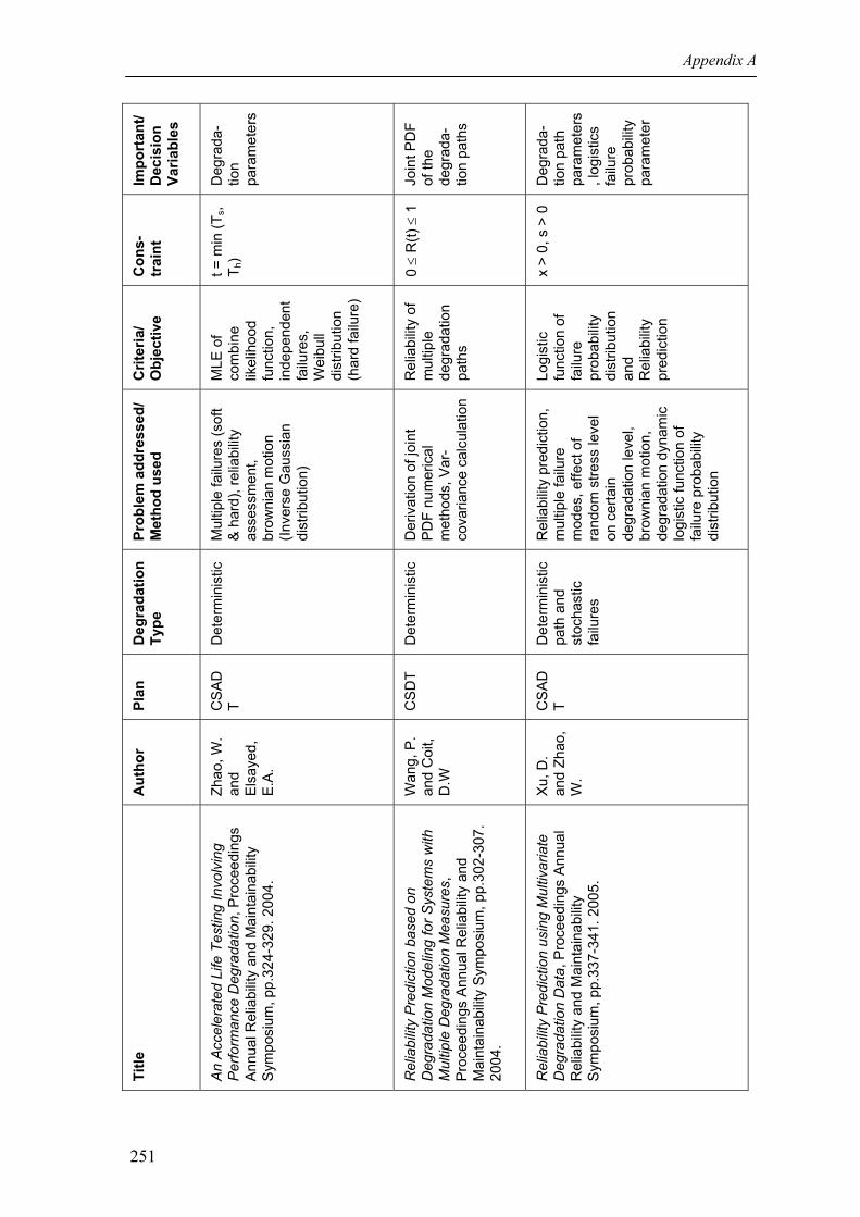
Appendix A
Impo
rtan
t/ D
ecis
ion
Varia
bles
Deg
rada
-tio
n pa
ram
eter
s
Join
t PD
F of
the
degr
ada-
tion
path
s
Deg
rada
-tio
n pa
th
para
met
ers
, log
istic
s fa
ilure
pr
obab
ility
pa
ram
eter
Con
s-tr
aint
t = m
in (T
s, T h
)
0 ≤
R(t)
≤ 1
x >
0, s
> 0
Crit
eria
/ O
bjec
tive
MLE
of
com
bine
lik
elih
ood
func
tion,
in
depe
nden
t fa
ilure
s,
Wei
bull
dist
ribut
ion
(har
d fa
ilure
)
Rel
iabi
lity
of
mul
tiple
de
grad
atio
n pa
ths
Logi
stic
fu
nctio
n of
fa
ilure
pr
obab
ility
di
strib
utio
n an
d R
elia
bilit
y pr
edic
tion
Prob
lem
add
ress
ed/
Met
hod
used
Mul
tiple
failu
res
(sof
t &
har
d), r
elia
bilit
y as
sess
men
t, br
owni
an m
otio
n (In
vers
e G
auss
ian
dist
ribut
ion)
Der
ivat
ion
of jo
int
PD
F nu
mer
ical
m
etho
ds, V
ar-
cova
rianc
e ca
lcul
atio
n
Rel
iabi
lity
pred
ictio
n,
mul
tiple
failu
re
mod
es, e
ffect
of
rand
om s
tress
leve
l on
cer
tain
de
grad
atio
n le
vel,
brow
nian
mot
ion,
de
grad
atio
n dy
nam
ic
logi
stic
func
tion
of
failu
re p
roba
bilit
y di
strib
utio
n
Deg
rada
tion
Type
Det
erm
inis
tic
Det
erm
inis
tic
Det
erm
inis
tic
path
and
st
ocha
stic
fa
ilure
s
Plan
CS
AD
T CS
DT
CS
AD
T
Aut
hor
Zhao
, W.
and
Els
ayed
, E.
A.
Wan
g, P
. an
d C
oit,
D.W
Xu,
D.
and
Zhao
, W
.
Title
An
Acc
eler
ated
Life
Tes
ting
Invo
lvin
g P
erfo
rman
ce D
egra
datio
n, P
roce
edin
gs
Ann
ual R
elia
bilit
y an
d M
aint
aina
bilit
y S
ympo
sium
, pp.
324-
329.
200
4.
Rel
iabi
lity
Pre
dict
ion
base
d on
D
egra
datio
n M
odel
ing
for S
yste
ms
with
M
ultip
le D
egra
datio
n M
easu
res,
P
roce
edin
gs A
nnua
l Rel
iabi
lity
and
Mai
ntai
nabi
lity
Sym
posi
um, p
p.30
2-30
7.
2004
.
Rel
iabi
lity
Pre
dict
ion
usin
g M
ultiv
aria
te
Deg
rada
tion
Dat
a, P
roce
edin
gs A
nnua
l R
elia
bilit
y an
d M
aint
aina
bilit
y S
ympo
sium
, pp.
337-
341.
200
5.
251

Appendix B
Multivariate Degradation Model Simulation
In order to make an example from generated data, a simulation procedure to generate multivariate
degradation data is needed. For a bivariate random variable data, the simplest data generation
procedure is by utilizing conditional distribution, as:
1. generate u1 and v from U(0,1)
2. generate Y(1) from F(1) using u1
3. generate u2 from the conditional distribution with ( )ρ;12 UUc = v
4. generate Y(2) from u2 and conditional distribution in step 3.
Using the above algorithm, we only need one derivative to generate bivariate random variable.
The question is how to generate data for multivariate degradation random variable given the
marginal distributions and copula function. The copula functions that will be used here are the
copulas presented in the previous sub-chapters.
To answer this question, some modification from the generic bivariate/multivariate simulation
procedure is needed because in our case the random variables have at least two aspects that need
to be taken care of, which are the correlation between observations of a sample and correlation
between PCs of a sample. In the following sections, simulation procedures for multivariate
elliptical copulas and one-exchangeable multivariate Archimedean copulas will be presented.
B.1. Simulation Procedure for Multivariate Elliptical Copula
Assume that the marginal distributions (F(1)(y(1)), ..., F(p)(y(p))) of the random variables are known
or have been defined. Assume that the copula function is known to be multivariate Gaussian
copula (MGC) or multivariate Student-t copula, so the joint distribution of the random variables at
time t can be written respectively as:
252

Appendix B
R(t) = Φ{Φ-1(F(1)(y(1)|t)), Φ-1(F(2)(y(2)|t)), . . . , Φ-1(F(p)(y(p)|t))}
Or
R(t) = Tυ(tυ-1(F(1)(y(1)|t)), tυ-1(F(2)(y(2)|t))..., tυ-1(F(p)(y(p)|t))) (B.1)
Where Φ is the cumulative standard normal distribution function, Tυ is the cumulative Student-t
distribution function, and there are k = 1,...,p random variables (PCs).
Based on the definition and structure of the multivariate elliptical copulas (i.e. MGC and
multivariate Student-t copula), two simulation algorithms are proposed to generate multivariate
degradation data based. The first procedure uses conditional probability principle. Meanwhile,
the second algorithm is based on the simulation idea presented in the book of Law and Kelton
(2000) page 480 for generating multivariate normal random variables.
For the first simulation procedure, a modification of the classic procedure is needed for the
reasons mentioned. It can be describes as:
1. Generate u(1), v(2), v(3), ..., v(p) from U(0,1)
2. Generate u(2) from the conditional probability copula with ( )R;)1()2( uuc = φ(Φ-1(v(2)))
3. Generate u(p) from the conditional distribution with ( )R;,, )1(1)( −pp uuuc K = φ(Φ-1(v(p))),
4. Repeat step 1-3 for all samples and all measurement times. We will get p matrices of
probability values with the rows correspond to the sample no. and the columns correspond to
the measurement times.
5. With assumption that all samples have the same variance matrix, calculate the lower
triangular matrix (CL) which can be calculated from: CL × CU = Vi using Cholesky
decomposition.
6. Generate the data of the kth performance characteristic of ith sample at jth measurement time as:
253

Appendix B
)(kijY = + , where is the component of CL and is the component of
probability matrix generated in step 1-4.
)(kijμ ∑
=
n
j
kijjj uc
1
)(
*** . *jjc )(
*k
iju
For example, the MGC conditional probability copula that is used can be written as the following
equation:
( )R;,, )1()1()( −pp uuuc K
= [ ]( )( ) ( )( ) ( ) 2
111
2)(11
1
21
11
)(1
11
5.0exp −−−
−−−
−−
−⎪⎭
⎪⎬⎫
⎪⎩
⎪⎨⎧
⎥⎥⎦
⎤
⎢⎢⎣
⎡Φ−
−
−Φ− rRr
rRrζRr T
pTp
pT
p-p-
p
uu (B.2)
The following definition is needed for the calculation of (B.2).
⎥⎦
⎤⎢⎣
⎡=
11
rrR
R p- and r = (r1p, …, r(p-1)p)T
ζ = (ζp-1, ζp) with ζk = Φ-1(u(k))
The second algorithm proposed is the modification of the algorithm proposed in the paper of
Embrechts et.al. (2001). The algorithm proposed in their paper, is mainly for one event.
However, in our case, the data consists of series of observations of PCs taken in more than one
measurement time. Therefore, with some modification, the second simulation algorithm is
obtained as follows,
1. Define matrix R, which is the product-moment correlation matrix of between PCs
correlations. This matrix can be obtained from matrix R* (matrix of measure of association),
2. Calculate the lower triangular matrix (AL) of R using Cholesky decomposition,
3. With the knowledge of the variance function and working correlation matrix of between
observations in a sample, find the lower triangular matrix (CL) which can be calculated from:
254

Appendix B
CL × CU = Vi using Cholesky decomposition. Assume that all samples have the same variance
matrix,
4. Generate )(kiju from U(0,1) with i = 1,..., m; j = 1,...,n; and k = 1,...,p,
5. Generate the data of the kth performance characteristic of ith sample at jth measurement time
as:
)(kijY = + + , where is the component of CL, is
the component of AL, and is the component of probability matrix generated in step 3.
)(kijμ ∑
=
k
k
kij
kjjkk
uca1
)()(
*
*
* .. ∑−
=
1
1
)(
*** .
j
j
kijjj uc *jjc *kk
a
)(*k
iju
The above two simulation procedure will provide the generated multivariate degradation data
observation. The generated data can then be used in demonstrating a defined multivariate
degradation problem based on MGC assumption for the dependence structure. The first algorithm
can also be used to generate multivariate degradation data from other copulas family. Meanwhile,
the second algorithm provides a simple procedure for Elliptical copulas.
B.2. Simulation Procedure for Multivariate Archimedean Copula
Simulation procedures for generating data from given Archimedean copula and marginal
distributions have been proposed and discussed by some authors such as: Genest (1987), Lee
(1993), Embrechts et.al. (2001), Whelan (2004), and Wu et.al. (2006). However, these simulation
procedures are mostly for generating one set of bivariate or multivariate data and not for
generating data which also has serial correlation. Therefore, some adjustment of the simulation
procedure is needed.
For generating multivariate degradation data from a multivariate Archimedean copula with one-
exchangeable parameter and certain defined marginal degradation distribution functions the first
algorithm presented in section A.1 can also be used.
255

Appendix B
Besides the first simulation procedure in A.1, another simulation algorithm for exchangeable
multivariate Archimedean copula is discussed by Wu et.al. (2006). However, since this algorithm
is not intended to generate multivariate degradation data with possible serial correlation, some
manipulation/modification of the algorithm is needed. The modified algorithm is:
1. Generate )(kijw independent U(0,1) random variables with i = 1,..., m; j = 1,...,n; and k = 1,...,p
2. For k = 1, 2,..., p-1, set )(kijs = ( ) kk
ijw1)(
3. Set l = ( ) ⎟⎠⎞⎜
⎝⎛− kk
ijL wF1)(1
4. Set )1(iju = ( )( )lss p
ijij ρρ )1()1(1 −− L , )( piju = ( ) ( )( )ls p
ij ρρ )1(1 1 −− − , and for k = 2,..., p-1 set )(kiju =
( ) ( )( )lsij ρ)( *
s p
kkk
ijρ ∏ −
=−− −
1
1)1(1
*1
5. With the knowledge of the variance function and working correlation matrix of between
observations in a sample, find the lower triangular matrix (CL) which can be calculated from:
CL × CU = Vi using Cholesky decomposition. This is done with assumption that all samples
have the same variance matrix.
7. Generate the data of the kth performance characteristic of ith sample at jth measurement time as:
)(kijY = )(k
ijμ + , where *jjc is the component of CL. ∑=
n
j
kijjj uc
1
)(
*** .
In order to use the above modified algorithm, the multivariate Archimedean copula, marginal
distribution functions, marginal degradation variance functions and their working correlation
matrix are need to be defined. Besides these, the following equations are also needed:
(l) = LF ( ) ( )( ) ( )[ ]∑ −
=−−×
1
0)(11
!1p
kkkk ll
kρρρ = ( ) ( )( ) ( )[ ]∑ −
=−−×+
1
1)(11
!1p
kkkk ll
kl ρρρ (B.3)
With is the kth derivative of the inverse of the Archimedean copula generator. )(1 k−ρ
256

Appendix C –Listings of Some Matlab ™ Functions
Some Matlab ™ functions (in .m-files) have been written to facilitate the calculation of
the proposed bivariate and multivariate reliability models. The listings of the functions
are presented in this appendix. At each m-file, an explanation about the function is given
in the beginning of the function.
Copulabisurvival2 function copulabisurvival2 %COPULABISURVIVAL2 %This function computes the joint survival distribution %of bivariate Performance Characteristic Degradation data %the marginal distributions are continuous distributions %of the marginal Time-to-Failure with t>= 0 for %Bivariate CSDT Model 1 fprintf('\n') %This is the part that requires the user's input on the marginal distribution disp('The Available marginal distributions are:') disp('1. Normal distribution') disp('2. Log Normal distribution') disp('3. Exponential distribution') disp('4. Weibull distribution') dist1 = input('\nThe marginal TTF distribution of the first PC is (1-4): '); while (dist1 < 1) || (dist1 > 4) dist1 = input('The first marginal TTF distribution must be in (1-4):'); end dist2 = input('\nThe marginal TTF distribution of the second PC is (1-4): '); while (dist2 < 1) || (dist2 > 4) dist2 = input('The second marginal TTF distribution must be in (1-4):'); end fprintf('\n')%This is the input part for the Copula choice disp('The Available copula functions are:') disp('1. Gaussian') disp('2. Frank') Copula = input('The chosen copula function is [1 - 2]: '); while (Copula < 1) || (Copula > 2) Copula = input('The Copula function must be in (1-2):'); end fprintf('\n') disp('Summary of input:') fprintf('\nThe first marginal distribution is %1.0f ', dist1) fprintf('\nThe second marginal distribution is %1.0f ', dist2) fprintf('\nThe copula function to be used is %1.0f \n ', Copula)
257

Appendix C
fprintf('\n')%This is the input of the (predicted) failure times of both failure mechanism %The input data must be entered according to the sample no order m = input('\How many samples are available?'); fprintf('\nTTF data of the first Failure Characteristic are:\n') ttf1 = ttfinput(m); fprintf('\nTTF data of the second Failure Characteristic are:\n') ttf2 = ttfinput(m); tau = kendall(ttf1, ttf2); tlast = input('\nThe last survival probability plotting time is: '); tstep = input('\nThe time increment step is: '); trange = (0:tstep:tlast)'; fprintf('\nThe parameter(s) of the first marginal distribution is(are):\n') [cdf1,pdf1] = marginal(dist1,trange); sur1 = 1.-cdf1; fprintf('\nThe parameter(s) of the second marginal distribution is(are):\n') [cdf2,pdf2] = marginal(dist2,trange); sur2 = 1.-cdf2; fprintf('\nThe Kendall tau correlation is: %1.4f',tau) switch Copula case 1 if tau == 1%this is the modification for copulaparam.m when the correlation is almost perfect tau = 0.9999999; end if tau == -1 tau = -0.9999999; end rho = copulaparam('Gaussian', tau); jointpdf = copulapdf('Gaussian', [cdf1 cdf2], rho); jointsur = sur1 + sur2 - 1 + copulacdf('Gaussian', [cdf1 cdf2], rho); subplot(2,2,1); plot(trange,pdf1) xlabel('Time') ylabel('PDF 1st Data') title('PDF of first failure mechanism') subplot(2,2,2); plot(trange,pdf2) xlabel('Time') ylabel('PDF 2nd Data') title('PDF of second failure mechanism') subplot(2,2,3); plot(trange,jointpdf) xlabel('Time') ylabel('Joint PDF') title('Joint PDF of the product (TTF)') subplot(2,2,4); plot(trange,jointsur) xlabel('Time') ylabel('Survival Probability') title('Joint Survival Probability') %This additional line is to write the joint S into Excel File %xlswrite('tempdata.xls', [trange surdata], 'Survival
258

Appendix C
Probability', 'A2'); case 2 alpha = copulaparam('Frank',tau); jointpdf = copulapdf('Frank', [cdf1 cdf2], alpha); jointsur = sur1 + sur2 - 1 + copulacdf('Frank',[cdf1 cdf2],alpha); subplot(2,2,1); plot(trange,pdf1) xlabel('Time') ylabel('PDF 1st Data') title('PDF of first failure mechanism') subplot(2,2,2); plot(trange,pdf2) xlabel('Time') ylabel('PDF 2nd Data') title('PDF of second failure mechanism') subplot(2,2,3); plot(trange,jointpdf) xlabel('Time') ylabel('Joint PDF') title('Joint PDF of the product (TTF)') subplot(2,2,4); plot(trange,jointsur) xlabel('Time') ylabel('Survival Probability') title('Joint Survival Probability') end function ttf = ttfinput(m) %TTFINPUT(m) stores the (predicted) TTF data of a Failure Characteristic %The data is stored as a column vector ttf = zeros(m,1); for i = 1:m fprintf('\nTTF no- %1.0f ',i) ttf(i)= input('is:'); end ttf(:,1); end function [ttfcdf,ttfpdf] = marginal(dist, t) %MARGINAL Array of Marginal CDF and PDF %this function calculate the CDF of the time-to-failure of the %each marginal PC %the inputs (dist,t) where dist = the marginal distribution type %and t = vector of measurement times m = length(t); ttfcdf = zeros(m,1); ttfpdf = zeros(m,1); switch dist case 1 Mu = input('Value of MU (mean) is: '); Sigma = input('Value of Sigma (std deviation) is: '); for i = 1:m ttfcdf(i,1) = normcdf(t(i,1),Mu,Sigma); ttfpdf(i,1) = normpdf(t(i,1),Mu,Sigma); end case 2 Mu = input('Value of log MU (log mean) is: ');
259

Appendix C
Sigma = input('Value of log Sigma (log std deviation) is: '); for i = 1:m ttfcdf(i,1) = logncdf(t(i,1),Mu,Sigma); ttfpdf(i,1) = lognpdf(t(i,1),Mu,Sigma); end case 3 Mu = input('Value of location parameter Mu is: '); for i = 1:m ttfcdf(i,1) = expcdf(t(i,1),Mu); ttfpdf(i,1) = exppdf(t(i,1),Mu); end case 4 Alpha = input('Value of scale parameter alpha is: '); Beta = input('Value of shape parameter beta is: '); for i = 1:m ttfcdf(i,1) = wblcdf(t(i,1),Alpha,Beta); ttfpdf(i,1) = wblpdf(t(i,1),Alpha,Beta); end otherwise disp('Error in distribution input') end [ttfcdf(:,1),ttfpdf(:,1)]; end end function tau = kendall(x,y) %KENDALL Kendall's rank correlation coefficient. % TAU = KENDALL(X) returns a matrix TAU of pairwise Kendall's rank % correlation coefficients between columns of the matrix X. % % TAU = KENDALL(X,Y) returns Kendall's rank correlation coefficient TAU % between the vectors X and Y. % Written by Peter Perkins, The MathWorks, Inc. % Revision: 1.0 Date: 2003/09/05 % This function is not supported by The MathWorks, Inc. % % Requires MATLAB R13. if nargin == 1 [n,p] = size(x); tau = eye(p); for row = 1:(p-1) for col = (row+1):p s = 0; for i = 1:n s = s + sum(sign(x(i:n,row)-x(i,row)).*sign(x(i:n,col)-x(i,col))); end tau(row,col) = s .* 2./(n.*(n-1)); tau(col,row) = tau(row,col); end end else if ~((ndims(x) == 2) && any(size(x) == 1)) || ... ~((ndims(y) == 2) && any(size(y) == 1)) || (numel(x) ~= numel(y))
260

Appendix C
error('X and Y must be vectors of the same length.'); end n = numel(x); tau = 0; for i = 1:n tau = tau + sum(sign(x(i:n)-x(i)).*sign(y(i:n)-y(i))); end tau = tau .* 2./(n.*(n-1)); end end
Frankpdfadjmodel1 function frankpdfadjmodel1 %FRANKPDFADJMODEL1 %this function is to adjust the Bivariate Frank copula PDF %to get the correct estimated bivariate Frank copula PDF adjusted %to the time line for model 1 where the marginal is TTF distribution %with marginal PDF of the PC follow standard distribution fprintf('\n') tlast = input('\nThe max expected life of the product is: '); fprintf('\n') %This is the part that requires the user's input on the marginal distribution disp('The Available marginal distributions are:') disp('1. Normal distribution') disp('2. Log Normal distribution') disp('3. Exponential distribution') disp('4. Weibull distribution') disp('5. Inverse Gaussian') disp('6. Birnbaum Saunders') disp('7. Gamma') dist1 = input('\nThe marginal TTF distribution of the first PC is (1-7): '); while (dist1 < 1) || (dist1 > 7) dist1 = input('The first marginal TTF distribution must be in (1-7):'); end dist2 = input('\nThe marginal TTF distribution of the second PC is (1-7): '); while (dist2 < 1) || (dist2 > 7) dist2 = input('The second marginal TTF distribution must be in (1-7):'); end %Calculation of the 1st PC PDF %using the choosen marginal distribution tstep = input('\nThe time increment step of the time line is: '); m = round(tlast/tstep); k = 0; for i=1:m trange(i,1)=k; k = k+tstep; end fprintf('\nThe first marginal distribution calculation :\n')
261

Appendix C
[cdf1,pdf1] = marginal(dist1,trange); sur1 = 1.-cdf1; fprintf('\nThe second marginal distribution calculation:\n') [cdf2,pdf2] = marginal(dist2,trange); sur2 = 1.-cdf2; IntegralPDF1 = trapz(trange,pdf1); fprintf('\nThe 1st PC PDF integration is %3.8f ', IntegralPDF1) for i = 1:m PDF1adj(i,1) = pdf1(i,1); end %Calculation of the 2nd PC PDF IntegralPDF2 = trapz(trange,pdf2); fprintf('\nThe 2nd PC PDF integration is %3.8f ', IntegralPDF2) for i = 1:m PDF2adj(i,1) = pdf2(i,1); end %Calculation of the Frank copula PDF fprintf('\n') alpha = input('\nThe Frank copula parameter is: '); for i = 1:m Frankpdf(i,1) = copulapdf('Frank',[cdf1(i,1) cdf2(i,1)], alpha) * pdf1(i,1) * pdf2(i,1); Frankcdf(i,1) = copulacdf('Frank',[cdf1(i,1) cdf2(i,1)], alpha); Franksur(i,1) = copulacdf('Frank',[sur1(i,1) sur2(i,1)],alpha); end IntegralPDF = trapz(trange,Frankpdf); fprintf('\nThe joint PDF integration is %3.8f ', IntegralPDF) for i = 1:m PDFadj(i,1) = Frankpdf(i,1)/IntegralPDF; end Integralnew = trapz(trange,PDFadj); A = 't'; B = 'PDF1'; C = 'PDF2'; D = 'JointPDF'; E = 'CDF1'; F = 'CDF2'; G = 'JointCDF'; H = 'JointReliability'; A = cellstr(A); B = cellstr(B); C = cellstr(C); D = cellstr(D); E = cellstr(E); F = cellstr(F); G = cellstr(G); H = cellstr(H); fprintf('\nThe new joint PDF integration is %3.8f ', Integralnew) xlswrite('tempdata.xls', [A B C D E F G H], 'PDF data', 'A1');
262

Appendix C
xlswrite('tempdata.xls', [trange PDF1adj PDF2adj PDFadj cdf1 cdf2 Frankcdf Franksur], 'PDF data', 'A2'); function [ttfcdf,ttfpdf] = marginal(dist, trange) %MARGINAL Array of Marginal CDF and PDF %this function calculate the CDF of the time-to-failure of the %each marginal PC %the inputs (dist,t) where dist = the marginal distribution type %and trange = vector of measurement times ttfcdf = zeros(m,1); ttfpdf = zeros(m,1); switch dist case 1 Mu = input('Value of MU (mean) is: '); Sigma = input('Value of Sigma (std deviation) is: '); for i = 1:m ttfcdf(i,1) = normcdf(trange(i,1),Mu,Sigma); ttfpdf(i,1) = normpdf(trange(i,1),Mu,Sigma); end case 2 Mu = input('Value of log MU (log mean) is: '); Sigma = input('Value of log Sigma (log std deviation) is: '); ttfcdf(1,1) = 0; ttfpdf(1,1)= 0; for i = 2:m ttfcdf(i,1) = logncdf(trange(i,1),Mu,Sigma); ttfpdf(i,1) = lognpdf(trange(i,1),Mu,Sigma); end case 3 Mu = input('Value of location parameter Mu is: '); for i = 1:m ttfcdf(i,1) = expcdf(trange(i,1),Mu); ttfpdf(i,1) = exppdf(trange(i,1),Mu); end case 4 Alpha = input('Value of scale parameter alpha is: '); Beta = input('Value of shape parameter beta is: '); for i = 1:m ttfcdf(i,1) = wblcdf(trange(i,1),Alpha,Beta); ttfpdf(i,1) = wblpdf(trange(i,1),Alpha,Beta); end case 5 Mu = input('Value of the parameter Mu is: '); L = input('Value of the parameter Lambda is: '); ttfcdf(1,1) = 0; ttfpdf(1,1) = 0; for i= 2:m ttfcdf(i,1) = cdf('inversegaussian',trange(i,1),Mu,L); ttfpdf(i,1) = pdf('inversegaussian',trange(i,1),Mu,L); end case 6 Beta = input('Value of the parameter Beta is: '); Gamma = input('Value of the parameter Gamma is: '); for i= 1:m ttfcdf(i,1) = cdf('birnbaumsaunders',trange(i,1),Beta,Gamma);
263

Appendix C
ttfpdf(i,1) = pdf('birnbaumsaunders',trange(i,1),Beta,Gamma); end case 7 Alpha = input('Value of the shape parameter is: '); Beta = input('Value of the scale parameter is: '); for i= 1:m ttfcdf(i,1) = cdf('gamma',trange(i,1),Alpha, Beta); ttfpdf(i,1) = pdf('gamma',trange(i,1),Alpha, Beta); end otherwise disp('Error in distribution input') end [ttfcdf(:,1),ttfpdf(:,1)]; end end
Bivariatemod2 function bivariatemod2 %BIVARIATEMOD2 %This function computes the joint survival distribution %of bivariate Performance Characteristic Degradation data %the marginal distributions are continuous distributions %of the degradation data and follow simple linear function %This will calculate the marginal and system reliability %including the adjusted PDF according to MODEL 2 of %the thesis of Josephine fprintf('\n') %This is the part that requires the user's input on the marginal distribution disp('The Available marginal distributions are:') disp('1. Normal distribution') disp('2. Log Normal distribution') disp('3. Exponential distribution') disp('4. Weibull distribution') disp('5. Gamma distribution') disp('6. Inverse Gaussian (a) distribution') %This is for lambda = (A*t)^2 disp('7. Inverse Gaussian (b) distribution') %This is for lambda = A+B*t+C*t^2 dist1 = input('\nThe marginal distribution of the first PC is (1-7): '); while (dist1 < 1) || (dist1 > 7) dist1 = input('The first marginal distribution must be in (1-7):'); end dist2 = input('\nThe marginal distribution of the second PC is (1-7): '); while (dist2 < 1) || (dist2 > 7) dist2 = input('The second marginal distribution must be in (1-7):'); end fprintf('\n')%This is the input part for the Copula choice disp('The Available copula functions are:') disp('1. Gaussian')
264

Appendix C
disp('2. Frank') Copula = input('The chosen copula function is [1 - 2]: '); while (Copula < 1) || (Copula > 2) Copula = input('The Copula function must be in (1-2):'); end fprintf('\n') disp('Summary of input:') fprintf('\nThe first marginal distribution is %1.0f ', dist1) fprintf('\nThe second marginal distribution is %1.0f ', dist2) fprintf('\nThe copula function to be used is %1.0f \n ', Copula) fprintf('\n') %This is the input of the time range tlast = input('\nThe max expected life of the product is: '); tstep = input('\nThe time increment step of the time line is: '); m = round(tlast/tstep); k = 0; for i=1:m trange(i,1)=k; k = k+tstep; end fprintf('\nThe parameter(s) of the first marginal distribution is(are):\n') [cdf1,pdf1] = marginal(dist1); fprintf('\nThe parameter(s) of the second marginal distribution is(are):\n') [cdf2,pdf2] = marginal(dist2); %PDF adjustment of the first PC IntegralPDF1 = trapz(trange,pdf1); fprintf('\nThe 1st PC PDF integration is %3.8f ', IntegralPDF1) for i = 1:m pdf1adj(i,1) = pdf1(i,1)/IntegralPDF1; end %PDF adjustment of the second PC IntegralPDF2 = trapz(trange,pdf2); fprintf('\nThe 2nd PC PDF integration is %3.8f ', IntegralPDF2) for i = 1:m pdf2adj(i,1) = pdf2(i,1)/IntegralPDF2; end switch Copula case 1 rho = input('\nThe Gaussian copula parameter is: '); copulapdf('Gaussian', [cdf1 cdf2], rho); for i = 1:m jointpdf (i,1) = copulapdf('Gaussian', [cdf1(i,1) cdf2(i,1)], rho)*pdf1adj(i,1)*pdf2adj(i,1); end IntegralPDF = trapz(trange,jointpdf); fprintf('\nThe joint PDF integration is %3.10e ', IntegralPDF)
265

Appendix C
for i = 1:m jointpdfadj(i,1) = jointpdf(i,1)/IntegralPDF; end jointsur = copulacdf('Gaussian', [cdf1 cdf2], rho); subplot(2,2,1); plot(trange,pdf1adj) xlabel('Time') ylabel('PDF 1st Data') title('PDF of first failure mechanism') subplot(2,2,2); plot(trange,pdf2adj) xlabel('Time') ylabel('PDF 2nd Data') title('PDF of second failure mechanism') subplot(2,2,3); plot(trange,jointpdfadj) xlabel('Time') ylabel('Joint PDF') title('Joint PDF of the product (TTF)') subplot(2,2,4); plot(trange,jointsur) xlabel('Time') ylabel('Survival Probability') title('Joint Survival Probability') %This additional line is to write the joint S into Excel File %xlswrite('tempdata.xls', [trange surdata], 'Survival Probability', 'A2'); case 2 alpha = input('\nThe Frank copula parameter is: '); for i = 1:m jointpdf (i,1) = copulapdf('Frank', [cdf1(i,1) cdf2(i,1)], alpha)*pdf1adj(i,1)*pdf2adj(i,1); end IntegralPDF = trapz(trange,jointpdf); fprintf('\nThe joint PDF integration is %3.10e ', IntegralPDF) for i = 1:m jointpdfadj(i,1) = jointpdf(i,1)/IntegralPDF; end jointsur = copulacdf('Frank',[cdf1 cdf2],alpha); subplot(2,2,1); plot(trange,pdf1adj) xlabel('Time') ylabel('PDF 1st Data') title('PDF of first failure mechanism') subplot(2,2,2); plot(trange,pdf2adj) xlabel('Time') ylabel('PDF 2nd Data') title('PDF of second failure mechanism') subplot(2,2,3); plot(trange,jointpdfadj) xlabel('Time') ylabel('Joint PDF') title('Joint PDF of the product (TTF)') subplot(2,2,4); plot(trange,jointsur) xlabel('Time') ylabel('Survival Probability') title('Joint Survival Probability') end
266

Appendix C
%fprintf('\nThe joint survival data is:\n') %jointsur function [ttfcdf,ttfpdf] = marginal(dist) %MARGINAL Array of Marginal CDF and PDF %this function calculate the CDF of the time-to-failure of the %each marginal PC %the inputs (dist,t) where dist = the marginal distribution type %and t = vector of measurement times ttfcdf = zeros(m,1); ttfpdf = zeros(m,1); k = 0; switch dist case 1 Ma = input('\The intersection of the mean parameter of the PC is: '); Mb = input('\The slope of the mean of the PC is: '); Sigma = input('Value of Sigma (std deviation) is: '); c = input('\The threshold value of PC is: '); for i = 1:m M(i,1) = Ma + Mb*k; ttfcdf(i,1) = normcdf(c,M(i,1),Sigma); ttfpdf(i,1) = normpdf(c,M(i,1),Sigma); k = k + tstep; end case 2 Ma = input('\The intersection of the mean parameter of the PC is: '); Mb = input('\The slope of the mean of the PC is: '); Sigma = input('Value of Sigma (std deviation) is: '); c = input('\The threshold value of PC is: '); ttfcdf(1,1) = 1; ttfpdf(1,1)= 0; k = k + tstep; for i = 2:m M(i,1) = Ma + Mb*k; ttfcdf(i,1) = logncdf(c,M(i,1),Sigma); ttfpdf(i,1) = lognpdf(c,M(i,1),Sigma); k = k + tstep; end case 3 Ma = input('\The intersection of location parameter Mu is: '); Mb = input('\The slope of the location parameter of the PC is: '); c = input('\The threshold value of PC is: '); ttfcdf(1,1) = 1; ttfpdf(1,1)= 0; k = k + tstep; for i = 2:m M(i,1) = Ma + Mb*k; ttfcdf(i,1) = expcdf(c,M(i,1)); ttfpdf(i,1) = exppdf(c,M(i,1)); k = k + tstep; end case 4 A1 = input('The intersection of scale parameter alpha is: ');
267

Appendix C
A2 = input('\The slope of the scale parameter alpha is: '); Beta = input('\Value of shape parameter beta is: '); c = input('\The threshold value of PC is: '); if A1==0 ttfcdf(1,1) = 1; ttfpdf(1,1)= 0; k = k + tstep; for i = 2:m Alpha(i,1) = A1 + A2*k; ttfcdf(i,1) = wblcdf(c,Alpha(i,1),Beta); ttfpdf(i,1) = wblpdf(c,Alpha(i,1),Beta); k = k + tstep; end else for i = 1:m Alpha(i,1) = A1 + A2*k; ttfcdf(i,1) = wblcdf(c,Alpha(i,1),Beta); ttfpdf(i,1) = wblpdf(c,Alpha(i,1),Beta); k = k + tstep; end end case 5 %This is only for the fatigue-crack bivariate example model 3 SD = input('\The standard deviation of the PC is: '); disp('Other components of parameter beta of the PC is: ') A1 = input('\The intersection of the X.b is: '); A2 = input('\The slope of the X.b is: '); c = input('\The threshold value of the PC is: '); alpha = 1/(SD^2); for i = 1:m mu(i,1) = 90/(100 - (A1 + A2*k)); beta(i,1) = (SD*SD)* mu(i,1); if beta(i,1) < 0 ttfcdf(i,1) = 0; ttfpdf(i,1) = 0; else ttfcdf(i,1) = gamcdf(c, alpha, beta(i,1)); ttfpdf(i,1) = gampdf(c, alpha, beta(i,1)); end k = k + tstep; end case 6 %This is only for Yiu Man data model 2 Inverse Gaus Ma = input('\The intersection of the mu parameter of the PC is: '); Mb = input('\The slope of the mu of the PC is: '); La = input('\The parameter of the Lambda parameter regression of the PC is: '); c = input('\The threshold value of PC is: '); k = tstep; ttfcdf(1,1) = 1; ttfpdf(1,1) = 0; for i = 2:m M(i,1) = Ma + Mb*k; L(i,1) = (La *(k))^2; if cdf('inversegaussian', c, M(i,1), L(i,1))> 0 ttfcdf(i,1) = cdf('inversegaussian', c,M(i,1),L(i,1)); ttfpdf(i,1) = pdf('inversegaussian',
268

Appendix C
c,M(i,1),L(i,1)); else ttfcdf(i,1)= 0; ttdpdf(i,1)= 0; end k = k + tstep; end case 7 %This is only for Yiu Man data model 2 Inverse Gaus PC 2 Ma = input('\The intersection of the mu parameter of the PC is: '); Mb = input('\The slope of the mu of the PC is: '); La = input('\The intersection of the Lambda parameter of the PC is: '); Lb = input('\The 2-nd parameter of the Lambda parameter of the PC is: '); Lc = input('\The 3-rd parameter of the Lambda parameter of the PC is: '); c = input('\The threshold value of PC is: '); for i = 1:m M(i,1) = Ma + Mb*k; L(i,1) = exp(La + Lb*(k)+Lc*k^2); ttfcdf(i,1) = cdf('inversegaussian', c,M(i,1),L(i,1)); ttfpdf(i,1) = pdf('inversegaussian', c,M(i,1),L(i,1)); k = k + tstep; end otherwise disp('Error in distribution input') end [ttfcdf(:,1),ttfpdf(:,1)]; end %PDF adjustment of joint pdf Integralnew = trapz(trange,jointpdfadj); fprintf('\nThe new joint PDF integration is %3.10e ', Integralnew) %writing the data into Excel(TM) file A = ['t']; B = ['PDF1']; C = ['PDF2']; D = ['JointPDF']; E = ['R1']; F = ['R2']; G = ['JointRel']; A = cellstr(A); B = cellstr(B); C = cellstr(C); D = cellstr(D); E = cellstr(E); F = cellstr(F); G = cellstr(G); xlswrite('tempdata.xls', [A B C D E F G], 'Summary', 'A1'); xlswrite('tempdata.xls', [trange pdf1adj pdf2adj jointpdfadj cdf1 cdf2 jointsur], 'Summary', 'A2'); end
269

Appendix C
Multifrankpdfadjmodel1 function multifrankpdfadjmodel1 %MULTIFRANKPDFADJMODEL1 %this function is to adjust the Frank copula PDF %to get the correct multivariate Frank copula PDF adjusted %to the time line for model 1 where the marginal is TTF distribution %with marginal PDF of the PC follow standard distribution %and this is for 4PC variate data fprintf('\n') tlast = input('\nThe max expected life of the 4variate degraded product is: '); fprintf('\n') %This is the part that requires the user's input on the marginal distribution disp('The Available marginal distributions are:') disp('1. Normal distribution') disp('2. Log Normal distribution') disp('3. Exponential distribution') disp('4. Weibull distribution') disp('5. Inverse Gaussian') disp('6. Birnbaum Saunders') dist1 = input('\nThe marginal TTF distribution of the first PC is (1-6): '); while (dist1 < 1) || (dist1 > 6) dist1 = input('The first TTF marginal distribution must be in (1-6):'); end dist2 = input('\nThe marginal TTF distribution of the second PC is (1-6): '); while (dist2 < 1) || (dist2 > 6) dist2 = input('The second TTF marginal distribution must be in (1-6):'); end dist3 = input('\nThe marginal TTF distribution of the third PC is (1-6): '); while (dist3 < 1) || (dist3 > 6) dist3 = input('The third TTF marginal distribution must be in (1-6):'); end dist4 = input('\nThe marginal TTF distribution of the fourth PC is (1-6): '); while (dist4 < 1) || (dist4 > 6) dist4 = input('The fourth TTF marginal distribution must be in (1-6):'); end %Calculation of the first marginal PC PDF %using the choosen marginal distribution tstep = input('\nThe time increment step of the time line is: '); m = round(tlast/tstep); k = 0; for i = 1:m trange(i,1)=k; k = k+tstep; end
270

Appendix C
fprintf('\nThe first marginal distribution calculation :\n') [cdf1,pdf1] = marginal(dist1,trange); sur1 = 1.-cdf1; fprintf('\nThe second marginal distribution calculation:\n') [cdf2,pdf2] = marginal(dist2,trange); sur2 = 1.-cdf2; fprintf('\nThe third marginal distribution calculation:\n') [cdf3,pdf3] = marginal(dist3,trange); sur3 = 1.-cdf3; fprintf('\nThe fourth marginal distribution calculation:\n') [cdf4,pdf4] = marginal(dist4,trange); sur4 = 1.-cdf4; IntegralPDF1 = trapz(trange,pdf1); fprintf('\nThe 1st PC PDF integration is %3.8f ', IntegralPDF1) for i = 1:m PDF1adj(i,1) = pdf1(i,1); end %Calculation of the 2nd PC PDF IntegralPDF2 = trapz(trange,pdf2); fprintf('\nThe 2nd PC PDF integration is %3.8f ', IntegralPDF2) for i = 1:m PDF2adj(i,1) = pdf2(i,1); end %Calculation of the 3rd PC PDF IntegralPDF3 = trapz(trange,pdf3); fprintf('\nThe 3rd PC PDF integration is %3.8f ', IntegralPDF3) for i = 1:m PDF3adj(i,1) = pdf3(i,1); end %Calculation of the 4th PC PDF IntegralPDF4 = trapz(trange,pdf4); fprintf('\nThe 2nd PC PDF integration is %3.8f ', IntegralPDF4) for i = 1:m PDF4adj(i,1) = pdf4(i,1); end %Calculation of the Frank copula PDF fprintf('\n') alpha = input('\nThe Frank copula parameter is: '); for i = 1:m a = -1 + exp(-alpha); b = exp(-alpha*cdf1(i,1)) * exp(-alpha*cdf2(i,1)) * exp(-alpha*cdf3(i,1)) * exp(-alpha*cdf4(i,1)); c = (exp(-alpha*cdf1(i,1))-1) * (exp(-alpha*cdf2(i,1))-1) * (exp(-alpha*cdf3(i,1))-1) * (exp(-alpha*cdf4(i,1))-1); Frankpdf(i,1) = ((-b*alpha^3/(a^3*(1+c/a^3)))+(7*alpha^3*b*c/((a^6)*(1+c/a^3)^2))-(12*alpha^3*b*c^2/((a^9)*(1+c/a^3)^3))+(6*alpha^3*b*c^3/((a^12)*(1+c/a^3)^4)))*pdf1(i,1)*pdf2(i,1)*pdf3(i,1)*pdf4(i,1); Frankcdf(i,1) = -(1/alpha)*log(1+(((exp(-alpha*cdf1(i,1))-
271

Appendix C
1)*(exp(-alpha*cdf2(i,1))-1)*(exp(-alpha*cdf3(i,1))-1)*(exp(-alpha*cdf4(i,1))-1))/(exp(-alpha)-1)^3)); Franksur(i,1) = -(1/alpha)*log(1+(((exp(-alpha*sur1(i,1))-1)*(exp(-alpha*sur2(i,1))-1)*(exp(-alpha*sur3(i,1))-1)*(exp(-alpha*sur4(i,1))-1))/(exp(-alpha)-1)^3)); end IntegralPDF = trapz(trange,Frankpdf); fprintf('\nThe joint PDF integration is %3.60e ', IntegralPDF) for i = 1:m PDFadj(i,1) = Frankpdf(i,1)/IntegralPDF; end Integralnew = trapz(trange,PDFadj); A = 't'; B = 'PDF1'; C = 'PDF2'; D = 'PDF3'; E = 'PDF4'; F = 'JointPDF'; G = 'CDF1'; H = 'CDF2'; I = 'CDF3'; J = 'CDF4'; K = 'JointCDF'; L = 'JointReliability'; A = cellstr(A); B = cellstr(B); C = cellstr(C); D = cellstr(D); E = cellstr(E); F = cellstr(F); G = cellstr(G); H = cellstr(H); I = cellstr(I); J = cellstr(J); K = cellstr(K); L = cellstr(L); fprintf('\nThe new joint PDF integration is %3.8f ', Integralnew) xlswrite('tempdata.xls', [A B C D E F G H I J K L], 'Multivariate', 'A1'); xlswrite('tempdata.xls', [trange PDF1adj PDF2adj PDF3adj PDF4adj PDFadj cdf1 cdf2 cdf3 cdf4 Frankcdf Franksur], 'Multivariate', 'A2'); function [ttfcdf,ttfpdf] = marginal(dist, trange) %MARGINAL Array of Marginal CDF and PDF %this function calculate the CDF of the time-to-failure of the %each marginal PC %the inputs (dist,t) where dist = the marginal distribution type %and trange = vector of measurement times ttfcdf = zeros(m,1); ttfpdf = zeros(m,1); switch dist case 1 Mu = input('Value of MU (mean) is: '); Sigma = input('Value of Sigma (std deviation) is: '); for i = 1:m
272

Appendix C
ttfcdf(i,1) = normcdf(trange(i,1),Mu,Sigma); ttfpdf(i,1) = normpdf(trange(i,1),Mu,Sigma); end case 2 Mu = input('Value of log MU (log mean) is: '); Sigma = input('Value of log Sigma (log std deviation) is: '); ttfcdf(1,1) = 0; ttfpdf(1,1)= 0; for i = 2:m ttfcdf(i,1) = logncdf(trange(i,1),Mu,Sigma); ttfpdf(i,1) = lognpdf(trange(i,1),Mu,Sigma); end case 3 Mu = input('Value of location parameter Mu is: '); for i = 1:m ttfcdf(i,1) = expcdf(trange(i,1),Mu); ttfpdf(i,1) = exppdf(trange(i,1),Mu); end case 4 Alpha = input('Value of scale parameter alpha is: '); Beta = input('Value of shape parameter beta is: '); for i = 1:m ttfcdf(i,1) = wblcdf(trange(i,1),Alpha,Beta); ttfpdf(i,1) = wblpdf(trange(i,1),Alpha,Beta); end case 5 Mu = input('Value of the parameter Mu is: '); L = input('Value of the parameter Lambda is: '); ttfcdf(1,1) = 0; ttfpdf(1,1) = 0; for i= 2:m ttfcdf(i,1) = cdf('inversegaussian',trange(i,1),Mu,L); ttfpdf(i,1) = pdf('inversegaussian',trange(i,1),Mu,L); end case 6 Beta = input('Value of the parameter Beta is: '); Gamma = input('Value of the parameter Gamma is: '); for i= 1:m ttfcdf(i,1) = cdf('birnbaumsaunders',trange(i,1),Beta,Gamma); ttfpdf(i,1) = pdf('birnbaumsaunders',trange(i,1),Beta,Gamma); end otherwise disp('Error in distribution input') end [ttfcdf(:,1),ttfpdf(:,1)]; end end
273


Curriculum Vitae
Josephine Kartika Sari was born in Surabaya, Indonesia, on 19th March 1976. She
received her bachelor degrees in Civil Engineering (1997) and Information Technology
(2000) from Parahyangan Catholic University and Sekolah Tinggi Teknologi Indonesia
respectively. After receiving her first bachelor degree, she started to pursue her Master
degree in Civil Engineering at Parahyangan Catholic University focusing in Soil-
Structure Interaction. At the same time, she also worked as a lecturer in Computer
Science Department at Parahyangan Catholic University. After receiving her Master
degree in 2001, she joined LCH (S), Pte. Ltd. as a consultant in marine insurance industry
until she started her PhD work within Industrial and Systems Engineering department
(National University of Singapore) and Technology Management department (Eindhoven
University of Technology). Her PhD work was supported by Centre for Design
Technology (formerly Design Technology Institute). She is currently employed with
Energy Research Centre of the Netherland and works as researcher at Knowledge-Centre
WMC. She is interested in quality and reliability modelling and analysis as well as
statistical modelling and analysis.
275


![Graphical modelling of multivariate time series · Graphical modelling of multivariate time series 237 Fig. 1 Encoding of relations XA XB [XX]by the a pairwise, b local, and c block-recursive](https://static.fdocuments.in/doc/165x107/5f9f3dbca39f3e3fad209cdf/graphical-modelling-of-multivariate-time-series-graphical-modelling-of-multivariate.jpg)