![On Stein’s method for multivariate normal approximation · Chatterjee [3], where several abstract normal approximation theorems, for approx-imating by standard Gaussian random vectors,](https://static.fdocuments.in/doc/165x107/5f53a0f2897d984734626843/on-steinas-method-for-multivariate-normal-approximation-chatterjee-3-where.jpg)
Multivariate Approximation
297
Multivariate Approximation and Applications Edited by N . D Y N Tel Aviv University D. LEVIATAN Tel Aviv University D . LEVIN Tel Aviv University A. PINKUS Technion-Israel Institute of Technology 1 CAMBRIDGE UNIVERSITY PRESS
-
Upload
alexander-golikov -
Category
Documents
-
view
246 -
download
0
Transcript of Multivariate Approximation
8/3/2019 Multivariate Approximation
http://slidepdf.com/reader/full/multivariate-approximation 1/296
Multivariate Approximationand Applications
Edited by
N. DYN
Tel Aviv University
D. LEVIATAN
Tel Aviv University
D. LEVIN
Tel Aviv U niversity
A. PINKUS
Technion-Israel Institute of Technology
1 CAMBRIDGEUNIVERSITY PRESS

8/3/2019 Multivariate Approximation
http://slidepdf.com/reader/full/multivariate-approximation 2/296
P U B L I S H E D B Y T H E P R E S S S Y N D I C A T E O F T H E U N I V E R S I T Y O F C A M B R I D G E
The Pitt Building, Trumpington Street, Cambridge, United Kingdom
C A M B R I D G E U N I V E R S I T Y P R E S SThe Edinburgh Building, Cambridge, CB2 2RU, UK40 West 20th Street, New York, NY 10011-4211, USA
10 Stamford Road, Oakleigh, VIC 3166, AustraliaRuiz de Alarcon 13, 28014 Madrid, Spain
Dock House, The Waterfront, Cape Town 8001, South Africa
http://www.canibridge.org
© Cambridge University Press 2001
This book is in copyright. Subject to statutory exceptionand to the provisions of relevant collective licensing agreements,
no reproduction of any part may take place withoutthe written permission of Cambridge University Press.
First published 2001
Printed in the United Kingdom at the University Press, Cambridge
Typeface Computer Modern 10/12pt System IATgX [UPH]
A catalogue record for this book is available from the British Library
Library of Congress Cataloguing in Publication data
ISBN 0 521 80023 4 hardback

8/3/2019 Multivariate Approximation
http://slidepdf.com/reader/full/multivariate-approximation 3/296
Contents
List of contributors Va9e v
Preface vii
1 Characterization and construction of radia l basis functions
R. Schaback and H. Wendland 1
2 Approximation and interpolation with radial functions
M.D. Buhmann 25
3 Representing and analyzing scattered da ta on spheres
H.N. M haskar, F.J. N arcowich and J.D. Ward 44
4 A survey on .^-ap proxim ation orders from shift-invariant
spaces K. Jetter and G. Plonka 73
5 Introduc tion to shift-invariant spaces. Linear independence
A. Ron 112
6 Theory and algorithms for nonuniform spline wavelets
T. Lyche, K. M0rken and E. Quak 152
7 Applied and com puta tional aspects of nonlinear wavelet
approximation A. Cohen 188
8 Subdivision, multiresolution and the construction of
scalable algorithms in computer graphics P. Schroder 213
9 M athematical methods in reverse engineering J. Hoschek 252
Index 285
m

8/3/2019 Multivariate Approximation
http://slidepdf.com/reader/full/multivariate-approximation 4/296

8/3/2019 Multivariate Approximation
http://slidepdf.com/reader/full/multivariate-approximation 5/296
Contributors
M.D. BuhmannMathematical Institute, Justus-Liebig University, 35392 Gieflen, Germanyemail: M ar tin . Buhmann8@inath. u n i- g ie s s e n . de
A. CohenLaboratoire a"Ana lyse Num erique, Universite Pierre et Marie C urie, Paris, Pranceemail: cohen@8ann. juss ieu . f r
J. HoschekDepartment of Mathematics, Darmstadt University of Technology, 64289 Darm-stadt, Germanyemail: hoschek88ma thema t ik . tu -da rms tad t .de
K. JetterInstitut fur Angew andte Mathematik und Statistik, Universitat Hohenheim, 70593Stuttgart, Germanyemail: k je t t e r89un i -hohenhe im.de
T. LycheDepartment of Informatics, University of Oslo, P.O. B ox 1080 Blindern, 0316 Oslo,Norway
email: t o m 9 8 i f i . u i o . n oH.N. MhaskarDepartment of Mathematics, California State University, Los Angeles, CA 90032,USAemail: hmhaska88ca l s ta te la . edu
K. M0rkenDepartment of Informatics, University of Oslo, P.O. Box 1080 Blindern, 0316 Oslo,Norwayemail: k n u t m 8 8 i f i . u i o . n o
F.J. NarcowichDepartment of Mathem atics, Texas A&M University, College Station, TX 77843,USAemail: fnarc88math. tamu.edu

8/3/2019 Multivariate Approximation
http://slidepdf.com/reader/full/multivariate-approximation 6/296
vi Contributors
G. Plonka
Fachbereich Mathematik, Universitdt Duisburg, 47048 Duisburg, Germany
email: plonka@@math. u n i- d u is b u rg . de
E. Quak
SINTEF Applied Mathematics, P.O. Box 124 Blindern, 0314 Oslo, Norway
email: Ew ald. QuakQSmath. s in te f . no
A. Ron
Computer Sciences Department, 1210 West Dayton, University of Wisconsin-
Madison, Madison, WI 57311, USA
email: [email protected]
R. SchabackInstitut fur Numerische und Angewandte Mathematik, Universitat Gottingen,
Lotzestrafie 16-18, 37083 Gottingen, Germany
email: schabackQQmath. u n i- g o e tt in ge n. de
P. Schroder
Department of Computer Science, California Institute of Technology, Pasadena,
CA 91125, USA
email: psS9cs.caltech.ed
J.D. Ward
Department of Mathematics, Texas A&M University, College Station, TX 77843,USA
email: [email protected]
H. Wendland
Institut fur Numerische und Angewandte Mathematik, Universitat Gottingen,
Lotzestrafie 16-18, 37083 Gottingen, Germany
email: wendland99math .uni -goet t ingen.de

8/3/2019 Multivariate Approximation
http://slidepdf.com/reader/full/multivariate-approximation 7/296
Preface
Multivariate approximation theory is today an increasingly active research
area. It deals with a multitude of problems in areas such as wavelets, multi-
dimensional splines, and radial-basis functions, and applies them, for exam-
ple, to problems in computer aided geometric design, geometric modeling,
geodesic applications and image analysis. The field is both fascinating and
intellectually stimulating since much of the mathematics of the classical
univariate theory does not straightforwardly generalize to the multivariate
setting which models many real-world problems; so new tools have had tobe, and must continue to be, developed.
This advanced introduction to multivariate approximation and related
topics consists of nine chapters written by leading experts that survey many
of the new ideas and tools and their applications. Each chapter introduces a
particular topic, takes the reader to the forefront of research and ends with
a comprehensive list of references.
This book will serve as an ideal introduction for researchers and graduate
studen ts who wish to learn abo ut the subject and see how it may be applied.
A more detailed description of each chapter follows:
Chapter 1: Characterization and construction of radial basis functions, by
R. Schaback (Gottingen) and H. Wendland (Gottingen)
This chapter introduces characterizations of (conditional) positive defi-
niteness and shows how they apply to the theory of radial basis functions.
Complete proofs of the (conditional) positive definiteness of practically all
relevant basis functions are provided. Furthermore, it is shown how some ofthese characterizations may lead to construction tools for positive definite
functions. Finally, a new construc tion technique is given which is based on
discrete methods which leads to non-radial, even non-translation invariant,
local basis functions.

8/3/2019 Multivariate Approximation
http://slidepdf.com/reader/full/multivariate-approximation 8/296
viii Preface
Chap ter 2: Approximation and interpolation with radial Junctions, by
M.D. Buhmann (Giessen)This chapter provides a short, up-to-date survey of some of the recent
developments in the research of radial basis functions. Among these new
developments are results on convergence rates of interpolation with radial
basis functions, recent contributions concerning approximation on spheres,
and computations of interpolants with Krylov space methods.
Chapter 3: Representing and analyzing scattered data on spheres, by
H.N. Mhaskar (California S tate Univ. at Los Angeles), F. J. Narcowich (Texas
A & M) and J.D. Ward (Texas A k M)Geophysical or meteorological data collected over the surface of the earth
via satellites or ground stations will invariably come from scattered sites.
There are two extremes in the problems one faces when handling such data.
The first is representing sparse data by fitting a surface to it. The second is
analyzing dense data to extract features of interest. In this chapter various
aspects of fitting surfaces to scattered data are reviewed. Analyzing data is a
more recent problem that is currently being addressed via various spherical
wavelet schemes, which are discussed along with multilevel schemes. Finallyquadrature methods, which arise in many of the wavelet schemes as well as
some interpolation methods, are touched upon.
Chapter 4: A survey on L2-approximation orders from shift-invariant
spaces, by K. Jetter (Hohenheim) and G. Plonka (Duisburg)
The aim of this chapter is to provide a self-contained introduction to
notions and results connected with the /^-approximation order of finitely
generated shift-invariant spaces. Special attention is given to the principal
shift-invariant case, where the shift-invariant space is generated from themulti-integer translates of a single generator. This case is of special interest
because of its possible applications in wavelet methods. The general finitely
generated shift-invariant space case is considered subject to a stability con-
dition being satisfied, and the recent results on so-called superfunctions are
developed. For the case of a refinable system of generators, the sum rules
for the matrix mask and the zero condition for the mask symbol, as well as
invariance properties of the associated subdivision and transfer operators,
are discussed.Chapter 5: Introduction to shift-invariant spaces. Linear independence,
by A. Ron (Madison)
Shift-invariant spaces play an increasingly important role in various areas
of mathematical analysis and its applications. They appear either implicitly
or explicitly in studies of wavelets, splines, radial basis function approxima-
tion, regular sampling, Gabor systems, uniform subdivision schemes, and

8/3/2019 Multivariate Approximation
http://slidepdf.com/reader/full/multivariate-approximation 9/296
Preface ix
perhaps in some other areas. One must keep in mind, however, that the
shift-invariant system explored in one of the above-mentioned areas might
be very different from those investigated in others . The theory of shift-
invariant spaces attempts to provide a uniform platform for all these dif-
ferent investigations. The two main pillars of that theory are the study of
th e approximation properties of shift-invariant spaces, and the study of gen-
erating sets for such spaces. Chapte r 4 had already provided an excellent
up-to-date account of the first topic. The present chapter is devoted to the
second topic, and its goal is to provide the reader with an easy and friendly
introduction to the basic principles of that topic. The core of the presenta-
tion is devoted to the study of local principal shift-invariant spaces, while
the more general cases are treated as extensions of that basic setup.
Chapter 6: Theory and algorithms for nonuniform spline wavelets, by
T. Lyche (Oslo), K. M0rken (Oslo), E. Quak (Oslo)
This chapter discusses mutually orthogonal spline wavelet spaces on non-
uniform partitions of a bounded interval, addressing the existence, unique-
ness and construction of bases of minimally supported spline wavelets. The
relevant algorithms for decomposition and reconstruction are considered as
well as some questions related to stability. In addition, a brief review is
given of the bivariate case for tensor products and arbitrary triangulations.
The chapter concludes with a discussion of some special cases.
Chapter 7: Applied and computational aspects of nonlinear wavelet app-
roximation, by A. Cohen (Paris)
Nonlinear approximation is recently being applied to computational ap-
plications such as data compression, statistical estimation and adaptive
schemes for partial differential and integral equations, especially through
the development of wavelet-based m ethods. Th e goal of this chapter is to
provide a short survey of nonlinear wavelet approximation from the per-
spective of these applications, as well as to highlight some remaining open
questions.
Chapter 8: Subdivision, multiresolution and the construction of scalable
algorithms in computer graphics, by P. Schroder (Caltech)
Multiresolution representations are a critical tool in addressing complexity
issues (time and memory) for the large scenes typically found in computer
graphics applications. Many of these techniques are based on classical sub-
division techniques and their generalizations. In this chapter we review two
exemplary applications from this area: multiresolution surface editing and
semi-regular remeshing. The former is directed towards building algorithms
which are fast enough for interactive manipulation of complex surfaces of
arbitra ry topology. The latter is concerned w ith constructing smooth pa-
8/3/2019 Multivariate Approximation
http://slidepdf.com/reader/full/multivariate-approximation 10/296
x Preface
rameterizations for arbitrary topology surfaces as they typically arise from
3D scanning techniques. Remeshing such surfaces then allows the use of
classical subdivision ideas. Th e particu lar focus here is on the practica l
aspects of making the well-understood mathematical machinery applicable
and accessible to the very general settings encountered in practice.
Chapter 9: Mathematical methods in reverse engineering, by J. Hoschek
(Darmstadt)
In many areas of industrial applications it is desirable to create a com puter
model of existing objects for which no such model is available. This pro-
cess is called reverse engineering. Reverse engineering typically starts with
digitizing an existing object. These discrete dat a must then be converted
into smooth surface models. This chapter provides a survey of the practi-
cal algorithms including triangulation, segmentation, feature lines detection,
B-spline approximation and trimming.
No book of this sort can be compiled without the help of many people.
First and foremost there are the authors. We thank each of them for their
efforts, and for the ir willingness to hum or th e whims of the editors. Secondly
we thank Diana Yellin, our T^jX expert, for bringing the various manuscripts
into a uniform format, and for her typing, retyping, retyping and patience.
N. Dyn
D. Leviatan
D. Levin
A. Pinkus

8/3/2019 Multivariate Approximation
http://slidepdf.com/reader/full/multivariate-approximation 11/296
Characterization and construction of radial basis
functionsR . S C H A B A C K a n d H . W E N D L A N D
A b s t r a c t
We review characterizations of (conditional) positive definiteness and show
how they apply to the theory of radial basis functions. We then give complete
proofs for the (conditional) positive definiteness of all practically relevant
basis functions. Furtherm ore, we show how some of these characterization s
may lead to construction tools for positive definite functions. Finally, we
give new construction techniques based on discrete methods which lead to
non-radial, even non-translation invariant, local basis functions.
1.1 Introduction
Radial basis functions are an efficient tool for solving multivariate scattered
data interpolation problems. To interpolate an unknown function / £ C(0)
whose values on a set X = {x\,... ,XN} C fi C Mdare known, a function
of the form
i s chosen , where p is a low d e g r e e p o ly n o m ia l a n d $ : O x f 2 — > R i s a fixed
func t ion . T h e n u m e r i c a l t r e a t m e n t c a n b e simplif ied i n t h e spec ia l s i tua t ions
(i) $(a;, y) = <f>(x — y) w i t h <f> : Rd—> K (translation invariance),
( i i) $(s: , y) = <p{\\x - y\\2) w i t h <j> : [0, oo) - • R (radiality),
and this is how the notion of radial basis functions arose. The most promi-nent examples of radial basis functions are:
0(r) = rP, p>0, / ? £ 2 N ;
(f)(r) = r2fclog(r) , k 6 N (thin-plate splines);

8/3/2019 Multivariate Approximation
http://slidepdf.com/reader/full/multivariate-approximation 12/296
2 R. Schaback and H. Wendland
cj)(r) = ( c2+ r
2) ^ , P < 0, (inverse multiquadrics);
cj)(r) = (c2
+ r2 ) / ' ) / j > o , /3 0 N (multiquadrics);
0(r) = e~ar2
, a > 0 (Gaussians);
4>(r) = ( l - r ) l ( l + 4r).
All of these basis functions can be uniformly classified using the concept of
(conditionally) positive definite functions:
Definition 1.1.1 A continuous function $ : fi x fl —» C is said to be
conditionally positive (semi-)definite of order m on f2 if for all N £ N, all
distinct x\,... , a;/v G 0, and all a eCN \ {0} satisfying
N
Y,<*jP{zj) = 0 (1.2)
for all polynomials p of degree less than m, the quadratic form
N N
j= l fc=l
is positive (nonnegative). The function $ is positive definite if it is condi-
tionally positive definite of order m = 0.
Note that in case of a positive definite function the conditions (1.2) are
empty and hence (1.3) has to be positive for all a € Cw
\ {0}. Finally, if $
is a symmetric real-valued function, it is easy to see that it suffices to test
only real a.
The use of this concept in the context of multivariate interpolation prob-
lems is explained in the next theorem, which also shows the connection
between the degree of the polynomial p in (1.1) and the order m of condi-
tional positive definiteness of the basis function $. We will denote the space
of d-variate polynomials of degree at most m by 7rm(Rd).
Theorem 1.1.2 Suppose $ is conditionally positive definite of order m on
fi C Rd. Suppose further that the set of centers X = {xi,... ,XN} C O is
7rm_i(IRd
) unisolvent, i.e. the zero polynomial is the only polynomial from7rm_i(K
d) that vanishes on X. Then, for given f \ , . . . , fw, there is exactly
one function s/tx of the form (1.1) with a polynomial p 6 nm-i(Rd) such
that sfiX(xj) = fj, \<j<N and Y%=1 Ujq(xj) = 0 for all q 6 7rm_i(Rd).
It is the goal of this chapter to give full proofs for the conditional positive
definiteness of all the aforementioned radial basis functions and to use the

8/3/2019 Multivariate Approximation
http://slidepdf.com/reader/full/multivariate-approximation 13/296
Chapter 1 Construction of radial basis functions 3
ideas behind these proofs to cons truct new ones. We only rely on certain
analytical tools that are not directly related to radial basis functions.
1.2 The Schoenberg—Micchelli characterization
Given a continuous univariate function cj) : [0, oo) —> R we can form the
function $(x,y) := (j)(\\x — y\\i) on Rd x R d for arbitrary space dimension
d. Then we can say that <f> is conditionally positive definite of order m on
R d, iff $ is conditionally positive definite of order in on Rd in the sense of
Definition 1.1.1.
Taking this point of view, we are immediately led to the question of
whether a univariate function <j> is conditionally positive definite of some
order m on R d for all d> 1. This question was fully answered in the pos-
itive definite case by Schoenberg (1938) in terms of completely monotone
functions. In the case of conditionally positive definite functions, Micchelli
(1986) generalized the sufficiency part of Schoenberg's result, suspecting
that it was also necessary. This was finally proved by Guo et al. (1993).
Definition 1.2.1 A function 4> : (0, oo) —» R is said to be completely mono-
tone on (0, oo) if <> e C°°(0, oo) and
( - l ) V W ( r ) > 0, I e N o, r > 0. (1.4)
A function ip : [0, oo) —> R is said to be completely monotone on [0, oo) if it
is completely monotone on (0, oo) and continuous at zero.
Theorem 1.2.2 (Schoenberg) Suppose cf> : [0,oo) —> R is not the constantfunction. Then 4> is positive definite on every R d
if and only if the function
11—> <j>{\fi), t E [0, oo) is completely monotone on [0,oo).
Schoenberg's characterisation of positive definite functions allows us to prove
the positive definiteness of Gaussians and inverse multiquadrics w ithou t dif-
ficulty:
Theorem 1.2.3 The Gaussians <fi(r) = e~aT
, a > 0, and the inverse mul-tiquadrics <f>(r) = (c2 + r2)@ ; c > 0, P < 0, are positive definite on Rd for all
d>\.
Proof For the Gaussians note that
f(r) :=

8/3/2019 Multivariate Approximation
http://slidepdf.com/reader/full/multivariate-approximation 14/296
4 R. Schaback and H. Wendland
satisfies (-1) £ / W ( r ) = aee~ar > 0 for all I € N o and a,r > 0. Similarly, forthe inverse multiquadrics we find, with f(r) := (f>(\/r) = (c2 + r)~W, that
1) • • • (|/J| + * - l)(r + c 2 )-!"!- ' > 0.
Since in both cases 0 is not the constant function, the Gaussians and inverse
multiquadrics are positive definite. •
There are several other characterizations of completely monotone func-
tions (see Widder (1946)), which by Schoenberg's theorem also apply to
positive definite functions. Th e most imp orta nt is the following one by
Bernstein (see Widder (1946)). It implies that the proper tool for handlingpositive definite functions on R d for all d > 1, is the Laplace transform.
Theorem 1.2.4 (Bernstein) A function cf> is positive definite on R dfor all
d > 1, if and only if there exists a nonzero, finite, nonnegative Borel measure
\x, not supported in zero, such that <fr is of the form
r°° ,4>(r) = / e~r ldix{t). (1.5)
Note that the sufficient part of Bernstein's theorem is easy to prove if we
know that the Gaussians are positive definite. For every a e R^ \ {0} and
every distinct X\,... ,XN S R d the quadratic form is given by
N
iix i-x fcn 2)= rJo
N
Another consequence of this theory is the following.
Theorem 1.2.5 Suppose <p : [0, oo) —> R is positive definite on R d for all
d > 1. Then <f> has no zero. In particular, there exists no compactly sup-
ported univariate function that is positive definite on R for all d> 1.
Proof Since cp is positive definite on Rd for all d > 1, there exists a finite,
nonzero, nonnegative Borel measure /f on [0, oo) such that (1.5) holds. If ro
is a zero of <p this gives
0 = fJo
Since the measure is nonnegative and the weight function e r° l is positive
we find that the measure must be the zero measure. •
Thus the com pactly supported function (f>(r) = (1— r)\{l+Ar) given in the
introduction cannot be positive definite on R d for all d > 1, and it is actually
8/3/2019 Multivariate Approximation
http://slidepdf.com/reader/full/multivariate-approximation 15/296
Chapter 1 Construction of radial basis functions 5
only positive definite on Rd, d < 3. If one is interested in constructing basis
functions with compact support, one has to take into account the above
negative result. We shall see in the next section that the Fourier transform
is the right tool to handle positive definite translation-invariant functions on
Rd with a prescribed d. But before that, let us have a look at conditionally
positive definite functions. We will state only the sufficient part as provided
by Micchelli (1986).
Theorem 1.2.6 (Micchelli) Given a function 4> G C[0,oo), define / =
4>{\f-)- If there exists an m € No such that (—l)ra
/("1) is well-defined and
completely monotone on (0, oo), then 4> is conditionally positive semi-definiteof order m on R d for all d > 1. Furthermore, if f is not a polynomial of
degree at most m, then <f> is conditionally positive definite.
This theorem allows us to classify all the functions in the introduction,
with the sole exception of the compactly supported one. However, to comply
with the notion of conditional positive definiteness, we shall have to adjust
the signs properly. To do this we denote the smallest integer greater than
or equal to x by \x\ .
Theorem 1.2.7 The multiquadrics <f>(r) = (-1)^1 (c2 + r2) '
3, c,0 > 0,
0 0 N, are conditionally positive definite of order m > \0~\ on R d for all
Proof If we define fp(r) = ( - l ) ^ l ( c 2 + rf, we find
f\ 1) •'' 03 - k + l ) ( c2
which shows that {-l)mf(^\r) =0(0- 1) • • • ( / ? - \0] + l)(c 2 + rf~^
is completely m onotone, and th at m = |"/3] is the smallest possible choice of
m to make (—l)m
/("1) completely monotone. •
Theorem 1.2.8 The functions <p(r) = ( - l ) ^ /2
! ^ , 0 > 0, 0 <£ 2N, are
conditionally positive definite of order m > \0/2] on Rd for all d> 1.
Proof Define fp{r) = (— ljMrT to get
This shows that (—1)^1/^ 2 ( r) is completely monotone and in = [|] is
the smallest possible choice. D

8/3/2019 Multivariate Approximation
http://slidepdf.com/reader/full/multivariate-approximation 16/296
6 R. Schaback and H. Wendland
Theorem 1.2.9 The thin-plate or surface splines <p(r) = (—l)fc+1
r2fc log(r)
are conditionally positive definite of order m = k + 1 on every Rd.
Proof Since 2<j>{r) = ( - l ) f c + 1r 2 fc log( r 2 ) we set fk{r) = {-l)k+ 1rk\og(r).
Then it is easy to see that
fj^(r) = (-l)k+1
k(k- 1) • • • (k - e + l)rk~
ll o g ( r ) + p t ( r ) , l<t<k,
where pe is a polynomial of degree k — t. This means in particular
/ifc )
(r) = (- l)f c + 1
fc! log(r)+c
and finally (—l)k+1fk+ (r) = k\r~x which is obviously completely mono-
tone on (0,oo). •
1.3 Bochner's characterization
We saw in the last section that the Laplace transform is the right tool for
analyzing positive definiteness of radial functions for all space dimensions
d. However, we did not prove Schoenberg's and Micchelli's theorems. We
also saw that the approach via Laplace transforms excludes functions withcompact support, which are desirable from a numerical point of view. To
overcome this problem and to work around these theorems, we shall now
look at translation-invariant positive definite functions on K for some fixed
d. We shall give the famous result of Bochner (1932,1933), which character-
izes translation-invariant positive definite functions via Fourier transforms.
In the next section we generalize this result to enable us to also handle
translation-invariant conditionally positive definite functions, following an
approach of Madych and Nelson (1983). Of course, we define a continuousfunction $ : R
d— * C to be a translation-invariant conditionally positive
(semi-)definite function of order in on Rd iff $o(x,y) := $(a; — y) is condi-
tionally positive (semi-)definite of order m on Rd.
Theorem 1.3.1 (Bochner) A continuous function $ : Rd—> C is a translat-
ion-invariant positive semi-definite function if and only if it is the inverse
Fourier transform of a finite nonnegative Borel measure fi on K d, i.e.,
ixTwdn{uj), x e Rd. (1.6)
Again, the sufficient part is easy to prove since
N rN
• T
2
E Q,Qt$(j ; i — xic)=
/ 7 a , e i duiw\. (1.7)
j,k=l J&j = l

8/3/2019 Multivariate Approximation
http://slidepdf.com/reader/full/multivariate-approximation 17/296
Chapter 1 Construction of radial basis functions 7
and later we shall use this argument repeatedly to prove positive definiteness
of certain functions without referring to Bochner's theorem. In the Fourier
transform setting it is not straightforward to separate positive definite from
positive semi-definite functions as it was in Schoenberg's characterization.
But since the exponentials are linearly independent on every open supset of
Rd, we have
Corollary 1.3.2 Suppose that the carrier of the measure n of Theorem 1.3.1
contains an open subset o /R d . Then $ is a translation-invariant positive
definite function.
For a complete classification of positive definite functions via Bochner's
theorem, see Chang (1996a,1996b). Here, we want to cite a weaker formu-
lation, which we shall not use for proving positive definiteness of special
functions. A proof can be found in Wendland (1999).
Theorem 1.3.3 Suppose $ G Li(R ) is a continuous function. Then $ is
a translation-invariant positive definite function if and on ly if $ is bounded
and its Fourier transform is nonnegative and not identically zero.
Since a non-identically zero function cannot have an identically zero Fourier
transform, we see that an integrable, bounded function, $, that is not iden-
tically zero, is translation-invariant and positive definite if its Fourier trans-
form is nonnegative. This can be used to prove the positive definiteness of
the Gaussian along the lines of the sufficiency argument for Theorem 1.3.1.
Since this is easily done via (1.7), we skip over the details and only remark
that
has the Fourier transform
2 f )e-ixTudx = (2a)-^2e-^^4al (1.8)
This allows us to circumvent Schoenberg's and Bochner's theorem for adirect proof of the positive definiteness of the Gaussians (see also Powell
(1987)).Now let us have a closer look at the Fourier transform of the inverse
multiquadrics. To do this let us recall the definition of the modified Bessel
functions. For z € C with |arg(z)| < TT/2 they are given by
Kv(z):= [ e-zcosht coshi/tdt.
Jo

8/3/2019 Multivariate Approximation
http://slidepdf.com/reader/full/multivariate-approximation 18/296
8 R. Schaback and H. Wendland
Theorem 1.3.4 The function $(at) = (c2 + ||a;||2)/3, x £ Rd, with c> 0 and
P < —d/2 is a translation-invariant positive definite function with Fourier
transform
Proof Since f3 < —d/2 the function $ is in Li(M rf). From the representation
of the Gamma function for —j3 > 0 we see that
= r\-0
-l
e-l
dtJo
= s-0 n u-^e-^Jo
by substituting t = su with s > 0. Setting s = c2+ ||a;||2 this implies
v.- fl-1e-'?ue-'kx® ndu. (1.9)
Inserting this into the Fourier transform and changing the order of integra-
tion, which can be easily justified, leads to
"duduj
'« / e-^
u
e-
ixT
"dwdu
where we have used (1.8). On the other han d we can conclude from the
definition of the modified Bessel function that for every a > 0
r ° e-rcosht
evt
Kv{r) = - r e-rcoshtevtdtA J — OO
2 7-oo
= a->* f°°e-^i+Vs2 Jo
8/3/2019 Multivariate Approximation
http://slidepdf.com/reader/full/multivariate-approximation 19/296
Chapter 1 Construction of radial basis functions 9
by subs t i tu t ing s = ae l. If we now set r = c||a;||2, a = | |a ; | |2/(2c), and
v = —(5 — d/2 we obtain
which leads to the stated Fourier transform using K_v = Kv. Since the mod-
ified Bessel function is nonnegative and non-vanishing, the proof is complete.
•
Note that this result is somewhat weaker than the one given in Theorem
1.2.3, since we require /? < —d/2 for integrability reasons. Furthermore, we
can read from (1.9) the representing measure for $ in the sense of Theorem
1.3.1.
1.4 The M ady ch-N elson approach
So far we have seen that the Schoenberg-Micchelli approach is an elegant
way of proving conditional positive definiteness of basis functions for all
space dimensions. But these characterization theorems are rather abstract,
hard to prove, and restricted to globally supported and radial basis func-
tions.
On the other hand, Bochner's characterization provides direct proofs for
translation-invariant and possibly nonradial functions, but is not applicable
to conditionally positive definite functions.
Thus in this section we follow Madych and Nelson (1983) to generalize the
approach of Bochner to the case of conditionally positive definite trans lation-
invariant functions. It will tu rn out th at the proof of the basic result is
quite easy, but it will be technically difficult to apply the general result
to specific basis functions. Bu t our efforts will pay off by yielding explicit
representations of generalized Fourier transforms of the classical radial basis
functions, and these are important for further study of interpolation errors
and stability results.
Recall that the Schwartz space S consists of all C°°(R d)-functions that,
together with all their derivatives, decay faster than any polynomial.
Definition 1.4.1 For m 6 N o the set of all functions 7 € S which satisfy
7 H = 0 ( | M | ! m ) for ||w||2 -> 0 will be denoted by Sm.
8/3/2019 Multivariate Approximation
http://slidepdf.com/reader/full/multivariate-approximation 20/296
10 R. Schaback and H. Wendland
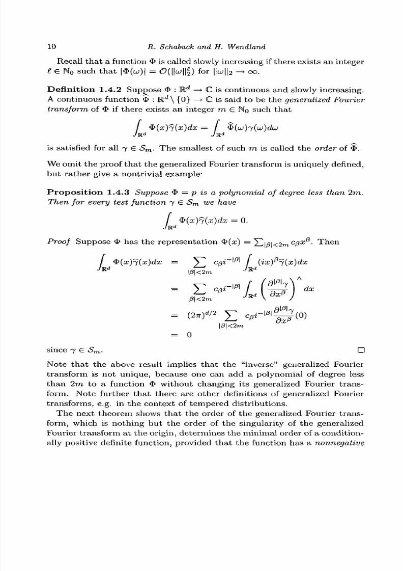
Recall that a function $ is called slowly increasing if there exists an integer
t E No such that |$(w)| = O(||w|||) for ||w||2 -» oo.
Definition 1.4.2 Suppose $ : Rd—> C is continuous and slowly increasing.
A continuous function $ : Rd \ {0} —+ C is said to be the generalized Fourier
transform of $ if there exists an integer m £ No such that
dx = /JR*
is satisfied for all 7 e Sm. The smallest of such m is called the order of $.
We omit the proof th at the generalized Fourier transform is uniquely defined,
but rather give a nontrivial example:
Proposition 1.4.3 Suppose $ = p is a polynomial of degree less than 2m.
Then for every test function 7 6 Sm we have
/ {xY){x)dx = 0.
Proof Suppose $ has the representation $(a;) = Y^im^m0^13- Then
$>(x)j(x)dx = y c/3i~l
= 0
since 7 € <Sm. D
Note that the above result implies that the "inverse" generalized Fourier
transform is not unique, because one can add a polynomial of degree less
than 2m to a function $ without changing its generalized Fourier trans-
form. Note further th a t the re are other definitions of generalized Fourier
transforms, e.g. in the context of tempered distributions.
The next theorem shows that the order of the generalized Fourier trans-
form, which is nothing but the order of the singularity of the generalized
Fourier transform at the origin, determines the minimal order of a condition-
ally positive definite function, provided that the function has a nonnegative

8/3/2019 Multivariate Approximation
http://slidepdf.com/reader/full/multivariate-approximation 21/296
Chapter 1 Construction of radial basis functions 11
and nonzero generalized Fourier transform. We will state and prove only
the sufficient part, but point out that the reverse direction also holds. Weneed the following auxiliary result:
L e m m a 1.4.4 Suppose that distinct x\,... , x^ € Kd
and a € CN
\ {0} are
given such that (1.2) is satisfied for all p € 7rm_i(K d). Then
holds for ||w||2 -> 0.
Proof The expansion of the exponential function leads to
N oo .k N
For fixed w € Mdwe have pfc(a;) := ( ^ a ; ) * 6 7rfc(M
d). Thus (1.2) ensures
that the first m — 1 terms vanish:
JV oo .k N
E^'^E^FEM^)*.
which yields the stated behavior. •
T h e o r e m 1.4.5 Suppose $ : Rd
—» C is continuous, slowly increasing, and
possesses a generalized Fourier transform $ of order m which is nonnega tiveand non-vanishing. Then <f> is a translation-invariant conditionally positive
definite function of order m.
Proof Suppose that distinct xu • • • , xN £ Rd and a e C " \ {0} satisfy (1.2)
for all p e 7rm_i(M d). Define
N
and
j,k=i
where gi{x) = ((/ir)d/2e~
eW
x^. On account of 7f G S and Lemma 1.4.4 we
8/3/2019 Multivariate Approximation
http://slidepdf.com/reader/full/multivariate-approximation 22/296
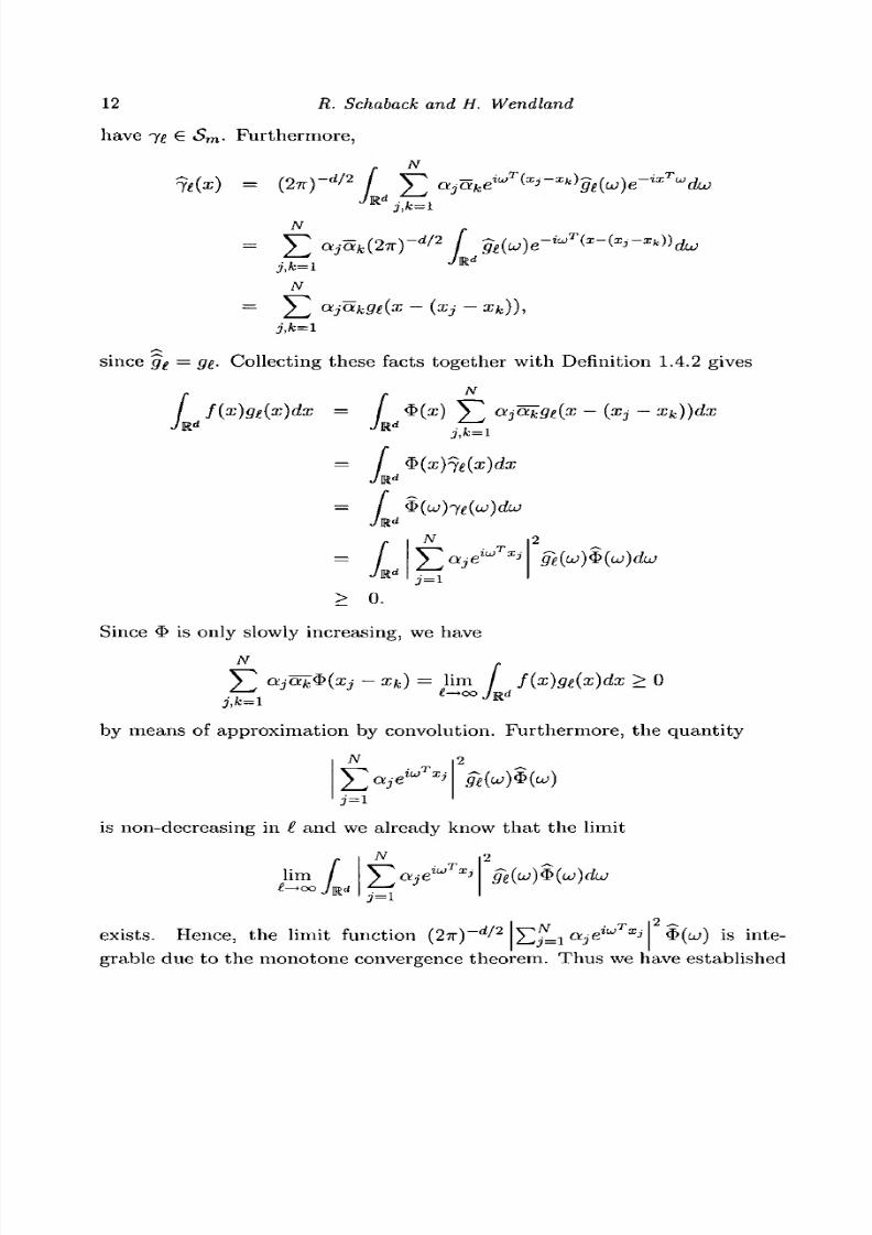
12 R. Schaback and H. Wendland
have 7 € Sm. Furthermore,
N
N
£j,k=i
N
~ (xj - xk)),
since g = ge. Collecting these facts together with Definition 1.4.2 gives
f{x)ge(x)dx = ajoj;ge{x - (XJ - xk))dx
= f $(w;AT
> 0.
Since $ is only slowly increasing, we have
fj - xk) = lim / f(x)ge(x)dx > 0
by means of approximation by convolution. Furthermore, the quantity
JV 2
is non-decreasing in £ and we already know that the limit
_ / V _ 2
lim
is inte-xists. Hence, the limit function (27r)~d/2
J2jLi ot.je%u>T
grable due to the monotone convergence theorem. Thus we have established

8/3/2019 Multivariate Approximation
http://slidepdf.com/reader/full/multivariate-approximation 23/296
Chapter 1 Construction of radial basis functions 13
the equality
ixj - Xk) = {2^rd'2 f
This quadratic form cannot vanish if $ is non-vanishing, since the exponen-
tials are linearly independent. •
1.5 Classical radial basis functions
Now we use this generalization of the Bochner approach to compute the
generalized Fourier transforms of the most popular translation-invariant orradial basis functions. Since it will turn out tha t these generalized Fourier
transforms are nonnegative and non-vanishing, we can read off the order
of conditional positive definiteness of the functions from the order of the
singularity of their generalized Fourier transforms at the origin.
We start with the positive definite inverse multiquadrics treated in The-
orem 1.3.4 and use analytic continuation to deal with the case of the con-
ditionally positive definite (non-inverse) multiquadrics. To do this we need
two results on the modified Bessel functions.
Lemma 1.5.1 The modified Bessel function K v, v 6 C, has the uniform
bound
\K v{r)\ < J— e - ' - e 1 3 ^ , r > 0 (1.10)V r
describing its behavior for large r.
Proof W i t h b = |!R(i/)| we have1 f°°\K u(r)\ < - / e - r c
^ Jo
< I- re-rc
* Jo
= Kb(r).
Furthermore, from el > coshi > 1 + ^-, t > 0, we can conclude
Kb(r) < /Jo
rD
r
8/3/2019 Multivariate Approximation
http://slidepdf.com/reader/full/multivariate-approximation 24/296
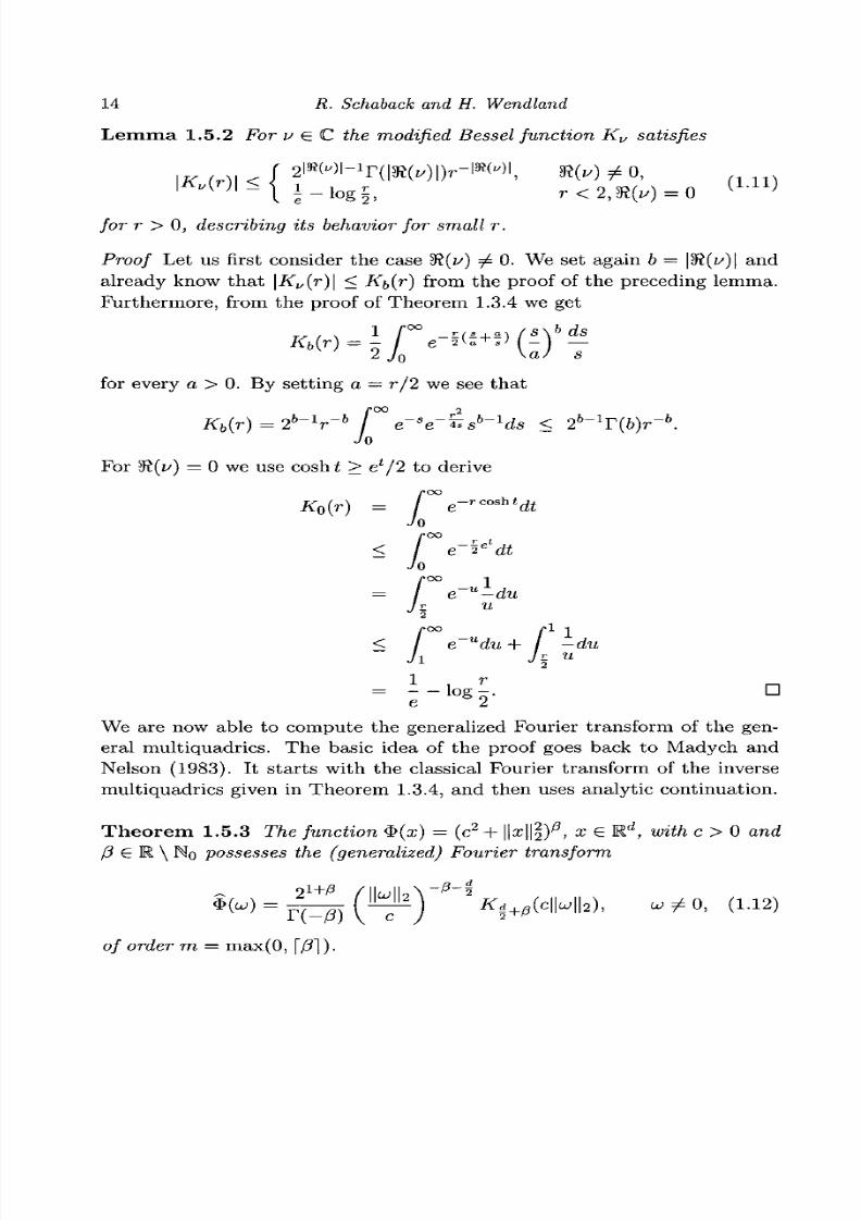
14 R. Schaback and H. Wendland
Lemma 1.5.2 For v eC the modified Bessel function Kv satisfies
Dr-iaMI, H(i/) ± 0,1 " ( ) ! -
for r > 0, describing its behavior for small r.
Proof Let us first consider the case 5R(V) ^ 0. We set again b = \^t(v)\ and
already know that |-Ku(r)| < Kb{r) from the proof of the preceding lemma.
Furthermore, from the proof of Theorem 1.3.4 we get
2 Jo V
for every a > 0. By setting a = r/2 we see that
/•OO 2
Kb{r) = 2b-
1r-
b e-'e-^s^dsJo
For K(^) = 0 we use coshi > el/2 to derive
/•oo
A-0(r) = / e-r cosh tdtJo
< f e-i^dtJo
f°° 1e~u-
h< / 1
-duu
•
We are now able to compute the generalized Fourier transform of the gen-
eral multiquadrics. The basic idea of the proof goes back to Madych and
Nelson (1983). It starts with the classical Fourier transform of the inverse
multiquadrics given in Theorem 1.3.4, and then uses analytic continuation.
Theorem 1.5.3 The function $( i ) = (c2 + \\x\\\)13, x € Rd, with c > 0 and(5 e K \ No possesses the (generalized) Fourier transform
K i+p{c\\Lj\\2), co^O, (1.12)
of order m = max(0,

8/3/2019 Multivariate Approximation
http://slidepdf.com/reader/full/multivariate-approximation 25/296
Chapter 1 Construction of radial basis functions 15
Proof Define G = {A G C : 5R(A) < m} and deno te the r ight-hand s ide of
(1.12) by <pp{w). We are going to show by ana ly t ic cont inua t ion tha t
f ~ fjR d
jRd
is valid for all A G G, where $A(w) = (c2
+ \\UJ\\%)X. Firs t , note that (1 .13)
is valid for A G G with A < —d/2 by Theorem 1.3.4, and, when m > 0, also
for A = 0 , 1 , . . . ,m — 1, by Propos i t ion 1.4.3 and the fact that 1/F(—A) is
zero in these cases. Analytic continuation will lead us to our s ta ted result
if we can show that both s ides of (1-13) exist and are analytic functions in
A. We will do this only for the r ight-hand s ide, s ince the left-hand side can
be handled more eas i ly . Thus we define
/(A) = /JR d
and study this function of A. Suppose C is a closed curve in G. Since <p\ is
an analytic function in A € G it has the representation
for A € I n t C Now suppose that we have already shown that the integrand
in the definition of /(A) can be bounded uniformly on C by an integrable
function. This ensures th at /(A) is well-defined in G and by Fubini's theorem
we can conclude
/(A) = / (p\{uj)i{uj)du
JR
d
= j _ r fvMd {
2iri Jc z -
for A G IntC , which means that / is analytic in G. Thus it remains to bound
the integrand uniformly.Let us first consider the asymptotic behavior in a neighborhood of the
origin, say for ||w||2 < 1/c. If we set b = 5R(A) we can use Lemma 1.5.2 and
7 G Sm to get in the case b ^ —d/2:
8/3/2019 Multivariate Approximation
http://slidepdf.com/reader/full/multivariate-approximation 26/296
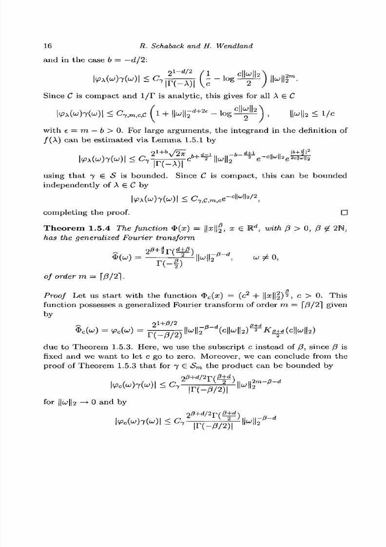
16 R. Schaback and H. Wendland
and in the case b = —d/2:
Since C is compact and 1/F is analytic, this gives for all A € C
IVA(W)7(W)| < C7)TniC)c ( 1 + ||w||2~+ 2 e
- log ——
with e = m — b > 0. For large arguments, the integrand in the definition of
/(A) can be estimated via Lemma 1.5.1 by
using that 7 G <S is bounded. Since C is compact, this can be bounded
independently of A 6 C by
completing the proof. D
Theorem 1.5.4 The function $(x) = ||a;||f, x € Rd, w«ft /3 > 0, /? 0 2N,
/ias i/ie generalized Fourier transform
of order m = [7?/2].
Proof Let us start with the function $c(a;) = (e2
+ H^Hl)2
> c > 0. Thisfunction possesses a generalized Fourier transform of order m = f/3/2] given
by
-r / \ / \ ~ l i l t ^ fl^fl. / ] I II \ £—
due to Theorem 1.5.3. Here, we use the subscript c instead of (5, since (3 is
fixed and we want to let c go to zero. Moreover, we can conclude from the
proof of Theorem 1.5.3 that for 7 G Sm the product can be bounded by
\.~ I. ,\~.t. ,\\ s- n ' 2 / 11, ,ii2m-/3-d
for ||w||2 —> 0 and by
2/3+d/2p/2±d\

8/3/2019 Multivariate Approximation
http://slidepdf.com/reader/full/multivariate-approximation 27/296
Chapter 1 Construction of radial basis functions 17
for ||w||2 —* oo independently of c > 0. Since |$ C (CJ)7(OJ) | can also be
bounded independently of c by an integrable function, we can use the con-vergence theorem of Lebesgue twice to derive
/| |x | |27(a;)da; = l im / ^c(x)^y(x)dx = l im / ipc(uj)j(uj)dx
c— »o J c—>o JR
d
/ '-p/2)
for 7 6 Sm. The last equality follows from
f°° r2
lim r"KJr) = lim 2"" 1\ e~ te~'atv~1dt = 2 J /~T(^ ) ;
see also the proof of Lemma 1.5.2. DT h e o r e m 1 . 5 . 5 The function $ (x ) = | | a ; | | ^ log | |x | |2 , x e Rd, k e N, pos-
sesses i/ie generalized Fourier transform
n.T- n - ! | | w | rd
~2 f c
of order m = k + 1.
Proof For fixed r > 0 and /3 G (2fc, 2fc + 1) we expand the function P i—> r@
using Taylor's theorem to obtainrP
rP = r2k + (P - 2k)r2k logr + / (p - t)rl logr dt. (1.14)
From Theorem 1.5.4 we know the generalized Fourier transform of the func-tion x i—> ||rc||2 of order m = \P/2\ = k + 1. From Proposition 1.4.3 we seethat the generalized Fourier transform of order m of the function x H-> ||x||
2>
fc
equals zero. Thus we can conclude from (1.14) that for any test function
7 e 5 m
/T lnCT T oO/l T W T I I IIT " T I 'Vf'7*l/r/'T
I I 2 ^ o 1 1 2 / \**^) t * « */
— ^ p / I I *" I o — I 1 2 / J \ ) ***
p
— n T n lOP" T o'Vl T W f (IT
Rd
p
P-2R
d 2k
8/3/2019 Multivariate Approximation
http://slidepdf.com/reader/full/multivariate-approximation 28/296
18 R. Schaback and H. Wendland
) r
-§)J- 2k)
for P —> 2k. Furthermore, we know from the property F(.?)r(l — z)
7r/sin(7rz) that
r(-f)(/3-2fc) Tr(P-2k)
Becausesin( f) fcos(f) ^ fc
h m — — — ~ h m =— = —( —1) ,/3—2fc P -2k 0^2k 1 2
we see t h a t
lim _ i = (—l)fc-|-1fc!/2.
0-2fcr(-f)(/?-2AO
Now we can apply the theorem of dominated convergence to get
x\\f log \\x\\ry(x)dx = 22fc+d/2r(fc + d/2)(-i)k+ 1^
for all 7 € 5 m , which gives the stated generalized Fourier transform. •
Now it is easy to decide whether the functions just investigated are con-
ditionally positive definite. As mentioned before, we state the result with
the minimal m.
Corollary 1.5.6 The following functions $ : Rd —» R are conditionally
positive definite of order m:
. $(x) = ( - l ) K V + ||x||2y», p > 0, P £ 2N, m = \P],
. $(i) = (c2 + Hxll
2)", P < 0, m = 0,
. $(x) = (_i)r/J/2l l^ll^ / 3 > 0 J P , m = \p/2],
• $(x) = (-l)k+1
\\x\\lk
log||a:||2, fceN, m = fc + l.
1.6 Construction via dimension walk
So far we have seen that radial functions that work on Rd for all d > 1,
are nicely characterized by the abstract results of Schoenberg and Micchelli,
while translation-invariant functions for fixed dimensions are best handled
via the Fourier transform, yielding explicit results for further use.
8/3/2019 Multivariate Approximation
http://slidepdf.com/reader/full/multivariate-approximation 29/296
Chapter 1 Construction of radial basis functions 19
Here, we want to investigate radial functions for a fixed space dimen-
sion. Thus we have to take the Fourier transform , bu t we shall make use
of radiality throughout, relying on ideas of Wu (1995) and Schaback and
Wu (1996). Our main goal will be the construction of compactly supported
positive definite radial basis functions for fixed space dimensions.
Theorem 1.6.1 Suppose $ € Li(Rd)nC(Rd) is radial, i.e. $(a;) = </>(||a;||2)J
x g Rd. Then its Fourier transform $ is also radial, i.e.
with
Td<j)(r)=r-!
¥ fJo
and <j> satisfies cf>(t)td~ l € Li[0 , oo).
Proof The case d = 1 follows immediately from
/ 2 \ 1 / 2
J-l/2(t)= I — 1 COSt.
When d > 2, splitting the Fourier integral, and using the representation
of the classical Bessel function Jv via an integral over the sphere
yields
(x) = (27r)-d/2
f ${u)e-ixT
jR d
/•oo
= (27T)-d/2 / td
JO
= (27r)-d/2 r 4>{
Jo
The theorem's second assertion follows from the condition $ £ Li(Rd
) n), and the radiality of $ . D
Theorem 1.6.1 gives us the opportunity to interpret the d-variate Fouriertransform of a radial function via Td as an operator that maps univariate
functions to univariate functions.
Now let us have a closer look at this operator with respect to the space

8/3/2019 Multivariate Approximation
http://slidepdf.com/reader/full/multivariate-approximation 30/296
20 R. Schaback and H. Wendland
dimension. If we use £{z vJv(z)} = zvJv-\(z) we get via integration by
parts, for d > 3,
rJo
r°° \- / 4>{s)sds )(rt)
Jt J
= r~d+2
t=oo
= r-d+ 2(-l <j>(s)sds)(rt)^-Jd-2(rt = 0
oo / /•oo
/
(r)
whenever the boundary terms vanish. Thus if we define
I(j>(r) := / <p(t)tdt
Jr
we get the following result.
Theorem 1.6.2 //</. 6 C[0, oo) satisfies 11~* 4>{t)td-
1e Li[0, oo), /o r some
d > 3, i/ien we /lane Td{4>) = Td^ilrf1)- This means that <j> is positive
definite on Rd if and only if I<f> is •positive definite on Rd~2. On the other
hand, if for some d > 1, cj> satisfies t i—> ^ ( i ) ^ " 1 e Li[ 0, oo) and cf>(t) —> 0
as t —» oo, and i/ i/ie even extension of (f> to R is in C 2 ( R ) , i/ien ^ ( ^ =
J-d.+i{D<f>). In this situation, the function 4> is positive definite on W 1 if and
only if Dcf> is positive definite on R
d + 2
.
Since both operators / and D are easily com putable and satisfy / =
D~l and D = J " 1 wherever defined, this gives us a very powerful tool for
constructing positive definite functions. For example, we could sta rt with
a very smooth compactly supported function on R 1 and apply the operator
D n times to get a positive definite and compactly supported function on
R2n+1
. Before we give an exam ple, let us note that it is possible to generalize
the operators Td, I, D to step through the dimensions one by one and not
two by two (Schaback and Wu (1996)).
T h e o r e m 1 . 6 . 3 Define <f>i(r) := (1 — r) e+ and ^>d,k by
4>d,k = I 4>[d/2\+k+l-
Then ^>^k *5 compactly supported, a polynomial within its support, and pos-
8/3/2019 Multivariate Approximation
http://slidepdf.com/reader/full/multivariate-approximation 31/296
Chapter 1 Construction of radial basis functions 21
itive definite on K d . In particular, the function 2 0 ( ^ 1 ( r) = (1 — r)^_(4r + 1)
is positive definite on K 3 .
Proof Since the operator / respects the polynomial structure and compact
sup port, we only have to prove positive definiteness. Since
^d<f>d,k = FdI k<t>ld/2\+k+l = Fd+2k<t>y{d+2k)/2\+l
i t remains to show that Fd<t>[d/2i+i IS nonnegative for every space dimension
d. We will follow ideas of Askey (1973) to do this. Let us start with an odd
dimension d = 2n+ 1. Then the Fourier transform is given by
= f\r -Jo
Denoting the right-hand side of the last equation by g(r), we see tha t g is the
convolution g(r) = JQ gi(r — s)g2{s)ds of the functions gi(s) := (s)++ 1 and
g2(s) := s n + 1 / 2 J n _ i / 2 ( s ) . Thu s its Laplace transform Cg(r) = /0°° g{t)e~ rtdt
is the product of the Laplace transforms of g\ and #2 • These transforms can
be computed for r > 0 as
( n + 1 ) !£ 3 i ( r ) = ^ T ^
and
n! 2"
VTF (1 + r2)™+!'
These combine to give
. . , 2 " + 1 / 2 n ! ( n + i ) ! ;
-yv- ^ rn+ l ( 1 + r . 2 )n+ l -
On the other hand, it is well known that the function 1 — cosr has the
Laplace transform . ^ j , , Thus, if p denotes the n-fold convolution of this
function with itself, we get
By the uniqueness of the Laplace transform this leads to
which is clearly nonnegative and not identically zero. For even space dimen-
sion d = In we need only to note that 0i 2n i , i = <t>\ 2n+i i , , . He nce d>, 2n . , ,L 2 -1 L 2 -I L 2 J" ' "
induces a positive definite function on K2n+1 and therefore also on R 2 n . The
8/3/2019 Multivariate Approximation
http://slidepdf.com/reader/full/multivariate-approximation 32/296
22 R. Schaback and H. Wendland
function <p(r) — (1 — r)A
+(Ar + 1) is nothing but 20^3,1, and hence positive
definite on R 3. •
The parameter k in the last theorem controls the smoothness of the basis
function. It can be shown (Wendland (1995)) that <f>^ possesses 2k contin-
uous derivatives as a radial function on Rd and is of minimal degree among
all piecewise polynomial compactly supported functions that are positive
definite on Rd and whose even extensions to E are in C 2f c(R). A different
technique for generating compactly supported radial basis functions is due
to Buhmann (1998), Buhmann (2000a), Buhmann (2000b).
1.7 Co nstru ction of general func tions
So far we have only dealt with translation-invariant (conditionally) posi-
tive definite functions, and most of our work was even restricted to radial
functions. As a consequence, we had to work with basis functions t hat are
(conditionally) positive definite on all of R d. In this section we want to
take a more general approach which allows us to construct positive definite
functions on local domains fi. Consequently, we have to drop Fourier andLaplace transforms, replacing them by expansions into orthogonal systems.
As a by-product, this technique allows us to construct positive definite func-
tions on manifolds, in particular on the sphere.
T h e o r e m 1 . 7 . 1 Suppose Q C R d is measurable. Let ipi,(f2,--- be an or-
thonormal basis for L^iTl) consisting of continuous and bounded functions.
Suppose that the point evaluation functionals are linearly independent on
sp&n {ifj : j € N } . Suppose pn is a sequence o f positive numbers satisfying
n = l
Then
is positive definite on n .
Proof Pr op ert y (1 .15) ensures tha t $ is well-defined and continuo us. Fur-
thermore, we have, for a £ CN and d is t inc t x\,... , x/v € Q, t h a t
N co N
j,k=l n = l
8/3/2019 Multivariate Approximation
http://slidepdf.com/reader/full/multivariate-approximation 33/296
Chapter 1 Construction of radial basis functions 23
Since the point evaluation functionals are linearly independent on span{y>j :
j £ N } , the last expression can only vanish for a = 0. •
Note that the condition on the point evaluation functionals is somewhat
unnatural for the space L2(£l)- It would be more natural to define $ to
be positive definite iff for every linear independent set A = {Ai , . . . Ajv} Q
L2{£1)* and every a S C^ \ {0} the quadratic form
j,fc=i
is positive. But we do not want to pursue this topic any further. Instead, we
want to use Theorem 1.7.1 to give an example of a positive definite function
on a restricted domain.
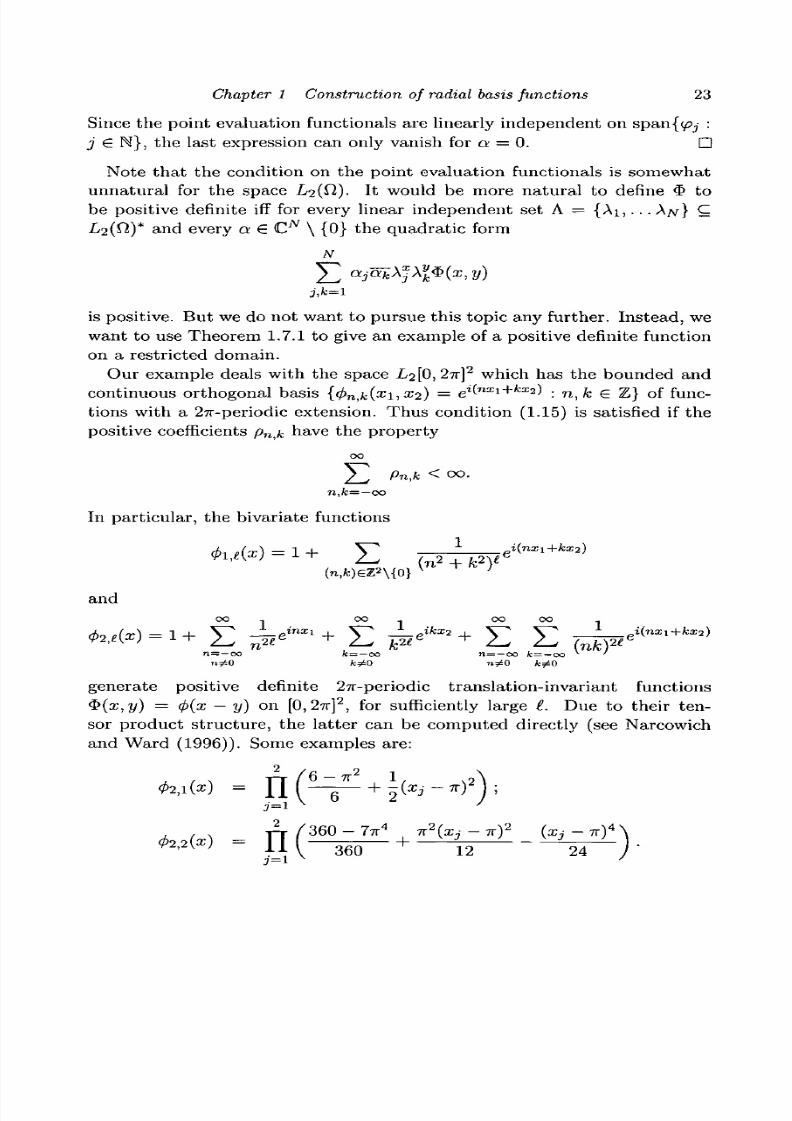
Our example deals with the space L2[0, 2K}2 which has the bounded and
continuous orthogonal basis {4>n,k(^1,^2) = etfnxi+
*:X2
' : n, k € Z} of func-
tions with a 27r-periodic extension. Thus condition (1.15) is satisfied if the
positive coefficients pn<k have the property
00
E pn>k < 00.n,fc=—00
In particular, the bivariate functions
and
i(nx,+kx2)
V^ linx\ , V^ ifex2 i V ^ Y ^
n = — o o fc= —oo n = — o o fc= — o o
generate positive definite 27r-periodic transla tion-invariant functions
$(a;,j/) = <j>(x — y) on [0,27r]2, for sufficiently large L Due to their ten-
sor product structure, the latter can be computed directly (see Narcowich
and Ward (1996)). Some examples are:
3= 1
J ( ^ 3 6 0+
1 2 2 4
8/3/2019 Multivariate Approximation
http://slidepdf.com/reader/full/multivariate-approximation 34/296
24 R. Schaback and H. Wendland
For more examples, see Narcowich and Ward (1996). Of course, this tensor
product approach generalizes to arbitrary space dimension, but the basictechnique is much more general. See Schaback (1999) for the relation to
positive integral operators.
References
Askey, R. (1973). Radial characteristic functions. MRC Technical Report Sum:Report No. 1262, University of Wisconsin.
Bochner, S. (1932). Vorlesungen iiber Fouriersche Integrate. Akademische
Verlagsgesellschaft, Leipzig.Bochner, S. (1933). Monotone funktionen, Stieltjes integrate und harmonischeanalyse. Math. Ann., 108, 378-410.
Buhmann, M.D. (1998). Radial functions on compact support. Proceedings of theEdinburgh Mathematical Society, 4 1 , 33-46.
Buhmann, M.D. (2000a). A new class of radial basis functions with compactsupport. To appear.
Buhmann, M.D. (2000b). This volume.Chang, K.F. (1996a). Strictly positive definite functions. J. Approx. Theory, 87,
148-158.
Chang, K.F. (1996b). Strictly positive definite functions II. Preprint.Guo, K., Hu, S. and Sun, X. (1993). Conditionally positive definite functions andLaplace-Stieltjes integrals. J. Approx. Theory, 74, 249-265.
Madych, W.R. and Nelson, S.A. (1983). Multivariate interpolation: a variationaltheory. Manuscript.
Micchelli, C.A. (1986). Interpolation of scattered data: distance matrices andconditionally positive definite functions. Constr. Approx. 2, 11-22.
Narcowich, F.J. and Ward, J.D. (1996). Wavelets associated with periodic basisfunctions. Appl. Comput. Harmonic Anal., 3, 40-56.
Powell, M.J.D. (1987). Radial basis functions for multivariable interpolation: areview. In Algorithms for Approximation, ed. J.C. Mason and M.G. Cox.,pp. 143-167. Clarendon Press, Oxford.
Schaback, R. (1999). A unified theory of radial basis functions (native Hilbertspaces for radial basis functions II). Preprint, Gottingen.
Schaback, R. and Wu, Z. (1996). Operators on radial functions. J. Comp. Appl.Math., 73, 257-270.
Schoenberg, I.J. (1938). Metric spaces and completely monotone functions. Arm.of Math., 39, 811-841.
Wendland, H. (1995). Piecewise polynomial, positive definite and compactlysupported radial functions of minimal degree. AiCM, 4, 389-396.
Wendland, H. (1999). On the smoothness of positive definite and radial functions.
Journal of Computational and Applied Mathematics, 101, 177-188.Widder, D.V. (1946). The Laplace Transform. Princeton University Press,
Princeton.Wu, Z. (1995). Multivariate compactly supported positive definite radial
functions. AiCM, 4, 283-292.

8/3/2019 Multivariate Approximation
http://slidepdf.com/reader/full/multivariate-approximation 35/296
Approximation and interpolation with radial
functionsM.D. BUHMANN
A b s t r a c t
This chapter gives a short, up-to -date survey of some recent developments in
the research on radial basis functions. Among its other new achievements,
we consider results on convergence rates of interpolation with radial basis
functions, and also recent contributions on approximation on spheres and
on computation of interpolants with Krylov space methods.
2.1 Introduction
Research into radial basis functions is an imm ensely active and fruitful field
at present and it is important and worthwhile to stand back and summarize
the newest developments from time to time. In brief, this is the goal of this
chapter, although we will by necessity be far from comprehensive. One of the
most important aspects from the perspective of approximation theorists is
the accuracy of approximation with radial basis functions when the centers
are scattered . This is a subject quite suitab le to begin this review with, as
the whole development of radial basis functions was initiated by Duchon's
contributions (1976,1978,1979) on exactly this question in a special context,
especially for thin-plate splines approximation in R 2.
Before we begin, we recall what is understood by approximation and in-
terpo lation by radial basis function. We always sta rt w ith a univaria te
continuous function - the radial function - <j) that is radialized by composi-
tion with the Euclidean norm on R n , or a suitable replacement thereof when
we are working on an (n — 1) sphere in n-dimensional Euclidean space. Of
course, due to radialization, we are no longer in a un ivariate setting and this
is not a univariate theory. We are, in addition, given "centers" f from a fi-
nite set E of distinct points in R n (or in a compact subset £1 thereof, or from
the sphere) which are simultaneously used for shifting the radial basis func-
25
8/3/2019 Multivariate Approximation
http://slidepdf.com/reader/full/multivariate-approximation 36/296
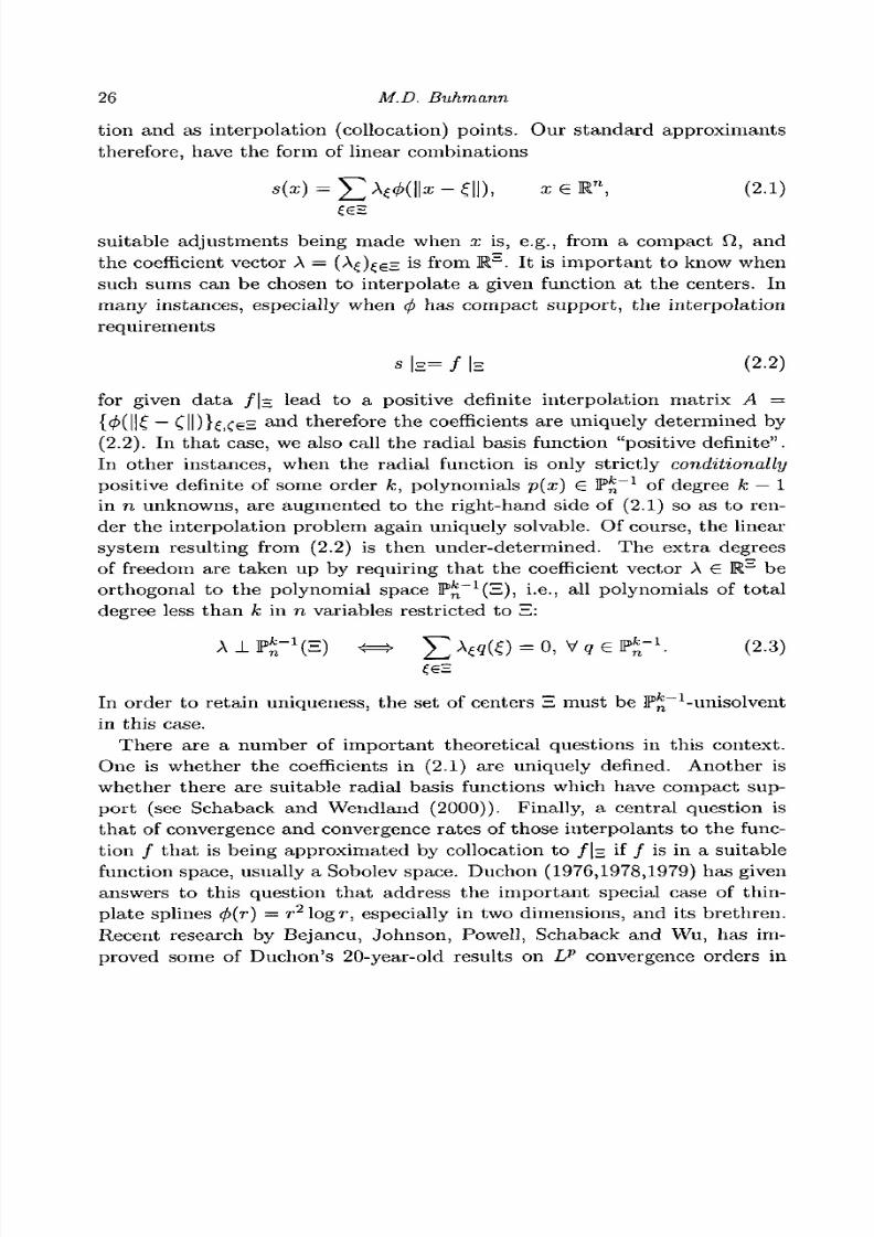
26 M.D. Buhmann
tion and as interpolation (collocation) points. Our standard approximants
therefore, have the form of linear combinations
- £ | | ) , x e l " , (2.1)
suitable adjustments being made when x is, e.g., from a compact 0, and
the coefficient vector A = (A^)^£2 is from R = . It is important to know when
such sums can be chosen to interpolate a given function at the centers. In
many instances, especially when <j> has compact support, the interpolation
requirements
s |== / \s (2.2)
for given data f\-= lead to a positive definite interpolation matrix A =
{<KII£ ~ (IDI^.CeEa n
d therefore the coefficients are uniquely determined by
(2.2). In th at case, we also call the radia l basis function "positive definite".
In other instances, when the radial function is only strictly conditionally
positive definite of some order k, polynomials p(x) G P^"1
of degree k — 1
in n unknowns, are augmented to the right-hand side of (2.1) so as to ren-der the interpolation problem again uniquely solvable. Of course, the linear
system resulting from (2.2) is then under-de termined. The ex tra degrees
of freedom are taken up by requiring that the coefficient vector A € R~ be
orthogonal to the polynomial space F*""1(S), i.e., all polynomials of total
degree less than k in n variables restricted to E:
= 0, V g e P ^1 . (2.3)
In order to retain uniqueness, the set of centers E must be P^~1-unisolvent
in this case.
There are a number of important theoretical questions in this context.
One is whether th e coefficients in (2.1) are uniquely defined. Another is
whether there are suitable radial basis functions which have compact sup-
port (see Schaback and Wendland (2000)). Finally, a central question is
that of convergence and convergence rates of those interpolants to the func-
tion / th at is being approximated by collocation to / |= if / is in a suitable
function space, usually a Sobolev space. Duchon (1976,1978,1979) has given
answers to this question that address the important special case of thin-
plate splines <f)(r) = r2logr, especially in two dimensions, and its brethren.
Recent research by Bejancu, Johnson, Powell, Schaback and Wu, has im-
proved some of Duchon's 20-year-old results on Lp convergence orders in

8/3/2019 Multivariate Approximation
http://slidepdf.com/reader/full/multivariate-approximation 37/296
Chapter 2 Approximation with radial functions 27
various directions, including inverse theorems and theorems about optimal-
ity of convergence orders. Several of these relevant results we address in the
following section, and they hold in all dimensions.
Since this book also contains another chapter (by Schaback and Wend-
land) on radial basis functions, where much attention is given to those func-
tions with compact support, we only devote a short section to compactly
supported 0s. They have many applications, for instance for numerical so-
lutions of partial differential equations, when those radial functions are used
because they can act as finite elements, and they are being tested at the
moment by several researchers for this very purpose. (See, e.g., Fasshauer
(1999), Franke and Schaback (1998), Pollandt (1997).)
In Section 2.4, several recent results about the efficient implementation of
radial basis function interpolation by Krylov space methods are presented,
notably iterative methods with guaranteed convergence, for the computa-
tion of interpolants when the number |E| of centers is very large. This
is then necessary because no direct or simple iterative methods will work
satisfactorily, the matrices resulting from (2.2) and (2.3) being large and ill-
conditioned and sometimes exceptionally so with exponentially increasing
condition numbers (Schaback (1994)).
The final section is devoted to convergence questions for radial basis func-
tions on spheres. The multitude of possible applications (Hardy (1990)) of
radial basis functions for interpolating data, especially on the earth's surface,
be it potential or temperature data for instance, has led many researchers
to consider the question of how to approximate accurately and efficiently
when the data are from a sphere and when the whole idea of distance that
goes into the definition of the above approximants is adjusted properly todistances on spheres, i.e. geodesic distances.
Of course, this brief review is not comprehensive and covers material from
the author's perspective. However, in conjunction with the chapter by Sch-
aback and Wendland, most issues on radial basis functions which are cur-
rently being investigated should be accessible to the reader.
2.2 Convergence rates
The paradigm of globally supported radial basis functions is the thin-plate
spline 4>{r) = r2
log r in two dimensions, and more generally, radial basis
functions of thin-plate spline type in n dimensions, namely,
I r2k
~n
log r if 2k — n is an even integer,4>(r) = < (2.4)
i rzn n if 2fc — n is not an even integer,
8/3/2019 Multivariate Approximation
http://slidepdf.com/reader/full/multivariate-approximation 38/296
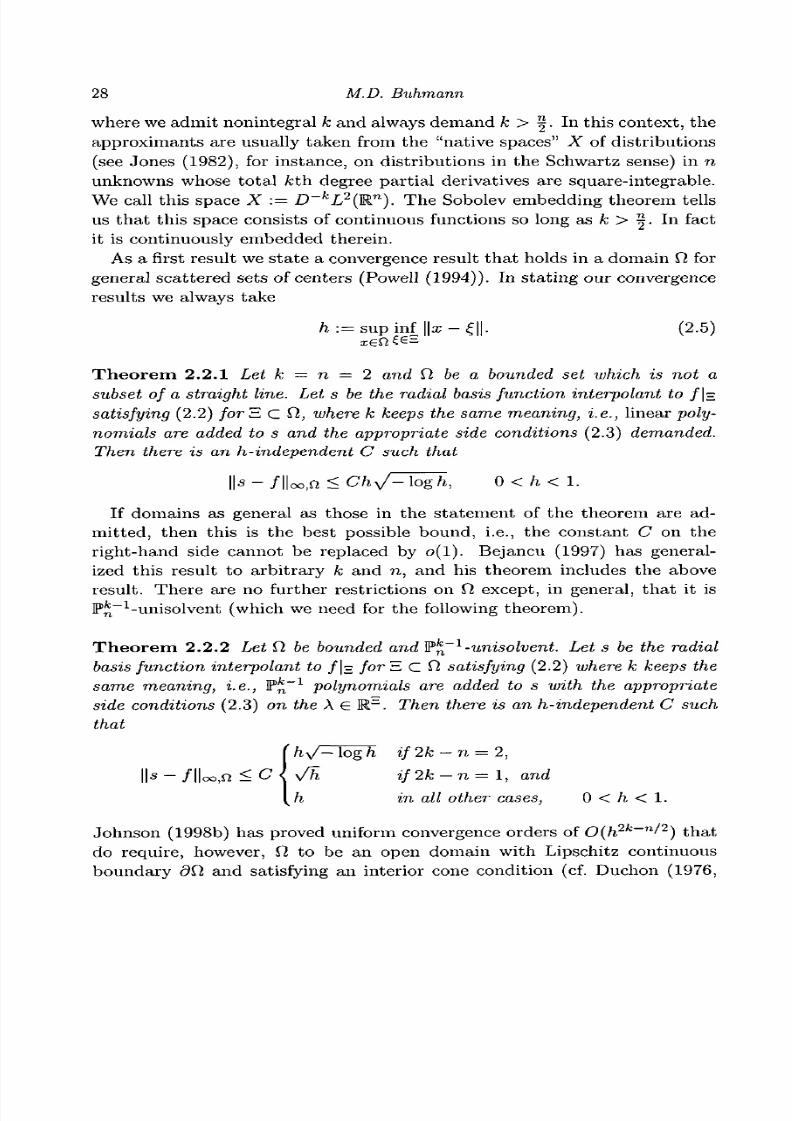
28 M.D. Buhmann
where we admit nonintegral k and always demand k > | . In this context, the
approximants are usually taken from the "native spaces" X of distributions
(see Jones (1982), for instance, on distributions in the Schwartz sense) in n
unknowns whose total fcth degree partial derivatives are square-integrable.
We call this space X := D~kL
2{W
l). The Sobolev embedding theorem tells
us that this space consists of continuous functions so long as k > ^. In fact
it is continuously embedded therein.
As a first result we state a convergence result that holds in a domain fl for
general scattered sets of centers (Powell (1994)). In stating our convergence
results we always take
/i := su pi nf ||a ;-£ ||. (2.5)
Theorem 2.2.1 Let k = n = 2 and Q, be a bounded set which is not a
subset of a straight line. Let s be the radial basis function interpolant to f\=
satisfying (2.2) forE C Cl, where k keeps the same meaning, i.e., linear poly-
nomials are added to s and the appropriate side conditions (2.3) demanded.
Then there is an h-independent C such that
0<h<l.
If domains as general as those in the statement of the theorem are ad-
mitted, then this is the best possible bound, i.e., the constant C on the
right-hand side cannot be replaced by o(l ). Bejancu (1997) has general-
ized this result to arbitrary k and n, and his theorem includes the above
result. There are no further restrictions on ft except, in general, that it is
P^~1
-unisolvent (which we need for the following theorem).
Theorem 2.2.2 Let O be bounded and P*"1
-unisolvent. Let s be the radial
basis function interpolant to / |= forE C fl satisfying (2.2) where k keeps the
same meaning, i.e., P^"1
polynomials are added to s with the appropriate
side conditions (2.3) on the A € R=. Then there is an h-independent C such
that
{/ iV- log h if 2k -n = 2,
y/h i / 2 f c - n = l , and
h in all other cases, 0 < h < 1.
Johnson (1998b) has proved uniform convergence orders of 0{h 2k~n/2) t h a t
do require, however, fl to be an open domain wi th Lipschi tz cont inuous
b o u n d a r y dfl and satisfying an interior cone condit ion (cf. Duchon (1976,
8/3/2019 Multivariate Approximation
http://slidepdf.com/reader/full/multivariate-approximation 39/296
Chapter 2 Approximation with radial functions 29
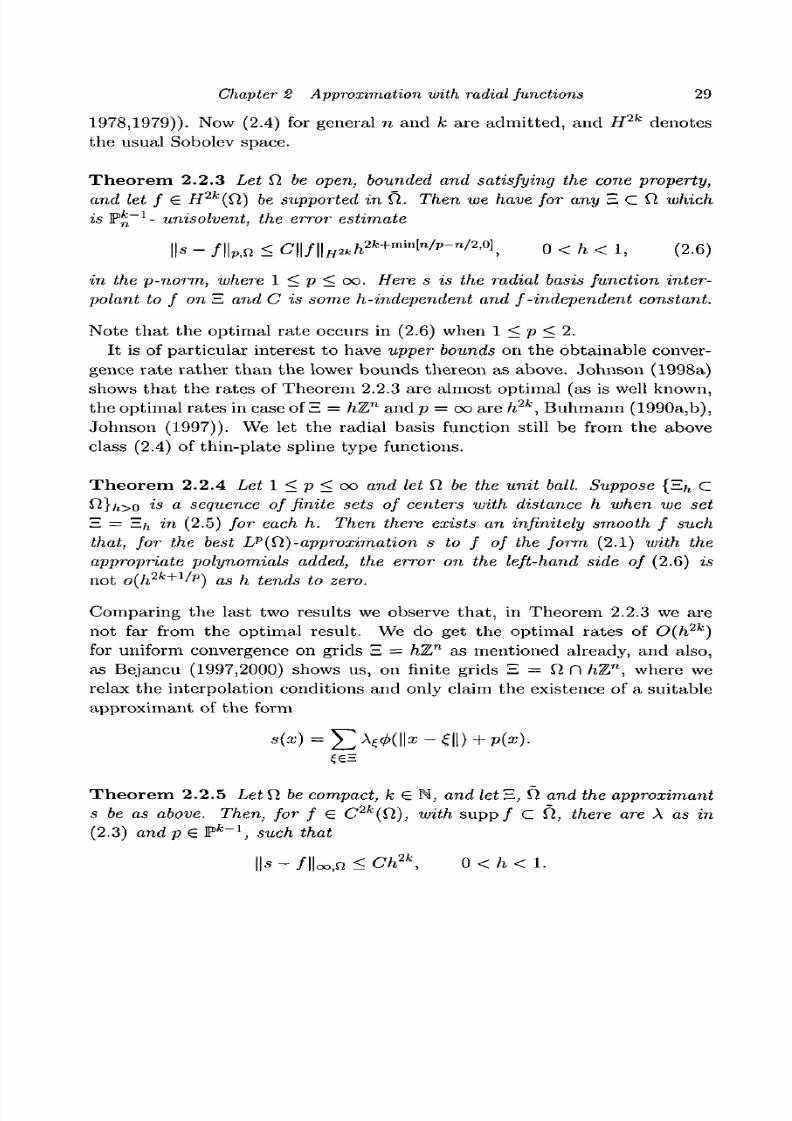
1978,1979)). Now (2.4) for general n and k are admitted, and H2k denotes
the usual Sobolev space.
Theorem 2.2.3 Let fi be open, bounded and satisfying the cone property,
and let f € H2k
(Q) be supported in Cl. Then w e have for any E C ft which
is P ^"1- unisolvent, the error estimate
\\s-f\\P,n<C\\f\\H,kh2k+m'm^- n^, 0 < / K l , (2.6)
in the p-norm, where 1 < p < oo. Here s is the radial basis function inter-
polant to f onE and C is some h-independent and f-independent constant.
Note that the optimal rate occurs in (2.6) when 1 < p < 2.
It is of particular interest to have upper bounds on the obtainable conver-
gence rate rather than the lower bounds thereon as above. Johnson (1998a)
shows that the rates of Theorem 2.2.3 are almost optimal (as is well known,
the optimal ra tes in case of E = hZn
and p = oo are h2k
, Buhmann (1990a,b),
Johnson (1997)). We let the radial basis function still be from the above
class (2.4) of thin-plate spline type functions.
Theorem 2.2.4 Let 1 < p < oo and let 0 be the unit ball. Suppose {E^ C
^}/i>o isa
sequence of finite sets of centers with d istance h when we set
E = S/j in (2.5) for each h. Then there exists an infinitely smooth f such
that, for the best Lf'(0)-approximation s to f of the form (2.1) with the
appropriate polynomials added, the error on the left-hand side of (2.6) is
not o(h2k+1
'p) as h tends to zero.
Comparing the last two results we observe that, in Theorem 2.2.3 we arenot far from th e optimal result. We do get the optimal rates of O(h
2k)
for uniform convergence on grids E = hZn as mentioned already, and also,
as Bejancu (1997,2000) shows us, on finite grids E = fi l~l hZn, where we
relax the interpolation conditions and only claim the existence of a suitable
approximant of the form
Theorem 2.2.5 Let f2 be compact, k G N, and let E, fl and the approx imant
s be as above. Then, for f G C2k
(Q), with s u p p / C Cl, there are A as in
(2.3) andp £ Pf c
~ \ such that
Ch 2k

8/3/2019 Multivariate Approximation
http://slidepdf.com/reader/full/multivariate-approximation 40/296
30 M.D. Buhmann
Looking at Theorem 2.2.4 we see that this is the obtainable (saturation)
order, and an inverse theorem of Schaback and Wendland (1998) tells us
that all functions for which a better order is obtainable must be trivial in
the sense of polyharmonic functions. Tha t is, they are in the kernel of an
iterated Laplace operator. In the following statem ent we use the standard
notation A for the Laplace operator.
Theorem 2.2.6 Let ft be as in Theorem 2.2.3, S C ft a finite set of centers
with distance h as in (2.5) and <f> as in (2.4). If for a given f € C2fc
(fl), and
all compact ft c ft,
then Akf = 0 on ft.
Inverse theorem s may be formulated in a variety of ways. Another way,
from the same paper of Schaback and Wendland, is the following one with
which we close this section. We recall that for a radial basis function with
distributional Fourier transform that agrees with a positive function </>(|| • ||) :Kn \ {0} -> K (Estrada (1998)), the native space norm (which is, strictly
speaking, usually a semi-norm) is
l * <27)
The native space X is the space of all distributio ns / on Kn
for which
(2.7) is finite. In the case of the radial basis functions (2.4), X agrees with
D-k
L2
(Rn
), because ^(HtH)"1
is a constant multiple of ||t||2fc
. Therefore ifwe take for simplicity 0(||£||) = ||<||~
2fc, then equation (2.7) becomes
1f n.i|2fe\f{t)\
2dt.
We have already addressed the notion of conditionally positive functions
in the introduction . The functions (2.4) are strictly conditionally positive
definite of order k subject to a possible sign change. We use the notation
T(X) ~ t(x) if both t(x)/r(x) and r(x)/t(x) are uniformly bounded for theappropriate range of x.
Theorem 2.2.7 Let ft be a domain as in Theorem 2.2.3. Let <fi be strictly
conditionally positive definite of order k and
4>(r) ~ r~2k
, r > 0.
8/3/2019 Multivariate Approximation
http://slidepdf.com/reader/full/multivariate-approximation 41/296
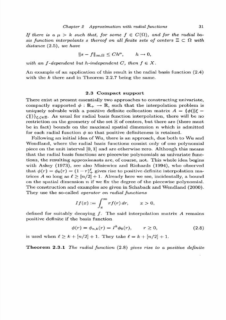
Chapter 2 Approximation with radial junctions 31
/ / there is a \i > k such that, for some f 6 C(Ct), and for the radial ba-
sis function interpolants s thereof on all finite sets of centers E c f l with
distance (2.5), we have
||s -/||oo,n < Ch", h - 0 ,
with an f -dependent but h-independent C, then / e X .
An example of an application of this result is the radial basis function (2.4)
with the k there and in Theorem 2.2.7 being the same.
2.3 Compact support
There exist at present essentially two approaches to constructing univariate,
compactly supported <j> : R+ —> R, such that the interpolation problem is
uniquely solvable with a positive definite collocation matrix A = {<£(||£ —
Cll)}?,CeH- As usual for radial basis function interpolation, there will be no
restriction on the geometry of the set H of centers, but there are (there must
be in fact) bounds on the maximal spatial dimension n which is admitted
for each radial function <f> so that positive definiteness is retained.
Following an initial idea of Wu, there is an approach, due both to Wu and
Wendland, where the radial basis functions consist only of one polynomial
piece on the unit interval [0,1] and are otherwise zero. Although this means
that the radial basis functions are piecewise polynomials as univariate func-
tions, the resulting approximants are, of course, not. This whole idea begins
with Askey (1973), see also Misiewicz and Richards (1994), who observed
that (p(r) = 4>o(r) = (1 — r)+ gives rise to positive definite interpolation ma-
trices A so long as I > [n/2] + 1. Already here we see, incidentally, a bound
on the spatial dimension n if we fix the degree of the piecewise polynomial.
The construction and examples are given in Schaback and Wendland (2000).
They use the so-called operator on radial functions
If(x) := f rf(r)dr, x > 0,Jx
denned for suitably decaying / . The said interpolation m atrix A remains
positive definite if the basis function
<P(r) = 4>n,k(r) = Ik4>o(r), r > 0, (2.8)
is used when (.>k+ [n/2] + 1. They take t = k + [n/2] + 1.
Theorem 2.3.1 The radial function (2.8) gives rise to a positive definite
8/3/2019 Multivariate Approximation
http://slidepdf.com/reader/full/multivariate-approximation 42/296
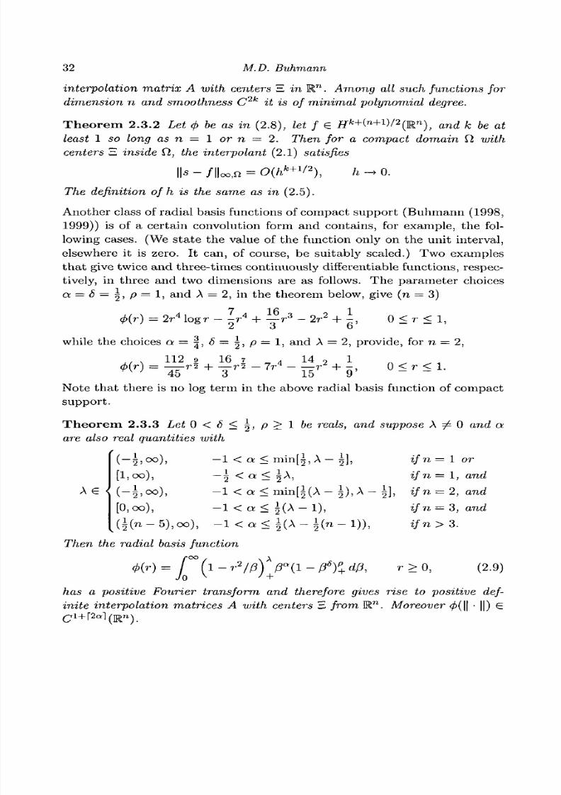
32 M.D. Buhmann
interpolation matrix A with centers E inRn. Among all such functions for
dimension n and smoothness C2k
it is of minimal polynomial degree.
T h e o r e m 2.3.2 Let <f> be as in (2.8), let f € Hk+
(n+ 1
V2(M .
n), and k be at
least 1 so long as n = 1 or n = 2. Then for a compact domain Q, with
centers E inside fl, the interpolant (2.1) satisfies
The definition of h is the same as in (2.5).
Another c lass of radial basis functions of compact suppor t (Buhmann (1998,1999)) is of a certain convolution form and conta ins , for example , the fol-
lowing cases. (We state the value of the function only on the unit interval ,
elsewhere it is zero. It can , of course , be suitably scaled.) Two examples
that give twice and three-t imes continuously differentiable functions, respec-
tively, in th ree and two dimensions are as follows. The parameter choices
a = 6 = T£, p= 1, and A = 2, in th e theorem below, give (n = 3)
7 1 (\ 1
4>{r) = 2 r
4
l o g r - - r
4
+ — r
3
- 2r
2
+ - , 0 < r < 1,
while the choices a = | , ^ = £ , p = l , and A = 2, provide, for n = 2,
jj 16 7 _ 4 _ 14 2 J- Q < < 1
45 3 15 9 ' ~ ~
Note tha t there is no log term in the above radial basis function of compac t
suppor t .
T h e o r e m 2.3 .3 Let 0 < < 5 < | , p > 1 6 e reals, and suppose A ^ 0 and a
are also real quantities with
(—5,00), —1 < a < m inj^ , A — 5]) if n — 1 or
if n = 1, and
2), A— j ] , ifn = 2, and
[0, 00), — 1 < a < j (A — 1), if n = 3 , and
(5(71-5), 00), - 1 < a < i(A - \{n - 1)), ifn>3.
Then the radial basis function
<f>(r)= [ ( l - r2/ p Y P
a(l-P
s)p+dP, r > 0 , (2.9)
Jov
' +has a positive Fourier transform and therefore gives rise to positive def-
inite interpolation matrices A with centers S from W1. Moreover 0( | | • ||) €

8/3/2019 Multivariate Approximation
http://slidepdf.com/reader/full/multivariate-approximation 43/296
Chapter 2 Approximation with radial functions 33
Note that in the statement of the following theorem, the approximand / is
continuous by the Sobolev embedding theorem since 1 + a is positive by the
conditions in the previous theorem.
Theorem 2.3.4 Let <f> be as in the previous theorem and suppose addition-
ally p > 1 and 2a < A — n/2 — 3 + |_pj • Let E be a finite set of dis-
tinct centers in a compact domain Q. Let s be the interpolant (2.1) to
f e L2(R
n) n D~
nl2~
x~
aL
2(W
l): scaled of the form (for a positive scaling
parameter r\)
with the interpolation conditions (s — / ) | E = 0 satisfied. Then the uniform
convergence estimate
11/ - «||oo,n <
holds for h —> 0 and positive bounded rj, the positive constant C being inde-
pendent of both h and r\.
2.4 Iterative methods for implementat ion
The topic we wish to discuss in this section is the practical computation
of radial basis function interpolation in the thin-plate spline case. For this
there is a Krylov space method which uses local Lagrange functions, related
to the so-called domain decomposition methods. Another highly relevant
and useful class of methods are the fast multipole approaches which we do
not describe here (but we recommend reading Beatson and Newsam (1992),
Beatson and Light (1997) and Beatson et al. (1998)). Like the fast multipole
methods, the Krylov space algorithm (Faul and Powell (1999), see also Saad
and Schultz (1986)) is iterative and depends on an initial structuring of the
centers E prior to the start of the iteration. This initial structuring is less
complicated than the fairly sophisticated hierarchical structure demanded
for the multipole schemes, especially when n > 2.
We explain the method for n — 2 and thin-plate splines. Hence, the
interpolant we wish to compute has the same form as in the second section
for k = n = 2 and <j>(r) = r2
log r. But we denote by s* the actual interpolant
we seek, whereas s will now denote only the active approximation to s* at
each stage of the algorithm. The basic idea of the algorithm is to derive,
from minimizing \\s — s*||^, an s from the so-called Krylov space, by a line
search method along mutually orthogonal directions. The directions depend
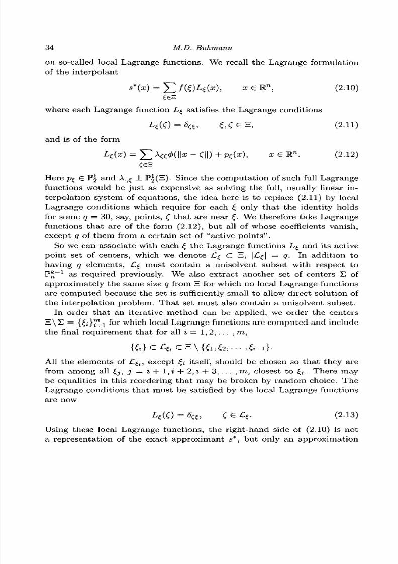
8/3/2019 Multivariate Approximation
http://slidepdf.com/reader/full/multivariate-approximation 44/296
34 M.D. Buhmann
on so-called local Lagrange functions. We recall the Lagrange formulation
of the interpolant
where each Lagrange function L^ satisfies the Lagrange conditions
£?(C) = % £ ,C e H , (2.11)
and is of the form
J2 - Cll) + P«(*), x e R " (2.12)CeH
Here p% € P2 and A.^ ± P^E). Since the computation of such full Lagrange
functions would be just as expensive as solving the full, usually linear in-
terpolation system of equations, the idea here is to replace (2.11) by local
Lagrange conditions which require for each £ only that the identity holds
for some q = 30, say, points, £ that are near £. We therefore take Lagrange
functions that are of the form (2.12), but all of whose coefficients vanish,
except q of them from a certain set of "active points".
So we can associate w ith each £ the Lagrange functions L^ and its active
point set of centers, which we denote C^ C E, |£j | = q. In addition to
having q elements, L^ must contain a unisolvent subset with respect to
P^"1 as required previously. We also extrac t anoth er set of centers E of
approximately the same size q from E for which no local Lagrange functions
are computed because the set is sufficiently small to allow direct solution of
the interpolation problem. That set must also contain a unisolvent subset.In order that an iterative method can be applied, we order the centers
E \ E = {£i}£Li for which local Lagrange functions are computed and include
the final requirement that for alH = 1, 2,... , m,
All the elements of £^, except & itself, should be chosen so that they are
from among all £,, j = i + l,i + 2,i + 3 , . . . ,m , closest to &• There may
be equalities in this reordering that may be broken by random choice. TheLagrange conditions that must be satisfied by the local Lagrange functions
are now
kiO = % C 6 CV (2.13)
Using these local Lagrange functions, the right-hand side of (2.10) is not
a representation of the exact approximant s* , but only an approximation
8/3/2019 Multivariate Approximation
http://slidepdf.com/reader/full/multivariate-approximation 45/296
Chapter 2 Approximation with radial functions 35
thereof. Here is where the iteration comes in. (Of course the Lagrange
functions are computed in advance once and only once, and stored prior to
the beginning of the iterations. This is an O(|E|) process.)
In the iterations, we refine the approximation at each step of the algorithm
by correcting its residual through updates similar to a conjugate gradient
method
s(x)—>s(x)+a-d, (2.14)
where d is a "search direction" defined as
d = r](s* - s) + pd. (2.15)
In (2.14) a is chosen so that \\s — s*\\^ becomes smaller, and in (2.15), d is
the search direction from the previous sweep, P is chosen so that d A. d with
respect to the semi-inner product associated with || • ||^, and ?? is a certain
prescribed operator about which we shall comment below. The correction
(2.15) is added in each sweep of the algorithm.
This completes the sweep of the algorithm. If we started with an approx-
imation s = so = 0 to s*, the sweep replaces Sj by Sj+i that goes into thenext sweep. The stopping criterion can be, for instance, that we terminate
the algorithm if all the residuals on E are sufficiently small. Let U be the
linear space spanned by <f>(\\ • —£||), ( 6 B , plus linear polynomials. Let
Uj be the space spanned by s*,ri(s*),r)(r)(s*)),..., T^'(S*). Those should not
be used as bases for Uj as they are ill-conditioned. Then the goal of the
above choices is to let, in the j th iteration, Sj+\ € Uj be the element which
minimizes \\s — s*||^ among all s € Uj. Now let rj : U i-» U be the map
^ (Lk,s)Lk
k=\At*S*
where (g,g) = ||ff||i, and where a is the full standard thin-plate spline
solution of the interpolation problem
o(g) = s(0, £ € E. (2.16)
Faul and Powell (1999) prove the following for the above method.
Theorem 2.4.1 Let {SJ}'JL0 be a sequence of approximations to s* gener-
ated by so = 0 and the above algorithm, where the radial function is the
thin-plate spline function and n = 2. Then Sj —> s*, as j —> oo.
In fact, their proof shows that for all such operators r\ that recover elements
of the nullspace of || • || ,, and satisfy (r](s),t) = (s,r)(t)) and (s,i](s)) > 0 if
8/3/2019 Multivariate Approximation
http://slidepdf.com/reader/full/multivariate-approximation 46/296
36 M.D. Buhmann
||s||0 > 0, the above method enjoys guaranteed convergence with uniquely
defined search directions. The semi-inner product (•, •) is still the one asso-
ciated with || • ||0. It turns out in practice that this method often provides
excellent accuracy with fewer than ten iterations.
Another approach to the iterative approximation and refinement of the
radial basis function interpolants is that of fast multipole methods. We
briefly outline these here. This is explained in detail in Buhm ann (2000).
However they are sufficiently important that we must, at least, outline the
essentials.
These algorithms are based on analytic expansions of the underlying rad ialfunctions for large argument (see Greengard and Rokhlin (1987)).
The methods require that data be structured in a hierarchical way before
the onset of the iteration, and also an initial computation of the so-called
far-field expansions. The far-field expansions use the fact that radial basis
functions of the form (2.4) are ana lytic except at the origin, even when made
multivariate through composition with Euclidean norms, the derivative dis-
continuity still restricted to the origin, and can be approximated well away
from the origin by a truncated Laurent expansion. The accuracy can bepreset and be arbitrarily small, but of course the cost of the method (here
the multiplier in the operation count), rises with higher accuracy. The mul-
tipliers in the operational count can be large and therefore the method is
only worthwhile if | S | is large, say, 1000 or more. Using the hierarchical
structure of the center set below, this method allows for simultaneous ap-
proximate evaluation of many radial basis function terms, whose centers are
close to each other, by a single finite Laurent expansion. This is cheap, as
long as the argumentx
is far from the "cloud" of centers. By contrast, allradial functions whose translates are close to x are computed exactly and
explicitly, usually with a direct method.
The hierarchical structure of the centers is fundamental to the algorithm
because it decides and orders what is far from and what is near any given
x where we wish to evaluate our function. In a simple two-dimensional
case it is built up as follows. We assume, for ease of exposition, t hat the
£ are fairly uniformly d istribu ted in a square. We form a tree of centers
which contains E as a root, and as the next children, the intersections of thefour quarter squares of the unit square with H. These in turn are divided
into four grandchildren, each in the same fashion, and so on. We stop this
process at a predetermined level that in part determines the accuracy of the
calculation in the end. Each member of this family is called a panel. Recall
that our aim is to evaluate fast at a single point x. Given x, all centers £
that are in the near-field give rise to explicit evaluations of (j>(\\x — £||). The
8/3/2019 Multivariate Approximation
http://slidepdf.com/reader/full/multivariate-approximation 47/296
Chapter 2 Approximation with radial functions 37
so-called near-field consists simply of contributions from all points which are
not "far", according to the following definition: we say x is far away from
a panel T and therefore from all centers in that panel, if there is at least
one more panel between x and T, and if this panel is on the same level of
parenthood as T itself.
Having dealt with the near-field, what remains now is the far-field. We
have to decide how to group the far points. All panels Q are in the evaluation
list of a panel T if Q is either at the same or a coarser (that is, higher) level
than T and every point in T is far away from Q, and if, finally, T contains
a point that is not far away from the parent of Q. Thus the far field of an
x, whose closest center is in a panel T, is the sum of all
such that Q is in the evaluation list of T. For each (2.17), a common Laurent
series is computed. Since we do not know the value of x that is to be inserted
into (2.17), we compute the coefficients of the Laurent series. These do not
depend on x but on H.
Recall that much of the work has to be done at the onset of the algorithm.
In this set-up process, we compute the expansions of the radial function for
large argument, i.e., their coefficients, and store them. When x is provided at
the evaluation stage, we combine those expansions for all centers from each
evaluation list, and finally approximate the whole far field by one Laurent
series. To explain this in detail is long and technical because the various ex-
pansions which are used have to be stated and their accuracy estimated. We
therefore refer, for example, to the paper by Beatson and Newsam (1992).
2.5 Interpolation on spheres
Beginning with Hardy (1990), there was a lot of interest in approximations
on 2 and higher dimensional spheres due to the many applications, for in-
stance in geodesy. In fact the work on radial basis functions on spheres,
in itself, has developed into an important branch of approximation theory.
Freeden and co-workers (1981,1986,1995,1998) have contributed much to
this aspect of the theory. There are excellent and lengthy review papers
available on the work of this group (see the cited references) and others.
One of the main goals of that work is to determine useful classes of radial
basis functions on spheres, e.g, such that interpolants exist and are unique.
We no longer use the conventional Euclidean norm in connection with a
univariate radial function when we approximate on the (n — 1) sphere Sn~
1
8/3/2019 Multivariate Approximation
http://slidepdf.com/reader/full/multivariate-approximation 48/296
38 M.D. Buhmann
within R n . R ath er we apply geodesic dis tances d(x,y) = arccos (xTy) . T h e
standard notions of posit ive definite functions and condit ional posit ive def-
initeness no longer apply, and one has to study new concepts of (str ict ly
condit ionally) posit ive definite functions on the (n — 1) sphere . Th is s tud y
was, as so many other aspects of approximation theory, ini t iated long ago by
Schoenberg (1942). He characterized posit ive definite functions on spheres as
those whose expansions in the series of normalized Gegenbauer polynomials
have non neg ative coefficients. Ex ten din g this work, Xu and C hen ey (1992)
characterized str ict posit ive definiteness on spheres and gave necessary and
sufficient co nd itio ns . It is sufficient t h a t all of th e afo rem en tion ed coeffi-
cients are posit ive. Th is was further generalized by Ro n and Sun (19 96).
They showed that it suffices for strict positive definiteness for a fixed number
m of cen ters, th a t th e coefficients a t > 0 for all k < \m. It is also sufficient
t h a t {k | a t > 0 } con tains arb itra ri ly long sequences of consecu tive od d an d
consecutive even integers k. Quant i ta t ive resul ts on exis tence and s tabi l i ty
of interpolants can be found in Narcowich et al . (1998).
Papers on approximation orders by Jetter et al . (1999) and Levesley et
al. (1999) (see also Dyn et al. (1997)), use native spaces (see below), (semi-)inner products and reproducing kernels (cf . Saitoh (1988) for the theory
of reproducing kernels) to derive approximation orders in a way similar
in fashion to th at su m m arized in Section 2.2. Th ey all use the spherical
harmonics {Vfc }fcLi tn a
t form an orthonormal basis for the d( dimensional
space of polynom ials on the sphere in P ^ ( 5 n - 1 ) PI P ^ ~ 1 ( 5 n ~ 1 ) ± . They are
called spherical harmonics because they are the restr ict ions of polynomials
of total degree £ to the sphere and are in the (^-dimensional kernel of the
Laplace opera tor A.A native space X is defined via the expansion of functions on the sphere
in spher ical harmonics . Namely,
j- o o d( i 2 .2
where
oo de
fco fc=i
and the agk are prescribed posit ive real weights.
The nat ive space has to be equipped both wi th an inner product and a
(semi-)norm. In this case , the inner product can be descr ibed by the double

8/3/2019 Multivariate Approximation
http://slidepdf.com/reader/full/multivariate-approximation 49/296
Chapter 2 Approximation with radial functions 39
sum
oo de
(f,9) = ^2^2—hk9ek,
where the a^ are the coefficients that appear in (2.18). They are still as-
sumed to be positive. The reproducing kernel that results from this Hilbert
space X with the above inner product and that corresponds to the function
of our previous radial basis functions in the native space is, when x and y
are on the sphere, given by
.yeS"-1. (2.20)
1= 0 fc=l
Applying the famous addition theorem (Stein and Weiss (1971)) to <f>(x, y) =
<f>(xTy), this can be written as
oo
(2.21)
ujn-i being the measure of the unit sphere, if the coefficients are constant
with respect to k. Here, Pg is the Gegenbauer polynomial (Abramowitz
and Stegun (1972)) normalized to be one at one. We now use (2.20) or
(2.21) for interpolation on the sphere, in the same place and with the same
centers E as before. Convergence estimates are available from the three
articles mentioned above. Jetter et al. (1999) prove, using the mesh norm
associated with the set of centers E,
h = sup iiifx e S n - l «€ =
the following theorem.
Theorem 2.5.1 Let X and E be as above with the given mesh norm h. Let
K be a positive integer such that h < 1/(2K). Then, for any f € X, there
is a unique interpolant s in
span {«£(£, •) U € E}
that interpolates f on 3 and satisfies the error estimate
8/3/2019 Multivariate Approximation
http://slidepdf.com/reader/full/multivariate-approximation 50/296
40 M.D. Buhmann
Corollary 2.5.2 Let the assumptions of the previous theorem hold and sup-
pose further that |E| + 1 < CxKn~
land
C2 1
1 + K ~ ~ 2K'
Then the said interpolant s provides
h \ (a-n)/2
or
11 / exp( -aC a /2/ . ) \~ \ ft(»-l)/2 ) '
respectively, if d( x maxi</t<^ a^k is bounded by a constant multiple of
(1 + t)~a
for an a > n or by a constant multiple of exp(—a(l + €}) for
a positive a, respectively.
An error estimate due to Levesley et al. (1999) (see also Golitschek and
Light (2000)) which includes strictly conditionally positive definite kernels
for orders K = 1 or K = 2 is for n = 2 (see also Freeden and Hermann (1986),
for a similar, albeit weaker result).
Theorem 2 .5 .3 For X, H, h and K as above, let s be the minimal norm
interpolant to f 6 XK on H (so that to s of Theorem 2.5.1 in particular a
polynomial p £ P J p ^ S2) is added). When <j> is twice continuously differen-
tiate on [1 — e, e] for some e G (0,1), then
\\s~f\\oo <Ch2\\fU.
Acknowledgment
It is a pleasure to thank Oleg Davydov for several thoughtful comments.
ReferencesAskey, R. (1973). Radial characteristic functions. MR.C Report 1262, University of
Wisconsin—Madison.
Abrainowitz, M. and Stegun, I. (1972). Handbook of Mathematical Functions.National Bureau of Stand ards, Washington.
Bea tson, R .K., Cherrie, J.B . and Moat, C .T. (1998). Fast fitting of radial basisfunctions: me thods based on preconditioned GM RES iteration. TechnicalReport Univ., Canterbury, Christchurch.
Bea tson, R.K ., Goodsell, G. and Powell, M .J.D . (1995). On multigrid techniquesfor thin pla te spline interpo lation in two dimensions. Lectures in AppliedMathematics, Vol. 32, pp. 77-97.

8/3/2019 Multivariate Approximation
http://slidepdf.com/reader/full/multivariate-approximation 51/296
Chapter 2 Approxim ation with radial functions 41
Beatson, R.K. and Light, W.A. (1997). Fast evaluation of radial basis functions:methods for 2-dimensional polyharmonic splines. IMA J. Numer. Anal, 17,
343-372.Beatson, R.K. and Newsam, G.N. (1992). Fast evaluation of radial basis functions:
I. Comput. Math. Appi, 24(12) , 7-19.Bejancu, A. (1997). The uniform convergence of multivariate natural splines.
DAMTP Technical Report, Univ. Cambridge.Bejancu, A. (2000). On the accuracy of surface spline approximation and
interpolation to bump functions. DAMTP Technical Report, Univ.Cambridge.
Buhmann, M.D. (1990a). Multivariate interpolation in odd - dimensionalEuclidean spaces using multiquadrics. Constr. Approx., 6, 21-34.
Buhmann, M.D. (1990b). Multivariate cardinal-interpolation with radial-basisfunctions. Constr. Approx., 6, 225-255.
Buhmann, M.D. (1998). Radial functions on compact support. Proceedings of theEdinburgh Mathematical Society, 41 , 33-46.
Buhmann, M.D. (1999). A new class of radial basis functions with compact
support. Technical Report, University of Dortmund.Buhmann, M.D. (2000). Radial basis functions. Ada Numerica, 9, 1-37.Duchon, J. (1976). Interpolation des fonctions de deux variables suivant le
principe de la flexion des plaques minces. Rev. Frangaise Autom at. Informat.
Rech. Oper. Anal. Numer., 10, 5-12.Duchon, J. (1978). Sur l'erreur d !interpolation des fonctions de plusieurs variablespars les £>m-splines. Rev. Francaise Autom at. Informat. Rech. Oper. Anal.Numer. , 12, 325-334.
Duchon, J. (1979). Splines minimizing rotation—invariate semi—norms in Sobolevspaces. In Constructive Theory of Functions of Several Variables, ed .W. Schempp and K. Zeller, pp. 85-100. Springer, Berlin-Heidelberg.
Dyn, N., Narcowich, F.J. and Ward, J.D. (1997). A framework for interpolationand approximation on Riemannian manifolds. In Approximation andOptimization, Tributes to M.J.D. Powell, ed. M.D. Buhmann and A. Iserles,
pp. 133-144. Cambridge University Press, Cambridge.Estrada, R. (1998). Regularization of distributions. Int. J. Math. Math. Sci., 21,625-636.
Fasshauer, G. (1999). Solving differential equations with radial basis functions:multilevel methods and smoothing. Technical Report, IIT Chicago.
Faul, A.C. and Powell, M.J.D. (1998). Proof of convergence of an iterative
technique for thin plate spline interpolation in two dimensions. DAMTPTechnical Report, Univ. Cambridge.
Faul, A.C. and Powell, M.J.D. (1999). Krylov subspace methods for radial basisfunction interpolation. DAMTP Technical Report, Univ. Cambridge.
Floater, M. and Iske, A. (1996). Multistep scattered data interpolation usingcompactly supported radial basis functions. J. Comp. Appl. Math., 73, 65-78.
Franke, C. and Schaback, R. (1998). Solving partial differential equations bycollocation using radial basis functions. Comput. Math. Appl., 93, 72-83.
Freeden, W. (1981). On spherical spline interpolation and approximation. Math.Meth. in Appl. Sci, 3, 551-575.
Freeden, W. and Hermann, P. (1986). Uniform approximation by harmonicsplines. Math. Z., 193, 265-275.

8/3/2019 Multivariate Approximation
http://slidepdf.com/reader/full/multivariate-approximation 52/296
42 M.D. Buhmann
Freeden, W., Gervens, T. and Schreiner, M. (1998). Constructive Approximationon the Sphere. Oxford Science Publications, Clarendon Press.
Freeden, W., Schreiner, M. and Pranke, R. (1995). A survey on spherical splineapproximation. Technical Report 95-157, Univ. Kaiserslautern.
Golitschek, M.V. and Light, W.A. (2000). Interpolation by polynomials and radialbasis functions on spheres. Preprint.
Greengard, L. and Rokhlin, V. (1987). A fast algorithm for particle simulations.
J. Comput. Physics, 73, 325-348.Hardy, R.L. (1990). Theory and applications of the multiquadric-biharmonic
method. Comput. Math. Appl, 19, 163-208.Jetter, K., Stockier J. and Ward, J.D. (1999). Error estimates for scattered data
interpolation on spheres. Math. Comp., 68, 733-747.
Johnson, M.J. (1997). An upper bound on the approximation power of principalshift-invariant spaces. Constr. Approx., 13 , 155-176.
Johnson, M.J. (1998a). A bound on the approximation order of surface splines.Constr. Approx., 14, 429-438.
Johnson, M.J. (1998b). On the error in surface spline interpolation of a compactlysupported function. Manuscript, Univ. Kuwait.
Jones, D.S. (1982). The Theory of G eneralised Functions. Cambridge University
Press, Cambridge.Levesley, J., Light, W.A., Ragozin, D. and Sun, X. (1999). A simple approach to
the variational theory for interpolation on spheres. In Approximation Theory
Bommerholz 1998, ed. M.D. Buhmann, M. Felten, D. Mache and M.W.Miiller. Birkhauser, Basel.
Micchelli, C.A. (1986). Interpolation of scattered data: distance matrices andconditionally positive definite functions. Constr. Approx., 1, 11-22.
Misiewicz, J.K. and Richards, D.St.P. (1994). Positivity of integrals of Besselfunctions. SIAM J. Math. Anal, 25, 596-601.
Narcowich, F., Sivakumar, N. and Ward, J.D. (1998). Stability results forscattered data interpolation on Euclidean spheres. Adv. Comp. Math., 8,137-163.
Pollandt, R. (1997). Solving nonlinear equations of mechanics with the boundary
element method and radial basis functions. Internat. J. for NumericalMethods in Engineering, 40, 61-73.
Pottmann, H. and Eck, M. (1999). Modified multiquadric methods for scattereddata interpolation over the sphere. Comput. Aided Geom. Design, 7, 313-322.
Powell, M.J.D. (1992). The theory of radial basis function approximation in 1990.In Advances in Num erical Analysis II: Wavelets, Subdivision, and RadialFunctions, ed. W.A. Light, pp. 105-210. Oxford University Press, Oxford.
Powell, M.J.D. (1993). Truncated Laurent expansions for the fast evaluation ofthin plate splines. Numer. Algorithms, 5, 99-120.
Powell, M.J.D. (1994). The uniform convergence of thin-plate spline interpolation
in two dimensions. Numer. Math., 67, 107-128.Ron, A. and Sun, X. (1996). Strictly positive definite functions on spheres in
Euclidean spaces. Math. Comp., 65, 1513-1530.Saad, Y. and Schultz, M.H. (1986). GMRES: a generalized minimum residual
algorithm for solving nonsymmetric linear systems. SIAM J. Sci. Stat.Comp., 7, 856-869.
Saitoh, S. (1988). Theory of Reproducing Kernels and its Applications. Longman,Harlow.

8/3/2019 Multivariate Approximation
http://slidepdf.com/reader/full/multivariate-approximation 53/296
Chapter 2 Approximation with radial functions 43
Schaback, R. (1994). Lower bounds for norms of inverses of interpolation matricesfor radial basis functions. J. Approx. Theory, 79, 287-306.
Schaback, R. and Wendland, H. (1998). Inverse and saturation theorems for radialbasis function interpolation. Technical Report, Univ. Gottingen.
Schaback, R. and Wendland, H. (2000). Characterization and construction ofradial basis functions. This volume.
Schaback, R. and Wu, Z. (1996). Operators on radial basis functions. J. Cornp.Appl. Math., 73, 257-270.
Schoenberg, I.J. (1942). Positive definite functions on spheres. Duke Math. J., 9,96-108.
Schreiner, M. (1997). On a new condition for strictly positive definite functions onspheres. Proc. AMS, 125, 531-539.
Sibson, R. and Stone, G. (1991). Computation of thin plate splines. SIAM J.Scient. Stat. Corn-put., 12, 1304-1313.
Stein, E.M. and Weiss, G. (1971). Introduction to Fourier Analysis on EuclideanSpaces. Princeton University Press, Princeton.
Steward, J. (1976). Positive definite functions and generalizations, a historicalsurvey. Rocky Mountains Math. J., 6, 409-434.
Wendland, H. (1995). Piecewise polynomial, positive definite and compactlysupported radial functions of minimal degree. Advances in ComputationalMathematics, 4, 389-396.
Wendland, H. (1997). Sobolev-type error estimates for interpolation by radial
basis functions. In Surface Fitting and Multiresolution Methods, ed. A.LeMehaute and L.L. Schumaker, pp. 337-344. Vanderbilt University Press,Nashville.
Wendland, H. (1998). Error estimates for interpolation by radial basis functions ofminimal degree. J. Approx. Theory, 93, 258-272.
Wu, Z. (1992). Hermite-Birkhoff interpolation of scattered data by radial basisfunctions. Approx. Theory Appl., 8, 1-10.
Wu, Z. (1995). Multivariate compactly supported positive definite radialfunctions. Advances in Computational Mathematics, 4, 283-292.
Wu, Z. and Schaback, R. (1993). Local error estimates for radial basis function
interpolation of scattered data. IMA J. Numer. Anal., 13, 13-27.Xu, Y. and Cheney, E.W. (1992). Strictly positive definite functions on spheres.Proc. Amer. Math. Soc, 116, 977-981.
8/3/2019 Multivariate Approximation
http://slidepdf.com/reader/full/multivariate-approximation 54/296
Representing and analyzing scattered data on
spheresH.N. MHASKAR, F.J. NARCOWICH and J.D. WARD
Abstract
Geophysical or meteorological data collected over the surface of the earth
via satellites or ground stations will invariably come from scattered sites.
There are two extremes in the problems one faces in handling such data.
The first is representing sparse da ta by fitting a surface to it. Th is arises
in geodesy in conjunction with measurements of the gravitation field from
satellites, or meteorological measurements - temperature, for example -made at ground stations . The second is analyzing dense data to extract
features of interest. For exam ple, one may wish to process satellite images
for m apping purposes. Between these two extremes there are many other
problems. We will review various aspects of fitting surfaces to scattered da ta,
addressing problems involving interpolation and order of approximation, and
qua dratu res. Analyzing da ta is a more recent problem th at is currently being
addressed via various spherical wavelet schemes, which we will review, along
with multilevel schemes. We close by discussing quadrature methods, whicharise in many of the wavelet schemes as well as some interpolation methods.
3.1 Introduction
3.1.1 Overview
In this survey, we discuss recent progress in the rep resen tation and analysis of
scattered data on spheres. As is the case with R s, many practical problemshave stimulated interest in this direction. More and more da ta is taken
from satellites each year. Th is, in turn , requires for example, improved
image processing techniques for fault detection and for generation of maps.
Meteorological readings (temperature, pressure, etc.) as well as geophysical
44
8/3/2019 Multivariate Approximation
http://slidepdf.com/reader/full/multivariate-approximation 55/296
Chapter 3 Scattered data on spheres 45
data (gravitational field) are a few examples where enhanced representation
and analysis of data capabilities prove useful.
Our domain of consideration is the g-sphere Sq rather than R
s. While
the q-sphere, Sq, shares many similarities with HL
S, there are also significant
differences. Since Sq
is compact, there is no need for "infinite" amounts of
data for the analysis, while if one restricts oneself to compact subdomains
of R5, then the boundary of such sets introduces many difficulties. On the
other hand, all large data sets on the sphere are necessarily scattered. In
other words, there is no analogue to "gridded" data (for data sets larger
than 20). This fact makes the standard Es construction of wavelets on the
sphere inapplicable.
A brief outline of this article is as follows. In Section 3.2 we discuss the
representation of data on Sq. Here we are primarily concerned with in-
terpolation and quasi-interpo lation/approxim ation. Recent progress along
these lines involves families based on spherical basis functions, which are
discussed below. Section 3.3 deals with the analysis of data on Sq. Vari-
ous constructs of wavelets, including continuous wavelet transforms as well
as discrete wavelets, are mentioned here. In addition, we discuss localiza-
tion and uncertainty principles on Sq. Also included in this section is a
brief introduction to multilevel interpolation. Finally, in Section 3.4, vari-
ous numerical schemes for implementing the ideas in the previous sections
are detailed. In both the representation and analysis of scattered data on
spheres, efficient computations of Fourier coefficients and convolutions are
needed. A quick tour of quadrature rules to estimate integrals over the
g-sphere as well as related topics, such as sampling theorems and discrete
Fourier transforms, are also given.
Many au thors have contributed valuable insights into the topics discussed
here. In this regard, we wish to apologize in advance for any omissions, and
also for any other mistakes that we may have made in the preparation of
this article.
3.1.2 Background - spherical harmonics
There are a number of books that treat spherical harmonics and their ap-proximation properties. For classical results on spherical harmonics, there is
the book of Hobson (1965). Later, very useful references are Muller's book
(Miiller (1966)) and, of course, the book by Stein and Weiss (1971). To a
large extent, we will follow Muller's no tation . Let q > 1 be an integer which
will be fixed hroughout the rest of this article, and let S9
be the unit sphere
in the Euclidean space Rq+1
, with d[i,q being its usual area element, which
8/3/2019 Multivariate Approximation
http://slidepdf.com/reader/full/multivariate-approximation 56/296
46 H.N. Mhaskar, F.J. Narcowich and J.D. Ward
is invariant under arbitrary coordinate changes. The volume of Sq is
Corresponding to dfiq, we have the inner product,
(f,g)s"-= f{x)g(x)dfj.q{x),JS "
and Lp(S
q) norms,
I/P
Th e class of all measurable functions / : Sq —* C for which ||/||s«,p < oo
will be denoted by L^S 9 ), with the usual understanding that functions that
are equal almost everywhere are considered equal as elements of V(Sq). All
continuous complex valued functions on Sg will be denoted by C(Sq).
For an integer £ > 0, the restriction to Sq of a homogeneous harmonic
polynomial of degree £ is called a spherical harmonic of degree £. The class of
all spherical harmonics of degree £ will be denoted by Hj, and the class of allspherical harmonics of degree £ < n will be denoted by n ' . Of course, IT' =
0 £ _ o H%, and it comprises the restriction to Sq of all algebraic polynomials
in q + 1 variables of total degree not exceeding n. The dimension of Hq is
given by Miiller (1966), p. 11
and that of II« is E"=o d « -
The spherical harmonics have an intrinsic characterization as the eigen-
functions of Asi> the Laplace—Beltrami operator on Sq. As? is an
elliptic, (unbounded) selfadjoint operator on L2(S
q), invariant under arbi-
trary coordinate changes; its spectrum comprises discrete eigenvalues A^ :=
—£(£ + q — 1), £ = 0 , 1 , . . . , each having finite multiplicity dq. The space H q
can be characterized intrinsically as the eigenspace of As? corresponding to
\( . Hence, for distinct <"s, the Hj's are mutually orthogonal relative to theinner product (•,-)s«; in addition, the closure of their direct sum is all of
L2(S
q). That is, c losure{ © £ # ' } = L
2(S
q). If we choose an orthonormal
basis {Yg tk '• fc = 1,..., rf'} for each Hq, then we automatically have that
the set {Y^fc : £ = 0 , 1 , . . . ; k = l , . . . , d | } is an orthonormal basis for
L2(S
q). (See Narcowich (1995), §IV for a more complete discussion and
further references.)

8/3/2019 Multivariate Approximation
http://slidepdf.com/reader/full/multivariate-approximation 57/296
Chapter 3 Scattered data on spheres 47
The spherical harmonics satisfy the well-known addition formula (Miiller
(1966),Stein and Weiss (1971))
= — Veiq + lix-y), £ = 0 , 1 , . . . ,
where Ve(q + 1; t) is the degree t Legendre polynomial in t, associated with
Sq. The Legendre polynomials are normalized so that Ve(q + 1; 1) = 1, and
satisfy the orthogonality relations
2 \s
- , U!q
1;x)T ' ic (q + l;x)(l — x )2 a x = ~7q~vi,ki
and, up to normalization, are the same as the ultraspherical polynomials
p««-i)/2) ( M u l l e r (1966), p. 33) and the Jacobi polynomials pfo/2-W2-i)
(Szego (1975)).
The addition formula allows us to express a variety of projection operators
directly in terms of simple kernels. For example, the projection of / 6 L2(S
q)
onto Hq
is just
P « / ( x ) : = P r o j f f ? / ( x ) = ^ f Pt(q + l;x- y)f{y)d^(y),e
uq JSq
j q
with the kernel being •^•Vt{q + l ;x • y). For the sequence {Pe}^^ of these
mutually orthogonal projections, we define the order k Cesaro means via
the standard formula,
Replacing the projections above by their kernels yields kernels for En , which
we denote by o 4 ' (x • y). For
| ^ = M l , (3.1)
k fixed, these kernels have L1
norms uniformly bounded in n (Szego (1975)),
say by C.
The Cesaro operators are needed to construct the delayed mean operators
introduced by Stein (1957). These operators have the form
fc+i
£ « * • "£ $ _ ! , n > l , (3.2)
8/3/2019 Multivariate Approximation
http://slidepdf.com/reader/full/multivariate-approximation 58/296
48 H.N. Mhaskar, F.J. Narcowich and J.D. Ward
and reduce to the identity on n ' , provided n is larger than some integer Nq,
that is,
Tik)\ni= ldnl,n>N q. (3.3)
Moreover, the coefficients are bounded independently of n. A simple exam-
ple is the de la Vallee Poussin operator,
T« := 2 ^ - E ^ = ±Pt+ ]£ *LLLPl, n > 1. (3.4)e=o «=n+i
The first sum on the right in (3.4) is the orthogonal projection onto II ' and
the second maps II' to 0. If q is 1 or 2, then because the Cesaro operators
are bounded, the sequence of operators T« ' : L°°(Sq) —> C(S
q) satisfies
ll^n^H < 3C for all n > 1. We remark tha t if q > 3 and k satisfies the
inequality (3.1), then Tn ' has similar properties (cf. Mhaskar et al. (2000),
Theorem 2.1 and Stein (1957), Theorem 1).
3.2 Representing data
In this section, we wish to discuss some past and present developments
concerning scattered-data surface fitting and approximation on the sphere.
Many articles have been written on the subject, including several good,
recent survey articles (Cheney (1995), Fasshauer and Schumaker (1998),
Freeden et al. (1997), Narcowich (1998)). We will focus on approximation/
surface-fitting by positive definite (and related) functions.
Approximation on the sphere has evolved in the same way as approxima-tion on W. The early results focused on approximation with polynomials
(or spherical harmonics) but approximation with other families of functions
were later studied in order to address the shortcomings of polynomial ap-
proximation, such as instability or inability of polynomials to interpolate at
scattered sites, Gibbs' phenomena, the computational expense of evaluating
polynomials of high degree, and global support.
There have been at least three approaches for circumventing some of the
problems mentioned above. One of them concerns the spherical splines orig-inally investigated about 20 years ago by Freeden (1981), Wahba (1981)
and others. These functions have the form <j)(x • y) where x and y are unit
vectors and 4> is a spline-like function defined on [—1,1]. Much has been
written along these lines and for the interested reader we refer to the recent
survey paper (Freeden et al. (1997)). In another direction, locally supported
piecewise polynomials built on triangulated spherical patches and described
8/3/2019 Multivariate Approximation
http://slidepdf.com/reader/full/multivariate-approximation 59/296
Chapter 3 Scattered data on spheres 49
in terms of spherical Bezier nets have recently been investigated by Alfeld et
al. (1996). An excellent review in this direction has been given in Fasshauer
and Schumaker (1998). The third approach originated in a celebrated paper
of Schoenberg (1942), in which the key ideas for interpolation and approxi-
mation on the sphere were introduced.
3.2.1 Interpolation on the sphere
Schoenberg (1942) introduced functions that he termed positive definite on
S'. Let 9(x,y) be the geodesic distance between two points x and y on S' .
A continuous function G(#(x, y)) is said to be a positive definite function
on Sq
if, for every set of points C = {xi,... , x/v}, the N x N matrix with
entries [G(9(xj,Xk))] is self adjoint and positive semi-definite. Schoenberg
(1942) completely classified all such functions in terms of expansions in
ultraspherical (Gegenbauer) polynomials.
Theorem 3.2.1 (Schoenberg (1942)) A continuous function G(8(x,y)) is
a positive definite function on Sq
if and only if
G(0(x, y)) = G(arccos(x • y)) = J^ «^(<? + 1; x • y),
where Ve(q + 1; x • y) is the degree £ Legendre polynomial associated with Sq,
and the ai > 0 decay sufficiently fast for G(9(x, y)) to be continuous in x • y .
Since the invertibility of the matrix Aj^ := [G(9(xj,Xk))] is necessary to
interpolate data f{xj),j = 1,... ,N, from the space span{G(#(x,Xj))}, the
representation theorem of Schoenberg suggests that positive definite fun-
ctions on spheres would be an ideal class of functions for interpolation,
provided the interpolation matrices were invertible for distinct points.
Xu and Cheney (1992) gave a number of interesting conditions on G guar-
anteeing that the matrix [G(#(xj,x/t))] will be positive definite, and there-
fore invertible, for classes of finite subsets C C Sq in which the points are
distinct. We say that G is strictly positive definite of order N if the ma-
trix [G(9(xj,Xk))] is positive definite whenever the set C has cardinality less
than or equal to N. When this happens for all N, we will say that G is
strictly positive definite. One particular condition in Xu and Cheney (1992)
sufficient for G to be strictly positive definite, is that the coefficients in the
expansion of G satisfy ae > 0 for every £. Ron and Sun (1996) shed further
light on the invertibility of the interpolation matrices.
8/3/2019 Multivariate Approximation
http://slidepdf.com/reader/full/multivariate-approximation 60/296
50 H.N. Mhaskar, F.J. Narcowich and J.D. W ard
Theorem 3.2.2 (Ron and Sun (1996)) A function G is strictly positive
definite of order N if the coefficien ts cii,..., a^ / 2 j
are
positive. Moreover,G is strictly positive definite for all orders if the set K := {k € Z+ : a& > 0}
contains arbitrarily long sequences of consecutive even integers, as well as
arbitrarily long sequences of consecutive odd integers.
It is still an open question as to what conditions are both necessary and
sufficient for G to be strictly positive definite, either for finite order or all
orders.
Narcowich (1995) investigated solving very general Hermite interpolation
problems on compact Riemannian manifolds, with data "sampled" by ap-plying arbitrary distributions to smooth functions. One consequence was
that if G is C°° and satisfies the condition that ag > 0 for all £, then it is
strictly positive definite in an even stronger sense than what is discussed
above. The set of point evaluations corresponding to C can be replaced by
a finite set of arbitrary, linearly independent distributions, and the (gener-
alized) interpolation matrices that result will be strictly positive definite.
Analogues hold when G is not C°°, bu t is in a Sobolev space. (See the
discussion below.)
The functions G for which ag > 0 for all t are quite useful; we call them
spherical basis functions (SBFs).
The work described above was directed toward the solvability of various
interpolation problems; it set the stage for the next round of investigations,
which were aimed at answering the question of how well the interpolants
approximate functions from a given smoothness class. Such questions were
investigated in the W case (for scattered data) in a series of papers starting
with Madych and Nelson (1983). A convenient setting for analyzing such
questions is a reproducing kernel Hilbert space whose relevance to interpo-
lation problems was first pointed out in Golomb and Weinberger (1959).
An early work concerning error estimates on the sphere was that of Free-
den. For a given scattered, finite set of points C on the sphere, one defines
the mesh norm 8c of C by
8r '•= maxdist(x, C) = m axm indis t(x, y) , (3.5)
where the distance is the geodesic distance on the sphere. Freeden showed
that interpolants formed from spherical splines converge at rates \8c\T, where
T £ [0,1]. Th e value of T depends on a num ber of factors; see Freeden (1986).
In subsequent years, further application of the Golomb-Weinberger frame-
work (Golomb and Weinberger (1959)) in the case of the sphere produced
results for which the rates of approximation reflected the sm oothness of bo th

8/3/2019 Multivariate Approximation
http://slidepdf.com/reader/full/multivariate-approximation 61/296
Chapter 3 Scattered data on spheres 51
the approximating kernel as well as the function to be approximated. We
give a brief description of these results next. A more complete explanation
of relevant material can be found in Dyn et al. (1997,1999).
We will work in the same setting as Narcowich (1995); namely, we take the
underlying space to be a compact, C°° Riemannian manifold M. Spheres
and tori are of course examples.
We will need to introduce some notation. We will denote the Riemann-
ian metric on A4 by g^j and its inverse by gld
. The corresponding volume
element, inner product, Laplace-Beltrami operator and its eigenvalues and
eigenfunctions, are
dfj,(x) := g(x) J/2dx, where g(x) := detgy(x) > 0
{},9)M •= JM /(x)s(x) d/i(x)
(3-6)
._ jjt/i eigenvalue of A
:= eigenfunction corresponding to
Finally, we let T>' denote the set of all distributions on M, and define the
Sobolev space
H s(M ) = {ueV : ] T .
The (Sobolev) norm for this space is given by
oo N l / 2
One can integrate the product of a kernel K(X, y) in H2S(M x A4) with a
distribution u(y) £ H_S(M), with the resulting distribution being a func-tion in HS{M). In particular, we define
K*U(X)= K(x,y)u(y)d/i(y).JM
Note that "*" is not commutative. In the special case in which u is a
linear combination of point evaluations, u = ^2j=idjSXj, then K*U(X) =
E j L i « j « ( x . x j ) -
A function K 6 H2S(M x Al) is a strictly positive definite kernel if for
every nonzero distribution u G H-S(M ) we have that (U,K*U)M > 0.
Consequently, we can use a strictly positive definite kernel « to define a
norm on H-S(M); namely,
:= \/(U,K*U)M-

8/3/2019 Multivariate Approximation
http://slidepdf.com/reader/full/multivariate-approximation 62/296
52 H.N. Mhaskar, F.J. Narcowich and J.D. Ward
All kernels of the form
^ ) , ak > 0. (3.8)
k= \
are s tr ic t ly posit ive defini te , provided that the aks decay sufficiently fast for
them to be in one of the Sobolev spaces defined above.
In practical applicat ions one often wants interpolants that reproduce ex-
actly some fixed, finite dimensional space of functions - for example, polyno-
mials on R s or spherical harmonics on Sq. In Dyn et al. (1999), conditionally
positive definite kernels were introduced to deal with such problems for gen-eral man ifolds. Le t I be a finite set of indices in Z + , and consid er th e finite
dimensional space defined by S% := s p a n j i ^ : i € 1}. In addition, define the
space of d is t r ibu t ions 5 ^ := {u <E H-S(M ) : (u,F)M = 0 , F € Si} . W e
will say that a selfadjoint, continuous kernel K, in H2S{M x M) is condition-
ally positive definite (CPD) with respect to a finite set of indices T C Z + if
for every u € Sj we have {u , K * U)M > 0. M oreover, if for a ll such t i ^ O
we have (u,K*U)M > 0, then we will say that n is c o n d i t i o n a l l y s t r i c t l y
p o s i t i v e d e f i n i t e (CSPD) on M with respect to Sj. All kernels of the form(3.8) are CSPD for Si, provided only that ak > 0 for all k £ Z + \ J .
The next result gives error es t imates for interpolat ion us ing dis tr ibutions
an d a str ict ly po sitiv e definite ker nel At e H2S(M x M). Let {U J : j =
1 , . . . ,N} be a l inearly independent se t of dis tr ibutions in H-S(M), an d
define the space U := spanJMj : j = 1 , . . . ,N}. The problem is that i f
/ € HS(M ) and if we are given data dk = (M fc , / )^ , the n we want to
find u S U such th at / := K * u satisfies dk = {uu, DM f ° r ^ = 1, • • • ,N .
Equivalently, we want to find c\,... ,CN such th a t / = 5Zj=ic
j
K
*
u
j satisfiesdk = Ylj=i c
j(uk,
K * UJ)M f ° r k = 1 , . . . , N. Because K is strictly positive
definite , the interpolat ion matrix Aj^ := (UJ, n-ku^jM ls positive definite and
invertible, so we can always solve for the CjS and find a unique dis tr ibution
u 6 U such th at / := K*U solves the interpolat ion problem.
How close are / and / ? Let / = n + v, with v e H-S(M). The following
result is a version of the hypercircle inequality (Golomb and Weinberger
(1959)).
T h e o r e m 3 . 2 . 3 (Dyn et al. (1999), Proposition 3.2) Let f = n*v and let
f = K*U be the interpolant described above. If w is an arbitrary distribution
in H-s. then
\{w,f-f)M\
where the distances are computed relative to the norm (3 .7).

8/3/2019 Multivariate Approximation
http://slidepdf.com/reader/full/multivariate-approximation 63/296
Chapter 3 Scattered data on spheres 53
Of course, \(w,f — J)M\ defined above represents the interpolation error
relative to the distribution w 6 H-s. In order for this formulation to be
useful, one must estimate the distances given on the right hand side of the
inequality. Using the notation defined in (3.6), we can state the next result,
which gives a framework for making such estimates.
Theorem 3.2.4 (Dyn et al. (1999), Proposition 3.6) Let n be a positive
integer, s > 0, and let K have the form (3 .8). If there are coefficients
c i , . . . , cjv such that for k = 1 , . . . , n, \{w — Ylj=i cjuji fc)MI = 0, then
N , oo N 1/2
,W ) <\w - ^ C j M j f ( ^^
j
where \(w - YljLiciuh
Fk)M? <bk for k>n+l.
What is apparent from the theorem above is that if the b^s are bounded
or have controlled growth, then the interpolation error estimates will reflect
the rate of decay of the coefficients a^. In Dyn et al. (1997), estimates
were obtained for point evaluations and derivatives of point evaluations at
scattered points on the torus. In the case of the sphere, estimates were
obtained for point evaluation functionals located at gridded sites on the
rectangle [0,2?r] x [0, IT]; the b^s were estimated by means of the quadrature
formulae developed in Driscoll and Healy (1994).
We now restrict our attention to scattered data interpolation problems.
In these problems the UjS are point evaluations at scattered sites on the
underlying manifold, which we now take to be Sq.
In Golitschek and Light (2000) and Jetter et al. (1999), a more complete
picture of scattered data interpolation on the sphere emerged. The thrust
and scope of the two papers differ somewhat, so we will discuss each briefly.
We begin with Golitschek and Light (2000). This paper obtains error
estimates for problems involving interpolation with reproduction of spherical
harmonics, and supersedes earlier results in Levesley et al. (1999). For now,
we ignore the reproduction of spherical harmonics and concentrate on simple
interpolation. Let C = {xi,X2,... ,XN} C S' be a finite set of centers with
mesh norm SQ, and consider interpolating data using an SBF kernel of the
form
e= o ^
where the Vk{q + l;t)s are the Legendre polynomials described in Section
8/3/2019 Multivariate Approximation
http://slidepdf.com/reader/full/multivariate-approximation 64/296
54 H.N. Mhaskar, F.J. Narcowich and J.D. Ward
3.1.2 and a( > 0 for all £ > 0. The function $(x-y) is the reproducing kernel
for the Hilbert space
Let / be in H^. Either from Theorem 3.2.3 or by s tandard reproducing-
kernel estimates for the interpolation error at a given point x, one has
whereN N
Ql = 0(1) - 2 Y, Cj0(x • x,-) + Y, Write • xfc).j = l j,k=l
T h e CjS are all real and arbitrary. The function / € span{<?!>(x • Xj)}jLi is
the interpolant for / .
Suppose tha t <j> is in C ^ ([ 0 ,1 ] ) , and th a t for each x G S ? there is a
geodesic disk D^ with rad ius h and center x for which the centers in C n D^Jform a unisolvent set for spherical harmonics of degree less than v. Using
only centers in C (~) D%, we can choose the CjS so that they reproduce a l l
spherical harmonics through degree £ = v — 1. App lying Tay lor 's formula
with remainder to <f>, we have <j>(t) = (T^_ i^ ) ( i ) + ^-^{t - If, where
Tv-xcfi is the Taylor polynomial of degree v — 1 ab o ut £ = 1, an d 2 satisfies
cos(2/i) < i < 2 < 1. Inserting this in the expression for Q\ and not ing tha t
in Q\ the polynomial part of <> vanishes by our choice of CjS, we obta in the
bound
where C := sup
The bound is not necessarily uniform in h, because 1 + Y^j \cj\
m a Y depend
on h or som e oth er local qu an titie s. In Go litschek and Light (2000), a
difficult, tech nical a rgu m en t is used to show th at th e factor 1 + Y,j \cj\
c a n
be bounded uniformly in h. Here is the result.
Theorem 3 .2 .5 (Gol i t schek and Light (2000) , Coro l la ry 3 .3) Let C c S «
be finite, with h = 6c being the mesh norm given in (3.5), and let v 6 Z+.
If (p e C M ([ 0 ,l ]) , / e 7*0, i/ien t/iere ezisi e > 0 and C > 0 such that
whenever h < e,
8/3/2019 Multivariate Approximation
http://slidepdf.com/reader/full/multivariate-approximation 65/296
Chapter 3 Scattered data on spheres 55
where f 6 span{</>(x • X j ) } ^ interpolates f on C. Moreover, with appropri-
ate changes in (j) and H.^, the bounds above hold even if the interpolant is also
required to reproduce spherical harmonics up to order n, where n<u — \.
The methods used in the proof are based on polynomial reproduction, so the
additional statements concerning such reproduction are easily established.
One thing that is not clear, however, is how many points one needs to get
the error rate. The function of e in the statement is to force the mesh norm
h = 6c to be small enough for the set C to be unisolvent with respect to the
spherical harmonics of order v — 1. This is not a difficulty for small v, but
it becomes problematic as v gets large. In that case, one may need to take
e to be quite small, which implies that the number of points required will
be large.
A completely different approach to error estimates was used in Jetter et
al. (1999). Let A > 0 be an integer. The startin g point for Je tte r et al. (1999)
was the condition from Theorem 3.2.4 that \{w — X^-=icj^xj, ^ ,m)s« | — 0 for
I = 0 , . . . , A and m = 1 , . . . , d\. In functional analytic terms, this condition
will be satisfied whenever the set {6Xj
}jL1
spans the space dual to IT^, which
is the span of the spherical harmonics {^,m} with £ < A and m = 0 , . . . , d^.
One would also like that ./V be no larger than a constant multiple of the
dimension of 11^. In Jetter et al. (1999), the notion of norming sets and
some recently discovered Markov inequalities (Bos et al. (1995)) for spherical
harmonics were used to show the following error estimates.
Theorem 3.2.6 (Jetter et al. (1999) Let n(x,y) = J2e tmae,mYe,m{x)Ye,v
be in C(Sq x S ' ) and have all a ^ m > 0, and let H. be the Hilbert space
H := j / G L2(S«) : £ K/'
y<."»)s«l < ^
which h as K as a reproducing kernel. If A is chosen to be a positive integer
such that 2A+2 ^ ^C <• 2X> ^ e n / o re
flc/i / € 7i, £/ie interpolation error is
bounded by
where f € spa n{ /t( x, x,-)}^Li is the interpolant for f and ae := maxJ
\<m<d\

8/3/2019 Multivariate Approximation
http://slidepdf.com/reader/full/multivariate-approximation 66/296
56 H.N. Mhaskar, F.J. Narcowich and J.D. Ward
3.2.2 Approximation on the sphere
Interpolation by SBFs, which are the positive definite spherical functionswhose Legendre expansions have only positive coefficients, is always possible
because SBFs are strictly positive definite. It is also an implementable
approximation scheme and is quite useful in representing data in many cases.
However, as the data sites become more dense, interpolation becomes quite
unstable. There have been investigations into how the condition number of
the interpolation matrix depends on the separation distance of the data as
well as the smoothness of the SBF. However, in practice, one typically uses
least squares approximation to handle dense data sets, which leads naturallyto theoretical questions concerning L
2approximation on the g-sphere. The
corresponding question on Rs
was investigated in de Boor et al. (1994),
where optimal rates of approximation were derived for various classes of
RBFs in case the shifts of the RBF corresponded to a scaled lattice. Since
the shift points on the sphere are necessarily scattered, optimal rates of
approximation for general SBFs remain an elusive goal. Nevertheless, in
Mhaskar et al. (1999a) nearly optimal Lv rates of approximation have been
obtained for a general class of spherical functions. This class includes SBFs,and also similar functions that have non-vanishing Legendre coefficients.
The general approach follows along the lines of Mhaskar and Micchelli
(1995) where near-best rates of approximation on the circle were obtained
when the shift sites corresponded to the nth roots of unity. The case for
the g-sphere, using scattered sites is more complex. We next give a brief
overview of these results. Full details can be found in Mhaskar et al. (1999a).
The delayed mean operators Tn defined by (3.2) are basic in this ap-
proach. For example, in the case of the circle the classical de la Vallee
Poussin operators Tn reproduce trigonometric polynomials of degree n or
less. The norm ||/ — Tn (/ )| | is thus comparable to the distance of / to
trigonometric polynomials of degree n in any IP norm. They also reproduce
n^ in the case of S2. For q > 3 and k > kq = L^^J + 1 the delayed mean
operators T« ' in (3.2) have similar properties.
These operators figure prominently in the linear approximation scheme
given in Mhaskar et al. (1999a). This scheme can be summarized as follows.For a given function / defined on S
q, one first approximates / by Tn ' ( / ) :=
P where k > kq. Let (f> : [—1,1] —» K be continuous and have the Legendre
expansion </>(•) = £ ~ 0 0(0^(9 + I;-), where <j>(l) / 0. We want to get
ZArates of approximation for the space span{<?i>(x • y) : y G C}, where C is
a finite subset of distinct points in Sq. Using the Legendre expansion of (j>,
one finds a polynomial Q e Un for which P(x) = J s , 0(x • y)Q{y)diiq(x).

8/3/2019 Multivariate Approximation
http://slidepdf.com/reader/full/multivariate-approximation 67/296
Chapter 3 Scattered data on spheres 57
Finally discretizing this integral by means of an appropriate quadrature
formula yields the desired approximant, R^(f) '•= Syec
ay
(K
x
"y)- These
quadrature formulae associated with scattered points are central in proving
the rates below, and will be discussed in Section 3.4.3.
To simplify notation, we will state the result for L°°, although the results
described in Mhaskar et al. (1999a) are valid - with some details regarding
formulae - for all Lp, 1 < p < oo. In the theorem, the mesh norm 6c is
defined by (3.5), and the integers kg and Nq are defined by (3.1) and (3.3),
respectively. The constant aq is the one needed for the Marcinkiewicz-
Zygmund inequality (3.9) in Section 3.4.3 to hold. The distances axe taken
relative to L°°. Finally, nn is the set of univaxiate polynomials of degree n
or less. Here is the result.
Theorem 3.2.7 (Mhaskar et a l. (1999a), Theorem 4.2) Let n, m be integers,
with n > Nq; set N = (kq + l)n — 1, and take C to be a set of N distinct
points on Sq
such that (kq + 2)n + m < aq6^x. If f e L°°{S
q), then
rN
where
TN := mmo<e<N d\
We now wish to apply this theorem to the im portant case in which <p{x) = ex.
This example was done in detail in Mhaskar et al. (1999a), §4. The error
estimate consists of the sum of two term s. Th e first is a constant multiple ofdist(/, II'); and the second is a constant multiple of a ratio of dist(</>, nm) to
the smallest Legendre coefficient of 4>. Using a Taylor series argument, one
can easily show that dist(<^>, nm) = O(l/m\). Also, from the specific form of
the Legendre expansion for e x , one has that r^ = 2~N(F(N + 9^-))~
1- If
we choose m = [(1 + t)N], t > 0, then
, 7 r m )= O{N~
tN'2).
Next, pick C so that be is small enough for the inequality in the theorem
to be satisfied; this can be done in such a way that the cardinality of C
is O(5QQ
), which when coupled with the inequality 6c < ^f, implies that
N, the cardinality of C, is O(nq). For functions / in C r(S«), the rate of
approximation from II* is O(n~r). This is comparable to the best ?i-width
(Mhaskar et al. (1999a), §3.1) from spaces of the same dimension as II',
8/3/2019 Multivariate Approximation
http://slidepdf.com/reader/full/multivariate-approximation 68/296
58 H.N. Mhaskar, F.J. N arcowich and J.D. W ard
which is also O(nq). Thus the overall rate for this example is the same as
the polynomial rate, and so is also close to optimal.
Petrushev (1998) has recently obtained interesting, similar results for ridge
functions. Let Xn be an n-dimensional linear space of univariate functions
in L2(I), I = [—1,1], and let 0 C Sq have (finite) cardinality m. The space
of ridge functions associated with Xn and Q, is defined as
Yn := {p(x • UJ) :peXn, w £ f2}.
His results concern how well linear combinations of ridge functions approx-imate in the metric L2(B
q+ 1), where Bq+ 1 is the unit ball in Rq+ 1. If Xn
provides approximation order O(n~r) for univariate functions with r deriva-
tives in L2(I), and if Q is properly chosen, with cardinality m = O(n
q), then,
in L2(B
q+ 1), Yn will provide approximation of order O(n~T~ql2) for every
function / £ L2(B q+ 1) with smoothness of order r + q/2.
Sloan (1995,1997) takes a different approach to approximation on S 2 ,
which he calls hyperinterpolation. In hyperinterpolation, one uses an op-
erator Hi th at truncates the spherical harmonic expansion of / at orderL, and replaces the coefficients there with ones computed using quadrature
rules. These rules are postulated to satisfy a regularity condition; namely,
an infinite family of positive-weight m-point quadrature rules {Q m}, where
Qm(/) ~ £ > i7 ( * D ' /eC (s2) ,
is said to satisfy the quadrature regularity assumption if there exists a con-stant Ci > 0, with ci independent of m, such that for every spherical cap
Ax := {y G S 2 : arccos(y • x) < 1/y/m} (i.e., a geodesic disk with radius
1/y/rfi and center x) one has
where \A X\ « n/m is the surface area of Ax
Theorem 3.2.8 (Sloan and Womersley (2000), Theorem 5.4) If H L is the
hyperinterpolation operator that is computed using rules that satisfy the
quadrature regularity assumption, then \\Hi\\c-tC

8/3/2019 Multivariate Approximation
http://slidepdf.com/reader/full/multivariate-approximation 69/296
Chap ter 3 Scattered data on spheres 59
3.3 Analyzing data
3.3.1 WaveletsWavelets on the sphere have been a topic of recent in terest. As is the case for
Euclidean space, there are two types of transforms, continuous and discrete.
Continuous case. Continuous wavelet transforms (CWTs) on spheres have
been developed by Torresani (1995), Dahlke and Maass (1996), Freeden and
Windheuser (1996), Holschneider (1996) and Antoine and Vandergheynst
(1998).
Torresani (1995), and Dahlke and Maass (1996) approach the constructionof a CWT from a tangent bundle viewpoint, with the wavelet transforms
being functions of position and two frequency variables.
Another approach is to use a wavelet transform that involves a scaling
variable. For analyzing wavelets, Freeden and Windheuser (1996) use a
family of zonal functions {$p;T)(x) = * p ( x • TJ)} that depend on a scaling
parameter p > 0 and where r\ g S 2 . Holschneider star ts with a family of
the form {g a{*)}, where a > 0 is also a scaling parameter, and uses the
family {£/(£)</a(x) = g a(^~ 1x)}, where £ € SO(3), as the analyzing wavelet.Although it is far from obvious, if one specializes Holschneider's choice of
ga to W p;7)(x), with i) fixed, then the resulting transforms are essentially the
same. It should be mentioned tha t either type of wavelet family has to satisfy
extra conditions, such as "finite energy" and vanishing moments. The CWT
developed by Antoine and Vandergheynst uses generalized coherent states,
with scaling coming via various group representations (not only for SO(?i),
but, surprisingly, for the Lorentz group). This approach carries over to the
more general case of Riemannian symmetric spaces. It should be mentionedthat Antoine and Vandergheynst also show that their CWT reduces to the
standard flat-space one in the Euclidean limit. Holschneider also shows that
this is true for his CWT. By virtue of the remarks just made, it is thus true
for the Freeden-Windheuser CWT.
Discrete case. On spheres (or non-flat manifolds) there are no na tura l grids
on which to do a discrete wavelet analysis. Th us, constructing a discrete
wavelet transform (DWT) requires approaches that at the very least modify
the usual ones for Euclidean wavelets.
The first of these is a method that starts with some initial grid and wave-
lets, and then refines them both (and scaling function, too) via an adaptive
method. These wavelets are natu rally bi-orthogonal. Such methods were
independently introduced by two groups of researchers: Dahlke, Dahmen,
Schmidt, and Weinrich (Dahlke et al. (1995)); and Schroeder and Sweldens

8/3/2019 Multivariate Approximation
http://slidepdf.com/reader/full/multivariate-approximation 70/296
60 H.N. Mhaskar, F.J. Narcowich and J.D. Ward
(Schroder and Sweldens (1995), Sweldens (1996), Schroder and Sweldens
(1997), Sweldens (1998)).
Another approach is that of Tasche and Potts (1995). In it, one uses
the standard latitude-longitude grid, and then one constructs wavelets by
taking tensor products of Euclidean wavelets designed for intervals (e.g.,
Cohen et al. (1993)) with periodic wavelets. Of course, doing this results in
singularities and distortions near the poles, and these must be dealt with.
Freeden et al. (Freeden et al. (1998), Chapter 11) develop a discrete
wavelet transform based on their version of the CWT mentioned above.
The wavelets and scaling functions are constructed via spherical harmon-ics, on the discrete "frequency" (or angular momentum) variable L The
construction gives rise to a multiresolution analysis well suited to analyzing
data from the earth's gravitational field. See Bayer et al. (1998) for results
from such an analysis.
Narcowich and Ward (1996b) take an approach th at constructs a multires-
olution analysis from an SBF, G, and N + M distinct, scattered sites on the
sphere , {x i , . . . , XN+M }• In this approach, the highest level sampling space
is VN+M = span{G(x • x i ) , . . . , G(x • XN+M)}- To get the wavelets, pick aset of N distinct points from among the N + M original points and label the
N points by { x i , . . . , xjv}- This yields a second sampling space, VJV , which
itself is a subspace of VN+M> and is the "next level down" from VN+M- Note
that JV is not predetermined; one is free to choose it. The wavelet space
WAT at the same level as Vjv is the orthogonal complement of VN in VN+M,
relative to (/, <?)s2, the usual inner product on L 2(S 2) . In Narcowich and
Ward (1996b), explicit bases - both orthogonal and biorthogonal - for WN
are given. These are the wavelets. Using these, one obtains a highly flex ibleframework for an analysis/synthesis algorithm on the sphere.
3.3.2 Localization and uncertainty principles
The chief measure of localization for a function / defined on the line is the
variance (or its square-root: standard deviation). The notion of variance for
functions defined on S9
is more subtle than variance on the line or in Rs.
Adapting coherent state results obtained by Carruthers and Nieto (1965),Breitenberger (1983) discusses both a notion of variance and an uncertainty
principle for the circle S1. For the circle, these have been adapted to deal
with localization and uncertainty for the periodic wavelets discussed in Nar-
cowich and Ward (1996a).
The definition and interpretation of variance used in Breitenberger (1983)
and in Narcowich and Ward (1996a) can easily be extended to Sq. Let / be
8/3/2019 Multivariate Approximation
http://slidepdf.com/reader/full/multivariate-approximation 71/296
Chapter 3 Scattered data on spheres 61
in L2(S<0, and let | | / | |L 2 = 1; set
r/ := / ri\f(v)\2Mv)-Jsi
We remark that we regard Sq
as embedded in Rq+ l, and r\ as both the normal
to the sphere and a point on the sphere. We have not chosen coordinates
on Sq. One may interpret \f(r])\
2duj(rj) as a mass distribution in R
? + 1that
is confined to Sq, with vj being the center of mass of the distribution. The
corresponding variance is easily seen to be
/ / /JSi
which is defined on Sq
and is invariant under both choice of coordinates and
rotations. Note that in the above equation, || • || stands for the Euclidean
norm.
We will discuss an uncertainty relation only for q = 2. Infinitesimal
rotations about an axis pointing along a unit vector n are generated by the
differential operator n • Q, where
O : = - i x x V , f € R3
,
is a vector operator obtained by formally calculating the cross product. In
quantum mechanics, the angular momentum operator L is proportional to
fl (see, e.g. Merzbacher (1961)). We remark that for S2
there exist quantum
mechanical uncertainty principles, involving trade-offs between components
of the angular momentum operator relative to different axes (Merzbacher
(1961), p. 167). The uncertainty principle that we discuss here measures the
trade-off between localization on S2 and a "total" angular frequency, which
is related to the Laplace-Beltrami operator AS2.
We first define the expected value of fl and the corresponding variance. If
/ (x) is a twice-continuously differentiable complex-valued function on S2
for
which J s , \f(r])\2dui(ri) = 1, then the expected vectorial value and variance
are
o/== / MWMMv) and var/(n) := / |
is
2
Js
2
With this notation in hand, we have the following.
Theorem 3.3.1 (Uncertainty Principle, Narcowich and Ward (1996b), The-
orem 5.1)
| | r / | |2
< var /(??)var /(n).

8/3/2019 Multivariate Approximation
http://slidepdf.com/reader/full/multivariate-approximation 72/296
62 H.N. Mhaskar, F.J. Narcowich and J.D. Ward
This inequality can be put in a form more closely resembling the usual un-
certainty relation. If we define Afi := ^/vary(fi) and Arj := ^/vary (?7)/111*/11,
then it takes the familiar form
> 1.
With some work (cf. Narcowich and Ward (1996b), §5), one can show that
which expresses Afi in terms of the expected value of the Laplace-Beltrami
operator (total angular "frequency") and ||oy||. It is in this sense th atAr]AQ > 1 expresses the trade-off between localization and frequency.
Rosier and Voit (1997) have shown that the lower bound of 1 is sharp , and
they also developed a similar uncertainty principle for general ultraspherical
expansions. See Rosier and Voit (1997) for additional references related to
uncertainty principles on the sphere. We close by mentioning that Preeden
et al. (Freeden et al. (1998), Corollary 5.5.3) have modified the uncertainty
principle above to fit the needs of their expansions.
3.3.3 Multilevel
We want to briefly describe a method for performing pointwise interpolation
of a large, dense set of scattered da ta on the sphere, Euclidean space, or some
other manifold that has basis functions (BFs) (Narcowich (1995)) similar to
RB Fs. We assume tha t we have available the data set { (x i, / ( x i ) ) , .. . ,
(x/v , / (xjv))} , where iV is large and / is smooth, but unknown. Th e d ata
sites C = { x i , . . . ,x;v} serve to provide the sets of "centers" to be used at
the various levels. In general, C comprises distinct, scattered points. For
the important case of least-squares surface fitting, one could simply choose
C to be a subset of the data sites, or some other suitable point set.
A direct approach using a single BF $ runs into difficulties: full interpola-
tion matrices, a goodness-of-fit vs. stability tradeoff, and function evaluation
problems. To circumvent them, Floater and Iske (1996), using RBFs in R 2,
came up with the following multilevel method. The method proceeds from
coarse to fine, precisely the reverse of wavelet methods.
The central idea is to extract from the original set C a finite sequence of
m nested sets, C\ C • • • C Cm := C, each Cj corresponding to a level j . The
CjS are chosen so that at any level j one has points that are neither too
far apar t, nor too close together. (In Floater and Iske (1996), a thinning
algorithm was used for this purpose.) For the j t h level, one picks a basis of

8/3/2019 Multivariate Approximation
http://slidepdf.com/reader/full/multivariate-approximation 73/296
Chapter 3 Scattered data on spheres 63
the form {$j(x • y)}yeCj> where $j is a BF appropriate for the level. The
interpolant is then found as follows.
1. Find /-f € span{$i(x • y)}yeCi that interpolates / on C\.
2. Find g% S span{$2(x • y)}yeC2 that interpolates the residvial gi :=
/ — / ^ on C2- The level 2 interpolant is then / | = /^ + g%.
3. For j = 3 , . . . , m, find g^ € span{$j(x • y)}yeCj that interpolates
the residual gj := <?j_i — g*j_x on Cj. The level j interpolant is /? =
We assume that / belongs to a space Wo of smooth functions, a Sobolevspace for example. The reproducing kernel Hilbert space Wj associated
with each <frj changes with the level; smoother spaces capture trends, and
"spikier" ones, details. These spaces are nested, with Wo being a subspace
of them all.
Wo C Wj C W2 C • • • C Wm_i C Wm
smooth spikey
The Floater-Iske technique is to pick the lowest (smoothest) level basis
function $, and scale it: $j(r) := $(a-'~1r)J where a > 0. Narcowich et
al. (1999) replaced scaling with convolution, and were then able to apply
results from Dyn et al. (1999) to obtain rates of convergence on the torus
and sphere. It would be of interest to obtain rates of convergence under less
restrictive conditions than those employed in Narcowich et al. (1999).
3.4 Continuous to discrete - computational issues
3-4-1 Problems and approaches
Numerical computation of Fourier coefficients, convolutions, and other in-
tegrals on the 2-sphere are needed in many applications - geodesy, geo-
physics, and meteorology, to name a few. Developing good quadrature rules
to approximate integrals over the sphere is central to all of these numerical
problems.
Quadrature rules are "good" if they satisfy most (and, one hopes, all)
of the following requirements. The integration of spherical harmonics up
to some fixed order should be exact, and the number of quadrature nodes
needed to do this should be proportional to the dimension of the space
of spherical harmonics that is integrated exactly. The quadrature weights
should be positive and computable, and finally the magnitude of the weights
should reflect the spacing of the nodes.
There are three approaches to quadrature on the sphere. One concerns
8/3/2019 Multivariate Approximation
http://slidepdf.com/reader/full/multivariate-approximation 74/296
64 H.N. Mhaskar, F.J. Narcowich and J.D. Ward
spherical designs (Delsarte et al. (1977), Goethals and Seidel (1982)), where
the aim is to determine good quadrature rules that use one weight. This
approach amounts to finding a minimal set of points on Sq
for which there
is a one-weight quadrature formula that is exact for spherical harmonics
up to some fixed degree. Such quad ratu re rules are very efficient, since
the only weight is uiq divided by the number of nodes. As Maier (2000)
recently pointed out, there exist spherical designs for all Sq; however, neither
a general algorithm for finding them nor even the number of points required
is known as yet.
Driscoll and Healy (1994), and Potts et al. (1996,1998) developed a secondapproach. One uses nodes that are selected points on a latitude-longitude
grid, and then finds corresponding weights that will integrate spherical har-
monics up to some fixed order. The number of nodes is comparable to the
dimension of the space of spherical harmonics. The aim here is to construct
sampling theorems and Fourier transforms for the 2-sphere th at are fast and
stable.
In many applications, the nodes are sites where a function is sampled.
They will be scattered, and will not be equiangular or coincide with somepredetermined set. The third approach takes these scattered sites, and uses
some of them as nodes. The problem is then to find weights that give good
quadrature rules. A method for doing this has recently been developed. We
will discuss it in Section 3.4.3.
3.4-2 Quadrature using the latitude-longitude grid on S2
Driscoll and Healy (1994) investigated FFTs, quadrature rules and sampling
theorems on the 2-sphere. For nodes on the latitude-longitude grid (LLG),
they derived a sampling theorem that enabled fast, discrete numerical cal-
culation of Fourier coefficients and convolutions involving band-limited fun-
ctions (i.e., spherical harmonics of some fixed degree).
Recall that the Fourier decomposition of functions on the 2-sphere into
spherical harmonics is simply the expansion of a function / 6 L 2(S 2) in the
orthonormal basis provided by spherical harmonics. Thus for 0 < 6 < n,
0 0f
f{0,4>) = J2 E f(l,m)Yiim(e,<l>), where f(l,m) = j ^ fYl<mdw.1=0 \m\<l
Th e following sampling theorem was established in Driscoll and Healy (1994).
8/3/2019 Multivariate Approximation
http://slidepdf.com/reader/full/multivariate-approximation 75/296
Chapter 3 Scattered data on spheres 65
Theorem 3.4.1 (Driscoll and Healy (1994)) Letf{Q,<p) be a "band-limited"
function on S2
such that f{l,m) = 0 for I > A. Then
2 A - 1 2 A - 1
j=0 fc=0
for 0 < I < A and \m\ < I. Here 9j = ^ , rf>k = xand
^e coeffi c^en^s a
k
are suitably defined.
It is clear that this sampling theorem immediately yields a quadrature rule
which is exact for spherical harmonics of order A since for a given functiong on S
2, its integral is simply g(Q, 0) which is equal to the right-hand side of
the equality given above. Moreover, Driscoll and Healy gave a formula for
computing the coefficients a^ '. For general A, the general sequence {ak }
was shown to be the unique solution vector for the system of equations
ao rA\cos(Po)) + a\ 7-/\(cos(t7i)J + • • • + a^A-i " A (
C 0 S( " 2 A - I ) J
=v^o ( ,
where 1 = 0,..., 2A — 1. For the case of n samples, n a power of two, more
can be said.
Propos it ion 3.4.2 (Driscoll and Healy (1994)) For n samples, n a power
of two, the sampling weights are
5n iAlthough it is not explicitly mentioned in Driscoll and Healy (1994), these
weights are positive.
Again when the number of samples is a power of two, Potts et al. (1996)
gave another set of quadrature rules. The derivation of weights given by
Potts was more elementary than that given by Driscoll and Healy. They
also derived bounds on these weights.
The original Driscoll-Healy algorithm becomes unstable when one tries
an FFT on the 2-sphere for spherical harmonics with order 360 or higher.
To remedy this, Moore (1994) used the method of stable by-pass operations
introduced earlier in Moore et al. (1993). This, however, sacrifices speed. In
Potts et al. (1998), the authors take a different approach, using Clenshaw
weights. The result is a fast stable algorithm, though the weights are no
longer positive.
Petrushev (1998) gave another quadrature formula which he used to ob-
tain rates of approximation on the sphere (see Section 2). The nodes used
8/3/2019 Multivariate Approximation
http://slidepdf.com/reader/full/multivariate-approximation 76/296
66 H.N. Mhaskar, F.J. Narcowich and J.D. Ward
were not on the LLG, but still coalesced at the poles of the sphere. His idea
was to use two types of quadrature rules to exactly integrate trigonometric
polynomials of fixed degree, one for [0,2TT] and another for [O,TT]. For the
interval [0,2TT], a standard one sufficed. The nontrivial, novel part of this
program was deriving the one for [0, n]. Here is the result.
Proposition 3.4.3 (Petrushev (1998)) For any k = 1,2, . . . , there exists a
quadrature formula,
Ik
with the following properties:
(a) Qk(g) is exact for all trigonometric polynomials of degree k.
(b) Let p-i := 0, ftfc+i := T . For 0 < A) < Pi < • • • < Pik < "",
Pj - Pj-i < irk'1, j = 0,1,...,2k + I.
(c ) There exists an absolute constant c such that
0 < Xj < c(Pj+1 - Pj-i), j = 0 , 1 , . . . , 2k.
(d) The exact values of the nodes Pj and the coefficients Xj of the quadra-
ture are computable.
3-4-3 Quadrature formulae for scattered sites
The emphasis in the spherical design approach and in the Driscoll-Healy
approach is on weights. The points used for nodes are unrelated to any sites
for actual sampled data. Moreover, for the various approaches discussed in
the previous section, nodes coalesce at the poles. In order to be useful when
data comes from scattered sites, these methods will have to be augmented
by some kind of surface fit, simply because data values may not be available
at predetermined nodes. Recently, quadrature formulae that make use of
nodes at scattered sites have been developed (Jetter et al. (1998), Mhaskaret al. (2000)).
In Jetter et al. (1998), the formulae, which are exact for spherical har-
monics of some prescribed order L or less, were constructed by applying the
notion of norming sets to spaces of spherical harmonics. They used a set
of scattered nodes with cardinality comparable to that of the spherical har-
monics they exactly integrate. These formulae are almost "good", though

8/3/2019 Multivariate Approximation
http://slidepdf.com/reader/full/multivariate-approximation 77/296
Chapter 3 Scattered data on spheres 67
the weights involved have indeterminate sign. Moreover, bound estimates
on these weights are poor.
In Mhaskar et al. (2000), "good" quadrature formulae for scattered sites
were given. The main technical device which allowed one to establish the
positivity of the quadrature coefficients was a Marcinkiewicz-Zygmund in-
equality which we now discuss.
For a finite subset C C S', we may decompose the (/-sphere into a finite
collection ~R. of regions that are spherical simplices each of which contains
at least one point from C in its interior. The union of these regions is S9,
and any two regions intersect only at the boundary. The norm ||7?.|| is the
maximum among the diameters of the regions. Once we pick 7£, it simplifies
matters if we discard points in C that are on boundaries or are "duplicates"
in a region. The result is that there is now a one-to-one correspondence
between regions in 1Z and points in C, and so we can label a region by a point
y; that is, 72. = {R y}yeC- We will call such a decomposition C-compatible.
It is important to note that we may choose V, so that the quantities ||72.||,
6c, |C|~« are all comparable. Details may be found in Mhaskar et al. (2000).
For such a decomposition, there is a constant aq, which depends only on q,
such that whenever the mesh norm 6c satisfies 6c < ^ , with 0 < tj < 1 we
have that, for all P e Il£,
(1 - 7?)||P||S9,P < \\P\\c,P < (1 + v)\\P\\s*,P, (3.9)
where
/ExeCl/WIW«x))1/P ifl<P<00 :|| _
l s up x e C { | / (x) |} i fp = oo.
This Marcinkiewicz-Zygmund inequality is the key to establishing the result
on quadrature rules for scattered nodes.
Theorem 3.4 .4 (Mhaskar et al. (2000), Theorem 4.1) Let 1 < p < oo. / /
in (3.9), 7] < | , then there exist nonnegative numbers {ay}yec> such that
for every P £ 11' , we have
fyec
and
1JP'(1-V)-\ l<p':=-^~<
\C ,P' • P -1
If we choose j < V < 1, then the quadrature rule continues to hold, although
the coefficients {%} are no longer guaranteed to be positive.

8/3/2019 Multivariate Approximation
http://slidepdf.com/reader/full/multivariate-approximation 78/296
68 H.N. Mhaskar, F.J. Narcowich and J.D. Ward
Th e theorem is in fact a feasibility resu lt. Computing the weights requires
solving a qua dratic programm ing problem. The theorem states that the
program has a solution, and so the standard algorithms will converge to the
solution.
There is an application of the results above to hyperinterpolation, which
we discussed at the end of Section 3.2.2. Quad rature plays an im porta nt
role in this me thod of approximation. In particular, th e approxim ation
rates mentioned in Theorem 3.2.8 postulate quadrature rules that satisfy
the regularity assumption discussed prior to Theorem 3.2.8. The quadrature
rules constructed in Theorem 3.4.4 satisfy this regularity assumption, with
ci « (1 — rj)~ l where i] < 1/2.
The techniques used to prove Marcinkiewicz-Zygmund inequality (3.9),
were employed in Mhaskar et al. (1999b), to obtain rates of approximation
and quasi-interpolants constructed from shifts of a compactly supported
function, with data supplied by a continuous function sampled at scattered
sites in the unit cube in R s. This extends results of Chui and Diamond
(1990).
Acknowledgments
Research of the authors was sponsored by the Air Force Office of Scien-
tific Research, Air Force Materiel Command, USAF, under grant numbers
F49620-97-1-0211 and F49620-98-1-0204. Th e US Government is authorized
to reproduce and distribute reprints for Governmental purposes notwith-
standing any copyright notation thereo n. Th e views and conclusions con-
tained herein are those of the authors and should not be interpreted as nec-essarily representing the official policies or endorsements, either expressed or
implied, of the Air Force Office of Scientific Research or the US Government.
The authors also wish to thank Professor Rudolph A. Lorentz for many
helpful suggestions.
ReferencesAlfeld, P., Neamtu, M. and Schumaker, L.L. (1996). Bernstehv-Bezier polynomials
on spheres and sphere-like surfaces. Comput. Aided Geom. Design, 13,333-349.
Antoine, J.-P. and Vandergheynst, P. (1998). Wavelets on the n-sphere andrelated manifolds. J. Math. Phys., 39 , 3987-4008.
Bayer, M., Beth, S. and Preeden, W. (1998). Geophysical field modelling bymultiresolution analysis. Ada Geod. Geoph. Hung., 33, 289-319.
Boor, C. de, DeVore, R. and Ron, A. (1994). Approxim ation from shift-invariantsubspaces of L2(M .
d). Trans. Amer. Math. Soc, 341, 787-806.
8/3/2019 Multivariate Approximation
http://slidepdf.com/reader/full/multivariate-approximation 79/296
Chap ter 3 Scattered data on spheres 69
Bos, L., Levenberg, N., Milman, P. and Taylor, B.A. (1995). Tangential Markovinequalities characterize algebraic submanifolds of RN. Ind. U niv. Math. J.,
44, 115-138.Breitenberger, E. (1983). Uncertainty measures and uncertainty relations for angle
observables. Found. Phys., 15, 353-364.Carruthers, P. and Nieto, M.M (1965). Coherent states and the number-phase
uncertainty relation. Phys. Rev. Lett, 14, 387-389.Cheney, W. (1995). Approximation using positive definite functions. In
Approximation Theory VIII, Vol. 1: Approximation and Interpolation, ed.C.K. Chui and L.L. Schumaker, pp. 145-168. World Scientific Publishing Co.,Inc., Singapore.
Chui, C.K. and Diamond, H. (1990). A characterization of multivariate
quasi-interpolation formulas and its applications. Numer. Math., 57, 105-121.Cohen, A., Daubechies, I. and Vial, P. (1993). Wavelets on the interval and fast
wavelet transforms. Appl. Cornp. Harm. Anal, 1, 54-81.Dahlke, S., Dahmen, W., Schmidt, E. and Weinrich, I. (1995). Multiresolution
analysis on S 2 and S 3 . Numer. Fund. Anal. Optimiz., 16, 19-41.Dahlke, S. and Maass, P. (1996). Continuous wavelet transforms with applications
to analyzing functions on spheres. J. Fourier Anal. Appl., 2, 379-396.Delsarte, Ph., Goethals, J.M. and Seidel, J.J. (1977). Spherical codes and designs.
Geometriae D edicata, 6, 363-388.Driscoll, J.R. and Healy, D.M. (1994). Computing Fourier transforms and
convolutions for the 2-sphere. Adv. in Appl. Math. , 15, 202-250.Dyn, N., Narcowich, F.J. and Ward, J.D. (1997). A framework for interpolation
and approximation on Riemannian manifolds. In Approximation Theory andOptimization, ed. M.D. Buhmann and A. Iserles, pp. 133-144. CambridgeUniversity Press, Cambridge.
Dyn, N., Narcowich, F.J. and Ward, J.D. (1999). Variational principles andSobolev-type estimates for generalized interpolation on a Riemannianmanifold. Constr. Approx., 15, 175-208.
Fasshauer, G.E. and Schumaker, L.L. (1998). Scattered data fitting on the sphere.In Mathematical Methods for Curves and Surfaces II, ed. M. Daehlen, T.
Lyche and L.L. Schumaker, pp. 117-166. Vanderbilt University Press,Nashville & London.
Floater, M.S. and Iske, A. (1996). Multistep scattered data interpolation usingcompactly supported radial basis functions. J. Comput. Appl. Math.,73(1-2), 65-78.
Freeden, W. (1981). On spherical spline interpolation and approximation. Math.
Meth. Appl. Sci., 3, 551-575.Freeden, W. (1984). Spherical spline approximation: basic theory and
computational aspects. J. Comput. Appl. Math., 11, 367—375.Freeden, W. (1986). Uniform approximation by spherical spline interpolation:
basic theory and computational aspects. Math. Z.} 193, 265-275.Freeden, W., Gervens, T. and Schreiner, M. (1998). Constructive Approximation
on the Sphere: with Applications to Geomathematics. Clarendon Press,Oxford.
Freeden, W., Schreiner, M. and Franke, R. (1997). A survey on spherical splineapproximation. Surveys Math. Indust., 7, 29-85.
Freeden, W. and Windheuser, U. (1996). Spherical wavelet transform and itsdiscretization. Adv. Comput. Math., 5, 51-94.
8/3/2019 Multivariate Approximation
http://slidepdf.com/reader/full/multivariate-approximation 80/296
70 H.N. Mhaskar, F.J. Narcowich and J.D. Ward
Goethals, J.M. and Seidel, J.J. (1982). Cubature formulae, polytopes, andspherical designs. In The G eometric Vein, Coexeter Festschrift, ed. C. Davis,
B. Grunbaum and F.A. Sherk, pp. 203-218. Springer, New York.Golitschek, M. von and Light, W.A. (2000). Interpolation by polynomials and
radial basis functions. Preprint.Golomb, M. and Weinberger, H.F. (1959). Optimal approximation and error
bounds. In On N umerical Approximation, ed. R.E. Langer, pp. 117-190. TheUniversity of Wisconsin Press, Madison.
Hobson, E.W. (1965). The Theory of Spherical and Ellipsoidal Harmonics, 2nd
Ed. Cam bridge University P ress. Reprinted by Chelsea Publishing, New York.Holschneider, M. (1996). Continuous wavelet transforms on the sphere. J. Math.
Phys., 37 , 4156-4165.Jetter, K., Stockier, J. and Ward, J.D. (1998). Norming sets and spherical
cubature formulas. In Com putational M athematics, ed. Z. Chen, Y. Li, C.A.Micchelli and Y. Xu, pp. 237-245. Marcel Decker, New York.
Jetter, K., Stockier, J. and Ward, J.D. (1999). Error estimates for scattered datainterpolation on spheres. Math. Corny., 68 , 743-747.
Levesley, J., Light, W., Ragozin, D. and Sun, X. (1999). A simple approach to thevariational theory for interpolation on spheres. In New Developments inApproximation Theory, ed. M.W. Miiller, M.D. Buhmann, D.H. Mache, M.Felten, pp. 117-143. ISNM, vol. 132, Birkhauser, Basel.
Madych, W.R. and Nelson, S.A. (1983). Multivariate interpolation: a variationalapproach. Preprint.
Maier, U. (2000). Numerical calculation of spherical designs. In Proceedings of the
International Con ference on Multivariate Approximation, ed. W. Haussmann,K. Jetter and M. Reimer. John Wiley, to appear.
Merzbacher, E. (1961). Quantum Mechanics. Wiley, New York.Mhaskar, H.N. and Micchelli, C.A. (1995). Degree of approximation by neural and
translation networks with a single hidden layer. Adv. in Appl. Math., 16,151-183.
Mhaskar, H.N., Narcowich, F.J. and Ward, J.D. (1999a). Approximation
properties of zonal function networks using scattered data on the sphere.Adv. in Comp. Math., 11, 121-137.Mhaskar, H.N., Narcowich, F.J. and Ward, J.D. (1999b). Quasi-interpolation in
shift invariant spaces. Center for Approximation Theory Report # 396,Department of Mathematics, Texas A&M University.
Mhaskar, H.N., Narcowich, F.J. and Ward, J.D. (2000). Spherical Marcinkiewicz-Zygmund inequalities and positive quadrature. Math. Comp., to appear.
Moore, S.S.B. (1994). Efficient stabilization methods for fast polynomialtransforms. Thesis, Dartmouth College.
Moore, S.S.B., Healy, D. and Rockmore, D.N. (1993). Symmetry stabilization for
fast discrete monomial transforms and polynomial evaluation. Linear AlgebraAppl., 192, 249-299.
Miiller, C. (1966). Spherical Harmonics. Lecture Notes in Mathematics, 17,Springer Verlag, Berlin.
Narcowich, F.J. (1995). Generalized Hermite interpolation and positive definitekernels on a Riemannian manifold. J. Math. Anal. Applic, 190, 165-193.
Narcowich, F.J. (1998). Recent developments in approximation via positivedefinite functions. In Approx imation IX , Vol. II: Computational Aspects, ed .

8/3/2019 Multivariate Approximation
http://slidepdf.com/reader/full/multivariate-approximation 81/296
Chapter 3 Scattered data on spheres 71
C.K. Chui and L. Schumaker, pp. 221-242. Vanderbilt University Press,Nashville.
Narcowich, F.J., Schaback, R. and Ward, J.D. (1999). Multilevel interpolationand approximation. Appl. Comp. Harm. Anal., 7, 243-261.
Narcowich, F.J. and Ward, J.D. (1996a). Wavelets associated with periodic basisfunctions. Appl. Comp. Harm. Anal., 3, 40-56.
Narcowich, F.J. and Ward, J.D. (1996b). Nonstationary wavelets on the m-spherefor scattered data. Appl. Comp. Harm. Anal., 3, 324—336.
Pawelke, S. (1972). Uber die approximationsordnung bei kugelfunktionen undalgebraischen polynomen. Tohoku Math. J., 24, 473-486.
Petrushev, P. (1998). Approximation by ridge functions and neural networks.SIAM J. Math. Anal, 30, 155-189.
Potts, D., Steidl, G. and Tasche, M. (1996). Kernels of spherical harmonics andspherical frames. In Advanced Topics in Multivariate Approximation, ed. F.Fontanella, K. Jetter, P.-J. Laurent, pp. 287-301. World Scientific Publishing.
Potts, D., Steidl, G. and Tasche, M. (1998). Fast and stable algorithms for discretespherical Fourier transforms. Linear Algebra Appl., 275-276, 433-450.
Rosier, M. and Voit, M. (1997). An uncertainty principle for ultrasphericalexpansions. J. Math. Anal. Applic, 209, 624-634.
Ron, A. and Sun, X. (1996). Strictly positive definite functions on spheres onspheres in Euclidean spaces. Math. Comp., 65, 1513-1530.
Schoenberg, I.J. (1942). Positive definite functions on spheres. Duke Math. J., 9,
96-108.Schroder, P. and Sweldens, W. (1995). Efficiently representing functions on the
sphere. Computer Graphics Proceedings (SIGGRAPH 95), (ACM Siggraph,Los Angeles), 161-172.
Schroder, P. and Sweldens, W. (1997). Spherical wavelets: Texture processing.Preprint.
Sloan, I.H. (1995). Polynomial interpolation and hyperinterpolation over generalregions. J. Approx. Theory, 83 , 238-254.
Sloan, I.H. (1997). Interpolation and hyperinterpolation on the sphere. InMultivariante approximation: recent trends and results, ed. W. Haussinann,
K. Jetter and M. Reimer, pp. 255-268. Akademie Verlag, Berlin.Sloan, I.H. and Womersley, R.S. (2000). Constructive polynomial approximation
on the sphere. J. Approx. Theory, 103, 91-118.Stein, E.M. (1957). Interpolation in polynomial classes and Markoff's inequality.
Duke Math. J., 24, 467-476.Stein, E.M. and Weiss, G. (1971). Fourier Analysis on Euclidean Spaces.
Princeton University Press, Princeton, New Jersey.Sweldens, W. (1996). A custom-design construction of biorthogonal wavelets.
Appl. Comp. Harm. Anal, 3, 186-200.Sweldens, W. (1998). The lifting scheme: a construction of second generation
wavelets. SIAM J. Math. Anal, 29, 511-546.Szego, G. (1975). Orthogonal Polynomials. Amer. Math. Soc. Colloq. Publ., 23,
Amer. Math. Soc, Providence.Tasche, M. and Potts, D. (1995). Interpolatory wavelets on the sphere. In
Approximation Theory VIII, Vol. 2: Wavelets and Multilevel Approx imation,ed. C.K. Chui and L.L. Schumaker, pp. 335-342. World Scientific, Singapore.
Torresani, B. (1995). Position-frequency analysis for functions defined on spheres.Signal Process., 43 , 341-346.

8/3/2019 Multivariate Approximation
http://slidepdf.com/reader/full/multivariate-approximation 82/296
72 H.N. Mhaskar, F.J. Narcowich and J.D. Ward
Wahba, G. (1981). Spline interpolation and smoothing on the sphere. SIAM J.Sci. Statist. Comput., 2, 5-16.
Wahba, G. (1984). Surface fitting with scattered noisy data on Euclidean d-spaceand on the sphere. Rocky Mountain J. Math., 14, 281-299.
Xu, Y. and Cheney, E.W. (1992). Strictly positive definite functions on spheres.Proc. Amer. Math. Soc, 116, 977-981.
8/3/2019 Multivariate Approximation
http://slidepdf.com/reader/full/multivariate-approximation 83/296
A survey on Z/2-approximation orders from
shift-invariant spacesK. JET TE R and G. PLONK A
Abstract
This chapter aims at providing a self-contained introduction to notions
and results connected with the L2-approximation order of finitely gener-
ated shift-invariant (FSI) spaces S<t> C L2(Rd). Here, the approximation
order is with respect to a scaling parameter and to the usual scaling of the
L2-projector onto S$, where $ = {<fii, • • • ,4>n} C L,2(Rd) is a given set of
functions, the so-called generators of S<j>. Special attention is given to the
principal shift-invariant (PSI) case, where the shift-invariant space is gen-erated from th e multi-integer tran slates of jus t one generator. This case is
interesting in itself because of its possible applications in wavelet methods.
The general FSI case is considered subject to a stability condition being
satisfied, and the recent results on so-called superfunctions are developed.
For the case of a refinable system of generators the sum rules for the ma-
trix mask and the zero condition for the mask symbol, as well as invariance
properties of the associated subdivision and transfer operator are discussed.
References to the literature and further notes are extensively given at theend of each section. In addition, the list of references has been enlarged in
order to provide a rather comprehensive overview of the existing literature
in the field.
4.1 Introduction
In this chapter we give an overview on recent results concerning the Li-
approximation order of so-called shift-invariant subspaces of L2(K
d). We
are going to consider only specific shift-invariant spaces, namely principal
shift-invariant (PSI) spaces SQ, generated by the multi-integer translates of
just one single function <j> 6 L2(K d), and more generally finitely generated
shift-invariant (FSI) spaces S<s> with a finite set $ = {(f>\,... , <f>n} C
73

8/3/2019 Multivariate Approximation
http://slidepdf.com/reader/full/multivariate-approximation 84/296
74 K. Jetter and G. Plonka
of generators. This leads to the following notion of approximation order. Let
P<I> : L2(Rd) —> 5$ be the //2-projector onto the shift invariant space, and let
P * ^ be its scaled version, i.e., P$,/i(/) := {P*(/h)}(j;)w i t n
/ / .W:= f(h-x),
for the scale parameter 0 < h £ R. Then 5$ is said to have La-approxima-
tion order 0 < m 6 R for the subspace W C ^2(Rd) if
for every f £ W. When W is the Sobolev space W^n(R
d), this definition
can be replaced by the following condition on the unsealed operator
11/ - J W ) | | 2 < const. |/ U , 2 for any / e W^{Rd) ,
w h e r el/lm,2
:= (
2n)~
d JR* l?l2m
I /A
( O I2^ denotes the usual Sobolev semi-
norm of order m. Here /A
denotes the Fourier transform of / and |£|2
=
£j H t- £j is the Euclidian norm. It is this notion of approximation order
which we will be referring to.
One essential concern of this chapter is to give a self-contained summary
of the subject, where the PSI case and the FSI case are developed indepen-
dently. This concept aims at simplifying the account for those readers onlyinterested in the PSI case. At present, this circle of readers is certainly the
larger part of the community interested in the approximation-theoretic as-
pects of wavelets and other related multiresolution methods. Furthermore,
we are able to point out the close connections to, and the basic ideas of,
the generalization to the FSI case. The main results will be worked out in
a form which is perhaps not always the most general, but hopefully highly
readable. They can be understood without referring back to the original lit-
erature. The interested reader, however, will find remarks and extensions atthe end of each section, including explicit references to the original literature.
The bibliography of this survey is intended to be even more comprehensive.
However, we are aware of the fact that we have been somewhat selective.
While we will only consider /^-projectors as approximation methods, the
reference list provides information about various papers treating other lin-
ear approximation processes which are quasi-optimal, i.e., having the same
approximation order as the /^-projectors.
This chapter is organized as follows. It consists of two main sections.The first deals with general shift-invariant spaces, while the second provides
more details in the case where the system of generators is refinable. Both
sections are very much influenced by some basic material from the list of
references. Section 4.2 could not have been written without recourse to the
fundamental work of de Boor, DeVore and Ron. Section 4.3 frequently uses
Jia's important contributions. We believe that here and there we have added

8/3/2019 Multivariate Approximation
http://slidepdf.com/reader/full/multivariate-approximation 85/296
Chapter 4 £2-approximation orders from SI spaces 75
our own viewpoint. We would like to stress that the results of the FSI case
in Section 4.3 are new.
Notation wil l be given in the text a t appropria te places . We note that
we use the s tan da rd m ult i- index nota t ion . A mu lt i- index is a d-tuple [i =
(Hi,... , fid) whose com pone nts are nonn egative integers . Fu rth er, \fi\ :=
Hi + • • • + Hdi a n d fi] := fix) • • • [id- F o r t w o m u l t i - i n d i c e s \i = (fj-i,... , Hd)
and v = (u\,... , I'd), we write v < H if Uj < fij for j = 1 , . . . , d. In addi t ion ,
(t) : =u\( !*-«)! f ° r v — I1' a n c ^ ^ IS shorthand for the differentia l operator
4.2 L2-projectors onto FSI spaces
4-2.1 Shift-invariant spaces
A shift-invariant space S is a subspace of L2(Rd) which is invariant under
multi-integer shifts ,
seS = > s(- - a ) G S for all a € Zd .
We shall deal with specific shift-invariant spaces spanned by the multi-
integer tra ns lat es of given "basis func tions", or "g ene rato rs" . A principal
shift-invariant space (or PSI space) S<f, i s de te rmined through a single gen-
era tor 4> € L2(Rd) as the closure (with respect to the topology of L^W 1))
of
S2:=span<0(--a);aeZ d>.
Similarly, given a set of finitely many generators $ = {(j>i,..., </>„} C Li (Rd)
its associated finitely generated shift-invariant space (or FSI space) 5$ is theclosure of
Some prelim inary notat io ns follow. Given / , g € Z/2(Kd), their scalar
product can be expressed as
(/IS) = = // ( * ) W) dx = (2n)~d
( / V ) = (27r)-" j [fA
\gA
](O ^
where
is the 2?r-periodization of /A<7A, now often called the bracket product of / A

8/3/2019 Multivariate Approximation
http://slidepdf.com/reader/full/multivariate-approximation 86/296

8/3/2019 Multivariate Approximation
http://slidepdf.com/reader/full/multivariate-approximation 87/296
Chapter 4 L>2-approximation orders from, SI spaces 77
L e m m a 4 . 2 . 2 A function f G Z/2(Rd) is orthogonal to S $ , with $ =
{ 0 1 , . . . ,4>n} C L^W1), if and only if[fA\<f>iA] = 0, i = 1 , . . . ,n, a.e. on C.
4-2.2 Li-projectors onto S<s>
The Z/2-projector onto 5$ is the linear (continuous) operator -P$ : L2
S$ characterized by
f-P*{f) -L 5$ for any / € L 2(R d) .
We give a representation for this projector according to Lemma 4.2.1, in the
various cases.
4.2.2.1 The PSI case
We first assume that for the single generator <f> the translates are orthonor-
nml, i .e . , (<j>\4>(- — a)) = (</>* 4>*)(a) = <5o,a o r e q u i v a l e n t l y ,
= l in
In this case it is clear that
whence P 0 ( / ) A = T / 0A with T / = EaeZ-( / l*( - ~ «) ) e ~ i O ? e L^C) t h e
Fourier series of [/A|0
A] G ii(C*), and therefore
with (4.2)
Next we deal with the case where the translates of <f> form a Riesz basisfor 5^ , i.e., for some constants 0 < ^ 4 < B < o o w e have
> cad>(- — a)
for any ^2(Zd)-sequence c = (c o) , where | | / | | := (/I /) 1 ' 2 denotes the usual
L2(K d)-norm. Letting T(^) = E Q e Z d C a e~ i Q ?, it follows that
a n c ' £aez<ilco|2 = (27r)~ d / c |equivalent to
^. Hence the Riesz basis prop erty is
A < [4>A\(j>
A}(0 < B a.e. in C.

8/3/2019 Multivariate Approximation
http://slidepdf.com/reader/full/multivariate-approximation 88/296
78 K. Jetter and G. Plonka
By performing the orthogonalization process
(^ )A := 4>A/y/WW\ (4.3)
we see that cj)1- £ S<f,, hence S^± C S,/,. From the preceding or thonormal
case, / A = P 0 ± ( / ) A for / € S4, whence 5 0± = S4, and
= r}^ with -/ = {^j- (4-4)
In the general PSI case we use the same formulas with the modification
W J . ) A ( O . = 0 = : T / ( O i f 0 A | 0 A ] ( O = o . (4.5)
Again, 0-1- G S^ an d 5^± C 5^ . Fro m
[/A - ^ ( / ) A | ^ A ] = 0 a.e. in C , for an y / e L2(R d) ,
we conclude that P^ is indeed the orthogonal projector onto S^.
In order to obtain an explic i t error formula , we mention that
by orthogonality. Therefore, using Parseval 's identity, we find
,• > 2
from which we have
T h e o r e m 4 . 2 . 3 Let P^ denote the orthogonal projector onto the PSI space
SQ. Then, for f £ Z<2(Rd
) such that supp /A
c C, we have the error formula
R e m a r k 4 . 2 . 4 As previously noted, in this theorem we must se t
:= 0 i f
This implies that 0 < A^A(C) < 1, and
with Z 0 the set of all £ e R d for which [</>A|^>A](0 = 0, i.e.,
e Rd; 0 A (^ + 27ra) = 0 for all a G Z
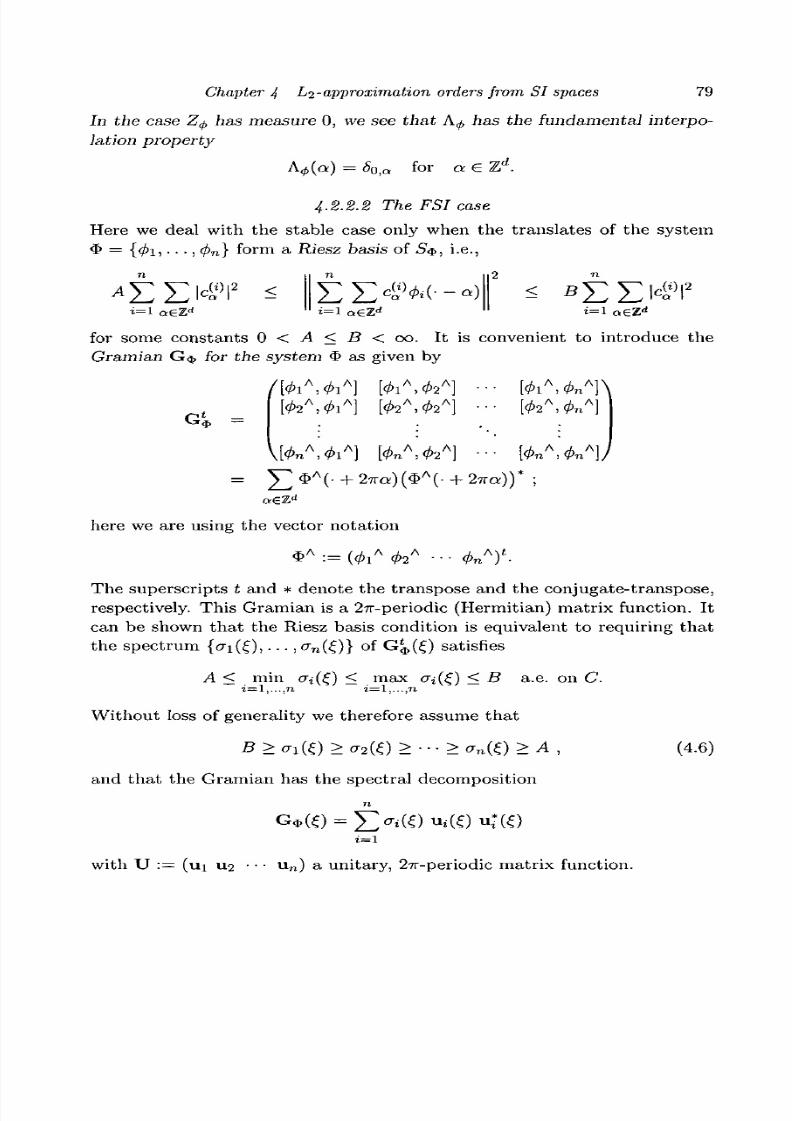
8/3/2019 Multivariate Approximation
http://slidepdf.com/reader/full/multivariate-approximation 89/296
Chapter 4 L2-approxim ation orders from SI spaces 79
In the case Z^ has measure 0, we see that A$ has the fundamental interpo-
lation property
4.2.2.2 The FSI case
Here we deal with the stable case only when the translates of the system$ = {t^j , . . . i 0 n } form a Riesz basis of S$, i.e.,
t = l
for some constants 0 < A < B < 00. It is convenient to introduce th e
Gramian G $ for the system $ as given by
G t _* =
here we are using the vector notation
The superscripts t and * denote the transpose and the conjugate-transpose,
respectively. T his Gram ian is a 27r-periodic (Herm itian) m atrix function. Itcan be shown that the Riesz basis condition is equivalent to requiring that
the spectrum {<7i(£), • • •, 0n(£)} of G$(£) satisfies
A < min <7i(£) < max <7i(£) < B a.e. on C.
Without loss of generality we therefore assume that
: • • • > M O > A , (4.6)
and that the Gramian has the spectral decomposition
with U := (ui 112 • • • u n ) a unitary, 27r-periodic matrix function.
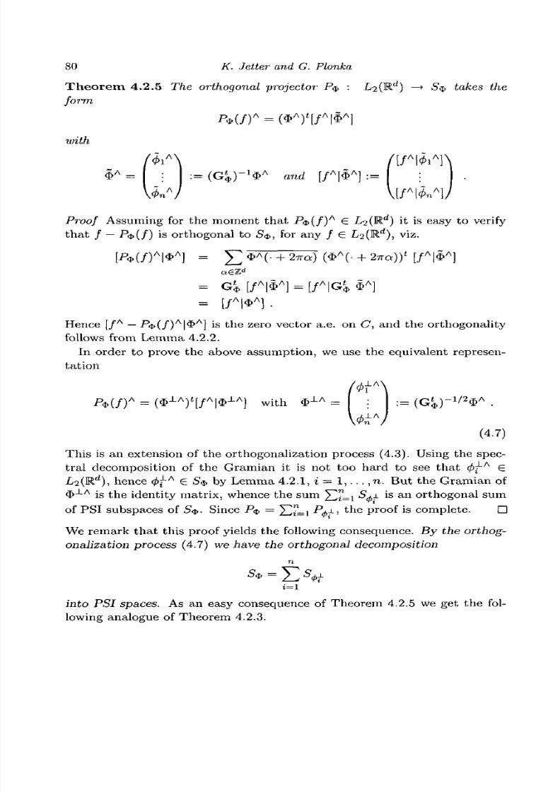
8/3/2019 Multivariate Approximation
http://slidepdf.com/reader/full/multivariate-approximation 90/296
80 K. Jetter and G. Plonka
T h e o r e m 4 . 2 . 5 The orthogonal projector P<j, : L2(Rd) —* 5 $ takes the
form
with
/ [ / A | 0 i A ]
= ( G ^ ) - X $ A and [/A
|$A
] := :
\ [ / A | 0 n A ]
Proof Assuming for the moment tha t -P$( / ) A 6 Z/2(Rd) it is easy to verify
t h a t / — P<s>(f) is orthogonal to 5$, for any / € Z/2(K d), viz.
' [/A|$
A
[/A|$
A] = [
Hence [/A — ^><f>(/)A|$A] is the zero vector a.e. on C, and the or thogona l i tyfollows from Lemma 4.2.2.
In order to prove the above assumption, we use the equivalent represen-
ta t ion
= ( $ - i A ) t [ / A | $ - L A ] with $ ± A =
(4.7)
This is an extension of the orthogonalization process (4.3). Using the spec-
tra l decom pos ition of th e G ram ian it is no t to o har d to see tha t </> -A €
L2(R d), hence <^ A 6 5$ by Lemma 4.2.1, i - 1 , . . . , n . B u t t h e G r a m i a n of
$-L A is the identi ty matrix , whence the sum X/2=i Sd>±ls a n or thogona l sum
of PSI subspaces of 5$. Since P$ = Y^i-\ P(j>±> t n e P r o ° f is com plete. •
We remark that this proof yields the following consequence. By the orthog-
onalization process (4.7) we have the orthogonal decomposition
into PSI spaces. As an easy consequence of Theorem 4.2.5 we get the fol-
lowing analogue of Theorem 4.2.3.

8/3/2019 Multivariate Approximation
http://slidepdf.com/reader/full/multivariate-approximation 91/296
Chapter I Li-approximation orders from SI spaces 81
Theorem 4.2.6 Let P$ denote the orthogonal projector onto the stable FSI
space 5$ . Then for f g L2(Rd) such that supp/
AC C, we have the error
formula
11/ -
Remark 4.2.7 We may add the useful information that the function
satisfies
where B is the Riesz constant in (4.6). Furthermore
and we arrive at the following fundamental interpolation property:
A(a) = nS0,a , a € Zd.
4-2.3 Approximation order
We first consider the PSI space generated by the famous sine function
T T S l n nxi 1A / \ I 1) l r ? £ ^ ><p[x) : = I I a n d <p (?) = XC(O — \ (4-8)
T_J KXi ^0, otherwise.
Here, by (4.2), P 0 ( / )A = f
AXc, whence
l2 r a
l /A( O I
2^
for any m 6 R + , with |£| the Euclidian norm of £ G Rd. This implies
Lemma 4.2.8 The PSI space generated by the sine function (4.8) has ap-
proximation order m, for f 6 W2l(M
d); where m is any positive real.
We next prove the important fact that the approximation order of an FSI
space is already given by the approximation order of a PSI subspace 5^, as
follows.
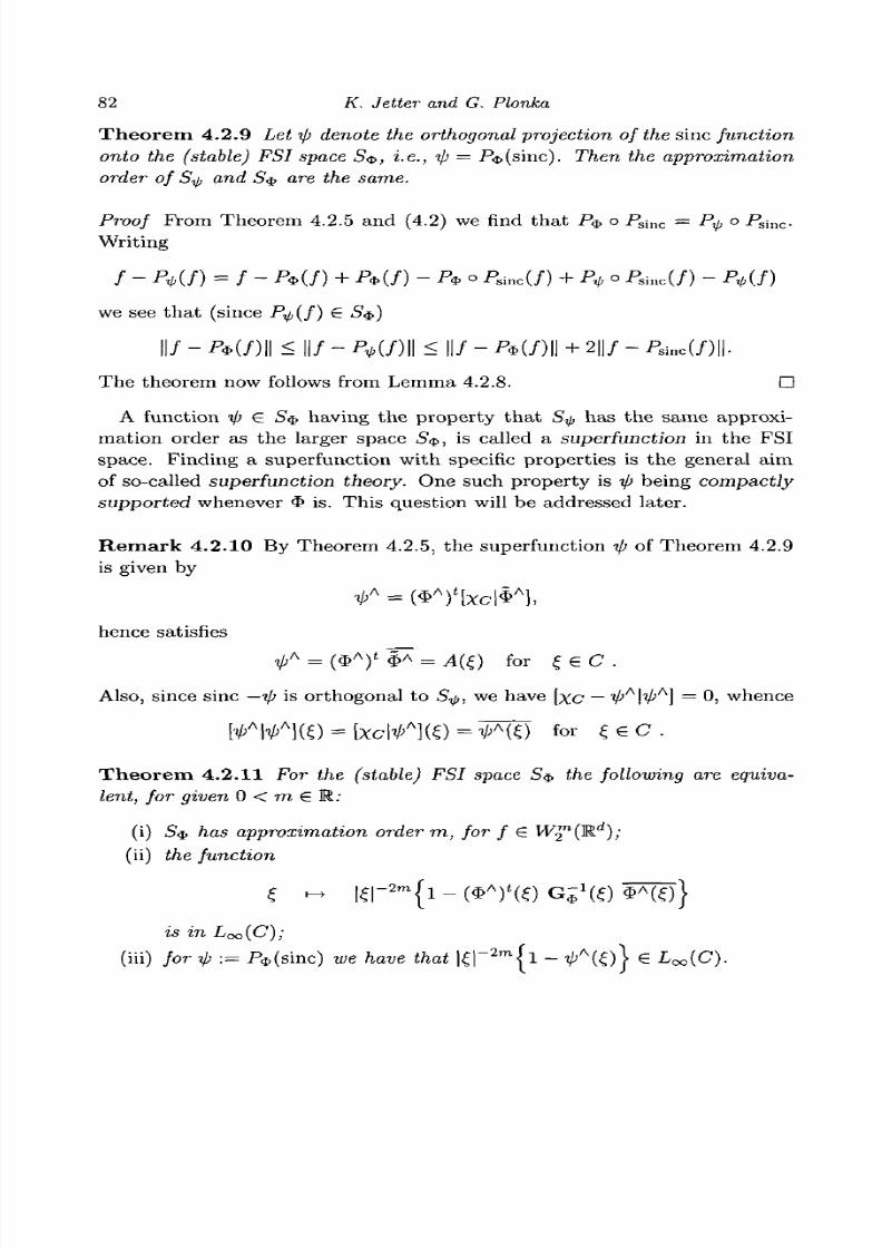
8/3/2019 Multivariate Approximation
http://slidepdf.com/reader/full/multivariate-approximation 92/296
82 K. Jetter and G. Plonka
Theorem 4.2.9 Let ip denote the orthogonal projection of the sine function
onto the (stable) FSI space 5$, i.e., ip = P$(smc). Then the approximation
order of S^ and 5$ are the same.
Proof From Theorem 4.2.5 and (4.2) we find that P$ o Psinc = P^ o Psinc .
Writing
= / - P*(f) + P*U) ~ P* ° Psinc(f) + P^ ° Psinc(/) ~
we see that (since -Pv(/) ^ ^*)
11/ - P»(/)| | < 11/ - P*(f)\\ < ||/ - P*(/)|| + 2||/ - Psinc(/)||.
The theorem now follows from Lemma 4.2.8. •
A function ip £ 5$ having the property that S^ has the same approxi-
mation order as the larger space 5$, is called a superfunction in the FSI
space. Finding a superfunction with specific properties is the general aim
of so-called superfunction theory. One such property is ip being compactly
supported whenever $ is. This question will be addressed later.
Remark 4.2.10 By Theorem 4.2.5, the superfunction ip of Theorem 4.2.9
is given by
hence satisfies
tpA
= ($A
) ' $A
= A(£) for £ € C .
Also, since sine — ip is orthogonal to Sy,, we have [xc — tpA\ip
A] = 0, whence
' U) = ?/>A(£) for f e C .
Theorem 4.2.11 For the (stable) FSI space 5$ the following are equiva-
lent, for given 0 < m € M.:
(i) S$ has approximation order m, for f € iy
(ii) the function
in
(iii) / or V := .Rj>(sinc) we /law i/iai | C|"2 m
{l -
8/3/2019 Multivariate Approximation
http://slidepdf.com/reader/full/multivariate-approximation 93/296
Chapter 4 L2-approximation orders from SI spaces 83
Proof W ith / = /1 + /2, where /1 = / A x c is the orthogonal projection of
/ onto 5Si,lc, we have
11/ - P*( /)|| < ||/i - P* (/i)|| + II/2 - P* (/2)|| < ll/i -
Moreover, for / e W2m(Rd),
\\f2f = (2n)-d f | /
A(£ ) |
2d£ < I/IS.,2-
JR d\C
The theorem now follows from Theorems 4.2.3 and 4.2.6, in view of Re-
mark 4.2.10. •
Remark 4.2.12 The second statement of this theorem is equivalent to the
order relation
l - ^ O G ^ K ) ^ ) = Om2m) a s S - O ,
see Remark 4.2.7. Also, statement (iii) of the theorem is equivalent to the
order relation
1 - VA( O
=O ( K I
2 m)
a s£ - > 0 .
4-2.3.1 The (stable) compactly supported case
We now assum e th at 5 $ is generated by com pactly supp orte d functions.
In this case , the bracket products [<AiA|0jA], i,j = l,... ,n, all have finitely
many Fourier coefficients (since the functions <j>i*<pj are compact ly suppor ted
as well); i .e. , we have identity in (4.1), and the entries of the Gramian are
all t r igonometric polynomials .
In part icular , i f G$(0) is regular , and this is certa inly true under the
Riesz basis condition assumed here, then the function A is holomorphic in a
neighborhood of the origin. Hence the order relations in Rem ark 4.2.12, at
Jeasfc for 2m £ N, can be checked by looking at the power series expansion
of 1 — A(£) at the origin.
4-2.3.2 The compactly supported PSI case
This case can be dealt with without recourse to the assumption of stability.
Here, the zero set of the trigonometric polynomial [<^A|< >A] in C has (d-
dimensional Lebesgue) measure 0, and A^ as defined in Remark 4.2.4 hasthe fundamental interpolation property. Indeed, let us set
From Theorem 4.2.3 we can deduce
8/3/2019 Multivariate Approximation
http://slidepdf.com/reader/full/multivariate-approximation 94/296
84 K. Jetter and G. Plonka
T h e o r e m 4 . 2 . 1 3 Let <fi e L2(R d) be compactly supported, and 0 < m 6
Then 5 ^ has approximation order m for f 6 W^2™(Rd) if and only if
Th is ord er relation can be expressed in an oth er equivalent way, viz. from
(4.9) we see that it is equivalent to requiring that
as f - » 0, for all 0 + a
A special case of this is
T h e o r e m 4 . 2 . 1 4 Let cf> € L2(R ) be compactly supported, and assume that
[0 A |0A](O) 7^ 0. Then for m € N the following are equivalent:
(i) S^ /ias approximation order m, for f 6 H /2™(Rd);
(ii) 4> satisfies the conditions
D p<j)A(2iTa) = 0 for0^a£Zd and | /?| < TO .
4-2.3.3 Com pactly supported superfunctionIn the case 4.2.3.1 it is interesting to search for a compactly supported
superfunc t ion . With ip as in Theorem 4.2.9, according to Remark 4.2.10,
we see that on the fundamental cube C, ip coincides with A as given in
Remark 4.2.7. Since the components of $ A are entire functions, and since
the coeffic ient functions of the Gramian G$ are tr igonometric polynomials
(wi th de te rm inan t non-vanish ing due to the Riesz bas is p rop er ty) we see th a t
A (hence tjj) is C°° in a neighborhood of the origin. Also, the representat ion
of 4>A
€ 5$ according to Lemma 4.2.1 is determined in Remark 4.2.10 as
ipA = Y,ri<Pi
A with Ti\c = 4>iA\c , i = 1 , . . .,n.t=i
From this it also follows that the 27r-periodic functions TJ are C°° in a neigh-
borhood of the origin ( in fact everywhere, according to our s trong assump-
t ions ) .
The idea is now to mimic the behavior of T/>A at the origin by a function
n
^A = £ f . 0.A (4.10)
« = 1
with trigonometric polynomials fj, in order to have ip as a compactly sup-
po rte d function. Th is can be don e, at least for integral m, by forcing the

8/3/2019 Multivariate Approximation
http://slidepdf.com/reader/full/multivariate-approximation 95/296
Chapter 4 L?-approximation orders from. SI spaces 85
trigonom etric polynomials to satisfy the interpolatory conditions
Dpn{0) = D0Ti(Q) for 0 < \(3\ < m a n d i = l,...,n.
Using Remarks 4.2.12 and 4.2.10 for ip, we see that
DptpA(0) = D pi> A{0) = <5O/3 a nd
P/3ViA(27ra) = L»/3V>A(27ra) = 0, for 0 ^ a € Zd
and \/3\ < m .
Hence Sr has approximation order m for / € W^iW 1)- We obtain
Theorem 4.2.15 Given a stable FSI space S$ with compactly supportedgenerators <t>i, • • • , (fin, the following are equivalent for m £ N:
(i) S<j) has approximation order m, for f £ W
(ii) there exists a unique function i / i £ 5 $ which has the following prop-
erties:
(a) i/5A
is of the form (4.10), where
n € s p a n { e - ^ : / 3 e Z | , \0\ < m };
(b) V>A(0) = 1 and D^A(0) = 0 for (3 SE Z^ 0 < |/3| < m;
(c) Sj; has approximation order m, for f G H /2?l(R d).
The superfunction ip of this theorem is called the canonical superfunction,
and the vector v := ( n , . . . ,fn) is sometimes referred to as the canonical
^-vector of order m.
4-2.4 Notes and extensions
4.2.4-1
Shift-invariant spaces have a long tradition in signal processing and ap-
proximation theory. As the most important and widely used examples of
generators we m ention the famous sine function (giving rise to expansions of
band-limited signals in terms of the Whittaker cardinal series, see Whittaker
(1935)), and Schoenberg's cardinal B-splines generating his cardinal B-spline
series, Schoenberg (1946). More recently, shift-invariant spaces have beenstudied quite thoroughly since they appear in Mallat's setup of multireso-
lution analysis, see Daubechies (1992), Chapter 5. In this section we have
tried to give an up-to-date discussion of the approximation orders provided
by (scaled versions of) such spaces. The main results are worked out in a
form which is perhaps not the most general, but which hopefully can be
understood without essential recourse to the original literature.

8/3/2019 Multivariate Approximation
http://slidepdf.com/reader/full/multivariate-approximation 96/296
86 K. Jetter and G. Plonka
4.24.2
This section is very much influenced by the fundamental work of de Boor,DeVore and Ron on ^-approximation orders of shift invariant spaces, (de
Boor et al. (1994a,1994b,1998)). We did not try to include the general Lp
case, for which we would like to refer to Jia's survey (Jia (1995a)) and the
references therein. Much of the original interest in approximation orders
stems from attempts to understand the approximation orders of box spline
spaces, see de Boor et al. (1993), Chapter 3, and the discussion of various
notions of approximation orders (like controlled or local approximation or-
ders, see, e.g., de Boor and Jia (1985), Halton and Light (1993), Jia andLei (1993a), Jia and Lei (1993b), Light (1991), Light and Cheney (1992).
Meanwhile, Ron and his coworkers have shown an interesting connection of
approximation orders of a PSI space generated by a refinable function to
the convergence of the corresponding subdivision scheme (Ron (1999)).
4.2.4.3
It is probably not fruitful to attribute the notion of bracket product to any
one au thor. Periodization techniques have been used for a long time in
Fourier analysis, a typical result being Poisson's summation formula which
holds true under various assumptions, and with varying interpretations of
iden tities. However, Jia and M icchelli (1991) and de Boor et al. (1994a) were
the first to use this notion in a form leading to a useful characterization of
orthogonality of PSI spaces, see de Boor et al. (1994a), Lemma 2.8. Th is
same paper contains Lemma 4.2.1 for the PSI case, while the general case is
given in de Boor et al. (1994b), Theorem 1.7. A simple proof of this result
is due to Jia (1998a), Theorem 2.1, see also Jia (1995a), Theorem 1.1.
4.2.44
The construction of the .^-projector in the stable PSI case is straightfor-
ward, and the orthogonalization process (4.3) has been used in the construc-
tion of orthonormal spline wavelets (with infinite support, but exponentially
decaying at infinity) by Battle and Lemarie (Battle (1987), Lemarie (1988)).
Much more involved is the general case of (4.4) and Theorem 4.2.3 (withthe convention (4.5) which is again due to de Boor et al. (1994a), Theo-
rems 2.9 and 2.20. In the FSI case the notion of the Gram ian was first used
by Goodm an and Lee (1993) and Goodman , Lee and Tang (1993). They
were also aware of the orthogonalization process (4.7) (see Goodman, Lee
and Tang (1993), Theorem 3.3). The representation of the ^-projector in
Theorem 4.2.5 and the error formula of Theorem 4.2.6 are again due to de
8/3/2019 Multivariate Approximation
http://slidepdf.com/reader/full/multivariate-approximation 97/296
Chapter 4 L?-approximation orders from SI spaces 87
Boor et al. (1994b), Theorem 3.9. An abstract form of the results in Sec-
tion 4.2.2.2, and in particular of Theorem 4.2.5, can be found in Aldroubi
(1996).
12.15
Section 4.2.3 closely follows the ideas and methods in de Boor et al. (1998),
with some slight modifications. The arguments are easier since we invoke
the assumption of stability. Concerning the more general (unstable) case,
we refer to the Remark stated in de Boor et al. (1998) after the proof of
Theorem 2.2.
4.2.4.6
The compactly supported PSI case as dealt with in Theorem 4.2.14 is well-
understood for polynomial spline functions. Fir st results in this direction
go back to the seminal paper of Schoenberg (1946). The condition given
in statement (ii) of the theorem (together with $>A(0) ^ 0) is nowadays
called the Strang-Fix conditions, due to their contribution in Strang and
Fix (1973). Assertions (i), (ii) of Theorem 4.2.14 are also equivalent to
the statement that algebraic polynomials of degree < m — 1 can be locallyexactly reproduced in S,/, (Jia (1998b), Theorem 2.1).
4.2.4.7
In the univariate PSI case d = 1 the following assertion can be shown.
Let <f> 6 L 2(R d) be compactly supported. If S^ has approximation order
m € N, for / G H /27l(K d), then there exists a compactly supported tempered
distribution r) such that ip = Nm * i] , with Nm the cardinal B-spline of order
m. Moreover, if s u p p ^ C [a,b], then 77 can be chosen in such a way thatsupp7; C [a, b — m]\ see Ron (1990), Proposition 3.6. A generalization of this
idea to the FSI case is treated by Plonka and Ron (2000).
4.3 Shift invariant spaces spanned by refinable functions
4-3.1 Dilation matrices and refinement equations
Refinable shift-invariant spaces are defined with recourse to a dilation matrix
M, i.e., a regular integer (d x d)-matrix satisfying
lim M~n
= 0 .n—*oo
Equivalently, all eigenvalues of M have modulus greater than 1. Given such
a matrix, a shift-invariant subspace S of L2(R d) is called M-reRnable, if
S£S = > s ( M"1- ) € 5 .
8/3/2019 Multivariate Approximation
http://slidepdf.com/reader/full/multivariate-approximation 98/296
88 K. Jetter and G. Plonka
In the l i te ra ture , the d i la t ion matr ix is often taken as M = 2 / (with I the
identi ty matrix) , but we al low here the general case .A shift- invariant space 5($) C L2(M.d) genera ted by $ = {<f>i,... , </>„} C
L2(K d) , is M-ref inable if and only if the function vector $ := (tfii,... , cj>n)1
satisfies a matrix refinement equation
$ = ^ P a $ ( M - - a ) . (4.11)
aeZd
Here the "coefficients" Pa are real or complex (n x n ) -ma t r i ce s . Th e m a t r ix -
valued sequence P = ( Pa)
oe z r f i s usually called the refinement mask. In th e
case of a single generator, (4.11) takes the scalar form
with the scalar-valued mask p = {p a)aeid-
For simplicity, we shall only consider compactly supported function vec-
tors <fr, an d we suppo se th a t t he refinem ent m ask P is finitely supported on
TLd
. T h e n $ C L i ( Ed
) n L2(Rd
), an d in the Fourier domain the refinementequa t ion reads
- ) $ A ( M " t -) (4.12)
wi th M~ l := ( M * ) " 1 and
the so-called refinement mask symbol. This symbol H is an (n x n ) - m a t r i xof tr igonometric polynomials on R d . Again, in the PSI case we get a scalar-
valued symbol which we denote by
The goa l of th is section is a charac te r iza t ion of the approximat ion order
of an M-refinable shift-invariant space S$ in t e r m s of the refinement mask
P , or i ts symbol H, or the associated subdivis ion and transfer operators (seeSection 4.3.4). It t u r n s out tha t the s t ruc tu re of the subla t t ices M Z d and
MlZ
d of Zd is im po rtan t . We have the p ar t i t ion ing
Zd = ( J (e + MZd) = ( J (e' + M*Zd) , (4.14)eSB e'Sfi'
where E and E' denote any set of represen ta t ives of the equivalence classes
8/3/2019 Multivariate Approximation
http://slidepdf.com/reader/full/multivariate-approximation 99/296
Chapter 4 L2-approximation orders from SI spaces 89
1d/MZ
d and Zd/M
lZ
d, respectively. Both E and E' contain y, = | det M\
representatives, and in a standard form we shall always take
E = M([0,l[d)nZd and E' = M l{[Q,l[d) DZd .
We also let
E0:=E\ {0} and E'o := E' \ {0}.
The following fact will be used below. Any 0 / a £ Z J has a unique
representation
a = (M t)e(e' + M tl3) , e>Q ,e'eE'0!peZ d. (4.15)
Th is can be seen as follows. Since lim^_ +oo(M ~ f)^a = 0, there is a unique
minimal integer t > 0 such that a € (M lYZd \ (Mt)
e+1Z
d. Using the
partitioning (4.14), we find the required unique representation.
4.3.1.1 The PSI case
Here refinability already implies that S$ has some approximation order.
T h e o r e m 4 .3 .1 Let 4> 6 L2(Kd) be compactly supported and M-refinable
with finitely supported refinement mask, and assume that <j>A(0) ^ 0. Then
(p satisfies the Strang-Fix conditions of order one, whence S4, has at least
approximation order one for f £
Proof Prom the scalar refinement equation
4>A = H{M-1-) 0 A (M-'-) (4.16)
we conclude that H(Q) = 1, and due to the periodicity of H we have
<pA{2nM la) = <pA(2na) , a € Zd .
From this, by an application of the Riemann-Lebesgue Lemma, <frA(2ira) =
\im k^oo4>A(2n(M t)ka) = 0 ior Q ^ a € Zd. The assertion follows from
Theorem 4.2.14. •
4.3.1.2 The FSI case
A generalization of this result depends upon the refinement equation (4.12)
at the origin. If $ A(0) / 0, then $A(0) is a right eigenvector of H(0) for the
eigenvalue 1. Consider a left eigenvector v, say, for this same eigenvalue, and
put •0A := v$ A . Then ip e 5$, and as in the previous proof ?/>A(27ra:) = 0
for 0 7^ a € Zd. In order to again apply Theorem 4.2.14, we just have to
require that ipA(Q) ^ 0. This gives
8/3/2019 Multivariate Approximation
http://slidepdf.com/reader/full/multivariate-approximation 100/296
90 K. Jetter and G. Plonka
T h e o r e m 4 . 3 . 2 Let $ C Z/2(Rd) be compactly supported and M-refinable
with finitely supported refinement mask and corresponding mask symbol H .
Assume that $ A ( 0 ) ^ O ; and that v H ( 0 ) = v for a row vector v satisfying
v $ A ( 0 ) ^ 0. Then ip e S$ given by ipA
:= v $A satisfies the Strang-Fix
conditions of order one, whence S^ and, a fortiori, 5 $ has at least approxi-
mation order one for f 6
4-3.1.3 The spectral condition on H ( 0 )
The addi t iona l assumpt ions made in th is theorem will appear la ter in a more
general form, namely when v = ( f i , . . . , fn) is a row vector of t r igonometr ic
polynomia ls and
T h e n ip 6 S$ is compact ly suppor ted (whenever $ is), an d we refer to
4.2.3.3 where we have constructed compactly supported superfunctions ip in
th is way. We say that v satisfies the spectral condition (of order 1) on H a t
the origin, if
(i) VA
(0) = v ( 0 ) $A
(0) 7^ 0 and( i i ) v ( 0 ) H ( 0 ) = v ( 0 ) .
For a s tronger vers ion of this condition, see Remark 4.3.6 below.
4-3.2 The zero condition on the mask symbol
The S t rang -F ix cond i t ions can be expressed as a zero condit ion on the
mask symbol . Th is condi t ion is sufficient for the PS I space S^, to have
approximat ion order . The condi t ion is also necessary in the s table case , and
even under an assumption weaker than s tabil i ty .
T h e o r e m 4 . 3 . 3 Let <j) £ Z/2(Rd) be compactly supported and M-refinable
with finitely supported refinement mask and corresponding mask symbol H.
Assume that </>A(0) ^ 0. For m € N we have:
(i) the zero condition of order m on the mask symbol,
D^{H{M~ t-)}(27re') = 0 for all e' € E'o and | p | < m, (4.17)
implies that S^, has approximation order m for f G W ^ R ) ;
(ii) conversely, if S$ has approximation order m for f G W ™ ( R d) , then
(4.17) holds true subject to
[4>A |0A](27rM-'e ') # 0 for any e' G E'o . (4.18)

8/3/2019 Multivariate Approximation
http://slidepdf.com/reader/full/multivariate-approximation 101/296
Chapter 4 £2-approximation orders from SI spaces 91
Proof Fir st let m = 1. In (4.16) we su bs tit ut e £ = 2-Kct with
a = e' + M' / J , e'e E', (3 e Zd, (e',/3) ± (0,0 ) ,
to obtain
(f>A(2Tra) = H(2nM~ le') <pA{2nM~ te' + 2TT/3) .
While for m = 1 (i) is always satisfied due to Theorem 4.3.1, we see th at as-
sertion (ii) follows since {<j>A(2nM~te'+2nP)}p€£d cannot be a zero sequence
for e' 6 E'o by (4.18).
For m > 1 we use induction and Leibniz' rule in (4.16),
-)} ^ " " { ^ ( M - ' - ) } , (4.19)
with I7I < m + 1 . In the case of statemen t (i) we see th at the zero condition of
order m + 1 immediately verifies the Strang-F ix conditions D y4>A(2na) = 0
in the following situations:
|7 | < m and 0 / a 6 Zd (via Theorem 4.2.14) ;
| 7 | = m and a = e' + M'/3, e' e E'o , (3 e Zd .
The first situation is the induction assumption. For |7 | = m and 0 / a g Z1*
as in (4.15) with I > 0, equation (4.19) reduces to
|7'I=|7|
for some constants cy 7 , and a simple induction argument with respect to (
shows th at the full Stra ng-Fix conditions of order m + 1 are satisfied. Thu s
£4, has approximation order m + 1 . In case of statement (ii), (p satisfies the
Strang -Fix conditions of order m + 1 , and due to the induction hypothesis,
the symbol satisfies the zero conditions of order m. Hence (4.19) yields, for|7 | = TO, e' € E'o, and any /? £ Zd,
0 = D~i4>A(2n(e' + M lp)) = D'y{H{M-t-)}(2ne') (f>A(2nM- te' + 2TT/3) .
Due to our assumption (4.18), this yields an additional order in the zero
condition for the mask symbol. •
8/3/2019 Multivariate Approximation
http://slidepdf.com/reader/full/multivariate-approximation 102/296
92 K. Jetter and G. Plonka
Remark 4.3.4 The zero condition on the mask symbol (4.17) is actually
equivalent to
{D 'lH}(2nM- te') = 0 for all e' € E'o and \fi\ < m . (4.20)
In the univariate case d = 1, the refinement equation is of the form
for some integer k > 2. Here this condition simplifies to
j ± \ = 0 , j = 1, • • • , k - 1, M = 0 , . . . , m - 1.
Since H is a trigonometric polynomial the zeros can be factored out as
where G is another trigonometric polynomial satisfying G(0) = 1.
4.3.2.1 Condition (Zm) and the FSI case
Th e above Theorem 4.3.3 is a special case of the theorem to follow. We
say that the matrix symbol H satisfies condition (Zm) if there exists a row
vector
v = ( f i , . . . ,f n)
of trigonometric polynomials for which(a) v satisfies the spectral condition 4.3.1.3 on H at the origin and
(b) D»{vIi(M-l-)}(2ne') = 0 for |/u| < m and e' G E'o.
Theorem 4.3.5 Let $ C Z/2(Kd) be compactly supported and M -refinable
with finitely supported refinement mask and corresponding mask symbol H .
Assume that $A(0 ) 7 0. Then for m £ N we have:
(i) if H satisfies condition (Zm), then S$ has approximation order mfor f 6 W?(R d);
(ii) conversely, if S$ /ias approximation order m for f 6 ^ " ( R ' 2 ) , and
i/ i/ie Gramian G$ is regular at £ = 2nM~ le' for any e' € £', i/ien
H satisfies cond ition (Zm).
It should be noted that the condition on the regularity of the Gramian is

8/3/2019 Multivariate Approximation
http://slidepdf.com/reader/full/multivariate-approximation 103/296
Chapter 4 L2-approximation orders from SI spaces 93
equivalent to the fact that the sequences
sue linearly independent.
Proof We can follow the proof of Theorem 4.3.3 with the same notation as
in 4.3.1.3. In particular, let %j)h
:= v $ A . Due to the refinement equation we
have
i> A{2na) = v(0) H(2nM-te') $ A (27rAr 'e ' + 2TT/3) (4.21)
for any a = e' + M l@ € Zd, and the induction procedure will use Leibniz'rule in the form
For (i) the induction is based on Theorem 4.3.2 (case m = 1), and the
induction step of the above proof extends almost word for word.
For (ii) we first consider the stronger assumption that the Gramian is
everywhere regular. Then according to Theorem 4.2.15 we can find v =( f i , . . . , fn) such that ipA = v $ A satisfies the Strang-Fix condition of order
m. In particular, the S trang-F ix conditions of order 1 already show th at
•0A(O) / 0 and
v(0) H(0) $A(27ra) = v(0) $A(27ra)
for all a G Zrf by putting e' = 0 in (4.21). Hence v satisfies the spectral
condition on H (0 ) due to the regularity of G $( 0) . The induction step is
now analogous to the earlier one.In order to see (ii) with the weaker assumptions, it should be emphasized
that Remark 4.2.10 holds true in a neighborhood of the origin as long as the
Gramian is regular there. In this way, the construction of the superfunction
in 4.2.3.3 can also be performed in this neighborhood. D
Remark 4.3.6 In the statement of Theorem 4.3.5, the row vector v can be
chosen so that its components are linear combinations of the exponentials
e~ia< with a € Z+ and \a\ < m ,
and moreover such that, besides the zero condition (Z m), the spectral con-dition of order m,
(4.22)
is satisfied for \fi\ < m.

8/3/2019 Multivariate Approximation
http://slidepdf.com/reader/full/multivariate-approximation 104/296
94 K. Jetter and G. Plonka
Remark 4.3.7 Condit ion (Z m) can be simplified in the univariate case
d — 1. It then implies a matrix factorization of the refinement mask symbol
H. Here equation (4.11) reads
aeZ
for some integer k > 2. It can be shown that there exists a trigonometric
polynomial matrix A such that
where G is another trigonometric polynomial matrix. Moreover, the factor-
ization matrix A necessarily satisfies the following two conditions:
(a) { D ^ d e t A)}(0) = 0 for |/x| < m;
(b) if ip defined by ip A : = v $ A is a superfunction (i.e., Sy, has approxi-
mation order TO) {D^(vA)}(0) = 0 for \fi\ < m.
Furthermore, setting * A ( | ) := (i£,)m MO'1 * A (0> w e obtain
with G the trigonometric polynomial matrix occurring in the above factor-
ization of H. Thus * is a compactly supported refinable distribution vector
with refinement mask symbol G.
4-3.3 The sum rules
The zero condition on the mask symbol can be given in an equivalent form.
Here the group structure of E := Zd/MZ
d enters the discussion. It is well-
known that the dual group is given by EA = 2Tr(M~ tZd/Z d), hence for the
Fourier matrix
* M ! = ( e JeeE,e'eE'
we have
F».r F * — T (d 931
]faM\bMtM
- '[ }
i.e., the matrix is unitary up to the given factor. A simple corollary of this
is
Lemma 4.3.8 For a trigonometric polynomial h(£) = J2eeB ^ e le
8/3/2019 Multivariate Approximation
http://slidepdf.com/reader/full/multivariate-approximation 105/296
Chapter 4 L2-approximation orders from SI spaces 95
following are equivalent:
(i) h(2irM-te t) = 0 for all e' e E'o;(ii) be = b0 for all e G E.
Proof Condition (i) is equivalent to the fact that the vector {be)e€E is
orthogonal to all columns of the Fourier matrix except the first one, and
this property is equivalent to the vector being a multiple of the first column
of the Fourier matrix . •
In the PSI case this can be applied to the scalar-valued mask symbol Hin the following way. Given any algebraic polynomial q and corresponding
differential operator q(iD), then
Rearranging the sum in terms of a = e + My and inserting the dual lattice
gives a • 2nM~ te' = e • 2irM~ te' (modulo 27r), whence
=
Combining this with the above lemma and with (4.17) yields the following
sum rules of order m:
Theorem 4.3.9 In the PSI case the zero condition (4.17) of order m on
the mask sym bol H is equ ivalent to the fact that the mask p satisfies
9(e + Mi) = Y, PM-, Q{My) , e £ E , (4.24)
for any algebraic polynomial q of degree less than m.
In part icular we observe that for <f> satisfying </>A(0) ^ 0 th e sum ru le of
order one,
] T Pe+Mj = J2 PM- , . e e E ,
is sufficient for S^ to have approximation order 1. The converse holds true
subject to the additional condition in Theorem 4.3.3 (ii).
Turning to the FSI case, we note that Theorem 4.3.9 is a special case
of the following statement (when dealing with the scalar case and putting
va = Sa):
8/3/2019 Multivariate Approximation
http://slidepdf.com/reader/full/multivariate-approximation 106/296
96 K. Jetter and G. Plonka
Theorem 4.3 .10 In the stable FSI case the zero condition (Zm) on the row
vector vH ( M ~ ' - ) , with v(£) = ]Caez d V « e ~ r a^ a row v^tor of trigonomet-
ric polynomials, is equivalent to the fact that the mask P satisfies the sum
rules
J2 E vt~a Ve+Mo q{e + My)
= E E V 7 - C T P M C T < ? ( M 7 ) , e € E , (4.25)
cre1d 76Z d
for any algebraic polynomial q of degree less than m.
Proof We have
a€Zd
Thus with a = e + My, e' 6 E', and q any algebraic polynomial as before,
q{iD){v H(M-t-)}(2ne')
E E -P-M 7 , (M-e + 7 +
Applying Lemma 4.3.8, the zero condition on the vector vH(M~ f-), i.e.,
(Z m )(b) in 4.3.2.1, is now equivalent to the fact that the expression within
the outer brackets does not depend upon e for any polynomial q of degree
less tha n in. Substituting q(M~
1
-) by q we arrive at the required sum rules.•
In particular, the sum rules of order 1 are satisfied if there exists a row
vector vo £ Kd such that
v 0 ^ Pe+Ma = v 0 ^2 PM, , for all e e E .
4-3-4 The subdivision operator and the transfer operator
In this section we consider two linear operators which come with the refine-
ment mask P in (4.11). These operators have been shown to be excellent
tools for the characterization of refinable function vectors.
For a given (complex) mask P = (Pa)«6Z d °f ("• x n)-matrices, the subdiv-
ision operator Sp is the linear operator on the sequence space X = (£(Zd))n

8/3/2019 Multivariate Approximation
http://slidepdf.com/reader/full/multivariate-approximation 107/296
Chapter 4 £2-approximation orders from SI spaces 97
defined by
(SPb)a := J2 K-w b/3 , a e Zd
. (4.26)
Here, b = (h a)aej,d e (^(2d))*\ '-e-; b is a vector of (complex-valued)
sequences indexed by Z d . Restricting the subdivision operator to the case
of sequences which are square summable, i.e., | |b | |2 := Y2aeZd^'o^'a < 00, or
b 6 (£2(2^))" for short, we have the vector-valued Fourier series
b A (0 := £ bQ eio
< ,
a€l.d
and (4.26) leads to
(Spb)A ( O = | d e t M | H ( O * b A ( M ' O
with the mask symbol H as in (4.13).
The transfer operator Tp (sometimes also called the transition operator)
associated with the mask P is the linear operator operating on (£o(Zd))n C
[C(Zd))n, the subspaee of compactly supported vector-valued sequences de-
fined by
(T Pd)Q := £ P M a _ ^ dp, a € i \ d €
This definition naturally extends to (£2(2^))™ due to the compact support
of the matrix mask, and the Fourier series of the image vector sequence is
given by
(T Pd)A (O = J^ H ( M - ^ + 27re')) d A ( M - '( £ + 27re')). (4.27)e'GE'
In the case of a scalar-valued mask p = (p a)aezd ^he linear operators aresimply
(S pc)a =
(T pd)a =
For c,d£ ^2(Zd) we observe that
(S pc)A( £ ) = | d e t M |H( Oc A ( M t O and
e'£E'
8/3/2019 Multivariate Approximation
http://slidepdf.com/reader/full/multivariate-approximation 108/296
98 K. Jetter and G. Plonka
It is this version of the transfer operator dA
\—> (Tpd)A
in the Fourier domain
and operating on (Z,2(C)) which frequently appears in the literature.
There is a close connection between the two operators. When operating
on {ii{Jjd^)
nconsidered as a Hilbert space with scalar product
(b | d> := £ b ^ d Q , (4.28)
it is easy to see that the adjoint operator Sp defined by (Spb | d) = (b | Spd)
is given by
S*Pd=(TP(d-)y (4.29)
with d"Q := d_ a denoting the reflection of a sequence. From this it is clear
that, considered as operators on X = (£2(Zd))
n, the spectra crx(Sp) and
<Jx{Tp) are related through complex conjugation, i.e.,
The situation is slightly more involved if we look at eigenvalues of the
operators. Here it is opportune to consider (4.28) as a sesquilinear form on
the dual pairing
X x X' := (e{Zd))nx (<?0(Z d))n
(the canonical bilinear form being (4.28) with the superscript "*" replaced
by "£"). Then the formal extension of (4.29) is still true, and the following
theorem can be shown along the lines of Theorem 5.1 in J ia (1998b).
Theorem 4.3.11 Considered as an operator on (£o(Zd))
n, Tp has only
finitely many nonzero eigenvalues. In particular a is an eigenvalue of Tp
if and only if a is an eigenvalue of Sp, the latter being considered as an
operator on
It is possible to characterize the approximation order of S(<&) in terms
of properties of invariance of the subdivision and the transfer operator. A
linear subspace Y C (^o(^d))" is called Tp-invariant if
d e Y =>• TpdeY ,
and Sp-invariant subspaces Z C (^(Zd))
nare defined analogously.
4.3.4.1 The PSI case
For given m € N we put
Vm := {d € 4(Zd) ; D^d
A(0) = 0 for all n € 1% with \p\ < m). (4.30)

8/3/2019 Multivariate Approximation
http://slidepdf.com/reader/full/multivariate-approximation 109/296
Chapter 4 L2-approximation orders from SI spaces 99
Since dA
is a trigonometric polynomial, the derivatives at the origin are well-
defined. These zero conditions at the origin are moment conditions for the
sequence d. Indeed since c(A(£) = ^a&iddae
ia^, we have
(-iDYdA(0) = 0 ^
whence
Lemma 4.3.12 The following are equivalent for ra£N and d £ &Q
(i) deVm;
(ii) ^ da q(a) = 0 for any algebraic polynomial q of degree less than
We are now ready to present the abovementioned invariance properties
which imply an approximation order result, in view of Theorem 4.3.3. By
a slight misuse of notation we identify the polynomial space Pm-\ (i.e.,polynomials of degree less than m) with the sequence space of polynomials
of order TO, evaluated at Zd, namely,
{(<?(«))„«<; «ePm_i} c
Theorem 4.3.13 Let p € IQ{1T) be a finitely supported mask with corre-
sponding scalar mask symbol H. Then the following assertions are equivalent
for m € N:
(i) Vm C io(Zd) is invariant under the transfer operator Tp;
(ii) Pm-\ is invariant under the subdivision operator Sp;
(iii) H satisfies the zero condition (4.17) of order m;
(iv) p satisfies the sum rules (4.24) of order m.
The equivalence of (i) and (iii) is obvious from the Fourier transform ex-
pression of the transfer operator,
The equivalence of (iii) and (iv) was established in Theorem 4.3.9. The
implications (i) => (ii) => (iv) can be taken from Jia (1998b), Theorem 5.2.

8/3/2019 Multivariate Approximation
http://slidepdf.com/reader/full/multivariate-approximation 110/296
100 K. letter and G. Plonka
4.3.4.2 The FSI case
Theorem 4.3.13 is a special case of the following statements. For a givenrow vector
v(£) = $ > « * e ~ t o * (4.31)aeZd
of trigonometric polynomials we extend the definition in (4.30) to
y m (v) := {d 6 ( 4 ( Z d ) ) n ; D '1{vd
A}(0) = 0 for all fi € Z
d+ with |/J| < m } .
As previously in the PSI case, the zero conditions for v d
A
at the origin aremoment conditions for the "convolved" series v * d~£ £o(Zd) given by
(v * d~)Q := ^ va-pd~p = ^2 va+pdp , a£Zd.
Note that dA(£) = ^aezddae lae- is a column vector of trigonometric poly-
nomials. Therefore Lemma 4.3.12 gives
Lemma 4.3.14 Given the row vector v in (4.31), the following are equiva-lent for men and d € (e o(Z d))n:
(i) deVm(v);
(ii) v*d-eVm;
( i u) £ 7 6 Z d ( £/36Zd v7+/3
d/3) 9(7) = 0 for any algebraic polynomial q ofdegree less than m.
Theorem 4.3.15 Let P be a finitely supported (n x n)-matrix mask with
mask symbol H. Let v be a row vector (4.31) of trigonometric polynomialssuch that the spectral conditions (4.22) of order m € N are satisfied. Then
the following assertions are equivalent:
(i) Vm(v) is invariant under the transfer operator Tp;
(ii) H satisfies condition (Zm) with v.
Proof For d G V ^ v ) we have, using (4.22),
{v H(M-f- )}(0) D'i-/{d A(M
= 5 ' ' { ( v d A ) ( M - ' - ) } ( 0 ) = 0 , \fi\<m.
8/3/2019 Multivariate Approximation
http://slidepdf.com/reader/full/multivariate-approximation 111/296
Chap ter 4 L2-approximation orders from SI spaces 101
On the other hand, by (4.27), for any d e (eo(Z d))n,
Z)"{v(r Pd)
A
}(0) =
^"{&*{M~l{• + 27re'))}(0).
e'eE' v<ii
Since Tpd is flnitely supported whenever d is, statement (i) is equivalent to
the fact that
E E ( ^W{ vH( M - t( - + 27re'))}(0) ^ - /{ d A (M " t(-+ 27re'))}(0)
= 0 for any d 6 Vm(v) and \fi\ < m .
It is not hard to see that this is equivalent to condition (Z m). •
As a corollary of this theorem we have
Theorem 4.3.16 In the stable FSI case, any of the statements in Theo-
rem 4.3.15 can be replaced by the sum rules of Theorem 4.3.10. Here the
appropriate form of the spectral conditions (4.22) is
det M\ E E
v- v - P M
- <?(M 7) = Ev* 9 (
Q) (
4-32)
for any polynomial q of degree less than m.
In order to relate the conditions in Theorem 4.3.15 to an invariance prop-
erty of the subdivision operator we let
n(z
d
) c i{z
d
)denote the space of all sequences which increase at most polynomially at
infinity. In addition, we put
W m(v) := | b € ( n ( Z d ) ) n ; (b I d) = 0 for all d € K m (v)} .
Theorem 4.3.17 In the stable FSI case, any of the statements in Theo-
rem 4.3.15 can be replaced by either of the following equivalent conditions:
(i) W m(v) is invariant under the subdivision operator Sp;
(ii) P satisfies the sum rules (4.25) with v.
Proof (ii) = > (i): Using Theorem 4.3.10 and Theorem 4.3.15 we see th at
(ii) implies the invariance property of Tp. Therefore, by (4.29), Vm(v) is
also invariant under the operator Sp. Due to the finite support of the mask
8/3/2019 Multivariate Approximation
http://slidepdf.com/reader/full/multivariate-approximation 112/296
102 K. Jetter and G. Plonka
P we also have
b e (n(zd))n => sPb e (n(zd))n .
Therefore, given b € W m(v) we obtain
(S Pb | d) = (b | S*Pd) = 0 ,
for any d e V ^ v ) , whence Spb g W m (v) .
(ii) <= (i) : By Lemma 4.3.14, d G Vm{\) if and only if
for all algebraic polynomials q of degree less than m. Setting.0
q{8 - a ) = J2 »•/»(«)(-<*)"
the spectral conditions (4.32) yield
0= E E
= |detM| X) ( E E v - r - / » P ^^(M7)) ^(-a)"da. (4.33)
Now let g be any algebraic polynomial of degree less than m. Then thevector sequence b = b(q) given by
, a G Zd,
is an element of (Jl(Zd))n, since (vQ)Q£Z d is compactly supported. It is
contained in W m (v) since for all d € V^j(v), using Lemma 4.3.14,
From our assumption (i) we conclude that Spb € W m(v) as well, i.e., for

8/3/2019 Multivariate Approximation
http://slidepdf.com/reader/full/multivariate-approximation 113/296
Chapter 4 L2-approximation orders from SI spaces 103
any d € Vm(v):
0 = (5Pb|d)= £(Spb)*da
= E ( Ep«-
EEquivalently, putting
we have
«=E E (for all d £ Vm(v). Comparing this with (4.33) shows that the expression
within the outer brackets must be independent of a, for any polynomial q
of degree less than m. Whence the sum rules (4.25) of order m hold true,
as we desired. D
4-3.5 Notes and extensions
4.3.5.1
A stable, compactly supported M-refinable function or function vector gen-
erates a multiresolution analysis for L2(Rd), hence allows for a (now) stan-
dard construction of a wavelet basis.
The dilation matrix M in the matrix refinement equation (4.11) is often
chosen as M = 21, with / the dx d unit matrix. For this special case, refin-
able functions can be obtained from tensor products of refinable univariatefunctions <pi, say, as
All results on univariate refinable functions can be simply transfered to the
8/3/2019 Multivariate Approximation
http://slidepdf.com/reader/full/multivariate-approximation 114/296
104 K. Jetter and G. Plonka
multivariate situation. Th e corresponding wavelet basis then requires 2d— 1
different generating wavelets.
In general, dilation matrices M of smallest possible determinant are of
special interest, since the construction of a corresponding wavelet basis con-
sists of |detM| — 1 wavelets (or multiwavelets). If M is not a diagonal
matrix, these wavelets are called non-separable, see Cohen and Daubechies
(1993). An important instant of this is the bivariate construction based on
M ={l -l
For example, the so-called Zwart-Powell element is refinable with respect to
the first matrix. See de Boor et al. (1993), Chapter 7 for more information
on approximation orders and subdivision of so-called box splines.
4.3.5.2
Considering the refinement equation (4.12) in the Fourier domain, it follows
that
(i) $A(0) is either a right eigenvector of H(0) with corresponding eigen-value 1, or
(ii) $A(0) is the zero vector.
The latter case is not of real interest since then $ can be considered as
a derivative of an M-refinable function vector $ with I>A 7 0. Thus the
assertion that H(0) has an eigenvalue 1 is the fundamental condition, and
the spectral condition on H(0) in Section 4.3.1.3 just ensures that v(0)
and $(0) are non-orthogonal left and right eigenvectors of H(0) to thiseigenvalue. Th e condition of these eigenvectors being non-orthogonal is
clearly vacuous if 1 is a simple eigenvalue.
Moreover, if $ C L2{Rd) generates a stable, M-refinable FSI-space, then
the spectral radius of H(0) necessarily equals 1, with 1 being a simple eigen-
value and the only eigenvalue of absolute value 1, see e.g. Dahmen and
Micchelli (1997).
4.3.5.3
For a given refinement mask the refinement equation (4.11) can be inter-
pre ted as a functional equation for <&. In the Fourier domain th e solution
vector can be formally written as
= limL—>oo -
i

8/3/2019 Multivariate Approximation
http://slidepdf.com/reader/full/multivariate-approximation 115/296
Chapter 4 L2-approximation orders from SI spaces 105
where r is a right eigenvector of H(0) to the eigenvalue 1. In particular it
follows that $A
(0) = r.
The convergence of the infinite product (in the sense of uniform conver-
gence on compact sets) is ensured if the spectral radius of H(0) is 1, and if
there are no further eigenvalues of H(0) on the unit circle. In this case a
non-degenerate eigenvalue 1 defines a solution vector $A
. If the eigenvalue
1 is simple (see 4.3.5.2), then this solution vector $ is unique.
4-3.5.4
Section 4.3 often refers to work of Jia on approximation properties of mul-
tivariate wavelets. In his paper (Jia (1998b)) the PSI case was completely
settled for general dilation matrices; see also the following remarks. The
proof of Theorem 4.3.1 is a trivial extension of the proof of Jia and Mic-
chelli (1991), Theorem 2.4.
4.3.5.5
In the univariate FSI case, d = 1, the zero condition (Zm) and its conse-
quence for the approximation order of 5<t> have been considered by Heil et
al. (1996) and Plonka (1995a,1997) in the Fourier domain, while Lian (1995)
has given conditions in the time domain.
In particular, in Plonka (1997) it is shown that the approximation order
induces a matrix factorization of the symbol H; see Remark 4.3.7. Sub-
sequently Micchelli and Sauer (1997) observed an analogous factorization
property for the representing matrix of the subdivision operator. Unfortu-
nately, for d > 1 the zero conditions on the mask symbols (4.17) and (4.20)
do not lead a priori to a factorization of the symbols.
The multivariate FSI case with arbitrary dilation matrices is, for example,
treated in Cabrelli et al. (1998). The observed conditions relate to the sum
rules of Theorem 4.3.10.
4.3.5.6
The generalized discrete Fourier transform matrix Fj< and its property in
(4.23) of being unitary are well-known, see e.g. Chui and Li (1994). These
properties have been used by Jia (1998b) to derive the sum rules as in
Theorem 4.3.9.
4.3.5.7
While the notion of subdivision operator Sp (for general dilation matrices)
has been coined by Cavaretta et al. (1991), the set-up for the transfer or
transition operator is often altered in the literature. We prefer here to say
8/3/2019 Multivariate Approximation
http://slidepdf.com/reader/full/multivariate-approximation 116/296
106 K. Jetter and G. Plonka
that Tp is (essentially, i.e., modulo reflection) the adjoint of Sp. In this
way, Theorem 4.3.13 dealing with the PSI case is identical with Jia (1998b),
Theorem 5.2. As far as the FSI case is considered our results are new.
It should be noted that for the PSI case and M = 21, the invariance
of Pm-\ under the subdivision operator Sp is equivalent to the property
that polynomials of order less than m can be reproduced from multi-integer
translates of 0. A result along these lines is already contained in Cavaretta
et al. (1991).
4.3.5.8
The symmetrized form of the transfer operator (in the Fourier domain) is
given by TpA operating on (n x n)-matrices C of trigonometric polynomials
as follows,
V) H(M-*( f + 2ire')) C(M"*(£ + 2ne')) H(M ~* (^ + 27re'))*. (4.34)
For M = 21, Shen (1998), Theorem 3.8 has shown that the stability of S$
is equivalent to the following condition: the operator TAhas spectral radius
1, with 1 being a simple eigenvalue and all other eigenvalues lying strictly
inside the unit circle. Moreover, the eigenmatrix of fp A corresponding to
the eigenvalue 1 is nonsingular on the d-dimensional torus. We conjecture
that this equivalence is also true for arbitrary dilation matrices.
4.3.5.9
When considering the dilation matrix M = 21, the connection between
properties of the subdivision operator Sp and the approximation order m
provided by the FSI-space 5$ can be simply stated as follows: the stable
FSI space 5$ has approximation order m, for f € W ™ ^ ^ ) , if and only if
there exists a nontrivial vector q of polynomial sequences q\, • • • , qn £ P-m-i
such that
Spq = 2"('™-1) q.
In particular Sp necessarily has the eigenvalues 2~k for k = 0 , . . . , m — 1.
This result can be generalized to distribution vectors $ which do not
satisfy any conditions of linear independence (see Jia et al. (1997), Theo-
rem 3.1).
8/3/2019 Multivariate Approximation
http://slidepdf.com/reader/full/multivariate-approximation 117/296
Chapter 4 L2-approx imation orders from SI spaces 107
R e f e r e n c e s
Aldroubi, A. (1996). Oblique projections in atomic spaces. Proc. Arner. Math.Soc, 124, 2051-2060.Battle, G. (1987). A block spin construction of ondelettes. Part I: Lemarie
functions. Comm. Math. Phys., 110, 601-615.Blu, T. and Unser, M. (1999). Approximation error for quasi-interpolators and
(multi-) wavelet expansions. Appl. Comput. Harmonic Anal., 6, 219-251.Boor, C. de (1987). The polynomials in the linear span of integer translates of a
compactly supported function. Constr. Approx., 3, 199-208.Boor, C. de (1990). Quasiinterpolants and approximation order of multivariate
splines. In Computation of Curves and Surfaces, ed. W. Dahmen, M. Gasca
and C.A. Micchelli, pp. 313-345. Kluwer Academic Publ., Dordrecht.Boor, C. de (1993). Approximation order without quasi-interpolants. InApproximation Theory VII, ed. E.W. Cheney, C.K. Chui and L.L.Schumaker, pp. 1-18. Academic Press, New York.
Boor, C. de, DeVore, R.A. and Ron, A. (1994a). Approximation fromshift-invariant subspaces of L2(Rd). Trans. Amer. Math. Soc, 341, 787-806.
Boor, C. de, DeVore, R.A. and Ron, A. (1994b). The structure of finitelygenerated shift-invariant spaces in L2(R d). J- Fund. Anal, 119, 37-78.
Boor, C. de, DeVore, R.A. and Ron, A. (1998). Approximation orders of FSIspaces in L2(R d). Constr. Approx ., 14, 411-427.
Boor, C. de and Fix, G. (1973). Spline approximation by quasi-interpolants. J.Approx. Theory, 8, 19-45.Boor, C. de, Hollig, K. and Riemenschneider, S.D. (1993). Box Splines.
Springer-Verlag, New York.Boor, C. de and Jia, R.Q. (1985). Controlled approximation and a characterization
of local approximation order. Proc. Arner. Math. Soc, 95 , 547—553.Boor, C. de and Jia, R.Q. (1993). A sharp upper bound on the approximation
order of smooth bivariate pp functions. J. Approx. Theory, 72, 24-33.Boor, C. de and Ron, A. (1992). Fourier analysis of approximation power of
principal shift-invariant spaces. Constr. Approx., 8, 427-462.
Burchard, H.G. and Lei, J.J. (1995). Coordinate order of approximation byfunctional-based approximation operators. J. Approx. Theory, 82, 240-256.Cabrelli, C , Heil, C. and M olter, U. (1998). Accuracy of lattice t ran slates of
several multidimensional refinable functions. J. Approx. Theory, 95, 5-52.Cavaretta, A.S., Dahmen, W. and Micchelli, C.A. (1991). Stationary Subdivision.
Memoirs of the Amer. Math. Soc., Vol. 93, Providence.Chui, C.K. (1988). Multivariate Splines. CBMS-NSF Reg. Conf. Series in Applied
Math., Vol. 54, SIAM, Philadelphia.Chui, C.K. and Diamond, H. (1987). A natural formulation of quasi-interpolation
by multivariate splines. Proc. Amer. Math. Soc, 99, 643-646.
Chui, C.K., Jetter, K. and Stockier, J. (1994). Wavelets and frames on thefour-directional mesh. In Wavelets: Theory, Algorithms, and Applications, ed .C.K. Chui, L. Montefusco and L. Puccio, pp. 213-230. Academic Press, NewYork.
Chui, C.K., Jetter, K. and Ward, J.D. (1987). Cardinal interpolation bymultivariate splines. Math. Comp., 48, 711-724.
Chui, C.K. and Li, C. (1994). A general framework of multivariate wavelets withduals. Appl. Comput. Harmonic Anal., 1, 368-390.
8/3/2019 Multivariate Approximation
http://slidepdf.com/reader/full/multivariate-approximation 118/296
108 K. Jetter and G. Plonka
Cohen, A. and Daubechies, I. (1993). Non-separable bidimensional wavelet bases.Revista Mathemdtica Iberoamericana, 9, 51-137.
Cohen, A., Daubechies, I. and Feauveau, J. (1992). Biorthogonal basis ofcompactly supported wavelets. Comm. Pure and Appl. Math., 45, 485-560.
Dahmen, W. and Micchelli, C.A. (1983). Translates of multivariate splines. LinearAlgebra Appl, 52(3) , 217-234.
Dahmen, W. and Micchelli, C.A. (1984). On the approximation order from certainmu ltivariate splines. J. Austral. Math. Soc. Ser. B, 26, 233-246.
Dahmen, W. and Micchelli, C.A. (1997). Biorthogonal wavelet expansions.Constr. Approx., 13, 293-328.
Daubechies, I. (1992). Ten Lectures on Wavelets. CBMS-NSF Reg. Conf. Series inApplied Math., Vol. 61, SIAM, Philadelphia.
DeVore, R.A. and Lorentz, G.G. (1993). Constructive Approximation.Springer-Verlag, Berlin.
Dyn, N. (1989). Interpolation and approximation by radial and related functions.In Approximation Theory VI, ed. C.K. Chui, L.L. Schumaker and J.D. Ward,pp. 211-234. Academic Press, New York.
Dyn, N., Jackson, I.R.H., Levin, D. and Ron, A. (1992). On multivariateapproximation by the integer translates of a basis function. Israel J. Math.,78, 95-130.
Goodman, T. and Lee, S. (1993). Wavelets of multiplicity r. Trans. Amer. M ath.Soc, 342, 307-324.
Goodman, T., Lee, S. and Tang, W.S. (1993). Wavelets in wandering subspaces.Trans. Amer. Math. Soc, 338, 639-654.
Goodman, T., Micchelli, C.A. and Ward, J.D. (1994). Spectral radius formulas forsubdivision operators. In Recent Advances in Wavelet Analysis, ed .L.L. Schumaker and G. Webb, pp. 335-360. Academic Press, New York.
Halton, E.J. and Light, W.A. (1993). On local and controlled approximationorder. J. Approx. Theory, 72, 268-277.
Han, B. and Jia, R.Q. (1998). Multivariate refinement equations and convergenceof subdivision schemes. SIAM J. Math. Anal., 29, 1177-1199.
Heil, C , Strang, G. and Strela, V. (1996). Approxim ation by transla tes of
refinable functions. Numer. Math., 73 , 75-94.Jetter, K. (1993). Multivariate approximation from the cardinal interpolation
point of view. In Approximation Theory VII, ed. E.W. Cheney, C.K. Chuiand L.L. Schumaker, pp. 131-161. Academic Press, New York.
Jetter, K. and Zhou, D.X. (1995a). Order of linear approximation fromshift-invariant spaces. Constr. Approx., 11, 423-438.
Jetter, K. and Zhou, D.X. (1995b). Seminorm and full norm order of linearapproximation from shift-invariant spaces. Rendiconti del SeminarioMatematico e Fisico di Milano, L X V , 277-302.
Jetter, K. and Zhou, D.X. (2000). Approximation order of linear operators onto
finitely generated shift-invariant spaces. Unpublished manuscript, 28 pages.Jia, R.Q. (1991). A characterization of the approximation order of translation
invariant spaces. Proc. Amer. Math. Soc, 111, 61-70.Jia, R.Q. (1994). Multiresolution of Lp spaces. J. Math. Anal. Appl., 184,
620-639.Jia, R.Q. (1995a). Refinable shift-invariant spaces: From splines to wavelets. In
Approximation Theory VIII, vol. 2. Wavelets and Multilevel Approximation,ed. C.K. Chui and L.L. Schumaker, pp. 179-208. World Scientific, Singapore.

8/3/2019 Multivariate Approximation
http://slidepdf.com/reader/full/multivariate-approximation 119/296
Chapter 4 I>2-approximation orders from SI spaces 109
Jia, R.Q. (1995b). Subdivision schemes in Lp spaces. Advances Comp. Math., 3,309-341.
Jia, R.Q. (1996). The subdivision and transition operators associated with arefinement equation. In Advanced Topics in Multivariate Approximation, ed.F. Fontanella, K. Jetter and P.-J. Laurent, pp. 139-154. World Scientific,Singapore.
Jia, R.Q. (1997). Shift-invariant spaces on the real line. Proc. Amer. M ath. Soc,125, 785-793.
Jia, R.Q. (1998a). Shift-invariant spaces and linear operator equations. Israel J.Math., 103, 259-288.
Jia, R.Q. (1998b). Approximation properties of multivariate wavelets. Math.Comp., 67, 647-665.
Jia, R.Q. (1998c). Convergence of vector subdivision schemes and construction ofbiorthogonal multiple wavelets. In Advances in Wavelets, ed. K.S. Lau, pp.189-216. Springer-Verlag, New York.
Jia, R .Q. (2000). Stability of the shifts of a finite number of functions. J.Approximation Theory, to appear.
Jia, R.Q., Lee, S.L. and Sharma, A. (1998). Spectral properties of continuousrefinement operators. Proc. Amer. Math. Soc, 126, 729-737.
Jia, R.Q. and Lei, J.J. (1993a). Approximation by multiinteger translates offunctions having global support. J. Approx. Theory, 72, 2-23.
Jia, R.Q. and Lei, J.J. (1993b). A new version of the Strang-Fix conditions. J.
Approx. Theory, 74, 221-225.Jia, R.Q. and Micchelli, C.A. (1991). Using the refinement equation for the
construction of pre-wavelets II: Power of two. In Curves and Surfaces, ed .P.-J. Laurent, A. Le Mehaute, and L.L. Schumaker, pp. 209-246. AcademicPress, New York.
Jia, R.Q., Riemenschneider, S.D. and Zhou, D.X. (1997). Approximation bymultiple refmable functions. Canad. J. Math., 49 , 944-962.
Jia, R.Q., Riemenschneider, S.D. and Zhou, D.X. (1998). Vector subdivisionschemes and multiple wavelets. Math. Comp., 67, 1533-1563.
Jia, R.Q., Riemenschneider, S.D. and Zhou, D.X. (2000). Smoothness of multiple
refinable functions and multiple wavelets. SIAM J. Matrix Anal. Appi, toappear.
Jia, R.Q. and Shen, Z. (1994). Multiresolution and wavelets. Proc. EdinburghMath. Soc, 37, 271-300.
Jia, R.Q. and Wang, J.Z. (1993). Stability and linear independence associatedwith wavelet decompositions. Proc. Amer. Math. Soc, 117, 1115-1224.
Johnson, M.J. (1997a). An upper bound on the approximation power of principalshift-invariant spaces. Constr. Approx., 13, 155-176.
Johnson, M.J. (1997b). On the approximation power of principal shift-invariantsubspacesof Lp(R d). J. Approx. Theory, 9 1 , 279-319.
Kyriazis, G.C. (1995). Approximation from shift-invariant spaces. Constr.Approx., 11, 141-164.
Kyriazis, G.C. (1996a). Approximation orders of principal shift-invariant spacesgenerated by box splines. J. Approx. Theory, 85, 218-232.
Kyriazis, G.C. (1996b). Approximation of distribution spaces by means of kerneloperators. ./. Fourier Anal. Appi, 2, 261-286.
Kyriazis, G.C. (1997). Wavelet-type decompositions and approximations fromshift-invariant spaces. J. Approx. Theory, 88, 257-271.
8/3/2019 Multivariate Approximation
http://slidepdf.com/reader/full/multivariate-approximation 120/296
110 K. letter and G. Plonka
Lei, J.J. (1994a). On approximation by translates of globally supported functions.J. Approx. Theory, 77, 123-138.
Lei, J.J. (1994b). L p(R d)-approximation by certain projection operators. J. Math.Anal. AppL, 185, 1-14.
Lei, J.J., Jia, R.Q. and Cheney, E.W. (1997). Approximation from shift-invariantspaces by integral operators. SIAM J. Math. Anal, 28, 481-498.
Lem arie, P.G. (1988). Une nouvelle base d'ondele ttes de L 2 (R n ) . J. de Math.Pures et AppL, 67, 227-236.
Lian, J.A. (1995). Characterization of the order of polynomial reproduction formultiscaling functions. In Approximation Theory VIII, vol. 2, Wavelets andMultilevel Approximation, ed. C. K. Chui and L. L. Schumaker, pp. 251-258.World Scientific, Singapore.
Light, W.A. (1991). Recent developments in the Strang-Fix theory forapproximation orders. In Curves and Surfaces, ed. P.-J. Laurent, A. LeMehaute and L. L. Schumaker, pp. 285-292. Academic Press, New York.
Light, W.A. and Cheney, E.W. (1992). Quasi-interpolation with translates of afunction having non-compact support. Constr. Approx., 8, 35-48.
Madych, W.R and Nelson, S.A. (1990). Polyharmonic cardinal splines. J. Approx.Theory, 40, 141-156.
Micchelli, C.A. and Sauer, T. (1997). Regularity of multiwavelets. Advances inComp. Math., 7, 455-545.
Micchelli, C.A. and Sauer, T. (1998). On vector subdivision. Math. Z., 229,621-674.Plonka, G. (1995a). Approximation properties of multi-scaling functions: A
Fourier approach. Rostock Math. Kolloq., 49, 115-126.Plonka, G. (1995b). Factorization of refinement masks of function vectors. In
Approximation Theory VIII, vol. 2, Wavelets and Multilevel Approximation,ed. C.K. Chui and L.L. Schumaker, pp. 317-324. World Scientific, Singapore.
Plonka, G. (1997). Approximation order provided by refinable function vectors.Constr. Approx., 13, 221-244.
Plonka, G. and Ron, A. (2000). A new factorization technique of the matrix mask
of univariate refinable functions. Numer. Math., to appear.Plonka, G. and Strela, V. (1998a). Construction of multiscaling functions with
approximation and symmetry. SIAM J. Math. Anal, 29, 481-510.Plonka, G. and Strela, V. (1998b). From wavelets to multiwavelets. In
Mathematical M ethods for Curves and Surfaces II, ed. M. Daehlen, T. Lyche,and L.L. Schumaker, pp. 1-25. Vanderbilt University Press, Nashville.
Riemenschneider, S.D. (1989). Multivariate cardinal interpolation. InApproximation Theory VI, ed. C.K. Chui, L.L. Schumaker and J.D. Ward,pp. 561-580. Academic Press, New York.
Riemenschneider, S.D. and Shen, Z. (1991). Box splines, cardinal series and
wavelets. In Approximation Theory and Functional Analysis, ed. C.K. Chui,pp. 133-149. Academic Press, New York.
Ron, A. (1990). Factorization theorems for univariate splines on regular grids.Israel J. Math., 70, 48-68.
Ron, A. (1991). A characterization of the approximation order of multivariatespline spaces. Studia Math., 98, 73-90.
Ron, A. (1992). The /^-approximation orders of principal shift-invariant spacesgenerated by a radial basis function. In Numerical Methods in Approximation
8/3/2019 Multivariate Approximation
http://slidepdf.com/reader/full/multivariate-approximation 121/296
Chapter 4 L2-approximation orders from SI spaces 111
Theory, vol. 9, ed. D. Braess and L.L. Schumaker, pp. 245-268. ISNM, vol.105, Birkhauser-Verlag, Basel.
Ron, A. (1995). Approximation orders of and approximation maps from localprincipal shift-invariant spaces. J. Approx. Theory, 81 , 38-65.Ron, A. (1997). Smooth refutable functions provide good approximation orders.
SIAM J. Math. Anal, 28 , 731-748.Ron, A. (1999). Wavelets and their associated operators. In Approximation
Theory IX, ed. C.K. Chui and L.L. Schumaker. Vanderbilt University Press,Nashville.
Ron A. and Sivakumar, N. (1993). The approximation order of box spline spaces.Proc. Amer. Math. Soc, 117, 473-482.
Schoenberg, I.J. (1946). Contributions to the problem of approximation of
equidistant data by analytic functions. Quart. Appl. Math., 4, 45-99 and112-141.Shen, Z. (1998). Refutable function vectors. SIAM J. Math. Anal, 29, 235-250.Strang, G. and Fix, G. (1973). A Fourier analysis of the finite-element variational
approach. In Constructive Aspects of Functional Analysis, ed. G. Geymonat,pp. 793-840. C.I.M.E., Erice.
Strang, G. and Strela, V. (1994). Orthogonal multiwavelets with vanishingmoments. J. Optical Eng., 33 , 2104-2107.
Unser, M. and Blu, T. (2000). Fractional splines and wavelets. SIAM Review, 42,43-67.
Whittaker, J.M. (1935). Interpolatory Function Theory. Cambridge UniversityPress, Cambridge.Zhao, K. (1992). Approximation order achieved by semi-discrete convolution,
unpublished manuscript.Zhao, K. (1994). Density of dilates of a shift-invariant subspace. J. Math. Anal.
Appl., 184, 517-532.Zhao, K. (1995). Simultaneous approximation from PSI spaces. J. Approx.
Theory, 81, 166-184.Zhao, K. (1996). Approximation from locally finite-dimensional shift-invariant
spaces. Proc. Amer. Math. Soc, 124, 1857-1867.

8/3/2019 Multivariate Approximation
http://slidepdf.com/reader/full/multivariate-approximation 122/296
Introduction to shift-invariant spaces. Linear
independenceA. RON
Abstract
Shift-invariant spaces play an increasingly im portan t role in various areas of
mathematical analysis and its applications. They appear either implicitly
or explicitly in studies of wavelets, splines, radial basis function approxim a-
tion, regular sampling, Gabor systems, uniform subdivision schemes, and
perha ps in some other areas. One must keep in mind, however, tha t the
shift-invariant system explored in one of the above-mentioned areas might be
very different from those investigated in another. For example, in splines theshift-invariant system is generated by elements of compact support, while in
the area of sampling the shift-invariant system is generated by band-limited
elements, i.e., elements whose Fourier transform is compactly supported.
The theory of shift-invariant spaces attempts to provide a uniform platform
for all these different investigations of shift-invariant spaces. The two main
pillars of the theory are the study of the approximation properties of such
spaces, and the study of generating sets for these spaces. The chapter by
Kurt Jetter and Gerlind Plonka provides excellent up-to-date informationabout the first topic. The present chapter is devoted to the latter topic. My
goal is to provide the reader with an easy and friendly introduction to the
basic principles of that topic. The core of the presentation is devoted to the
study of local principal shift-invariant spaces, while the more general cases
are treated as extensions of that basic setup.
5.1 Introduction
A shift-invariant (SI) space is a linear space 5, consisting of functions
(or distributions) defined on Rd (d > 1), that is invariant under lattice
112
8/3/2019 Multivariate Approximation
http://slidepdf.com/reader/full/multivariate-approximation 123/296
Chapter 5 SI spaces. Linear independence 113
t rans la t ions :
f£S=*E?f€S, j£C, (5.1)
where E-' is the shift operator
{EPf)(x):=f(x-j). (5.2)
The most common choice for L is the integer lattice C = Zd. Here and
hereafter we use the notion of a shift as a synonym for integer translation
and/or integer translate. Given a set $ of functions defined on Rd, we say
that <3> generates the SI space 5, if the collection
£($) := (Ej<P : (j>e$, je Z
d) (5.3)
of shifts of $ is fundamental in S, i.e., the span of £($) is dense in S.
Of course, the definition just given assumes that S is endowed with some
topology, so we will give a more precise definition of this notion later.
Shift-invariant spaces are usually defined in terms of their generating set
$, and they are classified according to its properties. For example, a prin-
cipal shift-invariant (PSI) space is generated by a single function, i.e.,
$ = {4>}, and a finitely generated shift-invariant (FSI) space is gener-
ated by a finite $ . In some sense, the PSI space is the simplest type of SI
space. Another possible classification is according to smoothness or decay
properties of the generating set $ . For example, an SI space is local if it is
generated by a compactly supported $. Local PSI spaces are, probably, the
bread and butter of shift-invariant spaces. At the other end of this classifi-
cation are the band-limited SI spaces; their generators have their Fourier
transforms supported in some given compact domain.
Studies in several areas of analysis employ, explicitly or implicitly, SI
spaces, and the Theory of Shift-Invariant Spaces attempts to provide a uni-
form platform for all these studies. In certain areas, the SI space appears as
an approximation space. More precisely, in Spline Approximation, local PSI
and local FSI spaces are employed, the most notable examples being the box
splines and the exponential box spline spaces (see de Boor et al. (1993), de
Boor and Ron (1992) and the references therein). In contrast, in radial basis
function approximation, PSI spaces generated by functions of global sup-
port are typical; e.g., fundamental solutions of elliptic operators are known
to be useful generators there (see Buhmann (1993), Dyn and Ron (1995)
and the references therein). In Uniform Sampling, band-limited SI spaces
are the rule (see e.g., Marks (1993)). Uniform Subdivision (see Dyn (1992),
Cavaretta et al. (1991)) is an example where SI spaces appear in an implicit
way: the SI spaces appear there in the analysis, not in the setup. The SI

8/3/2019 Multivariate Approximation
http://slidepdf.com/reader/full/multivariate-approximation 124/296
114 A. Ron
spaces in this area are usually local PSI/FSI, and possess the additional
important property of refinability (that we define and discuss in the body of
this article).In other areas, the shift-invariant space is the "building block" of a larger
system, or, to put it differently, a multitu de of SI spaces is employed si-
multaneously. In the area of Weyl-Heisenberg (WH, also known as Gabor)
systems (see Feichtinger and Strohmer (1997)), the SI space 5 is PS I/F SI and
is either local or "near-local" (e.g., generated by functions that decay expo-
nentially fast at oo; the generators are sometime referred to as "windows").
The complete system is then of the form (Si)i<=/, with each Si a modulation
of 5, i.e., the multiplication product of 5 by a suitable exponential function.Finally, in the area of Wavelets (see Meyer (1992), Daubechies (1992), Ron
(1998)), SI spaces appear in two different ways. First, the wavelet system is
of the form (Si)ig/ where all the Si spaces obtained from a single SI space
(which, again, is a PSI/FSI space and is usually local), but this time dila-
tion replaces the modulation from the WH case. Second, refinable PSI/FSI
spaces are crucial in the construction of wavelet systems via the vehicle of
Multiresolution Analysis.
There are two foci in the study of shift-invariant spaces. The first is the
study of their approximation properties (see de Boor and Ron (1992), de
Boor et al. (1994a), de Boor et al. (1994b), de Boor et al. (1998)). Th e
second is the study of the shift-invariant system E{^) as a basis for the SI
space it spans. The present article discusses the basics of that latter topic.
In view of the prevalence of local PSI spaces in the relevant application
areas, we first develop in Section 5.2 the theory for that case, and then
discuss various extensions of the basic theory. Most of the theory presentedin the present article was developed in the early 90s, but, to the best of my
knowledge, has not been summarized before in a self-contained manner.
The rest of this article is laid out as follows:
5.2 Bases for PSI spaces
5.2.1 The analysis and synthesis operators
5.2.2 Basic theory: Linear independence in local PSI spaces
5.2.3 Univariate local PSI spaces5.2.4 The space S2(<£)
5.2.5 Basic theory: Stability and frames in PSI spaces
5.3 Beyond local PSI spaces
5.3.1 Lp-stability in PSI spaces
5.3.2 Local FSI spaces: Resolving linear dependence, injectability

8/3/2019 Multivariate Approximation
http://slidepdf.com/reader/full/multivariate-approximation 125/296
Chapter 5 SI spaces. Linear independence 115
5.3.3 Local FSI spaces: Linear independence
5.3.4 instability and frames in FSI spaces, fiberization5.4 Refinable shift-invariant spaces
5.4.1 Local linear independence in univariate refinable PSI spaces
5.4.2 The simplest application of SI theory to refinable functions
5.2 Bases for PSI spaces
Let cj> be a compactly supported function in Li(R d) , or, more generally, a
compactly supported distribution in V(M.
d
). We analyse in detail the "ba-sis" properties of the set of shifts E((f>) (cf. (5.3)). The compact support
assumption simplifies some technical details in the analysis, and, more im-
portantly, allows the introduction and analysis of a fine scale of possible
"basis" properties.
5.2.1 The analysis and synthesis opemtors
The basic operators associated with a shift-invariant system are the analysis
operator and the synthesis operator. There are several different variants of
these operators, due to different choices of the domain of the corresponding
map. It is then important to stress right from the beginning that these
differences are very significant. We illustrate this point later.
Let
Q (5.4)
be the space of all complex valued functions defined on Zd. More generally,
let <& be some set of functions/distributions; letting the elements in $ index
themselves, we set
:= Q x $. (5.5)
The space Q($) is equipped with the topology of pointwise convergence
(which makes it into a Frechet space). For the lion's share of the study
below, however, it suffices to treat Q merely as a linear space.
Given a finite set $ of compactly supported distributions, the synthesis
operator 7^ is defined by
T$ : Q($) - S*($) : c -> Yl Ecti>
The notation

8/3/2019 Multivariate Approximation
http://slidepdf.com/reader/full/multivariate-approximation 126/296
116 A. Ron
that we have just used stands, by definition, for the range of 7^,. In this
section, we focus on the PSI case, i.e., the case when $ is a singleton {</>}.
Thus,
T0 : Q -» S*(0) : c -» £ c(j
Example If 0 is the support function of the interval [0,1] (in one dim-
ension), then S*(</>) is the space of all piecewise-constants with (possible)
discontinuities at Z.
Note that, thanks to the compact support assumption on <f>, the operatorT± is well-defined on the entire space Q. In what follows, we either consider
the operator 7^ as above, or inspect its restriction to some subspace C C Q
(and usually equip that subspace with a stronger topology). The compact
support assumption on <f> "buys" the largest possible domain, viz., Q, hence
the full range of subdomains to inspect. The properties of T, (or a restriction
of it) that are of immediate interest are the injectivity of the operator, its
continuity, and its invertibility. Of course, the two latter properties make
sense only if we rigorously define the target space, and equip the domainand the target space with appropriate topologies.
Discussion As mentioned before, the choice of the domain of 7^ is crucial.
Consider for example the injectivity property of 7^ . This property, known as
the linear independence of E((f>), is one of the most fundamental properties
of the shift-invariant system. On the other hand, the restriction of 7^ to,
say, <?2(Zd) is always injective (recall that <f> is assumed to be compactly
supported), hence that restricted type of injectivity is void of any value.
Consequently, keeping the domain of 71 "large" allows us to get meaningful
definitions, hence is important for the development of the theory.
An important alternative to the above is to study the formal adjoint T£
of 7^ , known as the analysis operator and defined by
(Here and elsewhere, we write
(/.A)
for the action of the linear functional A on the function / .) We intentionally
avoided the task of defining the domain of this adjoint: it is defined on the
largest domain that can make sense! For example, if <j> £ Z,2(IRd) (and is of
compact support), TT is naturally defined on £2,100(Kd). On the other hand,

8/3/2019 Multivariate Approximation
http://slidepdf.com/reader/full/multivariate-approximation 127/296
Chapter 5 SI spaces. Linear independence 117
if <j> is merely a compactly supported distribution, / should be assumed to
be a C°°(R d)-fimction. In any event, and unless the surjectivity of 7 * is the
goal, the target space here can be taken to be Q.
The study of E(4>) via the analysis operator is done by considering pre-
images of certain sequences in the target space. For example, a non-empty
pre-image T^~ l6 of the (5-sequence indicates that the shifts of <j> can, at
least to some extent, be sepa rated. A much finer analysis is obtained by
studying properties of the functions in T^~l8\ first and foremost decaying
properties of such functions. Th e desire is to find in T£~ l5 a function that
decays as fast as possible, ideally a compactly supp orted function. No te
that / 6 Tl~ 16 if and only if E(f) forms a dual basis to the shifts of <j> in
sense that
One of the advantages in this complementary approach is that certain func-
tions in T^~ l8 can be represented explicitly in terms of <f>, hence their decay
properties can be examined directly.
5.2.2 Basic theory: Linear independence in local PSI spaces
We say that the shifts of the compactly supported distribution <f> are (glob-
ally) linearly independent (=:gli) if T, is injective, i.e., if the condition
(7^, c = 0, for some c € Q) ==> c = 0
holds. The discussion concerning this basic, important, property is two-fold.
First, we discuss characterizations of the linear independence property that
are useful for checking its validity. Then, we discuss other properties thatare either equivalent to linear independence or are implied by it, and that
are useful for the construction of approximation maps into 5*(<^>).
We sta rt with the first task, characterizing linear independence in term s ofmore verifiable conditions. To this end, we recall that, since <j> is compactly
suppor ted, its Fourier transform extends to an entire function. We stilldenote that extension by </>. The following fairly immediate observation iscrucial.
Observation ker Tl is a closed shift-invariant subspace of Q.
In Lefranc (1958), closed SI subspaces of Q are studied. It is proved there
that Q admits spectral analysis, and, moreover, admits spectral synthesis.
The latter property means that every closed SI subspace of Q contains a
dense exponential subspace (here "an exponential" is a linear combination
8/3/2019 Multivariate Approximation
http://slidepdf.com/reader/full/multivariate-approximation 128/296
118 A. Ron
of the restriction to TLd
of products of exponential functions by polynomials).
More details on Lefranc's synthesis result, as well as complete details of its
proof, can be found in de Boor and Ron (1989). We need here only the
much weaker analysis part of Lefranc's theorem, which says the following.
Theorem 5.2.1 Every (nontrivial) closed SI sub space of Q contains an ex-
ponential sequence
ee:j^eOj
, 9eCd.
We sketch the proof below, and refer to Ron (1989) for the complete one.
Proof (sketch). The continuous dual space of Q is the space QQ of all finitely
supported sequences, with (A, c) := J2jeZd
HJ)CU)- Given a closed non-zero
SI subspace C c S , its annihilator C1
in Qo is a proper SI subspace. The
sequences C+ in Cx
that are entirely supported on TL\ can be viewed as
polynomials via the association
with XJ the standard monomial. Since C1- is SI, Z(C+) is an ideal in
the space of all d-variate polynomials. Since C^ is proper, Z{C+) cannot
contain any monomial. Hilbert's (Weak) Nullstellensatz then implies that
the polynomials in Z(C+) all vanish at some point es
:= (e*1,... ,e
9d) 6
(C\0)d. One then concludes that the sequence
vanishes on C1, hence, by Hahn-Banach, lies in C. •
Unaware of Lefranc's work, Dahmen and Micchelli (1983) proved that,
assuming the compactly supported <j> to be a continuous function, ker 7^ , if
non-trivial, must contain an exponential eg. Their argument is essentially
the same as Lefranc's, save some simplifications that are available due to
their additional assumptions on (p.
The following characterization of linear independence appears first in Ron
(1989).
Theorem 5.2.2 The shifts of the compactly supported distribution <f> are
linearly independent if and only if (p does not have any 2n-periodic zero (in
Cd).
8/3/2019 Multivariate Approximation
http://slidepdf.com/reader/full/multivariate-approximation 129/296
Chapter 5 SI spaces. Linear independence 119
Proof (sketch) Poisson's summation formula implies that, for any 6 S C d ,
($ vanishes on -\6 + 2nZd). (5.6)
Therefore, kerT^, contains an exponential e# iff tp has a 27r-periodic zero.
Since kerT^, is SI and closed, Theorem 5.2.1 completes the proof. •
Example Let 0 be a univariate exponential B-spline (Dyn and Ron (1990)).
The Fourier transform of such a spline is of the form
3 = 1U
with (fJ-j)j C C. One observes that <j> vanishes exactly on the set
|J(-iW +27r(Z\0)) .3
From Theorem 5.2.2 it then follows that E((f>) are linearly dependent iff
there exist j and k such that fij - ^ 6 2TT(Z\0) .
Example Let (j> be the fc-fold convolution of a compactly supported distri-bution 4>Q. It is fairly obvious that T^ cannot be injective when 7^o is not.
Since the zero sets <j> and (po are identical, Theorem 5.2.2 proves that the
converse is valid, too, linear independence of E(4>Q) implies that of E{<j>)\
Among the many applications of Theorem 5.2.2, we mention Ron (1989)
where the theorem is applied to exponential box splines, Jia and Sivakumar
(1990), Sivakumar (1991) and Ron (1992a) where the theorem is used for the
study of box splines with rational directions, Jia (1993) where discrete box
splines are studied, and Chui and Ron (1991) where convolution products
of box splines and compactly supported distributions are considered.
We now turn our attention to the second subject, useful properties of E((f>)
that are implied or equivalent to linear independence. We work initially
in a slightly more general setup . Instead of studying E((j>), we treat anycountable set F of distributions with locally finite supports. Given any
bounded set fl, the supports of almost all the elements of F are disjoint
from Q. For convenience, we index F by Zd
: F = {fj)j^zd
- The relevantsynthesis operator is
T:Q->P'(Kd) : c-> £
and is well-defined, thanks to the local finiteness assumption. The notion of
linear independence remains unchanged; it is the injectivity of the map 7".
8/3/2019 Multivariate Approximation
http://slidepdf.com/reader/full/multivariate-approximation 130/296
120 A. Ron
We start with the following result of Ben-Artzi and Ron (1990). The proof
given follows Zhao (1992).
Theorem 5.2.3 Let F = [fj)j^id be a collection of compactly supported
distributions with locally finite supports. Then the following cond itions are
equivalent:
(a) F is linearly independent;
(b) there exists a dual basis to F inV{Rd), i.e., a sequence G := (gj)jejd C
V(R d) such that
(9k, fj) = 6j,k]
(c) for every j 6 Zd, there exists a bounded Aj C Rd such that, if Tc
vanishes on Aj, we must have c(j) = 0.
Proof (sketch) Condition (c) clearly implies (a) . Also, (b) implies (c).Indeed, with G C V(R d) the basis dual to F, we have that (gj,Tc) = c(j),
hence we may take Aj to be any bounded open set that contains suppgj.(a)^=>(b): Recall that Qo is the collection of finitely supported sequences
in Q. It is equipped with the inductive-limit topology, a discrete analog of
the D(R d)-topology. Th e only facts required on this topological space Qo are
that (a) Q and Qo are each the continuous dual space of the other, and (b)
Qo does not contain proper dense subspaces (see Treves (1967) for details).
From that and the definition of T, one concludes that T is continuous, that
its adjoint is the operator
and tha t T** = T . Th us, if T is injective, then T* has a dense range,
hence must be surjective. This surjectivity implies, in particu lar, that all
sequences supported at one point are in the range of T*, and (b) follows.
•
For the choice F = E(<p), the sets (Aj)j are obtained by shifting AQ, and a
dual bas is G can be chosen to have the form E(go). Moreover, if F = S ( $ ) ,$ finite, the sets {Aj)j are still obtained as the shifts of some finitely many
compact se ts (viz . , with E(G) the dual bas is of £ ( $ ) which is guaran teed
to exis t by Theorem 5.2.3, the f ini te ly many compact se ts are the supports
of the functions in G). Thus, for this case the sets (Aj)j are locally finite.
With this in hand, Jia and Micchelli (1991) concluded the following from
Theorem 5 .2 .3 .

8/3/2019 Multivariate Approximation
http://slidepdf.com/reader/full/multivariate-approximation 131/296
Chapter 5 SI spaces. Linear independence 121
Corollary 5.2.4 Let $ be a finite set of compactly supported distributions.
If E($), the set of shifts o /$ , i s linearly independent, then every compactly
supported f 6 5*($) is a finite linear combination of
Proof Let E(G) C V(R d) be the basis dual to £($) from Theorem 5.2.3.
Given a compactly supported /, we have for every g € G, and for almost
every j £ Zd, that the function E^g has its support disjoint from supp /.
Th is finishes the proof since, if / = Tc = £ ^ e $ ]Cjez<'cO'><^)^''7'0> then
(f,EPg)=c(j,(t>). •
Theorem 5.2.3 allows us, in the presence of linear independence, to con-struct projectors into S*(4>) of the form T^T* that are based on compactly
supported functions. In fact, the theorem also shows that nothing less than
linear independence suffices for such construction.
Corollary 5.2.5 Let <j> € L2(lSLd) be compactly supported, and assume E(<f>)
to be orthonorrnal. Then E((f>) is linearly independent.
The next theorem summarizes some of the observations made above, andadds a few more.
Theorem 5.2.6 Let (f> be a com pactly supported distribution. Consider the
following conditions:
(gli) global linear independ ence: T , is injective;
(Idb) local dual basis: E(<f>) has a dual basis E(g), g € T>(Rd);
(Is) local spanning: all compactly supported elements of £*(</>) are finitely
spanned by E(<j>);(ms) minimal support: for every compactly supported f € S+(4>), there ex-
ists some j € Zd such that supp 4> lies in the convex hull o/supp 0 f.
Equality can happen only if f = cEi<j>, for som e constant c, and some
j 6 1d.
Then (gli) <=$• (ldb)=>- (/s)=> (ms). Also, if S*(()>) is known to contain alinearly independent SI basis E(4>Q), then all the above conditions are equiv-
alent. In particular, a linearly independen t generator of S+(4>) is unique, upto shifts and multiplication by constants.
Proof (sketch) The fact that (Is) =$• (ms) follows from basic geometric ob-servations. In view of previous results, it remains only to show that, if 5*(0)contains a linear independent E(<fio), then (ms) implies (gli). That, how-ever, is simple: since E((fio) is linearly independent, <fro has minimal support
8/3/2019 Multivariate Approximation
http://slidepdf.com/reader/full/multivariate-approximation 132/296
122 A. Ron
among all compactly sup ported elements of S*(</>). On th e othe r hand , if
<fi has that minimal support property, then, since it is finitely spanned by
E((po), it must be a constant multiple of a shift of (j>o, hence E(<po) is linearly
independent, too.
The uniqueness of the linearly independent generator follows now from
the analogous uniqueness property of the minimally supported generator.
•Until now, we have retained the compact support assumption on (p. This
allowed us to strive for the superior property of linear independence. How-
ever, PSI spaces that contain no non-trivial compactly supported functionsare of interest, too. How do we analyse the set E(4>) if cj> is not of compact
supp ort? One way, the customary one, is to apply a cruder analysis. One
should define the synthesis operator on whatever domain that operator may
make sense, and study then this restricted operator. A major effort in this
direction is presented in the next subsection, where the notions of stability
and frames are introduced and studied. There, only mild decay assum ptions
on 4> are imposed, e.g., that <j> 6 L2(R d). On the other hand, if cj> decays at
co in a more substan tial way, more can be said. For example, if <f> decaysrapidly (i.e., faster than any fixed rational polynomial) then the following
is true (Ron (1989)). Recall that a sequence c is said to have polynomial
growth if there exists a polynomial p such that \c(j)\ < \p{j)\ for all j 6 Zd.
Proposit ion 5.2.7 Assume that 4> decays rapidly, and let T^T be the
restriction of the synthesis operator to sequences of {at most) polynomial
growth. Then the following conditions are equivalent:
(a) T±T is injective;(b) the restriction ofT^T to £<x>(Zd) is injective;
(c) <j> (that is defined now on Rd only) does not have a (real) 2ir-periodic
zero;
(d) there is a basis E(g) dual to E(</>), with g a rapidly decaying, C°°(R d)-
function.
Proof (sketch) (a) trivially implies (b). If <f> vanishes identically on #+27rZd,
6 real, then, by Poisson's summation formula, e$ £ kerT^-p (with eg : j >— >
esiy This exponential is bounded (since 0 is real), hence (b) implies (c).
The fact that (d) implies (a) follows from the relation (7^ Tc, E^g) = c(j),
a relation that holds for any polynomially growing sequence, thanks to the
rapid decay assumptions on <> and g.
We prove the missing implication "(c) implies (d)" in the next section
8/3/2019 Multivariate Approximation
http://slidepdf.com/reader/full/multivariate-approximation 133/296
Chapter 5 SI spaces. Linear independence 123
(after the proof of Theorem 5.3.4), under the assumption that cj> is a function.
If one likes to stick with a distribution <j>, then, instead of proving the missing
implication directly, (a) can be proved from (c) as in Ron (1989), (see also
the proof of the implication (c)=^(b) of Theorem 5.3.2), and the equivalence
of (a) and (d) can be proved by an argument similar to that used in Theorem
5.2.3. D
Thus, if <f> is not of compact support, we settle for notions weaker than
linear independence. This approach is not entirely satisfactory, as illustrated
in the following example.
Example Assume that (p is compactly supported and univariate. Then, by
Theorem 5.2.8 below, there is, up to shifting and multiplication by scalars,
exactly one linearly independent generator for S1* (</>), and one may wish
to select this, and only this generator. In contrast, there are many other
compactly supported generators of 5+(0) that satisfy all the properties of
Proposition 5.2.7. Unfortunately, the supports of these seemingly "good"
generators may be as large as one wishes.
The example indicates that properties weaker than linear independencemay fail to distinguish between "good" generators and "better" generators.
Therefore, an alternative approach to the above (i.e., to the idea of restrict-
ing the synthesis operator to a smaller domain) is desired, extending the
notion of "linear independence" beyond local PSI spaces. For that, we note
first that both Theorem 5.2.3 and Proposition 5.2.7 characterize injectivity
properties of 71 in terms of surjectivity properties of 77, or, more precisely,
in terms of the existence of the "nicely decaying" dual basis. Thus, I suggest
the following extension of the linear independence notion.
Definition (linear independence) Let cj> be any distribution. We say that
E(<f>) is linearly independent if there exists g € V(Rd) whose set of shifts
E(g) is linearly independent and is a dual basis to E((f>).
In view of Theorem 5.2.3, this definition is, indeed, an extension of the
previous linear independence definition.
Open Problem Find an effective characterization of the above general
notion of linear independence, similar to Theorem 5.2.2.Proposition 5.2.7 deals with the synthesis operator of a rapidly decaying
E(4>)- There are cases where <j> decays faster than rapidly, for example at a
certain exponential rate p € R+. Roughly speaking, it means that
\(h(r)\ < re?^ n(r) • = V^ n- Ir I
3
8/3/2019 Multivariate Approximation
http://slidepdf.com/reader/full/multivariate-approximation 134/296
124 A. Ron
In this case, the syn thesis operato r is well-defined on all sequences th a t grow
(at most) at that exponential rate. The injectivity of the synthesis operator
on this extended domain can be shown, once again, to be equivalent to the
lack of 27r-periodic zeros of (p, with <> the analytic extension of the Fourier
transform. This analytic extension is well-defined in the multistrip
{z£Cd: \ Q z j \ < P j , j = l , . . . , d } .
The above strip can be shown to be the spectrum of a suitably chosen com-
mutative Banach algebra (with the Gelfand transform being the Fourier
transform), and those basic observations yield the above-mentioned injec-
tivity result; see Ron (1993).
5.2.3 Univariate local PSI spaces
There are three properties of local PSI spaces that, while not valid in general,
are always valid in case the spatial dimension is 1. The first, and possibly the
most important one, is the existence of a "canonical" generator (Theorem
5.2.8). Th e second is the equivalence of the linear independence property
to another, seemingly stronger, notion of linear independence, termed here
"weak local linear independence". A third fact is discussed in Section 5.4.1.
The following result can be found in Ron (1990) (it was already stated
without proof in Strang and Fix (1973)). The result is invalid in two vari-
ables. The space generated by the shifts of the characteristic function of the
square with vertices (0,0 ), (1,1 ), (0, 2), (—1,1) is a simple counter-example.
Theorem 5.2.8 Let S be a univariate local PSI space. Then S contains a
generator <f> whose shifts E{4>) are linearly independent.
Proof Let <fo be a generator of S with support in [a, 6]. If E(<j>o) is linearly
inde pen dent, we are done. Othe rwise , ker T, is non-zero, hence, by T heo rem
5.2.1, conta ins an exponent ia l eg : j >-> e9j ' . We define two distributions
j= 0
and
j=—oo
Obviously, (f>i is su pp or ted on [ a,o o), an d <fo is su pp or ted on (—00,6 — 1].
However, since e$ G ker7^,o , the two dis tr ibutions are equal , and hence cj>\ is

8/3/2019 Multivariate Approximation
http://slidepdf.com/reader/full/multivariate-approximation 135/296
Chapter 5 SI spaces. Linear independence 125
supported on [a, 6—1]. Also, <>o is spanned by {4>\, El(j>\), and one concludes
that S*(0o) = Si,{4>i). Since [a,b] is of finite length, we may proceed by
induction until arriving at the desired linearly independent (p. •
Combining Theorem 5.2.8 and Theorem 5.2.6, we conclude th at the prop-
erties (gli), (ldb), (Is), and (ms) that appear in Theorem 5.2.6 are all equiv-
alent for univariate local PSI spaces. In fact, the re is ano ther, seemingly
stronger, property that is equivalent here to linear independence.
Definition (local linear independence) Let F be a countable, locally finite,
family of distributions/functions. Let A C Kd be an open set. We say that
F is locally linearly independent on A if, for every c € Q (and with T the
synthesis operator of F) the condition
Tc - 0 on A
implies that c(/) / = 0 on A, for every / £ F. The set F is weakly locally
linearly independent =: (wlli) if F is locally linearly independent on some
open, bounded set A. These distributions are strongly locally linearly inde-
pendent :=(slli) is they are locally linearly independent on any open set A.
Note th at in the case supp / fl A = 0, we trivially obtain that c(/) / = 0
on A. So, the non-trivial part of the definition is that c(/) = 0 whenever
supp / intersects A.
Trivially, weak local linear independence implies linear independence. Th e
converse fails to hold already in the PSI space setup. In Ben-Artzi and Ron
(1990), there is an example of a bivariate cf) whose shifts are globally linearly
independent, but are not weakly locally independent. However, as claimedin Ben-Artzi and Ron (1990), these two different notions of independence
do coincide in the univariate case. Th e proof provided here is taken from
Ron (1991). Another proof is given in Sun (1993).
Proposition 5.2.9 Let (f> be a univariate distribution supported in [0,N]
with E((p) globally linearly independent. Then E{4>) is weakly locally inde-
pendent. More precisely, E(<p) is locally linearly independent on any interval
A whose length is greater than N — 1.
Proof To avoid technical "end-point" problems, we assume herein that cfr
is a function supported in [0, iV], and prove that E(<f>) is locally linearly
independent over [0, N—l}. For tha t, we assume th at some sequence c € Q\0
satisfies T^ c = 0 on [0, N — 1]. We will show that this implies the existence
of a non-zero sequence, say b, such that T^b = 0 a.e.

8/3/2019 Multivariate Approximation
http://slidepdf.com/reader/full/multivariate-approximation 136/296
126 A. Ron
For j = 1,..., iV, let fj be the periodic extension of </>|[j_i j\- Note that
N
JV + O/jv-i+i = O. (5.7)
Suppose that we are given some b G Q, and would like to check whether
7 , 6 = 0. To that end, let B be the matrix indexed by { 1 , . . . , N} x Z whose
(i,j)th entry is b(j — N + i). Then, as (5.7) shows, the condition T^b = 0
is equivalent to FB = 0, with F the row vector [/AT, / JV -I> • • • i / i]- O u r
aim is to construct such B. Initially, we select b := c, and then know that
FB(-,j) = 0, j = 0 , 1 , . . . , N - 2, since T0 c = 0 on [0, N - 1].Let C = B(1:JV-1,O:AT-1) be the submatrix of B made up from the first
N — 1 rows and from columns 0,... ,N — lofB. Since C has more columns
than rows, there is a first column that is in the span of the columns to its
left. In other words, C{-,r) = Y^jZoa ( j ) ^ ( ' i j ) f ° r s o m e r > 0 and some
a ( 0 ) , . . . , a(r — 1). In other words, the sequence b(—N + 1 ) , . . . , b(r — 1)
satisfies the constant coefficient difference equation
r - l
Now use this very equation to define b(i) inductively for i — r,r + 1,
Then the corresponding columns of our matrix B satisfy the equation
r - l
3=0
and, since FB(-,j) = 0 for j = 0 , . . . , r — 1, this now also holds for j =
r, r + 1,... . In other words, T, b = 0 on [0, oo). The corresponding further
modification of b to also achieve T, b = 0 on (oo, 0] is now obvious. •
5.2.4 The space S2(</>)
The notion of the "linear independence of E((fi)" is the "right one" for local
PSI spaces. While we were able to extend this notion to PSI (and o ther)spaces that are not necessarily local, there do not exist at present effective
methods for checking this more general notion.
This means that, in the case the generator <f> of the PSI space S(<f) is not
compactly supported; we need other, weaker, notions of "independence".
We have already described some possible notions of this type that apply to
generators 4> that decay exponentially fast or at least decay rapidly.
8/3/2019 Multivariate Approximation
http://slidepdf.com/reader/full/multivariate-approximation 137/296
Chapter 5 SI spaces. Linear independence 127
However, generators <j> that decay at oo at slower rates are also of interest.
Two pertinent univariate examples of this type are the sine function
sin(7ra;)s i n e : x H-> ,
Tra;
and the inverse multiquadric
IH- ,
f\
While these functions decay very slowly at oo, they both still lie in L2, as
well as in any Lp, p > 1. It is thus natural to seek a theory that will onlyassume 4> to lie in L2, or more generally, in some Lp space. The two basic
notions in that development are the notions of stability and a frame. For
p = 2, the notion of stability is also known as the Riesz basis property.
In what follows, we assume <j> to lie in L2(M.d). Under this assumption,
the PSI space 5*(0) is no longer well-defined, nor is there any hope of
meaningfully defining the synthesis operator T, . We replace S*(</>) by the
PSI space variant
which is defined as the ^ -c lo su re of the finite span of E((j>). We also replace
the domain Q of 7^ by £2(1^), and denote this restriction by
Note th at , since we are only assuming here th at cj> £ L2(Kd), we do not know
a priori that Ti 2 is well-defined.
Very useful in this context is the bracket product. Given / , g £ L2(Kd
),the bracket product [/, g] is defined as follows.
[f,g]:= J2 EafWg'.
It is easy to see that [/,g] G L\(T£d). We assign also a special notation for
the square root of [/,/]:
/== \[\FJ\- (5-8)Note that the map / *—» / is a un itary m ap from Z/2(Kd) into L/2(TTd).
We collect below a few of the basic facts about the space S2 (</>), which are
taken from de Boor et al. (1994a).
Theorem 5.2.10 Let cp € L2(R d). Then:

8/3/2019 Multivariate Approximation
http://slidepdf.com/reader/full/multivariate-approximation 138/296
128 A. Ron
(a) the orthogonal projection Pf of f G L2(Rd) onto S2{<j>) is given by
(b) a function f € L2(M.d) lies in the PSI space S2{4>) if and only if
f = T(j> for some measurable 2TT-periodic T;
(c) the setsupp<t> C TTd
is independent of the choice of<j>, i.e., if Si(<j>) =
52 {ip), then, up to a null set, supp</> =
We call supp0 the spectrum of the PSI space 52 := 52(0), and denoteit by
Note that the spectrum is defined up to a null set. A PSI space 52 is regular
if (T(Si) = TTd
(up to a null set). Note that a local PSI space S2(4>) is always
regular.
The bracket product was introduced in Jia and Micchelli (1991) (in a
slightly different form), and in de Boor et al. (1994a) in the present form.
A key fact concerning the bracket product is the following identity, which
is valid for any <f>, ip G L2(Rd), and every c € ^ ( Z
d) , provided, say, that the
operators 7^ 2 and T^ 2 are bounded.
{T;T i,cT=[i)^]c. (5.9)
Lemma 5.2.11 Let (f>,ip € L2(Kd), and assume that the operators T.2 and
T, 2 are bounded.
(a) The kernel ker7£27^2 C h^d) is the space
KM := {c S e2{Zd) : suppc C IT
d\(supp[^,
(b) The operator T£2T^ 2 is a projector if and only if [ip, <f>] = 1 on its
support.
Proof (sketch) (a) follows from (5.9), since the latter implies that T£2T^ 2 c =
0 if and only if supp c is disjoint from
a := supp[ip,4>\.
For (b), note that (5.9) implies that the range of T^2T^ 2 is K^ = {c €
/?2(Zd) : supped C cr}. Thus Tf^Tj, 2 is a projector if and only if it is the
identity on {K^,^)^. The result now easily follows from (5.9). D
8/3/2019 Multivariate Approximation
http://slidepdf.com/reader/full/multivariate-approximation 139/296
Chapter 5 SI spaces. Linear independence 129
5.2.5 Basic theory: Stability and frames in PSI spaces
We need here to make our setup a bit m ore general. Th us, we assume Fto be any countable subset of L2(Md), and define a corresponding synthesis
map TF2 as follows:
feF
The choice F := E{(j>) is of immediate interest here, but other choices will
be considered in what follows.
Definition (Bessel systems, stable bases and frames) Let F C L 2(R d) becountable.
(a) We say that F forms a Bessel system if TF2 is a well-defined bounded
map.
(b) A Bessel system F is a frame if the range of T p 2 is closed (in L 2(R )).
(c) A frame F is a stable basis if TF2 is injective.
Discussion The notion of stability effectively says that TF2 is a continuousinjective open, hence invertible, map, i.e., that there exist constants C\, C 2 >
0 such that
< C 2 | |c | | ,2 ( F ) , Vc G £ 2(F), (5.10)
for every finitely supported c defined on F (hence for every c £ <?2(.F)).
Th e frame condition is weaker. It does not assume th at (5.10) holds
for all c € ^(F), but only for c in the orthogonal complement of kerTp 2 .
In general, it is hard to compute that orthogonal complement, hence it isnon-trivial to implement the definition of a frame via the synthesis opera-
tor. However, for the case of interest here, i.e., the PSI system F = E((f>),
computing kerTF2 is quite simple (see Lemma 5.2.11).
There is an alternative definition of the frame property, which is more
common in the literature. Assume that F is a Bessel system, and let TF2
be its analysis operator,
TFfl : L2(R d) - «2(F) : g -> ((gJ)) feF-
The equivalent definition of a frame with the aid of this operator is analo-
gous. There exist constants C\, C 2 > 0 such that
CII I / I IM R-) < \\TFflfh2(F) ^ C2\\f\\L,m (5.11)
for every / in the orthogonal complement of ker TF 2. While it seems that wehave gained nothing by switching operators, it is usually easier to identify
8/3/2019 Multivariate Approximation
http://slidepdf.com/reader/full/multivariate-approximation 140/296
130 A. Ron
the above-mentioned orthogonal complem ent. It is simply the closure in
L2{R d) of the finite span of F.
The constant C\ (C2, respectively) is sometimes referred to as the lower
(upper, respectively) stability/frame bound.A third, and possibly the most effective, definition of stable bases/frames
goes via a dual system. Let R be some assignment
R:F->L2{R d),
and assume that F as well as RF are Bessel systems. We then say that RF
is a dual system for F if the operator
feF
is a projector, i.e., it is the identity on the closure of spanF. The roles of F
and R F in the above definition a re interchangeable. We have the following
simple lemma.
Lemma 5.2.12 Let F C Z,2(IRd) be countable, and assume that F is aBessel system. Then:
(a) F is a frame if and only if there exists an assignment R : F
such that R F is Bessel, and is a dual system of F;
(b) F is a stable basis if and only if there exists an assignment R : F —»
L2(Rd) such that RF is Bessel, and is a dual system for F in the
stronger biorthogonal sense, i.e., for f,g & F,
f = 9,
(i.e., Tp2T-R_p2 ^s the identity operator).
The next result is due to de Boor et al. (1994b) and Ron and Shen (1995).
It was also established independently by Benedetto and Li (see Benedetto
and Walnut (1994)). We use below the convention that
0/0 := 0.
Theorem 5.2.13 Let (f> e L2(R d) be given. Then:
(a) E(4>) is a Bessel system if and on ly if <fi € Loo(K d). Moreover,
II^II IHI
8/3/2019 Multivariate Approximation
http://slidepdf.com/reader/full/multivariate-approximation 141/296
Chapter 5 SI spaces. Linear independence 131
(b) assume E(<fr) is a Bessel system. Then E((f>) is a frame if and only
if 1/0 <E Loo((r{S2W)). Moreover, WT^W = I I V ^ I I ^ R * ) (with
7^ 2~ l the pseudo-inverse of T^2);
(c ) assume E(<j>) is a frame. Then it is also a stable basis if and on ly if
(j) vanishes almost nowhere, i.e., if and only if S2{<f>) is regular.
Proof (sketch) Choosing ip := <f> in (5.9), we obtain that, for c £
This yields ||7£T 0 || = | |02
| |£ o o ) and (a) follows.For (b), assume that 1/0 is bounded on its support cr(S2(<t>)), and define
ip by
Then tp lies in L2(M d). Moreover, if c G ^2(Zd) and CMS supported in supp0,
then
In view of (5.9), this implies that T£T^ is a projector (whose range consists
of all the periodic functions that are supported in cr(S2{4>))), hence tha t E(tp)
is a system dual to E(<f>). Also, E((f>) is a Bessel system by assum ption, while
for rp we have that
Hence, by (a), E(ip) is a Bessel system, to o. We conclude from (a) of Lemm a
5.2.12 that E((/>) is a frame.
For the converse implication in (b), let E(ij)) be a Bessel system that is
dual to -E(</>). Then, by (b) of Lemma 5.2.11, [i>,(j>] = 1 on its suppo rt. On
the other hand, by Cauchy-Schwarz,
This shows that, on supp[i/>, <j>],
The conclusion now follows from (a) and the fact that E(ip) is assumed to
be Bessel.

8/3/2019 Multivariate Approximation
http://slidepdf.com/reader/full/multivariate-approximation 142/296
132 A. Ron
As for (c), once E(<f) is known to be a frame, it is also a stable basis if and
only if ^ 2 is injective. In view of (a) of Lemma 5.2.11 (take ip := <j> there),
and the definition of the spectrum of S2(4>), that injectivity is equivalent to
the non-vanishing a.e. of </>. •
Note that the next corollary applies, in particular, to any compactly sup-
ported 4> €
C o r o l l a r y 5 . 2 . 1 4 Let <fi £ L 2 ( K d) . If (j) is continuous, then E(<f>) is a frame
(if and) only if it is a stable basis.
Proof Since 4> is cont inuous and 27r-periodic, the function l/(f> can be
bounded on its suppor t on ly if it is bounded everywhere . Now apply Theo-
rem 5.2.13. •
5.3 Beyond local PSI spaces
"Extending the theory of local PSI spaces" might be interpreted as one of
the following two attempts. One direction is to extend the setup that isstudied; another direction is to extend the tools that were developed. These
two directions are clearly interrelated, but not necessarily identical.
When discussing more general setups, there are, again, several different,
and quite complementary, generalizations. Once such extension concerns
the application of the stability notion to p-norms, p ^ 2. This is the subject
of Section 5.3.1.
Another extension is the study of the linear independence and the related
notions in FSI spaces. This is the subject of Sections 5.3.2 and 5.3.3.A third is the extension of the notions of stability and frames to FSI spaces.
We will introduce in that context (Section 5.3.4) the general L2-tools and
briefly discuss the general approach in th at direction. Startin g with the
bracket product, we will be led to the theory of fiberization, a theory that
goes beyond FSI spaces, and goes even beyond general SI spaces.
5.3.1 Lp-stability in PSI spaces
We denote by
the restriction of the synthesis operator 7^ to £p(Z d).
Definition (p-Bessel systems and p-stable bases) Given 1 < p < oo, and
4> e L p(R d), we say that E((j>) forms
8/3/2019 Multivariate Approximation
http://slidepdf.com/reader/full/multivariate-approximation 143/296
8/3/2019 Multivariate Approximation
http://slidepdf.com/reader/full/multivariate-approximation 144/296
134 A. Ron
(b)^=>(a) (Ron (1991)). Assuming (a) is violated, we find sequences
{a n)n C (.oo(l,d) such that an(0 ) = 1 = ||an||*<XJ(z<i)> aU n i and such that
T^On tends to 0 in Loa{R d). Without loss, (a n ) n converges pointwise to a
sequence a; necessarily a ^ 0. Since (a ra)n is bounded in (.oa(l ,d), and since
(f> S £oo(R d), it follows that T^a n converges pointwise a.e. to T^ a. Hence
T^a = 0, in contradiction to (b).
(c)=>(b): If (b) is violated, say, T^a = 0, then acj> = 0. Since a is a
pseudo-measure, and <f> £ £oo(R d) C Li(Rd), we conclude that a is sup-
ported in the zero set of <f>. However, a is periodic and non-zero, hence <j>
must have a periodic zero. D
The reader should be warned that the above reduction of stability to
injectivity is very much an Loo-result. For example, for a univaria te com-
pactly supported bounded 4>, 7^ is injective on £P(Z ) for all p < oo (Ron
(1989)), while certainly E(<f>) may be unstable (in any chosen norm ). On
the other hand (as follows from some results in the sequel), assuming that
(j> lies in £00(18^), the injectivity of Ti^ characterizes the p-stability for all
1 < P < 00!
In order to investigate the stability property for other norms, we follow
the approach of J ia and Micchell i (1991), assume that (f>2 = [4>, </>] is bounded
away from 0 (cf. Theorem 5.2.13), and consider the function g defined by its
Fourier transform as
We have the following
P r o p o s i t i o n 5 . 3 . 3 Let 4>,g € Cp(Rd) D £ p '(M d), 1 < p < 00, and p' be its
conjugate. Assume that
[<£,?] = 1- (5-13)
Then E((f>) is p-stable.
Proof (sketch) From Proposition 5.3.1 and the assumptions here, we con-
clude that E(cf>) as well as E(g) are p~, as well as p'-Bessel systems. Also
Poisson's summation formula can be invoked to infer (from (5.13)) that
i.e., that the shifts of g are biorthogonal to the shif ts of </>.

8/3/2019 Multivariate Approximation
http://slidepdf.com/reader/full/multivariate-approximation 145/296
Chapter 5 SI spaces. Linear independence 135
Consider the operator
T ; p : L p ( R d ) - > e p ( Z d ) : / - > { ( *
T h e n , T*p is the adjoint of the operator Tg p, (for p = 1 it is the restriction
of the adjoint to Li(Rd)) . Since E(g) is p'-Bessel, it follows that T*p is
bounded . On the o ther hand , T* iPT^ is the identity, hence 7^ p is bound edly
invertible, i.e., E{<j>) is p-s tab le. D
The following result is due to Jia and Micchelli (1991). We use in that
result, for 1 < p < oo, the notation
for the Lp(R d)-closure of th e finite sp an of E{4>) (for cj> e Lp(R d)).
T h e o r e m 5 . 3 . 4 Let 1 < p < oo be given, let p' be its conjugate exponent,
and assume that <j> e C := £p(R d) fl Cp>(R d). Then:
(a) if cj> does not have (real) zeros, then E(<f>) is p- andp'- stable. In this
case, a generator g of a basis dual to E{cf>) lies in C, and, forp < oo,
the dual space Sp(<f>)* is isomorphic to Sp'{4>);
(b) if <f> has a 2n-periodic zero, then E{<f>) is not p-stable.
Proof (sketch) (a) Poisson's summation yields that the Fourier coefficients
of </>2 are the inner products ((</>, E^<j>))j€id. The a s sumpt ion 4> £ C implies
t h a t < j> 6 C2(Rd), and that la t ter condit ion implies that the above Fourier
coefficients are summable, i.e., <f> 2 lies in the Wiener algebra A(7Ed).
Now, if the continuous function 0 does not vanish, then, since cf> € L2(Rd),
g defined by p = 4>I4>2 is_also in L2(Rd), and we have [$,p] = 1. However,
by Wiener ' s Lemma, 1 /0 2 € A(TTd), too . This means th a t g = T^a for
some a G <?i(Zd). From that it follows that g € £ and is bo un de d, henc e, by
Proposit ion 5.3.3 , E(cj>) is p-s tab le . T he p '-s tabil i ty is obta ined by sym me try,
which directly implies, for p < oo, that Sp(4>)* = Spi((f>). Incidentally, we
have proved that a dual basis of E(jp) lies, indeed, in C.
W e refer to Ji a an d M icchelli (1991) for th e proo f of (b ). •
Proof of the implication (c ) => (d) in Proposition 5.2.7. If 0 decays rapidly,
4> is infinitely differentiable. Fu rth erm or e, it vanishes now here in case cj>
doe s no t have a 2?r-periodic zero. T hu s, th e Fo urier coefficients a of cf>~2
are rapidly decaying, hence the function g defined by ~g = 4>/<t> 2 is rapidly
decayin g, too . •
8/3/2019 Multivariate Approximation
http://slidepdf.com/reader/full/multivariate-approximation 146/296
136 A. Ron
5.3.2 Local FSI spaces: Resolving linear dependen ce, injectability
An FSI space S is almost always given in terms of a generating set $ for it.In many cases, the generating set has unfavorable properties. For example,
-£($) might be linearly dependent in the sense that T^c = 0, for some
non-zero c € Q($), i.e.,
= 0. (5.14)
Theorem 5.2.8 provides a remedy to th is s i tua t ion for univariate local PSI
spaces . If the compact ly suppor ted genera tor 0 of 5 has l inear ly dependentshifts, we can replace it by another compact ly suppor ted genera tor , whose
shifts are linearly independent.
The a rgum en t ex tends to univ aria te local FSI spaces , and tha t ex tens ion is
presented la ter on. The essence of these techniques extend to spaces tha t are
not local (see e.g., Plonka and Ron (2000). I should warn the reade r tha t it
m ay not be t r ivia l to see the connection between the factorization techniques
of Plonka and Ron (2000) and those tha t are discussed here; nonetheless,
a solid connection does exist), but definitely not to shift-invariant spacesin several dimens ions . The a t t e m p t to find an a l t e rna t ive me thod tha t is
applicable in several dimensions will lead us, as is discussed near th e end of
this section, to the not ion of injectability.
We s ta r t wi th the following result from de Boor et al. (1994b).
L e m m a 5.3.5 Let S2{^) and S2($) be two local FSI spaces. Then the
orthogonal projection of S2($) into S2($), as well as the orthogonal comple-
ment of this projection, are each local (FSI) spaces, i.e., each is generatedby compactly supported functions.
Proof (sketch) The key for the proof is the observation (see de Boor et
al. (1994b)) that, given any compact ly suppor ted / G L2(R d), and any FSI
space 5 t h a t is genera ted by a com pac tly sup po rte d vector <& C L2(Rd),
the re ex is t t r igonometr ic po lynomia ls ry, (T0)^, £$ such tha t
<t>e<s>
Here , Pf is the or thogona l p ro jec t ion of / on
Now let g be the inverse transform of TjPf. From (5.15) (and the fact that
$ is compac t ly suppor ted ) we get t h a t g too is of comp act supp or t . From
(b) of Theorem 5.2.10, it follows that S2(g) = S2(Pf). T h u s , S2(Pf) is a
local PSI space. Varying / over $ , we get the result concerning projection.
8/3/2019 Multivariate Approximation
http://slidepdf.com/reader/full/multivariate-approximation 147/296
Chapter 5 SI spaces. Linear independence 137
When proving the claim concerning complements, we may assume without
loss (in view of the first part of the proof) that 52(5") C S2($). Let now
P denote the orthogonal projector onto S2{^)- Then, by (5.15), given 4> in
<X> there exists a compactly supported g, and a trigonometric polynomial r
such that g = TP(J>. Thus also T(<J> — P<p) is the transform of a compactly
supported function g\ (since 4> is compactly supported by assumption). By
(b) of Theorem 5.2.10, S2{gi) = 5 2(^ - P<f>), and the desired result follows.
DThe first part of the next result is taken from de Boor et al. (1994b). The
second part is due to R.-Q. Jia.
Corollary 5.3.6
(a) Every local F'SI space S>2($) is the orthogonal sum of local PSI spaces.
(b) Every local univariate shift-invariant space S+($) is generated by a
compactly supported $ whose shift set E(ty) is linearly independent.
Proof (sketch) Note that in part (a) we tacitly assume that <J> C L
Let / 6 $. By Lemma 5.3.5, the orthogonal complement of S2( /) in
is a local PSI space. Iterating with this argument, we obtain the result.
Part (b) now follows for $ C Z/2(K). We simply write then S2($) as an
orthogonal sum of local PSI spaces, apply Theorem 5.2.8, and use the fact
orthononnality implies linear independence. If $ are merely distributions
(still with compact support), then we can reduce this case to the former one
by convolving $ with a suitable smooth compactly supported mollifier. •
In more than one dimension, it is usually impossible to resolve the de-
pendence relations of the shifts of $. This is already true in the case of a
single generator (cf. the discussion in Section 5.2.3). One of the possible
alternative approaches (which I learned from the work of Jia, see e.g., Jia
(1998); the basic idea can already be found in the proof of Lemma 3.1 of Jia
and Micchelli (1992)), is to embed the given SI space in a larger SI space
that has generators with "better" properties.
Definition 5.3.7 Let $ be a finite collection of compactly supported dis-
tributions. We say that the local FSI space S+($) is injectable if there exists
another finite set $o of compactly supported distributions so that
(a) S*($) C S*(*o), and
(b) $o has linearly independent shifts.

8/3/2019 Multivariate Approximation
http://slidepdf.com/reader/full/multivariate-approximation 148/296
138 A. Ron
The injectability assumption is quite mild. For example, if $ consists of
(compactly supported) functions then S*($) is injectable. One can take $o
to be any basis for the finite-dimensional space spa,n{xEJ<f>: <f> £ $ , j 6 Z d } ,
where x is the support function of the unit cube.
At the time this chapter is being written, I am not entirely convinced th at
the injectability notion is the right one for the general studies of local FSI
spaces, and for several reasons. Firs t, if some of the entries of the com pactly
supported $ are merely distributions, it is not clear how to inject S +($)
into a better space. Moreover, the above-mentioned canonical injection of a
function $ into S*($o) is not smoothness-preserving, i.e., while the entries
of $ may be smooth, the entries of $o are not expected to be so. We do not
know of a general technique for smoothness-preserving injection.
My last comment in this context is about the actual notion of "linear
independence". Th e analysis in Sections 5.2.2 and 5.2.3 provides ample
evidence that this notion is the right one in the context of local principal
shift-invariant spaces. The same cannot be said about local finitely-generated
SI spaces, as the following example indicates.
Example Let $ := {(p\, fo} be a set of two compactly supported functions,and assume tha t £ ( $ ) is linear independen t. Then , with / any finite lin-
ear combination of E(cfii), the set {<pi, <p2 + /} also has linearly independent
shifts. However, we can select / to have very large support, hence to enforce
large support on fa + f • Consequently, the generators of a linearly indepen-
dent .E($) may have supports as large as one wishes, in stark contrast with
the PSI space counterpart (Theorem 5.2.6).
Thus we need, in the context of FSI space theory, a notion that is some-what stronger than linear independence, and that takes into account the
support size of the various elements, as well as an effective characteriza tion
of this property, as effective perhaps as that of linear independence that
appears in the next section.
5.3.3 Local FSI spaces: Linear independence
Despite of the reservations discussed in the previous section, linear inde-pendence is still a basic notion in the theory of local FSI spaces, and the
injectability assum ption provides one at times with a very effective tool. Th e
current section is devoted to the study of the linear independence property
via the injectability tool. The basic reference on this matter is Jia and Mic-
chelli (1992). The results here are derived under the assumption that the FSI
space 5 + ($) is injectable into the FSI space S*($o) (whose generators have
8/3/2019 Multivariate Approximation
http://slidepdf.com/reader/full/multivariate-approximation 149/296
Chapter 5 SI spaces. Linear independence 139
linearly independent shif ts ) . Recall from the las t section that every univari-
ate local FSI space is injectable (into itself), and that, in higher dimensions,
local FSI spaces that are generated by compactly supported functions are
injectable as well. It is very safe to conjecture that the results here are valid
for spaces generated by compactly supported dis tr ibutions , and i t would be
nice to find a neat way to close this small gap.
Thus, we are given a local FSI space S*($), and assume that the space is
injectable, i .e. , i t is a subspace of the local FSI space S+($o)i and that $o
has linear independent shifts . In view of Corollary 5.2.4, we conclude that
there exists, for every 0 6 $, a finitely supported c^, £ Q ($ o)i such th a t
We then create a matrix F, whose columns are the vectors c^, (f> & $ (thus
the columns of T are indexed by $, the rows are indexed by $o, and all the
entries are finitely supported sequences defined on Zd).
It is useful to consider each of the above sequences as a (Laurent) polyno-
mial, and to write the possible dependence relations among -E($) as formal
power series. Let, thus, A be the space of formal power series in d variables,
i.e., a € A has the form
with Xi the formal monomial. Recall that
Zd D supp a := {j 6 Zd : a(j) ^ 0}.
Let
be the ring of all finitely supported d-variate power series (i.e., Laurent
polynomials). Given a finite set $, let
be the free ylo-module consisting of # $ copies of A. We recall that the^-transform is the linear bijection
jezd
Applying the ^-transform (entry by entry) to our matrix T above, we obtain
a matrix
M ,

8/3/2019 Multivariate Approximation
http://slidepdf.com/reader/full/multivariate-approximation 150/296
140 A. Ron
whose entries are in Ao- We consider this matrix M an j4o-homomorphism
between the module v4($) and the module A($o), i.e.,
It is relatively easy then to conclude the following
Lemma 5.3.8 In the above notation,
(a) if E(<&) is linearly independent, then M is injective;
(b) the converse is true, too, provided that E($o) is linearly independent.
Thus, th e charac terization of linear independence in (injectable) local FSIspaces is reduced to characterizing injectivity in H.omAQ(A($), A($o)). We
provide below the relevant result, which can be viewed either as a spectral
analysis result in Hom^ 0(j4($), J 4 ( $ O ) ) , or as an extension of the Nullstel-
lensatz to modules. The following result is due to Jia and Micchelli (1992).
The Jia-Micchelli proof reduces the statement in the theorem below to the
case studied in Theorem 5.2.1 by a tricky G auss elimination argum ent. The
proof provided here is somewhat different, and employs the Quillen-Suslin
Theorem, Quillen (1976), Suslin (1976).
Discussion: The Quillen-Suslin Theorem We briefly explain the rel-
evance of this theorem to our present setup. The Quillen-Suslin Theorem
affirms a famous conjecture of J.P Serre (see Lam (1978)) that every projec-
tive module over a polynomial ring is free. The extension of th at result to
Laurent polynomial rings is mentioned in Suslin's paper, and was proved by
Swan. A simple consequence of th at theorem is th at every row (w i,... , wm)
of Laurent polynomials that do not have a common zero in (C\0) d , can be
extended to a square Ao-valued matrix W which is non-singular everywhere,
i.e., W{£) is non-singular for every £ € (C\0)d . A very nice discussion of
the above, together with a few more references, can be found in Jia and
Micchelli (1991). •
The Nullstellensatz for Free Modules Let A be the space of formal
power series in d-variables. Let
Ao
be the ring of a ll finitely supported d-variate power series. Given a positiveinteger n, let
An
be the free Ao-module consisting of n cop ies of A. Let
M mxneUomAo (A n,A m)
8/3/2019 Multivariate Approximation
http://slidepdf.com/reader/full/multivariate-approximation 151/296
Chapter 5 SI spaces. Linear independence 141
be an Ao-valued matrix. Then M is injective if and only if there does not
exist £ € (C\0) d for which rank M(£) < n.
Here, M(£) is the constant-coefficient matrix obtained by evaluating eachentry of M at ^.
Proof (sketch) The "only i f follows immediately from th e fact th at, for
every £ as above, there exists a^ in A such that aoa^ = ao(£), f° r every
ao € AQ. Indeed, if M(£) is rank-deficient, we can find a vector in c £ C n \0
such that M(£)c = 0, and we get that a^c £ ker M.
We prove the converse by induction on n. For n = 1, we let / be the idealin AQ generated by the entries of the (single) column of M. If a € kerM C
A1 = A, then aoa = 0 for every ao £ / . By an argument identical to th at
used in the proof of Theorem 5.2.1, we conclude that, if kerM ^ 0, then all
the polynomials in / must vanish at a point £ £ (C\0) d , hence M(£) = 0.
So assume that n > 1, and that a £ kerM\0. We may assume without
loss that the entries of the first column of M do not have a common zero
£ £ (C\0) (/ (otherwise, we obviously have th at ra nk M (£ ) < n). Thus, by the
classical Nullstellensatz, we can form a combination of the rows of M, withcoefficients IUJ in AQ, SO that the resulting row u has the constant 1 in its
first entry. Then the entries u>i cannot have a common zero in (C\0)d , and
therefore (see Discussion 5.3.3) the row vector w := (wi) can be extended
to an m x m v4o-valued matrix W that is non-singular at every £ 6 (C\0) d .
Set Mi := WM.
Since the (1, l)th entry of M\ is the constan t 1, we can and do use G auss
elimination to eliminate all the entries in the first column (while preserving,
for every £ € (C \0 )d , the rank of Mi(£)). From the resulting matrix, removeits first row and its first column, and denote the matrix so obtained by M2,
which has n — 1 columns. Also, since ker M C ker Mi, we conclude th at
kerM2 / {0} (since otherwise ker M i contains an element whose only non-
zero entry is the first one, which is absurd, since the (1, l)th entry of Mi
is 1). Thus, by the induction hypothesis, there exists £ 6 (C\0)d
such that
rankM2(£) < n — 1. It then easily follows that rankMi(£) < n, and since
is non-singular, it must be th at rank M (£) < ?i, as claimed. •
By converting back the above result to the language of shift-invariantspaces, we get the following result, Jia and Micchelli (1992). Note that the
result is not a complete extension of Theorem 5.2.2, due to the injectabilityassumption here.
Theorem 5 .3 .9 Let $ be a finite set of compactly supported distributions,
8/3/2019 Multivariate Approximation
http://slidepdf.com/reader/full/multivariate-approximation 152/296
142 A. Ron
and assume that 5 + ($ ) is injectable. Then E($) is linearly dependent if and
only if there exists a linear combination </>* o / $ for which .E(0*) is linearly
dependent, too.
5.3.4 L^-stability and frames in FSI spaces, fiberization
One of the main results in the theory of local SI spaces is the characterization
of linear independence. A seemingly inefficient way of stating the PSI case
(Theorem 5.2.2) of this result is as follows. Let <j> be a compactly supported
distribution, cf> its Fourier transform. Given u G Cd, let C
ube the one-
dimensional subspace of Q spanned by the sequence
^C:a^4>(w + a). (5.16)
Let Gw be the map
Gu : C —> Cw : c H-> c<j)u.
Then Ti is injective (i.e., E{cf>) is linearly independent) if and only if each
of the maps Gw is injective'.Armed with this new perspective of the linear independence characteriza-
tion, we can now find with ease a similar form for the characterization of the
linear independence in the FSI space setup. We just need to change the na-
ture of the "fiber" spaces Cu. Given a finite vector of compactly supported
functions <fr, and given UJ € Cd, we define (cf. (5.16))
and
Gu : C* -> Cw : c
Then, the characterization of linear independence for local FSI spaces, The-
orem 5.3.9 (when combined with Theorem 5.2.2), says that 7^, is injective
if and only if each Gu, u € Cd, is injective.
The discussion above represents a general principle that turned out to be a
powerful tool in the context of shift-invariant spaces: fiberization. Here, oneis given an operator and is interested in a certain property of the operator
T (e.g., its injectivity or its boundedness). The goal of fiberization is to
associate the operator with a large collection of much simpler operators
Gu (=: fibers), to associate each one of them with an analogous property
Pu, and to prove that T satisfies P iff each Gu satisfies the property Pu
(sometimes in some uniform way).
8/3/2019 Multivariate Approximation
http://slidepdf.com/reader/full/multivariate-approximation 153/296
Chapter 5 SI spaces. Linear independence 143
The idea of fiberization appears implicitly in many papers on SI spaces
from the early 90s (e.g., Jia and Micchelli (1991), Jia and Micchelli (1992),
de Boor et al. (1994b)). It was formalized first in Ron and Shen (1995), and
was applied in Ron and Shen (1997a) to Weyl-Heisenberg systems, and in
Ron and Shen (1997b) to wavelet systems. We refer to Ron (1998) for more
details and references.
In principle , the f iberization techniques of Ron and Shen (1995) apply to
the operator 7^7~£, for some (finite or countable) $ C L^W1), as well as to
the opera tor T£T$. The first approach is dual Gramian analysis, while the
second is Gramian analysis. We provide in this section a brief introduction
to the latter, by describing its roots in the context of the FSI space S2(3>).
We s tart our discuss ion with the G r a m i a n m a t r i x G := G$ which is
the analog of the function (ft1 (cf. (5 .8)) . T he G ram ian is an Z,2(ir d) -va lued
matrix indexed by $ x $, and i ts (<p, 4>)th entry is
In analogy to the PSI case (cf. the proof of Theorem 5.2.13), a dual basis
for $ may be given by the functions whose Fourier transforms are
provided that the above expression represents well-defined functions.
In case $ C C2{Rd), the entries of G, hence the de te rminant de tG, a l l l ie
in the Wiener a lgebra ^4(K d) . If detG vanishes nowhere, one f inds that the
functions whose Fourier transforms are given by G - 1 $ can each be writ ten
as T$c, for some c € £i(Zd) x $. The functions obtained in this way thus l ie
in L2(M d), and in this way, Jia and Micchelli (1991) extend Theorem 5.3.4 to
FSI spaces . The crucial PSI condit ion ( that <f> vanishes nowhere) is replaced
by the condit ion that the Gramian is non-s ingular everywhere. That non-
s ingulari ty is equivalent to the injectivi ty of the map Gu (cf. (5.17)) for
every real w 6 Rd.
We wish to discuss in more detai l the notions of .^-s tabil i ty and frames
for general $ in Z,2(R d) . In that case the entries of G, hence i ts determinant,
may not b e continuo us. T he extension of th e L2-results to FSI spaces canno t
make use of the mere non-singularity of G (on K rf ) . Ins tead, one inspects
the norms of the operators
Gu : e2{$ ) -> e2($) : v ^ G{ui)v.
We also recall the notion of a p s e u d o - i n v e r s e . For a l inear operator L on a
finite-dimensional (inner pr od uc t) space, the pseudo-inv erse L~x of L is the

8/3/2019 Multivariate Approximation
http://slidepdf.com/reader/full/multivariate-approximation 154/296
144 A. Ron
unique linear map for which L~ lL is the orthogonal projector with kernel
kerL. If L is non-negative Hermitian (as is Gu), then HL"1!! = 1/A+, with
A+ the smallest non-zero eigenvalue of L.
The result stated below was established in de Boor et al. (1994b) (stability
characterization) and in Ron and Shen (1995) (frame charac terization). Th e
reference de Boor et al. (1994b) contains a characterization of the so-called
quasi-stability which is a slightly stronger notion than that of a frame (and
which coincides with the frame notion in the PSI case).
In the statement of the result below, we use the norm functions
and
g-'-.w^wG^i
Recall that Gw~ l is a pseudo-inverse, hence is always well-defined.
T h e o r e m 5.3.10 Let $ be a finite vector of L2(M.d)-functions. Then
(a) E($) is a Bessel system (i.e., T92 is bounded) iff Q e LMoreover, \\T^2\\
2 = | |S | |L o o ;
(b) assume that £?($) is a Bessel system. Then -E($) is a frame iff
Q~ l £ Loo(W l). Moreover, the square of the lower frame bound (cf.
(5.10)) is then ll\\G'l\\i^;
(c) £($) is stable iff it is a frame and in addition 52($) is regular, i.e.,
G u is non-singular a.e.
5.4 Refinable shift-invariant spaces
Refinable shift-invariant spaces are used in the construction of wavelet sys-
tem s via the vehicle of multiresolution analysis. It is beyond th e scope of this
article to review, to any extent, the rich connections between shift-invariant
space theory on the one hand and refinable spaces (and wavelets) on the
other hand. I refer to Ron (1998) for some discussion of these connections.
Definition 5.4.1 Let N be a positive integer. A compactly supported dis-tribution <p S V'(R
d) is called N-refinable if 4>{-/N) G S*(0).
Another possible definition of refinability is given on the Fourier domain.
An Z/2(lRd)-function <p is refinable if there exists a bounded 27r-periodic r
such that, a.e. on Md,
8/3/2019 Multivariate Approximation
http://slidepdf.com/reader/full/multivariate-approximation 155/296
Chapter 5 SI spaces. Linear independence 145
The definitions are not equivalent , but are closely related and are both used
in the l i te ra ture . We will be primarily interes ted in the case of a univar ia te
compactly supported Z/2(R)-function <f> with globally l inearly independent
shifts. For such a case, the above two definitions coincide, and the m a s k
function r is a t r igonometr ic po lynomia l .
Our discussion here is divided into two pa r t s . In Section 5.4.1, we present
a remarkable proper ty of 2-refinable univariate local PSI spaces . For such
spaces , the bas ic proper ty of global l inear independence (which can always
be achieved by a suitable selection of the genera tor of the space, cf. T h e o -
rem 5.2.8) implies the much s t ronger proper ty of local l inear independence.
Unfortunately, this result does not extend to any more genera l se tup .
A major problem in the contex t of refinable functions is the identification
of their propert ies by a mere inspection of the mask function. While we do
n o t a t t e m p t to address that topic ( this art ic le is devoted exclusively to the
in tr ins ic propert ies of SI spaces), we give, in Section 5.4.2, a s ingle example
tha t shows how the basic tools and resu l ts about SI spaces help in the s tudy
of that problem.
5.4-1 Local linear independence in univariate refinable PSIspaces
A strong independence relation is that of local linear independence (cf. Sec-
tion 5.2.3). It is well known that univariate polynomial B-splines satisfy this
property. On the other hand, the support function of the interval [0,1.5] is
an example of a function whose shifts are (gli), hence (wlli), but are not (slli),
and thus, local linear independence is properly stronger than its global coun-
terpart, even in the univariate context. It is then remarkable to note that,
for a 2-refinable univariate compactly supported </>, global independence and
local independence are equivalent.
The theorem below is due to Lemarie-Rieusset and Malgouyres (1991).
For a function cf> with orthonormal shifts, it was proved before by Meyer
(1991).
T h e o r e m 5.4.2 Let <f> be a univariate refinable function whose shifts satisfy
the local spanning property (Is) (cf. Theorem 5.2.6). Then, E((f>) is locally
linearly independent.
Proof By Theorem 5.2.8, the local spanning property is equivalent to global
linear independence, and we will use that latter property in the proof.
It will be convenient during the proof to use an alternative notation for
8/3/2019 Multivariate Approximation
http://slidepdf.com/reader/full/multivariate-approximation 156/296
146 A. Ron
the synthesis operator 7^ . Thus, we set
0* ' : S - > S * ( 0 ) : c >-* T 0 c ,
i.e., 0*' := T0 .
We assume that <f> is supported in [0, N] and that ip = <f> *' a, with the
sequence a supported in {0,1,2,. . . , N} (and, thus, ip is supported in [0, 2N]);
we also assume that the shifts of cfr are locally linearly independent over
some interval [0, k], and that the even shifts of ip are (globally) linearly
independent. Under all these assumptions, we prove that the even shifts of
ip are locally linearly independent over [0,k], as well.
The theorem will follow from the above. For ip := (f>(-/2), the global linear
independence of E{(f>) is equivalent to the global linear independence of the
even shifts of ip . Thus, assuming the shifts of <j> are locally independent
over [0, fc], he above claim (once proved) would imply that the even shifts
of ip are locally independent over that set also, and this amounts to the
local independence of the shifts of <j> over [0, k/2\. Starting with k := N — 1
(i.e., invoking Proposition 5.2.9), we can then proceed until the interval is
as small as we wish.Let / = £ ] j e z b'(2j)ip(- — 2j). Assuming / to vanish on [0, k], we want to
show that b'(2j) = 0, -N < j < k/2. Since ip € S*(<£), / € S*(0). Thus,
f = (j> *' c. The local linear independence of E{<p) over [0, k] implies that
c(-N + 1) = c{-N + 2) = . .. = c(fc - 1) = 0. We define
~ ?) = : ^ *'
Since C2 vanishes on j < k, (and assuming without loss th at a(0) 7 0), wecan find a sequence 62 supported also on j > k such that C2 = a * 62- Then,
/ 2 = <p *' c 2 = 4> *' (a * 62) = (<P *' a) *' 6 2 = ip *' b2-
By the same argument (and assuming a(N) 0), we can find a sequence 61
supported on {—2JV, —2iV — 1,...} such tha t c\ = a * 61; hence, as before,
h=il>*'bi.
Thus we have found that / = ip *' (b\ + 62), with b := bi + 62 vanishing on—2N < j < k. Since also / = ip *' b', we conclude that A := b — b' lies in
kertp*'. This leads to
0 = ip *' A = (<j> *' a) *' A = cf> *' (a * A).
Since E(<p) is linearly independent, a * A = 0. Further, A vanishes at all
odd integers in the interval (-2N, k). If A vanishes also at all even integers
8/3/2019 Multivariate Approximation
http://slidepdf.com/reader/full/multivariate-approximation 157/296
Chapter 5 SI spaces. Linear independence 147
in that interval, so does b' and we are done, since this is exactly what we
sought to prove. Otherwise, since dimkera* = JV, and the interval (-2N, k)
contains at least JV consecutive odd integers we must have (cf. Lemma 5.4.3
below) 9 £ C\0 such that ±0 £ spec(a*), i.e., such that the two exponential
sequences
m-.j^o3, ii2 •• j H-> (-oy
lie in ker(a*). But, then, (i := n\ + \ii G ker(a*), and is supported only on
the even integers. Since ip *' A4 =
0 *' (a
* A1)
=OJ this contradicts the global
linear independence of the 2-shifts of ip. D
Lemma 5.4.3 Let a : Z —> C be a sequence supported on [0, N]. / /0^A6
ker(a*), and A vanishes at N consecutive even (odd) integers, then there
exists 9 € C\0 such that the sequences j *-* 9J, and j i—» (—$y both lie in
ker(a*), i.e., {±9} C spec(a*).
Proof (sketch) We know dimker(a*) < JV. Let 9 € spec(a*), and assume
that —9 is not there. Then there exists a difference operator T supported on
JV — 1 consecutive even points that maps ker(a*) onto the one-dimensional
span of j H-> OK Since TX vanishes at least at one point, it must be that A
lies in the span of the other exponentials in ker(a*). D
Thus, for a univariate 2-refinable compactly supported function, we have
the following remarkable result (compare with Theorem 5.2.6).
Corollary 5.4.4 Let <f> be a univariate 2-refinable compactly supported func-
tion. Then the properties (slli), (gli), (Idb), (Is) and (ms) are all equivalentfor this (j>.
Theorem 5.4.2 does not extend to generators that are refinable by a dila-
tion factor JV 2. To see that, consider, for any integer JV > 2, the refinable
function </>/v defined as
<j>N(Nu) = TN(LJ)(J)N(W),
with the Fourier coefficients tjv(^) of the 27r-periodic trigonometric polyno-
mial TN defined by
l /2, k€{0,... , 2 ( JV-1)} \{JV-1} ,
fc = J V - l ,
otherwise.

8/3/2019 Multivariate Approximation
http://slidepdf.com/reader/full/multivariate-approximation 158/296
8/3/2019 Multivariate Approximation
http://slidepdf.com/reader/full/multivariate-approximation 159/296
Chapter 5 SI spaces. Linear independence 149
Benedetto, J.J. and Walnut, D.D. (1994). Gabor frames for I? and related spaces.In Wavelets: Mathematics and Applications, ed. J. Benedetto and M. Prazier,
pp. 97-162. CRC Press, Boca Raton, Florida.Boor, C. de, DeVore, R. and Ron, A. (1994a). Approxim ation from shift-invariant
subspaces of L2(IRd). Trans. Arner. Math. Soc, 341, 787-806.Boor, C. de, DeVore, R. and Ron, A. (1994b). The structure of finitely generated
shift-invariant spaces in L2{M .d). J. Funct. Anal., 119, 37-78.Boor, C. de, DeVore, R. and Ron, A. (1998). Approximation orders of FSI spaces
in L2(R d). Constr. Approx., 14, 631-652.Boor, C. de, Hollig, K. and Riemenschneider, S.D. (1993). Box Splines, xvii +
200p. Springer-Verlag, New York.Boor, C. de and Ron, A. (1989). Polynomial ideals and multivariate splines. In
Multivariate Approx imation Theory IV, ISNM 90, ed. C. Chui, W. Schemppand K. Zeller, pp. 31-40. Birkhauser Verlag, Basel.
Boor, C. de and Ron, A. (1992). The exponentials in the span of the multi-integertranslates of a compactly supported function. J. London Math. Soc, 4 5 ,519-535.
Buhmann, M.D. (1993). New developments in the theory of radial basis functioninterpolation. In Multivariate Approximation: From CAGD to Wavelets, ed.K. Jetter and F. Utreras, pp. 35-75. World Scientific Publishing, Singapore.
Cavaretta, A.S., Dahmen, W. and Micchelli, C.A. (1991). Stationary Subdivision,Mem. Amer. Math. Soc. 93, No. 453.
Chui, C.K. and Ron, A. (1991). On the convolution of a box spline with acompactly supported distribution: linear independence for the integertranslates. Canad. J. Math., 43, 19-33.
Dahmen, W. and Micchelli, C.A. (1983). Translates of multivariate splines. LinearAlgebra AppL, 52, 217-234.
Dai, X., Huang, D. and Sun, Q. (1996). Some properties of five-coefficientrefinement equation. Arch. Math., 66, 299-309.
Daubechies, I. (1992). Ten Lectures on Wavelets. CBMS Conf. Series in Appl.Math., vol. 61, SIAM, Philadelphia.
Dyn, N. (1992). Subdivision schemes in CAGD. In Advances in Numerical
Analysis Vol. II: Wavelets, Subdivision Algorithms and Radial BasisFunctions, ed. W.A. Light, pp. 36-104. Oxford University Press, Oxford,1992.
Dyn, N. and Ron, A. (1990). Card inal tran slatio n invariant TchebycheffianB-splines. Approx. Theory AppL, 6, 1-12.
Dyn, N. and Ron, A. (1995). Radial basis function approximation: from griddedcenters to scattered centers. Proc. London Math. Soc, 71 , 76-108.
Feichtinger, H.G. and Strohmer, T. (1997). Gabor Analysis and Algorithms:Theory and Applications, 500p. Birkhauser, Boston.
Jia, R.-Q. (1993). Multivariate discrete splines and linear diophantine equations.
Trans. Amer. Math. Soc, 340, 179-198.Jia, R.-Q. (1998). Shift-invariant spaces and linear operator equations. Israel J.
Math., 103, 259-288.Jia, R.-Q. and Micchelli, C.A. (1991). Using the refinement equations for the
construction of pre-wavelets II: powers of two. In Curves and Surfaces, ed.P.-J. Laurent, A. LeMehaute, and L.L. Schumaker, pp. 209-246. AcademicPress, New York.
Jia, R.-Q. and Micchelli, C.A. (1992). On linear independence for integer
8/3/2019 Multivariate Approximation
http://slidepdf.com/reader/full/multivariate-approximation 160/296
150 A. Ron
translates of a finite number of functions. Proc. Edinburgh Math. Soc, 36,69-85.
Jia, R.-Q. and Sivakumar, N. (1990). On the linear independence of integertranslates of box splines with rational directions. Linear Algebra AppL, 135,19-31.
Jia, R.-Q. and Wang, J. (1993). Stability and linear independence associated withwavelet decompositions. Proc. Amer. Math. Soc, 117, 1115-1124.
Lam, T.-Y. (1978). Serre's Conjecture. Lecture Notes in Math., Vol. 635,Springer-Verlag, Berlin.
Lefranc, M. (1958). Analyse spectrale sur Z n . C. R. Acad. Sci. Paris, 246,1951-1953.
Lemarie-Rieusset, P.-G. and Malgouyres, G. (1991). Support des
fonctions de base dans une analyse multiresolution. C. R. Acad. Sci. Paris,313, 377-380.
Marks, R.J. (1993). Advanced Topics in Shannon Sampling and InterpolationTheory, 360p. Springer Texts in Electrical Engineering, Springer-Verlag, NewYork.
Meyer, Y. (1991). The restrictions to [0,1] of the 4>(x - k) are linearlyindependent. Rev. Mat. Iberoam ericana, 7, 115-133.
Meyer, Y. (1992). Wavelets and Operators. Cambridge University Press,Cambridge.
Plonka, G. and Ron, A. (2000). A new factorization technique of the matrix mask
of univariate refinable functions. Numer. Math., to appear.Quillen, D. (1976). Projective modules over polynomial rings. Invent. Math., 36,
167-171.Ron, A. (1989). A necessary and sufficient condition for the linear independence
of the integer translates of a compactly supported distribution. Constr.Approx., 5, 297-308.
Ron, A. (1990). Factorization theorems of univariate splines on regular grids.Israel J. Math., 70, 48-68.
Ron, A. (1991). Lecture Notes on Shift-Invariant Spaces. Math. 887, U.Wisconsin, Madison.
Ron, A. (1992a). Remarks on the linear independence of integer translates ofexponential box splines. J. Approx. Theory, 71, 61-66.
Ron, A. (1992b). Characterizations of linear independence and stability of theshifts of a univariate refinable function in terms of its refinement mask. CMSTSR #93-3, U. Wisconsin, Madison.
Ron, A. (1993). Shift-invariant spaces generated by an exponentially decayingfunction: linear independence. Manuscript.
Ron, A. (1998). Wavelets and their associated operators. In ApproximationTheory IX, Vol. 2: C ompu tational Aspects, ed. C.K. Chui and L.L.Schumaker, pp. 283-317. Vanderbilt University Press, Nashville TN.
Ron, A. and Shen, Z. (1995). Frames and stable bases for shift-invariant subspacesof L2(R d). Canad. J. Math., 47, 1051-1094.
Ron, A. and Shen, Z. (1997a). Weyl-Heisenberg frames and Riesz bases inL2(R d). Duke Math. J., 89, 237-282.
Ron, A. and Shen, Z. (1997b). Affine systems in L2{R d): the analysis of theanalysis operator. J. Fund. Anal., 148, 408-447.
Sivakumar, N. (1991). Concerning the linear dependence of integer translates ofexponential box splines. J. Approx. Theory, 64, 95-118.

8/3/2019 Multivariate Approximation
http://slidepdf.com/reader/full/multivariate-approximation 161/296
Chapter 5 SI spaces. Linear independence 151
Strang, G. and Fix, G. (1973). A Fourier analysis of the finite element variationalmethod. In Constructive Aspects of Functional Analysis, ed. G. Geymonat,
pp. 793-840. CIME II Ciclo 1971.Sun, Q. (1993). A note on the integer translates of a compactly supported
distribution on R. Arch. Math., 60, 359-363.Suslin, A.A. (1976). Projective modules over polynomial rings are free. Soviet
Math. Dokl, 17, 1160-1164.Treves, F. (1967). Topological Vector Spaces, Distributions and Kernels. Academic
Press, New York.Zhao, K. (1992). Global linear independence and finitely supported dual basis.
SIAM J. Math. Anal., 23 , 1352-1355.Zhou, D.-X. (1996). Stability of refinable functions, multiresolution analysis, and
Haar bases. SIAM J. Math. Anal., 27, 891-904.
8/3/2019 Multivariate Approximation
http://slidepdf.com/reader/full/multivariate-approximation 162/296
6
Theory and algorithms for
nonuniform spline waveletsT. LYCHE, K. M0RKEN and E. QUAK
A b s t r a c t
We investigate mutually orthogonal spline wavelet spaces on nonuniform
partitions of a bounded interval, addressing the existence, uniqueness and
construction of bases of minimally supported spline wavelets. The relevant
algorithms for decomposition and reconstruction are considered as well as
some stability-related questions. In addition, we briefly review the bivariate
case for tensor produ cts and arb itrary triangulations. We conclude this
chapter with a discussion of some special cases.
6.1 Introduction
Splines have become the standard mathem atical tool for representing smooth
shapes in computer graphics and geometric modeling. Wavelets have been
introduced more recently, but are by now well established both in mathe-
matics and in applied sciences like signal processing and numerical analysis.
The two concepts are closely related as splines provide some of the most
important examples of wavelets. Although there is an extensive literature
on cardinal spline wavelets (spline wavelets with uniform knot spacing), see
Chui (1992), relatively little has been published about spline wavelets on
arbitrary, nonuniform knots, which form the subject of this chapter. These
kinds of wavelets, however, are needed for performing operations like decom-
position, reconstruction and thresholding on splines given on a nonuniform
knot vector, which typically occur in practical applications.
Th e flexibility of splines in modeling is due to good approximation proper-
ties, useful geometric interpretations of the B-spline coefficients, and simple
algorithm s for adding and removing kno ts. Full advan tage of these capa-
bilities can only be taken on general nonuniform knot vectors, where also
multiple knots are allowed. In fact, the spline algorithms for general knots
152

8/3/2019 Multivariate Approximation
http://slidepdf.com/reader/full/multivariate-approximation 163/296
Chapter 6 Nonuniform spline wavelets 153
are hardly more complicated than the special ones for uniform knots. We
will see in this chapter that the same is true for B-wavelets, which are spline
wavelets of minimal support. Unlike other types of wavelet functions, spline
B-wavelets are given as explicit expressions, namely as rational functions of
the knots.
The classical construction of wavelets takes place on the whole real line,
with an infinite, uniform grid, but many applications require wavelets on
a bounded interval. In the early days of wavelet theory th is problem was
solved either by making the given data periodic or by extending the data to
the whole real line, setting the data to be zero outside the interval or using
reflection at the boundaries, see Daubechies (1992). None of these solutions
were satisfactory since they introduced various kinds of aliasing near the
boundaries. Meyer proposed a better solution for the Daubechies functions
in Meyer (1991), namely to restrict the scaling functions and wavelets to
the interval in question and then adjust the functions close to the bound-
ary appropriately in order to preserve most of the classical properties of a
multiresolution analysis. Meyer's construction suffered from certain short-
comings such as numerical instability, and was improved upon in Cohen et
al. (1993).
The construction of general wavelets on nonuniform grids is complicated,
especially in higher dimensions. Th e lifting scheme is a promising general
framework for accomplishing this task, see Sweldens and Schroder (1996)
and also Carnicer et al. (1996) for the related concept of stable completions.
A brief overview of the nonuniform constructions obtained with the lifting
scheme can be found in Daubechies et al. (1999).
A spline multiresolution analysis on an interval with mutually orthogonal
wavelet spaces can be constructed analogously to Meyer's approach, namely
by retaining cardinal B-splines in the interior of the interval and by intro-
ducing special boundary splines. These boundary functions, however, are
typically not obtained by restricting B-splines with uniform knots, but by
introducing B-splines with multiple knots at the ends of the interval. The
construction of spline wavelets in this framework was carried out in Chui and
Quak (1992). In the more general setting, where direct sum decompositions
are considered instead of orthogonal ones, biorthogonal spline wavelets on
the interval were investigated in Dahmen et al. (1999). In this chapter, we
will restrict our attention to mutually orthogonal spline wavelet spaces, but
for general nonuniform knot sequences. Spline wavelets on certain types of
nonuniform knots were studied in Buhmann and Micchelli (1992), and spline
wavelets on general knots were first constructed in Lyche and M0rken (1992).
This construction was generalized to non-polynomial splines in Lyche and

8/3/2019 Multivariate Approximation
http://slidepdf.com/reader/full/multivariate-approximation 164/296
154 T. Lyche, K. M0rken and E. Quak
Schumaker (1994). Chui and De Villiers (1998) discuss comp utations involv-
ing spline wavelets on nonuniform, bu t simple, kno ts. For an early discussion
of orthogonality in spline spaces, see Ahlberg and Nilson (1965).
This chapter is organized as follows. First we summ arize some neces-
sary background material in Section 6.2. Then we describe in Section 6.3
the construction of the spline wavelets from Lyche and M0rken (1992).
Using the new concept of a minimal interval, we establish that these B-
wavelets form the unique basis of minimal support (up to scaling) for the
given wavelet space. In Section 6.4 we discuss algorithms for implement-
ing the (fast) wavelet transforms and their inverses for spline wavelets on
nonuniform knots. Section 6.5 is devoted to the bivariate setting, describing
the straightforward tensor product approach and providing a brief review of
what little seems to be known for spline wavelets on arbitrary triangulations.
We conclude in Section 6.6 with a discussion of some examples.
6.2 Background material
This section is devoted to a brief review of some basic properties of waveletsand splines we will need later. We will be working with real-valued functions
denned on an interval [a, b] and will use the standard L2-norm defined by
a 1/2
induced by the inner product
Vectors will be denoted by bold type, and for a vector c = (c i , . . . , Cn)T
we
will use the £2-norm
J L \ ! / 2= l |c | |2= '
We will often use vector notation for linear combinations as in
n
\ Ci(fri = (j> C,
i=\
where the functions {4>i}™=1 have been gathered in the vector <p=((f>i,..., </>n)7

8/3/2019 Multivariate Approximation
http://slidepdf.com/reader/full/multivariate-approximation 165/296

8/3/2019 Multivariate Approximation
http://slidepdf.com/reader/full/multivariate-approximation 166/296
156 T. Lyche, K. M0rken and E. Quak
For computat ions we need a sui table basis for each wavelet space, and we
shall denote such a basis for Wj^\ by i/>j_i = ( ^ , . 7 - 1 ) ^1 ™J~
1- Because of
(6.2) we then in principle have a basis for all of L?[a, b],
L2[a,b] = s p a n { < £ o , V o . ^ i , - - - } .
at least as long as the combined basis (4>Q,ipo,x{>-[,...) forms a Riesz ba-
sis,i.e.,
j= 0
,w£ ,w[ , . . . ) | | 2 , (6.3)
for constants K\ and K<i-
Since Wj-\ C Vj, th e wavelet basis T^ J-_1 is linked t o 4>j via a mat r i x
relat ion i/'J-i = 4>jQj- A function g = I / J JLJWJ- I can t hen be lifted to Vj
as g = 4>Jdj, where d j = Q ^ - W J - I .
The rela t ion Vj = Vj-\ © Wj-\ implies that the two bases 4>j^\ and V' j - i
together provide an al ternative basis for Vj; we have the basis t ransform at ion
From the inverse relat ion
we obtain formulas for decompos ing a function / = 4>jcj mVj into two
components fj-\ = (/iJljCj-i and gj-\ = I ^ J L J W J - I in Vj_i and Wj-i,
namelyCj_i = AjC j, Wj_i = BjC j.
By i terat ing this decomposi t ion we can rewri te a function / in V/v, say, as a
coarse approximat ion /o in VQ and a collection { f f j } ^1
of detail functions
("wavelets") wi th gj 6 Wj such t ha t
f = fo + 9o + \-9N-i-
This cor responds to a change of basis from <f>N to (4>0,ip
0,... ,ip
N_i) and
is referred to as the (fast) wavelet transform. In appl icat ions the detai l
functions {gj}fs^ of / are typically filtered in some way before applying
the inverse transform
Cj = PjCj_i + Q jW j-i, for j = 1, . . . , JV,
wher e ( wj ) J i ^ 1 are the filtered wavelet coefficients and CQ = CQ.

8/3/2019 Multivariate Approximation
http://slidepdf.com/reader/full/multivariate-approximation 167/296
Chapter 6 Nonuniform spline wavelets 157
In our set t ing here , the spaces {Vj}j will be polynomial spline spaces with
B-splines as scaling functions, see below. The matr ices {Pj}j are then given
and the main challenge is to cons t ruc t the matr ices {Qj}j corresponding to
suitable wavelets (ipij).
Our rudimentary in t roduc t ion t o wavelets has been res t r ic ted to orthog-
onal decomposi t ions of the spaces {Vj}j. More generally, one may consider
bior thogonal or direct sum decomposi t ions , bu t for our present purposes this
is not necessary.
6.2.2 Splines and B-splines
We will represent splines as l inear combinat ions of B-splines. On a given
nondecreasing sequence t = (ti)™^"1"1of knots we consider for i = 1 , . . . ,n
the B-splines B^d = .Bi,d,t, of degree d > 0 wi t h suppor t [£j, ti+d+\). By
convention the B-splines are r ight cont inuous and are normal ized to sum to
one, i.e.,
n\ D, .fry} 1 rtt f~
We assume that t{ < U+d+i for i = 1, . . . , n so that the B-splines are linearly
independent on [td+i, in+i)- The spline space S^t is the linear space spanned
by these B-splines,
An important property of B-splines is the stability estimate (see de Boor
(1976))
| | c | l'
> ( 6'4 )
for 1 < p < co, where the scaled B-spline Bid 's
defined by
Biid. (6.5)H+d+l — H
The important point here is that the constant Dd (in addition to being
independent of p) is independent of the knots t . The norms | | / | | p and | | c | |p
are the standard Lp- and ^-norms for functions and vectors.
The inequalities (6.4) raise the question of what scaling to use for the
B-splines in a wavelet setting. When working in I? the natural scaling is
given by (6.5) with p = 2, while in most spline applications the partition of

8/3/2019 Multivariate Approximation
http://slidepdf.com/reader/full/multivariate-approximation 168/296
158 T. Lyche, K. M0rken and E. Quak
unity scaling corresponding to (6.5) with p = oo is used. We remark that
this scaling can also be used in the wavelet setting provided that for highlynonuniform knot vectors we scale the coefficient matrices in the relevant
linear systems so that they become well-conditioned. This will be discussed
in more detail in Section 6.4.5.
The support of the B-spline B^ is [U, ti+d+i\, so the support of the spline
function
T
/ = X > B i l d ) (6-6)
with nonzero coefficients c, is the interval \t(, tr+d+\\ if r > I. For our
purposes the notion of index support (often shortened to support) will prove
useful. The index support of a spline gives the index of the first and last
B-spline involved in its representation. If C( and Cr are nonzero, the first
and last active B-splines of the spline in (6.6) are t and r, respectively, and
its index support is then denoted as \i : r).
We will need some notation related to the multiplicities of knots. For
each real number z, we let mt(z) denote the multiplicity of z in t, i.e., the
number of times z occurs in t. The left multiplicity At(i) (right multiplicity
Pt{i)) of a knot U gives the number of knots in t equal to ti, but with index
less or equal (greater or equal) than i,
\t(i) = max-jj : U-j+i = U}, pt(i) = max{j : ti+j_i = £;}.
Two sufficiently smooth functions / and g are said to agree on t if
fori = l, . . . , n + d + l . This corresponds to the standard interpretation of
Hermite or osculatory interpolation.
Collocation matrices are a central ingredient of our constructions. If x =
(rCi)^! are m real numbers in the interval [a, b] with a <X\ < • • • <xm <b
and /i, . . . , fn are n sufficiently smooth functions on [a, 6], we denote the
m x n collocation matrix with (i, j)-entry Dx*^~ l fj{x{) by
X\ , . . . , %rn
f l y • i fn
If m = n we denote the determinant of the collocation matrix by
V/l i - - - >JnJ

8/3/2019 Multivariate Approximation
http://slidepdf.com/reader/full/multivariate-approximation 169/296
Chapter 6 Nonuniform spline wavelets 159
The Schoenberg-Whitney theorem tells us when a square collocation matrix
for splines is non-singular, see Schumaker (1981).
Theorem 6.2.1 With fj = Bjtd,t{x) for j = 1, . . . ,n, the determinant of
the correspond ing B-spline collocation matrix (6.7) is always nonnegative
and it is positive if and only if
x i€{tuti+d+l)yj{x:D x^-lB iAt{x)^Q}) i = l,...,n. (6.8)
If x\ < X2 < • • • < xn are distinct then condition (6.8) holds if and only
if all the diagonal elements in the collocation matrix are positive.
The following lemma gives a simple criterion which ensures that a col-
lection of spline functions are linearly independent. It is part of the folk-
lore, and a relatively simple consequence of the local support and continuity
properties of B-splines. More specifically, it is based on the fact that if
U = • • • = ti+q < ti+q +\ then D d~qBitd(ti) ^ 0 (remember that limits are
taken from the right at knots).
Lemma 6.2.2 Let {/i}?=1 be a collection of spline functions in Sd,t with
supports {[(.i : n]}? = 1 that satisfy £\ < £2 < • • • < £P or ri < r2 < • • • < rp.
Then these functions are linearly independent on [te1}trp+(i+i\-
A basic tool for splines is knot insertion or refinement. If T = ( T Y ) ^
and t = {tiYi={n+ + a r e * ;wo knot vectors for splines of degree d and r is a
subsequence of t, then Sd,T C Sd,t- If we organize the two B-spline bases in
the vectors B T and Bt, we therefore have the relation
B ^ = BjfP (6.9)
for a suitable rectangular matrix P of dimension (m + n) x n, the knotinsertion matrix from T t o t . If / = B^c = Bjfb is a spline lying in both
spaces, it follows that b = Pc .
6.2.3 B-spline Gram matrices
In the following sections, inner products of B-splines play a crucial role
both in the construction of spline wavelets and in the implementation of the
corresponding algorithms. Therefore we have decided to provide the reader
with some more detailed information about the com putation of the integrals
which form the entries of B-spline Gram matrices.

8/3/2019 Multivariate Approximation
http://slidepdf.com/reader/full/multivariate-approximation 170/296
160 T. Lyche, K. M0rken and E. Quak
First we need a notation for matrices built from inner products of fun-
ctions. If f = ( / i , . . . , fn)T
and g = (pi,... ,gm)T
are two vectors of fun-
ctions on [o, b], we denote their Gramian by
9u-•• ,i
the m x n matrix having as (i,j)th entry the number Ja <fc/j.
Corresponding to nondecreasing sequences of knots (ri)™^n and (ti)^m ,
and nonnegative integers d, e with n2 — ni > d + 2 and m2—m\ > e + 2 we
consider the integrals
= r B i4ir(x)Bj,eit(x)dx, for all i, j .J-oo
Since the B-splines are piecewise polynomials, one way to compute this inte-
gral is to use numerical integration on each subinterval. Thus, if (ui,... ,
is an increasing arrangement of the distinct elements of
we have
k ru
Id'e= V /
r = l • ' " ' •
where each of the in tegrands is a polynomia l of degree d + e and can be
computed exact ly us ing TV-point Gauss-Legendre quadrature provided 2/V —
1 > d + e. Thi s me t hod was implemented in de Boor et al. (1976) for T = t.
I t is numerical ly s table , but nodes and weights have to be pr ecompu t edand s tored. In Phill ips and Han son (1974) , special ized qua dr atu re formulas
using a B-spline as a weight function are considered.
An a l t e rna t ive to this method would be to conver t the B-splines on r and
t to thei r Bernstein-Bezier representat ions on each subinterval us ing knot
inser t ion techniques . The integral on each subinterval can t h e n be compu t ed
explicitly.
Yet another s t ra tegy is to use s table recurrence re la t ions reminiscent of
the recurrence re la t ions for B-splines (Schumaker (1981)), and degree raisingand p r oduc t s of B-splines (M0rken (1991)). Following de Boor et al. (1976),
for each i,j, and posit ive integers k,l such tha t Ti+k > n and tj+i > tj, we
define quanti t ies T t !• by
M (k + i-iy. r°° B itk-liT(x)
'•>" (k - i ) ! ( / - 1 ) ! . / _ « , n+k-Ti •
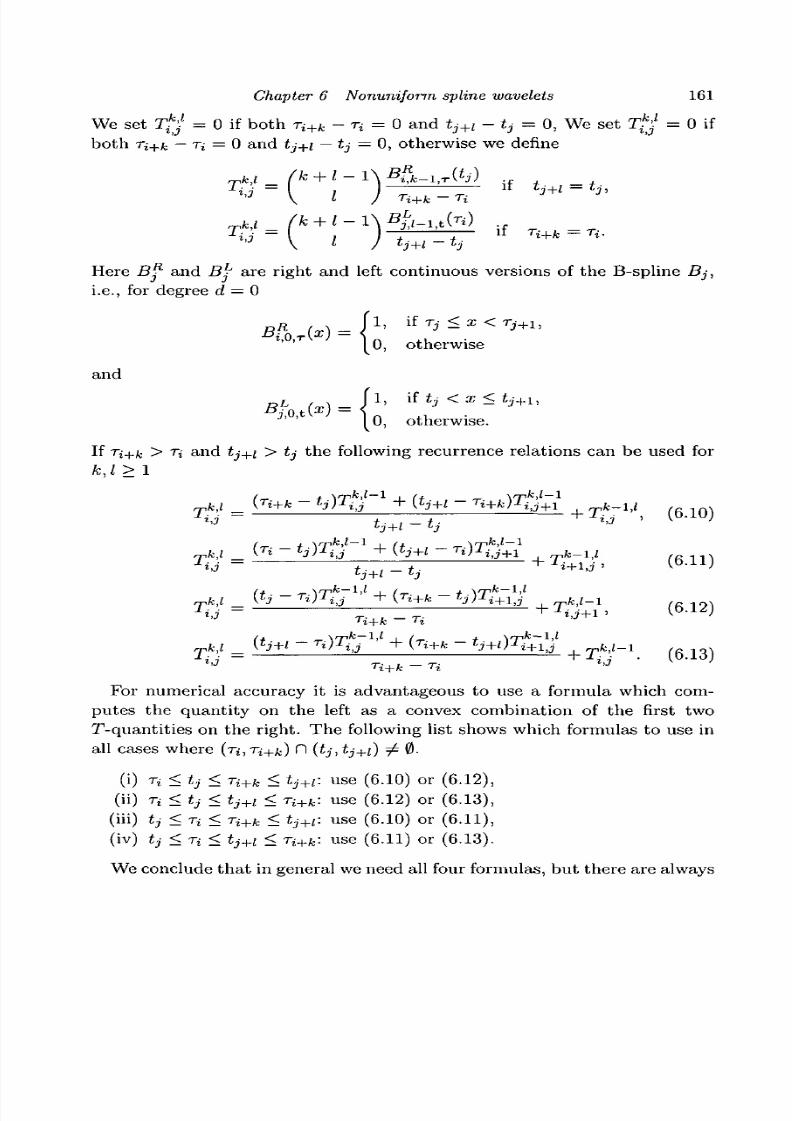
8/3/2019 Multivariate Approximation
http://slidepdf.com/reader/full/multivariate-approximation 171/296
Chapter 6 Nonuniform spline wavelets 161
We set ifj = 0 if both ri+k - n = 0 and tj+l - tj = 0, We set T*j = 0 if
b o t h Ti+k — T~i = 0 and tj+i — tj = 0, otherwise we define
l f
-T i
*-— if
Here Bj* and B^ are right and left continuous versions of the B-spline Bj,
i.e., for degree d = 0
D, otherwise
and
), otherwise.
If Ti+k > Ti and tj+i > tj the following recurrence relations can be used fork,l > 1
j + ( '+1 ~r)
rj
k,l _ (*j ~T
' ) '7i,j '
Ti . = — — I +
Ti. • (
6-
13)
For numerical accuracy it is advantageous to use a formula which com-
putes the quantity on the left as a convex combination of the first two
T-quantities on the right. The following list shows which formulas to use in
all cases where {Ti,T i+k) ("I (tj,tj+i) / 0.
(i) Ti < tj < T i+ k < tj+r. use (6.10) or (6.12),
(ii) n < tj < tj+i < T i+k: use (6.12) or (6.13),
(iii) tj <n< T i+ k < tj+l: use (6.10) or (6.11),
(iv) tj <n< tj+i < T l+k: use (6.11) or (6.13).
We conclude that in general we need all four formulas, b ut there are always

8/3/2019 Multivariate Approximation
http://slidepdf.com/reader/full/multivariate-approximation 172/296
162 T. Lyche, K. M0rken and E. Quak
at least two stable choices. If r = t and d = e one needs only two of the
formulas, see de Boor et al. (1976) for a numerically stable implementation.
6.3 Spline wavelets
An important and natura l example of a multiresolution analysis on an inter-
val is provided by spline spaces. We need a collection of knot vectors (tJ)^2.0
such that t3"
1is a subsequence of V for j > 1, since this ensures th at Sd t J- i
is a subspace of Sdtj. Each space has a Riesz-basis of B-splines, and knot
insertion takes us from one space to the next. Consider two nested splinespaces SdT and Sd> t with general knot vectors such that r is a subsequence
of t. We assume that the dimension of Sd<T is n with n > d + 1, and that
the dimension of S^t is n + m s o t can be thought of as obtained from r by
inserting m new knots s = (si^-^. For simplicity we assume that
Tl = Td+l, Tn+l = Tn+d+l, a n d Td+l < S\ < S2 < • • • < Sm < T n + 1 ,
the general setting is discussed in Lyche and M0rken (1992). For notational
convenience we rename the two sets of B-splines to
<t>j = BjidiT, for j = l,...,n,
7 i = Bid}t, for i = 1 , . . . ,n + m.
We also set
Vo = SdtT and V\ = <Sd]tl
and denote the orthogonal complement of Vo in V\ by W.
In Lyche and M0rken (1992) it was shown how to construct a minimallysupported basis for W. Here we give an alternative presentation of this con-
struction that clarifies some details. From this new approach it also follows
quite easily that the constructed basis is the only minimally supported basis
for W.
The basic idea underlying the construction is simple. Any function in W
must be a linear combination of B-splines in V\. Since we want the support
of a typical basis function ip to be minimal, we want a linear combination
of as few consecutive B-splines in V\ as possible, say q altogether. Theconstraint is that ip must be orthogonal to all the s coarse B-splines whose
supports intersect the support of ip . Intuitively, the support of tp should be
minimal when the number of parameters is one greater than the number of
conditions, i.e., when q = s + 1, and this turns out to be the case. An extra
bonus is that in this case it is easy to write down an explicit formula for tp .
In this way the construction of minimally supported wavelets is reduced to

8/3/2019 Multivariate Approximation
http://slidepdf.com/reader/full/multivariate-approximation 173/296
Chapter 6 Nonuniform spline wavelets 163
the problem of f inding minimal intervals that can s u p p o r t a wavelet , and
we show that the to ta l number of such intervals agrees exactly with the
dimension of W.
6.3.1 Construction of minimally supported wavelets
A function ip in Vi with index suppor t [£ : r], where r > £, is a linear
combina t ion of th e r — £ + 1 fine B-splines -f = (7^, . . . , 7 r )r,
and is zero off the interval [te,tT+ d+i\- Let us assume tha t there are p =
p(£, r) > 0 old knots in the open interval (t(, tr+ j,+i), name l y Tk+i, • • • , Vc+p,
for some k = k(£,r). Ther e are t hen p + d + 1 coarse B-splines 4> =
(<t>k-d:--- ,^fc+p)T, whose supports intersect the interval (t(,tT+ ci+\)- Due
to the local supports of B-splines, the spline if) is or thogonal to VQ if an d
only if
(<j>i, ip) = 0, for i = k - d, ... , k + p,
or in t e r m s of t he Gr am ma t r i x
As the orthogonal i ty condi t ions are homogeneous , a non-trivial solution is
guaranteed to exist if t he number of pa r ame t e r s is str ict ly larger than the
number of condi t ions imposed, namely r — £ + 1 > p(£,r) + d + 1. In the
hope of obta in ing a wavelet ip with smal les t poss ible support we want this
inequali ty to be satisfied with r — £ as smal l as possible . This mot ivates the
following definition.
D e f i n i t i o n 6 . 3 . 1 The index interval [£ : r] is said to be minimal if
r-£>p(£,r) + d (6.14)
and there is no t rue subinterval [u : v] with this proper ty, i.e., if £ < u <
v < r and v — u > p(u, v) + d, then u = £ and v = r.
A minimal interval always exists for given r and t , as the condit ion (6.14)
is certainly satisfied for the index interval [1 : n + m]; a smal les t subinterval
for which (6.14) is t rue must therefore be m inim al. Also, since a mi n i ma l

8/3/2019 Multivariate Approximation
http://slidepdf.com/reader/full/multivariate-approximation 174/296
164 T. Lyche, K. M0rken and E. Quak
interval cannot contain other minimal intervals than itself, we observe that
if [£ \ : n ] and [£2 '• ^2] are two dist inct minimal intervals then
r i ) > 0 . (6.15)
L e m m a 6 . 3 . 2 For a minimal interval [£ : r] we have
so that for minimal intervals the numb er of parameters is exactly one larger
than the number of orthogonality conditions imposed.
Proof Suppose the contrary is t rue, i .e . , that [£: r] i s minimal , but r — £ >
p(£, r) + d + 1. We dist inguish between two cases. First , i f tg+\ < T^+I, we
havep(£+l,r) = p{£,r). But then r - ( £ + 1 ) > p(£+l,r) + d, contradictingthe minimal i ty of [£ : r\.
If, however, t(+i = T ^ + I a nd T^+I is a knot of multiplici ty s > 1 in
the knot sequence r , then we have p(£ + l , r ) = p(£,r) — s, and therefore
r — (£ + 1) > p(£ + 1, r) + d + s, again contradict ing the minimal i ty of [£ : r] .
D
Our aim is to construct a wavelet with as small a support as possible, so
let us clarify what exactly we mean by this.
D ef in i t i on 6 .3 .3 A nonzero func tion ip in Vi wi th support [u : v] is called
a B-wavelet if it is orthogonal to Sd,T, and if it has minimal support in the
sense that if g is another nonzero spline in W with suppor t [u : v], where
u < u < v < v, t hen u = u an d v = v.
Our next resul t shows that any minimal interval [£ : r] i s the suppor t
interval of a B-wavelet.
T h e o r e m 6 . 3 . 4 Let [£ : r ] be a minimal interval. Then the spline function
i>i.x) = E i = ^ w i 7 i ( ^ ) given by
ip(x) = det
({4>k-d,lt)
(<f>k+p, It)(6.16)
is a B-wavelet with index support [£ : r], its coefficients (u>i)Ti= e oscillate
strictly in sign, and tp itself has r — £ strong changes of sign in (t(, tr+d+i).
8/3/2019 Multivariate Approximation
http://slidepdf.com/reader/full/multivariate-approximation 175/296
Chapter 6 Nonu niform spline wavelets 165
Proof Expanding the determinant (6 .16) , we f ind that i){x) = Y^i=e.wili(
x) >
where Wi = (— l)T~ lVi, Vi = d e t G j , and
Q. — ( 4>k-d,- • • ,4>k+p
\ j 7 7 - - . 7 r
Consequently, the spline ip lies in V\ and its support is included in
\t: r\. Taking inner products of tp in (6.16) with any of the coarse B-splines
{4>k+j}P-^d yields a determinant with two identical rows and therefore es-
tablishes that tp is indeed orthogonal to VQ .
We next show that vg > 0. By a formula from Karlin (1968), p. 17, wehave
v t = /detf/1'
Jn \ < P k - d , •••, <Pk+v
where Cl denotes the set
^ = {(2/1.- •• ,Vr-e) : « < 2/1 < ••• < Vr-l < b}.
Theorem 6.2.1 immediately impl ies that V( > 0. Since th e B-sp lines are
continuous functions, i t is clear that V( will be positive if the integrand is
positive at some point in the interior of ft. But again, f rom Theorem 6.2.1,
we know that this happens i f
s u p p 0 4>k-d-i+i H s u p p 0 7 £ + i ^ 0, for i = 1, ...,r-e, (6.17)
where supp 0 / den otes the interior of the sup po rt of / . For i = r — £,we have
that supp0 cpk-d-i+i = (jk+ p,Tk+ v+d+i) and supp o 7 r = (tr,tr+d+1). Sincerk+p e (te,tr+d+i) but Tk+p+i > tr+d+i, we see that the condition in (6.17)
is satisfied in this case.
Suppose now that (6.17) does not hold for some integer i = j with 1 <
j < r — i, in other words
{Tk-d-i+j,Tk+ j) n (te+j,te+j+d+ i) = 0.
As condition (6.17) holds for i = r — £, this is only possible if rk+j < tg+j.But since r C t, this implies th at
Tk+i < t e + i , f o r i = j , j - l , . . . , l .
In particular, for i = 1 we then have
t(
8/3/2019 Multivariate Approximation
http://slidepdf.com/reader/full/multivariate-approximation 176/296
166 T. Lyche, K. M0rken and E. Quak
From Lem ma 6.3.2, we h&ver-£ = p{£, r)+d+l, but if Tk+\ has multiplicity
s > 1 in r , then p(£ + 1, r) = p(£, r) - s, and
r-(e+l)=p(e+l,r) + d + s>p(e+l,r) + d,
contradicting the minimality of [£ : r] . The conclusion is therefore that
vi > 0, and by an analogous proof we conclude tha t Vi > 0 for i = £+1,... , r.
It remains to show that tp is a B-wavelet. Note that vg > 0 implies that
the matrix G( is non-singular, so the only linear combination of 7M-I, . . . ,
7 r that satisfies all the orthogonality conditions is the trivial one. Similarly,
since the last coefficient vr is also positive, the submatrix G r is also non-singular, which shows that there cannot be a non-trivial combination of
7^ , . . . , 7 r_i in W. This shows that tp has minimal support.
That ip has r — I strong sign changes in (tg, ir+d+i) follows from Lemma 2
in Lyche and M0rken (1992). •
Note at this point th at as a consequence of the integral formulas of Section
6.2.3, the B-wavelet coefficients are in fact rational functions of the knots.
We cannot have more minimal intervals than new knots.
Lemma 6 .3 .5 The B-wavelets in W generated by different minimal inter-
vals are linearly independent and there are at most m of them.
Proof Suppose that we have s B-wavelets with index supports [£j : TJ] for
j = l,... ,s. Equation (6.15) implies that these B-wavelets may be ordered
so that £\ < £2 < • • • < £s, and from Lemma 6.2.2 we therefore know that
they are linearly independent. But since dim W = m it follows that s <m.•
As we shall see shortly, there are exactly m minimal intervals, so the
corresponding B-wavelets form a basis for W. The clue to this fact is an
explicit procedure for constructing minimal intervals, one for each new knot.
The equation r — £ — p(l, r) = d+ 1 implied by Lemma 6.3.2 for a minimal
interval can be rewritten as
r + d+l-£+l= p{£, r) + 2d + 3.
This relation can be interpreted as stating that, apart from the p(£, r) old
knots in (t(,tr+ (i+i) , there are 2d + 3 knots in the index interval [£ : r ] .
More precisely, there must be 2d + 3 — pt(t) — \t(r + d + 1) new knots Si
in (ti,tr+d+i). As the multiplicity of any given knot is at most d+ 1, there
has to be at least one such new knot.
8/3/2019 Multivariate Approximation
http://slidepdf.com/reader/full/multivariate-approximation 177/296
Chapter 6 Nonuniform spline wavelets 167
If Sj is a new knot and t~ t and t? are two knots wi th t~ t < Sj < tf we define
the integer functions \ij and Vj by
We see that if [£ : r] is a minimal interval and Sj is a new knot in (tg, tr+,i+i)
then the relation
pt(e) + fij(e) + Vj(r + d + 1) + \t(r + d+l)=2d + 2 (6.18)
must hold (the sum is 2d + 2 since Sj is not counted in (6 .18)) . How-
ever, equation (6.18) is not sufficient to ensure minimal i ty , but the following
proposit ion gives a "symmet r ic" cons t ruc t ion of a minimal interval .
P r o p o s i t i o n 6.3.6 Let Sj be a new knot, let I be the largest integer less
than j such that
d+l, (6.19)
and let r be the smallest integer greater than j such that
Vj(r + d+l) + Xt(r + d+l) = d+l. (6.20)
Then [£ : r] is a minimal interval.
Proof We first show that the construction is well-defined in that integers
t and r that satisfy (6.19) and (6.20) exist. That (6.19) can be satisfied
follows from three simple facts:
(i) H(l) + p t(l)>d+l;
(ii) if tq is the largest q such that tq < Sj, then Hj(q) + Pt(q) ^ d + 1;
(iii) if tp < Sj and p > 1 then fj,j(p -l) + p t(p-l) < MJ(P) + Pt(p) + 1, so
the left-hand side in (6.19) increases by at most one when £ is reduced
by one.
The first fact is immediate since pt(l) = d + 1, while the second follows
since no knots occur more than d + 1 times in t. The third fact is obvious
if ip_i = tp, while if tp_i < tp it follows from the three relations )ij(p — l) <
mt(tp)+fj,j(p), ptip— 1) = 1 and pt(p) = mt(tp). The existence of an integer
r that satisfies (6.20) follows similarly.
The selection of I and r ensures that r — £ = p(£, r) + 2d + 2, but not yet
that r — £ is minimal. So suppose that [£ : r] contains a minimal subinterval
8/3/2019 Multivariate Approximation
http://slidepdf.com/reader/full/multivariate-approximation 178/296
168 T. Lyche, K. M0rken and E. Quak
[£' : r']. Without loss we assume tha t £ < £' and r ' < r. If Sj 6 (t(i, tri+d+\)
we must have
since £ was chosen as the largest integer satisfying (6.19). Likewise we must
have
p t{£') + iij{£') + Vj(r' + d + 1) + A t (r ' + d + 1) < Id + 2
contradict ing (6.18) and thereby the minimal i ty of [£ ' : r'\.
Another possibi l i ty i s that Sj < tp. As we noted above, there must be a t
least one new knot, say Si, in (tei,tr>+d+i). Since Si also lies in (t(,tr+4+i)
we must have
and £ and r must be the largest and smallest integers that sat isfy these
equations respectively. But if £ < £' and r' < r we must have
so
Vi(r' + d + 1) + X t(r' + d + 1) < d + l + j - i ,
Pt{£') + m{£') + vi(r' + d + 1 ) + X t(r' + d+l)<2d
which again contradicts the minimal i ty of [£' : r'\. The final possibility is
t h a t Sj > t r '+ d+ i an d this can be tre ate d similarly. We therefore con clude
t h a t [£ : ?•] is m in im al . •
By applying the const ruct ion in Proposi t ion 6.3.6 to a l l m new knots we
obta in m minimal intervals, and each of these gives rise to a B-wavelet as
s ta ted in Theorem 6.3.4.
T h e o r e m 6 . 3 . 7 Let [£j : rj] be the m minimal intervals obtained by app ly-
ing the construction in Proposition 6.3.6 to each of the m new knots (SJ)1^,
with Si < • • • < sm, and let ipj denote the B-wavelet associated with [£ j : rj]
for j = 1, . . . , m. Then £\ < • • • < £m, r\ < • • • < rm, the m associated
B-wavelets {i/»j}''L1 are the only B-wavelets in W (apart from scaling), and
these B-wavelets form a basis for this space.
8/3/2019 Multivariate Approximation
http://slidepdf.com/reader/full/multivariate-approximation 179/296
Chapter 6 Nonuniform spline wavelets 169
Proof For fixed j with 2 < j < m we first show th a t lj-\ < tj and rj-\ < rj.
Since Sj-i < Sj it follows from the definition of the fe and rs that lj-\ < f;
and Tj-\ < rj. Suppose tha t £j-\ = lj = L By const ruct ion we then have
But then ^ j_ i (£) = Hj(£) which is impossible by the definition of the fis.
Similarly it follows that rj_i < rj .
I t remains to be shown that there are no other B-wavelets in W. Suppose
th a t i/> is a B-w avelet. Since th e B-w avelets {tpj}JL 1 form a basis for W we
have
h
for certain numbers (CJ)3?^ with Cjx and Cj2 nonzero. But since the left and
right ends of the index supports of {tpj}'jL1 are strictly increasing, we see
that the index support of tp is [£ jl : rj2]. Now, ip is a minimally supported
wavelet in W. This implies j \ = J2 and T> = cipj^ for some nonzero constantc. •
Lemma 11 in Lyche and M0rken (1992) gives the following alternative
representation of a B-wavelet .
L e m m a 6 . 3 . 8 Let [£ : r] be a minimal interval, let ip be the associated
B-wavelet, and let Tk+\, ••• , T"fc+P be the old knots in (tg,tr+ (i+i). Then
ip = D
d+ 1
9, where 6 is the spline of degree 2d + 1 given by
. . ,T k+p
and e is a nonzero constant.
This lemma shows that B-wavelets can, if desired, be computed from
smaller determinants than the one used in (6.16). Also since £+p = r — d—1
the p + 1 B-splines (i?i,2d+i,t)j=|
>
of degree Id + 1 only depend on the knots
Finally, we note that polynomial reproduction of degree d is obvious in
our spline setting since the spline spaces contain polynomials of degree dand the approximation method from the fine space to the coarse space is
orthogonal projection. In other words, polynomials of degree d can be pro-
jected from the fine space to the coarse space with zero error, i.e., the detail

8/3/2019 Multivariate Approximation
http://slidepdf.com/reader/full/multivariate-approximation 180/296
170 T. Lyche, K. M0rken and E. Quak
component in W will be zero. But this in turn means that all of W is orthog-
onal to polynomials of degree d, and in particular we have (ip,xl) = 0 for
i = 0, . . . , d.
6.4 Algorithms for decomposition and reconstruction
To implement the complete wavelet transform, we must first decide how to
choose the nested sequence of spaces {V/jj. If we are given a spline / in
a fine space V^, this means that we must determine which of the interior
knots from V/v to keep in VJV-I , then which knots from V}v-i to keep inVV-2 and so on. We consider various approaches to selecting subspaces and
then discuss reconstruction and decomposition using the B-wavelets that we
constructed in Section 6.3, see also Chui and De Villiers (1998).
6-4-1 Choosing the subspaces
The simplest choice is to keep every other knot in analogy with classicalwavelets. An obvious generalization is to choose a fraction fi/v and keep /i
out of every v knots. The advantage of this approach is its simplicity.
An alterna tive is to use information abo ut / when deciding which kno ts
to pass on to V/v_i, as in the knot removal strategy in Lyche and M0rken
(1988). In this strategy, given a spline function and a tolerance, the aim
is to remove as many knots from the spline as possible, without letting
the error exceed the tolerance. The knots are first ranked according to their
significance in the representa tion of the spline. As many knots as possible arethen removed, in the order of increasing significance, takin g some uniformity
constraints into account. The knots of the resulting approximation are then
ranked again and removed according to the same criterion. This process is
continued until no more knots can be removed.
Knot removal is clearly closely related to compression via wavelet de-
composition, in that we compute in both cases successive approximations
in coarser and coarser spaces. The difference is th at in knot removal, the
detail (error) functions are not stored, although they are computed (andrepresented in the fine space) in order to check the magnitude of the error.
Using knot removal it is possible to ensure that the approximation in Vjy-i
will have certain desirable properties, for example tha t the approximation is
so good that the error (the wavelet component of /) may be neglected. On
the other hand, it may be argued that this mixes two stages of the wavelet
analysis: the decomposition and th e analysis. For efficiency, the choice of
8/3/2019 Multivariate Approximation
http://slidepdf.com/reader/full/multivariate-approximation 181/296
Chapter 6 Nonuniform spline wavelets 171
the spaces in the wavelet decomposition ought to be independent of / , but
the following analysis must of course involve (the decomposed version of) / .
In the ranking part of knot removal in Lyche and M0rken (1988) each knot
is given a weight indicating its significance. Since each new knot is associated
with a spline wavelet one could instead use the wavelet coefficient as a weight
for the corresponding knot. In particular, it is possible to use a wavelet
decomposition in a knot removal strategy. We simply carry out a wavelet
transform on some nested sequence of spaces, defined, say, by removing
every second knot. The wavelets which remain after the thresholding using
a certain tolerance then define the knots which are the candidates to keep.
6.4-2 Basis transformations
Our aim here is to sketch efficient algorithms for working with the spline
wavelets th at we constructed in Section 6.3. We use the same notation and
let Vo and V\ be coarse and fine spline spaces of dimension n and n + m,
respectively, spanned by B-splines of degree d that we organize into two
vectors <f> and 7. The complement space W of dimension m is spanned by
the m B-wavelets ip = (V'j)TLi-
Together the two bases <j> a nd V* form a basis for V\ so we have the
standard wavelet relation
(</>T,*/>
T)= 7
T (PQ) = 7rM (6.21)
and its inverse
The matrix P is the knot insertion matrix, while the matrix Q shows how
the B-wavelets are related to the fine B-splines. It can be obtained from the
explicit representation for B-wavelets in equation (6.16). When P and Q
are known, the matrices A and B are also given, as a decomposition of the
inverse of M.
Due to the relation (6.21), any function f\ € V\ has two different repre-
sentations with uniquely determined coefficient vectors, namely
h = 7TCi = /o + 9 = </>
TCo + •«/'
Tw.
The computation of the coarse spline coefficients Co and the wavelet coeffi-
cients w, when given the fine spline coefficients ci , is referred to as decom-
position, while the converse procedure is referred to as reconstruction.

8/3/2019 Multivariate Approximation
http://slidepdf.com/reader/full/multivariate-approximation 182/296
172 T. Lyche, K. M0rken and E. Quak
Recons t ruc t ion is accomplished via the reconst ruct ion re la t ion
whereas decomposi t ion is based on the inverse relat ion
(6.22)
(6.23)
Let us f irst see how we can perform reconstruction.
6-4-3 Reconstruction
Once the two matr ices P and Q are known, reconst ruct ion is s t ra ightforward
with the relat ion (6.22), and since in many cases both P and Q are banded
matr ices , this is also efficient.
The ma t r i x P can be computed efficiently by the Oslo algor i thm, see
Cohen et al. (1980), Lyche and M0rken (1986) . Our primary concern here
is therefore the efficient computation of Q . From the re la tion ipT
= JTQ
we see that the jth column of Q gives the B-spline coefficients of ipj relat iveto the fine B-splines. More specifically, the j t h B-wavelet ipj with suppor t
[E j : rj] is given as in (6.16) with £ = £j, r = rj and p = Pj = p(Ej,rj).
Note however that we are free to choose a different scaling of ipj. D ue to
the al ternating coefficients of ipj according to Theorem 6.3.4, we have the
following.
L e m m a 6 . 4 . 1 Let \£j : rj] be the index support of the jth B-wavelet ipj,
scaled such that the absolute values of its B-spline coefficients add to one-Let pj = p(dj,Tj) be the number of old knots in {t^,, t^.+^+i)• The nonzero
B-spline coefficients ( f t j ) ^ . of ipj are given by the solution of the linear
system
(<t>k+Pj,'
1
{4>k+Pj ,
- 1
Qr-Xj
\ Qrj )
=
/ON
0
W
(6.24)
. . . (-lp-h)
and constitute the nonzero part of column j of Q.
The l inear system (6.24) can be solved by straightforward Gaussian el im-
inat ion wi thout pivot ing s ince the matr ix obtained by deleting the last row
is tota l ly posit ive. Recall th at the compu t a t i on of the inner produc t en-
t r ies can be carried ou t as discussed in Sect ion 6.2.3. Determinat ion of Q

8/3/2019 Multivariate Approximation
http://slidepdf.com/reader/full/multivariate-approximation 183/296
Chapter 6 Nonuniform spline wavelets 173
is therefore straightforw ard once a scaling has been chosen. We will discuss
scaling in some more detai l in Section 6.4.5.
6.4-4 Decomposition
The algorithm for reconstruction is straightforward, but it is not so simple
to devise a good decomposition algorithm. A direct computation of the
inverse M "1, and thereby of the matrices A and B needed in (6.23), results
in full matrices with corresponding loss of efficiency. The entries of these
matrices typically decay away from the main diagonals, and so one might
suggest setting all matrix elements below a certain threshold to zero in orderto obtain banded matrices. However, practical experience shows that such
a truncation leads to significant round-off errors.
An alternative is to treat the equation
(P Q ) ( w ) = C l ( 6 - 2 5 )
as a linear system with (P Q) as the coefficient matrix of size n + m , with
the given coefficients Ci in Vi as the right-hand side, and with Co and w as
the unknowns. If Gaussian elimination is used to solve this linear system we
need to use some kind of reordering of equations and/or unknowns. This is
because the matrix (P Q) will typically have zero diagonal elements. One
possibility is to reorder the unknowns and interlace the columns of P and
Q to obtain a new (globally) banded coefficient matrix, allowing the use of
a special banded system solver. Exactly how to do this interlacing is not
clear, but it seems reasonable to place column i of Q in a position such that
its nonzero entries are distributed as evenly as possible above and below the
diagonal.
A third approach is based on the fact that, due to the orthogonality
of the decomposition / i = /o + 9, the functions /o and g are in fact the
least squares best approximations to /i from Vo and W, respectively, and
can therefore be computed using normal equations. The normal equations
can be derived quite simply. The wavelet function (the error) g = fi — fo
should be orthogonal to Vo, i.e., to each coarse B-spline. Since f\ = ' y r c i
and /o = <p co these conditions can be expressed as a system of n linear
equations in n unknowns,
(0,4>r)co = <</>, 7
T>ci. (6.26)
The other set of normal equations are derived from the conditions that the
approximation fo = fi — g should be orthogonal to W, or equivalently to

8/3/2019 Multivariate Approximation
http://slidepdf.com/reader/full/multivariate-approximation 184/296
174 T. Lyche, K. M0rken and E. Quak
all the B-wavelets in W. With g = ip w this leads to m linear equations in
th e in unknowns w,
(i/>, i\> )w = (xp,7 )ci. (6.27)
To solve the systems (6.26) and (6.27) the four matrices involved must be
computed. The two matrices {4>,4>T} and (</>, •yT), consisting of inner prod-
ucts of B-splines, can be computed directly, using one of the techniques
described in Section 6.2.3. The other two matrices are most conveniently
computed by making use of the refinement equation (6.21) and relating the
matrices to the matrix (7, j
T
) of inner products of fine B-splines,
{il>, V) = QT
< 7 , 7T
)Q, (</>,7T) = Q
T<7,7
r> -
For computational efficiency it is important to exploit the bandedness of all
the matrices involved.
6-4-5 Stability considerations
I t is c o m m o n to require from a wavelet const ruct ion that the combined setof basis functions (< p0, ip0, tp1,...) form a Riesz basis as in (6.3), since this
ensures tha t we have a basis for all of L2[a,b] and tha t computa t ions wi th
the combined basis can be performed without excessive loss of accuracy.
For spline wavelets there are several interpreta t ions of "Riesz basis". If
the nested spaces {V^}^l0 are spline spaces of degree d, genera ted by kno t
vectors ( t-7)^ = 0 , the required inequali t ies are
j=0
where K\ and K2 are two constants such that K^Ki is not overly large.
However, in the case of splines there is one added complication in that the
constants may depend on the knots. It is therefore possible that we have
a Riesz basis in the case where each new interior knot is inserted half way
between two old knots, but that there are certain knot configurations where
one or both of the constants become infinite. The ultimate form of stabilitywould of course be that the constants are completely independent of the
knots, as is the case for B-splines, see (6.4). To our knowledge, very little is
known about the stability of spline wavelets at present; in fact it is not even
known whether we have stability in the simplest nonuniform case where the
knot intervals are halved each time.
In spite of the lack of results on stability of the wavelet construction, the
8/3/2019 Multivariate Approximation
http://slidepdf.com/reader/full/multivariate-approximation 185/296
Chapter 6 Nonuniform spline wavelets 175
stabil i ty of the B-spline basis also has consequences for wavelet computa-
tions. Recall that for B-splines B x = (Bi,d)™_1 on a knot vector r we have
the s tabi l i ty es t imate
JD^IIclla^llB^cll^Hclb, (6.28)
where the scaled B-spline B^T is defined by
/ d + l \1 / 2
BBiAr =\Ti+d+l - ri
Since
B iAT . (6.29)
*- — T
this implies that the largest eigenvalue of the Gram matrix (B T , B T ) is 1,
while the smallest is D^2, so the condi t ion number of the Gram matr ix
is D\. In other words, if the B-splines are scaled as in (6.29), then the
corresponding G ram m atr ix is a lways wel l -condi t ioned, w hi le if the s ta nd ard
scal ing is used, the condi t ion number may be propor t ional to the ra t io
mhii(Ti+d+1 - n) '
This means that i f the wavelet decomposi t ions are computed by solving nor-
mal equations, the coefficient matrix of the system (6.26) is well-conditioned
if the B-splines are scaled as in (6.29).
When working with B-splines i t is convenient , however, to work with the
part i t ion of unity normalization and rather scale the coefficient matrices in
the l inear system s so th a t they becom e well-condit ioned. We introd uce a nn x n diagonal matr ix E T with diagonal e lements (ri+d+i ~ Ti)/(d + 1) for
i = 1 , . . . , n and a similar (n + m ) x (n + m) diagona l mat r ix Et . Ins tead
of (6.26) we can then solve the system
which by the above analysis has a condi t ion number bounded independent ly
of the knot vectors.
The knot insert ion matrix P can also be scaled so that i ts condit ion num-be r is bo un de d. As before, we let t = (ii)™^™ be a refined k no t vec tor w hich
con tains r as a subseq uenc e, an d we let P be the m atr ix tha t relates the
two bases as in (6.9). In Lyche and M0rken (1988) i t was shown that two
more inequali t ies can be f i t ted into (6.28),
^O^llclla < ||B^c||2 < | |Pc| |2 < ||c[|2. (6.30)

8/3/2019 Multivariate Approximation
http://slidepdf.com/reader/full/multivariate-approximation 186/296
176 T. Lyche, K. M0rken and E. Quak
Here P is the scaled version of P given by
p = E t1 / 2
P E ; 1 / 2 .
Prom the inequalities in (6.30) it follows that the condition number of P
(defined as the ratio between its largest and smallest singular values) is
bounded by Dd- This in turn means that some care should be observed
when computing with the matrix (</>, 7 r ) = P ( 7 , 7 r ) . The lack of stability
results for the matrix Q means that we have no guarantee that the system
(6.27) can be solved accurately.
One suggestion for decomposition is to solve (6.25). Even if we use th escaled version P of P, we cannot guarantee the stability of the system as
long as the stability of Q is not under control.
So far we have only discussed stability with respect to the L2-norm, but
since the B-spline basis, scaled correctly, is stable in any L p-space, see (6.4),
one might tr y to establish stability in other norms as well. Stability with
respect to the L°°-norm would be of particula r interest. Gram matrices
are naturally related to the L2-norm, so it is more difficult to prove that
the systems (6.26) and (6.27) are stable in L°°. For the system (6.25) itis known that P (without any further scaling) has bounded L°° condition
number, and it appears likely that properly scaled versions of Q should be
stable both in L°° and in I? .
6.5 Tensor products and triangulations
In this section we briefly consider the bivariate setting, namely tensor
product spline wavelets and (piecewise linear) spline wavelets on arbitrary
bounded triangulations.
6.5.1 Tensor product spline wavelets
The generalization to the tensor product setting is fairly straightforward,
bu t is included for the sake of completeness. Let V\ = VQ © W be one
decomposition of a spline space as previously described, with corresponding
matrices P, Q, M, etc. and
Vi = Vo © W
another decomposition, as above, with dimensions n, m, and n + m, bases
7 , <p, and tp , and matrices P, Q, M, etc.
Then we have the decomposition of the tensor product space as
Vi x 7 i = (Vo x Vo) © (Vo x W) © (W x V o) © (W x W),

8/3/2019 Multivariate Approximation
http://slidepdf.com/reader/full/multivariate-approximation 187/296
Chapter 6 Nonuniform spline wavelets 177
i .e. , three mutually orthogonal wavelet spaces representing functions that
are (a) a coarse spline in the first and a wavelet in the second component ,
(b ) a wavelet in the first and a coarse spline in the second component , and
(c ) a wavelet in bo t h componen t s .
A function f\ in V\ x V\ can now be wri t ten using an (n + m) x (n + m)
coefficient matrix C1, namely
fi(x,y)=<y(x)TC1*y(y).
Similarly,
fo(x,y) = <j>(x)TC°<f>(y) € Vo x Vo
g^ l\x,y) = 4>(x)TT>^':4}(y) S Vb xW
g• '(x,y) = ip(x) D^ 4>(y) € W x VQ
g{3 )(x,y) = ij>(x)TD {3):$(y) € W x W.
The matrix multiplication formula for reconstruction then becomes
C1
= PfC0?
7+ D^^Q
7") + QCD^P
T+ D^
3'Q
T)
Direct decomposition means first solving n + m linear systems of size n + m
with M = (P Q) as coefficient matrix and the right-hand sides given by
the columns of C1, as in
( P Q ) R = C1
.
Splitting the resulting (n + m) x (n + m) matrix R into two parts of sizes
n x (n + rii) and m x (n + m), i.e.,
HZ)shows tha t the second phase consists of first solving n sys tems of size n + m
with coefficient matrix M = ( P Q ),
3\T
\rp
in order to dete rmine C° and D ^ \ and then solving m sys tems of size n+m,again with coefficient matrix M ,
to compute D( 2 )
and D( 3 )
.
8/3/2019 Multivariate Approximation
http://slidepdf.com/reader/full/multivariate-approximation 188/296
178 T. Lyche, K. M0rken and E. Quak
On the other hand, the normal equation approach amounts to solving the
matrix equationsFC°F = P ^ ^
HD^F =
for C°, D ^ , D<2\ and D<
3). Here F = (<j>,4>T), F = ( 0 , ^
T) , H = (V, V
T) ,
j<
and H = {ip, i\> ) are univariate Gram matrices. As in the direct decom-position, this is achieved by solving linear systems, in this case in the first
stage with the matrices F and H as coefficient matrices, and with the cor-
responding matrices F and H in the second.
6.5.2 Spline wavelets on triangulations
The bivariate non-tensor-product setting, i.e., the construction of compactly
supported piecewise polynomial spline wavelets on triangu lation s, poses con-siderable challenges. This is especially true if the given triangulation is
supposed to be bounded and arbitrary, and not an infinite uniform one,
for which wavelets based on box splines have been constructed, de Boor et
al. (1993).
Based on subdivision schemes it is possible to construct so-called surface
wavelets, see Lounsbery et al. (1997), even for surface triangulations of ar-
bitrary topology in 3D. These surface wavelets, however, possess in general
no closed-form polynomial spline representations.In the remainder of this section, we will consider only planar bounded tri-
angulations in the following sense. A triangle is the convex hull of three non-
collinear points [3:1,0:2, £3]m
K2, and this triangle has three edges [3:1,2:2],
[0:2,2:3] and [0:3,0:1]. Let To = { T i , . . . , TM} be a set of triangles and let
Q = (Jj=i ^i be their union. Then we say that To is a triangulation if
(i) the intersection T{C\Tj, i ^ j , is either empty or corresponds to a
common vertex or a common edge,
(ii) the number of boundary edges incident on a boundary vertex is two,
(iii) the region fi is simply connected.
Associated with To are the set £0 which consists of all edges of triangles
in To, and the set Vo which consists of all the vertices of %. By a boundary
vertex or boundary edge we mean a vertex or edge contained in the boundary
of 0. All other vertices and edges are interior.
8/3/2019 Multivariate Approximation
http://slidepdf.com/reader/full/multivariate-approximation 189/296
Chapter 6 Nonuniform spline wavelets 179
While it is possible to use very general refinement procedures in the uni-
variate setting we described earlier, it is necessary to restrict our attention to
uniform refinement of a triangulation in order to obtain the explicit results
outlined later on.
Given a triangulation TQ we consider its uniform refinement T\, the tri-
angulation formed by dividing each triangle [x\, £2,23] in % into four con-
gruent subtriangles. Specifically, if yi, j/2, 2/3a r e
the midpoints of the edges
[£2,0:3], [3:3,0:1], [2:1,2:2] respectively, then the subtriangles are
[2:1,2/2,2/3], [2/1,0:2,2/3], [2/1,2/2,2:3], [2/1,2/2,2/3]-
We clearly have Vo C Vi, and if we set V* = Vi \ Vo, we see that a vertex
in Vi is either a coarse vertex, namely an element of Vo, or a fine vertex, an
element of V*.
Contrary to the univariate setting, where the polynomial degree of the
splines was arbitrary, we are only aware of explicit results on triangular
spline wavelets of polynomial degree 1, i.e., piecewise linear functions.
Let Vj be the linear space of piecewise linear functions over Tj, in other
words, the set of functions which are linear over each triangle in 7} and
continuous over Q. It is then clear that
Vb C V i .As basis functions for the spaces Vb and V\, respectively, we choose the nodal
(or hat) functions, namely for each v € Vo, 4>v £ Vb such that 4>v{w) = Svw
for w £ Vo, and analogously, for each v € Vi, -fv € Vi such that 7«(w) = Svw
for w € Vi. The basis sets of nodal functions are then <j)=
{^tilugvan<
^
7 = {ryv}ve\>r Their cardinalities, and thus the dimensions of the spaces Vb
and Vi, are |Vo| and |Vi|, respectively.
Note that the support of 4> v is the union of all triangles which contain the
vertex v £ Vo, called the cell ofv, which we denote by
Cv-.= U T.
veT
We can define an inner product (•, •) on L2(f2) by
where a(T) is the area of triangle T. With respect to this (weighted) inner
product, the spaces Vj become Hilbert spaces, with corresponding (weighted)
8/3/2019 Multivariate Approximation
http://slidepdf.com/reader/full/multivariate-approximation 190/296
180 T. Lyche, K. M0rken and E. Quak
2-norm ||/ | | 2 = (f,/)1^2- This norm is equivalent to the unweighted L2-
norm . In principle, it is also possible to use the standard , nonweighted
inner product, and obtain similar results, but the use of the inner product
in (6.31) results in a considerable reduction of the computations necessary
to determine the wavelet coefficients, which is especially important for ap-
plications in computer graphics (see Lounsbery et al. (1997)).
Let W denote the relative orthogonal complement of the coarse space Vo
in the fine space V\ with respect to the inner product (6.31), so that
Vi = VQ® W.
The dimension of W is |£o| = |Vi| — |Vo|. Therefore, a basis of W is typically
described by associating one basis element with each edge in the triangula-
tion To, or equivalently, with each midpoint of such an edge.
We let the coarse vertices v, v* € Vo be the endpoints of the edge [v , v*] 6
<?o, which has the midpoint « 6 V , . Finding a wavelet basis {ipu}u^v , of W
thus amounts to first describing the construction of an element tp u € V\ that
actually lies in W, and then showing that the whole set of these elements
in W is linearly independen t. Additionally, the tota l collection should bestable, i.e., satisfy inequality (6.3).
The surface wavelet construction in Lounsbery et al. (1997), when spe-
cialized to th is planar piecewise linear setting, sta rts with a fine ha t function
7U. Letting Lo(7u) denote the orthogonal projection of yu onto Vo using the
inner product (6.31), the difference yu — £o(7u) is a wavelet in W. This
function, however, has global support on all of f2, while for computational
reasons it would be desirable to have a locally supported basis for W.
We are aware of only two (different and independently developed) ap-proaches for obtaining a basis for W with local support. Th e one in Steven-
son (1998) originates from the numerical treatment of PDEs and can be
generalized to higher dimensions, bu t produces piecewise linear spline wave-
lets, whose supports are somewhat larger than for the wavelets studied in
Floater and Quak (2000) and Floater et al. (2000). The latter construction
is based on an approach for computing directly the orthogonality conditions
that are imposed for minimally supported elements of the wavelet space.
More specifically, the two different strategies share the common approachthat for each coarse vertex v 6 Vo, some kind of auxiliary function in V\ is
defined whose support lies in the cell Cv, and which satisfies most, but not all
orthogonality conditions needed for an element in W. A linear combination
of auxiliary functions corresponding to several coarse vertices is then used
to produce an element in V\ satisfying all orthogonality conditions, i.e., a
true wavelet.

8/3/2019 Multivariate Approximation
http://slidepdf.com/reader/full/multivariate-approximation 191/296
8/3/2019 Multivariate Approximation
http://slidepdf.com/reader/full/multivariate-approximation 192/296
182 T. Lyche, K. M0rken and E. Quak
6.6 Discu ssion of som e exam ples
Perhaps th e simplest situation is the one where t is obtained from r byadding one knot. The corresponding wavelet space is one-dimensional and
the only B-wavelet is globally supported. The wavelet coefficient of a given
function / then gives an indication of the importance of the new knot for
the representation of /.
In recent years there has been considerable interest in so-called multi-
wavelets. Spline multiwavelets result from wavelet constructions on uniform
knot vectors where each knot has a fixed multiplicity r. If the knots are at
the integers, the complete B-spline basis is generated by r distinct B-splinesand their integer transla tes. This is clearly a special case of our construc-
tion. Th e classical wavelet theory generalizes nicely to multiwavelets, see
for example Strela (1996) and the references therein.
In some cases, for example for closed parametric curves, it is useful to deal
with splines which are periodic on some interval [a, b]. For n, d € N with
n > d + 2 let t = (ij)™^^"1"1 be a knot sequence with t^+i = a, tn+ a+i = b
and ti+n = ti + b — a for i = 1, 2 , . . . , 2d + 1. On this (b — (i)-periodic
knot sequence we can define periodic B-splines which form a basis for aspace of periodic splines. The dimension of this space is n. We refer to
Schumaker (1981) for further details . Spline wavelets can be constructed
for nested periodic spline spaces, see Lyche and Schumaker (2000) for the
quadratic, trigonometric spline case. In general the matrices P and Q will
be as in the non-periodic case except that we get a few corner elements due
to wraparound of some columns.
Th e stand ard adap tatio n of any kind of wavelet approach to an interval, as
mentioned already in the introduction, is to keep most of the interior scalingand wavelet functions, i.e., functions whose supports lie completely within
the interval. Special boundary scaling and wavelet functions are then intro-
duced using approaches depending on the specific type of multiresolution
analysis. For spline wavelets of degree d, this means that uniform dyadic
knots are used in the interior of the interval, with knots of multiplicity d + 1
at the interval endpoints, i.e., for nonnegative integers d, n the knot sequence
is
d+i
} | k < T -
This setting was first considered in Chui and Quak (1992). The cor-
responding decomposition and reconstruction algorithms were investigated
in Quak and Weyrich (1994a), their tensor-product versions in Quak and

8/3/2019 Multivariate Approximation
http://slidepdf.com/reader/full/multivariate-approximation 193/296
Chapter 6 Nonuniform spline wavelets 183
Weyrich (1994b), and a spline wavelet packet approach in Quak and Weyrich
(1997).
As a typical and very frequently used example, let us consider the cubic
case d = 3, for which we want to provide all numerical values needed to
implem ent the algorithms of Section 6.4. Consider specifically the knot
sequences r = 113,3a n
d its uniform refinement t = 113,4. The corresponding
spline spaces Vo and V\ are of course nested, have dimensions 11 and 19,
respectively, and contain all polynomials of degree 3. The corresponding
matrices P and Q thus have dimensions 19 x 11 and 19 x 8 and are given
below. These matrices contain the information that is necessary also for any
n > 4, as further refinement only leads to more interior columns, while the
number of boundary columns as well as their entries remain unchanged.
16P =
f16
8
0
0
0
0
0
0
0
0
0
0
0
0
0
0
0
0
I 0
0
8
12
3
0
0
0
0
0
0
0
0
0
0
0
0
0
0
0
0
0
4
11
8
2
0
0
0
0
0
0
0
0
0
0
0
0
0
0
0
0
2
8
12
8
2
0
0
0
0
0
0
0
0
0
0
0
0
0
0
0
0
2
8
12
8
2
0
0
0
0
0
0
0
0
0
0
0
0
0
0
0
0
2
8
12
8
2
0
0
0
0
0
0
0
0
0
0
0
0
0
0
0
0
2
8
12
8
2
0
0
0
0
0
0
0
0
0
0
0
0
0
0
0
0
2
8
12
8
2
0
0
0
0
0
0
0
0
0
0
0
0
0
0
0
0
2
8
11
4
0
0
0
0
0
0
0
0
0
0
0
0
0
0
0
0
0
3
12
8
0
0
0
0
0
0
0
0
0
0
0
0
0
0
0
0
0
0
8
If
Note that the entries of Q near the boundary differ somewhat from thosederived in Quak and Weyrich (1994a). There, the boundary spline wavelets
were constructed in order to preserve as many coefficients from the interior
elements as possible. Consequently, the bound ary spline wavelets in Quak
and Weyrich (1994a) are not B-wavelets, in the sense that their index sup-
ports are not minimal. Their actual support intervals, however, are the same
as for the B-wavelets.

8/3/2019 Multivariate Approximation
http://slidepdf.com/reader/full/multivariate-approximation 194/296
184 T. Lyche, K. M0rken and E. Quak
The matrix Q as given here offers also a nice illustration of the as yet un-
solved problem of how the various B-wavelets, i.e., the columns of Q, should
be scaled. Here, more or less arbitrarily and jus t to save some space, each
column has 1 and —124 as its first (or last) two nonzero entries. To achieve
the scaling as in Lemma 6.4.1, for example, the two interior columns need
to be multiplied by 1/80640, the first and last one by 27877/5025860410,
the second and next to last by 82900002/876051996025, and the third and
third to last by 1584/130442935.
Q =
1136914560
1655323200
27877
1321223960
27877
633094403
27877
229000092
27877
46819570
27877
-124
1
0
0
0
0
0
0
0
0
0
0
0
0
9450650880
77583612430
4145001
409599117799
16580004
36869700393
1381667
157389496903
8290002
32916268667
4145001
27809640281
16580004
-124
1
0
0
0
0
0
0
0
0
0
0
0
153545
396
6643465
3168
738445
88
29839177
1584
19335989
792
58651607
3168
521819
6 6 ~
442733
-124
1
0
0
0
0
0
0
0
0
0
0
1
-124
1677
-7904
18482
-24264
18482
-7904
1677
-124
1
0
0
0
0
0
0
0
0
0
0
1
-124
1677
-7904
18482
-24264
18482
-7904
1677
-124
1
0
0
0
0
0
0
0
0
0
0
1
- 1 2 4
442733
26 4
- 1 2 4
27809640281
16580004
32916268667
4145001
157389496903
8290002
36869700393
409599117799
16580004
77583612430
-124
1655323200
27877
1136914560
27877
In this special case, it is possible to determ ine a strategy for interlacing the
columns of P and Q to obtain a banded square matrix, allowing to imple-ment decomposition by solving the (permuted) system by means of a special
banded system solver. For each column of P and Q, respectively, the index
of the row which contains the element of largest absolute value is determined.
This index then provides the column number for the overall square matrix
where the original column is to be placed. For the given example matr i-
ces, the columns of P thus become columns 1,3 ,4,6 ,8,10 ,12 ,14 ,16 ,17 ,19
8/3/2019 Multivariate Approximation
http://slidepdf.com/reader/full/multivariate-approximation 195/296
Chapter 6 Nonuniform spline wavelets 185
of the permuted square matrix, while the columns of Q become the columns
2,5,7,9,11,13,15,18.
In order to implement decomposition via the linear system (6.26), we need
the Gram matrices of the B-splines. Note again that in this special case, also
these Gram matrices differ only in the number of interior columns, while the
blocks corresponding to the boundary elements need to be computed only
once and can be used for all refinement levels.
The 19 x 19 inner product matrix is given by 40320 (7,/y
T) =
1 720
441
93
6
0
0
0
0
0
0
0
0
0
0
0
0
0
0
0
441
1116
1575
2
174
3
2
0
0
0
0
0
0
0
0
0
0
0
0
0
0
93
15752
6
174
16471132
0
32
239
2
1132 24161191
239
2
1
0
0
0
0
0
0
0
0
0
0
0
0
0
0
0
1
120
119124161191
120
1
0
0
0
0
0
0
0
0
0
0
0
0
0
0
0
1
120
119124161191
120
1
0
0
0
0
0
0
0
0
0
0
0
0
0
0
0
1
120
119124161191
120
1
0
0
0
0
0
0
0
0
0
0
0
0
0
0
0
1
120
119124161191
120
1
0
0
0
0
0
0
0
0
0
0
0
0
0
0
0
1
120
119124161191
120
1
0
0
0
0
0
0
0
0
0
0
0
0
0
0
0
1
120
119124161191
120
1
0
0
0
0
0
0
0
0
0
0
0
0
0
0
0
1
120
119124161191
120
1
0
0
0
0
0
0
0
0
0
0
0
0
0
0
0
1
120
119124161191
120
1
0
0
0
0
0
0
0
0
0
0
0
0
0
0
0
1
120
119124161191
120
1
0
0
0
0
0
0
0
0
0
0
0
0
0
0
0
1
120
119124161191
120
1
0
0
0
0
0
0
0
0
0
0
0
0
0
0
0
1
120
119124161191
120
1
0
0
0
0
0
0
0
0
0
0
0
0
0
0
0
1
239
2
119124161132
239
2
3
0
11321647
174
6
1575
93
0
0
0
0
0
0
0
0
0
0
0
0
0
0
3
2
174
1575
2
0
0
0
0
0
0
0
0
0
0
0
0
0
0
0
6
93
1116 441
441 720
ReferencesAhlberg, J.H. and Nilson, E.N. (1965). Orthogonality properties of spline
functions. J. Math. Anal. AppL, 11, 321-337.
Boor, C. de (1976). Splines as linear combinations of B-splines. A survey. In
Approximation Theory, II, ed. G.G. Lorentz, C.K. Chui and L.L. Schumaker,
pp. 1-47. Academic Press, New York.
Boor, C. de, Hollig, K. and Riemenschneider, S. (1993). Box Splines.
Springer-Verlag, New York.

8/3/2019 Multivariate Approximation
http://slidepdf.com/reader/full/multivariate-approximation 196/296
186 T. Lyche, K. M0rken and E. Quak
Boor, C. de, Lyche, T. and Schumaker, L.L. (1976). On calculating with B-splinesII. Integration. In Num erische Methoden der Approximationstheorie Vol. 3,
ISNM 30, ed. L. Collatz, G. Meinardus and H. Werner, pp. 123-146.Birkhauser Verlag, Basel.
Buhmann, M. and Micchelli, C.A. (1992). Spline prewavelets for non-uniformknots. Numer. Math., 6 1 , 455-474.
Carnicer, J.M., Dahmen, W. and Peiia, J.M. (1996). Local decomposition ofrefinable spaces and wavelets. Appl. Comput. Harmonic Anal., 3, 127-153.
Chui, C. (1992). An Introduction to Wavelets. Academic Press, Boston.Chui, C.K. and Quak, E.G. (1992). Wavelets on a bounded interval. In Numerical
Methods in Approximation Theory, ISNM 105, ed. D. Braess, L.L.Schumaker, pp. 53-75. Birkhauser, Basel.
Chui, C.K. and De Villiers, J. (1998). Spline-wavelets with arbitrary knots on abounded interval: Orthogonal decomposition and computational algorithms.Comm. in Appl. Anal., 4, 457—486.
Cohen, A., Daubechies, I. and Vial, P. (1993). Wavelets on the interval and fastwavelet transforms. Appl. Comput. Harmonic Anal., 1, 54-81.
Cohen, E., Lyche, T.and Riesenfeld, R. (1980). Discrete B-splines and subdivisiontechniques in computer-aided geometric design and computer graphics.Comp. Graphics and Image Proc, 14, 87-111.
Dahmen, W., Kunoth, A. and Urban, K. (1999). Biorthogonal spline wavelets onthe interval—stability and moment conditions. Appl. Comput. Harmonic
Anal., 6, 132-196.Daubechies, I. (1992). Ten Lectures on Wavelets. CBMS Conf. Series in Appl.
M ath., Vol. 61, SIAM, Philadelphia.Daubechies, I., Guskov, I., Schroder, P. and Sweldens, W. (1999). Wavelets on
irregular point sets. Phil. Trans. R. Soc. Lon. A., 357, 2397-2413.Floater, M.S. and Quak, E.G. (1999). Piecewise linear prewavelets on arbitrary
triangulations. Numer. Math, 82, 221-252.Floater, M.S. and Quak, E.G. (2000). Linear independence and stability of
piecewise linear prewavelets on arbitrary triangulations. SIAM J. Numer.Anal., 38, 58-79.
Floater, M.S., Quak, E.G. and Reimers, M. (2000). Filter bank algorithms forpiecewise linear prewavelets on arbitrary triangulations. J. Comp. and Appl.Math., to appear.
Karlin, S. (1968). Total Positivity. Stanford University Press, Stanford.Lounsbery, M., DeRose, T.D. and Warren, J. (1997). Multiresolution analysis for
surfaces of arbitrary topological type. ACM Trans. Graphics, 16, 34-73.Lyche, T. and M0rken, K. (1986). Making the Oslo algorithm more efficient.
SIAM J. Numer. Anal., 23 , 663-675.Lyche, T. and Morken, K. (1988). A data reduction strategy for splines. IMA J.
Numer. Anal., 8, 185-208.
Lyche, T. and M0rken, K. (1992). Spline-wavelets of minimal support. InNumerical Methods in Approximation Theory, ISNM 105, ed. D. Braess, L.L.Schumaker, pp. 177-194. Birkhauser, Basel.
Lyche, T. and Schumaker, L.L. (1994). L-spline wavelets. In Wavelets: Theory,Algorithms, and Applications, ed. C. Chui, L. Montefusco, and L. Puccio, pp.197-212. Academic Press, New York.
Lyche, T. and Schumaker, L.L. (2000). A multiresolution tensor spline method forfitting functions on the sphere. SIAM J. Scient. Comp., to appear.
8/3/2019 Multivariate Approximation
http://slidepdf.com/reader/full/multivariate-approximation 197/296
Chapter 6 Nonuniform spline wavelets 187
Meyer, Y. (1991). Ondelettes sur l'interval. Rev. Mat. Iberoamericana , 7, 115-133.M0rken, K. (1991). Some identities for products and degree raising of splines.
Constr. Approx., 7, 195-208.Phillips, J.L. and Hanson, R.J. (1974). Gauss quadrature rules with B-spline
weight functions. Math. Comp., 28 , 666.Quak, E.G. and Weyrich, N. (1994a). Decomposition and reconstruction
algorithms for spline wavelets on a bounded interval. Appl. Comput.Harmonic Anal., 1, 217-231.
Quak, E.G. and Weyrich, N. (1994b). Decomposition and reconstructionalgorithms for bivariate spline wavelets on the unit square. In Wavelets,Images, and Surface Fitting, ed. P.J. Laurent, A. Le Mehaute, andL.L. Schumaker, pp. 419-428. A.K. Peters, Boston.
Quak, E.G. and Weyrich, N. (1997). Algorithms for spline wavelet packets on aninterval. BIT, 37, 76-95.
Schumaker, L.L. (1981). Spline Functions: Basic Theory. Wiley-Interscience, NewYork.
Stevenson, R. (1998). Piecewise linear (pre-)wavelets on non-uniform meshes. InMultiyrid Methods V, ed. W. Hackbusch and G. Wittum, pp. 306-319.Springer, Berlin.
Strela, V. (1996). Multiwavelets: Theory and Applications. Ph.D. thesis, MIT.Sweldens, W. and Schroder, P. (1996). Building your own wavelets at home. In
Wavelets in Computer Graphics, ACM SIGGRAPH Course Notes.

8/3/2019 Multivariate Approximation
http://slidepdf.com/reader/full/multivariate-approximation 198/296
Applied and computational aspects of nonlinearwavelet approximation
A. COHEN
Abstract
Nonlinear approxim ation has recently found com putational applications such
as data compression, statistical estimation and adaptive schemes for par-
tial differential and integral equations, especially through the development
of wavelet-based methods. The goal of this chapter is to provide a short
survey of nonlinear wavelet approximation from the perspective of these
applications, as well as to highlight some remaining open questions.
7.1 Introduction
Numerous problems in approximation theory have in common the following
general setting: we are given a family of subsets (SN)N>O of a normed space
X, and for / € X, we consider the best approximation error
<rN(f):= inf \\f-g\\x. (7.1)geS
Typically, N represents the number of parameters needed to describe anelement in SN, and in most cases of interest, ONU) S o e s
t°z e r 0 as this
number tends to infinity.
For a given / we can then study the rate of approximation, i.e., the range
of r > 0 for which there exists a C > 0 such that
Mf) < CN~ r. (7.2)
Note that in order to study such an asymptotic behavior, we can use a
sequence of near best approximation, i.e., //v 6 SN such that
Wf-fN\\x<CaN(f),
with C > 1 independent of TV. Such a sequence always exists even when the
188
8/3/2019 Multivariate Approximation
http://slidepdf.com/reader/full/multivariate-approximation 199/296
Chap ter 7 Non linear wavelet approximation 189
infimum is not attained in (7.1), and clearly (7.2) is equivalent to the same
es t imate wi th | | / — /AT||A'm place of c^{f).
Linear approximation deals wi th the s i tuat ion when the SN are l inear
subspaces. Classical instances of l inear approximation families are the foll-
owing:
(1) polynomial approximat ion: SN:= TIN, the space of algebraic poly-
nomials of degree N;
(2) spline approximation with uniform knots: with some integer 0 < k <
m fixed, SN is the spline space on [0,1] consisting of Ck piecewise
polynomial functions of degree m on the intervals [j/N, (j + 1)/JV],j = 0 , . . . , i V - l ;
(3) linear approximation in a basis: given a basis (efc)fc>o in a Banach
space, SN '•= span(eo, • • •, e^r).
In al l these si tuations N is typically the dimension of SN, possibly up
to some m ul t iplicat ive con stant . In con tras t , nonlinear approximation ad-
dresses the s i tuat ion where the SN are not l inear spaces, but are st i l l typi-
cally characterized by O(N) para m eters . Ins tance s of nonl inear app roxim a-
tion families are the following:
(1) rational approximation: SN '•= {^ : p , ? e ^N}, the set of rational
functions of degree N;
(2) free-knot spline approximation: with some integer 0 < k < m fixed,
SN is the spline space on [0,1] with N free knots consisting of C k
piecewise polynomial functions of degree m on intervals [XJ, a^+i], for
all partitions 0 = XQ < x\ < • • • < x/v-i < %N = 1;
(3) ./V-term approxim ation in a basis: given a basis (efc)fc>o in a Banachspace, SN is the set of all possible combinations ^ZkeE
xkek with
# ( £ ) < N, where # ( £ ) is the cardinality of E.
Note that these examples are in some sense nonlinear generalizations of
the previous linear examples, since they include each of them as particular
subsets. Also note that in all of these examples (except for the splines with
uniform knots), we have the natural property SN C SJV+I, which expresses
the fact that the approximation is "refined" as N grows.On a theoretical level a basic problem both for linear and nonlinear ap-
proximation can be stated as follows:
Problem 1 Given a nonlinear family (SN)N>O, what are the analytic prop-
erties of a function f which ensure a prescribed rate <T/V(/) < CN~r
?
By "analytic properties", we typically have in mind smoothness, since we
8/3/2019 Multivariate Approximation
http://slidepdf.com/reader/full/multivariate-approximation 200/296
190 A. Cohen
know that in many contexts a prescribed rate r can be achieved provided
that / belongs to some smoothness class Xr C X. Ideally, one might hope
to identify the maximal class Xr such that the rate r is ensured, i.e., have a
sharp result of the type
feX r& aN(f) < CN~r.
Another basic problem, perhaps on a slightly more applied level, is the
effective construction of near best approximants.
P r o b l e m 2 Given a nonlinear family (SJV)JV>O> find a simple implementable
procedure f H-» fN g SN such that \\f - / J V | | X < CONU) for all N > 0.
In the case of linear approximation, this question is usually solved if we
can find a sequence of projectors PN '• X i-> SN such that ||PJV||A'->A' ^ K
with K independent of N (in this case, simply take /AT = -P/v/ and note that
11/ — /JV||X < (1 + K)<JN{f))- It is in general a more difficult problem in
the case of nonlinear methods. Since the 1960s, research in approximation
theory has evolved significantly toward nonlinear methods, in particular
solving the above two problems for various spaces SN-
More recently, nonlinear approximation has become a ttractive on a more
applied level, as a tool for understanding and analyzing the performance
of adaptive methods in signal and image processing, statistical estimation
and numerical simulation. This is in part due to the emergence of wavelet
bases for which simple N-term approximations (derived by thresholding the
coefficients) yield in some sense optimal adaptive approximations. In such
applications the problems that arise are typically the following.
Problem3
(data compression) How can we exploit the reduction of pa-rameters in the approximation of f by }N € SN from the perspective of
optimally encoding f by a small number of bits? This raises the question
of a proper quantization of these parameters, namely, a proper encoding of
these parameters by a finite number of bits.
Problem 4 (statistical estimation) Can we use nonlinear approximation as
a denoising scheme? Here we need to understand the interplay between the
approximation process and the presence of noise.
Problem 5 (numerical simulation) How can we compute a proper nonlinear
approximation of a function u which is not given to us as data but as the
solution of some problem F(u) = 0 ? This is in particular the goal of adaptive
refinement strategies in the numerical treatment of PDEs.
The goal of this chapter is to briefly survey the subject of nonlinear ap-
proximation, with particular focus on these last more applied questions,
8/3/2019 Multivariate Approximation
http://slidepdf.com/reader/full/multivariate-approximation 201/296
Chapter 7 Nonlinear wavelet approximation 191
and some emphasis on wavelet-based methods. We would like to point out
that these questions are also addressed in the survey paper DeVore (1997)
which contains a more substantial development of the theoretical aspects of
nonlinear approximation. We hope tha t this chapte r will be useful to the
non-expert who wants to ob tain a first general and intuitive view of the sub-
ject, motivated by its various applications, before going into a more detailed
study.
The chapter is organized as follows. To start, we discuss in Section 7.2 a
simple example, based on piecewise constant functions, which illustrates the
differences between linear and nonlinear approximation. In Section 7.3, we
address the important case of N-tevm wavelet approximation and thresh-
olding algorithm s. Applications to signal compression and estimation are
discussed in Section 7.4 and Section 7.5. Applications to adaptive numeri-
cal simulation are briefly described in Section 7.6. Finally, we conclude in
Section 7.7 with some remarks and open problems which naturally arise in
the multivariate setting.
7.2 A simple example
Let us consider the approximation of functions defined on the unit interval
I = [0,1] by piecewise constan t functions. More precisely, given a disjoint
partition of / into N subintervals IQ, ..., /jv_i,a n
d a function / in l}{I),
we shall approxim ate / on each Ik by its average aik{f) = |^fc|-1
Jj f{i)dt.
The resulting approximant can thus be written as
fc=l
where XA is the characteristic function of a set A, i.e., XA(X) = I if x £ A,
0 elsewhere.
If the Ik are fixed independently of /, then /jv is simply the orthogonal
projection of / onto the space of piecewise con stant functions on the par-
tition Ik , i.e., a linear approximation of / . A na tural choice is the uniform
partition Ik := [k/N, (k + 1)/N]. With such a choice, let us now considerthe error between / and /jv, for example in the L°° (uniform) metric. For
this, we shall assume th at / is in C(I), the space of continuous functions on
I. It is then clear that on each Ik we have
a/*( / ) l< supt,u£lk

8/3/2019 Multivariate Approximation
http://slidepdf.com/reader/full/multivariate-approximation 202/296
192 A. Cohen
We thus have the error estimate
11/ - /ivlloo < sup sup | / ( i ) - / ( u ) | . (7.3)k t.uSh
This can be converted into an estimate in terms of N, under some addi-
tional smoothness assumptions on /. In particular, if / has a bounded first
derivative, we have sup ti1i(E/jk \f(t) - f{u)\ < \h\\\f\\oo = N^Wf'W^, and
thus
11/ — /ATIIOO < JV^II/'lloo- (7-4)
Similarly, if / is in the Holder space Ca
for some a £ (0,1), we obtain an
estimate in O(N~a). By considering simple examples such as f(x) = xa
for
0 < a < 1, one can easily check that these rates are actually sharp.
If we now consider an adaptive partition where the Ik depend on the
function / itself, we enter the topic of nonlinear approximation. In order
to understand the potential gain in switching from uniform to adaptive
partitions, let us consider a function / such that / ' is integrable. Since we
have s u p t n e / j t \f(t) — f(u) \ < Jj \f'(t)\dt, we see that a natural choice of theIk can be made by equalizing the quantities J{ \f'(t)\dt = TV"1
Jo \f'(t)\dt,
so tha t, in view of the basic estimate (7.3), we obtain the error estimate
11/ - /yvlloo < iV-^l/'lll-
In comparison with the uniform/linear situation, we thus have obtained the
same rate as in (7.4) for a larger class of functions, since / ' is not assumed
to be bounded but only integrable. From a slightly different perspective, the
nonlinear approximation rate might be significantly better than the linear
rate for a fixed function / . For example, the function f(x) = xa, 0 < a < 1,
has the linear rate N~a
and the nonlinear rate ./V"1 since f'{x) = axa~
lis
in L\I).
The above construction of an adaptive partition based on balancing the
L1 norm of / ' is somewhat theoretical. In particular a suitable adaptive
approximation algorithm should also operate on functions which are not
in IV
1
'
1
.Let us
describetwo
natural algorithmsfor
buildingan
adaptivepartition.
The first one is sometimes known as adaptive splitting (see, e.g., DeVore
and Yu (1990)). Given a partition of [0,1], and any interval Ik of this parti-
tion, we split Ik into two subintervals of equal size if ||/ — ark{f)\\oo,ik > £,
otherwise we leave it as it was. Starting this procedure from the single
interval / = [0,1] and using a fixed tolerance e > 0 at each step, we

8/3/2019 Multivariate Approximation
http://slidepdf.com/reader/full/multivariate-approximation 203/296
Chapter 7 Nonlinear wavelet approximation 193
end up with an adaptive partition into dyadic intervals and a correspond-
ing piecewise constant approximation //v with N = N(e) pieces such that
11/ - /JVIIOO < e.
Another simple algorithm uses wavelet thresholding. Consider the decom-
position of / in the H aar basis
2 J - 1
/ = « / ( / ) + E E (/> ,*>^> (7-5)
j>0 fc=0
We recall that ip jtk = 2j/2
ip(2:
> • -k) with ip = X[0,i/2] - [1/2,1] •F o r e a c r i
j > 0, the sum Y2k=J}{f>''(Jj,k)i>j,k describes the fluctuation Pj+if — Pjf
where Pj is the projector onto the space Vj of piecewise constant functions
on the intervals Ijik = [2~^k,2~\k + 1)], k = 0 ,. . . ,2^ - 1. A natural
adaptive approximation can be obtained by retaining in (7.5) only the TV
largest contributions in the L°° metric, i.e., the indices (j, k) corresponding
to the N largest \\djtkipjtk\\oo = 2^2\djtk\, where dj^ '•— if,ipj,k)- Indeed,
since ip jtk has zero mean, we have | { / , V'j.fc)! < 2~J'/
2infcem ||/ - clloo,/^. so
th at fine scale contributions will be retained only in the regions of im por tantfluctuation, i.e., where they are needed to refine the approximation.
Both m ethods give rise to specific partitions and adaptive approximations
/AT. Ideally, one would hope that these partitions are optimal in the sense
that | | / — /AT II00 is up to a constant the best approxim ation error of / from
piecewise constants on ./V free intervals. This is not true for both algorithms,
but they are somehow close to this property in many senses. For example,
if / ' 6 IP for some p > 1, one can prove the rates O(N~q) for any q < 1.
Also note that both algorithms have natural generalizations to the case ofapproximation in the LP metric, by using ||/ — o-ih(f)\\p,ik > £ as a splitting
criterion or keeping the N largest \\dj^i,k\\p = 2J'1/
'2~
1/'p'|c(jifc|-
In this chapter we focus on the wavelet approach for the following rea-
son. In this approach the nonlinearity is reduced to a very simple operation
(thresholding according to the size of the coefficients), resulting in simple
and efficient algorithms for dealing with many applications, as well as a
relatively simple analysis of these applications.
7 .3 W avele t s and th resh o ld in g
Wavelet bases offer a simple and powerful setting for building nonlinear ap-
proximations of functions. Simple because a near-optimal approximation
is often achieved by a straightforward thresholding procedure; powerful be-

8/3/2019 Multivariate Approximation
http://slidepdf.com/reader/full/multivariate-approximation 204/296
194 A. Cohen
cause it is in some sense optimal for a large variety of smoothness classes
modeling the function to be approximated.
We first recall some general notations and features for these bases (seeDaubechies (1992) and Cohen (1999) for more deta ils). They are usually
associated with multiresolution approximation spaces (Vj)j>o such that Vj C
Vj+i and Vj is generated by a local basis {<fix)x&rj, where Tj is a set of indices
typically associated to a spatial discretization of mesh size hj ~ 2~-7. By
local we mean that the supports are controlled by
diam(supp(<pA)) < CT3
if A € Tj and are "almost disjoint" in the sense that
# ( {/i s r,- s.t. SUPP(I^A) n supp(<^u) / 0}) < c
\ ')
with C independent of A and j . A complement space Wj of Vj into Vj+i
is generated by a similar local basis (ipx)xeVp Vj = Fj+i \ Tj. The full
multiscale wavelet basis (V>A)A€V> V = Uj>oVj allows one to expand an
arbitrary function / into / = S A E V ^ A ^ A I where V := Uj>oVj and with the
convention that we incorporate the functions ((px)xer0 m to the first "layer"(V'A)A 6V0-
In the standard constructions of wavelets on the Euclidean space M.d, the
scaling functions have the form tpx = <Pj,fc = 2Jfd
/2<£(2^ • — k), k 6 Z
d, and
similarly for the wavelets, so that Tj is natu rally viewed as the uniform mesh
2~JZ
d. In the case of a general domain Q £ Rd, special adaptations of the
basis functions are required near the boundary dfl, which are accounted for
in the general notations Tj and Vj.
Wavelets need not be orthonormal, but one often requires that they con-stitute a Riesz basis of L 2(ft), i.e., their finite linear combinations are dense
in L2 and for all sequences (dA)Aevw e n a v e
the norm equivalence
2/ , | « A | •
1Aev 2 Aev
In such a case, the coefficients d\ in th e expansion of / are obta ined by a n
inner produc t dx = (f,tjjx)> where the dual wavelet tpx is a n L 2- funct ion. In
the s tandard b ior thogonal cons t ruc t ions , the dua l wave le t sys tem (ipx)x^v
is also buil t from nested spaces Vj and has s imilar local support proper t ies
as the pr imal wavelets ^A . The pract ical advantage of such a set t ing is the
possibi l ity of "switching" betw een th e "s ta nda rd" (or "nod al") discret izat ion
of / € Vj in the basis (</'A)Aer:, and i t s "mul t iscale" representat ion in the
basis {4>x)\x\<j by means of fast O{N) decompos i t ion and recons t ruc t ion
8/3/2019 Multivariate Approximation
http://slidepdf.com/reader/full/multivariate-approximation 205/296
Chapter 7 Nonlinear wavelet approximation 195
algorithms, where N ~ 2dj
denotes the dimension of Vj in the case where fl
is bounded.
An im por tant feature is the possibility of characterizing the sm oothness of
a function / through the numerical properties of its wavelet coefficients or of
the error of (linear) approximation || / — Pjf\\, where Pjf := J2\x\<j(f> VOO^A
is a projector onto Vj. In particular, for functions of d variables, Sobolev
spaces are characterized by
WfWh ~ \\Pof\\l + J222SJ
y-pif\ti~ £ 2 2 S | A W ' (7.6)
j>0 AeV
and fractional Holder classes by
\\c- ~ IIPo/lloo + sup 2 ^ | | / - Pjf Woo ~ sup 2(s+d
MM\dx\. (7.7)j> o A v
Such norm equivalences are essentially valid under the restriction that the
wavelet ip \ itself has slightly more than Hs
or Cs smoothness. They reflect
the intuitive idea that the linear approximation error ||/ — Pjf\\p decays like
O(2~ sj) or O{N-Sld) provided that / has "s derivatives in Lp". In order to
give a precise general statem ent for any p, one needs to introduce the Besovspaces Bp q which measure smoothness of order s > 0 in I? according to
where u,m(f,t)p := su P |h |< t | |A™/||P = su P|f t |< t || ^ o ( T ) ( - ! ) * / ( - * f t ) | | p ,
is the mth order IP modulus of smoothness and m is any integer strictly
larger than s. Recall that we have Hs
~ B | 2 for all s > 0, Cs
~ 5J,iO O
andW
s<
p~ Bp
pfor all
non-integers > 0 and p ^ 2. For
such classes,the characterization by approximation error or wavelet coefficients takes the
following form which generalizes (7.6) and (7.7):
Let us now turn to nonlinear wavelet approximation. Denoting by
the set of all possible iV-term combinations of wavelets, we are interested
in the behavior of <TJV(/) as defined in (7.1) for some given error norm
X. We first consider the case X = L2
and assume for simplicity that
the ip \ constitute an orthonormal basis. In this case, it is a straightforward
8/3/2019 Multivariate Approximation
http://slidepdf.com/reader/full/multivariate-approximation 206/296
196 A. Cohen
computation that the best TV-term approximation of a function / is achieved
by its truncated expansion
IN •=
where EN(/) contains the indices corresponding to the N largest \d\\. The
approximation error is thus given by
/ _ \ V / _ \ 1/2
= E E
where (dn)n>o is defined as the decreasing rearrangement of {\d\\, A g V}
(i.e., dn-i is the nth largest \d\\).
Consider now the Besov spaces B^T where s > 0 and r are linked by
1/T = 1/2 + s/d. According to the norm equivalence (7.8) we note that
these spaces are simply characterized by
Thus if / € B^T, we find that the decreasing rearrangement (dn)n>o satisfies
n- l
n\dn\r<E \dk\
r<E I*I
T= E l
d>l
T^ C
II/HB?,T < oo,fc=O fc>0 AgV
and therefore
|dn| < Cn~^\\f\\BsT. (7.9)
It follows that the approximation error is bounded by
(7.10)
At this stage let us make some remarks.
As was previously noted, the rate N~
s
l
d
can be achieved by linear approx-imation for functions having s derivative in L
2, i.e., functions in H
s. Just
as in the simple example of Section 7.2, the gain in switching to nonlinear
approximation is that the class B*T is larger than Hs. In particular B%T
contains discontinuous functions for arbitrarily large values of s, while
functions in Hs
are necessarily continuous if s > d/2.
Note that 0 < r < 2 and is monotonically decreasing in s.

8/3/2019 Multivariate Approximation
http://slidepdf.com/reader/full/multivariate-approximation 207/296
Chapter 7 Nonlinear wavelet approximation 197
The ra te (7.10) is implied by / e B^T. On the other hand it is easy
to check that (7.10) is equivalent to the property (7.9), which in itself is
equivalent to the property that the sequence (d\)\ev is in the weak space
F i p
• #({A : \d x\ < e}) < Ce~T}.
This shows th at the property / € B% T is almost equivalent to the rate
(7.10). One can easily check that the exact characterization of B^.T is
given by the stronger property ^N> i{.NsldcrN(f))
TN~
l< oo.
• The space B^ T is critically embedded in I? in the sense th at the injection is
not com pact. This can be viewed as an instance of the Sobolev embedding
theorem, or directly checked in terms of the non-compact embedding of
£T
into £2
when r < 2. In particular, B^.T is not contained in any Sobolev
space Hs
for s > 0. Therefore no convergence rate can be expected for
the linear approximation of functions in B^.T.
The general theory of nonlinear wavelet approximation developed by De-
Vore and his collaborators extends these results to various error norms, for
which the analysis is far more difficult than for the I? norm. This theoryis fully detailed in DeVore (1997), and we would like to summarize it by
stressing three main types of results, the first two answering, respectively,
problems 1 and 2 as described in the introduction.
Approximation and smoothness spaces Given an error norm || • ||x
corresponding to some smoothness space in d dimensions, the space Y of
those functions such that O"AT(/) = di s tx (/ , 5V) < CN~s/d
has a typical
description in terms of another smoothness space. Typically, \i X represents
r orders of smoothness in IP , then Y will represent r+ s orders of smoothnessin U with 1/r = 1/p + s/d and its injection in X is not compact. This
generic result has a graphical interpre tation displayed in Figure 7.1 . In
this figure, a point (r, 1/p) represents function spaces with smoothness r
in Lv, and the point Y sits s levels of smoothness above X on the critical
embedding line of slope d emanating from X. Of course in order to obtain
rigorous results, one needs to specify in each case the exact meaning of "s
derivatives in Lp" and/or slightly modify the property <TJV(/) < CN~
s/d.
For example, if X = LP for some p € (l,oo), then / € B*<T = Y with
1/r = 1/p + s/d if and only if Eiv>i[A r V d f f iv ( / ) ] r- / v " 1 < °°- O n e a l s o
needs to assume that the wavelet basis has sufficient smoothness, since itshould be at least contained in Y.
Realization of a near-best approximation For various error metrics X,
a near best approxim ation of / in SN is achieved by /N '•= J2\eAN(f) d\ip\

8/3/2019 Multivariate Approximation
http://slidepdf.com/reader/full/multivariate-approximation 208/296
198 A. Cohen
where d\ := (/, ip\) are the wavelet coefficients of / and A J V ( / ) is the set of
indices corresponding to the N largest contributions H ^ ^ A H X - This fact is
rather easy to prove when X is a Besov space, by using (7.8). A much more
elaborate proof is needed to show that it is also true for spaces such as IP
and Wm
'p
for 1 < p < oo, and for the Hardy spaces Hp
when p < 1 (see
Temlyakov (1998)).
Connections with other types of nonlinear approximation In the
univariate setting, the smoothness spaces Y characterized by a certain rate
of nonlinear approximation in X are essentially the same if we replace N-
term combinations of wavelets by splines with N free knots or by rationalfunctions of degree TV. The similarity between wavelets and free-knot splines
is intuitive since both methods allow the same kind of adaptive refinement,
either by inserting knots or by adding wavelet components at finer scales.
The similarities between free-knot spline approximation and rational approx-
imation were elucidated on by Petrushev (1988). However, the equivalence
between wavelets and these other types of approximation is not valid in
the m ultivariate context (see Section 7.7). Also closely related to A^-term
approximations are adaptive splitting procedures, which are generalizationsof the splitting procedure proposed in Section 7.2 to higher order piece-
wise polynomial approx imation (see e.g. DeVore and Yu (1990) and DeVore
(1997)). In the case of the exam ple of Section 7.2, we remark th at the piece-
wise constant approximation resulting from th e adap tive splitting procedure
can always be viewed as an A^-term approximation in the Haar system, in
which the ac tive coefficients have a certa in tree structure: if A = (j, k) is used
in the approximation, then (j — 1, [fc/2]) is also used at the previous coarser
level. Therefore the performances of adaptive splitting approximations areessentially equivalent to those of Af-term approximations with the additional
tree structure restriction. These performances have been studied in Cohen
et al. (1999b) where it is shown that the tree structure restriction does not
affect the order N~sld
of Af-term approximation in X ~ (1/p, r) if the space
Y ~ (1/T, r + s) is replaced by Y ~ (1/f, r + s) with 1/f < 1/r = 1/p + s/d.
7.4 Data compression
There exist many interesting applications of wavelets to signal processing
and we refer to Mallat (1998) for a deta iled overview. In this section and
in the following one, we would like to discuss two applications which exploit
the fact that certain signals - in particular images - have a sparse repre-
senta tion in wavelet bases. Nonlinear approximation theory allows us to

8/3/2019 Multivariate Approximation
http://slidepdf.com/reader/full/multivariate-approximation 209/296
Chapter 7 Non linear wavelet approximation 199
sspi
s+t •
s •
ices
Embedding
in X
/
C
c
] 0 ( N "t / d
) Cf 0 ( N "t / d
)
Linear / Nonlinear
- X : measurem ent of the error
(s derivatives in L )
1 1
(Slope d)
No embedding
i n X
1/p l/q=l/p +t/d LP spaces
Fig. 7.1. Graphical interpretation of linear and nonlinear approximation
"quantify" the level of sparsi ty in term s of the decay of the error of TV-term
approximation.
Prom a mathematica l point of view, the TV-term approxim ation of a signal
/ can already be viewed as a "compression" algorithm since we are reducing
the number of degrees of freedom which represent / . However, practical
compression means tha t th e approximation of / is represented by a finite
number of bits. Wavelet-based compression algorithms are a particular case
of transform coding algorithms which have the following general structure:
• Transformation: the original signal / is transformed into its representa tion
d (in our case of interest, the wavelet coefficients d = (d\)) by an invertible
transform TZ.
• Quantization: the representation d is replaced by an approximation d
which can only take a finite number of values. This approxim ation can
be encoded with a finite number of bits.
• Reconstruction: from the encoded signal, one can reconstruct d and there-
fore an approximation / = Tt~ld of the original signal /.

8/3/2019 Multivariate Approximation
http://slidepdf.com/reader/full/multivariate-approximation 210/296
200 A. Cohen
Therefore, a key issue is the development of appro priate quan tization stra te-
gies for the wavelet representation and the analysis of the error produced
by quantizing the wavelet coefficients. Such strategies should in some sense
minimize the distortion ||/ — f\\x for a prescribed number of bits N and
error metric X.
Of course this program only makes sense if we refer to a certain
model of the signal. In a determin istic context, one considers the error
supy ey | | / — f\\x for a given class Y, while in a stochastic context, one
considers the error E(\\f — f\\x) where the expectation is taken over the re-
alizations / of a stochastic process. In the following we shall indicate some
results in the deterministic context.
We shall discuss here the simple case of scalar quantization which amounts
to quantizing independently the coefficients d\ into approximations d\ in
order to produce d. Similarly to the distinction between linear and non-
linear approximation, we can distinguish between two types of quantization
strategies.
• Non-adaptive quantization: the number of bits which are used to representd\ depends only on the index A. In practice they typically depend on the
scale level |A|. Fewer bits are allocated to the fine scale coefficients which
have smaller values than the coarse scale coefficients in an averaged sense.
• Adaptive quantization: the map d\ i—> d\ and the number of bits which are
used to represent d\ depends both on A and on the amplitude value \d\\.
In practice they typically only depend on \d\\. More bits are allocated to
the large coefficients which correspond to different indices from one signal
to another.
The second strategy is clearly more appropriate for exploiting the sparsity
of the wavelet representation, since a large number of bits will be used only
for a small num ber of numerically significant coefficients.
In order to analyze this idea more precisely, let us consider the following
specific strategy. For a fixed e > 0, we allocate no bits to the details for which
\d\\ < s by setting d\ = 0. This amounts to thresholding them. We allocate
j bits to a detail for which 2^~x
£ < \d\\ < 2%. If the 2J
possible values ofd\ are taken equally spaced within th e range (—2%, — 2
:>~
1e) U (2 J'~1e, 2%),
we ensure that for all A
\d\-dx\<e.
If we measure the error in X = L2, assuming the ip \ are a Riesz basis, we
8/3/2019 Multivariate Approximation
http://slidepdf.com/reader/full/multivariate-approximation 211/296
Chapter 7 Nonlinear wavelet approximation 201
f ind that
I l / - / H ! ~ £ l ^ - ^ | 2 ^ £ 2 # ( { A = \dx\>e})+ Yl MA|2- (7.11)ASV {A:|dA|<£}
Note that the second term on the right-hand side is simply the error of
nonlinear approximation obtained by thresholding at the level e, while the
first term corresponds to the effect of quantizing the significant coefficients.
Let us now assume that the class of signals Y has a sparse wavelet rep-
resentation in the sense that there exists r < 2 and C > 0 such that for all
/ € Y we have d = (dA)Aey G £T
W(V), with ||d||^ < C, i.e., for all / 6 Y
#({A : \d x{f)\>r,})<Cr,-r. (7.12)
We have seen in the previous section that this property is satisfied when
| | / | |s»T < C for all f eY with 1/T = 1/2 + s/d and that it is equivalent
to the nonlinear approximation property <TJV < CN~sld. Using (7.12), we
can estimate both terms in (7.11) as follows: for the quantization term, we
simply obtain
£2#({A : \dx\ > e}) < Ce2-T,
while for the thresholding term we have
Y, l^l2
^ £2
~2
'£ 2
# ( {A
= \dx\ > e2-i~1}) < Ce
2~
T. (7.13)
{A:|dA|<£} j > 0
Recall that 0 < r < 2, so that the bounds tend to zero with e. Therefore
we find that the compression error is estimated by Ce1 - T
/2. We can also
estimate the number of bits Nq which are used to quantize the d\ accordingto
Comparing A^ and the compression error estimate, we find the striking
result that
11/ - / | | 2 < CNW-W = CAT-s/d
,
with C a constant independent of / g Y, At first sight, it seems that we
obtain with only N bits the same rate as for nonlinear approximation which
requires ./V real coefficients.
However, a specific additional difficulty of adaptive quantization is that
we also need to encode the addresses A such that 2J - 1
e < |d^| < 2J£. The bit
cost Na of this addressing can be significantly close to A^ or even higher. If

8/3/2019 Multivariate Approximation
http://slidepdf.com/reader/full/multivariate-approximation 212/296
202 A. Cohen
the class of signals is modeled by (7.12), we actually find th at iVa is infinite
since the large coefficients could be located anywhere. In order to have A^ <
Ce~T as well, and thus obtain the desired estim ate | | / —/H2 < CN~ sld with
N = Nq + Na, it is necessary to make some minor additional assumptions
on Y which restrict the location of the large coefficients, and to develop a
suitable addressing strategy.
The most efficient wavelet-compression algorithms, such as the one devel-
oped in Shapiro (1993), typically apply addressing strategies based on tree
structures within the indices A. We also refer to Cohen et al. (1999b) where
it is proved that such a strategy allows us to recover optimal rate/distortion
bounds, i.e., optimal behaviors of the compression error with respect to the
number of bits N, for various deterministic classes Y modeling the signals.
In practice such results can only be observed for a certain range of N,
since the original signal itself is most often given by a finite number of bits
No, e.g., a digital image. Therefore modeling the signal by a function class
and deriving rate/distortion bounds from this model is usually relevant only
for a low bit rate N « NQ, i.e., high compression ratio. One should then of
course address the questions of "what are the natural deterministic classeswhich model real signals" and "what can one say about the sparsity of
wavelet representations for these classes". An interesting example is given
by real images which are often modeled by the space BV of functions with
bounded variation. This function space represents functions which have one
order of smoothness in L 1in the sense tha t b oth components of their g radient
are finite measures. This includes in particular functions of the type Xn for
domains ft with boundaries of finite length. In Cohen et al. (1999c) it is
proved thatthe
wavelet coefficientsof a
function/ € BV are
sparsein the
sense th at they are in £*,. This allows us to expect a nonlinear approximation
error of the order of N~ ll2for images, and a similar rate for compression
provided that we can handle the addressing with a reasonable number of
bits. This last task turns out to be feasible, thanks to some additional
properties such as the L°°-boundedness of images.
7.5 Statistical estimation
In recent years, wavelet-based thresholding methods have been widely ap-
plied to a large range of problems in statistics such as density estimation,
white noise removal, nonparame tric regression, diffusion estim ation , (see the
pioneering work of Donoho et al. (1995)). In some sense the growing inter-
est in thresholding strategies represents a significant "switch" from linear to
nonlinear/adaptive methods.

8/3/2019 Multivariate Approximation
http://slidepdf.com/reader/full/multivariate-approximation 213/296
Chapter 7 Nonlinear wavelet approximation 203
Here we shall consider the simple white noise model. Tha t is, given a
function /(£) we observe on [0,1]
dg(t) = f(t)dt + edw(t),
where w(t) is a Brownian motion. In other words, we observe the function
/ with an add itive white Gaussian noise of variance e2. This model can
of course be generalized to higher dimensions. We are now interested in
constructing an estimator / from the data g. The most common measure
of the estimation error is in the m ean square sense. Assuming tha t / 6 I?
we are interested in the quantity E(\\f — /H^)- As with data compression,the design of an optimal estimation procedure in order to minimize the
mean square error is relative to a specific m odel of the signal / either by a
deterministic class Y or by a stochastic process.
Linear estimation methods define f by applying a linear operator to g. In
many practical situations this operator is translation invariant and amounts
to a filtering procedure, i.e., / = h * g. For example, in the case of a
second order stationary process, the Wiener filter gives an optimal solution
in terms of /i(w) := r(cj)/(r(o;) + e 2) where r(oj) is the power spectrum of /,i.e., the Fourier transform of r(u) := E(f(t)f(t + u)). Another frequently
used linear method is by projection on some finite-dimensional subspace
V, i.e., / = Pg = E n = i ( 5 i e n ) e n , where (e n )^ = 1 , (e n )^ = 1 are biorthogonal
bases of V and N := dim(V). In this case, using the fact that E(f) = Pf
(since the expectation of the noise and thus of its projection are zero), we
can estimate the error as follows:
£(11/ - /111) = E{\\Pf - /HI) + E{\\P(g - /)| |
2
)<E(\\Pf~fg)+CNe
2.
If P is an orthonormal projection, we can assume that e n = en is an or-
thonormal basis so that E(\\P(g - / ) | |2) = £ n £ ( | < / - <?,en)|
2) = £ n £
2,
and therefore the above constant C is equal to 1. Otherwise this constant
depends on the "angle" of the projection P. In the above estimation, the
first term E(\\Pf — /H2,) is the bias of the estimator. It reflects the approxi-
mation property of the spaceV
for the model, and typically decreases withthe dimension of V. Note that in the case of a deterministic class Y, it is
simply given by \\Pf — / | |2 - The second term CNe2 represents the variance
of the estimator which increases with the dimension of V. A good estimator
should find an optimal balance between these two terms.
Consider for instance the projection on the multiresolution space Vj, i.e.,
/ := 5Zm<j(<?,'0A)V'A! together with a deterministic model: th e functions /

8/3/2019 Multivariate Approximation
http://slidepdf.com/reader/full/multivariate-approximation 214/296
204 A. Cohen
satisfy
11/11*- < C, (7.14)
where Hs
is the Sobolev space of smoothness s. Then we can estimate
the bias by the linear approximation estimate C2~2s
i and the variance by
C2^e2
since the dimension of Vj adapted to [0,1] is of order V. Assuming
an a priori knowledge of the level s of the noise, we find that the scale level
balancing the bias and variance terms is j(e), where 2J(
e)(
1+2s) ~ E~
2. We
thus select as our estimator
With such a choice,
Let us make a few comments on this simple result.
• The convergence rate 4s/(14- 2s) of the estimator, as the noise level tends
to zero, improves with the smoothness of the model. It can be shown that
this is actually the optimal or minimax rate, in the sense that for any
estimation procedure, there always exist an / in the class (7.14) for which
we have E(\\f - fg) > c£4s
/(i+2»).
• One of the main limitations of the above estimator is that it depends not
only on the noise level (which in practice can often be evaluated), but also
on the modeling class itself since j(e) depends on s. A better estimator
should give an optimal rate for a large variety of function classes.
• The projection Pj^ is essentially equivalent to low pass filtering which
eliminates those frequencies larger than 2^e\ The practical drawbacks of
such denoising strategies are well known. While they remove the noise,
low-pass filters tend to blur the singularities of the signals, such as the
edge in an image. This problem is implicitly reflected in the fact that
signals with edges correspond to a value of s which cannot exceed 1/2
and therefore the convergence rate is at most O{s).
Let us now turn to nonlinear estimation methods based on wavelet thresh-
olding. The simplest thresholding estimator is denned by
where r(g;rj) = {A : \{g,'4>\)\ > r]}, i.e., discarding coefficients of the data
8/3/2019 Multivariate Approximation
http://slidepdf.com/reader/full/multivariate-approximation 215/296
Chapter 7 Nonlinear wavelet approximation 205
of size less than some r\ > 0. Let us remark that the wavelet coefficients of
the observed data can be expressed as
where the b\ are Gaussian variables. These variables have variance 1 if we
assume (which is always possible up to a renormalization) that H^AII!=
1-
In the case of an orthonormal basis the 6A are independent. Therefore the
observed coefficients appear as those of the real signal perturbed by an
additive noise of level e. It thus seems at first sight that a natural choice for
a threshold is to simply fix r\ := e, i.e., we can hope to remove most of thenoise, while preserving the most significant coefficients of the signal, which
is particularly appropriate if the wavelet decomposition of / is sparse.
In order to understand the rate that we could expect from such a proce-
dure, we shall again consider the class of signals described by (7.12). For the
moment, let us assume that we have an oracle which gives us the knowledge
of those A such that the wavelet coefficients of the real signal are larger than
e, so that we can build the modified estimator
7== E (9,ipx)Tpx- (7-16)
Agr(/;e)
In this case, / can be viewed as the projection Pg of g onto the space V(f, e)
spanned by {ipx:
A G T(f;e)}, so that we can estimate the error by a sum
of bias and variance terms according to
+ E(\\P(f-g)\\l)
For the bias term, we recognize the nonlinear approximation error which
is bounded by Ce2~
Taccording to (7.13). From the definition of the class
(7.12) we find that the variance term is also bounded by Ce2~
T. Thus, we
obtain for the oracle estimator the convergence rate £2~
T. In particular, if
we consider the model
ll/lk,r < c,
with 1/T = 1/2 + s, we obtain
£(H/~ " /111) < Ce2~
T= Ce
Let us again make a few comments.
8/3/2019 Multivariate Approximation
http://slidepdf.com/reader/full/multivariate-approximation 216/296

8/3/2019 Multivariate Approximation
http://slidepdf.com/reader/full/multivariate-approximation 217/296
Chapter 7 Nonlinear wavelet approximation 207
level, it is necessary to use adaptive discretizations which should typically
be more refined near the singularities.
In the finite element context, such discretizations are produced by mesh
refinement. Starting from an initial coarse triangulation, we allow further
subdivision of certain elements into finer triangles, and we define the dis-
cretization space according to this locally refined triangulation. This is of
course subject to certain rules, in particular that of preserving the confor-
mity of the discretization, e.g., when continuity of the finite elements is
required. The use of wavelet bases as an alternative to finite elements is still
in its infancy (some first surveys are Cohen (1999) and Dahmen (1997)),
and is strongly motivated by the possibility of producing simple adaptive
approximations. In the wavelet context, the more appropriate terminology
is space refinement. We directly produce an approximation space
VA := span{i/)A : A € A},
by selecting a set A such that VA is well-adapted to describe the solution of
our problem. If TV denotes the cardinality of the adapted finite element or
wavelet space, i.e., the number of degrees of freedom which are used in the
computations, we see that in both cases the numerical solution UN can be
viewed as an adaptive approximation of the solution u in a space EAT , which
depends on u.
A specific difficulty of adaptive numerical simulation is that the solution
u is unknown at the beginning, except for some rough a priori information
such as global smoothness. In particular the location and structure of the
singularities are often unknown, and therefore the design of an optimal dis-
cretization for a prescribed number of degrees of freedom is a much more
difficult task than simple compression of fully available data.
This difficulty has motivated the development of adaptive strategies based
on a posteriori analysis, i.e., using the currently computed numerical sol-
ution to update the discretization and derive a better adapted numerical
solution. In the finite element setting, such an analysis has been developed
since the 1970s (see Babuska and Reinboldt (1978) or Verfurth (1994)) in
terms of local error indicators which aim to measure the contribution of each
element to the error. The rule of thumb is then to refine the triangles which
exhibit the largest error indicators. More recently, similar error indicators
and refinement strategies have been also proposed in the wavelet context
(see Bertoluzza (1995) and Dahlke et al. (1997)).
Nonlinear approximation can be viewed as a benchmark for adaptive
strategies. If the solution u can be adaptively approximated in EAT with
an error O~N{U) in a certain norm X, we would ideally like that the adaptive

8/3/2019 Multivariate Approximation
http://slidepdf.com/reader/full/multivariate-approximation 218/296
208 A. Cohen
strategy produces an approximation UN € £/v such th at the error ||u — UN\\X
is of the same order as <r/v (U
) • In the case of wavelets this means that the
error produced by the adaptive scheme should be of the same order as the
error produced by keeping the TV largest coefficients of the exact solution.
In most instances, unfortunately, such a program cannot be achieved by
an adaptive strategy and a more reasonable goal is to obtain an optimal
asym pto tic ra te . That is, if <7jv(«) < CN~S
for some s > 0, then an op-
timal adaptive strategy should produce an error ||u — UN\\X < CN~S. An
additional im portant aspect is the co mputational cost of deriving u/v- A
computationally optimal strategy should produce UN in a number of opera-
tions which is proportional to TV. A typical instance of a computationally
optimal algorithm, for a fixed discretization, is the multigrid method for
linear elliptic PDEs.
It should be noted that very often the norm X in which one can hope for
an optimal error estimate is dictated by the problem at hand. For example,
in the case of an elliptic problem, this will typically be a Sobolev norm
equivalent to the energy norm (e.g., the H1 norm when solving the Laplace
equation).
Most existing wavelet adaptive schemes have in common the following
general structure. At some step n of the computation, a set A n is used to
represent the numerical solution UAU = ZaeA n ^AV'A- In the context of an
initial value problem of the type
d tu = E(u), u(x, 0) = uo(x),
the numerical solution at step n is typically an approximation to u at time
nAt where At is the time step of the resolution scheme. In the context of astationary problem of the type
F(«) = 0,
the numerical solution at step n is typically an approximation to u which
should converge to the exact solution as n tends to oo. Here E and F are
typically partial differential or integral operators, not necessarily linear. In
both cases, the derivation of (A n + i ,«A n + 1) from (Ara,MAn) usually contains
three basic steps.
• Refinement: a larger set A n+i with A n C A n+i is derived from an a
posteriori analysis of the computed coefficients d™, A £ A n.
• Computation: an interm ediate numerical solution un+i = YL\e\n j ^ A + 1 |0 A
is computed from un and the data of the problem.
• Coarsening: the smallest coefficients of un+i are thresholded, resulting in

8/3/2019 Multivariate Approximation
http://slidepdf.com/reader/full/multivariate-approximation 219/296

8/3/2019 Multivariate Approximation
http://slidepdf.com/reader/full/multivariate-approximation 220/296
210 A. Cohen
In the univariate case, i.e., when f2 is a simple interval, the number of nonzero
coefficients up to scale j is bounded by jK . Therefore, using N nonzerocoefficients at the coarsest levels gives an error estimate with exponential
decay
Mf)<\j>N/K
which is a spectacular improvement over the l inear rate. In the multivari-
ate case, the number of nonzero coefficients up to scale j i s bounded by
J2{=oK2id~1)l a n d t h u s b y K2(d-1^. Therefore, using N nonzero coeffi-cients at the coarsest levels gives an error est imate
<yN{})<
which is much less of an improvement. For example, in th e 2D case, we only
go from N~ llA to iV"1/
2by switching to nonlinear wavelet approximation.
This simple example illustrates the curse of dimensionality in the contextof nonlinear wavelet approximation. The main reason for the deg radation of
the approximation rate is the large number, K2^d~1^, of wavelets which are
needed to refine the boundary from level j to level j + 1. On the other hand,
if we view the boundary itself as the graph of a smooth function, it is clear
that approximating this graph with accuracy 2~3 should require significantly
fewer parameters than K2^d~1". This reveals the fundamental limitation of
wavelet bases. They fail to exploit the smoothness of the boundary and
therefore cannot captu re the simplicity of / in a small number of parame-ters. Another way of describing this limitation is by noting that nonlinear
wavelet approximation allows local refinement of the approximation, but
imposes some isotropy on this refinement process. In order to capture the
boundary with a small number of parameters, one would typically need to
refine more in the normal direction than in the tangential directions, i.e.,
apply anisotropic local refinement.
In this context, other approximation tools outperform wavelet bases. It
is easy to check that the use of piecewise constant functions on an adaptivepartition of N triangles in 2D will produce the rate <7AT(/) ~ O(N~
1),
precisely because one is allowed to use arbitrarily anisotropic triangles to
match th e boundary. In the case of rational functions we have an even
more spectacular result. If dQ, is C°°, then <TJV(/) < CrN~r
for any r > 0.
These remarks reveal that, in contrast to the ID case, free triangulations
or rational approximation outperform JV-term approximation, and could

8/3/2019 Multivariate Approximation
http://slidepdf.com/reader/full/multivariate-approximation 221/296
Chapter 7 Nonlinear wavelet approximation 211
be considered as a better tool in view of applications such as those which
were discussed thro ugh out th is chap ter. This is however not really true in
practice. In numerical simulation, rational functions are difficult to use and
free triangulations are often limited by shape constraints which restrict their
anisotropy. Neither method is being used in statistical estimation or da ta
compression, principally due to the absence of fast and robust algorithms
which would produce an op timal adaptive approximation in a similar m anner
to wavelet thresholding.
The development of new approximation and representation tools, which
could both capture anisotropic features, such as edges with a very small
number of parameters, and be implemented by fast and robust procedures,
is curren tly the object of active research. A significant breakthro ugh was
recently achieved by Donoho and Candes who developed representations into
ridgelet bases which possess the scale-space localization of wavelets together
with some directional selection (see e.g., Candes and Donoho (1999)). Such
bases allow us, for example, to recover with a simple thresholding procedure
the rate O(N~X) for a bivariate function which is smooth except along a
smooth curve of discontinuity.
References
Babuska, I. and Reinboldt, W.C. (1978). Error estimates for adaptive finiteelement computations. SIAM J. Numer. Anal., 15, 736-754.
Bertoluzza, S. (1995). A posteriori error estimates for the wavelet Galerkinmethod. Appl. Math. Lett, 8, 1-6.
Candes, E.J. and Donoho, D.L. (1999). Ridgelets: a key to higher-dimensionalintermittency? Phil. Trans. Roy. Soc. A, 357, 2459-2509.
Cohen, A. (1999). Wavelets in numerical analysis. In Handbook of Num ericalAnalysis, vol. VII, ed. P.G. Ciarlet and J.L. Lions. Elsevier, Amsterdam.
Cohen, A., Dahmen, W. and DeVore, R.A. (1999a). Adaptive wavelet methods forelliptic operator equations-convergence rate. Math. Comp., to appear.
Cohen, A., Dahmen, W., Daubechies, I. and DeVore, R.A. (1999b). Treeapproximation and optimal encoding. Preprint.
Cohen, A., DeVore, R.A., Petrushev, P. and Xu, H. (1999c). Nonlinearapproximation and the space BV(R2). Am er. Jour, of Math., 121, 587-628.
Dahlke, S., Dahmen, W., Hochmuth, R. and Schneider, R. (1997). Stablemultiscale bases and local error estimation for elliptic problems. Appl.
Numer. Math., 23, 21-47.Dahmen, W. (1997). Wavelet and multiscale methods for operator equations. Ada
Numerica, 6, 55-228.Daubechies, I. (1992). Ten Lectures on Wavelets. SIAM, Philadelphia.DeVore, R.A. (1997). Nonlinear approximation. Acta Numerica, 7, 51-150.DeVore R.A. and Yu, X.M. (1990). Degree of adaptive approximation. Math.
Comp., 55, 625-635.Donoho, D., Johnstone, I., Kerkyacharian, G, and Picard, D. (1995). Wavelet

8/3/2019 Multivariate Approximation
http://slidepdf.com/reader/full/multivariate-approximation 222/296
212 A. Cohen
shrinkage: asymptotia? (with discussion). Jour. Roy. Stat. Soc, 57, Series B,301-369.
Mallat, S. (1998). A Wavelet Tour of Signal Processing. Academic Press, NewYork.
Petrushev, P. (1988). Direct and converse theorems for spline and rationalapproximation and Besov spaces. In Function Spaces and Applications, ed .M. Cwikel, J. Peetre, Y. Sagher and H. Wallin, pp. 363-377. Lecture Notes inMath. 1302, Springer, Berlin.
Shapiro, J. (1993). Embedded image coding using zero trees of waveletcoefficients. IEEE Signal Processing, 4 1 , 3445-3462.
Temlyakov, V. (1998). The best m-term approximation and greedy algorithms.Adv. Comput. Math., 8, 249-265.
Verfiirth, R. (1994). A posteriori error estimation and adaptive mesh-refinementtechniques. J. Comp. Appl. Math., 50, 67-83.

8/3/2019 Multivariate Approximation
http://slidepdf.com/reader/full/multivariate-approximation 223/296
8
Subdivision, multiresolution and the construction of
scalable algorithms in computer graphicsP. SCHRODER
A b s t r a c t
Multiresolution representations are a critical tool in addressing complexity
issues (time and memory) for the large scenes typically found in computer
graphics applications. Many of these techniques are based on classical sub-
division techniques and their generalizations. In this chapter we review two
exemplary applications from this area, multiresolution surface editing and
semi-regular remeshing. The former is directed towards building algorithms
which are fast enough for interactive manipulation of complex surfaces ofarbitra ry topology. The latter is concerned with constructing smooth pa-
rameterizations for arbitrary topology surfaces as they typically arise from
3D scanning techniques. Remeshing such surfaces th en allows the use of
classical subdivision ideas. We focus in particular on the practical aspects
of making the well-understood mathematical machinery applicable and ac-
cessible to the very general settings encountered in practice.
8.1 Introduction
Many applications in computer graphics are dominated by the need to deal
efficiently with large datasets. This need arises from the goal of providing
the user with a responsive system (ideally) allowing interactive work, i.e.,
up da te ra tes of several frames per second. However, compelling or real-
istic datasets such as topographical maps or geometric models appearing
in entertainment and engineering tend to have large amounts of geometric
detail. One measure of the latter is the number of triangles or patches nec-
essary to provide a good approx imation of a given complex surface. Not
only must these datasets be displayed and transmitted rapidly, but in many
cases expensive numerical computations must be performed on this data.
Examples include surface denoising, fairing, compression, editing, optimiza-
213
8/3/2019 Multivariate Approximation
http://slidepdf.com/reader/full/multivariate-approximation 224/296
214 P. Schroder
tion, and finite element (FEM) computations. The target machines for such
computations are typically small workstations or home PCs with hardware
accelerated graphics adapters.
These needs provide the motivation to search for efficient representations
and algorithms which perform a variety of discrete and continuous compu-
tations. Some of the properties these representations and algorithms should
satisfy are:
• Scalability their time and space complexity should ideally be linear in
the inp ut size. Conversely algorithm s which require quad ratic space or
time are generally impractical as input sizes reach into the tens of thou-
sands or more primitives. Note that scalability can also mean the ability
to take advantage of large parallel computing resources. We will not dis-
cuss this issue further as our attention is directed towards small, widely
available computing platforms.
• Speed/Fidelity tradeoffs to provide the user with an interactive ex-
perience, algorithms that are capable of providing approximate answers
quickly, as well as more precise answers with additional time (and storage)
are preferred over algorithms that always provide highly accurate answers
after long computing times. For example, this requirement favors itera-
tive solvers over direct solvers, or wavelet methods which provide "control
knobs" for approximation quality versus computational time and storage.
• Intuitive control most applications in computer graphics involve a pos-
sibly naive user, thus the parameters exposed by the system must be
intuitive and should not require a deep understanding of the underly-
ing representa tions and a lgorithm s. For example, it is very difficult tomanipulate Fourier coefficients directly to achieve a desired effect, while
locally-supported functions such as B-splines provide an easy-to-grasp re-
lationship between cause and effect.
• Robustness the larger the input dataset the higher the probability that
all manner of "screw cases" will appear in a given da taset. Algorithms
must handle these in a robust fashion and ideally be insensitive to them.
• Uniformity a system which attempts to deal with many different rep-
resentations concurrently tends to be more complicated and fragile thanone which is based on a single, and very general representation.
One general concept which is now widely accepted as fundamental to the
construction of scalable algorithms is the idea of multiresolution. In the con-
text of computer graphics multiresolution comes in two fundamental flavors:
(a) constructions which are based on classical notions of multiresolution as

8/3/2019 Multivariate Approximation
http://slidepdf.com/reader/full/multivariate-approximation 225/296
Chapter 8 Scalable algorithms in computer graphics 215
Fig. 8.1. Multiresolution as it is defined through subdivision. Sta rting w ith a coars-est level mesh of arbitrary connectivity successive levels of a multiresolution rep-resentation are produced throu gh subdivision. (Original dat ase t courtesy HuguesHoppe.)
Fig. 8.2. M ultiresolution as it is defined thro ugh mesh simplification. Start ingwith a finest level mesh of arbitrary connectivity, successive levels of a multiresolu-tion represen tation are produced thro ugh simplification. (Original data set courtesyAvalon.)

8/3/2019 Multivariate Approximation
http://slidepdf.com/reader/full/multivariate-approximation 226/296
216 P. Schroder
they appear in wavelets and subdivision; and (b) constructions based on
mesh simplification (see Figures 8.1 and 8.2, respectively).
In the following we study two representative examples of these ideas. The
first concerns the construction of a multiresolution surface editor which al-
lows the manipulation of intricate, arbitrary topology surfaces at interactive
rates on low end platform s. It uses classical subdivision surfaces (Loop)
and extends them with the help of a Burt-Adelson type pyramid to a true
multiresolution setting, i.e., a setting with non-trivial details at finer resolu-
tions. The second application concerns the construction of smooth param-
eterizations for arbitrary connectivity meshes. Today, meshes that describe
detailed geometric objects are typically built throu gh 3D scanning. Before
these meshes become amenable to a number of numerical algorithms they
must be provided with a smooth param eterization. In particular th is is
the first step in transforming ("remeshing") them into a setting suitable for
subdivision-based multiresolution approaches.
The work discussed in the following was performed jointly with my (for-
mer) student Denis Zorin and long term collaborator Wim Sweldens. David
Dobkin and his student Aaron Lee participated in this work as well and Iam grateful to all of them.
8.2 Interactive multiresolution surface editing
Applications such as industrial and engineering design as well as special
effects and animation require creation and manipulation of intricate geo-
metric models of arbitrary global topology (genus, number of boundaries,
and connected com ponents). Like real world geometry, these models cancarry detail at many scales (see Figure 8.3). Such models are often created
with 3D range sensing devices such as laser scanners (see for example the
work of Curless and Levoy (1996)), and the resulting meshes can be com-
posed of as many as a million or more triangles. Manipu lating such fine
meshes is difficult, especially when they are to be edited or animated. Even
without accounting for any computation on the mesh itself, available ren-
dering resources alone may not be able to cope with the sheer size of the
data.A popular approach for addressing the complexity challenge posed by
such geometry is based on polygonal simplification (Heckbert and Garland
(1997)). This aims to produce a lower resolution polygonal model which
closely approximates the original geometry based on various error measures,
such as Hausdorff d istance or Sobolev norms. While these methods can
produce approximations using fewer polygons, ultimately a smooth rather

8/3/2019 Multivariate Approximation
http://slidepdf.com/reader/full/multivariate-approximation 227/296
Chapter 8 Scalable algorithms in computer graphics 217
Fig. 8.3. Before the Armadillo started working out he was flabby, complete witha double chin. Now he exercises regularly. The original is on the right (courtesyVenkat Krishnamurthy, Stanford University). The edited version on the left illus-trates large scale edits, such as his belly, and smaller scale edits such as his doublechin; all edits were performed at about 5 frames per second on an Indigo R10000Solid Impact.
than piecewise l inear representations is desired. For example, a set of spline
patches which approximates the or iginal geometry. Finding such approxima-
tions is made difficult by the fact that we are dealing with arbitrary topology
ini t ia l meshes . In this set t ing parametr ic methods are not s t ra ightforward
to apply, since a priori no simple parameterization is given and certainly
none over a convenient domain such as the unit square.
Hoppe et al . (1994) have described an algori thm which can produce a
set of (piecewise) smooth patches in the arbitrary topology sett ing using
subdivision . However, such an ap pro xim atio n is typically associated w ith a
loss of high frequency details or suffers from a very large number of patches to
m ain tain high accu racy in the presence of f ine scale deta i l . Lost de tai l can be
reint roduced by combining patches wi th displacement maps (Krishnamurthy
and Levoy (1996)). Unfortunately such hybrid representations axe diff icult
to manage in the arbi t rary topology set t ing.
Certainly, having a compact representation is useful when considering
stora ge and tran sm ission costs, bu t we seek m ore. I t is desirable to work
w ith rep rese ntatio ns which also su pp or t edit in g. Effective edit in g str ate -
gies must account for the fact that a designer will typically desire to make
coarse smooth changes with the same ease as detai led changes to the geom-
etry. Th is requires some form of m ultireso lution. In th e trad it ion al spline
patch-based edit ing sett ing such edit ing semantics were f irst supported by
hierarchical splines (H-splines) proposed by Forsey and Bartels (1988). H-
splines are constructed from regular splines ( typically bi-cubic) by adding
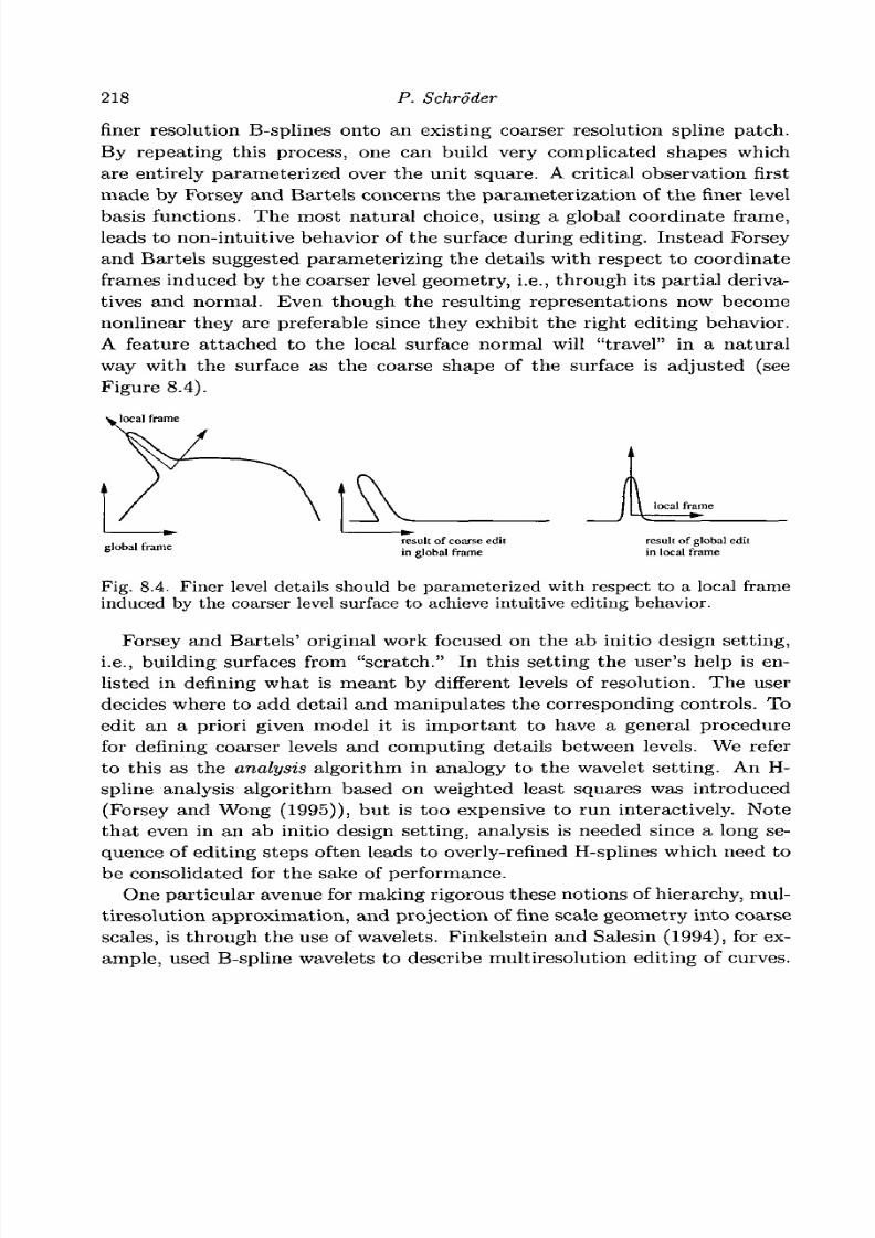
8/3/2019 Multivariate Approximation
http://slidepdf.com/reader/full/multivariate-approximation 228/296
218 P. Schroder
finer resolution B-splines onto an existing coarser resolution spline patch.
By repeating this process, one can build very complicated shapes which
are entirely parameterized over the unit square. A critical observation firstmade by Forsey and Bartels concerns the param eterization of the finer level
basis functions. The most natural choice, using a global coordinate frame,
leads to non-intuitive behavior of the surface during editing. Instead Forsey
and Bartels suggested parameterizing the details with respect to coordinate
frames induced by the coarser level geometry, i.e., through its partial deriva-
tives and normal. Even though the resulting representations now become
nonlinear they are preferable since they exhibit the right editing behavior.
A feature attached to the local surface normal will "travel" in a natural
way with the surface as the coarse shape of the surface is adjusted (see
Figure 8.4).
b local frame
. k l f result of coarse edit result of global editglobal frame i n g | o b a l f r a m e j n | Q c a l fmmf.
Fig. 8.4. Finer level details should be parameterized with respect to a local frameinduced by the coarser level surface to achieve intuitive editing behavior.
Forsey and Bartels' original work focused on the ab initio design setting,
i.e., building surfaces from "scratch." In this setting the user's help is en-
listed in defining what is mean t by different levels of resolution. The user
decides where to add detail and manipulates the corresponding controls. To
edit an a priori given model it is important to have a general procedure
for defining coarser levels and com puting de tails between levels. We refer
to this as the analysis algorithm in analogy to the wavelet setting. An H-
spline analysis algorithm based on weighted least squares was introduced
(Forsey and Wong (1995)), bu t is too expensive to run interactively. Note
that even in an ab initio design setting, analysis is needed since a long se-
quence of editing steps often leads to overly-refined H-splines which need to
be consolidated for the sake of performance.
One particu lar avenue for making rigorous these notions of hierarchy, mul-
tiresolution approxim ation, and projection of fine scale geometry into coarse
scales, is through the use of wavelets. Finkelstein and Salesin (1994), for ex-
ample, used B-spline wavelets to describe multiresolution editing of curves.
8/3/2019 Multivariate Approximation
http://slidepdf.com/reader/full/multivariate-approximation 229/296
Chapter 8 Scalable algorithms in computer graphics 219
As in H-splines, parameterization of details with respect to a coordinate
frame induced by the coarser level approximation is required to get correctediting semantics. Gortler and Cohen (1995) pointed out that wavelet rep-
resentations of details tend to behave in undesirable ways during editing and
returned to a pure B-spline representation as used in H-splines. In general
we find that critically sampled representations tend to break down under
editing operations. One way to understand this is to consider the fact that
in a critically sampled wavelet setting there exists a very carefully tuned
balance between the low pass (scaling function) and high pass (wavelet) fil-
ters. One cancels the aliases of the other. When a curve is edited, however,this balance is disturbed in a nonlinear fashion because of the deformation
of the underlying frames which are attached to the curve. As a consequence
one observes in practice that the alias cancellation property is lost and unde-
sirable "wiggles" appear in the geometry. These problems can be remedied
through the use of overrepresentations such as Burt-Adelson type pyramids
(Burt and Adelson (1983)) (see Section 8.4).
All the approaches mentioned above rely on a setting which admits pa-
rameterization over a trivial domain such as the unit interval (curve editing)or the unit square. Carrying these ideas over into the arbitrary topology sur-
face framework is not straightforward. The first to do so were Lounsbery et
al. (1997) who exploited the connection between wavelets and subdivision to
define different levels of resolution for arb itrary topology geometry. While
subdivision provides the scaling functions, corresponding wavelets can be
constructed with the help of the lifting scheme (Sweldens (1996); Sweldens
and Schroder (1996); Schroder and Sweldens (1995)). The original construc-
tions were limited to polyhedral wavelets, i.e., those constructed with thehelp of interpo lating scaling functions such as linear splines or the limit fun-
ctions of the (modified) butterfly subdivision scheme (Dyn et al. (1990);
Zorin et al. (1996)). The latter is not as suitable for editing purposes be-
cause of negative weights in the subdivision m asks. During editing opera-
tions, when one adjusts ("pulls on") a control point, undesired ripples will
appear on the surface.
8.2.1 Goals
We are seeking a geometric representation which unifies the advantages of
the approaches discussed above and remedies their shortcomings. It should
address the arbitrary topology challenge, support hierarchical editing seman-
tics and span the spectrum from patches to finely detailed triangle meshes.
Subdivision surfaces based on generalizations of spline patches, combined

8/3/2019 Multivariate Approximation
http://slidepdf.com/reader/full/multivariate-approximation 230/296
220 P. Schroder
with detail based extensions as in the H-spline approach provide such a
representa tion. They provide a pa th from pa tches to fine meshes using asingle primitive (hierarchical triangle mesh), and support the pa tch-type se-
mantics of manipulation and finest-level-detail polyhedral edi ts equally well.
Because they are the limit of successive refinement, subdivision surfaces sup-
port multiresolution algorithms, such as level-of-detail rendering, compres-
sion, wavelets, and num erical multigrid in a na tural way. The basic computa-
tional kernels are simple, resulting in easy-to-implement and efficient codes.
Boundaries and features such as creases can also be included through modi-
fied rules (Hoppe et al. (1994); Schweitzer (1996); DeRose et al. (1998); Levin(1999)), reducing the need for trimming curves. Even though the surfaces
are of arbitrary topology they possess simple parameterizations and efficient
algorithms exist for exact evaluation of values and derivatives of the limit
surface at arbitrary parameter locations (Stam (1998)). The main challenge
is to make the basic algorithms fast enough to escape the exponential time
and space growth of naive subdivision.
8.2.2 Notation
Before beginning with the description of the details of our algorithms we
fix some notatio n. We need enough machinery to talk about meshes both
in terms of their topology and geometry, i.e., their embedding in R3. For
this purpose it is useful to carefully distinguish between the topological and
geometric information. We denote a triangle mesh as a pair (P,IC): where
V is a set of N point positions pa = (xa, ya, za) £ R3
with 1 < a < N, and
/C is an abstract simplicial complex which contains all the topological, i.e.,adjacency information. The complex K, is a set of subsets of { 1 , . . . ,N}.
These subsets are called simplices and come in 3 types: vertices v = {a} €
V C IC; edges e = {a, 6} € E C /C; and faces / = {a , b, c} G T C IC, so that
any non-empty subset of a simplex of K. is again a simplex of IC, e.g., if a
face is present then so are its edges and vertices.
Let 6i denote the stand ard ith basis vector in R . For each simplex
s, its topological realization \s\ is the strictly convex hull of {6i \ i £ s} .
Thus | {a}| = 8a, |{a, 6}| is the open line segment between 6a and 6b, and\{a, b, c}\ is an open equilateral triangle. The topological realization \JC\
is defined as (JseJtlsl- The geometric realization <p(\IC\) relies on a linear
map ip : RN —> R3
defined by tp(Sa) = pa. Abusing notation a bit we
will abbreviate the geometric realization by writing pa = p(a) below. The
resulting polyhedron consists of points, segments, and triangles in R3.
Two vertices {a} and {b} are neighbors if {a, b} 6 E. A set of vertices is

8/3/2019 Multivariate Approximation
http://slidepdf.com/reader/full/multivariate-approximation 231/296
Chapter 8 Scalable algorithms in computer graphics 221
independent if no two vertices are neighbors. A set of vertices is maximally
independent if no larger independent set contains it (see Figure 8.18, left
side). The 1-ring neighborhood of a vertex {a} is the set
N{a) = {b\{a,b}£E}.
The outdegree Ka of a vertex is its number of neighbors. The star of a vertex
{a} is the set of simplices
star (a) = \^j s.
aEs, sEK.
We say that \}C\ is a two-dimensional manifold (or 2-manifold) with bound-
aries if for each a, |star(a)| is homeomorphic to a disk (interior vertex) or
half-disk (boundary vertex) in R2. An edge e = {a,b} is called a boundary
edge if there is only one face / with e C / .
8.3 Subdivision
For our purposes subdivision has two distinct components, one given bytopological operations on the simplicial complex and the other by opera-
tions on the geometric realization of the mesh, i.e., the association of a
point in 3D with every vertex in the complex. Starting with an initial mesh
(P°,/C° = {V°,E°,T0)) subdivision builds a new one {V
l,K>) by refin-
ing each face {a,b,c} G T° into four faces {a,ce,be}, {b, ae,ce}, {c, be,ae},
{ae,be,ce} € T1. The new vertices {ae}, {be}, {ce} 6 V1
can be thought of
as children of the edges across from the vertices {a}, {&}, {c} £ V°, respec-
tively. Continuing this construction recursively results in meshes (7-
>t
,/C
t
).The superscript i indicates the level of triangles and vertices, respectively.
The vertex sets are nested as VJ' C V* if j < i. We define odd vertices on
level i as M% = V l+1 \ V1. The set V l+1
consists of two disjoint sets: even
vertices ( V ) and odd vertices (M l). We define the level of a vertex a as the
smallest i for which a € V. The level of a is i + 1 if and only if a G M \
With each set V* we associate a geometric realization pl(a) e R
3, for all
a e V*. The set pl
contains all points on level i, pl
— {pz(a) \ a € V
1}.
Finally, a subdivision scheme is a linear operator 5 which takes the pointsfrom level i to points on the finer level i + 1: p
l+l= Sp
l, defining the
geometric realization at level i + 1.
Assuming that the subdivision converges, we can define a limit surface a
as
o= lim Skp°.
k
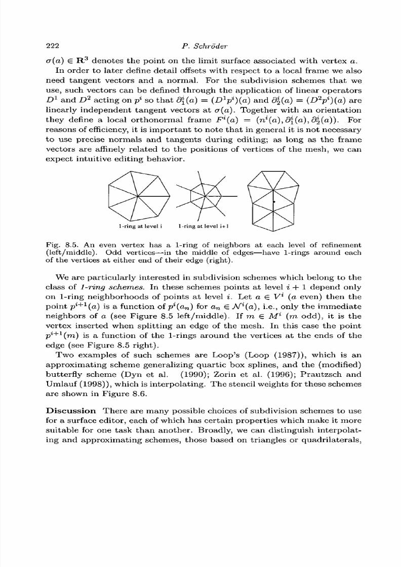
8/3/2019 Multivariate Approximation
http://slidepdf.com/reader/full/multivariate-approximation 232/296
222 P. Schroder
o(a) E R.3
denotes the point on the limit surface associated with vertex a.
In order to later define detail offsets with respect to a local frame we also
need tangent vectors and a normal. For the subdivision schemes that we
use, such vectors can be defined through the application of linear operators
D1
and D2 acting on p* so that d[(a) = (D
1p
i)(a) and <%(a) = (D
2p
i)(a) are
linearly independent tangent vectors at a (a). Together with an orientation
they define a local orthonormal frame Fl(a) = (n*(a) ,d\(a) ,^(a)) . For
reasons of efficiency, it is important to note that in general it is not necessary
to use precise normals and tangents during editing; as long as the frame
vectors are affinely related to the positions of vertices of the mesh, we can
expect intuitive editing behavior.
1-ring at level i 1-ring at level i+1
Fig. 8.5. An even vertex has a 1-ring of neighbors at each level of refinement(left/middle). Odd vertices—in the middle of edges—have 1-rings around eachof the vertices at either end of their edge (right).
We are particularly interested in subdivision schemes which belong to the
class of 1-ring schemes. In these schemes points at level i + 1 depend only
on 1-ring neighborhoods of points at level i. Let a € V1
(a even) then the
point pl+1
(a) is a function of pl
(an) for an € Nl
{a), i.e., only the immediateneighbors of a (see Figure 8.5 left/middle). If m 6 M
l(m odd), it is the
vertex inserted when splitting an edge of the mesh. In this case the point
pl+x
{m) is a function of the 1-rings around the vertices at the ends of the
edge (see Figure 8.5 right).
Two examples of such schemes are Loop's (Loop (1987)), which is an
approximating scheme generalizing quartic box splines, and the (modified)
butterfly scheme (Dyn et al. (1990); Zorin et al. (1996); Prautzsch and
Umlauf (1998)), which is interpolating. The stencil weights for these schemesare shown in Figure 8.6.
Discussion There are many possible choices of subdivision schemes to use
for a surface editor, each of which has certain properties which make it more
suitable for one task than another. Broadly, we can distinguish interpolat-
ing and approximating schemes, those based on triangles or quadrilaterals,

8/3/2019 Multivariate Approximation
http://slidepdf.com/reader/full/multivariate-approximation 233/296
Chapter 8 Scalable algorithms in computer graphics
Loop Stencils Butterfly Stencil
-1 2 -1
-1 2 -1
223
Fig. 8.6. Stencils for Loop subdivision with unnormalized weights for even and oddvertices (left) and for the regular butterfly (right). Note that the butterfly scheme,
since it is interpolating, only has a stencil for odd vertices.
as well as primal versus dual schemes. Interpola ting schemes such as the
butterfly scheme (Dyn et al. (1990); Zorin et al. (1996)) (triangles) or
Kobbelt's quad scheme (Kobbelt (1996a)) have the advantage that any ver-
tex has only one associated point, which is a sample of the limit surface.
This simplifies the implementation and makes adaptive subdivision partic-
ularly easy. For exam ple, it suffices to place a simple restric tion criterion
on the quadtrees that hold the point positions. A disadvantage of interpo-
lating schemes arises from the fact that the fundamental solutions of the
subdivision process by necessity have negative lobes. As a consequence the
surface develops oscillations when a control point is moved. In general, in-
terpolating schemes tend to produce surfaces which lack fairness and can
respond in non-intuitive ways when a user manipulates the control points.
An exception are variational subdivision schemes (Kobbelt (1996b)) which
are defined to produce fair surfaces th at are also interpolating. Unfortu-
nately they are com putationally intensive, as each subdivision s tep requires
the inversion of a (sparse) system of linear equations. Additionally it is not
clear how to support adaptive subdivision in this setting.
In contrast approximating schemes, which are largely based on general-
izations of splines, such as Loop (1987), Catmull-Clark (Catmull and Clark
(1978)), and Doo-Sabin (Doo and Sabin (1978)) tend to result in much
nicer editing behavior. Since the basis functions do not exhibit any undu-
lations, pulling on a control point results in a smooth, bump-like surface
change. Implementation of these schemes is slightly more involved as each
vertex now has to hold a number of point positions, one for every level of
the subdivision process on which it exists. For an efficient implem entation
this requires dynamically adjustable storage at each vertex. Adaptive sub-
division is still possible through the use of a restriction criterion, but care
must be taken to reference the point position at the proper level. Alterna-
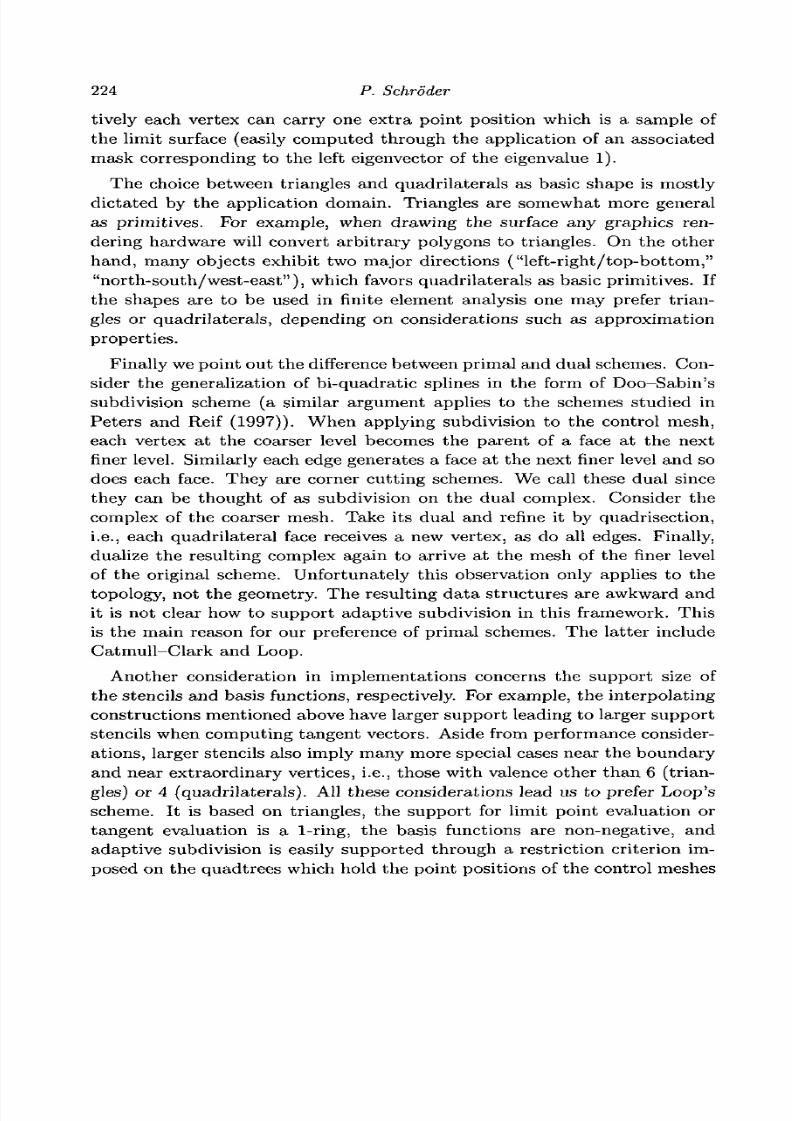
8/3/2019 Multivariate Approximation
http://slidepdf.com/reader/full/multivariate-approximation 234/296
224 P. Schroder
tively each vertex can carry one extra point position which is a sample of
the limit surface (easily computed through the application of an associated
mask corresponding to the left eigenvector of the eigenvalue 1).
The choice between triangles and quadrilaterals as basic shape is mostly
dictated by the application dom ain. Triangles are somewhat more general
as primitives. For example, when drawing the surface any graphics ren-
dering hardware will convert arbitrary polygons to triangles. On the other
hand , many objects exhibit two major directions ("left-right/top-bo ttom,"
"north-south/w est-ea st"), which favors quadrilaterals as basic primitives. If
the shapes are to be used in finite element analysis one may prefer trian-gles or quadrilaterals, depending on considerations such as approximation
properties.
Finally we point out the difference between primal and dual schemes. Con-
sider the generalization of bi-quadratic splines in the form of Doo-Sabin's
subdivision scheme (a similar argument applies to the schemes studied in
Peters and Reif (1997)). When applying subdivision to the control mesh,
each vertex at the coarser level becomes the parent of a face at the next
finer level. Similarly each edge generates a face at the next finer level and sodoes each face. They are corner cutting schemes. We call these dual since
they can be tho ugh t of as subdivision on the dual complex. Consider th e
complex of the coarser mesh. Take its dual and refine it by quadrisection,
i.e., each quadrilatera l face receives a new vertex , as do all edges. Finally,
dualize the resulting complex again to arrive at the mesh of the finer level
of the original scheme. Unfortunately this observation only applies to the
topology, not the geometry. The resulting data structures are awkward and
it is not clear how to supp ort adap tive subdivision in this framework. Thisis the main reason for our preference of primal schemes. The latter include
Catmull-Clark and Loop.
Another consideration in implementations concerns the support size of
the stencils and basis functions, respectively. For example, the interpolating
constructions mentioned above have larger support leading to larger sup port
stencils when computing tangent vectors. Aside from performance consider-
ations, larger stencils also imply many more special cases near the boundary
and near extraordinary vertices, i.e., those with valence other than 6 (trian-
gles) or 4 (quadrilaterals). All these considerations lead us to prefer Loop's
scheme. It is based on triangles, the support for limit point evaluation or
tangent evaluation is a 1-ring, the basis functions are non-negative, and
adaptive subdivision is easily supported through a restriction criterion im-
posed on the quadtrees which hold the point positions of the control meshes

8/3/2019 Multivariate Approximation
http://slidepdf.com/reader/full/multivariate-approximation 235/296
Chapter 8 Scalable algorithms in computer graphics 225
at different levels of resolution. The latter is particularly critical in escaping
the exponent ia l t ime and memory growth of naive subdivis ion.
8.4 Multiresolution extensions of subdivision
Using subdivision alone one could easily build a very efficient geometric
modeling system. The user manipulates the coarsest level control points
and thus shapes the limit surface. Suitably high performance can be deliv-
ered through the use of adaptive subdivision, for example, allocating larger
triangles in areas which are relatively flat and smaller triangles in areas of
high curvature . Figure 8.7 shows an instance of such adapta tion which is
natura lly supported by the recursive natu re of subdivision. Simply stop a
particular branch of the recursion when a local approximation criterion has
been satisfied. These criter ia can also be varied across the surface so as
to allocate resources in regions of particular interest without compromising
overall performance (see Figure 8.8).
Fig. 8.7. Subdivision describes a sm ooth surface as the limit of a sequence of refinedpolyhedra. The meshes show several levels of an adaptive Loop surface.
The capabil i t ies of such an edit ing system as presented to the user are very
similar to what one would f ind in more t radi t ional patch-based modelers ,
the only difference being that the system can deal with arbitrary topology
surfaces and no t ju s t those descr ibable over a tensor prod uc t dom ain. W h at
is missing is th e ab ility to define d eta il at m an y different levels of a hierarch y.
Fig ure 8.9 shows an exam ple of the head of Arm adil lo m an . Here the top
level control points were subdivided four t imes, yielding the surface on the
left side. I t is very sm oo th as one would expe ct . W h a t th e designe r would
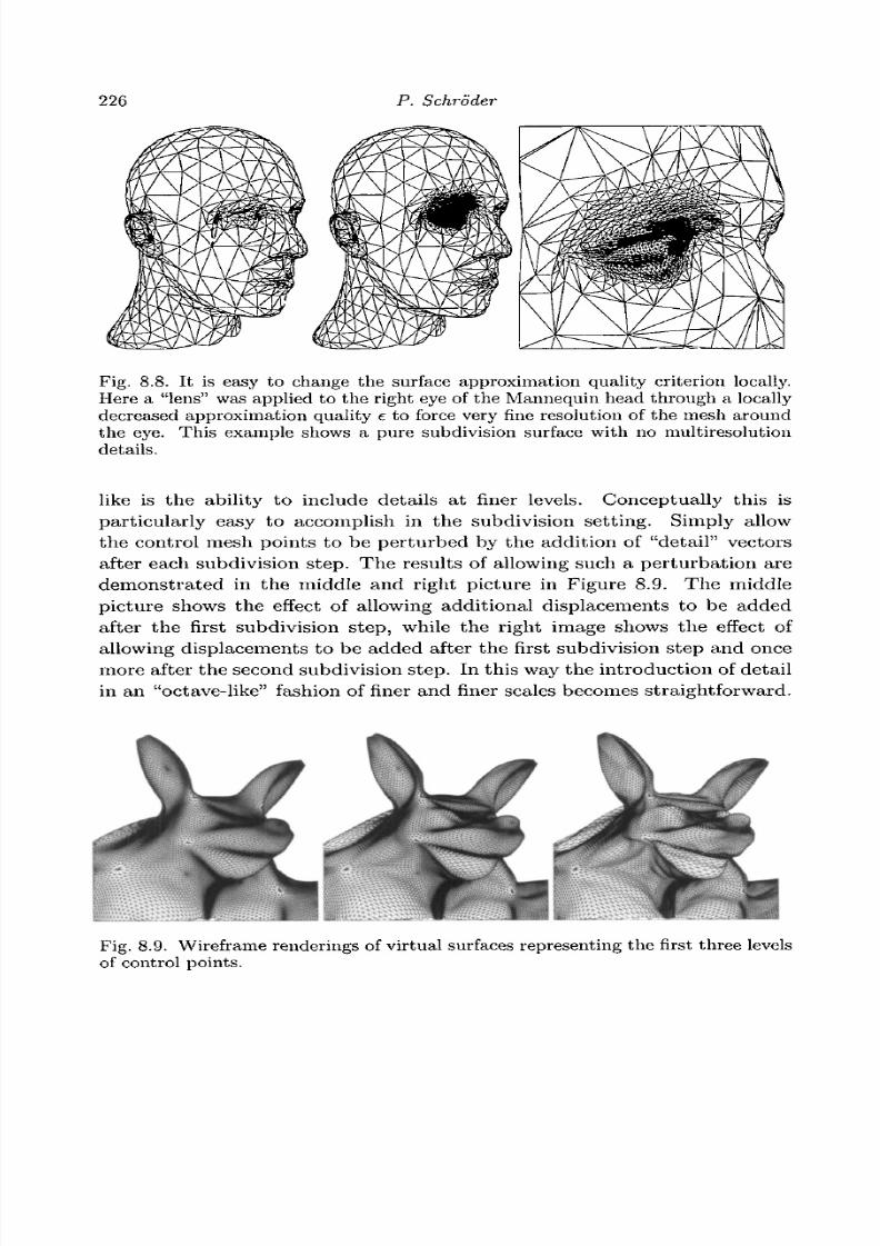
8/3/2019 Multivariate Approximation
http://slidepdf.com/reader/full/multivariate-approximation 236/296
226 P. Schroder
Fig. 8.8. It is easy to change the surface approximation quality criterion locally.Here a "lens" was applied to the right eye of the Mannequin head through a locallydecreased approximation quality e to force very fine resolution of the mesh aroundthe eye. This example shows a pure subdivision surface with no multiresolutiondetails.
like is the ability to include details a t finer levels. Conceptually this isparticularly easy to accomplish in the subdivision setting. Simply allow
the control mesh points to be perturbed by the addition of "detail" vectors
after each subdivision step. The results of allowing such a perturbation are
dem onstrated in the middle and right picture in Figure 8.9. The middle
picture shows the effect of allowing additional displacements to be added
after the first subdivision step, while the right image shows the effect of
allowing displacements to be added after the first subdivision step and once
more after the second subdivision step. In this way the introduction of detail
in an "octave-like" fashion of finer and finer scales becomes straightforward.
Fig. 8.9. Wireframe renderings of virtual surfaces representing the first three levelsof control points.

8/3/2019 Multivariate Approximation
http://slidepdf.com/reader/full/multivariate-approximation 237/296
Chapter 8 Scalable algorithms in computer graphics 227
To put these ideas on a solid basis we must discuss the analysis operator.
Subdivision, or synthesis, goes from coarse to fine, while analysis goes from
fine to coarse and computes the detail vectors. We first need smoothing and
downsampling, i.e., a linear operation H to build a smooth coarse mesh at
level i — 1 from a fine mesh at level i:
Several options are available here.
• Least squares One could define analysis to be optimal in the least
squares sense,
The solution may have unwanted undulations and is too expensive to
compute interactively (Forsey and Wong (1995)).
• Fairing A coarse surface could be obtained as the solution to a global
variational problem. This is too expensive as well. An alterna tive is
presented by Taubin (1995), who uses a local smoothing approach.Because of its com putational simplicity we decided to use a version of Taubin
smoothing. As before let a € V1
have K neighbors a^ £ V1. Use the
average, p'(v) — K~l
X^=iP*(afc)j to define the discrete Laplacian C{a) =
pl{v) — p
l(a). On this basis Taubin gives a Gaussian-like smoother with
reduced shrinkage problems
# : = ( / + / * £ )( / + A £ ),
with /z and A tuned to ameliorate the shrinkage problem inherent in straight
Gaussian smoothing (Taubin (1995)). With subdivision and smoothing in
place, we can describe the transform needed to support multiresolution edit-
ing.
Recall that for multiresolution editing we want the difference between
successive levels expressed with respect to a frame induced by the coarser
level, i.e., the offsets are relative to the smoother level. With each vertex
a and each level i > 0 we associate a detail vector, dl(a) € R 3 . The set d
l
contains all detail vectors on level i, d l = {d l(a) | a £ V1}. As indicated in
Figure 8.10 the detail vectors are defined as
d* = [F l)T(P* - Sv'-1) = (F'f (I - SH)p\
i.e., the detail vectors at level i record how much the points at level i differ
from the result of subdividing the points at level i — 1. This difference is

8/3/2019 Multivariate Approximation
http://slidepdf.com/reader/full/multivariate-approximation 238/296
228 P. Schroder
Smoothing Subdivision
Fig. 8.10. Wiring diagram of the multiresolution transform.
Fig. 8.11. Analysis propagates the changes on finer evels to coarser levels, keepingthe magnitude of details under control. Left: The initial mesh. Center: A simpleedit on level 3. Right: The effect of the edit on level 2. A significant part of thechange was absorbed by higher level details.
then represented with respect to the local frame Fl to obtain coordinate
independence.
Since detail vectors are sampled on the fine level mesh V1, this transforma-
tion yields an overrepresentation in the spirit of the Burt-Adelson pyramid
(Burt and Adelson (1983)). The only difference is that the smoothing filter
(Taubin) is not th e dual of the subdivision filter (Loop). Theoretically it
would be possible to subsample the detail vectors and only record a detail
per odd vertex (elements of Ml~
l). This is what happens in the wavelet
transform. However, subsampling the details severely restric ts the family
of smoothing operators that can be used and is not desirable in an editing
environment in either case (see our comments in Section 8.2).
Figure 8.11 shows an exam ple of analysis applied to a shape with a stron g
feature at a fine level. This feature yields details at coarser levels which are
smoothed versions of the finer level feature.
Figure 8.12 shows two triangle mesh approximations of the Armadillo head
with multiresolution details. Approximately the same number of triangles
are used for the adaptive and uniform mesh. The adaptive rendering took
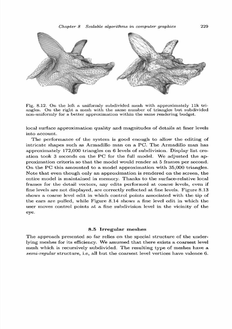
8/3/2019 Multivariate Approximation
http://slidepdf.com/reader/full/multivariate-approximation 239/296
Chapter 8 Scalable algorithms in com puter graphics 229
Fig. 8.12. On the left a uniformly subdivided mesh with approximately Ilk tri-angles. On the right a mesh with the same number of triangles but subdividednon-uniformly for a better approximation within the same rendering budget.
local surface approximation quality and magnitudes of details at finer levels
into account.The performance of the system is good enough to allow the editing of
intricate shapes such as Armadillo man on a PC. The Armadillo man has
approxim ately 172,000 triangles on 6 levels of subdivision. Display list cre-
ation took 3 seconds on the P C for the full model. We adjusted the ap-
proximation criteria so that the model would render at 5 frames per second.
On the PC this amounted to a model approximation with 35,000 triangles.
Note that even though only an approximation is rendered on the screen, the
entire model is maintained in memory. Thanks to the surface-relative localframes for the detail vectors, any edits performed at coarse levels, even if
fine levels are not displayed, are correctly reflected at fine levels. Figure 8.13
shows a coarse level edit in which control points associated with the tip of
the ears are pulled, while Figure 8.14 shows a fine level edit in which the
user moves control points at a fine subdivision level in the vicinity of the
eye.
8.5 Irregular meshes
The approach presented so far relies on the special structure of the under-
lying meshes for its efficiency. We assumed th at the re exists a coarsest level
mesh which is recursively subdivided. The resulting type of meshes have a
semi-regular structure, i.e, all but the coarsest level vertices have valence 6.

8/3/2019 Multivariate Approximation
http://slidepdf.com/reader/full/multivariate-approximation 240/296
230 P. Schroder
Fig. 8.13. An example of a coarse level edit in which a group of control points atthe tip of the ears is pulled up and then subsequently only the control points atthe tip of one ear are pushed down. Note that fine level detail on the shape movesalong with the surface as one would intuitively expect.
Fig. 8.14. An example of a fine level edit. Here control points at the third subdi-vision level are exposed and the user selects a group of them around the eye lid,
affecting only a very small region around the eye.
When geometry is built "from scratch" it is an easy matter to enforce this
requirement. The situation changes when one wants to work with an arbi-
trary input mesh coming from some other application. For example, meshes
coming from 3D acquisition devices typically are completely unstructured,
or irregular. If we wish to apply multiresolution analysis and associated
algorithms to these we must first convert them to semi-regular meshes, orremesh them. A first step in such a procedure, and for that matter in many
other numerical algorithms which aim to deal with such meshes, is the es-
tablishment of a smooth parameterization. In a very fundamental sense we
are seeking methods of building a proper manifold structure, i.e., charts and
an atlas, for such settin gs. While an arbit rary triangle mesh can always
be thought of as parameterized over itself this is not a useful observation

8/3/2019 Multivariate Approximation
http://slidepdf.com/reader/full/multivariate-approximation 241/296
Chapter 8 Scalable algorithms in computer graphics 231
Fig. 8.15. Overview of the remeshing algorithm. Top left: a scanned input mesh(courtesy Cyberware). Next the parameter or base domain, obtained through meshsimplification. Top right: regions of the original mesh colored according to their
assigned base domain triangle. Bottom left: adaptive remeshing with subdivisionconnectivity (e = 1%). Bottom right: multiresolution edit.
in practice: a mesh which consists of hundreds of thousands of triangles is
trivially parameterized over its combinatorial complex using the geometric
realization <p. But this object is unwieldy and not smooth (piecewise linear
only). W hat we seek instead is a parame terization of the original mesh over
a homeomorphic complex with very few triangles. Once the original mesh,
or a close approximation to it, is realized in this fashion many numerical
modeling tasks are greatly facilitated. In particular it is then an easy mat-
ter to resample the original mesh onto a semi-regular mesh as it appears in
traditional subdivision, allowing us to apply the algorithms described in the
previous section.
A procedure for establishing such a param eterization is the subject of this
section. Figure 8.15 shows the outline of the procedure: beginning with an
irregular input mesh (top left), in a first step a base domain is established
through mesh simplification (top middle). Concurrent with simplification,
a mapping is constructed which assigns every vertex from the original mesh
to a base triangle (top right). Using this mapping an adaptive remesh with
subdivision connectivity can be built (bottom left) which is now suitable for
such applications as multiresolution editing (bottom middle).
There are many possible ways of approaching this problem and before

8/3/2019 Multivariate Approximation
http://slidepdf.com/reader/full/multivariate-approximation 242/296
232 P. Schroder
describing the details of one such algorithm we first consider some other
possibilities. These fall into two broad categories: those that are geared to-
wards approximating an initial unstructured mesh with smooth patches; and
those which explicitly aim at constructing parameterizations for remeshing.
8.5.1 Approx imation of a given set of samples
Hoppe and co-workers (Hoppe et al. (1994)) describe a fully automatic al-
gorithm for approximating a given polyhedral mesh with (modified) Loop
subdivision patches (Loop (1987)) respecting features such as edges and cor-
ners. Their algorithm uses a nonlinear optimization procedure taking into
account approximation error and the number of triangles of the base do-
main. The result is a smooth parameterization of the original polyhedral
mesh with a (hopefully) small number of patches. Since the approach only
uses subdivision, small features in the original mesh can only be resolved
accurately by increasing the number of patches accordingly. From the point
of view of constructing parameterizations, the main drawback of algorithms
in this class is that the number of triangles in the base domain depends
heavily on the geometric complexity of the original surface.
This latter problem was addressed in work of Krishnamurthy and Levoy
(1996). They approximate densely-sampled geometry with bi-cubic spline
patches and displacement maps. Arguing that a fully automatic system can-
not put isoparameter lines where a skilled modeler or animator would want
them, they require the user to lay out the entire network of top level spline
patch boundaries . A coarse-to-fine matching procedure with relaxation is
used to arrive at a high quality patch-based surface whose base domain need
not mimic small scale geometric features. Any fine level features a re cap-
tured by allowing the addition of a displacement map on top of the smooth
spline patches. The principal drawback of their procedure is that the user
is required to define the entire base domain rather then only selected fea-
tures. Additionally, given that the procedure works from coarse to fine, it
is possible for the procedure to "latch" onto the wrong part of the surface
in regions of high curvature (Krishnamurthy and Levoy (1996), Figure 7).
8.5.2 Remeshing
Lounsbery and co-workers (Lounsbery (1994); Lounsbery et al. (1997)) were
the first to propose algorithms that extend classical multiresolution analysis
to arb itrary topology surfaces. Because of its connection to the m athe-
matical foundations of wavelets, this approach has proven very attractive
8/3/2019 Multivariate Approximation
http://slidepdf.com/reader/full/multivariate-approximation 243/296
Chapter 8 Scalable algorithms in computer graphics 233
(Schroder and Sweldens (1995); Eck et al. (1995); Zorin et al. (1996); Eck
and Hoppe (1996); Certain et al. (1996); Zorin et al. (1997)). The algorithm
described in the first half of this chapter belongs to this class. Since the cen-
tral requirement of these methods is that the input mesh have subdivision
connectivity-remeshing is generally required to apply these approaches. Eck
and co-workers (Eck et al. (1995)) were the first to develop such a remeshing
algorithm, computing a smooth parameterization of high resolution triangle
meshes over a low face-count base domain, followed by a semi-regular resam-
pling step. After this conversion step, adaptive simplification, compression,
progressive transmission, rendering, and editing become simple and efficient
operations (Certain et al. (1996); Eck and Hoppe (1996); Zorin et al. (1997)).
Eck et al. arrive at the base domain through a Voronoi tiling of the orig-
inal mesh. Using a sequence of local harmonic maps, a parameterization
which is smooth over each triangle in the base domain and which meets with
C° continuity at base domain edges is constructed (Eck et al. (1995), Plate
l(f)). Runtimes for the algorithm can be long because of the many harmonic
map computations. This problem was recently addressed by Duchamp and
co-workers (Duchamp et al. (1997)), who reduced the harmonic map com-
putations from their initial O(N2) complexity to O(N log N) through hi-
erarchical preconditioning.! The initial Voronoi tile construction relies on
a number of heuristics which render the overall algorithm fragile (for an
improved version see Klein et al. (1997)). Moreover, there is no explicit
control over the number of triangles in the base domain or the placement
of patch boundaries. The latter is critical in applications as one wants to
avoid unnecessary subdivision near sharp features.
8.5.3 An alternative parameterization algorithm
We describe here an algorithm which was designed to overcome the draw-
backs of previous work as well as to introduce new features. A fast coarsi-
fication strategy is used to define the base domain, avoiding the potential
difficulties of finding Voronoi tiles (Eck et al. (1995); Klein et al. (1997)).
Since the algorithm proceeds from fine to coarse, correspondence problems
found in coarse-to-fine strategies (Krishnamurthy and Levoy (1996)) are
avoided, and all features are correctly resolved. Piecewise linear approxima-
tions to conformal maps are used during coarsification to produce a global
parameterization of the original mesh. This map is then further improved
through the use of a hierarchical Loop smoothing procedure obviating the
f The hierarchy construction they employed for use in a multigrid solver is closely related to thehierarchy construction described below.
8/3/2019 Multivariate Approximation
http://slidepdf.com/reader/full/multivariate-approximation 244/296
234 P. Schroder
need for iterative numerical solvers (Eck et al. (1995)). Since the procedure
is performed globally, derivative discontinuities at the edges of the base do-
main are avoided (Eck et al. (1995)). In contrast to fully automatic methods
(Eck et al. (1995)), the algorithm supports vertex and edge tags (Hoppe et
al. (1994)) to constrain the final parameterization to align with selected fea-
tures; however, the user is not required to specify the entire patch network
(Krishnamurthy and Levoy (1996)). During remeshing we take advantage of
the original fine-to-coarse simplification hierarchy to output a sparse, adap-
tive, semi-regular mesh directly without resorting to a depth-first oracle
(Schroder and Sweldens (1995)) or the need to produce a uniform subdivi-
sion connectivity mesh at exponential cost followed by wavelet thresholding
(Certain et al. (1996)).
8.6 Hierarchical surface representation
An important part of the algorithm is the construction of a mesh hierar-
chy. The original mesh (P,/C) = ( 7 ' i , /C i) is successively simplified into a
series of homeomorphic meshes (P',/C') with 0 < I < L, where (V0,IC
0) is
the coarsest or base mesh (see Figure 8.16). Several approaches for such a
mesh simplification have been proposed, most notably progressive meshes
(PM) (Hoppe (1996)). In PM the basic operation is the "edge collapse."
A sequence of such atomic operations is prioritized based on approximation
error. The linear sequence of edge collapses can be partially ordered based
on topological dependence (Xia and Varshney (1996); Hoppe (1997)), which
defines levels in a hierarchy. The depth of these hierarchies appears "reason-
able" in practice, though can vary considerably for the same dataset (Hoppe
(1997)).
Our approach is similar in spirit, but inspired by the hierarchy proposed
by Dobkin and Kirkpatrick (1985) (DK), which guarantees that the num-
ber of levels L is O(\ogN). While the original DK hierarchy is built for
convex meshes, we show how the idea behind DK can be used for general
ones. The DK atomic simplification step is avertex remove,
followed by aretriangulation of the hole. The two basic operations "vertex remove" and
"edge collapse" are related since an edge collapse into one of its endpoints
corresponds to a vertex removal with a particular retriangulation of the re-
sulting hole (see Figure 8.17). The inain reason for choosing an algorithm
based on the ideas of the DK hierarchy is that it guarantees a logarithmic
bound on the number of levels.

8/3/2019 Multivariate Approximation
http://slidepdf.com/reader/full/multivariate-approximation 245/296
Chapter 8 Scalable algorithms in computer graphics
Original mesh (level 14)
235
Fig. 8.16. Exam ple of a modified DK m esh hierarchy. At the top the finest (original)mesh (/jd/C^I) followed by an intermediate mesh, and the coarsest (base) mesh</?(|/C°|) at the bottom (original dataset courtesy University of Washington).
8.6.1 Vertex removal
One DK simplification step K} —> K}~x
consists of removing a maximally
independent set of vertices with low outdegree (see Figure 8.18). Recall
that an independent set of vertices has the property that no two vertices
in the set are connected by an edge. To find such a set, the original DK
algorithm used a greedy approach based only on topological information.
Instead it is desirable to take geometric information into account as well.
This can be done by selecting candidates for the independent set based on
a priority queue.
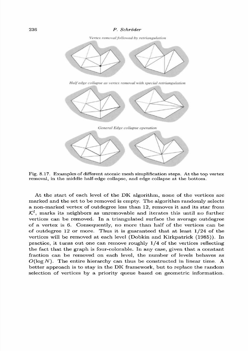
8/3/2019 Multivariate Approximation
http://slidepdf.com/reader/full/multivariate-approximation 246/296
236 P. Schroder
Vertex rem oval followed by retriangulation
Half edge collapse as vertex removal with special retriangulation
General Edge collapse operation
Fig. 8.17. Examples of different a tom ic mesh simplification steps. At the top vertexremoval, in the middle half-edge collapse, and edge collapse at the bottom.
At the start of each level of the DK algorithm, none of the vertices are
marked and the set to be removed is empty. The algorithm randomly selects
a non-marked vertex of outdegree less than 12, removes it and its star from
K,1, marks its neighbors as unremovable and iterates this until no further
vertices can be removed. In a triangulated surface the average outdegree
of a vertex is 6. Consequently, no more than half of the vertices can be
of outdegree 12 or more. Thus it is guaranteed tha t at least 1/24 of the
vertices will be removed at each level (Dobkin and Kirkpatrick (1985)). Inpractice, it turns out one can remove roughly 1/4 of the vertices reflecting
the fact that the graph is four-colorable. In any case, given that a constant
fraction can be removed on each level, the number of levels behaves as
O(\ogN). The entire hierarchy can thus be constructed in linear time. A
better approach is to stay in the DK framework, but to replace the random
selection of vertices by a priority queue based on geometric information.
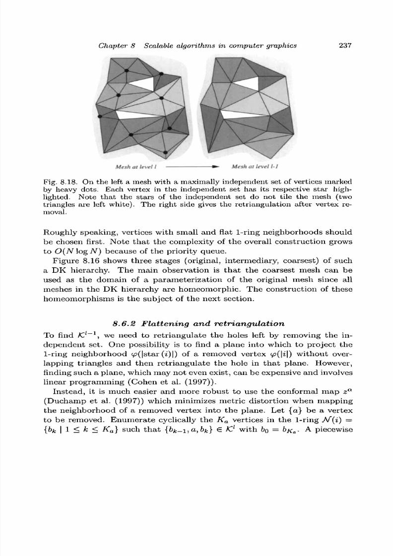
8/3/2019 Multivariate Approximation
http://slidepdf.com/reader/full/multivariate-approximation 247/296
Chapter 8 Scalable algorithms in computer graphics 237
Mesh at level I • - Mesh at level I-1
Fig. 8.18. On the left a mesh with a maximally independent set of vertices markedby heavy dots. Each vertex in the independent set has its respective star high-lighted. Note tha t the stars of the independent set do not tile the mesh (twotriangles are left white). The right side gives the retriangulation after vertex re-moval.
Roughly speaking, vertices with small and flat 1-ring neighborhoods should
be chosen first. Note that the complexity of the overall construction grows
to O(N log N) because of the priority queue.
Figure 8.16 shows three stages (original, intermediary, coarsest) of such
a DK hierarchy. The main observation is that the coarsest mesh can be
used as the domain of a parameterization of the original mesh since all
meshes in the DK hierarchy are homeomorphic. The construction of these
homeomorphisms is the subject ofthe
next section.
8.6.2 Flattening and retriangulation
To find K}~^, we need to retriangulate the holes left by removing the in-
dependent set. One possibility is to find a plane into which to project the
1-ring neighborhood v?(|star (i)\) of a removed vertex <p(\i\) without over-
lapping triangles and then retriangulate the hole in that plane. However,
finding such a plane, which may not even exist, can be expensive and involves
linear programming (Cohen et al. (1997)).
Instead, it is much easier and more robust to use the conformal map za
(Duchamp et al. (1997)) which minimizes metric distortion when mapping
the neighborhood of a removed vertex into the plane. Let {a} be a vertex
to be removed. Enumerate cyclically the Ka vertices in the 1-ring Af(i) =
{bk | 1 < k < Ka} such that {bk-i,a,bk} 6 K} with 6Q = bxa. A piecewise
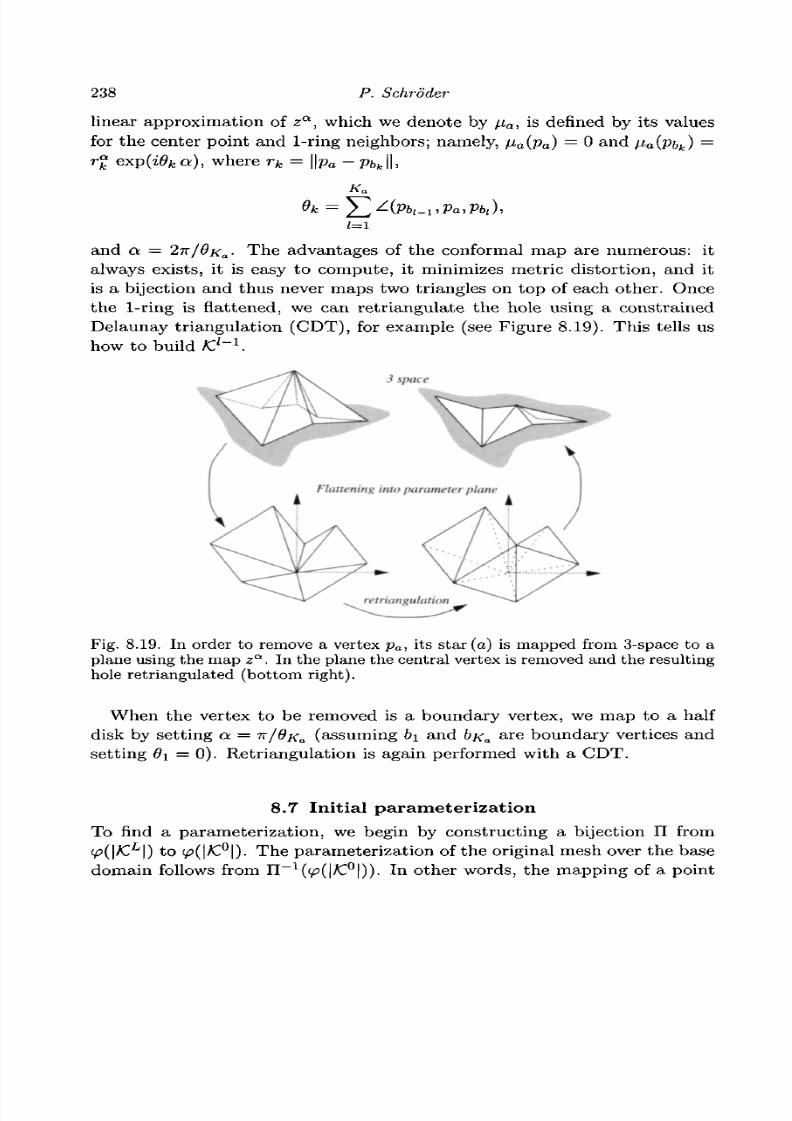
8/3/2019 Multivariate Approximation
http://slidepdf.com/reader/full/multivariate-approximation 248/296
238 P. Schroder
linear approximation of za, which we denote by na, is defined by its values
for the center point and 1-ring neighbors; namely, na{pa) = 0 and fJ,a(Pbk) =
), where rk = \\pa-P bk\\ ,
1= 1
and a = 2TT/9na • The advantages of the conformal map are numerous: it
always exists, it is easy to compute, it minimizes metric distortion, and it
is a bijection and thus never maps two triangles on top of each other. Once
the 1-ring is flattened, we can retriangulate the hole using a constrainedDelaunay triangulation (CDT), for example (see Figure 8.19). This tells us
how to build /C'"1.
3 space
Flattening into parameter plane
retriangulation
Fig. 8.19. In order to remove a vertex pa, its star (a) is mapped from 3-space to aplane using the map z
a. In the plane the central vertex is removed and the resulting
hole retriangulated (bottom right).
When the vertex to be removed is a boundary vertex, we map to a half
disk by setting a = 7r/0/co (assuming b\ and bxa are boundary vertices and
setting 6\ =0) . Retriangulation is again performed with a CDT.
8.7 Initial parameterization
To find a parameterization, we begin by constructing a bijection II from
(p{\K,L\) to (/J(|/C°|). The parameterization of the original mesh over the base
domain follows from Tl~ l{ip(\K?\)). In other words, the mapping of a point

8/3/2019 Multivariate Approximation
http://slidepdf.com/reader/full/multivariate-approximation 249/296
Chapter 8 Scalable algorithms in computer graphics 239
p £ (^(|/CL|) through II is a point p° = U.(a) G </J(|/C°|), which can be wri t ten
asp° =
where {a, b, c} €. /C° is a face of the base domain and a, P and 7 are barycen-
tric coordinates, i.e., a + P + 7 = 1.
The mapping can be computed concurrently with the hierarchy construc-
tion . The basic idea is to successively compute piecewise linear bijections
IT' between <^(|/CL|) and ip(\K,
l\) starting with II^, which is the identity, and
ending with II
0
= IT.Notice that we only need to compute the value of II' at the vertices of
/C^. At any other point it follows from piecewise linearity, f Assume we are
given Pi' and want to compute IT'"1. Each vertex {a} 6 K.L falls into one of
the following categories:
(i) {a} € /Ci -1
: The vertex is not removed on level I and survives on level
l — l. In this case nothing needs to be done, n ' "1
^ ) = I I;(p a) = pa;
(ii) {a} €K.
1
\JC
l~
l:
The vertex gets removed when going from I to /—
1.Consider the flattening of the 1-ring around pa (see Figure 8.19).
After retriangulation, the origin lies in a triangle which corresponds
to some face t = {d, e, / } e K.l~x and has barycentric coordinates
(a,P,y) with respect to the vertices of that face, i.e., a^a{Pd) +
PMa(Pe) +7A*a(p/) (see Figure 8.20). In that case, let n '- 1
( p a ) =
apd + PPe + 7P/I
(iii) {a} 6 K,L
\K): The vertex was removed earlier, thus Il'(p tt ) =
a
1
Pa' + P'Pb' + j'Pc' for some triangle t' = {a',6',c'} e K.
1
. Ift' € K}~1, nothing needs to be done; otherwise, the independent
set property guarantees that exactly one vertex of t' is removed,
say {a '} . Consider the conformal map / v (Figure 8.20). After
retriangulation, the na'(Pa) lies in a triangle which corresponds to
some face t = {d,e,f} € K1"
1with barycentric coordinates (a,/3,7)
(black dots within highlighted face in Figure 8.20). In that case, let
n ' ^ p a ) = apd + Ppe + ypj (i.e., all vertices in Figure 8.20 are
reparameterized in this way).
Note that on every level, the algorithm requires a sweep through all the
vertices of the finest level resulting in an overall complexity of O(N log N).
Figure 8.21 visualizes the mapping we jus t computed.
t In the vicinity of vertices in K l a triangle {a,b,c} 6 K.L can straddle multiple triangles in K.1.In this case the map depends on the flattening strategy used (see Section 8.6.2).

8/3/2019 Multivariate Approximation
http://slidepdf.com/reader/full/multivariate-approximation 250/296
240 P. Schroder
assign barycentric
coordinates to oldpoint in new triangle
Fig. 8.20. After retriangulation of a hole in the plane (see Figure 8.19), the justremoved vertex gets assigned barycentric coordinates with respect to the containingtriangle on the coarser level. Similarly, all the finest level vertices that were mappedto a triangle of the hole now need to be reassigned to a triangle of the coarser level.
Fig . 8.21. Base dom ain <^(|/C°|). For each poin t pa from the original mesh, its
mapping II(p o) is shown with a dot on the base domain.
8.7.1 Tagging and feature lines
In the algorithm described so far, there is no a priori control over which
vertices end u p in the base dom ain or how they will be connected. However,
often there are features such as sharp creases in the input mesh. It is de-
sirable to ensure that these features align with particular isoparameter lines
in the param eterization. Such features could be detected automatically orspecified by the user. We consider two types of features on the finest mesh:
vertices and paths of edges. Guaranteeing that a certain vertex of the orig-
inal mesh ends up in the base domain is straightforward. Simply mark th at
vertex as unremovable throughout the DK hierarchy.
We now describe an algorithm for guaranteeing that a certain path of
edges on the finest mesh gets mapped to an edge of the base domain. Let
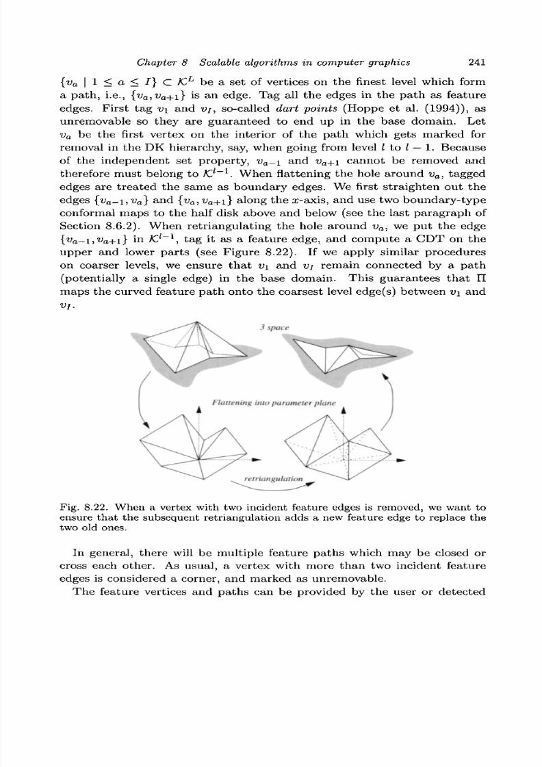
8/3/2019 Multivariate Approximation
http://slidepdf.com/reader/full/multivariate-approximation 251/296
Chapter 8 Scalable algorithms in computer graphics 241
{v a | 1 < a < 7} C K.L be a set of vertices on the finest level which form
a path, i.e., {v a,va+i} is an edge. Tag all the edges in the path as feature
edges. First tag v\ and vi, so-called dart points (Hoppe et al. (1994)), as
unremovable so they are guaranteed to end up in the base domain. Let
va be the first vertex on the interior of the path which gets marked for
removal in the DK hierarchy, say, when going from level I to I — 1. Because
of the independent set property, va-\ and va+\ cannot be removed and
therefore must belong to K}~ 1. When flattening the hole around va, tagged
edges are treated the same as boundary edges. We first straighten out the
edges {v a-i,va} and {v a, va+ i} along the x-axis, and use two boun dary-type
conformal maps to the half disk above and below (see the last paragraph of
Section 8.6.2). When retriangulating th e hole around va, we put the edge
{v a-i,va+i} in K.l~
l, tag it as a feature edge, and compute a CDT on the
upper and lower part s (see Figure 8.22). If we apply similar procedures
on coarser levels, we ensure that v\ and vj remain connected by a path
(potentially a single edge) in the base domain. This guarantees th at II
maps the curved feature path onto the coarsest level edge(s) between v\ and
VI .
3 space
Flattening into parameter plane
Fig. 8.22. When a vertex with two incident feature edges is removed, we want to
ensure that the subsequent retriangulation adds a new feature edge to replace thetwo old ones.
In general, there will be multiple feature paths which may be closed or
cross each othe r. As usual, a vertex with more than two incident feature
edges is considered a corner, and marked as unremovable.
The feature vertices and paths can be provided by the user or detected
8/3/2019 Multivariate Approximation
http://slidepdf.com/reader/full/multivariate-approximation 252/296
242 P. Schroder
automatically. As an example of the latter case, we consider every edge
whose dihedral angle is below a certain threshold to be a feature edge, and
every vertex whose curvature is above a certain threshold to be a feature
vertex. An example of this strategy is illustrated in Figure 8.25.
8.8 Remeshing
In this section, we consider remeshing using semi-regular triangulations. In
the process, we compute a smoothed version of our initial parameteriza-
tion. We also show how to efficiently construct an adaptive remesh withguaranteed error bounds.
8.8.1 Uniform remeshing
Since II is a bijection, we can use I I "1
to map the base domain to the original
mesh. We follow the strategy used in Eck et al. (1995), quadrisecting the
base domain and using the inverse map to obtain a semi-regular connectivity
remeshing. This introduces a hierarchy of semi-regular meshes (V m,K .m)(V is the point set and K, is the complex) obtained from m-fold midpoint
subdivision of the base domain (V°,K,°) = (V °:KP). Midpoint subdivision
implies that all new domain points lie in the base domain, Vm
C (£>(|£°|)
and \tm\ = \K.°\. All vertices of fc
m\it° have outdegree 6. The uniform
remeshing of the original mesh on level m is given by (U ~1{P m), K,m).
We thus need to compute Tl~ l(q) where q is a point in the base domain
with dyadic barycentric coordinates. In particular, we need to compute
which triangle of ipd^-^l) contains H~1(q), or, equivalently, which triangleof n^d^C^D) contains q. This is a standard point location problem in an
irregular triangulation. This problem can be solved with the point location
algorithm of Brown and Faigle (1997) which avoids looping that can occur
with non-Delaunay m eshes (Guibas and Stolfi (1985); Garland and Heckbert
(1995)). Once we have found the triangle {a,b,c} which contains q, we can
write q as
and thus
U~l(q) = aPa + pPb + 7 Pc € <p(\IC L\).
Figure 8.23 shows the result of this procedure: a level 3 uniform remeshing
of a 3-holed torus using the IT"1
map.
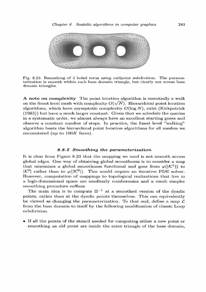
8/3/2019 Multivariate Approximation
http://slidepdf.com/reader/full/multivariate-approximation 253/296
Chapter 8 Scalable algorithms in computer graphics 243
Fig. 8.23. Remeshing of 3 holed torus using midpoint subdivision. The parame-terization is smooth within each base domain triangle, but clearly not across basedomain triangles.
A n o t e on c o m p l e x i t y The point locat ion algor i thm is essentially a walk
on the finest level mesh with complexity O(\/~N). Hierarchical point location
algor i thms, which have asymptot ic complexi ty O(\ogN), exist (Kirkpatrick
(1983)) but have a much larger constant . Given that we schedule the queries
in a systemat ic order , we almost always have an excellent start ing guess andobserve a cons tan t number of s teps . In pract ice , the finest level "walking"
algor i thm beats the hierarchical point locat ion algor i thms for all meshes we
encountered (up to WOK faces).
8.8.2 Smoothing the parameterization
It is clear from Figure 8.23 that the mapping we used is not smooth across
global edges. One way of obtaining global smoothness is to consider a map
that minimizes a global smoothness functional and goes from y?(|/CL|) to
\K?\ rather than to y>(|£°|). This would require an iterative PDE solver.
However, computation of mappings to topological realizations that live in
a high-dimensional space are needlessly cumbersome and a much simpler
smoothing procedure suffices.
The main idea is to compute n- 1
at a smoothed version of the dyadic
points, rather than at the dyadic points themselves. This can equivalently
be viewed as changing the parameterization. To that end, define a map £
from the base domain to itself by the following modification of classic Loop
subdivision.
• If all the points of the stencil needed for computing either a new point or
smoothing an old point are inside the same triangle of the base domain,

8/3/2019 Multivariate Approximation
http://slidepdf.com/reader/full/multivariate-approximation 254/296
244 P. Schroder
we can simply apply the Loop weights and the new points will be in that
same face.
• If the stencil stretches across two faces of the base domain, we flatten
them out using a "hinge" map at their common edge. We then compute
the point's position in this flattened domain and extract the triangle in
which the point lies together with its barycentric coordinates.
• If the stencil stretches across multiple faces, we use the conformal flatten-
ing strategy discussed earlier.
Note that the modifications to Loop force £ to map the base domain onto
the base domain. We emphasize th at we do not apply the classic Loop
scheme (which would produce a "blobby" version of the base domain). Nor
are the surface approximations that we later produce Loop surfaces.
The composite map IT"1
o £ is our smoo thed parameterization that maps
the base domain on to the original surface. The mth level of uniform remesh-
ing with the smoothed parameterization is (II"1
o C(V m),IC m), where Pm,
as before, are the dyadic points on the base domain. Figure 8.24 shows the
result of this procedure: a level-3 uniform remeshing of a 3-holed torus using
the smoothed parameterization.
Fig. 8.24. The same remeshing of the 3-holed torus as in Figure 8.23, but thistime with respect to a Loop smoothed parameterization. N ote Because the Loopscheme only enters in smoothing the parameterization, the surface shown is still asampling of the original mesh, not a Loop surface approximation of the original.
When the mesh is tagged, we cannot apply smoothing across the tagged
edges since this would break the alignment with the features. Therefore,
we use a modified versions of Loop which can deal with corners, dart points
and feature edges (Hoppe et al. (1994); Schweitzer (1996); Zorin (1997)) (see
Figure 8.25).

8/3/2019 Multivariate Approximation
http://slidepdf.com/reader/full/multivariate-approximation 255/296
Chapter 8 Scalable algorithms in computer graphics 245
8.8.3 Adaptive remeshing
One of the advantages of meshes with subdivision connectivity is that classi-cal multiresolution and wavelet algorithms can be employed. The standard
wavelet algorithms used, e.g., in image compression, start from the finest
level, compute the wavelet transform, and then obtain an efficient represen-
tation by discarding small wavelet coefficients. Eck et al. (1995); Eck and
Hoppe (1996) as well as Certain et al. (1996) follow a similar approach. They
remesh using a uniformly subdivided grid followed by decimation through
wavelet thresholding. This has the drawback that in order to resolve a small
local feature on the original mesh, one may need to subdivide to a very finelevel. Each extra level quadruples the number of triangles, most of which
will later be decimated using the wavelet procedure. Imagine, for example,
a plane which is coarsely triangulated except for a narrow spike. Making
the spike width sufficiently small, the number of levels needed to resolve it
can be made arbitrarily high.
Instead of first building a uniform remesh and then pruning it, we can
immediately build the adaptive mesh with a guaranteed conservative error
bound. This is possible because the DK hierarchy contains the informationon how much subdivision is needed in any given area. Essentially, one can
let the irregular DK hierarchy "drive" the adaptive construction of the semi-
regular pyramid.
First compute for each triangle t € KP the following error quantity:
E(t) = max dist(pa,ifi(\t\)).paeV L and n(pa)€<p{\t\)
This measures the distance between one triangle in the base domain and the
vertices of the finest level mapped to that triangle.
The adaptive algorithm is now straightforward. Set a certain relative error
threshold e. Compute E(t) for all triangles of the base domain. If E(t)/B,
where B is the largest side of the bounding box, is larger than e, subdivide
the domain triangle using the Loop procedure above. Next, we need to
reassign vertices to the triangles of level m = 1. This is done as follows:
for each point pa £ VL consider the triangle t of /C° to which it is currently
assigned. Next consider the four children oft on level 1, tj with j = 0,1, 2, 3
and compute the distance between pa and each of the <p(|ij|). Assign pa to
the closest child. Once the finest level vertices have been reassigned to level
1 triangles, the errors for those triangles can be computed. Now iterate this
procedure until all triangles have an error below the threshold. Because all
errors are computed from the finest level, we are guaranteed to resolve all
features within the error bound. Note that we are not computing the true
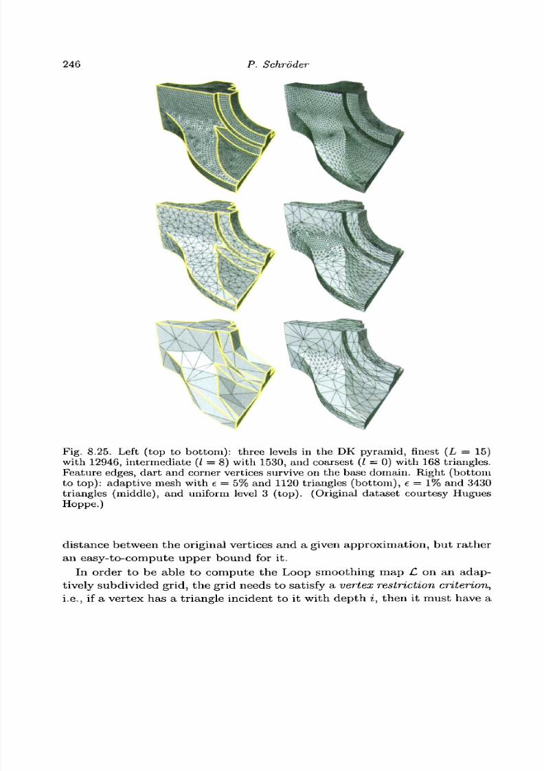
8/3/2019 Multivariate Approximation
http://slidepdf.com/reader/full/multivariate-approximation 256/296
246 P. Schroder
Fig. 8.25. Left (top to bottom): three levels in the DK pyramid, finest (L = 15)with 12946, intermediate (I = 8) with 1530, and coarsest (/ = 0) with 168 triangles.Feature edges, dart and corner vertices survive on the base domain. Plight (bottomto top): adaptive mesh with t = 5% and 1120 triangles (bottom), e = 1% and 3430triangles (middle), and uniform level 3 (top). (Original dataset courtesy HuguesHoppe.)
distance between the original vertices and a given approximation, b ut rather
an easy-to-compute upper bound for it.
In order to be able to compute the Loop smoothing map C on an adap-
tively subdivided grid, the grid needs to satisfy a vertex restriction criterion,
i.e., if a vertex has a triangle incident to it with depth i, then it must have a

8/3/2019 Multivariate Approximation
http://slidepdf.com/reader/full/multivariate-approximation 257/296
Chapter 8 Scalable algorithms in computer graphics 247
Fig. 8.26. Example of a constrained parameterization based on user input. Left:original input mesh (100,000 triangles) with edge tags superimposed in red. Greenlines show some smooth isoparameter lines of our parameterization. The middleshows an adaptive subdivision connectivity remesh. The right one patches cor-responding to the eye regions (right eye was constrained, left eye was not) are
highlighted to indicate the resulting alignment of top level patches with the featurelines. (Dataset courtesy Cyberware.)
complete 1-ring at level i— \ (Zorin et al. (1997)). This restriction may neces-
sitate subdividing some triangles even if they are below the error threshold.
Examples of adaptive remeshing can be seen in Figure 8.15 (lower left) and
Figure 8.25.
Figure 8.26 shows an example of a constrained parameterization and sub-
sequent adaptive remeshing. The original da taset of 100,000 triangles is
shown on the left. The red lines indicate user-supplied feature constrain ts
which may facilitate subsequent animation. The green lines show some rep-
resentative isoparameter lines of our parameterization subject to the red
feature constraints. The middle image shows an adaptive subdivision con-
nectivity remesh with 74698 triangles (e = 0.5%). On the right we have
highlighted a group of patches, two over the right (constrained) eye and
one over the left (unconstrained) eye. This indicates how user-supplied con-
straints force domain patches to align with desired features. Other enforced
patch boundaries are the eyebrows, center of the nose, and middle of lips
(see red lines in left image).
Finally, the example shown in Figure 8.15 starts with an original mesh
(96966 triangles) on the top left and results in an adaptive, subdivision con-
nectivity remesh on the bo ttom left. This remesh was subsequently edited

8/3/2019 Multivariate Approximation
http://slidepdf.com/reader/full/multivariate-approximation 258/296
248 P. Schrdder
in the interactive multiresolution editing system described earlier (bottom
middle).
8.9 Summary
Exploiting multiresolution is now widely considered an important ingredi-
ent in the construction of scalable algorithms for many computer graphics
applications. Such constructions fall into two basic categories, those gener-
alizing classical notions of multiresolution which are intricately connected
with subdivision and w avelets, and those based on mesh simplification. The
former can leverage the considerable mathematical machinery developed for
the classical setting. The latter are still very new and little is known so far
about the construction of smooth functions over the associated mesh hierar-
chies (for first steps in this direction see Daubechies e t al. (1999); Daubechies
et al. (1998); Guskov et al. (1999)).
In this chapter we primarily considered subdivision for surfaces and its
multiresolution extension through the introduction of detail vectors at suc-
cessive levels of subdivision. The resulting representations are very flexible
since they can represent arbitrary 2-manifold surfaces (with boundary). Be-
cause of the hierarchical stru cture many algorithms which are geared towards
delivering interactive performance on small computers are immediately ap-
plicable. For example, adaptive approximation based on local criteria is easy
to include.
Unfortunately many examples of complex geometry, in particular those
coming from 3D scanning sources are not imbued with the particular semi-
regular mesh structure required by subdivision-based algorithms. One way
of addressing this challenge is through remeshing, i.e., resampling of the orig-
inal geometry onto a semi-regular mesh. Once this step is performed all the
advantages of the semi-regular setting apply. We described one such algo-
rithm in detail. It exploits mesh simplification to discover a low-complexity
base complex which can be employed as the domain for the coordinate fun-
ctions describing the original geometry. It is then an easy matter to resample
the original geometry with guaranteed error bounds.
8.10 Outlook
The demands of real applications are often not satisfied by the traditional
constructions arising from th e "mathematical clean room." Examples inc-
lude irregular samples, non-trivial measures, arbitrary topology 2-manifolds,
small com putational budgets, and very large datasets . Because of this we

8/3/2019 Multivariate Approximation
http://slidepdf.com/reader/full/multivariate-approximation 259/296
Chapter 8 Scalable algorithms in computer graphics 249
have witnessed over the last few years increasing attention being devoted to
the generalization of multiresolution from the infinite, regular, tensor prod-
uct setting, to the semi-regular, and, much more recently, to the irregular
setting. In many of these cases algorithms are running ahead of the associ-
ated theory, which often requires completely new tools for analyzing settings
such as irregular samples, or manifolds with non-trivial structure.
The interchange between applications in computer graphics and, more
generally, computer modeling, simulation, and design, and the classical
mathematical treatment of multiresolution has led to significant advances
in both theory and applications and we expect this to continue into the fu-
ture. While processing power keeps increasing there appears no end in sight
for our ability to absorb all available cycles and still be left wanting more.
Similar observations apply to available network bandwidth . Multiresolution
in all its forms will continue to play a central role and the field is wide open
and in need of further, significant advances.
Acknowledgments
The author was supported in part by NSF (ACI-9624957, ACI-9721349,DMS-9874082, DMS-9872890), DOE (W-7405-ENG-48), and the NSF STC
for Com puter Graphics and Scientific Visualization. Other suppo rt was
provided by Alias|wavefront and a Packard Fellowship.
None of this work could have happened without my students and collab-
orators and in particular Wim Sweldens with whom I have been developing
these ideas for the last 5 years.
ReferencesBrown, P.J.C. and Faigle, C.T. (1997). A robust efficient algorithm for point
location in triangulations. Tech. Rep., Cambridge University.Burt, P.J. and Adelson, E.H. (1983). Laplacian pyramid as a compact image code.
IEEE Trans. Commun., 31(4) , 532-540.Catmull, E. and Clark, J. (1978). Recursively generated B-spline surfaces on
arbitrary topological meshes. Comput. Aided Design, 10(6) , 350-355.Certain, A., Popovic, J., DeRose, T., Duchamp, T., Salesin, D. and Stuetzle, W.
(1996). Interactive multiresolution surface viewing. In Computer Graphics
(SIGGRAPH '96 Proceedings), ed. H. Rushmeier, pp. 91-98. Addison Wesley.Cohen, J., Manocha, D. and Olano, M. (1997). Simplifying polygonal models using
successive mappings. In Proceedings IEEE Visualization 91, pp. 395-402.Curless, B. and Levoy, M. (1996). A volumetric method for building complex
models from range images. In Computer Graphics (SIGGRAP H '96Proceedings), ed. H. Rushmeier, pp. 303-312. Addison Wesley.
Daubechies, I., Guskov, I. and Sweldens, W. (1998). Commutation for irregularsubdivision. Tech. Rep., Bell Laboratories, Lucent Technologies.

8/3/2019 Multivariate Approximation
http://slidepdf.com/reader/full/multivariate-approximation 260/296
250 P. Schroder
Daubechies, I., Guskov, I. and Sweldens, W. (1999). Regularity of irregularsubdivision. Const. Approx., 15, 381-426.
DeRose, T., Kass, M. and Truong, T. (1998). Subdivision surfaces in characteranimation. In Com puter Graphics (SIGGRAP H '98 Proceedings), pp. 85-94.
Dobkin, D. and Kirkpatrick, D. (1985). A linear algorithm for determining theseparation of convex polyhedra. J. Algorithms, 6, 381-392.
Doo, D. and Sabin, M. (1978). Analysis of the behaviour of recursive divisionsurfaces near extraordinary points. Comput. Aided Design, 10(6) , 356-360.
Duchamp, T., Certain, A., DeRose, T. and Stuetzle, W. (1997). Hierarchicalcomputation of PL harmonic embeddings. Tech. Rep., University ofWashington.
Dyn, N., Levin, D. and Gregory, J.A. (1990). A butterfly subdivision scheme for
surface interpolation with tension control. ACM Trans. Graphics, 9( 2 ) .160-169.
Eck, M., DeRose, T., Duchamp, T., Hoppe, H., Lounsbery, M. and Stuetzle, W.(1995). Multiresolution analysis of arbitrary meshes. In Computer Graphics(SIGGRAP H '95 Proceedings), ed. R. Cook, pp. 173-182.
Eck, M. and Hoppe, H. (1996). Automatic reconstruction of B-spline surfaces ofarbitrary topological type. In Comp uter Graphics (SIGGRAP H '96Proceedings), H. Rushmeier, pp. 325-334. Addison Wesley.
Finkelstein, A. and Salesin, D.H. (1994). Multiresolution curves. In ComputerGraphics P roceedings, Annual Conference Series, pp. 261-268.
Forsey, D. and Wong, D. (1995). Multiresolution surface reconstruction forhierarchical B-splines. Tech. Rep., University of British Columbia.
Forsey, D.R. and Bartels, R.H. (1988). Hierarchical B-spline refinement.Comp uter Graphics (SIGGRAP H '88 Proceedings), 22(4) , 205-212.
Garland, M. and Heckbert, P.S. (1995). Fast polygonal approximation of terrainsand height fields. Tech. Rep. CMU-CS-95-181, Carnegie Mellon University.
Gortler, S.J. and Cohen, M.F. (1995). Hierarchical and variational geometricmodeling with wavelets. In Proceedings Symposium on Interactive 3DGraphics.
Guibas, L. and Stolfi, J. (1985). Primitives for the manipulation of general
subdivisions and the computation of Voronoi diagrams. ACM Trans.Graphics, 4(2), 74-123.
Guskov, I., Sweldens, W. and Schroder, P. (1999). Multiresolution signalprocessing for meshes. Tech. Rep. PACM TR 99-01, Princeton University,submitted.
Heckbert, P.S. and Garland, M. (1997). Survey of polygonal surface simplificationalgorithms. Tech. Rep., Carnegie Mellon University.
Hoppe, H. (1996). Progressive meshes. In Computer Graphics (SIGGRAP H '96Proceedings), ed. H. Rushmeier, pp. 99-108. Addison Wesley.
Hoppe, H. (1997). View-dependent refinement of progressive meshes. In
Com puter Graphics (SIGGRAP H '97 Proceedings), pp. 189-198.Hoppe, H., DeRose, T., Duchamp, T., Halstead, M., Jin, H., McDonald, J.,
Schweitzer, J. and Stuetzle, W. (1994). Piecewise smooth surfacereconstruction. In Com puter Graphics (SIGGRAP H '94 Proceedings), pp.295-302.
Kirkpatrick, D. (1983). Optimal search in planar subdivisions. SIAM J. Comput.,12, 28-35.
Klein, A., Certain, A., DeRose, T., Duchamp, T. and Stuetzle, W. (1997).

8/3/2019 Multivariate Approximation
http://slidepdf.com/reader/full/multivariate-approximation 261/296
Chapter 8 Scalable algorithms in computer graphics 251
Vertex-based Delaunay triangulation of meshes of arbitrary topological type.Tech. Rep., University of Washington.
Kobbelt, L. (1996a). Interpolatory subdivision on open quadrilateral nets witharbitrary topology. In Proceedings of Eurographics '96, pp. 409-420.Computer Graphics Forum.
Kobbelt, L. (1996b). A variational approach to subdivision. Comput. AidedGeom. Des., 13, 743-761.
Krishnamurthy, V. and Levoy, M. (1996). Fitting smooth surfaces to densepolygon meshes. In Computer Graphics (SIGGRAP H '96 Proceedings), ed .H. Rushmeier, pp. 313-324. Addison Wesley.
Levin, A. (1999). Combined subdivision schemes for the design of surfacessatisfying boundary conditions. Comput. Aided Geom,. Des., to appear.
Loop, C. (1987). Smooth subdivision surfaces based on triangles. Master's thesis,University of Utah, Department of Mathematics.Lounsbery, M. (1994). Multiresolution analysis for surfaces of arbitrary topological
type. PhD thesis, Department of Computer Science, University ofWashington.
Lounsbery, M., DeRose, T. and Warren, J. (1997). Multiresolution analysis forsurfaces of arbitrary topological type. ACM Trans. Graphics, 16(1) , 34-73.
Peters, J. and Reif, U. (1997). The simplest subdivision scheme for smoothingpolyhedra. A CM Trans. Graphics, 16(4) .
Prautzsch, H. and Umlauf, G. (1998). Improved triangular subdivision schemes.
In Proceedings of the CGI '98.Schroder, P ., and Sweldens, W. (1995). Spherical wavelets: Efficientlyrepresenting functions on the sphere. In Computer Graphics (SIGGRAPH'95 Proceedings), ed. R. Cook.
Schweitzer, J.E. (1996). Analysis and application of subdivision surfaces. PhDthesis, University of Washington, 1996.
Stam, J. (1998). Exact evaluation of Catmull-Clark subdivision surfaces atarbitrary parameter values. In Com puter Graphics (SIGGRAP H '98Proceedings), pp. 395-404.
Sweldens, W. (1996). The lifting scheme: A custom-design construction ofbiorthogonal wavelets. Appl. Comput. Harmon. Anal., 3(2), 186-200.
Sweldens, W. and Schroder, P. (1996). Building your own wavelets at home. InWavelets in Computer Graphics, pp. 15-87. ACM SIGGRAPH Course Notes.
Taubin, G. (1995). A signal processing approach to fair surface design. InCom puter Graphics (SIGGRAP H '95 Proceedings), ed. R. Cook, pp. 351-358.Annual Conference Series.
Xia, J.C. and Varshney, A. (1996). Dynamic view-dependent simplification forpolygonal models. In Proc. 'Visualization 96, pp. 327-334.
Zorin, D. (1997). Stationary subdivision and multiresolution surfacerepresentations. PhD thesis, California Institute of Technology.
Zorin, D., Schroder, P. and Sweldens, W. (1996). Interpolating subdivision formeshes with arbitrary topology. In Computer Graphics (SIGGRAP H '96Proceedings), ed. H. Rushmeier, pp. 189-192. Addison Wesley.
Zorin, D., Schroder, P. and Sweldens, W. (1997). Interactive multiresolution meshediting. In Com puter Graphics (SIGGRAP H '97 Proceedings), pp. 259-268.

8/3/2019 Multivariate Approximation
http://slidepdf.com/reader/full/multivariate-approximation 262/296
9
Mathematical methods in reverse engineering
J. HOSCHEK
A b s t r a c t
In many areas of industrial applications it is desirable to create a computer
model of existing objects for which no such model is available. This process
is called reverse engineering. In this chapter we will be concerned with
reverse engineering of the shape of surfaces of objects. We will develop
computer models which provide gains in efficiency of design, modification
and m anufacture. Reverse engineering typically sta rts with digitising anexisting object. These discrete da ta m ust then be converted into smooth
surface models.
9.1 Introduction
In the computer-assisted manufacturing process there often remain objectswhich are not originally described in a CAD-system. Th e reasons for this
are:• modifications (grinding down or pu ttin g on of material) of existing par ts,
which are required in order to improve the quality of the product;
• copying a part, when no original drawings are available;
• real-scale clay or wood models which are needed as stylists and m anage-
ment often prefer real 3D objects for evaluation, rather than projections
of objects on 2D screens at reduced scale.
These physical objects are measured by mechanical digitising machinesor laser scanners or Moire-based optical sensors. The resulting dataset may
be partially ordered (digitising machines) or unorganised (laser scanners),
and has to be transformed into smooth surfaces. As is mentioned in Varady
et al. (1997) the main purpose of reverse engineering is to convert discrete
datasets into piecewise smooth, continuous models.
252

8/3/2019 Multivariate Approximation
http://slidepdf.com/reader/full/multivariate-approximation 263/296
Chapter 9 Reverse engineering 253
We will not discuss technical aspects of rapid prototyping and of data
acquisition (Varady et al. (1997)). Rather, we assume that the data acquir-
ing is finished and we have a suitable organisation of da ta : regular da ta
with boundary curves, scattered data with boundary curves or unorganised
clouds of points. We will be concerned w ith the two most critical par ts of
reverse engineering: segmentation and surface fitting.
We mainly consider approximations by free-form surfaces with rectan-
gular structu re of boundary curves. The most important m ethods in this
field are the feature-line-oriented and the region-growing approach . The
natural division lines (feature lines) of a physical object are determined by
computer-vision techniques (especially sharp edges), by numerical or geo-
metric criteria or by the experience of the user. Each feature line L of
the physical object corresponds to a polygonal or to a piecewise polynomial
curve. The set of all curves may be deno ted by C = C(L). The user has
to subdivide manually or with the help of suitable algorithms, the set C(L)
into a finite number of (rectangular) regions Ri- Afterwards for each region
a surface S(Ri) is generated by least squares fitting with respect to a pre-
scribed error tolerance and satisfying the continuity requirements imposed
by the user.
Region-growing methods start at a seed point or a (small) seed region
(Sapidis and Besl (1995)). The seed region R is approximated in the least
squares sense by a polynomial surface 5, followed by an iterative process,
where first R is growing iteratively to include all points in the neighbour-
hood of the seed region which hold the prescribed error tolerance between
the approximation surface S and the given points. Thu s, algorithms are
developed for maximising the amount of data represented by a polynomial
surface which guarantees that the distance error between the given points
and the surface is smaller than a prescribed tolerance.
These two strategies are called bottom-up methods (Varady et al. (1997)).
On the other hand top-down methods are developed startin g w ith the premise
that all points belong to a single surface. If a prescribed error tolerance is
exceeded by a single approximating surface the points in the critical areas
are subdivided by the user into a suitable number of new sets, which are
further approximated. Although users would like to have a fully automatic
system which can detect and classify feature lines without any user inter-
action, with the present state of the art all CAD-systems need more or less
a priori information or assumptions on the object, connected with manual
interac tions. Fig. 9.1 shows a real example: a datase t of 400,000 points from
a joystick and a manual segmentation in 48 B-spline patches. The engineer
needed 5 hours whilst using the CAD-system SURFACER from Imageware,
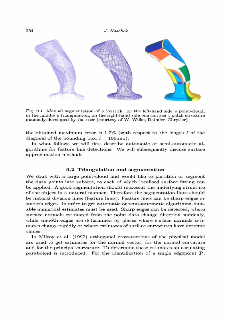
8/3/2019 Multivariate Approximation
http://slidepdf.com/reader/full/multivariate-approximation 264/296
254 J. Hoschek
Fig. 9.1. Manual segmentation of a joystick: on the left-hand side a point-cloud,in the middle a triangulation, on the right-hand side one can see a patch structuremanually developed by the user (courtesy of W. Wilke, Daimler-Chrysler)
the obtained maximum error is 1.7% (with respect to the length I of thediagonal of the bounding box, I = 190mm).
In what follows we will first describe automatic or semi-automatic al-
gorithm s for feature line detections. We will subsequently discuss surface
approximation methods.
9.2 Triangulation and segmentation
We start with a large point-cloud and would like to partition or segmentthe data points into subsets, to each of which localised surface fitting can
be applied. A good segmentation should represent the underlying structure
of the object in a natural manner. Therefore the segmentation lines should
be natural division lines (feature lines). Feature lines can be sharp edges or
smooth edges. In order to get autom atic or semi-autom atic algorithms, suit-
able numerical estimates must be used. Sharp edges can be detected, where
surface normals estimated from the point data change direction suddenly,
while smooth edges are determined by places where surface normals esti-mates change rapidly or where estimates of surface curvatures have extreme
values.
In Milroy et al. (1997) orthogonal cross-sections of the physical model
are used to get estimates for the normal vector, for the normal curvature
and for the principal curvature. To determine these estimates an osculating
paraboloid is introduced. For the identification of a single edgepoint P ,

8/3/2019 Multivariate Approximation
http://slidepdf.com/reader/full/multivariate-approximation 265/296
Chapter 9 Reverse engineering 255
the pr incipal curvature di rect ions are used. The surface curvature on ei ther
side of the point P in a princip al direction m i is est im ate d by n eighb ourin g
osculat ing paraboloids . If the pr incipal curvature K\ i s a local maximum,
th e poin t is flagged as an edge poin t. Sim ilarly th e princip al direc tion rri2
is used to decide wh ether the pr incipal curvatur e «2 is a m axim um . T he
set of edge points is connected by energy-minimising snake splines (Kass et
al. (1987)).
1 i
Fig. 9.2. Cloud of 95,436 disorganized points digitised from a mechanical model(courtesy of W. Wilke, Daimler-Chrysler)
In Lukacs and Andor (1998), a differential geometric approach is devel-
oped based on triangulated point data with normal vector and curvature
estimations at these points. On the triangulation a set of points is de-
termined so that the principal curvature is stationary (i.e., the principal
curvature has an extremal value) in the corresponding principal direction.
The curves connecting such stationary points are called ridges (local posi-
tive maximum of principal curvature) or ravines (local negative minimum of

8/3/2019 Multivariate Approximation
http://slidepdf.com/reader/full/multivariate-approximation 266/296
256 J. Hoschek
principal curvature). Ridges and ravines are natural dividing lines between
regions of monotone principal curvature.
We will now describe in detail a fast bottom-up algorithm which deter-
mines feature lines using an edge-based technique combined with region-
based properties (Hoschek et al. (1998), Wilke (2000)). As an example we
will use a cloud of disorganised points scattered on the surface of a body
having some holes (see Fig. 9.2). This cloud contains 95,436 points and was
generated by an optical sensor with 2-range images.
To determine the feature lines, we will triangulate the given cloud of
points. In the past many algorithms were developed for 3D-triangulations
of disorganised data. Well-known examples are: 3D-Delaunay triangulations
or marching-cube based algorithms.
For surface reconstruction with a large da tase t (more tha n 100,000 points) ,
these a lgorithm s are mostly too slow and often lead only to the convex hull of
the given dataset. The fast algorithm using a multistep procedure developed
in Wilke (2000) is as follows.
• The dataset is first subdivided into regular solids (voxels) of a basis size
chosen by the user. The points in a voxel are then projected on its leastsquares plane. If this projection is not unique, the voxels are refined. W ith
the help of an octree data structure the topology of the object can be re-
constructed, since the octree data structure gives implicit neighbourhood
information between the voxels. We remark th at the given da ta cloud
may be related to an open or a closed surface.
• In each least squares plane the points are triangu lated by a planar Delau-
nay triangulation and then lifted to a 3D-triangulation of the points in
the voxel (see Fig. 9.3).
• Th e edges of each voxel triangulation are now connected with neighbour-
ing voxels using a stitching algorithm introduced in Shewchuck (1995).
Due to measurement errors some gaps may remain. These must be closed
interactively.
On a Pentium II 266 MHz this multistep algorithm requires four seconds
for the planar Delaunay triangulations of 100,000 points (Fig. 9.3), and five
seconds for closing the gaps.For point-clouds with unknown topology a region growing methodf should
be used as follows:
• split the point-cloud into voxels, and compute the voxel centre points;
t This algorithm may fail for nonsensical data like a flat triangulation connected with highcurvature values. In that case no starting point can be found automatically.
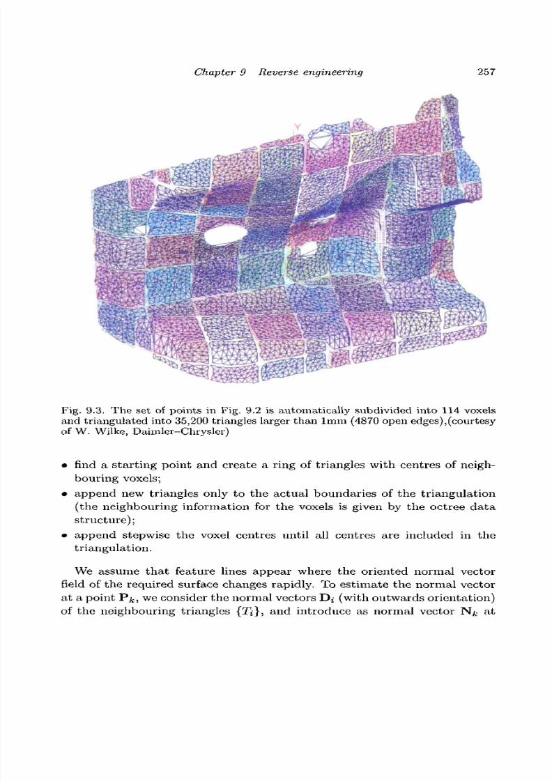
8/3/2019 Multivariate Approximation
http://slidepdf.com/reader/full/multivariate-approximation 267/296
Chapter 9 Reverse engineering 257
Fig. 9.3. The set of points in Fig. 9.2 is automatically subdivided into 114 voxelsand triangulated into 35,200 triangles larger than lmm (4870 open edges),(courtesy
of W. Wilke, Daimler-Chrysler)
• find a start ing point and c reate a ring of triangles with centres of neigh-
bouring voxels;
• append new triangles only to the actua l boundaries of the triangulation
(the neighbouring information for the voxels is given by the octree data
structure);
• append stepwise the voxel centres until all centres are included in thetriangulation.
We assume that feature lines appear where the oriented normal vector
field of the required surface changes rapidly. To estimate the normal vector
at a point P ^ , we consider the normal vectors Dj (with outwards orientation)
of the neighbouring triangles {Tj}, and introduce as normal vector Nj- at
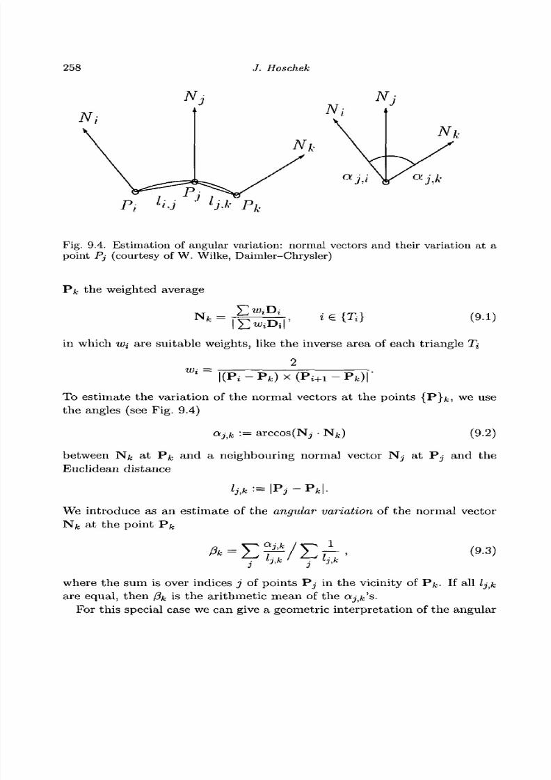
8/3/2019 Multivariate Approximation
http://slidepdf.com/reader/full/multivariate-approximation 268/296
258 J. Hoschek
Fig. 9.4. Estimation of angular variation: normal vectors and their variation at apoint Pj (courtesy of W. Wilke, Daimler-Chrysler)
'fc the weighted average
Nfc = i € (9.1)
in which u>i are suitable weights, like the inverse area of each triangle Ti
2Wi =
To estimate the variation of the normal vectors at the points {P}fc, we use
the angles (see Fig. 9.4)
tk •= a r ccos ( Nj (9.2)
between N& at P^ and a neighbouring normal vector N j at Pj and the
Euclidean distance
ljik:=\Pj-Pk\.
We introduce as an estimate of the angular variation of the normal vector
Nfc at the point Pfc
(9.3)2s i • v.
where the sum is over indices j of points Pj in the vicinity of Pfc. If all lj tk
are equal, then /3fc is the arith metic mean of the ctj,k's.
For this special case we can give a geometric interpretation of the angular
8/3/2019 Multivariate Approximation
http://slidepdf.com/reader/full/multivariate-approximation 269/296
Chapter 9 Reverse engineering 259
variat ion. Consider the normal curva tu re nn at the point Pfc. By the well-
known Euler formula (Do Carmo (1976)) the normal curvature equals
Kn = Ki cos tp + K2 sin ip , (9-4)
with Ki as principal curvatures and <p as the angle formed with the principal
curvature direction corresponding to Kj. Equation (9.4) leads to an integral
representation of the mean curvature H^ at the point P&
1 f2n
1 f2n
7T- / nn(Pk)dip = — / (KI(Pk)cos
2
ip + K2{Pk)sin
2
'<p)dtpLft J0 tft Jo
If we discretize the continuous function nn in n^ directions y>j (i =
1, ...,rifc) with normal curvatures K3
n we obtain
nkj-l
We can estimate the normal curvatures Kn by the angle otjk between the
normal vector N^ at P^ and the normal vector Nj at the points Pj of the
neighbourhood of P&. Thus the last equation can be written as
1 v—-v
The angular variations can be used to recognise flat regions in the senseof a region-based technique. Regions with very small or no changes of j3
could be expected to be flat. The corresponding triangles are cancelled and
the arising gaps are suitably closed. Moreover, this step reduces the data
volume.
Before starting the segmentation procedure it may be necessary to smooth
out parts of the cloud of points in order to reduce the effect of measurement
errors during the laser-scanning process. To decide whether a data point
Po of the cloud should be corrected, we consider the least squares planeSo determined by the points {Pj} (j = l,...,n) in the vicinity of Po- The
plane eo may have normal vector N passing through the centre of gravity S of
{Pj}. To avoid rounding of sharp edges we only smooth those points whose
angular variation (5 of their normal vector is less than a given threshold
angle a. On the other hand points must be excluded where large changes
of curvature can be expected. Therefore a maximal deviation dmax of the

8/3/2019 Multivariate Approximation
http://slidepdf.com/reader/full/multivariate-approximation 270/296
260 J. Hoschek
Fig. 9.5. Changes of angular variation are the loci of the expected feature lines.They separate planar and nonplanar parts of the object (courtesy of W. Wilke,Daimler-Chrysler)
points i s prescr ibed, which wi l l be based on the noise of the measurement
(e.g. dm a x = 0.1mm). The smoothed point wi l l assume the posi t ion
P o = P o - Nd with d = min(N • (P o - S), d m a x) .
Feature lines can be expected in regions in which the angular variation
changes rapidly. To avoid indication errors, the d ata are smoothed with
the help of an erosion operator! (Haberacker (1991)) before feature linedetection . In Sarkar and Menq (1991) a Laplace operator was used bu t
from our experience the erosion operator leads to much better results.
To indicate the changes of the angular variation, we use a colour map for
the angular variation p. For each triangle the values /% at the various colours
f Erosion in a point Po is defined by min(Ko, Mneighbouring points {Pj} of Po.
, • • • «fc) with Kj as curvature values of the
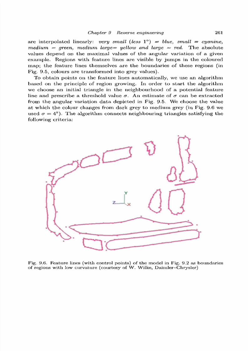
8/3/2019 Multivariate Approximation
http://slidepdf.com/reader/full/multivariate-approximation 271/296
Chapter 9 Reverse engineering 261
are interpolated linearly: very small (less 1°) = blue, small = cyanine,
medium = green, medium large= yellow and large = red. The absolute
values depend on the maximal values of the angular variation of a given
exam ple. Regions with feature lines are visible by jum ps in the coloured
map; the feature lines themselves are the boundaries of these regions (in
Fig. 9.5, colours are transformed into grey values).
To obtain points on the feature lines automatically, we use an algorithm
based on the principle of region growing. In order to sta rt the algorithm
we choose an initial triangle in the neighbourhood of a potential feature
line and prescribe a threshold value a. An estimate of a can be extracted
from the angular variation data depicted in Fig. 9.5. We choose the value
at which the colour changes from dark grey to medium grey (in Fig. 9.6 we
used a = 4°). The algorithm connects neighbouring triangles satisfying the
following criteria:
Fig. 9.6. Feature lines (with control points) of the model in Fig. 9.2 as boundariesof regions with low curvature (courtesy of W. Wilke, Daimler-Chrysler)
8/3/2019 Multivariate Approximation
http://slidepdf.com/reader/full/multivariate-approximation 272/296
262 J. Hoschek
• each triangle is inspected only once.
• the minimal angular variations at the vertices of the neighbouring trian-gles are less than a. The triangles which fulfil this criteria are also the
candidates for the initial triangles of the first step in the region growing
process.
• the changes between minimal angular variation at the vertices of one trian-
gle and the maximal angular variation at the vertices of the neighbouring
triangles are less than a.
As a result we obtain triangulated feature regions and polygonal lines asthe boundaries. These polygonal lines are approximated by cubic B-spline
curves with the use of energy constraints (minimal length of the control
polygon), leading to the required B-spline representation of the feature lines
(see Fig. 9.6).
After determining feature lines we have various alternatives on how to
proceed.
• Detect quadrilateral faces or loops in the network of feature lines or in-
troduce manually (or automatically) connecting curves to get a quadri-
lateral network covering the whole cloud of points. Afterwards all these
quadrilateral regions have to be approximated by B-spline surfaces with
a prescribed error tolerance and continuity requirements imposed by the
user (bottom-up strategies);
• Approximate the whole cloud of points with a single overall B-spline sur-
face using free boundaries and energy constraints. If the given error tol-erance is exceeded by the single B-spline surface in some parts of the
surface, improve the quality of approximation in these bad regions with
the help of the local feature lines in the vicinity of the bad region. These
local feature lines can be boundary curves or trimming curves of a new
local approximation surface approximating the bad regions of the single
overall approximation surface with respect to the given error tolerance.
Thus we get a patchwork of approximation surfaces containing the over-
all B-spline approximation surface and the local B-spline approximationsurfaces improving the approximation quality of the bad regions of the
overall approximation. At the trimming or boundary curves of the new
surface patches continuity requirements must be fulfilled (top-down strat-
egy). Hoschek et al. (1998) call this a geometric concept of reverse engi-
neering (see Fig. 9.7).

8/3/2019 Multivariate Approximation
http://slidepdf.com/reader/full/multivariate-approximation 273/296
Chapter 9 Reverse engineering 263
cloud of points
overall B-spline surface triangulation
boundaries as trimmingcurves
estimate normals, curvature
regions with feature lines
elsefeature lines
improving B-spline surfacelocally
Fig. 9.7. Geometric concept of reverse engineering
9.3 Approximation
Following the first alternative (bottom-up ) we assume tha t the boundaries of
the B-spline surface patches (faces) have a rectangular struc ture. In this case
we first approxim ate the four bou ndary curves by four (open) B-spline curves
of given order k and a given knot-sequence by the least squares method. We
start with a suitable initial parametrisation (chordal, centripetal) (Hoschek
and Lasser (1993)) and improve the parametrisation by local reparametri-
sation (Hoschek and Lasser (1993)) or global reparametrisation (Speer et
al . (1998)).
The four boundary curves determine a reference surface for parametri-
sation of the interior po ints P i (z = l,...,r) of the face. As reference
surface a bilinear Coons patch or tensor-product B-spline surface C with
a small number of knots can be chosen. Now we project (perpendicular
to C) the interior points P , of the given cloud on C. The closest point
Pi of C determines an initial guess of parameter values ( M , , ^ ) of Pj in
the corresponding parameter domain. With this initial parametrisation of
P , the given set of points is approximated by one tensor-product B-spline
surface with fixed order k in the parametric representation (Farin (1996),

8/3/2019 Multivariate Approximation
http://slidepdf.com/reader/full/multivariate-approximation 274/296
264 J. Hoschek
Hoschek and Lasser (1993))
n mX{u, v) = J2 Yl
di '
Nik(n)Nik(v), (9.5)
j=o /=o
where the parameter values are defined with respect to suitably chosen knot
sequences U, V, while the d y are the unknown control points .
The objective function of the approximation problem is the reduction of
the dis tances between the given points P j and the required surface. T hu s
we would l ike to minimise
( ) (9-
6)
The minimisation of (9.6) is obtained by well-known least squares tech-
niques , in which the boundary control points do; ,d n / , d j o , d j m are known
from the approximat ion of the boundary curves .
For the second alternative (overall approximation) the use of the usual
least squ ares surface appro xim atio n is l imited in several way s. To o bta in
a un ique approximat ion sur face the Schoenberg-Whi tney condi t ions mus t
be satisfied. This requires well-distr ibuted point-sets without holes. But an
overal l approximat ion must take into account holes in the dataset and non-
rectan gular d om ains . Therefore , we should use an appro xim at ion w i th free
bou nda r ies . Free bou ndar ies of an approx im at ion surface can be obta ined
as the boundaries of a suitable rectangle in a least squares plane of the given
set of points, where the boundaries of the given set of points l ie total ly in
the interior of the rectangle. The planar rectangle is an init ial guess of the
required appro xim at ion surface. If th e point -set is mo re com plicated, m ore
sophis t icated surface types must be chosen. The only condi t ion which must
be fulfilled by the surface initially guessed is that the perpendicular projec-
tion of the given points onto the surface be bijective. This initial guess of an
approximat ion surface wi l l be deformed towards the given point -set dur ing
the approximat ion process .
To fulfi l l the Schoenberg-Whitney condit ion for the holes and the domain
without points between the given boundar ies of the dataset and the rect -
angular free boundaries of the approximation surface, we introduce a new
objective combined with a fairness measure Qfa;r, and we minimise a new
objective functional
r . (9.7)
Here A is a penalty factor controlling the influence of the fairness functional.

8/3/2019 Multivariate Approximation
http://slidepdf.com/reader/full/multivariate-approximation 275/296
Chapter 9 Reverse engineering 265
It can be determined automatically during an iterative algorithm (Dietz
(1996)). Using this new objective functional we can handle point-sets of
varying density, point-sets with holes and with nonrectangular boundary
curves, and point-sets with measurement errors. A number of suggestions
for such fairness functionals can be found in Bloor et al. (1995), Greiner
(1994), Moreton and Sequin (1992), Rando and Roulier (1991). Applica-
tions are described in Dietz (1996), Hadenfeld (1995), Hagen and Schulze
(1987), Sinha and Schunck (1992), Welch and Witkin (1992). Many of these
functionals are related to physical energies. For example, / («j + K |) dS is
the bending energy of a thin plate with small deflections (with KI,K,2 prin-
cipal curvatures). But this energy, like many others, depends highly non-
linearly on the unknown control points. If a fairness functional is quadratic
in the unknowns, the resulting system of equations is linear. The following
functionals are some examples of simplified measures for the area, bending
energy and change of curvature of a surface X. They are all quadratic in the
control points,
X2
u + X2
v)dudv, (9.8)
Q 2 = IIX2UU + 2X
2UV + X
2
vvdu dv, (9.9)
Q 3 = f f (Xuuu + Xuvv)2
+ {Xuuv + Xvvv)2
du dv. (9.10)
These quan tities may be combined in a convex manner to define a fairness
functional3 3
Qfair = ^2o:pQp , With ^ ap = 1 .P = i P = i
The factors ap control the influence of the individual functionals and hence
the shape of the resulting surface. These so-called design factors ap are to
be determined by the user.
A necessary condition for the functional Q to be minimal is
This leads to the linear system
A d = b with A = A d i s t + AA fair and A fa i r = ^ a p A p . (9.11)
v
Here Adist is the matrix of the usual normal equations and b is the cor-
responding right-hand side. The vector d contains the unknown control
8/3/2019 Multivariate Approximation
http://slidepdf.com/reader/full/multivariate-approximation 276/296
266 J. Hoschek
points. Equation (9.11) is actually a system of equations with three right-
hand sides (one for each coordinate). The matrices A p correspond to the
energies Q p and do not depend on the point param etrisation. The m atrix
Afa[r can therefore be precalculated. Only the matrix AdjSt changes after
the reparametrisation described below.
By using B-splines, the matrices A p , Afa;r are symmetric, positive semi-
definite and banded with the same bandwidth as the matrix AdiSt for the
usual least squares fit. The elements of A p are determined by integrals
over produc ts of B-spline basis functions. These integrals can be calculated
exactly as the integrals are piecewise polynomials (Dietz (1996)). Subject to
some weak conditions on the dataset, the approximation surface is uniquely
determined (Dietz (1996)).
After solving (9.11) we update the initial parametrisation to improve
the quality of the approximation surface. Both steps, approximation and
reparametrisation, are repeated in a loop until an end condition is satisfied
(e.g., the approxim ation error is sufficiently small). For reparam etrisa tion
we can use a local approach (Hoschek and Lasser (1993), Hoschek and Dietz
(1996)). For each point Pj the corresponding parameter values (iH,Vi) are
replaced by the parameter values (M, = Ui + AM, x>i = VJ + Av) of the closest
point to P j on the surface X . This is done by Newton's method which is
locally convergent of order 2. The correction terms are given by
(Au\ = f X2
U + (X-P)X U U XUXV+(X-P)XUV\ ~V(X-P)XU\\Av) \XUXV+(X-P)XUV X2
V+(X-P)XVV ) {(X-P)XJ-[J- '
In general, we obtain sufficient accuracy after 1 to 3 iterations beginning
with P = Pi. The reparametrisation together with the approximation, in-
cluding the fairing functional, is very robust and the approximation surfaces
are both smooth and stiff (Dietz (1996)).
Our overall approximation may be insufficient on domains with a rapid
change of curvatu re. An add itional local improvement is therefore intro-
duced. As a local energy constraint we again use the thin-plate energy
Qfair = J j A(U, V) (X2
UU + 2X2
UV + X2
m) dudv
weighted by the real-valued B-spline function
\{u, v) = ^2J2 WijNiriujNjsiv) > 0 (wij e R) .
This functional surface A allows us to locally control the influence of the
energy term. In flat regions A can be chosen large with a strong smoothing
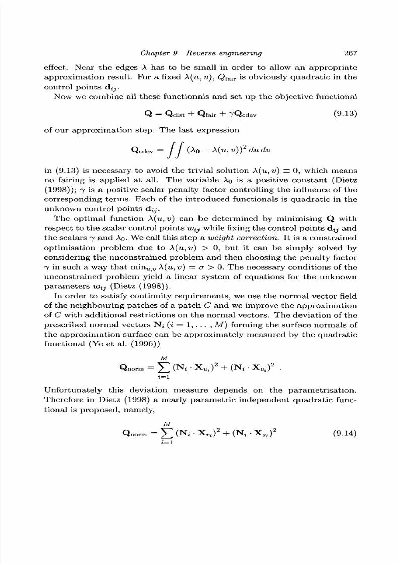
8/3/2019 Multivariate Approximation
http://slidepdf.com/reader/full/multivariate-approximation 277/296
Chapter 9 Reverse engineering 267
effect. Near the edges A has to be small in order to allow an app rop riate
approximation result. For a fixed \(u, v), Qfair is obviously quadratic in the
control points dy.
Now we combine all these functionals and se t up the objective functional
Q = Qdist + Qfair + 7Qcdev (9-13)
of our approximation step. The last expression
Qcdev = / / (Ao - \(u,v))2
dudv
in (9.13) is necessary to avoid the trivial solution \(u,v) = 0, which means
no fairing is applied a t all. The variable Ao is a positive constant (Dietz
(1998)); 7 is a positive scalar penalty factor controlling the influence of the
corresponding terms. Each of the introduced functionals is quadratic in the
unknown control points dy.
The optimal function A(M, V) can be determined by minimising Q with
respect to the scalar control points wy- while fixing the control poin ts d y and
the scalars 7 and Ao. We call this step a weight correction. It is a constrainedoptimisation problem due to \(u, v) > 0, but it can be simply solved by
considering the unconstrained problem and then choosing the penalty factor
7 in such a way that minUjl) \(u, v) = a > 0. The necessary conditions of the
unconstrained problem yield a linear system of equations for the unknown
parameters Wy (Dietz (1998)).
In order to satisfy continu ity requ irements, we use the normal vector field
of the neighbouring patches of a patch C and we improve the approximation
of C with additional restrictions on the normal vectors. The deviation of the
prescribed normal vectors Nj (i = 1,... , M) forming the surface normals of
the approximation surface can be approximately measured by the quadratic
functional (Ye et al. (1996))
M
\ ^ /"i\r "v \^ _i_ /T\r Y \^n o r m — / \*-*i ' -t^-iti) > \^*i ' -**-V()
Unfortunately this deviation measure depends on the parametrisation.Therefore in Dietz (1998) a nearly parametric independent quadratic func-
tional is proposed, namely,
M
Qnorm = £( !*<• X, , )2
+ (N< • X s ; )2
(9.14)i = l
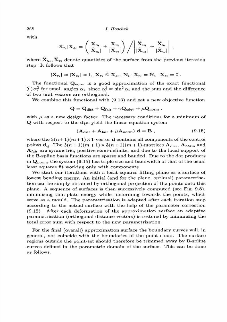
8/3/2019 Multivariate Approximation
http://slidepdf.com/reader/full/multivariate-approximation 278/296

8/3/2019 Multivariate Approximation
http://slidepdf.com/reader/full/multivariate-approximation 279/296
Chap ter 9 Reverse engineering 269
Fig. 9.8. 3234 data points with surfaces after 1, 7, 10, 14, 18 iteration steps (cour-tesy of U. Dietz)
The boundary points {R}i are projected perpendicularly onto the surface
and then for each projected point the preimage (ui,Vi) in the parametric
domain is calculated.
These points (iii,Vi) are approximated by a 2D B-spline curve (Hoschek
and Schneider (1992))
C(t) = ( « ( (9.16)
using least squares techniques and parameter correction. The error distance
is measured in R3
whereas the approximation works in the parametric do-
main. The final trimming curve is obtained by inserting C(t) into the surface

8/3/2019 Multivariate Approximation
http://slidepdf.com/reader/full/multivariate-approximation 280/296
270 J. Hoschek
Fig. 9.9. An overall approximation of the cloud of points in Fig. 9.2 with trimmedboundary curves as natural boundaries of the given cloud of points and blendingpatches determined by feature lines (courtesy of W. Wilke, Daimler-Chrysler)
representation of X, i.e., ~X.(u(t),v(t)). In a similar way holes can be per-
formed in the interior of the surface if the point-cloud requires it.
Fig. 9.9 contains an overall approximation of the given cloud of points of
Fig. 9.2 with trim ming curves as natural boundaries of the given set of points
with a maximal approximation error of 1.1%. To improve the approximation
surface, six trimmed (blending) surface patches (bicubic B-spline surfaces)
are constructed on the basis of the corresponding feature lines (see Fig. 9.6)
for the domains with large deviations from the given set of points. Thus, the
maximal error is reduced to 0.6% (with respect to the length of the diagonal
of the bounding box, 228mm).
To demonstrate the effectiveness of the developed methods we again con-
sider the joystick from Fig. 9.1. Because of the topology of the object,
the cloud of points was manually split into three parts to get appropriate
approximation surfaces by an overall approximation. For bo th sides of the
object, 30 x 30 bicubic B-spline surfaces were used, while the top was app-
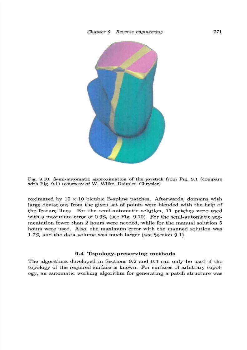
8/3/2019 Multivariate Approximation
http://slidepdf.com/reader/full/multivariate-approximation 281/296
Chap ter 9 Reverse engineering 271
Fig. 9.10. Semi-automatic approximation of the joystick from Fig. 9.1 (comparewith Fig. 9.1) (courtesy of W. Wilke, Daimler-Chrysler)
roximated by 10 x 10 bicubic B-spline patches. Afterwards, domains with
large deviations from the given set of points were blended with the help of
the feature lines. For the semi-autom atic solution, 11 patches were used
with a maximum error of 0.9% (see Fig. 9.10). For the semi-automatic seg-
mentation fewer than 2 hours were needed, while for the manual solution 5
hours were used. Also, the m aximum error with the manned solution was
1.7% and the data volume was much larger (see Section 9.1).
9.4 Topology-preserving methods
The algorithms developed in Sections 9.2 and 9.3 can only be used if the
topology of the required surface is known. For surfaces of arbitrary topol-
ogy, an automatic working algorithm for generating a patch structure was

8/3/2019 Multivariate Approximation
http://slidepdf.com/reader/full/multivariate-approximation 282/296
272 J. Hoschek
proposed in Eck and Hoppe (1996). One starts with a basic triangulation
Mo of the given points with respect to a given error tolerance 6, by using
the triangulation algorithm introduced by Hoppe et al. (1992). The given
points are projected onto the corresponding faces of the triangulation in
order to obtain an initial parametrisation and a parametric domain of the
same topology as the required surface. This triangulation MQ consists of
many faces. These faces are reparametrised in order to get a simple base
complex K& and a continuous map PA:
-KA —* M)- In order to obtain a
low metric torsion PA is constructed with the help of harmonic maps (Eck
et al. (1995)). By merging pairs of triangles of K&, a new base complex
K[j is constructed, the faces of which consist of quadrilate rals. One s ta rts
with a user-chosen seed point in order to automatically generate a quadrilat-
eral patch structure. In addition the parametrisation of K& is transformed
to KQ. Over KQ a control mesh M x is constructed using Peters' scheme
(Peters (1995)), which collectively defines an initial control network of G1-
continuous tensor product B-spline patches of low degree. This network is
improved upon by least squares with energy constraints (see Section 9.3) in
order to obtain surface patches which are as close as possible to the corre-
sponding given points. If these approximating patches differ more than the
user's specified distance error e, KQ will be subdivided into smaller quadri-
lateral surfaces. This method leads to a refined domain complex and a new
B-spline control mesh which covers the given set of points completely and
also attains the required error tolerance.
In Guo (1997) a similar approach was developed. As an initial guess of the
required surface a simplicial surface M (a polygonal mesh with triangular
faces) capturing the topology structure of the set of points is constructedby interactive use of a-shapes (Edelsbrunner and Miicke (1994)). Based on
this structure a curvature continuous surface M is built using least square
methods and generalised B-splines (Loop and DeRose (1990)).
These approaches are very useful for visualisation of objects with unknown
topology. For practical applications in mechanical engineering these tech-
niques have one disadvantage. The triangulation depends on the choice of
some parameters and cannot divide a surface into series of natural division
lines like sharp edges and feature lines.
9.5 Convexity-preserving methods
In this section we present methods for fitting convex (or concave) tensor-
produ ct spline surfaces. The re are two types of methods available in the
literatu re. These are the use of Powell-Sabin spline functions over special
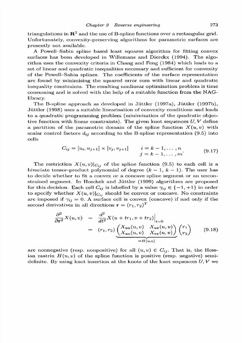
8/3/2019 Multivariate Approximation
http://slidepdf.com/reader/full/multivariate-approximation 283/296
Chapter 9 Reverse engineering 273
triangulations in R2
and the use of B-spline functions over a rectangular grid.
Unfortunately, convexity-preserving algorithms for parametric surfaces are
presently not available.
A Powell-Sabin spline based least squares algorithm for fitting convex
surfaces has been developed in Willemans and Dierckx (1994). The algo-
rithm uses the convexity criteria in Chang and Feng (1984) which leads to a
set of linear and quadratic inequalities necessary and sufficient for convexity
of the Powell-Sabin splines. The coefficients of the surface representation
are found by minimising the squared error sum with linear and quadratic
inequality constraints. The resulting nonlinear optimisation problem is time
consuming and is solved with the help of a suitable function from the NAG-
library.
The B-spline approach as developed in Jiittler (1997a), Jiittler (1997b),
Jiittler (1998) uses a suitable linearisation of convexity conditions and leads
to a quadratic programming problem (minimisation of the quadratic objec-
tive function with linear constraints). The given knot sequences U, V define
a partition of the parametric domain of the spline function X(u,v) with
scalar control factors dy according to the B-spline representation (9.5) into
cells
Cij = [ui, uj+i] x [vj,v j+1] i = k - 1 , . . . , n
j = k — 1, . . . ,m
The restriction X(u,v)\c{j of the spline function (9.5) to each cell is a
bivariate tensor-product polynomial of degree (k — 1, k — 1). The user has
to decide whether to fit a convex or a concave spline segment or an uncon-
strained segment. In Hoschek and Jiittler (1999) algorithms are proposed
for this decision. Each cell Cij is labelled by a value 7y- € { — 1, +1} in order
to specify whether X(u, v)]^ should be convex or concave. No constraints
are imposed if 7y = 0. A surface cell is convex (concave) if and only if the
second derivatives in all directions r = (n , r2 )T
d2
... , d2
...
(= 0
Xuu(u, v) Xuv(u,v
uv(u,v) Xvv(u,v)J \j-2
=H(u,v)
are nonnegative (resp. nonpositive) for all (u,v) € Cij. That is, the Hess-
ian matrix H(u, v) of the spline function is positive (resp. negative) semi-
definite. By using knot insertion at the knots of the knot sequences U, V we

8/3/2019 Multivariate Approximation
http://slidepdf.com/reader/full/multivariate-approximation 284/296
274 J. Hoschek
get a Bezier representation of the Hessian
d d
H(u,v) = Y, EB
r (u'M
* >M
« + i )Bf(
v>Vj'Vj+i) Br,s (9.19)
over the cell Cy-. Here we use the Bernstein polynomials
of degree d = k — 1 with respect to the interval [a,b]. The second partial
derivatives XUU,XUV and Xvv are bivariate tensor-product polynomials of
degree (d - 2,d), (d-l,d- 1), and (d,d - 2), respectively. Thus, the Hes-
sian is a matrix-valued polynomial of degree (d, d). The components of the
(d+ I ) 2 symmetric coefficient matrices BTiS € R2*
2 are certain constant lin-
ear combinations of the B-spline control points dij the coefficients of which
depend upon the given knot sequences. In the following, in order to simplify
notation, we will not refer to the indices i, j .
To gviarantee the desired shape features of the spline surface (i.e., con-vexity and/or concavity of the segments) one has to determine conditions
which imply that the Hessian matrix is nonnegative (resp. nonpositive) def-
inite. For (u, v) 6 Cij, the Hessian matrix is a nonnegative linear com-
bination of the coefficient matrices BTtS . Hence it is sufficient to find such
conditions for the individual coefficient matrices. A symmetric 2 x 2 matrix
B = BTlS — ( fc.O/t i=i 2 *s
positive (resp. negative) semi-definite if and only
if the inequalities
&i,i > 0, 62,2 > 0 (resp. 6 M < 0, 62,2 < 0) and 61,1 62,2 - &?,2 > 0
(9.21)
hold. These conditions, however, produce quadratic inequalities for the
control points dij, as the components of the matrices Brs are linear combi-
nations of them . It is advantageous to use a stronger set of sufficient linear
conditions, as the resulting optimisation problem is easier to deal with. Lin-
ear conditions can be generated with the help of the following result (see
Hoschek and Juttler (1999) Juttler (1997b), Juttler (1998)).Let N > 2 be an integer. Consider the 2N linear inequalities
- T f c ) 6 u + (r k-i + Tfc - 2rfe_irfc)6i,2 + r fc _iT fc 6 2 ,2 > 0 , g
- T-fc)6i,i - ( r f e _i + Tfc - 2T f c_ 1 r f c)6i,2 + r fc _ 1T fc 6 2,2 > 0
w i t h r f c = fc/W, k = l,... ,N.
8/3/2019 Multivariate Approximation
http://slidepdf.com/reader/full/multivariate-approximation 285/296
Chapter 9 Reverse engineering 275
(*) If the components of the symmetric 2 x 2 matrix B satisfy the linear
inequalities (9.22), then B is positive semi-definite.
(**) Consider finitely many positive definite symmetric 2 x 2 matrices. If
N is sufficiently big, then the inequalities (9.22) are satisfied for all
matrices.
On the basis of these results, we can formulate the following shape-
preserving surface fitting procedure.
(i) For each individual cell choose the desired shape -yij € { —1,0,+1}
of the approximating spline function.
(ii) For all cells with 7 ^ = 1 (resp. = —1) generate linear sufficient
convexity (resp. concavity) conditions, by applying the construction
of (*), (**) (with appropriate refinement level, e.g., N = 4) to the
(d+1)2
coefficient matrices BT]S (resp. — BTtS) from (9.19). This leads
to a system of linear inequalities for the unknown control points dtj.
(iii) Choose the quadratic objective function Q according to (9.7).
(iv) The scalar control coefficients dij in the spline surface (9.5) are found
by minimising the above quadratic objective function subject to the
linear inequality constraints obtained from step 2. This is a so-called
quadratic programming problem, see, e.g., Fletcher (1990). A number
of powerful algorithms for quadratic programming are available (see
Vanderbei (1992)).
As an example we consider a cloud of 200 points. Fig. 9.11 contains the
knot lines of the required approximation surface. Grey cells correspond to
concave regions of the surface while white cells are unconstrained.
Fig. 9.12 contains corresponding (functional) approximation surfaces. The
left-hand side figure is obtained with the help of the above described shape
constrained approximation. The right-hand side is the result of uncon-
strained approximation. One can clearly see that the constrained approx-
imation gives the desired shape, while the unconstrained one has a lot of
undesired oscillations. The B-spline function used is bicubic. The corre-
sponding knot vector has 4 x 4 segments. The maximal error for the con-
strained case is 3.39% and for the unconstrained case 2.92% (with respect
to the height ZQ = 6 of the bounding box).
9.6 Simple surfaces
Engineers often prefer simple surfaces like planes, spheres, quadrics, cones
and cylinders of revolution, tori or surfaces revolution, helical surfaces, pipe

8/3/2019 Multivariate Approximation
http://slidepdf.com/reader/full/multivariate-approximation 286/296
276 J. Hoschek
Fig. 9.11. Set of points and associated shape indicators -fij (courtesy of B. Jiittler)
Fig. 9.12. Approxim ation of the po int-set from Fig. 9.11 with convexity constraints(left) and unconstrained (courtesy of B. Jiittler)
surfaces, developable surfaces and ruled surfaces rather than the most gen-
eral free-form surfaces. Th e surfaces of revolution, pipe surfaces and de-
velopable surfaces can be interpreted as profile surfaces. These are special
sweeping surfaces traced out by a planar curve if the plane which contains
the curve is rolling on a developable surface.

8/3/2019 Multivariate Approximation
http://slidepdf.com/reader/full/multivariate-approximation 287/296
Chapter 9 Reverse engineering 277
For representation in CAD-systems, as well as for the manufacturing of a
part using geometric properties of the surface, it is often helpful to recognise
the type of the surface and fit the given cloud of points by surfaces of the
determined type. For spheres, cones, cylinders of revolution and tori, a
nonlinear least squares approach was developed in Lukacs et al. (1998).
Approximations of cloud of points by surfaces of revolution were developed
in Elsasser and Hoschek (1996). A surface of revolution is obtained by
rotating a planar curve (meridian) about an axis of revolution A that lies in
the plane of the curve and is rigidly connected to the plane. In Elsasser and
Hoschek (1996) two different cases were discussed. If the axis of revolution
is known, the given points are rotated around the axis into a suitable plane
through the given axis. These rotated points determine the meridian. They
are first approximated by a rational B-spline curve with a linear scheme
for the control points and a Newton method for the weights of the rational
B-spline curve. This procedure is iteratively repeated using an additional
reparametrisation. In the second case an algorithm was presented in order
to determine the unknown axis of revolution, with the help of a suitable
analytic description of a motion in R,3.
In Pottmann and Randrup (1998) an approach was presented that al-
lows for the determination of surfaces of revolution and helical surfaces with
similar algorithms. A helical surface is determined by rotating a planar gen-
erator curve around an axis of revolution A and a proportional translation
parallel to A. The algorithms used in Pottmann and Randrup (1998) apply
methods of line geometry to the set of surface normals, whereas the normals
of a surface lie in a linear complex if and only if the surface is part of a
cylinder of revolution, a surface of revolution or a helical surface. First, the
generating motion M is determined with the help of an eigenvector prob-
lem. The given data points are projected into an auxiliary plane 7r. For a
rotation, n passes through the axis. For a translation, n is perpendicular to
its direction. For a helical motion, the plane n is determined approximately
orthogonal to the paths of the given points under the motion M. In n the
projection of the cloud of points has to be fitted by a curve C, the gener-
ator curve of the required surface. The generator curve is determined by a
combination of thinning binary images and least squares fits as proposed in
Randrup (1998). This approach was extended in Pottman et al. (1998a) to
profile surfaces.
Other special classes of simple surfaces are ruled surfaces and developable
surfaces. A ruled surface is one which has the property that through every
point of the surface there passes a straight line which lies entirely on the
surface. Thus, the ruled surface is covered by a one-parameter set of straight

8/3/2019 Multivariate Approximation
http://slidepdf.com/reader/full/multivariate-approximation 288/296
278 J. Hoschek
lines, which are called rulings or generators. Each ruling lies in a tangent
plane at every point of the ruling. If the tangent plane varies along a ruling
from one point to another, the ruled surface is called nondevelopable (general
ruled surfaces); the ruled surface is developable if and only if the tangent
planes at every point of a ruling coincide. Thus, the tangent plane of a
developable surface form a family which depends on one parameter, whilst
the tangent planes of a general ruled surface form a family depending on
two parameters.
One can express ruled surfaces as tensor-product surfaces of degree (1, n).
In this case the developable surfaces are then determined by nonlinear
side conditions expressing the developability (Do Carmo (1976), Lang and
Roschel (1992)). In order to avoid such nonlinear side conditions we will
use dual B-splines (Hoschek (1983)), where dual in the sense of projec-
tive geometry means that the control points of a rational tensor-product
B-spline representation are exchanged by control planes. A dual (l,n) ra-
tional tensor-product B-spline surface describes a ruled surface (Hoschek
and Schwanecke (1998)), whilst a dual B-spline curve (or a (0,n) rational
tensor-product B-spline surface) determines a one-parameter set of planes,
i.e., a developable surface.
For reverse engineering with ruled or developable surfaces the following
problem has to be solved. Given a set of scattered da ta points {P }j , it is
required to find a ruled or a developable surface of which the generators gj
are as close as possible to th e given points. The critical point of approxi-
mation with these classes of surfaces is the choice of an appropriate error
measurement. In Pottman et al. (1998b) Pluecker coordinates were used for
an error measurement concerning developable surfaces, whereas in Hoschek
and Schneider (1997) the distances from a point to a line were used, which
unfortunately leads to a nonlinear optimisation problem. In Pottman and
Wallner (1999) and Hoschek and Schwanecke (1998) an error measurement
between planes was independently introduced, which leads to linear algo-
rithm s. For this measurement the assumption that each tangen t plane of
the required surface intersect the 2-axis of a suitable coordinate system must
hold. Geometrically the error measurement used minimises the z-distances
between the tangent planes of the given and of the approximation surface.
In order to obtain an initial guess of tangent planes for a set of scattered
data an approximate triangulation using the methods developed in Hoppe
et al. (1992). Based on this triangu lation, the approxim ations of the tangent
planes were determined in suitable strips by least squares fit. Special atten-
tion was paid to the developable surfaces in order to control the regression
curve (Pottman and Wallner (1999), Schneider (1998)).

8/3/2019 Multivariate Approximation
http://slidepdf.com/reader/full/multivariate-approximation 289/296
Chapter 9 Reverse engineering 279
Using these methods of reverse engineering one cannot expect that a given
cloud of points can be approximated by a single surface of the type discussed.
In general, one has to construct a combination of surfaces connected with
imposed continuity conditions. Such a segmentation strategy may be based
on a region growing algorithm (Pottman and Wallner (1999)). Starting from
a seed region chosen by the user, the data has to be checked for their type
and approximated by the corresponding surface type.
9.7 Subdivision surfaces
Until now we have used, in general, free-form surfaces for geometric shape
description. For numerical computations on these surfaces the geometry is
usually sampled at discrete locations and converted into a piecewise linear
approximation, i.e., into a polygonal mesh. Between the continuous rep-
resentation of the geometric shapes by free-form surfaces and the discrete
representation of polygonal meshes, there is a compromise emerging from
the theory of subdivision surfaces (Dyn (1991)). These surfaces are defined
by a base mesh (triangular, quadrilateral) roughly describing their shape,
and a refinement rule that allows one to split the edges and the faces on the
mesh in order to obtain a finer and smoother version of the mesh (Kobbelt
(1998)).
For the use of subdivision surfaces for reverse engineering the topology of
the given cloud of points {P}i has first to be reconstructed by determining
the neighbourhood of the points {P}i- After recovering the topology the
patch layout (Kobbelt (1999)) has to be defined. The point-cloud is divided
into disjoint sub-clouds with triangular or quadrilateral faces. The corners
of these sub-regions uniquely define a polygonal mesh. The point-cloud can
be parametrised according to the methods proposed in Sections 9.3 and 9.4.
Depending upon the coarseness of the patch layout, different refining
strategies can be used to reconstruct the required surfaces. If the patch
layout overly ignores the relevant shape, then the relevant faces have to be
subdivided.
The classical subdivision technique uses fixed refinement rules of local
support which only depend on the vertices and the edges of the initial coarse
mesh. In Kobbelt (1996a), Kobbelt (1996b), Kobbelt (1997), Kobbelt (1998)
the ideas of energy-oriented surface fairing (see Section 9.3) and subdivision
are combined in order to exploit the flexibility of subdivision schemes and
to improve the quality of the required surface. In this approach, for each
subdivision step the new vertices are not placed according to some fixed
refinement rules but the refinement parameters are solutions of a constrained
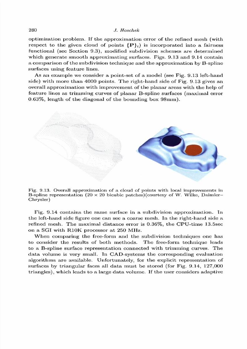
8/3/2019 Multivariate Approximation
http://slidepdf.com/reader/full/multivariate-approximation 290/296
280 J. Hoschek
optimisation problem. If the approximation error of the refined mesh (with
respect to the given cloud of points {P}i) is incorporated into a fairness
functional (see Section 9.3), modified subdivision schemes are determined
which generate smooth approximating surfaces. Figs. 9.13 and 9.14 contain
a comparison of the subdivision technique and the approximation by B-spline
surfaces using feature lines.
As an example we consider a point-set of a model (see Fig. 9.13 left-hand
side) with more than 4000 points. The right-hand side of Fig. 9.13 gives an
overall approximation with improvement of the planar areas with the help of
feature lines as trimming curves of planar B-spline surfaces (maximal error
0.63%, length of the diagonal of the bounding box 98mm).
Fig. 9.13. Overall approximation of a cloud of points with local improvements inB-spline representation (20 x 20 bicubic patches) (courtesy of W. Wilke, Daimler-Chrysler)
Fig . 9.14 contains the same surface in a subdivision approx imation. In
the left-hand side figure one can see a coarse mesh. In the right-hand side a
refined mesh. The maximal distance error is 0.36%, the CPU-time 13.5sec
on a SGI with R10K processor at 250 MHz.
When comparing the free-form and the subdivision techniques one has
to consider the results of bo th m ethods. Th e free-form technique leads
to a B-spline surface representation connected with trimming curves. The
dat a volume is very small. In CAD-systems the corresponding evaluation
algorithm s are available. Unfortunately, for the explicit representation of
surfaces by triangular faces all data must be stored (for Fig. 9.14, 127,000
triangles), which leads to a large data volume. If the user considers adaptive
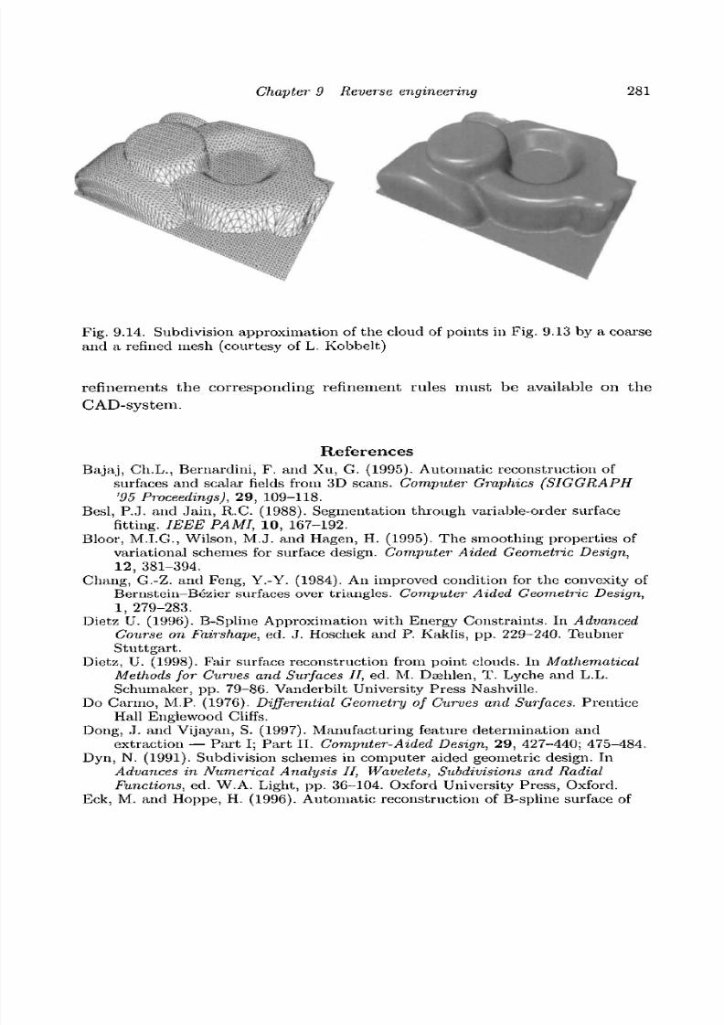
8/3/2019 Multivariate Approximation
http://slidepdf.com/reader/full/multivariate-approximation 291/296
Chapter 9 Reverse engineering 281
Fig. 9.14. Subdivision approxim ation of the cloud of po ints in Fig . 9.13 by a coarseand a refined mesh (courtesy of L. Kobbelt)
refinements the corresponding refinement rules must be available on the
CAD- sys t em.
References
Bajaj, Ch.L., Bernardini, F. and Xu, G. (1995). Automatic reconstruction ofsurfaces and scalar fields from 3D scans. Computer Graphics (SIGGRAPH'95 Proceedings), 29, 109-118.
Besl, P.J. and Jain, R.C. (1988). Segmentation through variable-order surfacefitting. IEEE PAMI, 10, 167-192.
Bloor, M.I.G., Wilson, M.J. and Hagen, H. (1995). The smoothing properties ofvariational schemes for surface design. Computer Aided Geometric Design,
12, 381-394.Chang, G.-Z. and Feng, Y.-Y. (1984). An improved condition for the convexity of
Bernstein-Bezier surfaces over triangles. Computer Aided Geometric Design,1, 279-283.
Dietz U. (1996). B-Spline Approximation with Energy Constraints. In AdvancedCourse on Fairshape, ed. J. Hoschek and P. Kaklis, pp. 229-240. TeubnerStuttgart .
Dietz, U. (1998). Fair surface reconstruction from point clouds. In MathematicalMethods for Curves and Surfaces II, ed. M. Daehlen, T. Lyche and L.L.Schumaker, pp. 79-86. Vanderbilt University Press Nashville.
Do Carmo, M.P. (1976). Differential Geometry of Curves and Surfaces. PrenticeHall Englewood Cliffs.
Dong, J. and Vijayan, S. (1997). Manufacturing feature determination andextraction — Part I; Part II. Computer-Aided Design, 29 , 427-440; 475-484.
Dyn, N. (1991). Subdivision schemes in computer aided geometric design. InAdvan ces in Numerical Analysis II, Wavelets, Subdivisions and RadialFunctions, ed. W.A. Light, pp. 36-104. Oxford University Press, Oxford.
Eck, M. and Hoppe, H. (1996). Automatic reconstruction of B-spline surface of

8/3/2019 Multivariate Approximation
http://slidepdf.com/reader/full/multivariate-approximation 292/296
282 J. Hoschek
arbitrary topological type. Com puter Graphics (SIGGR APH '96Proceedings), 30, 325-334.
Eck, M., DeRose, T., Duchamp, T., Hoppe, H., Lounsbery, M. and Stuetzle, W.(1995). Multiresolution analysis on arbitrary meshes. Com puter Graphics(SIGGR APH '95 Proceedings), 29, 173-182.
Edelsbrunner, H. and Miicke, E. (1994). Three-dimensional alpha shapes. ACMTrans. Graphics, 13, 43-72.
Elsasser, B. and Hoschek, J. (1996). Approximation of digitized points by surfacesof revolution. Comput. & Graphics 20, 85-94.
Farin, G. (1996). Curves and Surfaces for CAG D - A Practical Guide, 4th ed.Academic Press, New York.
Fletcher, R. (1990). Practical Methods of Optimisation. Wiley-Interscience,
Chichester.Greiner, G. (1994). Variational design and fairing of spline surfaces. Computer
Graphics Forum, 13, 143-154.Guo, B. (1997). Surface reconstruction: from points to splines. Computer-Aided
Design, 29, 269-277.Haberiicker, P. (1991). Digitale Bildverarbeitung. Hansa Verlag, Hamburg.Hadenfeld, J. (1995). Local energy fairing of B-spline surfaces. In Mathematical
Methods for Curves and Surfaces, ed. M. Dashlen, T. Lyche and L.L.Schumaker, pp. 203-212. Vanderbilt University Press, Nashville.
Hagen, H. and Schulze, G. (1987). Automatic smoothing with geometric surface
patches. Computer Aided Geometric Design, 4, 231-235.Hoppe, H., DeRose, T., Duchamp, T., McDonald, J. and Stuetzle, W. (1992).
Surface reconstruction from unorganized points. Comp uter Graphics(SIGGR APH '92 Proceedings), 26, 71-78.
Hoschek, J. (1983). Dual Bezier curves and surfaces. In Surfaces in ComputerAided Geometric Design, ed. R.E. Barnhill and W. Boehm, pp. 147-156.North Holland, Amsterdam.
Hoschek, J. and Dietz, U. (1996). Smooth B-spline surface approximation toscattered data. In Reverse Engineering, ed. J. Hoschek and W. Dankwort, pp.143-152. Teubner, Stuttgart.
Hoschek, J. Dietz, U. and Wilke, W. (1998). A geometric concept of reverseengineering of shape: Approximation and feature lines. In MathematicalMethods for Curves and Surfaces II, ed. M. Dsehlen, T. Lyche and L.L.Schumaker, pp. 253-262. Vanderbilt University Press, Nashville.
Hoschek, J. and Jiittler, B. (1999). Techniques for a fair and shape-preservingsurface fitting with tensor-product B-splines. In Shape PreservingRepresentations in Computer Aided Design, ed. J.M. Pena. Nova SciencePublishers, New York.
Hoschek, J. and Lasser, D. (1993). Fundamentals of Computer Aided GeometricDesign. AK Peters, Wellesley.
Hoschek, J. and Schneider, F.-J. (1992). Approximate spline conversion forintegral and rational Bezier and B-spline surfaces. In Geometry Processing forDesign and Manufacturing, ed. R.E. Barnhill, pp. 45-86. SIAM, Philadelphia.
Hoschek, J. and Schneider, M. (1997). Interpolation and approximation withdevelopable surfaces. In Curves and Surfaces with Applications in CAGD, ed .A. Le Mehaute, C. Rabut and L.L. Schumaker, pp. 185-203. VanderbiltUniversity Press, Nashville.
Hoschek, J. and Schwanecke U. (1998). Interpolation and approximation with

8/3/2019 Multivariate Approximation
http://slidepdf.com/reader/full/multivariate-approximation 293/296
Chap ter 9 Reverse engineering 283
ruled surfaces. In The Mathematics of Surfaces VIII, ed. R. Cripps, pp.213-232. Information Geometers, Winchester.
Jiittler, B. (1997a). Linear convexity conditions for parametric tensor-productBezier surface patches. In The Mathematics of Surfaces VII, ed. T.N.T.Goodman and R. Martin, pp. 189-208. Information Geometers, Winchester.
Jiittler, B. (1997b). Surface fitting using convex tensor-product splines. J.Comput. App. Math., 84, 23-44.
Jiittler, B. (1998). Convex surface fitting with tensor-product Bezier surfaces. In
Mathema tical Methods for Curves and Surfaces II, ed. M. Dsehlen, T. Lycheand L.L. Schumaker, pp. 263-270. Vanderbilt University Press, Nashville.
Kass, M., Witkin, A. and Terzopuolos, D. (1987). Snakes: active contour models.
Proceedings of the First International Conference on Computer Vision, 1,
259-269.Kobbelt, L. (1996a). A variational approach to subdivision. Comp uter Aided
Geom etric Design, 13, 743-761.Kobbelt, L. (1996b) Interpolatory subdivision on open quadrilateral nets with
arbitrary topology. Computer Graphics Forum, 15, Eurographics '96Conference Issue, 409-420.
Kobbelt, L. (1997). Discrete fairing. In The Mathematics of Surfaces VII, ed.
T.N.T Goodman and R. Martin, pp. 101-131. Information Geometers,Winchester.
Kobbelt, L. (1998). Variational design with parametric meshes of arbitrary
topology. In Creating fair and shape preserving curves and surfaces, ed. H.Nowacki and P. Kaklis, pp. 189-198. Teubner, Stuttgart.
Kobbelt, L. (1999) Reverse engineering based on subdivision surfaces. Privatecommunication.
Lang, J. and Roschel, O. (1992). Developable (l,n) Bezier surfaces. Computer
Aided Geometric Design, 9, 291-298.Loop, C. and DeRose, T. (1990). Generalised B-spline surfaces of arbitrary
topology. Com puter Graphics (SIGGR APH '90 Proceedings) 24, 347-357.Lukacs, G. and Andor, L. (1998). Computing natural division lines on free-form
surfaces based on measured data. In Mathematical M ethods for Curves andSurfaces II, ed. M. Daehlen, T. Lyche and L.L. Schumaker, pp. 319-326.Vanderbilt University Press, Nashville.
Lukacs, G., Marshall, D. and Martin, R. (1998). Faithful least-squares fitting ofspheres, cylinders, cones and tori. In Computer Vision-ECCV, ed. H.Burkhardt and B. Neumann, pp. 671-686. Lecture Notes in ComputerScience, 1406, Springer-Verlag, Heidelberg.
Milroy, M.J., Bradley, C. and Vickers, G.W. (1997). Segmentation of awrap-around model using an active contour. Computer-Aided Design, 29,299-320.
Moreton, H.P. and Sequin, C.H. (1992). Functional optimisation for fair surfacedesign. Com puter Graphics (SIGGR APH '92 Proceedings), 26, 167-176.Peters, J. (1995) Biquartic C
1-surface splines over irregular meshes.
Computer-Aided Design, 27, 895-903.Pottmann, H., Chen, H.-Y. and Lee, I.-K. (1998a). Approximation by profile
surfaces. In The Mathematics of Surfaces VIII, ed. R. Cripps, pp. 17-36.Information Geometers, Winchester.
Pottmann, H., Peternell, M. and Ravani, B. (1998b). Approximation in line space.
8/3/2019 Multivariate Approximation
http://slidepdf.com/reader/full/multivariate-approximation 294/296
284 J. Hoschek
In Advances in Robot Kinematics: Analysis and C ontrol, ed. J. Lenarcic andM. Husty, pp. 403-412. Kluwer, Dordrecht.
Pottmann, H. and Randrup, T. (1998). Rotational and helical surfaceapproximation for reverse engineering. Computing, 60, 307-322.
Pottmann, H. and Wallner, J. (1999). Approximation algorithms for developablesurfaces. Computer Aided Geometric Design. To be published in 1999.
Rando, T. and Roulier, J.A. (1991). Designing faired parametric surfaces.Computer-Aided Design, 23 , 492-497.
Randrup, T. (1998). Reverse engineering methodology to recognize and enhance
manufacturability of surfaces — with examples from shipbuilding. PhDThesis, Technical University of Denmark, Lyngby.
Sapidis, N.S. and Besl, P.J. (1995). Direct construction of polynomial surfaces
from dense range images through region growing. ACM Trans. Graphics, 14,171-200.
Sarkar, B. and Menq, C.H. (1991). Smooth-surface approximation and reverseengineering. Computer-Aided Design, 23, 623-628.
Schneider, M. (1998). Interpolation with developable strip-surfaces consisting ofcylinders and cones. In Mathematical M ethods for Curves and Surfaces II, ed .M. Daehlen, T. Lyche and L.L. Schumaker, pp. 437-444. VanderbiltUniversity Press, Nashville.
Shewchuck, J.R. (1995). Triangle - a two-dimensional quality mesh generator andDelaunay Triangulator. Tech. Report Carnegie Mellon University, Pittsburgh.
Sinha, S.S. and Schunck, B.G. (1992). A two-stage algorithm for discontinuity-preserving surface reconstruction. IEEE Trans, on Pattern A nalysis andMachine Intelligence, 14, 36-55.
Speer, T., Kuppe, M., and Hoschek, J. (1998). Global reparametrization of curveapproximation. Computer Aided Geometric Design, 15, 869-878.
Vanderbei, R. (1992). LOQO Version 1.08, available via anonymous ftp frome l i b . z i b - b e r l i n . d e a t / p u b / o p t - n e t/ s o ft w a r e / lo q o / 1 . 0 8 .
Varady, T., Martin, R.R. and Cox, J. (1997). Reverse engineering of geometricmodels - an introduction. Computer-Aided Design, 29, 255-268.
Welch, W. and Witkin, A. (1992). Variational surface modeling. Computer
Graphics (SIGGR APH '92 Proceedings), 26, 157-166.Wilke, W. (2000). Segmentierung und approximation grofier punktviolken. PhDThesis, Darmstadt University of Technology.
Willemans, K. and Dierckx, P. (1994). Surface fitting using convex Powell—Sabinsplines. J. Comput. Appl. Math., 56, 263-282.
Ye, X., Jackson, T.R. and Patrikalakis, N.M. (1996). Geometric design offunctional surfaces. Computer-Aided Design, 28, 741-752.

8/3/2019 Multivariate Approximation
http://slidepdf.com/reader/full/multivariate-approximation 295/296
Index
adaptive
methods, 59, 190
partitions, 192, 193, 210
splitting, 192
analysis operator, 115-117, 227
angular variation, 258-261
approximation
N-term, 189, 190, 196, 198, 210
order, 38, 44, 58, 73, 74, 81, 82, 85, 86,
88-90, 98, 104, 105
B-splino, 85, 153, 157-160, 162, 163, 165,
171-175, 182, 185, 214, 219, 266, 272
Grain matrices, 159, 185
surfaces, 262, 280
B-wavelet, 153, 154, 164, 166, 168-171, 174,
182-184
Besov spaces, 195, 196, 212
Bessel
function, 7-9, 13, 14, 19
systems, 129-131, 144
bottom-up method, 253
bracket product, 75, 76, 83, 86, 127, 128,
132
Cesaro means, 47
collocation matrix, 31, 158, 159
compact Riemannian manifold, 50, 51
completely monotone, 3, 5, 6
conditionally positive definite, 26, 30, 38, 40,
52
continuous wavelet transform (CWT), 45, 59,
60
data compression, 188, 190, 203, 211
developable surfaces, 276-278
dilation matrix, 87, 88, 103-106
discrete wavelet transform (DWT), 45, 59,
60
dual basis, 117, 120, 121, 123, 135, 143
energy constraints, 262, 272
erosion operator, 260
error
indicators, 207
tolerance, 253, 262, 272
fairness functional, 264, 265, 280
fast multipole methods, 33, 36
fiberization, 115, 132, 142, 143
Fourier transform, 5-9, 18, 19, 21, 30, 32, 45,
64, 74, 76, 112, 113, 117, 119, 124, 134,
142, 143, 203
frames, 114, 115, 122, 129, 132, 142, 143, 213,
217-219, 229
free-form surface, 253, 276, 279
free-knot splines, 198
FSI space, 73, 75, 76, 81, 82, 85, 104, 106, 113,
114, 132, 142, 143
Gelfand transform, 124
Gram matrices, 159, 176, 178, 185
Gramian analysis, 143
Holder spaces, 192
hierarchy, 218, 225, 234, 236, 242
homogeneous harmonic polynomial, 46
interpolation, 25, 39, 44, 45, 49, 52, 53, 50, 133
scattered data, 53
knot
insertion, 159, 160, 162, 198, 273
multiplicity of, 164, 166, 182
Laplace-Beltrami operator, 46, 51, 61, 62
Legendre polynomials, 47, 49, 53
linear independence
local, 115, 125, 145, 146
Marcinkiewicz-Zygmund inequality, 57, 67,
68
matrix
collocation, 158, 159
dilation, 87, 88, 103-106
285

8/3/2019 Multivariate Approximation
http://slidepdf.com/reader/full/multivariate-approximation 296/296