Multivariate analysis of extremely large ToFSIMS imaging ... · image for PCA analysis, even though...
8
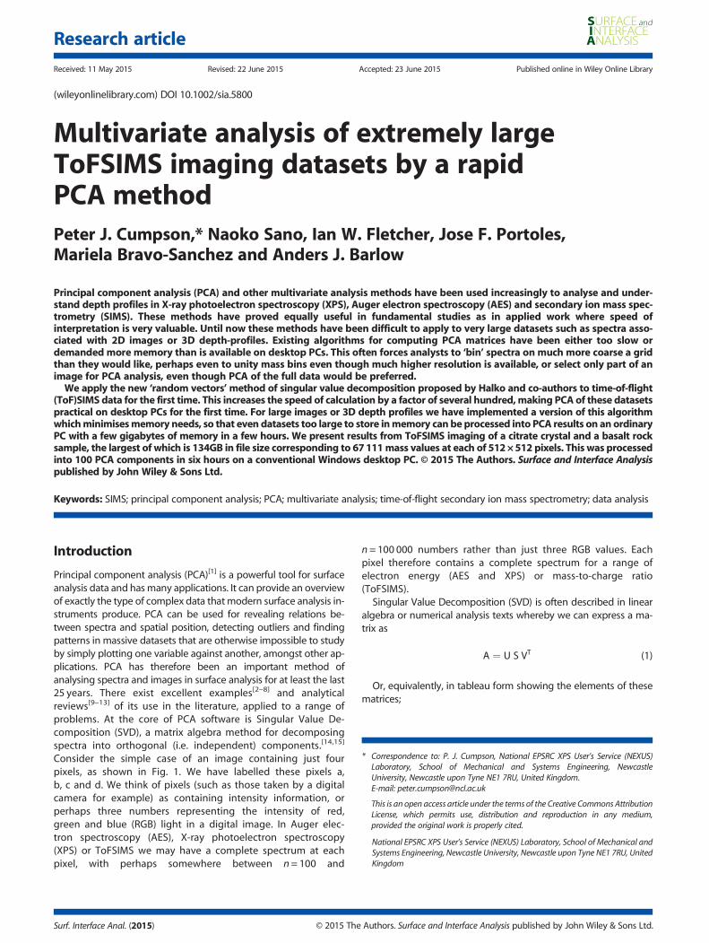
Multivariate analysis of extremely large ToFSIMS imaging datasets by a rapid PCA method Peter J. Cumpson,* Naoko Sano, Ian W. Fletcher, Jose F. Portoles, Mariela Bravo-Sanchez and Anders J. Barlow Principal component analysis (PCA) and other multivariate analysis methods have been used increasingly to analyse and under- stand depth profiles in X-ray photoelectron spectroscopy (XPS), Auger electron spectroscopy (AES) and secondary ion mass spec- trometry (SIMS). These methods have proved equally useful in fundamental studies as in applied work where speed of interpretation is very valuable. Until now these methods have been difficult to apply to very large datasets such as spectra asso- ciated with 2D images or 3D depth-profiles. Existing algorithms for computing PCA matrices have been either too slow or demanded more memory than is available on desktop PCs. This often forces analysts to ‘bin’ spectra on much more coarse a grid than they would like, perhaps even to unity mass bins even though much higher resolution is available, or select only part of an image for PCA analysis, even though PCA of the full data would be preferred. We apply the new ‘random vectors’ method of singular value decomposition proposed by Halko and co-authors to time-of-flight (ToF)SIMS data for the first time. This increases the speed of calculation by a factor of several hundred, making PCA of these datasets practical on desktop PCs for the first time. For large images or 3D depth profiles we have implemented a version of this algorithm which minimises memory needs, so that even datasets too large to store in memory can be processed into PCA results on an ordinary PC with a few gigabytes of memory in a few hours. We present results from ToFSIMS imaging of a citrate crystal and a basalt rock sample, the largest of which is 134GB in file size corresponding to 67 111 mass values at each of 512 × 512 pixels. This was processed into 100 PCA components in six hours on a conventional Windows desktop PC. © 2015 The Authors. Surface and Interface Analysis published by John Wiley & Sons Ltd. Keywords: SIMS; principal component analysis; PCA; multivariate analysis; time-of-flight secondary ion mass spectrometry; data analysis Introduction Principal component analysis (PCA) [1] is a powerful tool for surface analysis data and has many applications. It can provide an overview of exactly the type of complex data that modern surface analysis in- struments produce. PCA can be used for revealing relations be- tween spectra and spatial position, detecting outliers and finding patterns in massive datasets that are otherwise impossible to study by simply plotting one variable against another, amongst other ap- plications. PCA has therefore been an important method of analysing spectra and images in surface analysis for at least the last 25 years. There exist excellent examples [2–8] and analytical reviews [9–13] of its use in the literature, applied to a range of problems. At the core of PCA software is Singular Value De- composition (SVD), a matrix algebra method for decomposing spectra into orthogonal (i.e. independent) components. [14,15] Consider the simple case of an image containing just four pixels, as shown in Fig. 1. We have labelled these pixels a, b, c and d. We think of pixels (such as those taken by a digital camera for example) as containing intensity information, or perhaps three numbers representing the intensity of red, green and blue (RGB) light in a digital image. In Auger elec- tron spectroscopy (AES), X-ray photoelectron spectroscopy (XPS) or ToFSIMS we may have a complete spectrum at each pixel, with perhaps somewhere between n = 100 and n = 100 000 numbers rather than just three RGB values. Each pixel therefore contains a complete spectrum for a range of electron energy (AES and XPS) or mass-to-charge ratio (ToFSIMS). Singular Value Decomposition (SVD) is often described in linear algebra or numerical analysis texts whereby we can express a ma- trix as A ¼ USV T (1) Or, equivalently, in tableau form showing the elements of these matrices; * Correspondence to: P. J. Cumpson, National EPSRC XPS User’s Service (NEXUS) Laboratory, School of Mechanical and Systems Engineering, Newcastle University, Newcastle upon Tyne NE1 7RU, United Kingdom. E-mail: [email protected] This is an open access article under the terms of the Creative Commons Attribution License, which permits use, distribution and reproduction in any medium, provided the original work is properly cited. National EPSRC XPS User’s Service (NEXUS) Laboratory, School of Mechanical and Systems Engineering, Newcastle University, Newcastle upon Tyne NE1 7RU, United Kingdom Surf. Interface Anal. (2015) © 2015 The Authors. Surface and Interface Analysis published by John Wiley & Sons Ltd. Research article Received: 11 May 2015 Revised: 22 June 2015 Accepted: 23 June 2015 Published online in Wiley Online Library (wileyonlinelibrary.com) DOI 10.1002/sia.5800
Transcript of Multivariate analysis of extremely large ToFSIMS imaging ... · image for PCA analysis, even though...
Research article
Received: 11 May 2015 Revised: 22 June 2015 Accepted: 23 June 2015 Published online in Wiley Online Library
(wileyonlinelibrary.com) DOI 10.1002/sia.5800
Multivariate analysis of extremely largeToFSIMS imaging datasets by a rapidPCA methodPeter J. Cumpson,* Naoko Sano, Ian W. Fletcher, Jose F. Portoles,Mariela Bravo-Sanchez and Anders J. Barlow
Principal component analysis (PCA) and other multivariate analysis methods have been used increasingly to analyse and under-stand depth profiles in X-ray photoelectron spectroscopy (XPS), Auger electron spectroscopy (AES) and secondary ion mass spec-trometry (SIMS). These methods have proved equally useful in fundamental studies as in applied work where speed ofinterpretation is very valuable. Until now these methods have been difficult to apply to very large datasets such as spectra asso-ciated with 2D images or 3D depth-profiles. Existing algorithms for computing PCA matrices have been either too slow ordemanded more memory than is available on desktop PCs. This often forces analysts to ‘bin’ spectra on much more coarse a gridthan they would like, perhaps even to unity mass bins even though much higher resolution is available, or select only part of animage for PCA analysis, even though PCA of the full data would be preferred.
We apply the new ‘random vectors’method of singular value decomposition proposed by Halko and co-authors to time-of-flight(ToF)SIMS data for the first time. This increases the speed of calculation by a factor of several hundred,making PCA of these datasetspractical on desktop PCs for the first time. For large images or 3D depth profiles we have implemented a version of this algorithmwhichminimisesmemory needs, so that even datasets too large to store inmemory can be processed into PCA results on an ordinaryPC with a few gigabytes of memory in a few hours. We present results from ToFSIMS imaging of a citrate crystal and a basalt rocksample, the largest of which is 134GB in file size corresponding to 67111mass values at each of 512×512 pixels. This was processedinto 100 PCA components in six hours on a conventional Windows desktop PC. © 2015 The Authors. Surface and Interface Analysispublished by John Wiley & Sons Ltd.
Keywords: SIMS; principal component analysis; PCA; multivariate analysis; time-of-flight secondary ion mass spectrometry; data analysis
* Correspondence to: P. J. Cumpson, National EPSRC XPS User’s Service (NEXUS)Laboratory, School of Mechanical and Systems Engineering, NewcastleUniversity, Newcastle upon Tyne NE1 7RU, United Kingdom.E-mail: [email protected]
This is an open access article under the terms of the Creative Commons AttributionLicense, which permits use, distribution and reproduction in any medium,provided the original work is properly cited.
National EPSRC XPS User’s Service (NEXUS) Laboratory, School of Mechanical andSystems Engineering, Newcastle University, Newcastle upon Tyne NE1 7RU, UnitedKingdom
Introduction
Principal component analysis (PCA)[1] is a powerful tool for surfaceanalysis data and hasmany applications. It can provide an overviewof exactly the type of complex data that modern surface analysis in-struments produce. PCA can be used for revealing relations be-tween spectra and spatial position, detecting outliers and findingpatterns in massive datasets that are otherwise impossible to studyby simply plotting one variable against another, amongst other ap-plications. PCA has therefore been an important method ofanalysing spectra and images in surface analysis for at least the last25 years. There exist excellent examples[2–8] and analyticalreviews[9–13] of its use in the literature, applied to a range ofproblems. At the core of PCA software is Singular Value De-composition (SVD), a matrix algebra method for decomposingspectra into orthogonal (i.e. independent) components.[14,15]
Consider the simple case of an image containing just fourpixels, as shown in Fig. 1. We have labelled these pixels a,b, c and d. We think of pixels (such as those taken by a digitalcamera for example) as containing intensity information, orperhaps three numbers representing the intensity of red,green and blue (RGB) light in a digital image. In Auger elec-tron spectroscopy (AES), X-ray photoelectron spectroscopy(XPS) or ToFSIMS we may have a complete spectrum at eachpixel, with perhaps somewhere between n= 100 and
Surf. Interface Anal. (2015) © 2015 The
n = 100 000 numbers rather than just three RGB values. Eachpixel therefore contains a complete spectrum for a range ofelectron energy (AES and XPS) or mass-to-charge ratio(ToFSIMS).
Singular Value Decomposition (SVD) is often described in linearalgebra or numerical analysis texts whereby we can express a ma-trix as
A ¼ U S VT (1)
Or, equivalently, in tableau form showing the elements of thesematrices;
Authors. Surface and Interface Analysis published by John Wiley & Sons Ltd.
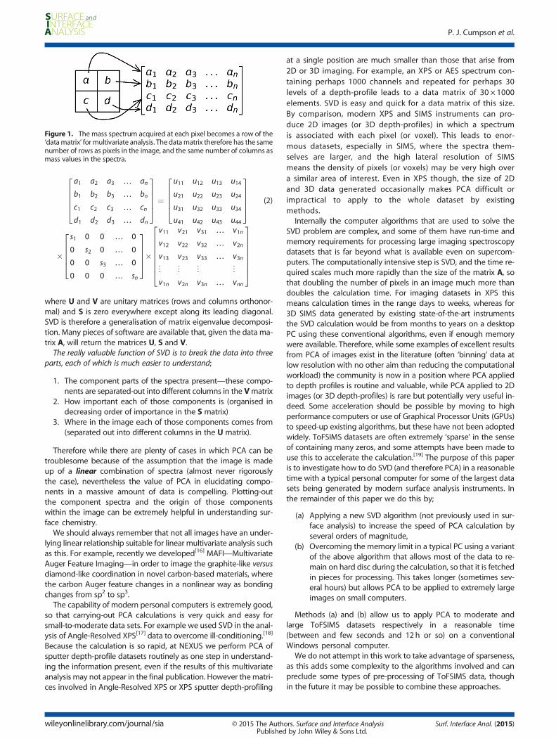
Figure 1. The mass spectrum acquired at each pixel becomes a row of the‘datamatrix’ for multivariate analysis. The datamatrix therefore has the samenumber of rows as pixels in the image, and the same number of columns asmass values in the spectra.
P. J. Cumpson et al.
a1 a2 a3 … an
b1 b2 b3 … bn
c1 c2 c3 … cn
d1 d2 d3 … dn
26664
37775 ¼
u11 u12 u13 u14
u21 u22 u23 u24
u31 u32 u33 u34
u41 u42 u43 u44
26664
37775
�
s1 0 0 … 0
0 s2 0 … 0
0 0 s3 … 0
0 0 0 … sn
26664
37775�
v11 v21 v31 … v1n
v12 v22 v32 … v2n
v13 v23 v33 … v3n
⋮ ⋮ ⋮ ⋮
v1n v2n v3n … vnn
26666664
37777775
(2)
where U and V are unitary matrices (rows and columns orthonor-mal) and S is zero everywhere except along its leading diagonal.SVD is therefore a generalisation of matrix eigenvalue decomposi-tion. Many pieces of software are available that, given the data ma-trix A, will return the matrices U, S and V.The really valuable function of SVD is to break the data into three
parts, each of which is much easier to understand;
1. The component parts of the spectra present—these compo-nents are separated-out into different columns in the Vmatrix
2. How important each of those components is (organised indecreasing order of importance in the S matrix)
3. Where in the image each of those components comes from(separated out into different columns in the U matrix).
Therefore while there are plenty of cases in which PCA can betroublesome because of the assumption that the image is madeup of a linear combination of spectra (almost never rigorouslythe case), nevertheless the value of PCA in elucidating compo-nents in a massive amount of data is compelling. Plotting-outthe component spectra and the origin of those componentswithin the image can be extremely helpful in understanding sur-face chemistry.We should always remember that not all images have an under-
lying linear relationship suitable for linear multivariate analysis suchas this. For example, recently we developed[16] MAFI—MultivariateAuger Feature Imaging—in order to image the graphite-like versusdiamond-like coordination in novel carbon-based materials, wherethe carbon Auger feature changes in a nonlinear way as bondingchanges from sp2 to sp3.The capability of modern personal computers is extremely good,
so that carrying-out PCA calculations is very quick and easy forsmall-to-moderate data sets. For example we used SVD in the anal-ysis of Angle-Resolved XPS[17] data to overcome ill-conditioning.[18]
Because the calculation is so rapid, at NEXUS we perform PCA ofsputter depth-profile datasets routinely as one step in understand-ing the information present, even if the results of this multivariateanalysis may not appear in the final publication. However thematri-ces involved in Angle-Resolved XPS or XPS sputter depth-profiling
wileyonlinelibrary.com/journal/sia © 2015 The AuthPublished
at a single position are much smaller than those that arise from2D or 3D imaging. For example, an XPS or AES spectrum con-taining perhaps 1000 channels and repeated for perhaps 30levels of a depth-profile leads to a data matrix of 30 × 1000elements. SVD is easy and quick for a data matrix of this size.By comparison, modern XPS and SIMS instruments can pro-duce 2D images (or 3D depth-profiles) in which a spectrumis associated with each pixel (or voxel). This leads to enor-mous datasets, especially in SIMS, where the spectra them-selves are larger, and the high lateral resolution of SIMSmeans the density of pixels (or voxels) may be very high overa similar area of interest. Even in XPS though, the size of 2Dand 3D data generated occasionally makes PCA difficult orimpractical to apply to the whole dataset by existingmethods.
Internally the computer algorithms that are used to solve theSVD problem are complex, and some of them have run-time andmemory requirements for processing large imaging spectroscopydatasets that is far beyond what is available even on supercom-puters. The computationally intensive step is SVD, and the time re-quired scales much more rapidly than the size of the matrix A, sothat doubling the number of pixels in an image much more thandoubles the calculation time. For imaging datasets in XPS thismeans calculation times in the range days to weeks, whereas for3D SIMS data generated by existing state-of-the-art instrumentsthe SVD calculation would be from months to years on a desktopPC using these conventional algorithms, even if enough memorywere available. Therefore, while some examples of excellent resultsfrom PCA of images exist in the literature (often ‘binning’ data atlow resolution with no other aim than reducing the computationalworkload) the community is now in a position where PCA appliedto depth profiles is routine and valuable, while PCA applied to 2Dimages (or 3D depth-profiles) is rare but potentially very useful in-deed. Some acceleration should be possible by moving to highperformance computers or use of Graphical Processor Units (GPUs)to speed-up existing algorithms, but these have not been adoptedwidely. ToFSIMS datasets are often extremely ‘sparse’ in the senseof containing many zeros, and some attempts have been made touse this to accelerate the calculation.[19] The purpose of this paperis to investigate how to do SVD (and therefore PCA) in a reasonabletime with a typical personal computer for some of the largest datasets being generated by modern surface analysis instruments. Inthe remainder of this paper we do this by;
(a) Applying a new SVD algorithm (not previously used in sur-face analysis) to increase the speed of PCA calculation byseveral orders of magnitude,
(b) Overcoming the memory limit in a typical PC using a variantof the above algorithm that allows most of the data to re-main on hard disc during the calculation, so that it is fetchedin pieces for processing. This takes longer (sometimes sev-eral hours) but allows PCA to be applied to extremely largeimages on small computers.
Methods (a) and (b) allow us to apply PCA to moderate andlarge ToFSIMS datasets respectively in a reasonable time(between and few seconds and 12h or so) on a conventionalWindows personal computer.
We do not attempt in this work to take advantage of sparseness,as this adds some complexity to the algorithms involved and canpreclude some types of pre-processing of ToFSIMS data, thoughin the future it may be possible to combine these approaches.
ors. Surface and Interface Analysisby John Wiley & Sons Ltd.
Surf. Interface Anal. (2015)

Figure 3. (a) Total ion ToFSIMS image, in positive ion mode, of a sodiumcitrate crystal. The field of view is 1mm×1mm. Also shown is (b), an opticalimage of a similar but not the same crystal. These crystals are typicallyaround 0.5 to 1.0mm in size. This figure is in colour in the online version.
Figure 2. Calculation times recorded for PCA of complete 64 × 64 pixelimages having increasing spectra associated with each pixel. Calculationswere performed with three different algorithms in two common numericalanalysis packages (Octave and Matlab), (a) Octave xGESVD, (b) OctavexGESSD, (c) Matlab xGESVD, (d) Octave, our implementation of Halkoet al.’s algorithm (RV1), (e) Matlab, our implementation of Halko et al.’salgorithm (RV1).
Extremely large ToFSIMS imaging by rapid PCA
Surf. Interface Anal. (2015) © 2015 The Authors. Surface apublished by John Wile
Requirements of surface analysis
We can identify three key requirements of an algorithm suitable forsurface analysis imaging applications;
1. It should be fast for images containing a large number ofpixels and having large spectra in those pixels
2. The memory requirements should be within those availableon easily-accessible PCs,
3. It should be capable of decomposing low-rank data matrices,i.e. we believe that the spectra in the image are made-up of asmall number of factors, almost certainly below 100, and cer-tainly a very small number compared to the total number ofpixels.
Note that there is an extensive literature and recommendationson data pre-processing required in XPS and ToFSIMS, which may in-clude normalisation, mean-centering and Poisson distribution vari-ance correction.[20] While numerically quick and easy it is not thepurpose of this paper to examine them, as they do not affect the pri-mary issue which is the scale of spectral imaging data. The issuesof pre-processing are the same whatever SVD or PCA algorithmis used, and whether the data matrix has 102 elements or 1010.However because the choice of preprocessing method dependson the application, and there are publications that discuss
Figure 4. (a) Positive ion spectrum of sodium citrate. (b) Positive ionspectrum of the substrate (double sided tape).
nd Interface Analysisy & Sons Ltd.
wileyonlinelibrary.com/journal/sia

P. J. Cumpson et al.
preprocessing of surface analytical data in depth,[21,22] it will notbe considered here.
Four SVD algorithms
We will not describe the details of any SVD algorithms here,but from the point of view of the criteria set out above it isworthwhile highlighting the properties of different classes ofalgorithm for performing exactly the same SVD function. Welist these below in the historical order in which they were de-veloped; we will not explain the terminology and acronymshere, which are included simply to facilitate the reader inlooking-up the details of how they work if required. Properlyused, each of these algorithms delivers the same resultsexcept for small truncation and rounding errors intrinsic tonumerical computation, though the time taken and memoryrequired during the calculation can be very different. We willuse the terminology of LAPACK[23] in describing them, as thisis probably the most widely used numerical subroutinelibrary.
Figure 5. PCA results of sodium citrate. The size of each image component is 1m
wileyonlinelibrary.com/journal/sia © 2015 The AuthorsPublished b
1. Householder reduction to bidiagonal form, followed by QRand shifts[24,25] to eliminate off-diagonal elements. This is im-plemented in the routine xGESVD in LAPACK. This type of SVDalgorithm has been used extensively since the time of its firstdescription in the literature by Golub, Kahan and Reinsch inthe period 1965 to 1970.
2. A divide and conquer algorithm[26] (implemented in the rou-tine xGESDD in LAPACK). This is faster for very large matricesthan algorithm 1 (so is closer to what we need for surface an-alytical imaging), but uses more memory. This was describedin the literature around 1995 and added to major linear alge-bra libraries in the late 1990s (e.g. LAPACK V3.0 in 1999).
3. A ‘Random vectors’ version of the block Lanczos method be-cause of Halko et al.,[27] and developed as part of his PhDwork.[28] This is a very newmethod, appearing in the literaturearound 2010/2011. Variants of the algorithm are still appearingin the primary numerical analysis literature. Thismethodworkswell for extremely large data matrices, requires that the datamatrix be of low rank (an assumption PCA practitioners alwaysmustmake in any case) and is much faster than algorithm 1 or2 in this limit. We will call this algorithm ‘RV1’
m×1mm, 256 × 256 pixels.
. Surface and Interface Analysisy John Wiley & Sons Ltd.
Surf. Interface Anal. (2015)
Extremely large ToFSIMS imaging by rapid PCA
4. An ‘out-of-core’ variant of algorithm 3 has been demon-strated that greatly reduces memory requirements too. Thisis achieved by organising the numerical steps involved effi-ciently so that the data matrix is operated-upon in pieces,and therefore the whole data matrix need not be in memoryat any one time. We will call this algorithm ‘RV2’
RV1 is themost rapid of these algorithms for large image PCA, butrelies on enough computer memory being available to hold the PCAdata matrix in memory. RV2 is slower because it allows most of thePCA data matrix to reside on disc, loading successive segments ofthis data matrix into memory for processing. Although slower, RV2can process very large datamatrices, and is quite capable of process-ing the largest ToFSIMS datasets on an ordinary PC. The largestdataset we have so far processed in this way occupies 134GB whenuncompressed, and this processing took only around 6h.
Methods 1 and 2 (xGESVD and xGESDD) are widely used, andthese are the algorithms inside the commonly used software suchas Matlab and Octave that perform SVD (and which are therefore
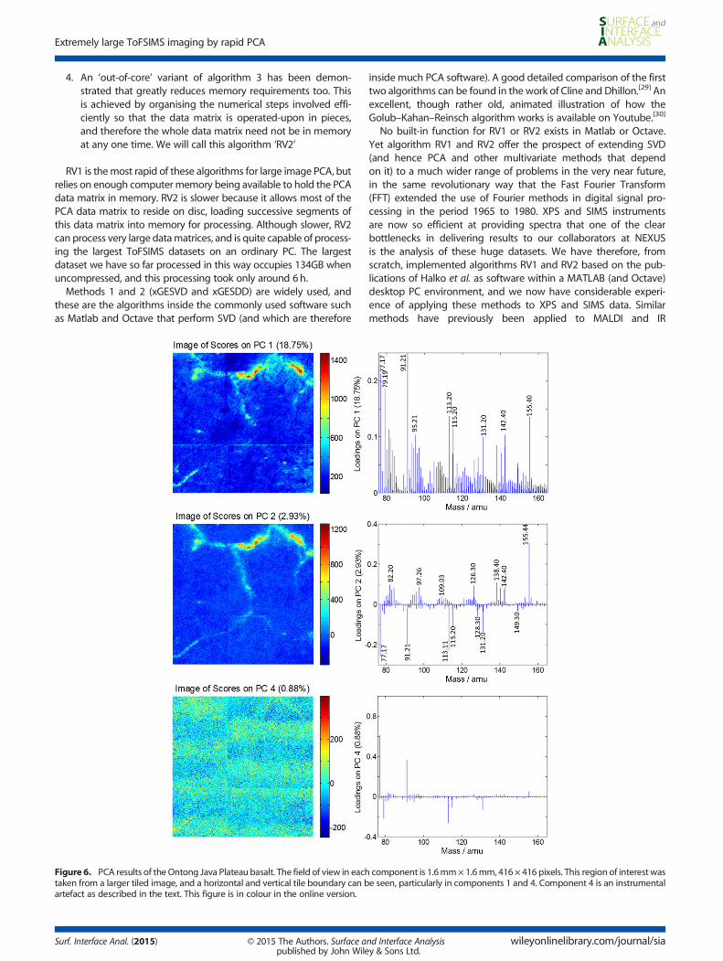
Figure 6. PCA results of the Ontong Java Plateau basalt. The field of view in eachtaken from a larger tiled image, and a horizontal and vertical tile boundary can bartefact as described in the text. This figure is in colour in the online version.
Surf. Interface Anal. (2015) © 2015 The Authors. Surface apublished by John Wile
inside much PCA software). A good detailed comparison of the firsttwo algorithms can be found in the work of Cline and Dhillon.[29] Anexcellent, though rather old, animated illustration of how theGolub–Kahan–Reinsch algorithm works is available on Youtube.[30]
No built-in function for RV1 or RV2 exists in Matlab or Octave.Yet algorithm RV1 and RV2 offer the prospect of extending SVD(and hence PCA and other multivariate methods that dependon it) to a much wider range of problems in the very near future,in the same revolutionary way that the Fast Fourier Transform(FFT) extended the use of Fourier methods in digital signal pro-cessing in the period 1965 to 1980. XPS and SIMS instrumentsare now so efficient at providing spectra that one of the clearbottlenecks in delivering results to our collaborators at NEXUSis the analysis of these huge datasets. We have therefore, fromscratch, implemented algorithms RV1 and RV2 based on the pub-lications of Halko et al. as software within a MATLAB (and Octave)desktop PC environment, and we now have considerable experi-ence of applying these methods to XPS and SIMS data. Similarmethods have previously been applied to MALDI and IR
component is 1.6mm×1.6mm, 416× 416 pixels. This region of interest wase seen, particularly in components 1 and 4. Component 4 is an instrumental
nd Interface Analysisy & Sons Ltd.
wileyonlinelibrary.com/journal/sia
P. J. Cumpson et al.
imaging,[31] and to ICR-MS spectrum data,[32] but we believe thisis the first report of application of them to SIMS.
Time taken by RV1 compared to earlieralgorithms
In Fig. 2 we compare calculation times for a relatively small but use-ful model problem of a 64×64 pixel image having an increasingsize of spectrum associated with each pixel. This logarithmic plot in-dicates roughly power-law dependence of calculation time on thenumber of values in each spectrum. All calculations in this paper, in-cluding these, were performed on a Dell Precision T1700 desktopPC with 16GB of memory and an Intel Xeon E3-1271 CPU, running64-bit Microsoft Windows 7. Matlab R2014a was used for most ofthe work, but we also used the portable version of Octave version3.8.2. No conclusions should be drawn from this work about the rel-ative speed of Matlab compared to Octave, because the ‘portable’version of Octave does not give a fair comparison, instead it is thetrend in calculation time as the spectrum size increases that is im-portant, and this trend is very similar within both the Octave andMatlab platforms. Figure 2 does, however, show strong differencesin speed between the available algorithms.From Fig. 2 we can see that, especially for large spectra, the dif-
ferent algorithms available for calculating the SVD of the same ma-trix differ widely in their speed. In order of increasing speed forlarge matrices these are, (a) Octave xGESVD, (b) Octave xGESSD,(c) Matlab xGESVD, (d) Our implementation of Halko et al.’s algo-rithm (RV1) in Octave and (e) Our implementation of Halkoet al.’s algorithm (RV1) in MATLAB. For images or datasets largerthan those in Fig. 2, only Halko et al.’s algorithm is sufficiently fastfor regular and routine use. In general waiting 20 s for a result (as inthe longest calculation in Fig. 1(c)) is not a problem. Figure 1(e) of-fers the same result in about 0.1 s, a modest time saving. However,extrapolating Fig. 1(c) and Fig. 1(e) to larger problems—perhaps512×512 pixels each with 60 000 mass values or more, is only re-ally practical for the Halko et al. algorithm (which we have calledRV1). Those of us that have tried to perform PCA on large datasetsin the past, and found PCA to be impractically slow or demandingof memory can now reconsider. Halko et al.’s algorithms RV1 andRV2 remove these problems.
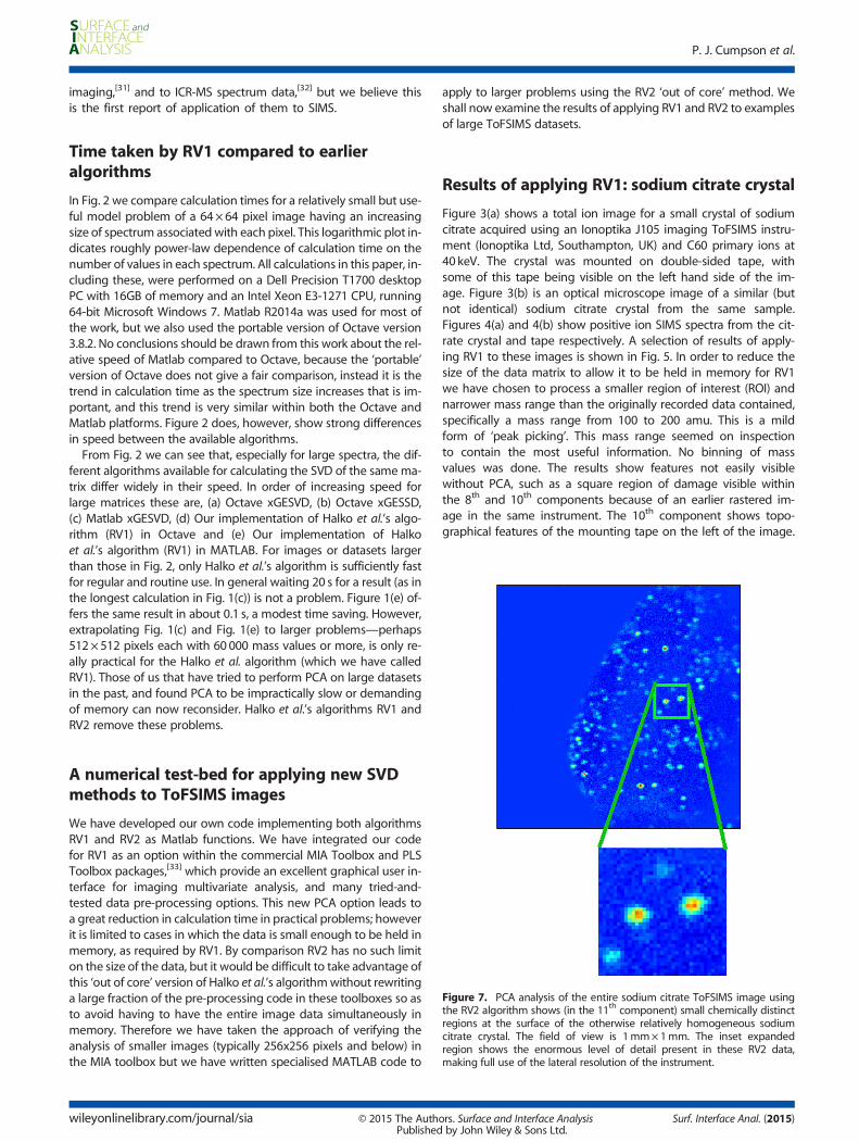
Figure 7. PCA analysis of the entire sodium citrate ToFSIMS image usingthe RV2 algorithm shows (in the 11th component) small chemically distinctregions at the surface of the otherwise relatively homogeneous sodiumcitrate crystal. The field of view is 1mm× 1mm. The inset expandedregion shows the enormous level of detail present in these RV2 data,making full use of the lateral resolution of the instrument.
A numerical test-bed for applying new SVDmethods to ToFSIMS images
We have developed our own code implementing both algorithmsRV1 and RV2 as Matlab functions. We have integrated our codefor RV1 as an option within the commercial MIA Toolbox and PLSToolbox packages,[33] which provide an excellent graphical user in-terface for imaging multivariate analysis, and many tried-and-tested data pre-processing options. This new PCA option leads toa great reduction in calculation time in practical problems; howeverit is limited to cases in which the data is small enough to be held inmemory, as required by RV1. By comparison RV2 has no such limiton the size of the data, but it would be difficult to take advantage ofthis ‘out of core’ version of Halko et al.’s algorithmwithout rewritinga large fraction of the pre-processing code in these toolboxes so asto avoid having to have the entire image data simultaneously inmemory. Therefore we have taken the approach of verifying theanalysis of smaller images (typically 256x256 pixels and below) inthe MIA toolbox but we have written specialised MATLAB code to
wileyonlinelibrary.com/journal/sia © 2015 The AuthPublished
apply to larger problems using the RV2 ‘out of core’ method. Weshall now examine the results of applying RV1 and RV2 to examplesof large ToFSIMS datasets.
Results of applying RV1: sodium citrate crystal
Figure 3(a) shows a total ion image for a small crystal of sodiumcitrate acquired using an Ionoptika J105 imaging ToFSIMS instru-ment (Ionoptika Ltd, Southampton, UK) and C60 primary ions at40 keV. The crystal was mounted on double-sided tape, withsome of this tape being visible on the left hand side of the im-age. Figure 3(b) is an optical microscope image of a similar (butnot identical) sodium citrate crystal from the same sample.Figures 4(a) and 4(b) show positive ion SIMS spectra from the cit-rate crystal and tape respectively. A selection of results of apply-ing RV1 to these images is shown in Fig. 5. In order to reduce thesize of the data matrix to allow it to be held in memory for RV1we have chosen to process a smaller region of interest (ROI) andnarrower mass range than the originally recorded data contained,specifically a mass range from 100 to 200 amu. This is a mildform of ‘peak picking’. This mass range seemed on inspectionto contain the most useful information. No binning of massvalues was done. The results show features not easily visiblewithout PCA, such as a square region of damage visible withinthe 8th and 10th components because of an earlier rastered im-age in the same instrument. The 10th component shows topo-graphical features of the mounting tape on the left of the image.
ors. Surface and Interface Analysisby John Wiley & Sons Ltd.
Surf. Interface Anal. (2015)
Extremely large ToFSIMS imaging by rapid PCA
Results of applying RV1: organic inclusions inbasalt
Basalts from the Ontong Java Plateau possess easily distinguish-able tube-like alteration textures that appear to be of biologicalin origin, but the unambiguous presence of molecular bio-markers or their digenetic products to date has yet to be fullyconfirmed. TofSIMS could be an extremely useful tool in theidentification of these biomarkers. Figure 6 shows PCA resultsfrom applying algorithm RV1 to an edited area of an image ac-quired using 40-keV argon cluster ion as primaries in theIonoptika J105, with a primary spot-size of around 3μm. Fissurescontaining organic material are clear in components 1 and 2.Component 4, however, shows a purely instrumental effect unre-lated to the chemistry of the surface. We believe this to be
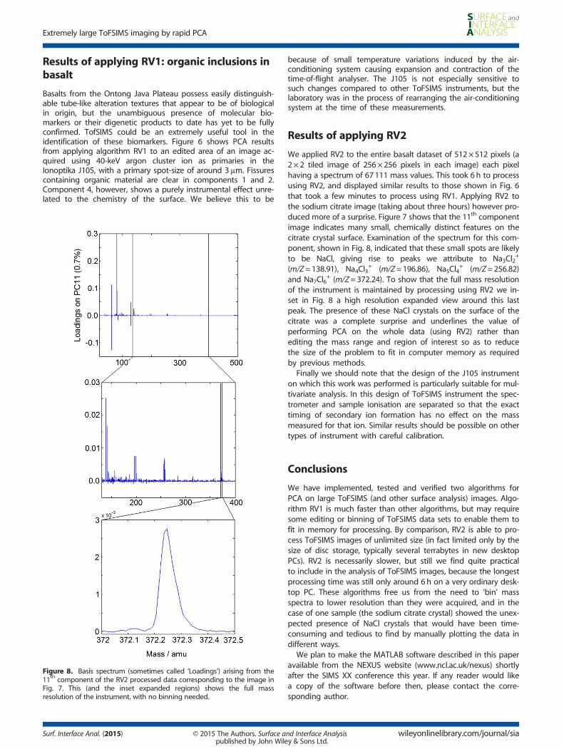
Figure 8. Basis spectrum (sometimes called ‘Loadings’) arising from the11th component of the RV2 processed data corresponding to the image inFig. 7. This (and the inset expanded regions) shows the full massresolution of the instrument, with no binning needed.
Surf. Interface Anal. (2015) © 2015 The Authors. Surface apublished by John Wile
because of small temperature variations induced by the air-conditioning system causing expansion and contraction of thetime-of-flight analyser. The J105 is not especially sensitive tosuch changes compared to other ToFSIMS instruments, but thelaboratory was in the process of rearranging the air-conditioningsystem at the time of these measurements.
Results of applying RV2
We applied RV2 to the entire basalt dataset of 512×512 pixels (a2 × 2 tiled image of 256×256 pixels in each image) each pixelhaving a spectrum of 67111 mass values. This took 6 h to processusing RV2, and displayed similar results to those shown in Fig. 6that took a few minutes to process using RV1. Applying RV2 tothe sodium citrate image (taking about three hours) however pro-duced more of a surprise. Figure 7 shows that the 11th componentimage indicates many small, chemically distinct features on thecitrate crystal surface. Examination of the spectrum for this com-ponent, shown in Fig. 8, indicated that these small spots are likelyto be NaCl, giving rise to peaks we attribute to Na3Cl2
+
(m/Z=138.91), Na4Cl3+ (m/Z=196.86), Na5Cl4
+ (m/Z=256.82)and Na7Cl6
+ (m/Z=372.24). To show that the full mass resolutionof the instrument is maintained by processing using RV2 we in-set in Fig. 8 a high resolution expanded view around this lastpeak. The presence of these NaCl crystals on the surface of thecitrate was a complete surprise and underlines the value ofperforming PCA on the whole data (using RV2) rather thanediting the mass range and region of interest so as to reducethe size of the problem to fit in computer memory as requiredby previous methods.
Finally we should note that the design of the J105 instrumenton which this work was performed is particularly suitable for mul-tivariate analysis. In this design of ToFSIMS instrument the spec-trometer and sample ionisation are separated so that the exacttiming of secondary ion formation has no effect on the massmeasured for that ion. Similar results should be possible on othertypes of instrument with careful calibration.
Conclusions
We have implemented, tested and verified two algorithms forPCA on large ToFSIMS (and other surface analysis) images. Algo-rithm RV1 is much faster than other algorithms, but may requiresome editing or binning of ToFSIMS data sets to enable them tofit in memory for processing. By comparison, RV2 is able to pro-cess ToFSIMS images of unlimited size (in fact limited only by thesize of disc storage, typically several terrabytes in new desktopPCs). RV2 is necessarily slower, but still we find quite practicalto include in the analysis of ToFSIMS images, because the longestprocessing time was still only around 6h on a very ordinary desk-top PC. These algorithms free us from the need to ‘bin’ massspectra to lower resolution than they were acquired, and in thecase of one sample (the sodium citrate crystal) showed the unex-pected presence of NaCl crystals that would have been time-consuming and tedious to find by manually plotting the data indifferent ways.
We plan to make the MATLAB software described in this paperavailable from the NEXUS website (www.ncl.ac.uk/nexus) shortlyafter the SIMS XX conference this year. If any reader would likea copy of the software before then, please contact the corre-sponding author.
nd Interface Analysisy & Sons Ltd.
wileyonlinelibrary.com/journal/sia
P. J. Cumpson et al.
Acknowledgements
The authors are very grateful to Dr John Fletcher for the SIMS im-ages acquired from our samples using the Ionoptika J105 instru-ment in Gothenburg in the months before we took delivery ofour own J105 at Newcastle. We thank Dr Graham Purvis of Newcas-tle University for the basalt rock sample. We thank users of theNational EPSRC XPS Users’ Service (NEXUS) for motivation in devel-oping these methods for XPS applications, and EPSRC for fundingthe NEXUS Mid-Range Facility.
References[1] R. Bro, A. K. Smilde, Anal. Methods 2014, 6, 2812–2831[2] H. Tian, J. S. Fletcher, R. Thuret, A. Henderson, N. Papalopulu,
J. C. Vickerman, N. P. Lockyer, Spatiotemporal lipid profiling duringearly embryo development of Xenopus laevis using dynamic ToF-SIMSimaging, J. Lipid Res. 2014, 55, 1970–1980.
[3] M. S. Wagner, D. G. Castner, Characterization of adsorbed protein filmsby time-of-flight secondary ion mass spectrometry with principalcomponent analysis, Langmuir 2001, 17, 4649–4660.
[4] N. Sano, M.-L. Abel, J. F. Watts, The transfer of organics onto glassstudied by ToF-SIMS, Surf. Interface Anal. 2011, 43, 423–426.
[5] K. Artyushkova, J. E. Fulghum, Angle resolved imaging of polymerblend systems: from images to a 3D volume of material morphology.J. Electron. Spectrosc. Relat. Phenom. 2005, 149, 51–60.
[6] D. Barbash, J. E. Fulghum, J. Yang, L. Felton, A novel imaging techniqueto investigate the influence of atomization air pressure on film–tabletinterfacial thickness, Drug Dev. Ind. Pharm. 2009, 35, 480-486
[7] K. Artyushkova, J. E. Fulghum, Mathematical topographical correctionof XPS images using multivariate statistical methods, Surf. InterfaceAnal. 2004, 36, 9.
[8] M. C. Biesinger, P.-Y. Paepegaey, N. S. McIntyre, R. R. Harbottle,N. O. Petersen, Anal. Chem. 2002, 74, 5711–5716
[9] A. Henderson, Multivariate Analysis of SIMS Spectra in “TOF-SIMS:Materials Analysis by Mass Spectrometry”, (2nd edition), (Eds: J.C.Vickerman and D. Briggs), SurfaceSpectra, Manchester and IMPublications, Chichester, 2013, pp. 449–484
[10] D. J. Graham, D. G. Castner, Multivariate analysis of ToF-SIMS data frommulticomponent systems: the why, when, and how. Biointerphases.2012; 7(1): 49. doi:10.1007/s13758-012-0049-3.
[11] M. S. Wagner, D. J. Graham, B. D. Ratner, D. G. Castner, Maximizinginformation obtained from secondary ion mass spectra of organicthin films using multivariate analysis, Surf. Sci. 2004, 570, 78–97.
[12] J. Walton, N. Fairley, XPS spectromicroscopy: exploiting therelationship between images and spectra, Surf. Interface Anal.2008, 40, 478-481.
[13] D. J. Graham, D. G. Castner, Image and spectral processing for ToF-SIMSanalysis of biologicalmaterials.Mass Spectrom. 2013; 2(Spec Iss): S0014.doi:10.5702/massspectrometry.S0014.
[14] G. H. Golub, C. F. Van Loan, Matrix Computations, (3rd edn), JohnsHopkins, Baltimore USA, 1996.
wileyonlinelibrary.com/journal/sia © 2015 The AuthPublished
[15] J. Walton, N. Fairley, Noise reduction in X-ray photoelectronspectromicroscopy by a singular value decomposition sortingprocedure. J. Electron Spectrosc. Relat. Phenom. 2005, 148, 29–40.
[16] A. J. Barlow, O. Scott, N. Sano, P. J. Cumpson, Multivariate Auger FeatureImaging (MAFI)—a new approach towards chemical stateidentification of novel carbons in XPS imaging, Surf. Interface Anal.2015, 47, 173–175
[17] P. J. Cumpson, Angle-resolved XPS depth-profiling strategies, Appl. Surf.Sci. 1999, 144, 16–20
[18] P. J. Cumpson, Angle-resolved XPS and AES: depth-resolutionlimits and a general comparison of properties of depth-profilereconstruction methods, J. Electron Spectrosc. Related Phenom.1995, 73, 25–52.
[19] J. Moore, Computational approaches for the interpretation of ToF-SIMSdata. PhD Thesis, Manchester University UK, 2013.
[20] M. R. Keenan, P. G. Kotula, Optimal scaling of TOF-SIMS spectrum-images prior to multivariate statistical analysis, Appl. Surf. Sci. 2004,231–232, 240–244.
[21] D. J. Graham, M. S. Wagner, D. G. Castner, Information from complexity:challenges of TOF-SIMS data interpretation, Appl. Surf. Sci. 2006, 252,6860–6868.
[22] B. T. Wickes, Y. Kim, D. G. Castner, Surf. Interface Anal. 2003, 35,640–648.
[23] E. Anderson, Z. Bai, C. Bischof, S. Blackford, J. Demmel, J. Dongarra,J. Du Croz, A. Greenbaum, S. Hammarling, A. McKenney, D. Sorensen,LAPACK users’ guide, (3rd Edn), Society for Industrial and AppliedMathematics SIAM), 1999.
[24] G. Golub, W. Kahan, Calculating the singular values and pseudo-inverseof a matrix, SIAM J. Num. Anal. (Series B), 1965, 2, 205–221.
[25] G. H. Golub, C. Reinsch, Singular value decomposition and least squaressolutions, Numerische Mathematik 1970, 14, 403–420.
[26] Ming Gu, Stanley C Eisenstat A divide-and-conquer algorithm for thebidiagonal SVD, SIAM J. Matrix Anal. Appl. 1995, 16, 79–92.
[27] N. P. Halko, P. G. Martinsson, J. A. Tropp, Finding structure withrandomness: probabilistic algorithms for constructing approximatematrix decompositions, SIAM Rev., Survey Rev. Sec. 2011, 53, 217–288.
[28] N. P. Halko, Randomized methods for computing low-rankapproximations of matrices, PhD Thesis, University of Colorado, 2012.
[29] A. K. Cline, I. S. Dhillon, Computation of the singular valuedecomposition, Chapter 45 in Handbook of Linear Algebra, Edited byL. Hogben, Chapman & Hall/CRC: Boca Raton, USA, 2007.
[30] Cleve Moler. 1976 Matrix Singular Value Decomposition Film. LosAlamos National Laboratory (Published on Youtube Dec 4, 2012).https://www.youtube.com/watch?v=R9UoFyqJca8
[31] A. D. Palmer, J. Bunch, I. B. Styles, Randomized Approx. MethodsEfficient Compress. Anal. Hyperspectral Data Anal. Chem. 2013, 85,5078–5086.
[32] Lionel Chirona, Maria A. van Agthovenb, Bruno Kieffera,Christian Rolandob, Marc-André Delsuc, Efficient denoisingalgorithms for large experimental datasets and their applications inFourier transform ion cyclotron resonance mass spectrometry, Proc.Natl. Acad. Sci. U. S. A. 2014, 111, 1385–1390
[33] Eigenvector Research, Inc. 3905 West Eaglerock Drive, Wenatchee, WA98801, USA, 2014.
ors. Surface and Interface Analysisby John Wiley & Sons Ltd.
Surf. Interface Anal. (2015)


![Multivariate Statistics [1em]Principal Component Analysis (PCA)stat.ethz.ch/~meier/teaching/cheming/2013/4_multivariate.pdf · Multivariate Statistics Principal Component Analysis](https://static.fdocuments.in/doc/165x107/60715d6774bd640ff35402bf/multivariate-statistics-1emprincipal-component-analysis-pcastatethzchmeierteachingcheming20134.jpg)


![Multivariate Statistics [1em]Principal Component Analysis ...meier/teaching/cheming/4_multivariate.pdf · Principal Component Analysis (PCA) Goal: Dimensionality reduction. We have](https://static.fdocuments.in/doc/165x107/5e80b49cd82bd2127764cf4d/multivariate-statistics-1emprincipal-component-analysis-meierteachingcheming4.jpg)