Multivariable CalculusMA22S1

Dr Stephen Britton

September 2013

Introduction

The aim of this course to introduce you to the basics of multivariable cal-culus. The early part is dedicated to discussing curves and conic sections intwo dimensions, and then moves to three dimensions, covering lines, planesand quadric surfaces. After this, we will move on to discussing vector-valuedfunctions and the curves they represent. You will learn how to use differ-entiation to find tangent lines, normal vectors, slopes and more. The finalpart of the course deals with multiple integrals, specifically double and tripleintegrals to find areas and volumes.

These notes are based on the textbook Calculus, Late Transcendentals, 10th

edition, by Howard Anton, Irl Bivens and Stephen Davis, and published byWiley.

1

1 Curves and Conic Sections in Two Dimen-

sions

To begin with in this course, we will only consider two directions. Untilsection 3, we can assume that everything is described in the xy-plane.

1.1 Parametric Curves

If we consider a generic curve C in the xy-plane, is there a way to pa-rameterise the motion using a single variable? We define the parametricequations of the motion of a particle as

x = f(t) , y = g(t) , (1)

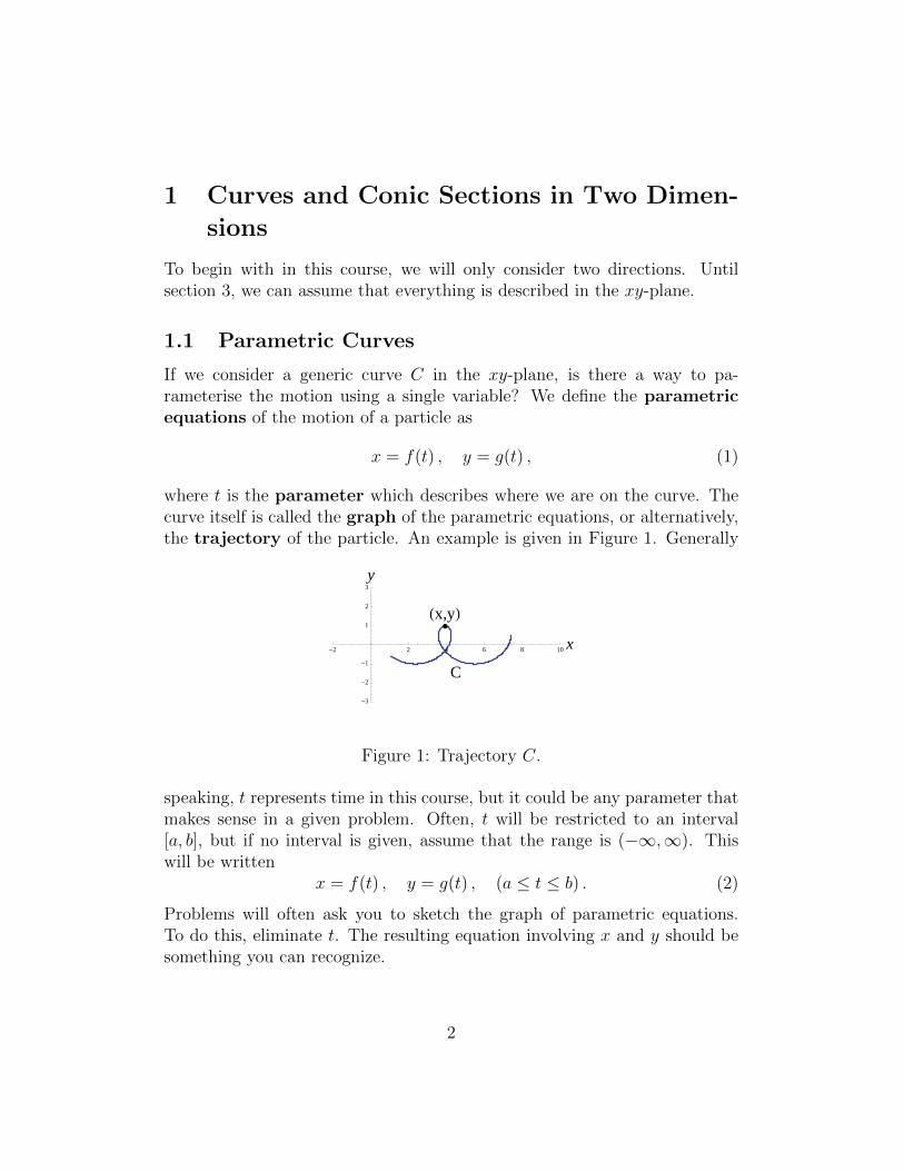
where t is the parameter which describes where we are on the curve. Thecurve itself is called the graph of the parametric equations, or alternatively,the trajectory of the particle. An example is given in Figure 1. Generally

C

Hx,yL

-2 2 4 6 8 10 x

-3

-2

-1

1

2

3

y

Figure 1: Trajectory C.

speaking, t represents time in this course, but it could be any parameter thatmakes sense in a given problem. Often, t will be restricted to an interval[a, b], but if no interval is given, assume that the range is (−∞,∞). Thiswill be written

x = f(t) , y = g(t) , (a ≤ t ≤ b) . (2)

Problems will often ask you to sketch the graph of parametric equations.To do this, eliminate t. The resulting equation involving x and y should besomething you can recognize.

2

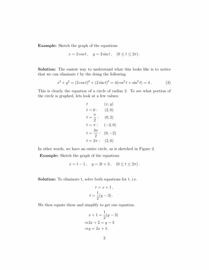
Example: Sketch the graph of the equations

x = 2 cos t , y = 2 sin t , (0 ≤ t ≤ 2π) .

Solution: The easiest way to understand what this looks like is to noticethat we can eliminate t by the doing the following

x2 + y2 = (2 cos t)2 + (2 sin t)2 = 4(cos2 t+ sin2 t) = 4 . (3)

This is clearly the equation of a circle of radius 2. To see what portion ofthe circle is graphed, lets look at a few values:

t (x, y)

t = 0 : (2, 0)

t =π

2: (0, 2)

t = π : (−2, 0)

t =3π

2: (0,−2)

t = 2π : (2, 0)

In other words, we have an entire circle, as is sketched in Figure 2.

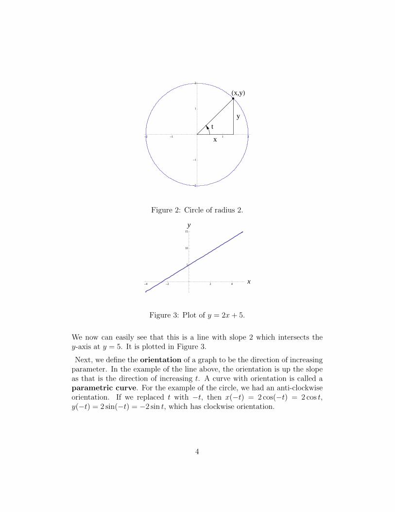
Example: Sketch the graph of the equations

x = t− 1 , y = 2t+ 3 , (0 ≤ t ≤ 2π) .

Solution: To eliminate t, solve both equations for t, i.e.

t = x+ 1 ,

t =1

2(y − 3) .

We then equate these and simplify to get one equation.

x+ 1 =1

2(y − 3)

⇒2x+ 2 = y − 3

⇒y = 2x+ 5 .

3

y

x

Hx,yL

t

-2 -1 1 2

-2

-1

1

2

Figure 2: Circle of radius 2.

-4 -2 2 4x

5

10

15

y

Figure 3: Plot of y = 2x+ 5.

We now can easily see that this is a line with slope 2 which intersects they-axis at y = 5. It is plotted in Figure 3.

Next, we define the orientation of a graph to be the direction of increasingparameter. In the example of the line above, the orientation is up the slopeas that is the direction of increasing t. A curve with orientation is called aparametric curve. For the example of the circle, we had an anti-clockwiseorientation. If we replaced t with −t, then x(−t) = 2 cos(−t) = 2 cos t,y(−t) = 2 sin(−t) = −2 sin t, which has clockwise orientation.

4

1.1.1 Expressing equations parametrically

We can always describe the equation y = f(x) parametrically. The simplestway to do this is to take x = t and then y = f(t).

Example: y = x2 + 1.

Solution: x = t⇒ y = t2 + 1.

Of course, for something like a circle you can of course do the same. However,there are often better parameterisations to chose. In the case of a circle ofradius a, the parameterisation x = a cos t, y = a sin t is often convenient.

1.1.2 Tangent lines for parametric curves

Recall that the tangent line to a curve y = f(x) at a point P is the line

that passes through P that has slope m = df(x)dt

. For a parametric curve, wecan find the slope using the parameter t via the chain rule:

dy

dx=dy/dt

dx/dt. (4)

There are three special types of tangent lines:

• If dy/dt = 0 and dx/dt 6= 0, the slope is 0 and we have a horizontaltangent line.

• If dx/dt = 0 and dy/dt 6= 0, the slope is infinite and we have a verticaltangent line.

• If dx/dt = 0 and dy/dt = 0, the slope is indeterminate and we have asingular point. These require special treatment.

Let’s look at an example.

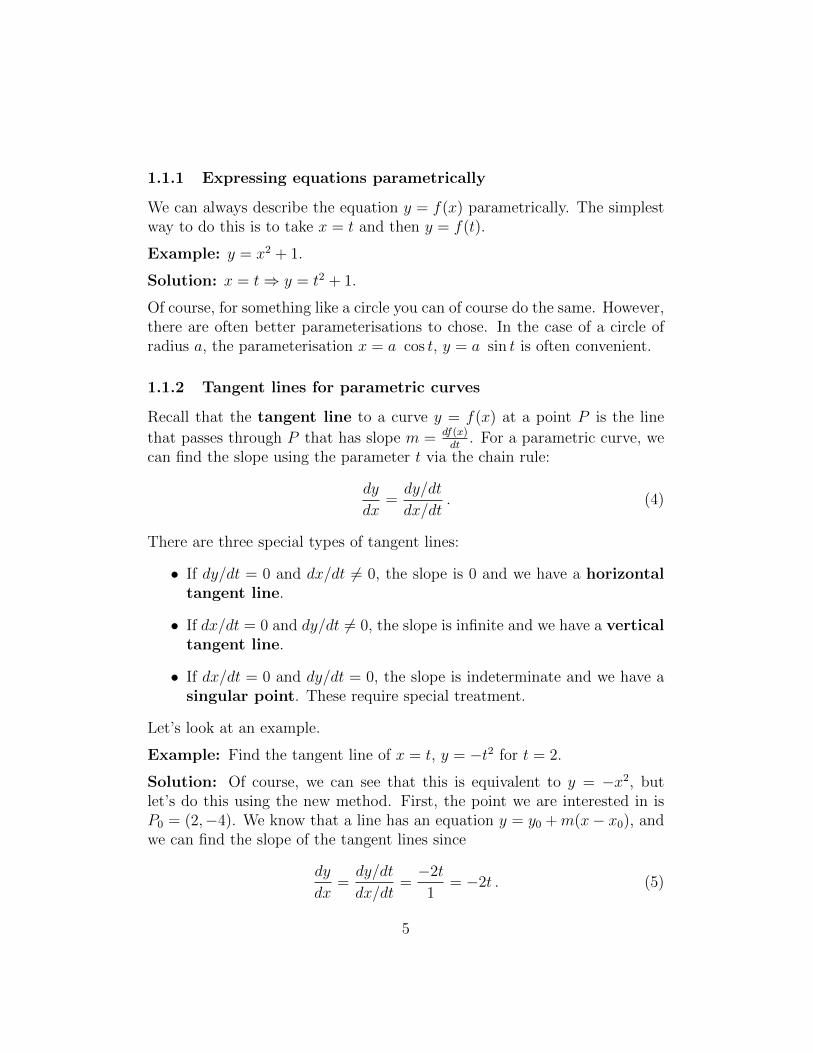
Example: Find the tangent line of x = t, y = −t2 for t = 2.

Solution: Of course, we can see that this is equivalent to y = −x2, butlet’s do this using the new method. First, the point we are interested in isP0 = (2,−4). We know that a line has an equation y = y0 +m(x− x0), andwe can find the slope of the tangent lines since

dy

dx=dy/dt

dx/dt=−2t

1= −2t . (5)

5

Therefore, at P0

m|P0 = −2(2) = −4 . (6)

The equation of the tangent line is then

y = −4− 4(x− 2) = 4− 4x . (7)

This is sketched in Figure 4.

H2,-4L-4 -2 2 4 x

-15

-10

-5

y

Figure 4: Tangent line to the function y = −x2.

1.1.3 Arc Length of a Parametric Curve

For a parametric curve

x = x(t) , y = y(t) , (a ≤ t ≤ b) , (8)

the arc length is given by

L =

∫ b

a

√(dx

dt

)2

+

(dy

dt

)2

dt . (9)

Example: Find the circumference of the circle

x = a cos t , y = a sin t , (0 ≤ t ≤ 2π) .

6

Solution: We find

L =

∫ 2π

0

√(−a sin t)2 + (a cos t)2 dt =

∫ 2π

0

at dt = 2πa .

If the curve doubles over, this will not work: in other words no point on thecurve should be graphed by two values of t. In our example of the circle, ifwe integrated from 0 to 3π we would find 3πa, which is obviously not thecircumference, because the values between 2π and 3π repeat those between0 and π.

1.2 Polar Coordinates

Up until now we have been dealing with the coordinates x and y, which areknown as Cartesian coordinates or rectangular coordinates. We canequally describe a plane using any pair of coordinates so that each positionon the plane is uniquely described by the pair. In particular a useful set ofcoordinates are polar coordinates.

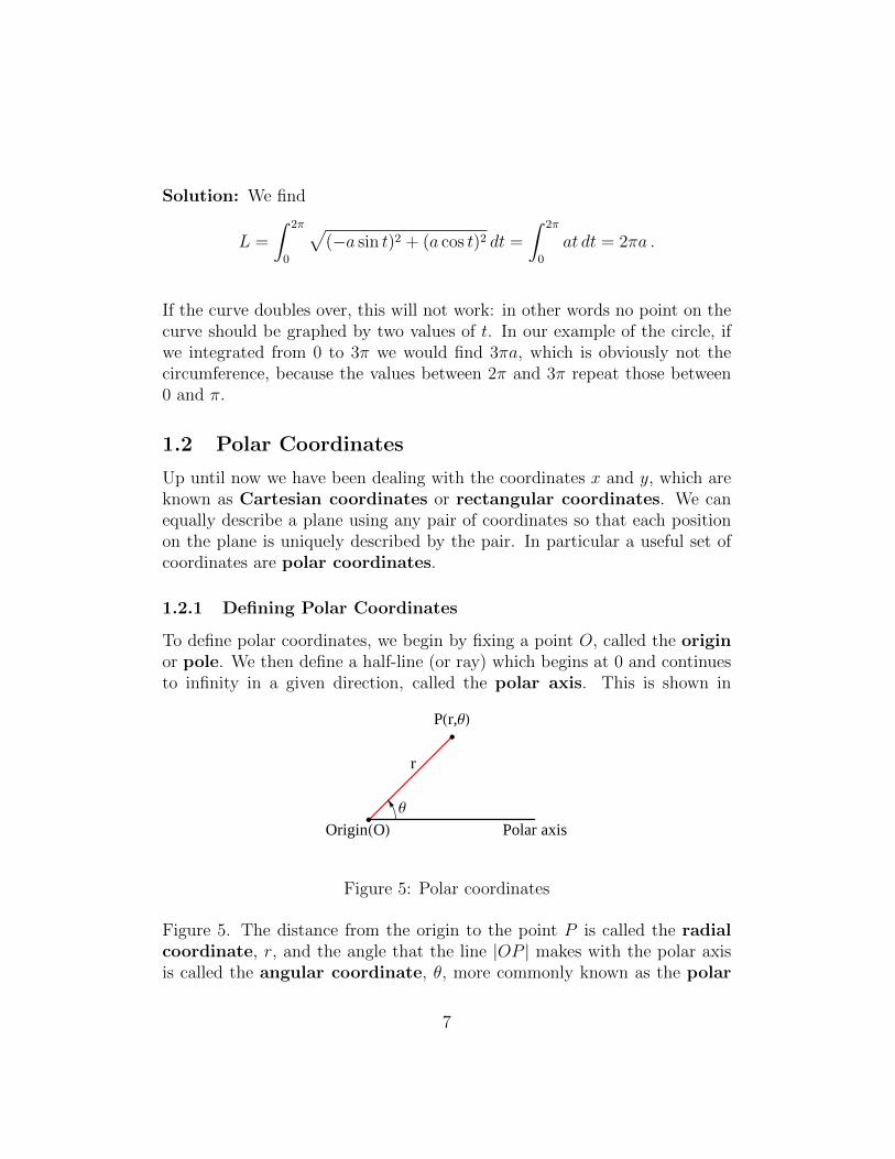
1.2.1 Defining Polar Coordinates

To define polar coordinates, we begin by fixing a point O, called the originor pole. We then define a half-line (or ray) which begins at 0 and continuesto infinity in a given direction, called the polar axis. This is shown in

Θ

r

PHr,ΘL

OriginHOL Polar axis

Figure 5: Polar coordinates

Figure 5. The distance from the origin to the point P is called the radialcoordinate, r, and the angle that the line |OP | makes with the polar axisis called the angular coordinate, θ, more commonly known as the polar

7

angle. It is important to notice that the polar angle returns to its originalposition when the angle is 2π. Therefore, any angle greater than or equalto 2π is equivalent to an angle in the range (0 ≤ θ ≤ 2π). In fact, moregenerally, the angles θ−2π n, θ and θ+ 2π n are equivalent if n is an integer.

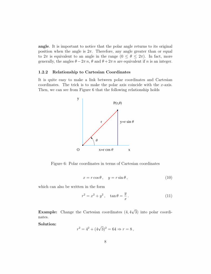
1.2.2 Relationship to Cartesian Coordinates

It is quite easy to make a link between polar coordinates and Cartesiancoordinates. The trick is to make the polar axis coincide with the x-axis.Then, we can see from Figure 6 that the following relationship holds

Θ

r

PHr,ΘL

O x

y

x=r cos Θ

y=r sin Θ

Figure 6: Polar coordinates in terms of Cartesian coordinates

x = r cos θ , y = r sin θ , (10)

which can also be written in the form

r2 = x2 + y2 , tan θ =y

x. (11)

Example: Change the Cartesian coordinates (4, 4√

3) into polar coordi-nates.

Solution:r2 = 42 + (4

√3)2 = 64⇒ r = 8 ,

8

and

tan θ =4√

3

4=√

3⇒ θ =π

3.

The polar coordinates are therefore (r, θ) = (8, π/3).

Example: Change the polar coordinates (3, 3π/4) into Cartesian coordi-nates.

Solution:

x = 3 cos3π

4= − 3√

2,

and

y = 3 sin3π

4=

3√2,

The Cartesian coordinates are therefore (x, y) = (−3/√

2, 3/√

2).

If you are asked to graph an equation in polar coordinates, the easiest thing

Π�2

0

Π

3Π�2

Π�4

-1.0 -0.5 0.5 1.0

-1.0

-0.5

0.5

1.0

r=0

1

2

3

-1 1 2 3 4

-1

1

2

3

4

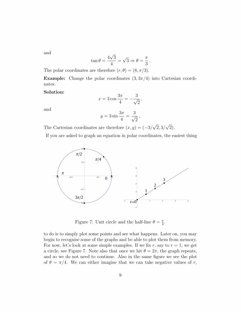
Figure 7: Unit circle and the half-line θ = π4.

to do is to simply plot some points and see what happens. Later on, you maybegin to recognise some of the graphs and be able to plot them from memory.For now, let’s look at some simple examples. If we fix r, say to r = 1, we geta circle, see Figure 7. Note also that once we hit θ = 2π, the graph repeats,and so we do not need to continue. Also in the same figure we see the plotof θ = π/4. We can either imagine that we can take negative values of r,

9

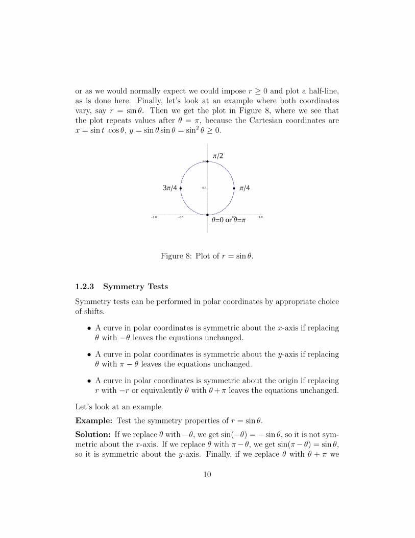
or as we would normally expect we could impose r ≥ 0 and plot a half-line,as is done here. Finally, let’s look at an example where both coordinatesvary, say r = sin θ. Then we get the plot in Figure 8, where we see thatthe plot repeats values after θ = π, because the Cartesian coordinates arex = sin t cos θ, y = sin θ sin θ = sin2 θ ≥ 0.

Π�2

Θ=0 or Θ=Π

Π�43Π�4

-1.0 -0.5 0.5 1.0

0.5

1.0

Figure 8: Plot of r = sin θ.

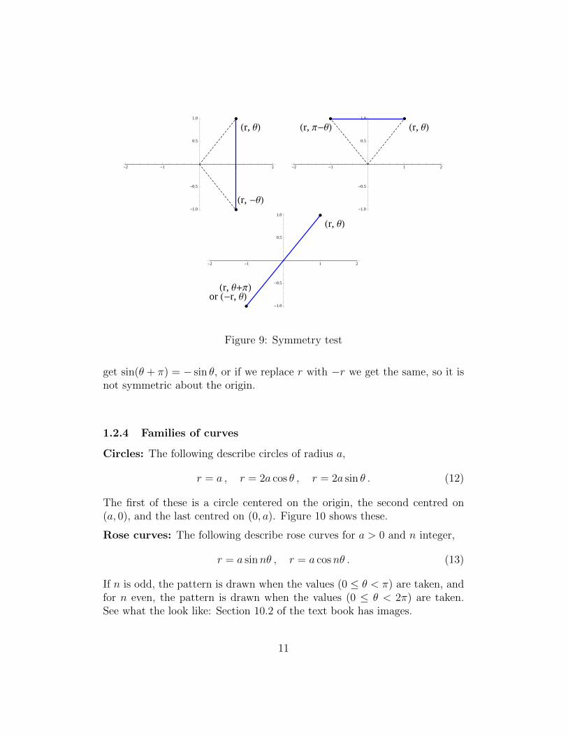
1.2.3 Symmetry Tests

Symmetry tests can be performed in polar coordinates by appropriate choiceof shifts.

• A curve in polar coordinates is symmetric about the x-axis if replacingθ with −θ leaves the equations unchanged.

• A curve in polar coordinates is symmetric about the y-axis if replacingθ with π − θ leaves the equations unchanged.

• A curve in polar coordinates is symmetric about the origin if replacingr with −r or equivalently θ with θ+π leaves the equations unchanged.

Let’s look at an example.

Example: Test the symmetry properties of r = sin θ.

Solution: If we replace θ with −θ, we get sin(−θ) = − sin θ, so it is not sym-metric about the x-axis. If we replace θ with π− θ, we get sin(π− θ) = sin θ,so it is symmetric about the y-axis. Finally, if we replace θ with θ + π we

10

Hr, ΘL

Hr, -ΘL

-2 -1 1 2

-1.0

-0.5

0.5

1.0

Hr, ΘLHr, Π-ΘL

-2 -1 1 2

-1.0

-0.5

0.5

1.0

Hr, ΘL

Hr, Θ+ΠLor H-r, ΘL

-2 -1 1 2

-1.0

-0.5

0.5

1.0

Figure 9: Symmetry test

get sin(θ + π) = − sin θ, or if we replace r with −r we get the same, so it isnot symmetric about the origin.

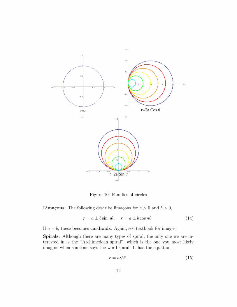
1.2.4 Families of curves

Circles: The following describe circles of radius a,

r = a , r = 2a cos θ , r = 2a sin θ . (12)

The first of these is a circle centered on the origin, the second centred on(a, 0), and the last centred on (0, a). Figure 10 shows these.

Rose curves: The following describe rose curves for a > 0 and n integer,

r = a sinnθ , r = a cosnθ . (13)

If n is odd, the pattern is drawn when the values (0 ≤ θ < π) are taken, andfor n even, the pattern is drawn when the values (0 ≤ θ < 2π) are taken.See what the look like: Section 10.2 of the text book has images.

11

r=a

-1.5 -1.0 -0.5 0.5 1.0 1.5

-1.5

-1.0

-0.5

0.5

1.0

1.5

r=2a Cos Θ

0.5 1.0 1.5 2.0 2.5

-1.5

-1.0

-0.5

0.5

1.0

1.5

r=2a Sin Θ-1.5 -1.0 -0.5 0.5 1.0 1.5

-0.5

0.5

1.0

1.5

2.0

2.5

Figure 10: Families of circles

Limacons: The following describe limacons for a > 0 and b > 0,

r = a± b sinnθ , r = a± b cosnθ . (14)

If a = b, these becomes cardioids. Again, see textbook for images.

Spirals: Although there are many types of spiral, the only one we are in-terested in is the “Archimedean spiral”, which is the one you most likelyimagine when someone says the word spiral. It has the equation

r = a√θ . (15)

12

1.2.5 Tangent Lines in Polar Coordinates

If we take a general curve of the form r = f(θ) and write it in terms of its xand y coordinates, we would have

x = f(θ) cos θ , y = f(θ) sin θ . (16)

This is now a parametric curve in parameter θ, and so we can find the slopeof the tangent line provided f(θ) is differentiable. We have

dx

dθ= −f(θ) sin θ + f ′(θ) cos θ = −r sin θ +

dr

dθcos θ ,

dy

dθ= f(θ) cos θ + f ′(θ) sin θ = r cos θ +

dr

dθsin θ ,

(17)

and the slope isdy

dx=

dydθdxdθ

=r cos θ + dr

dθsin θ

−r sin θ + drdθ

cos θ. (18)

Example: Find the slope of the tangent line to the circle r = 2 cos θ atθ = π/3.

Solution: We get drdθ

= −2 sin θ, and so

dy

dx=

2 cos2 θ − 2 sin2 θ

−2 sin θ cos θ − 2 sin θ cos θ=

2 cos 2θ

−2 sin 2θ= − cot 2θ .

Therefore, the slope at θ = π/3 is

m = − cot2π

3=

1√3.

1.2.6 Tangent Lines to Polar Curves at the Origin

At the origin, we have r = 0 with angle θ0, so assuming that drdθ6= 0 at the

origin, the equation becomes

dy

dx=

0 + drdθ

sin θ0

0 + drdθ

cos θ0

= tan θ0 . (19)

The line with this slope is the line θ = θ0, and so this line is tangent to thecurve at the origin. To recall what this line looks like, return to section 1.2.2.

13

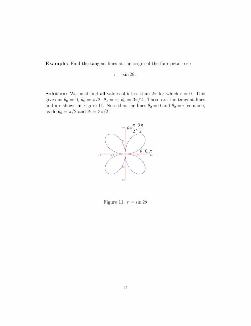
Example: Find the tangent lines at the origin of the four-petal rose

r = sin 2θ .

Solution: We must find all values of θ less than 2π for which r = 0. Thisgives us θ0 = 0, θ0 = π/2, θ0 = π, θ0 = 3π/2. These are the tangent linesand are shown in Figure 11. Note that the lines θ0 = 0 and θ0 = π coincide,as do θ0 = π/2 and θ0 = 3π/2.

Θ=0, Π

Θ=Π

2,3 Π

2

-1.0 -0.5 0.5 1.0

-1.0

-0.5

0.5

1.0

Figure 11: r = sin 2θ

14

1.2.7 Arc Length in Polar Coordinates

To find the arc length in terms of polar coordinates, we recall formula (9)and substitute the results of (17), giving(

dx

dθ

)2

+

(dy

dθ

)2

=

(−r sin θ +

dr

dθcos θ

)2

+

(r cos θ +

dr

dθsin θ

)2

= r2(sin2 θ + cos2 θ) + 2rdr

dθcos θ sin θ

− 2rdr

dθcos θ sin θ +

(dr

dθ

)2

(sin2 θ + cos2 θ)

= r2 +

(dr

dθ

)2

,

(20)

which results in

L =

∫ β

α

√r2 +

(dr

dθ

)2

dθ (21)

Let’s look at an example.

Example: Find the arc length of the logarithmic spiral r = aebθ betweenθ = 0 and θ = π.

Solution:

L =

∫ π

0

√(aebθ)2 + (abebθ)2dθ

=

∫ π

0

a√

1 + b2ebθdθ =a

b

√1 + b2ebθ

∣∣π0

=a

b

√1 + b2(ebπ − 1) .

(22)

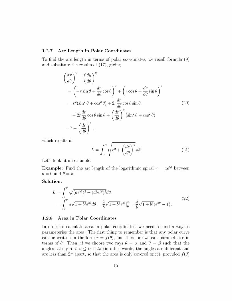
1.2.8 Area in Polar Coordinates

In order to calculate area in polar coordinates, we need to find a way toparameterise the area. The first thing to remember is that any polar curvecan be written in the form r = f(θ), and therefore we can parameterise interms of θ. Then, if we choose two rays θ = α and θ = β such that theangles satisfy α < β ≤ α + 2π (in other words, the angles are different andare less than 2π apart, so that the area is only covered once), provided f(θ)

15

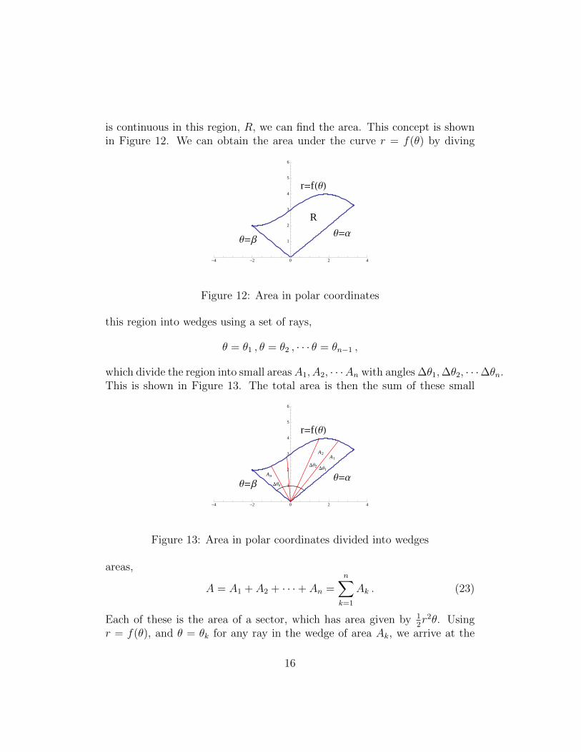
is continuous in this region, R, we can find the area. This concept is shownin Figure 12. We can obtain the area under the curve r = f(θ) by diving

r=fHΘL

Θ=ΒΘ=Α

R

-4 -2 0 2 4

1

2

3

4

5

6

Figure 12: Area in polar coordinates

this region into wedges using a set of rays,

θ = θ1 , θ = θ2 , · · · θ = θn−1 ,

which divide the region into small areasA1, A2, · · ·An with angles ∆θ1,∆θ2, · · ·∆θn.This is shown in Figure 13. The total area is then the sum of these small

r=fHΘL

Θ=ΒΘ=Α

DΘn

DΘ2 DΘ1

An

A2A1

-4 -2 0 2 4

1

2

3

4

5

6

Figure 13: Area in polar coordinates divided into wedges

areas,

A = A1 + A2 + · · ·+ An =n∑k=1

Ak . (23)

Each of these is the area of a sector, which has area given by 12r2θ. Using

r = f(θ), and θ = θk for any ray in the wedge of area Ak, we arrive at the

16

discrete version of the area formula

A =n∑k=1

Ak ∼n∑k=1

1

2[f(θk)]

2∆θk . (24)

We can take the limit where these angles ∆θk vanish to give an integral form

A = lim∆k→0

n∑k=1

1

2[f(θk)]

2∆θk =

∫ β

α

1

2[f(θ)]2 dθ . (25)

Thus, the area of a region R under a continuous curve r = f(θ) and betweenθ = α and θ = β is

A =

∫ β

α

1

2[f(θ)]2 dθ =

∫ β

α

1

2r2 dθ . (26)

The most difficult parts of this is generally finding the limits of integration.Sometimes you will be told explicitly.Important note: Always draw the region to help you identify the limits.

Let’s look at a simple example.

Example: Find the area of the circle r = 2a sin θ.

Solution: This looks like the third types of circle Figure 10. Since we wantthe area of the whole circle, the limits are 0 ≤ θ ≤ π since the entire circleis above the x-axis. Note that for a circle centered on the origin r = a, thelimits would be 0 ≤ θ ≤ 2π. The area is

A =

∫ π

0

1

2(2a sin θ)2 dθ = 2a2

∫ π

0

sin2 θ dθ

= 2a2

∫ π

0

1

2(1− cos 2θ) dθ = 2a2

(1

2θ∣∣π0− 0

)= πa2 .

We can often make use of the symmetry of the region to simplify a problem.For example, the upper and lower semi-circles of a full circle are mirror imagesand obviously have the same area. Hence∫ 2π

0

1

2a2 dθ = 2

∫ π

0

1

2a2 = πa2 , (27)

17

is clearly true. Let’s look at a more complicated example to help understandthis.

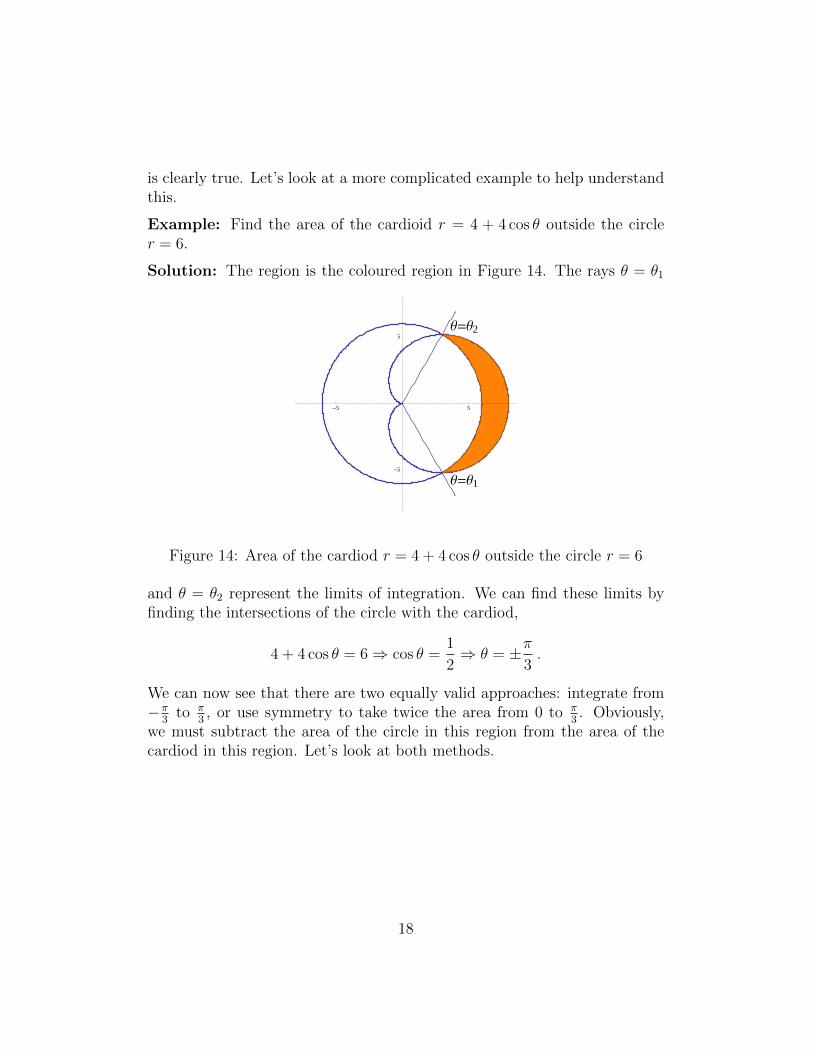
Example: Find the area of the cardioid r = 4 + 4 cos θ outside the circler = 6.

Solution: The region is the coloured region in Figure 14. The rays θ = θ1

Θ=Θ2

Θ=Θ1

-5 5

-5

5

Figure 14: Area of the cardiod r = 4 + 4 cos θ outside the circle r = 6

and θ = θ2 represent the limits of integration. We can find these limits byfinding the intersections of the circle with the cardiod,

4 + 4 cos θ = 6⇒ cos θ =1

2⇒ θ = ±π

3.

We can now see that there are two equally valid approaches: integrate from−π

3to π

3, or use symmetry to take twice the area from 0 to π

3. Obviously,

we must subtract the area of the circle in this region from the area of thecardiod in this region. Let’s look at both methods.

18

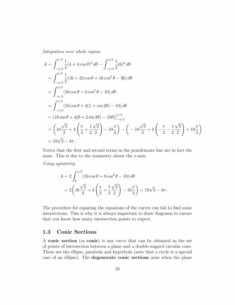
Integration over whole region:

A =

∫ π/3

−π/3

1

2(4 + 4 cos θ)2 dθ −

∫ π/3

−π/3

1

2(6)2 dθ

=

∫ π/3

−π/3

1

2(16 + 32 cos θ + 16 cos2 θ − 36) dθ

=

∫ π/3

−π/3(16 cos θ + 8 cos2 θ − 10) dθ

=

∫ π/3

−π/3(16 cos θ + 4(1 + cos 2θ)− 10) dθ

= (16 sin θ + 4(θ + 2 sin 2θ)− 10θ)∣∣π/3−π/3

=

(16

√3

2+ 4

(π

3+

1

2

√3

2

)− 10

π

3

)−(− 16

√3

2+ 4

(−π

3− 1

2

√3

2

)+ 10

π

3

)= 18

√3− 4π .

Notice that the first and second terms in the penultimate line are in fact thesame. This is due to the symmetry about the x-axis.

Using symmetry:

A = 2

∫ π/3

0

(16 cos θ + 8 cos2 θ − 10) dθ

= 2

(16

√3

2+ 4

(π

3+

1

2

√3

2

)− 10

π

3

)= 18

√3− 4π .

The procedure for equating the equations of the curves can fail to find someintersections. This is why it is always important to draw diagrams to ensurethat you know how many intersection points to expect.

1.3 Conic Sections

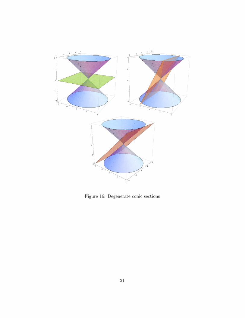
A conic section (or conic) is any curve that can be obtained as the setof points of intersection between a plane and a double-napped circular cone.These are the ellipse, parabola and hyperbola (note that a circle is a specialcase of an ellipse). The degenerate conic sections arise when the plane

19

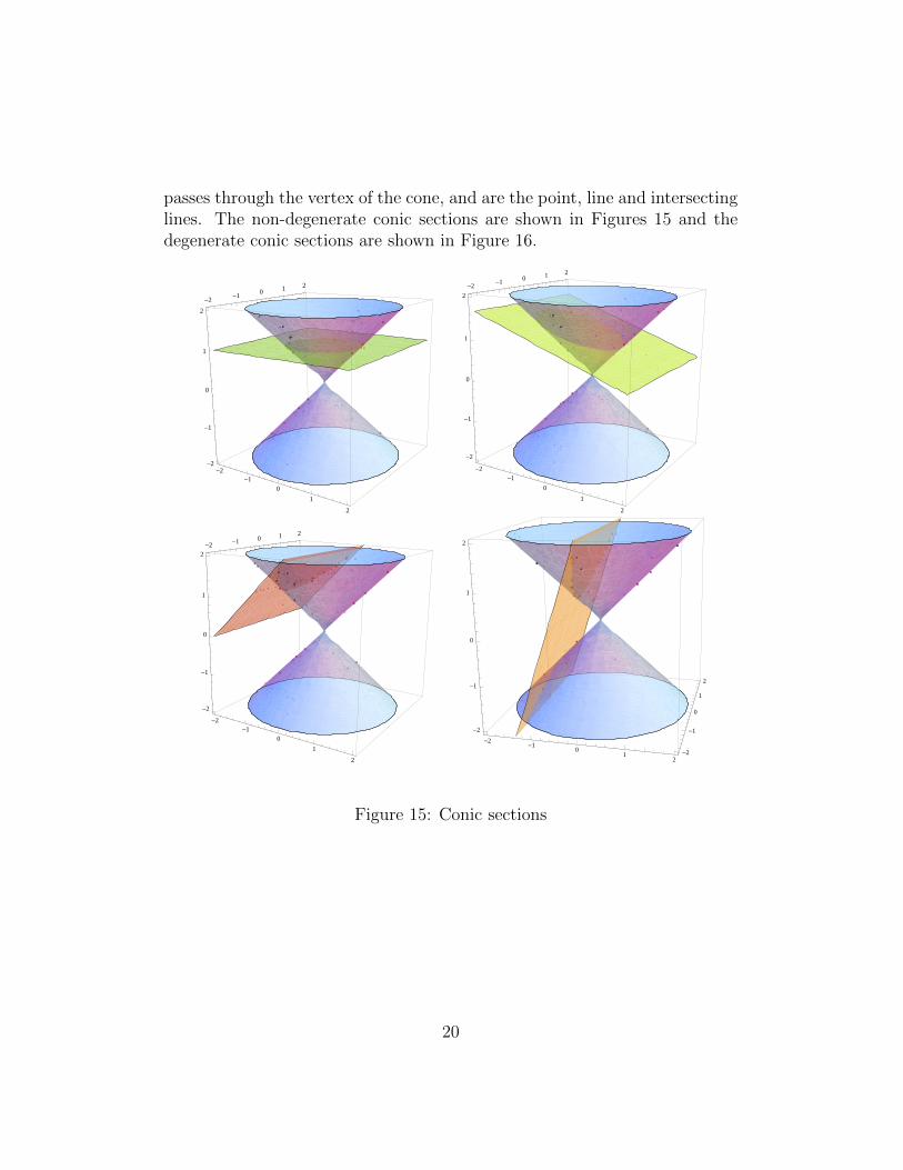
passes through the vertex of the cone, and are the point, line and intersectinglines. The non-degenerate conic sections are shown in Figures 15 and thedegenerate conic sections are shown in Figure 16.

-2

-1

0

1

2

-2-1

01

2

-2

-1

0

1

2

-2

-1

0

1

2

-2-1

01

2

-2

-1

0

1

2

-2

-1

0

1

2

-2-1

01

2

-2

-1

0

1

2

-2-1

01

2

-2

-1

0

1

2

-2

-1

0

1

2

Figure 15: Conic sections

20

-2

-1

0

1

2

-2-1

01

2

-2

-1

0

1

2

-2

-1

0

1

2

-2-1

01

2

-2

-1

0

1

2

-2

-1

0

1

2-2

-1

0

1

2

-2

-1

0

1

2

Figure 16: Degenerate conic sections

21

1.3.1 Types of Conic Section

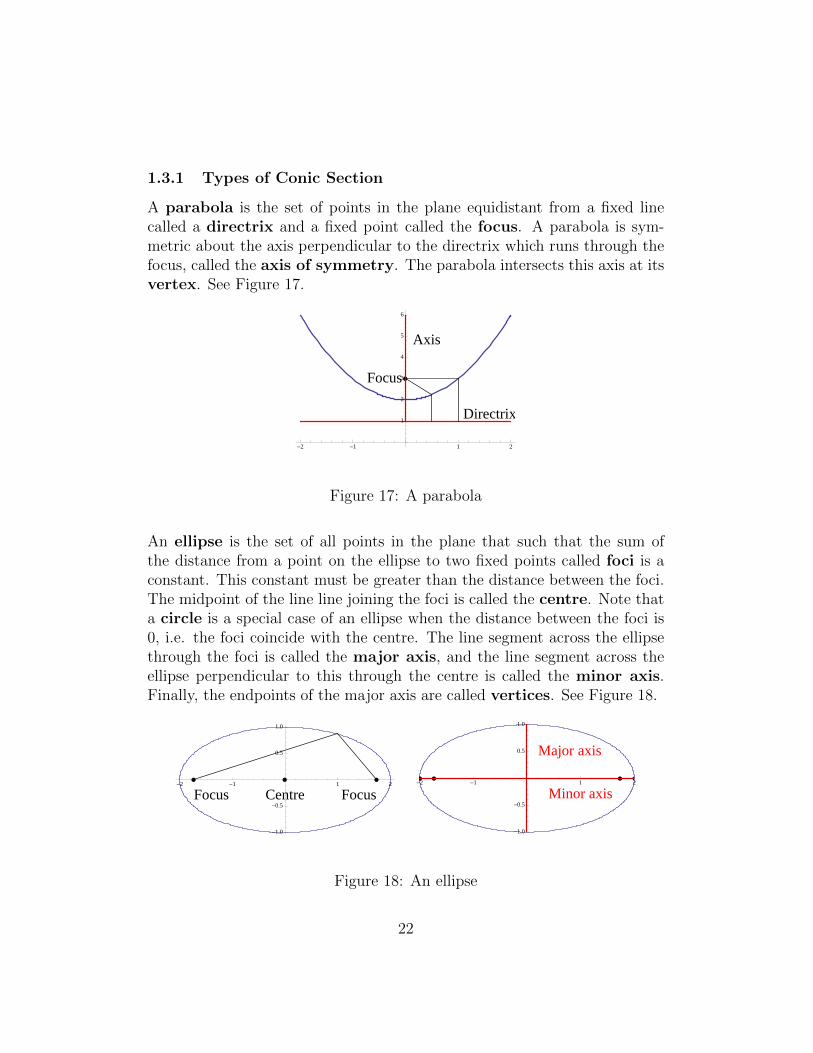
A parabola is the set of points in the plane equidistant from a fixed linecalled a directrix and a fixed point called the focus. A parabola is sym-metric about the axis perpendicular to the directrix which runs through thefocus, called the axis of symmetry. The parabola intersects this axis at itsvertex. See Figure 17.

Directrix

Axis

Focus

-2 -1 1 2

1

2

3

4

5

6

Figure 17: A parabola

An ellipse is the set of all points in the plane that such that the sum ofthe distance from a point on the ellipse to two fixed points called foci is aconstant. This constant must be greater than the distance between the foci.The midpoint of the line line joining the foci is called the centre. Note thata circle is a special case of an ellipse when the distance between the foci is0, i.e. the foci coincide with the centre. The line segment across the ellipsethrough the foci is called the major axis, and the line segment across theellipse perpendicular to this through the centre is called the minor axis.Finally, the endpoints of the major axis are called vertices. See Figure 18.

FocusFocus Centre-2 -1 1 2

-1.0

-0.5

0.5

1.0

Minor axis

Major axis

-2 -1 1 2

-1.0

-0.5

0.5

1.0

Figure 18: An ellipse

22

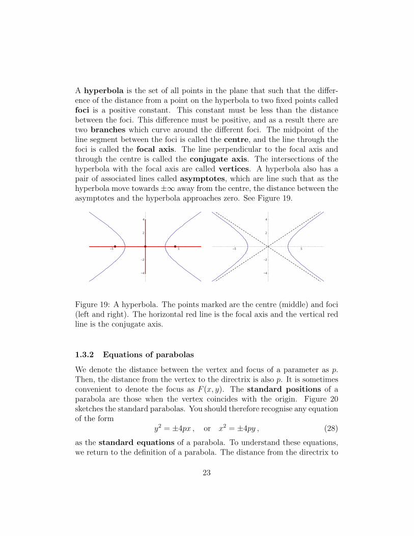
A hyperbola is the set of all points in the plane that such that the differ-ence of the distance from a point on the hyperbola to two fixed points calledfoci is a positive constant. This constant must be less than the distancebetween the foci. This difference must be positive, and as a result there aretwo branches which curve around the different foci. The midpoint of theline segment between the foci is called the centre, and the line through thefoci is called the focal axis. The line perpendicular to the focal axis andthrough the centre is called the conjugate axis. The intersections of thehyperbola with the focal axis are called vertices. A hyperbola also has apair of associated lines called asymptotes, which are line such that as thehyperbola move towards ±∞ away from the centre, the distance between theasymptotes and the hyperbola approaches zero. See Figure 19.

-5 5

-4

-2

2

4

-5 5

-4

-2

2

4

Figure 19: A hyperbola. The points marked are the centre (middle) and foci(left and right). The horizontal red line is the focal axis and the vertical redline is the conjugate axis.

1.3.2 Equations of parabolas

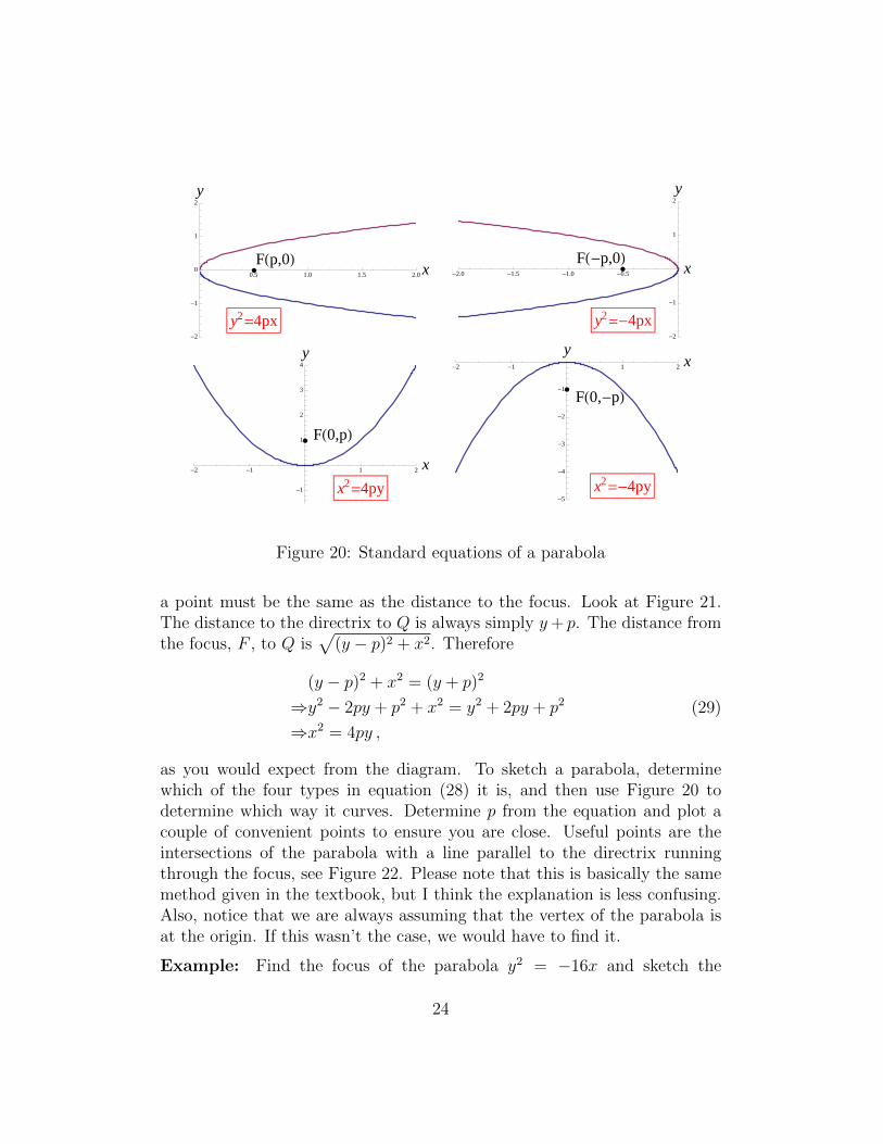
We denote the distance between the vertex and focus of a parameter as p.Then, the distance from the vertex to the directrix is also p. It is sometimesconvenient to denote the focus as F (x, y). The standard positions of aparabola are those when the vertex coincides with the origin. Figure 20sketches the standard parabolas. You should therefore recognise any equationof the form

y2 = ±4px , or x2 = ±4py , (28)

as the standard equations of a parabola. To understand these equations,we return to the definition of a parabola. The distance from the directrix to

23

FHp,0L

y2=4px

0.5 1.0 1.5 2.0 x

-2

-1

0

1

2

y

FH-p,0L

y2=-4px

-2.0 -1.5 -1.0 -0.5 x

-2

-1

1

2

y

FH0,pL

x2=4py

-2 -1 1 2 x

-1

1

2

3

4

y

FH0,-pL

x2=-4py

-2 -1 1 2 x

-5

-4

-3

-2

-1

y

Figure 20: Standard equations of a parabola

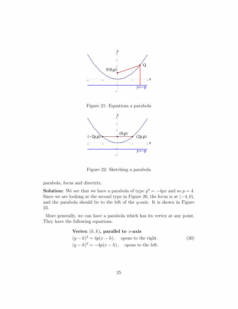
a point must be the same as the distance to the focus. Look at Figure 21.The distance to the directrix to Q is always simply y+ p. The distance fromthe focus, F , to Q is

√(y − p)2 + x2. Therefore

(y − p)2 + x2 = (y + p)2

⇒y2 − 2py + p2 + x2 = y2 + 2py + p2

⇒x2 = 4py ,

(29)

as you would expect from the diagram. To sketch a parabola, determinewhich of the four types in equation (28) it is, and then use Figure 20 todetermine which way it curves. Determine p from the equation and plot acouple of convenient points to ensure you are close. Useful points are theintersections of the parabola with a line parallel to the directrix runningthrough the focus, see Figure 22. Please note that this is basically the samemethod given in the textbook, but I think the explanation is less confusing.Also, notice that we are always assuming that the vertex of the parabola isat the origin. If this wasn’t the case, we would have to find it.

Example: Find the focus of the parabola y2 = −16x and sketch the

24

FH0,pLQ

y=-p

-2 -1 1 2 x

-2

-1

1

2

3

4

y

Figure 21: Equations a parabola

H0,pL H2p,pLH-2p,pL

y=-p

-2 -1 1 2 x

-2

-1

1

2

3

4

y

Figure 22: Sketching a parabola

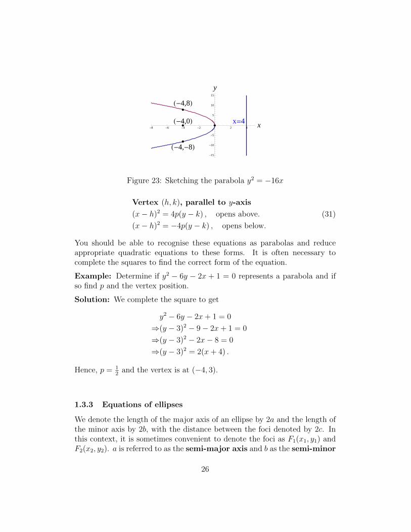
parabola, focus and directrix.

Solution: We see that we have a parabola of type y2 = −4px and so p = 4.Since we are looking at the second type in Figure 20, the focus is at (−4, 0),and the parabola should be to the left of the y-axis. It is shown in Figure23.

More generally, we can have a parabola which has its vertex at any point.They have the following equations:

Vertex (h, k), parallel to x-axis

(y − k)2 = 4p(x− h) , opens to the right.

(y − k)2 = −4p(x− h) , opens to the left.

(30)

25

H-4,0L

H-4,8L

H-4,-8L

x=4-8 -6 -4 -2 2 4 x

-15

-10

-5

5

10

15

y

Figure 23: Sketching the parabola y2 = −16x

Vertex (h, k), parallel to y-axis

(x− h)2 = 4p(y − k) , opens above.

(x− h)2 = −4p(y − k) , opens below.

(31)

You should be able to recognise these equations as parabolas and reduceappropriate quadratic equations to these forms. It is often necessary tocomplete the squares to find the correct form of the equation.

Example: Determine if y2 − 6y − 2x + 1 = 0 represents a parabola and ifso find p and the vertex position.

Solution: We complete the square to get

y2 − 6y − 2x+ 1 = 0

⇒(y − 3)2 − 9− 2x+ 1 = 0

⇒(y − 3)2 − 2x− 8 = 0

⇒(y − 3)2 = 2(x+ 4) .

Hence, p = 12

and the vertex is at (−4, 3).

1.3.3 Equations of ellipses

We denote the length of the major axis of an ellipse by 2a and the length ofthe minor axis by 2b, with the distance between the foci denoted by 2c. Inthis context, it is sometimes convenient to denote the foci as F1(x1, y1) andF2(x2, y2). a is referred to as the semi-major axis and b as the semi-minor

26

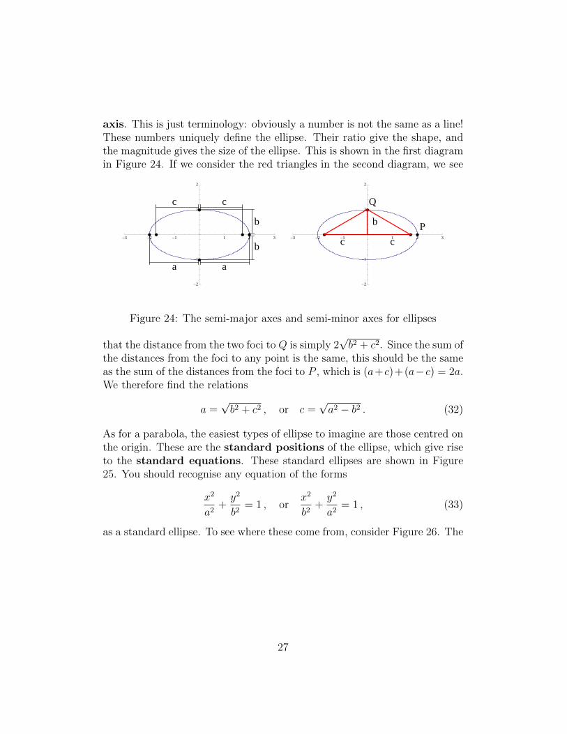
axis. This is just terminology: obviously a number is not the same as a line!These numbers uniquely define the ellipse. Their ratio give the shape, andthe magnitude gives the size of the ellipse. This is shown in the first diagramin Figure 24. If we consider the red triangles in the second diagram, we see

a a

b

b

cc

-3 -2 -1 1 2 3

-2

-1

1

2

b

cc

P

Q

-3 -2 -1 1 2 3

-2

-1

1

2

Figure 24: The semi-major axes and semi-minor axes for ellipses

that the distance from the two foci to Q is simply 2√b2 + c2. Since the sum of

the distances from the foci to any point is the same, this should be the sameas the sum of the distances from the foci to P , which is (a+c)+(a−c) = 2a.We therefore find the relations

a =√b2 + c2 , or c =

√a2 − b2 . (32)

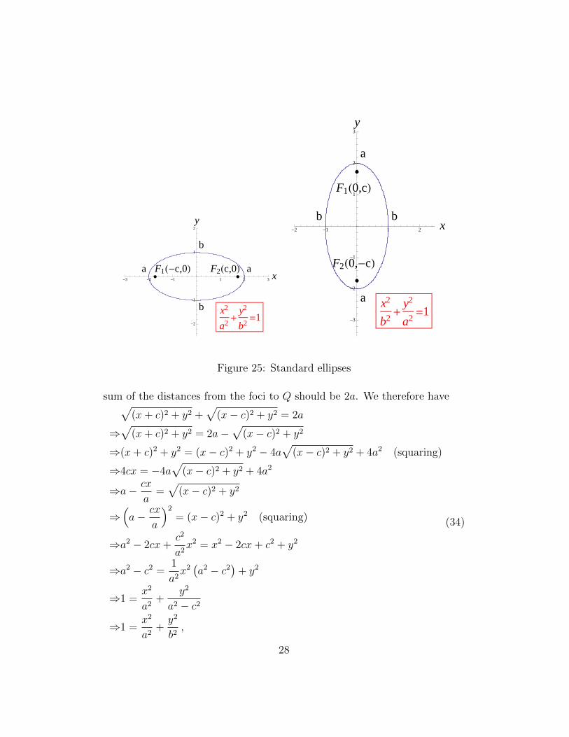
As for a parabola, the easiest types of ellipse to imagine are those centred onthe origin. These are the standard positions of the ellipse, which give riseto the standard equations. These standard ellipses are shown in Figure25. You should recognise any equation of the forms

x2

a2+y2

b2= 1 , or

x2

b2+y2

a2= 1 , (33)

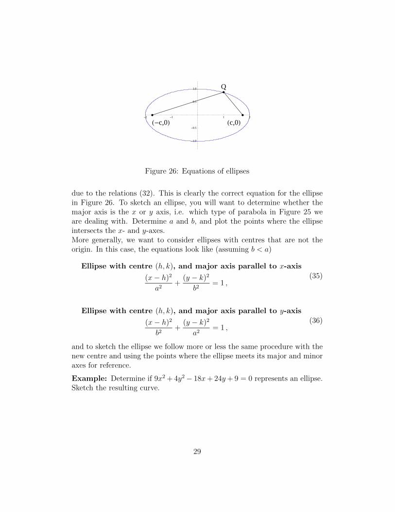
as a standard ellipse. To see where these come from, consider Figure 26. The

27

b

a a

b

F1H-c,0L F2Hc,0L

x2

a2+

y2

b2=1

-3 -2 -1 1 2 3 x

-2

-1

1

2

y

a

b b

a

F2H0,-cL

F1H0,cL

x2

b2+

y2

a2=1

-2 -1 1 2 x

-3

-2

-1

1

2

3

y

Figure 25: Standard ellipses

sum of the distances from the foci to Q should be 2a. We therefore have√(x+ c)2 + y2 +

√(x− c)2 + y2 = 2a

⇒√

(x+ c)2 + y2 = 2a−√

(x− c)2 + y2

⇒(x+ c)2 + y2 = (x− c)2 + y2 − 4a√

(x− c)2 + y2 + 4a2 (squaring)

⇒4cx = −4a√

(x− c)2 + y2 + 4a2

⇒a− cx

a=√

(x− c)2 + y2

⇒(a− cx

a

)2

= (x− c)2 + y2 (squaring)

⇒a2 − 2cx+c2

a2x2 = x2 − 2cx+ c2 + y2

⇒a2 − c2 =1

a2x2(a2 − c2

)+ y2

⇒1 =x2

a2+

y2

a2 − c2

⇒1 =x2

a2+y2

b2,

(34)

28

Hc,0LH-c,0L

Q

-2 -1 1 2

-1.0

-0.5

0.5

1.0

Figure 26: Equations of ellipses

due to the relations (32). This is clearly the correct equation for the ellipsein Figure 26. To sketch an ellipse, you will want to determine whether themajor axis is the x or y axis, i.e. which type of parabola in Figure 25 weare dealing with. Determine a and b, and plot the points where the ellipseintersects the x- and y-axes.More generally, we want to consider ellipses with centres that are not theorigin. In this case, the equations look like (assuming b < a)

Ellipse with centre (h, k), and major axis parallel to x-axis

(x− h)2

a2+

(y − k)2

b2= 1 ,

(35)

Ellipse with centre (h, k), and major axis parallel to y-axis

(x− h)2

b2+

(y − k)2

a2= 1 ,

(36)

and to sketch the ellipse we follow more or less the same procedure with thenew centre and using the points where the ellipse meets its major and minoraxes for reference.

Example: Determine if 9x2 + 4y2− 18x+ 24y+ 9 = 0 represents an ellipse.Sketch the resulting curve.

29

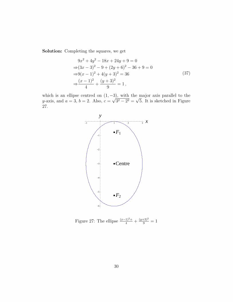
Solution: Completing the squares, we get

9x2 + 4y2 − 18x+ 24y + 9 = 0

⇒(3x− 3)2 − 9 + (2y + 6)2 − 36 + 9 = 0

⇒9(x− 1)2 + 4(y + 3)2 = 36

⇒(x− 1)2

4+

(y + 3)2

9= 1 ,

(37)

which is an ellipse centred on (1,−3), with the major axis parallel to they-axis, and a = 3, b = 2. Also, c =

√32 − 22 =

√5. It is sketched in Figure

27.

F1

F2

Centre

-1 1 2 3 x

-6

-5

-4

-3

-2

-1

y

Figure 27: The ellipse (x−1)2+4

+ (y+3)2

9= 1

30

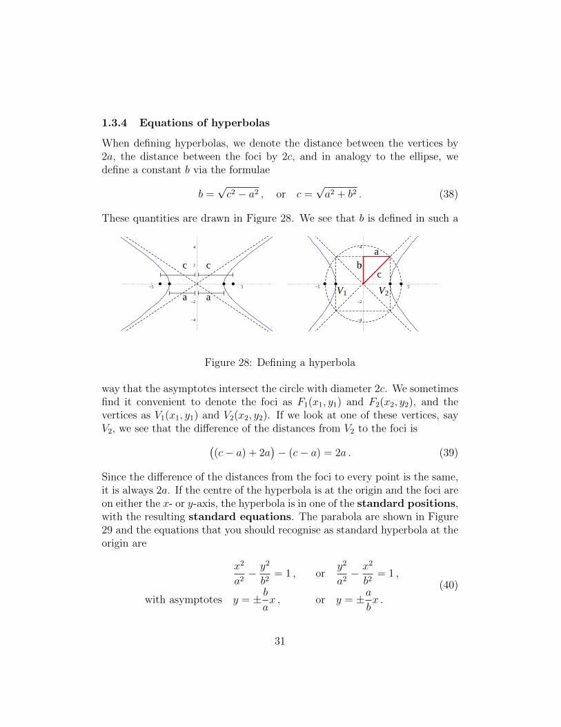
1.3.4 Equations of hyperbolas

When defining hyperbolas, we denote the distance between the vertices by2a, the distance between the foci by 2c, and in analogy to the ellipse, wedefine a constant b via the formulae

b =√c2 − a2 , or c =

√a2 + b2 . (38)

These quantities are drawn in Figure 28. We see that b is defined in such a

aa

c c

-5 5

-4

-2

2

4

a

bc

V1 V2-5 5

-4

-2

2

4

Figure 28: Defining a hyperbola

way that the asymptotes intersect the circle with diameter 2c. We sometimesfind it convenient to denote the foci as F1(x1, y1) and F2(x2, y2), and thevertices as V1(x1, y1) and V2(x2, y2). If we look at one of these vertices, sayV2, we see that the difference of the distances from V2 to the foci is(

(c− a) + 2a)− (c− a) = 2a . (39)

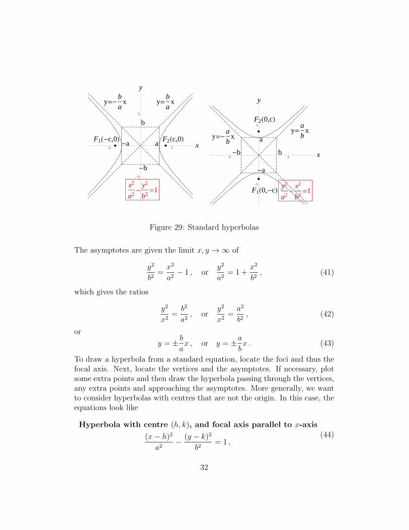
Since the difference of the distances from the foci to every point is the same,it is always 2a. If the centre of the hyperbola is at the origin and the foci areon either the x- or y-axis, the hyperbola is in one of the standard positions,with the resulting standard equations. The parabola are shown in Figure29 and the equations that you should recognise as standard hyperbola at theorigin are

x2

a2− y2

b2= 1 , or

y2

a2− x2

b2= 1 ,

with asymptotes y = ± bax , or y = ±a

bx .

(40)

31

-b

-a a

b

F1H-c,0L F2Hc,0L

y=b

axy=-

b

ax

x2

a2-

y2

b2=1

-5 5 x

-5

5

y

-a

-b b

a

F1H0,-cL

F2H0,cLy=

a

bx

y=-a

bx

y2

a2-

x2

b2=1

-5 5 x

-5

5

y

Figure 29: Standard hyperbolas

The asymptotes are given the limit x, y →∞ of

y2

b2=x2

a2− 1 , or

y2

a2= 1 +

x2

b2, (41)

which gives the ratios

y2

x2=b2

a2, or

y2

x2=a2

b2, (42)

or

y = ± bax , or y = ±a

bx . (43)

To draw a hyperbola from a standard equation, locate the foci and thus thefocal axis. Next, locate the vertices and the asymptotes. If necessary, plotsome extra points and then draw the hyperbola passing through the vertices,any extra points and approaching the asymptotes. More generally, we wantto consider hyperbolas with centres that are not the origin. In this case, theequations look like

Hyperbola with centre (h, k), and focal axis parallel to x-axis

(x− h)2

a2− (y − k)2

b2= 1 ,

(44)

32

Hyperbola with centre (h, k), and focal axis parallel to y-axis

(y − k)2

a2− (x− h)2

b2= 1 ,

(45)

Please note that when we write the hyperbolas this way, the asymptotes forthe first case are the lines with slope ± b

apassing through (h, k) and for the

second first case the asymptotes are the lines with slope ±ab

passing through(h, k).

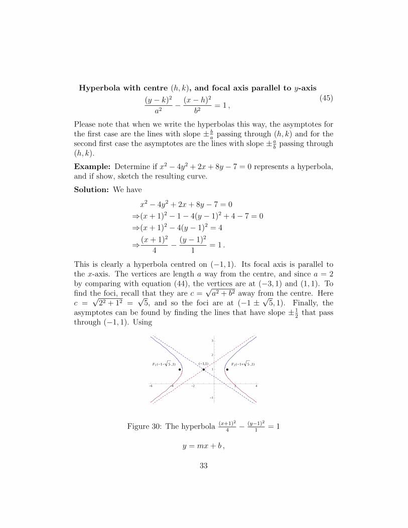
Example: Determine if x2 − 4y2 + 2x+ 8y − 7 = 0 represents a hyperbola,and if show, sketch the resulting curve.

Solution: We have

x2 − 4y2 + 2x+ 8y − 7 = 0

⇒(x+ 1)2 − 1− 4(y − 1)2 + 4− 7 = 0

⇒(x+ 1)2 − 4(y − 1)2 = 4

⇒(x+ 1)2

4− (y − 1)2

1= 1 .

This is clearly a hyperbola centred on (−1, 1). Its focal axis is parallel tothe x-axis. The vertices are length a way from the centre, and since a = 2by comparing with equation (44), the vertices are at (−3, 1) and (1, 1). Tofind the foci, recall that they are c =

√a2 + b2 away from the centre. Here

c =√

22 + 12 =√

5, and so the foci are at (−1 ±√

5, 1). Finally, theasymptotes can be found by finding the lines that have slope ±1

2that pass

through (−1, 1). Using

F1 H-1- 5 ,1L F2 H-1+ 5 ,1LH-1,1L

-6 -4 -2 2 4

-1

1

2

3

Figure 30: The hyperbola (x+1)2

4− (y−1)2

1= 1

y = mx+ b ,

33

we find that for m = 12, b = 3

2and for m = −1

2, b = 1

2. Therefore the

asymptotes are

y =x

2+

3

2, y = −x

2+

1

2.

This parabola is shown in Figure 30.

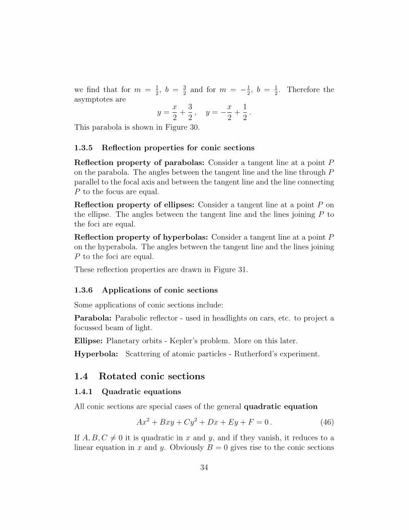
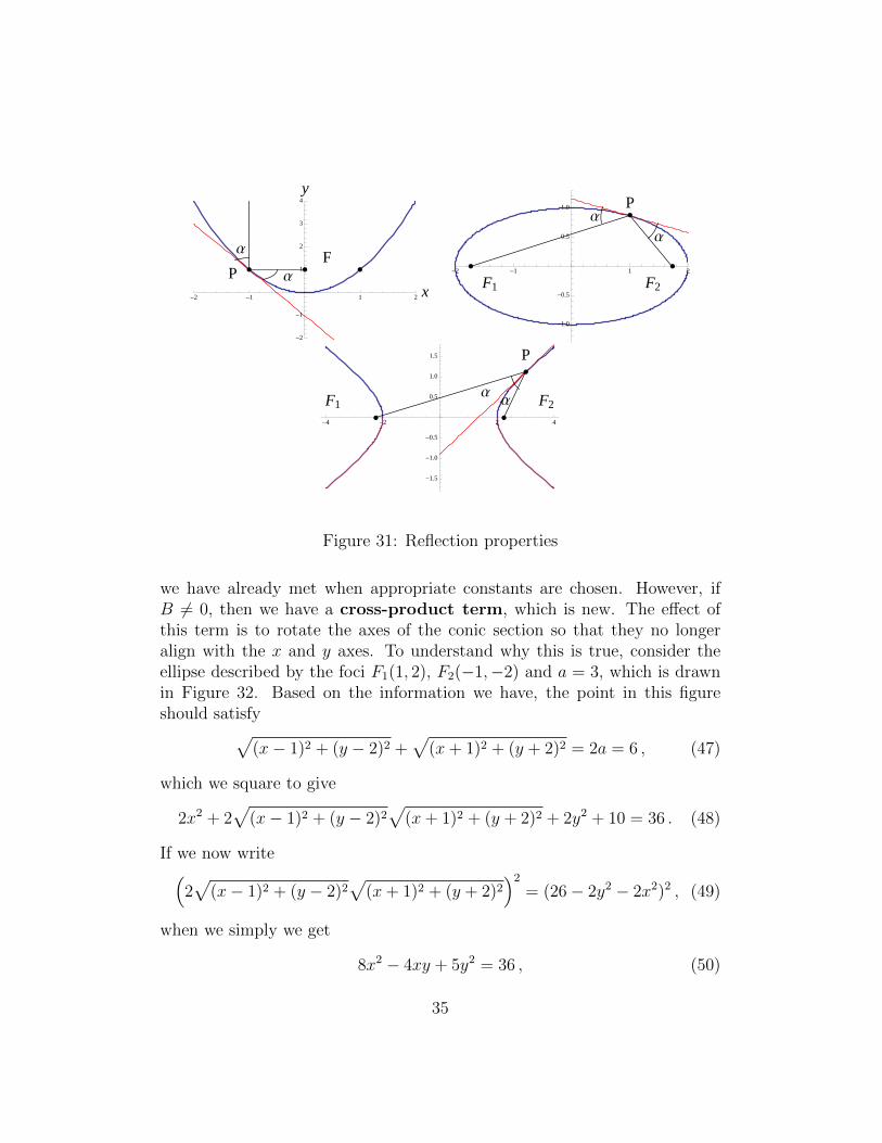
1.3.5 Reflection properties for conic sections

Reflection property of parabolas: Consider a tangent line at a point Pon the parabola. The angles between the tangent line and the line through Pparallel to the focal axis and between the tangent line and the line connectingP to the focus are equal.

Reflection property of ellipses: Consider a tangent line at a point P onthe ellipse. The angles between the tangent line and the lines joining P tothe foci are equal.

Reflection property of hyperbolas: Consider a tangent line at a point Pon the hyperabola. The angles between the tangent line and the lines joiningP to the foci are equal.

These reflection properties are drawn in Figure 31.

1.3.6 Applications of conic sections

Some applications of conic sections include:

Parabola: Parabolic reflector - used in headlights on cars, etc. to project afocussed beam of light.

Ellipse: Planetary orbits - Kepler’s problem. More on this later.

Hyperbola: Scattering of atomic particles - Rutherford’s experiment.

1.4 Rotated conic sections

1.4.1 Quadratic equations

All conic sections are special cases of the general quadratic equation

Ax2 +Bxy + Cy2 +Dx+ Ey + F = 0 . (46)

If A,B,C 6= 0 it is quadratic in x and y, and if they vanish, it reduces to alinear equation in x and y. Obviously B = 0 gives rise to the conic sections

34

FP

Α

Α

-2 -1 1 2 x

-2

-1

1

2

3

4

y

F2F1

P

Α

Α

-2 -1 1 2

-1.0

-0.5

0.5

1.0

F1 F2

P

ΑΑ

-4 -2 2 4

-1.5

-1.0

-0.5

0.5

1.0

1.5

Figure 31: Reflection properties

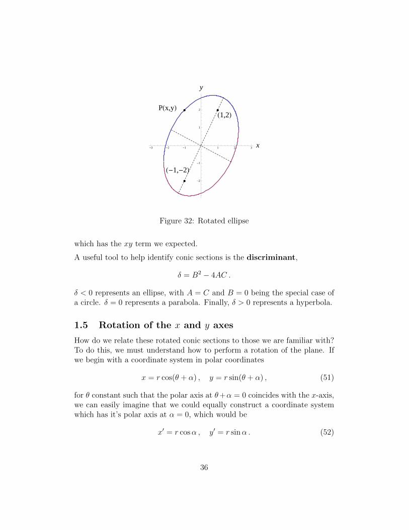
we have already met when appropriate constants are chosen. However, ifB 6= 0, then we have a cross-product term, which is new. The effect ofthis term is to rotate the axes of the conic section so that they no longeralign with the x and y axes. To understand why this is true, consider theellipse described by the foci F1(1, 2), F2(−1,−2) and a = 3, which is drawnin Figure 32. Based on the information we have, the point in this figureshould satisfy√

(x− 1)2 + (y − 2)2 +√

(x+ 1)2 + (y + 2)2 = 2a = 6 , (47)

which we square to give

2x2 + 2√

(x− 1)2 + (y − 2)2√

(x+ 1)2 + (y + 2)2 + 2y2 + 10 = 36 . (48)

If we now write(2√

(x− 1)2 + (y − 2)2√

(x+ 1)2 + (y + 2)2)2

= (26− 2y2 − 2x2)2 , (49)

when we simply we get

8x2 − 4xy + 5y2 = 36 , (50)

35

PHx,yLH1,2L

H-1,-2L

-3 -2 -1 1 2 3 x

-2

-1

1

2

y

Figure 32: Rotated ellipse

which has the xy term we expected.

A useful tool to help identify conic sections is the discriminant,

δ = B2 − 4AC .

δ < 0 represents an ellipse, with A = C and B = 0 being the special case ofa circle. δ = 0 represents a parabola. Finally, δ > 0 represents a hyperbola.

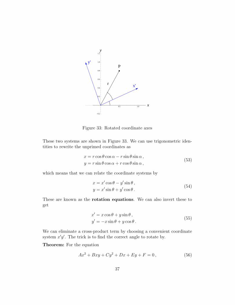
1.5 Rotation of the x and y axes

How do we relate these rotated conic sections to those we are familiar with?To do this, we must understand how to perform a rotation of the plane. Ifwe begin with a coordinate system in polar coordinates

x = r cos(θ + α) , y = r sin(θ + α) , (51)

for θ constant such that the polar axis at θ+α = 0 coincides with the x-axis,we can easily imagine that we could equally construct a coordinate systemwhich has it’s polar axis at α = 0, which would be

x′ = r cosα , y′ = r sinα . (52)

36

P

x'

y'

r

0.5 1.0 x

-0.2

0.2

0.4

0.6

0.8

1.0

1.2

y

Figure 33: Rotated coordinate axes

These two systems are shown in Figure 33. We can use trigonometric iden-tities to rewrite the unprimed coordinates as

x = r cos θ cosα− r sin θ sinα ,

y = r sin θ cosα + r cos θ sinα ,(53)

which means that we can relate the coordinate systems by

x = x′ cos θ − y′ sin θ ,y = x′ sin θ + y′ cos θ .

(54)

These are known as the rotation equations. We can also invert these toget

x′ = x cos θ + y sin θ ,

y′ = −x sin θ + y cos θ .(55)

We can eliminate a cross-product term by choosing a convenient coordinatesystem x′y′. The trick is to find the correct angle to rotate by.

Theorem: For the equation

Ax2 +Bxy + Cy2 +Dx+ Ey + F = 0 , (56)

37

such that B 6= 0, the x′y′-coordinate system obtained by rotating the xy-axesthrough an angle θ satisfying

cot 2θ =A− CB

, (57)

then the equation in x′y′-coordinates becomes

A′x2 + C ′y2 +D′x+ E ′y + F ′ = 0 . (58)

Proof: If we substitute equation (55) into equation (56), we get

A(x′ cos θ − y′ sin θ)2 +B(x′ cos θ − y′ sin θ)(x′ sin θ + y′ cos θ)

+ C(x′ sin θ + y′ cos θ)2 +D(x′ cos θ − y′ sin θ)+ E(x′ sin θ + y′ cos θ) + F = 0 ,

(59)

which means

A′ = A cos2 θ +B cos θ sin θ + C sin2 θ

B′ = B(cos2 θ − sin2 θ) + 2(C − A) sin θ cos θ

C ′ = A sin2 θ −B sin θ cos θ + C cos2 θ

D′ = D cos θ + E sin θ

E ′ = −D sin θ + E cos θ

F ′ = F .

(60)

If we havecos 2θ

sin 2θ= cot 2θ =

A− CB

, (61)

thenB′ = 2B cos 2θ + 2(C − A) sin θ cos θ = 0 (62)

as required.

Example: Rotate to the coordinates that coincide with the axes of the conicsection x2 + 4xy − 2y2 − 6 = 0. What type of conic section is it?

Solution: We need to rotate by θ, where

cot 2θ =1− (−2)

4=

3

4⇒ θ = 0.463648 rad = 26.5651o

⇒ sin θ = 0.447214 , cos θ = 0.894427 .

38

Using these, we can substitute into equation (60) to get

A′ = 2 , B′ = 0 , C ′ = −3 , F ′ = −6 ,

where of course, D′ = E ′ = 0 since there are no linear terms initially. Theequation in the new variables is therefore

2x′2 − 3y′2 = 6

⇒x′2

3− y′2

2= 1 ,

which is a hyperbola.

1.6 Conic Sections in Polar Coordinates

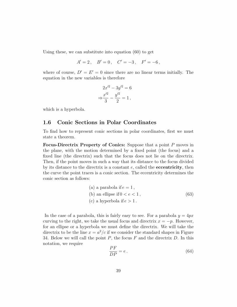
To find how to represent conic sections in polar coordinates, first we muststate a theorem.

Focus-Directrix Property of Conics: Suppose that a point P moves inthe plane, with the motion determined by a fixed point (the focus) and afixed line (the directrix) such that the focus does not lie on the directrix.Then, if the point moves in such a way that its distance to the focus dividedby its distance to the directrix is a constant e, called the eccentricity, thenthe curve the point traces is a conic section. The eccentricity determines theconic section as follows:

(a) a parabola if e = 1 ,

(b) an ellipse if 0 < e < 1 ,

(c) a hyperbola if e > 1 .

(63)

In the case of a parabola, this is fairly easy to see. For a parabola y = 4pxcurving to the right, we take the usual focus and directrix x = −p. However,for an ellipse or a hyperbola we must define the directrix. We will take thedirectrix to be the line x = a2/c if we consider the standard shapes in Figure34. Below we will call the point P , the focus F and the directrix D. In thisnotation, we require

PF

DP= e . (64)

39

FHc,0L

FHx,yLD

x=-p

e=1

-1 1 2 3 x

-2

-1

1

2

y

FHc,0L

PHx,yL

x=a2�c0<e<1

D

-2 -1 1 2 x

-1.5

-1.0

-0.5

0.5

1.0

y

FHc,0L

PHx,yL

x=a2�ce>1

D

-4 -2 2 4 x

-1.5

-1.0

-0.5

0.5

1.0

1.5

y

Figure 34: Conic sections defined and eccentricities

For a parabola, we already know that the distance PF to the focus is equalto the distance to the directrix PD, so e = 1. For the ellipse, Recalling thefifth line of equation 34, we have√

(x− c)2 + y2 =c

a

(a2

c− x), (65)

where the left-hand side is PF , and the bracketed term on the right is PD.Therefore, for an ellipse,

e =c

a, (66)

which given 0 < c < a gives 0 < e < 1, unless a = 0 or c = 0. What wouldthe conic section be in these situations? Finally, for the hyperbola, we knowthat the distance to the further focus minus the distance to the nearer focusis 2a. Therefore, in analogy with equation (34), we get√

(x+ c)2 + y2 −√

(x− c)2 + y2 = 2a , (67)

so performing the same procedures, we arrive at√(x− c)2 + y2 =

c

a

(x− a2

c

), (68)

40

where the left-hand side is again PF and the right-hand side is PD sincethe directrix is the opposite side to the point compared with the case of theellipse. Therefore, we also have

e =c

a, (69)

for a hyperbola.

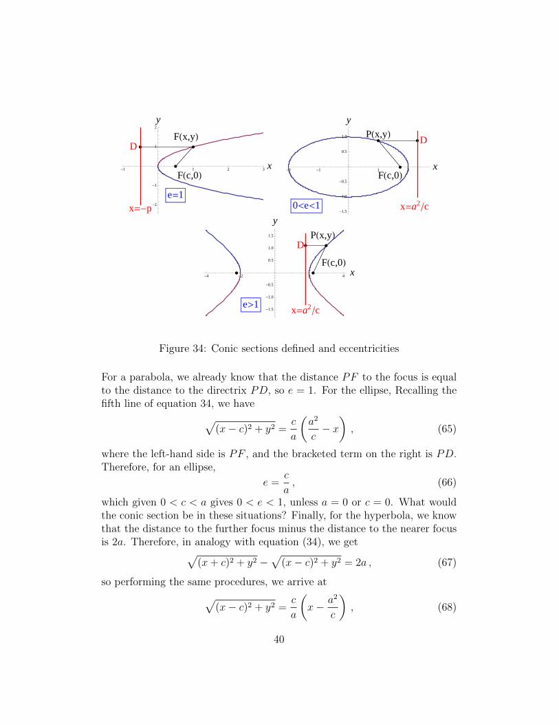
Also note that for an ellipse, eccentricity can be regarded as a measure of theflatness of the ellipse: as e approaches 0, the ellipse becomes circular; as eapproaches 1 the ellipse flattens out. Earth’s orbit has e = 0.017. See Figure35 for plot of ellipses of different eccentricites.

F

e=0e=0.2e=0.4e=0.6e=0.8

-1.0 -0.5 0.5 1.0 1.5 2.0

-1.0

-0.5

0.5

1.0

Figure 35: Ellipses with same focus and same semi-major axis, but differenteccentricities

1.6.1 Polar equations of conics

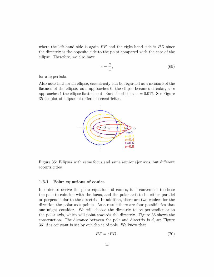
In order to derive the polar equations of conics, it is convenient to chosethe pole to coincide with the focus, and the polar axis to be either parallelor perpendicular to the directrix. In addition, there are two choices for thedirection the polar axis points. As a result there are four possibilities thatone might consider. We will choose the directrix to be perpendicular tothe polar axis, which will point towards the directrix. Figure 36 shows theconstruction. The distance between the pole and directrix is d, see Figure36. d is constant is set by our choice of pole. We know that

PF = ePD . (70)

41

F

Pole

Θ

r

r cos Θ

PHx,yL

d

D

Figure 36: Polar coordinates defined for conics

For the situation in the diagram, we have PF = r and PD = d− r cos θ, andtherefore

r =ed

1 + e cos θ. (71)

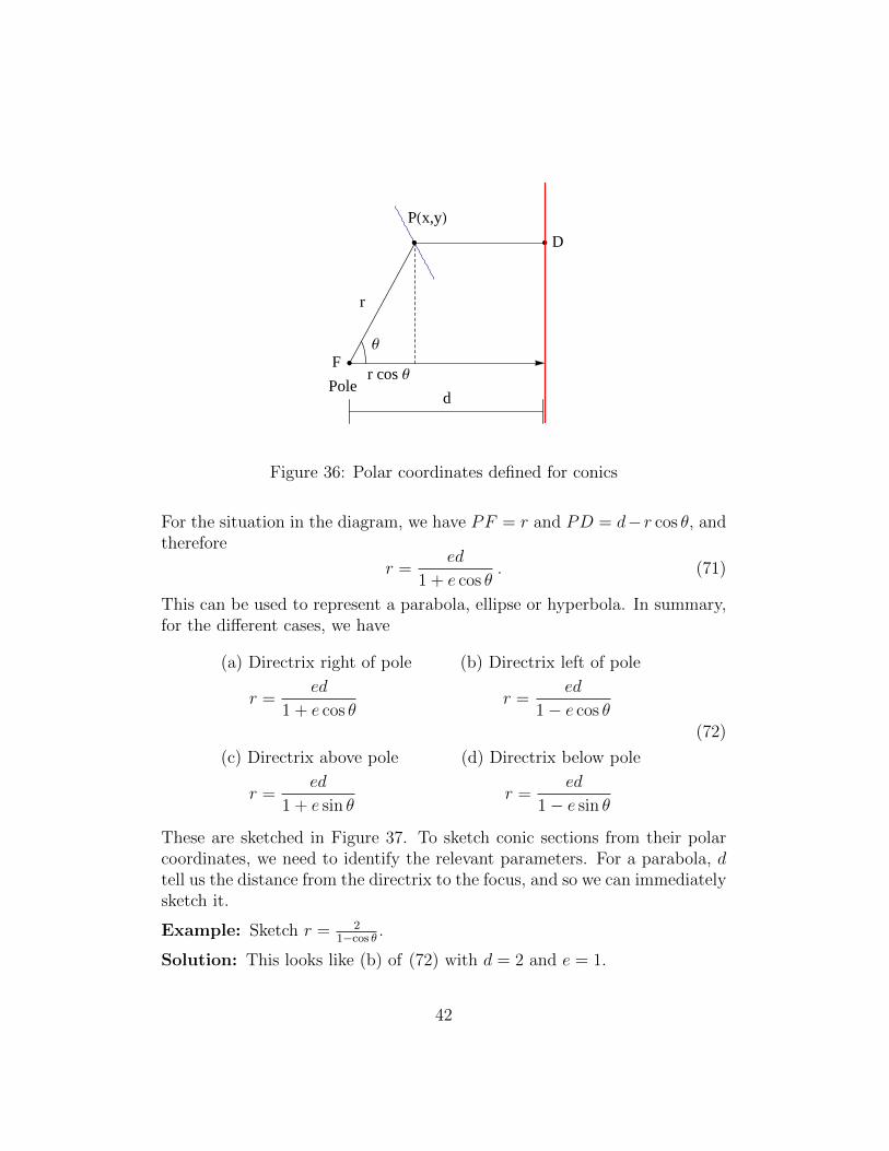
This can be used to represent a parabola, ellipse or hyperbola. In summary,for the different cases, we have

(a) Directrix right of pole (b) Directrix left of pole

r =ed

1 + e cos θr =

ed

1− e cos θ

(c) Directrix above pole (d) Directrix below pole

r =ed

1 + e sin θr =

ed

1− e sin θ

(72)

These are sketched in Figure 37. To sketch conic sections from their polarcoordinates, we need to identify the relevant parameters. For a parabola, dtell us the distance from the directrix to the focus, and so we can immediatelysketch it.

Example: Sketch r = 21−cos θ

.

Solution: This looks like (b) of (72) with d = 2 and e = 1.

42

F

D

HaL

F

D

HbL

F

DHcL

F

D

HdL

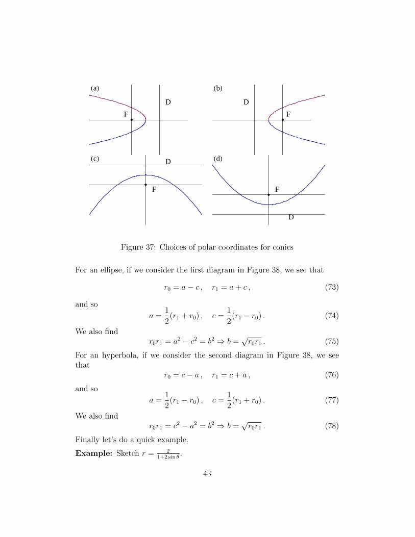
Figure 37: Choices of polar coordinates for conics

For an ellipse, if we consider the first diagram in Figure 38, we see that

r0 = a− c , r1 = a+ c , (73)

and so

a =1

2(r1 + r0) , c =

1

2(r1 − r0) . (74)

We also findr0r1 = a2 − c2 = b2 ⇒ b =

√r0r1 . (75)

For an hyperbola, if we consider the second diagram in Figure 38, we seethat

r0 = c− a , r1 = c+ a , (76)

and so

a =1

2(r1 − r0) , c =

1

2(r1 + r0) . (77)

We also findr0r1 = c2 − a2 = b2 ⇒ b =

√r0r1 . (78)

Finally let’s do a quick example.

Example: Sketch r = 21+2 sin θ

.

43

a a

ab

r0r1

c-3 -2 -1 1 2 3

-2

-1

1

2

c

a

b

r0r1

-5 5

-5

5

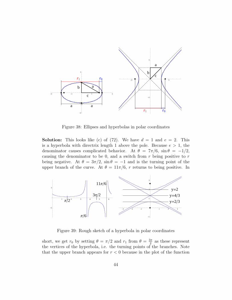
Figure 38: Ellipses and hyperbolas in polar coordinates

Solution: This looks like (c) of (72). We have d = 1 and e = 2. Thisis a hyperbola with directrix length 1 above the pole. Because e > 1, thedenominator causes complicated behavior. At θ = 7π/6, sin θ = −1/2,causing the denominator to be 0, and a switch from r being positive to rbeing negative. At θ = 3π/2, sin θ = −1 and is the turning point of theupper branch of the curve. At θ = 11π/6, r returns to being positive. In

Π�6

11Π�6

Π�2

3Π�21 2 3 4 5 6

-5

5

y=2�3

y=4�3

y=2

-3 -2 -1 1 2 3

-1

1

2

3

Figure 39: Rough sketch of a hyperbola in polar coordinates

short, we get r0 by setting θ = π/2 and r1 from θ = 3π2

as these representthe vertices of the hyperbola, i.e. the turning points of the branches. Notethat the upper branch appears for r < 0 because in the plot of the function

44

it is below the axis. The function and the hyperbola are drawn in Figure 39.Then,

r0 =2

1 + 2 sin π/2=

2

3, r1 =

∣∣∣∣∣ 2

1 + 2 sin 3π/2

∣∣∣∣∣ =2

| − 1|= 2 . (79)

Therefore

a =1

2(r1 − r0) =

2

3, b =

√r0r1 =

2√

3

3, c =

1

2(r1 + r0) =

4

3. (80)

1.6.2 Planetary motion

While you might see more of this in a mechanics course, we will here state

Kepler’s Laws of Planetary Motion:

1. Law of Orbits: The motion of each planet traces an ellipse with theSun at one of the foci.

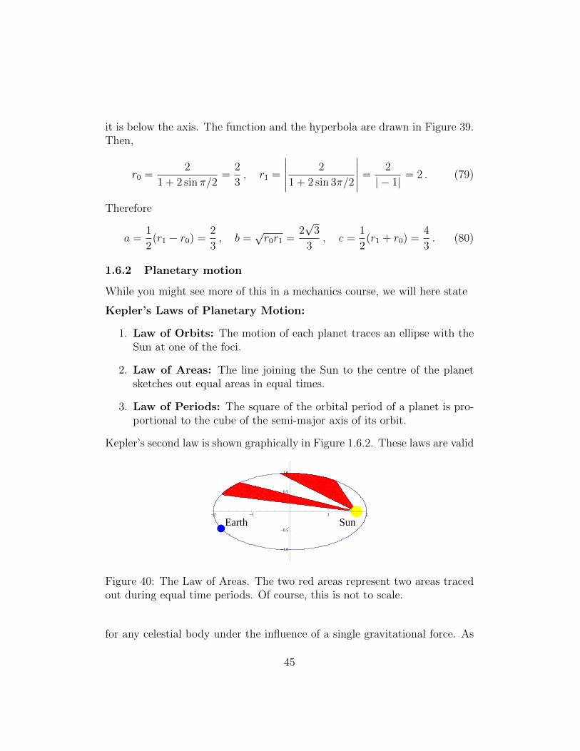
2. Law of Areas: The line joining the Sun to the centre of the planetsketches out equal areas in equal times.

3. Law of Periods: The square of the orbital period of a planet is pro-portional to the cube of the semi-major axis of its orbit.

Kepler’s second law is shown graphically in Figure 1.6.2. These laws are valid

SunEarth-2 -1 1 2

-1.0

-0.5

0.5

1.0

Figure 40: The Law of Areas. The two red areas represent two areas tracedout during equal time periods. Of course, this is not to scale.

for any celestial body under the influence of a single gravitational force. As

45

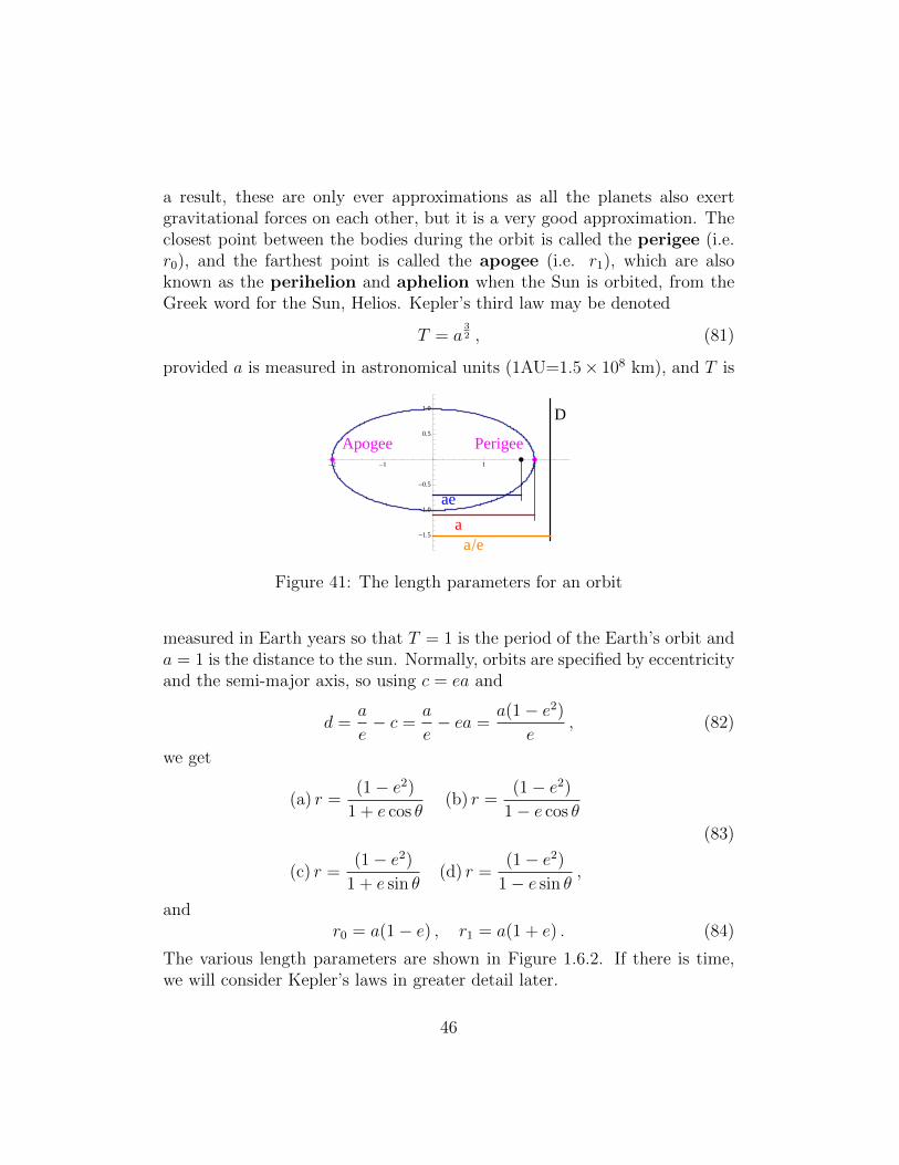
a result, these are only ever approximations as all the planets also exertgravitational forces on each other, but it is a very good approximation. Theclosest point between the bodies during the orbit is called the perigee (i.e.r0), and the farthest point is called the apogee (i.e. r1), which are alsoknown as the perihelion and aphelion when the Sun is orbited, from theGreek word for the Sun, Helios. Kepler’s third law may be denoted

T = a32 , (81)

provided a is measured in astronomical units (1AU=1.5× 108 km), and T is

D

ae

a

a�e

Apogee Perigee-2 -1 1 2

-1.5

-1.0

-0.5

0.5

1.0

Figure 41: The length parameters for an orbit

measured in Earth years so that T = 1 is the period of the Earth’s orbit anda = 1 is the distance to the sun. Normally, orbits are specified by eccentricityand the semi-major axis, so using c = ea and

d =a

e− c =

a

e− ea =

a(1− e2)

e, (82)

we get

(a) r =(1− e2)

1 + e cos θ(b) r =

(1− e2)

1− e cos θ

(c) r =(1− e2)

1 + e sin θ(d) r =

(1− e2)

1− e sin θ,

(83)

andr0 = a(1− e) , r1 = a(1 + e) . (84)

The various length parameters are shown in Figure 1.6.2. If there is time,we will consider Kepler’s laws in greater detail later.

46