1

Multivariable and Closed-Loop Identification

for Model Predictive Control

Yucai Zhu*

Faculty of Electrical Engineering, Eindhoven University of TechnologyP.O. Box 513, 5600 MB Eindhoven, The Netherlands

Phone +31.40.2473246, y.zhu@tue.nl

Firmin ButoyiDow Benelux N.V.

P.O. Box 48, 4530 AA Terneuzen, The Netherlands

*Also with: Tai-Ji ControlHageheldlaan 62, NL-5641 GP Eindhoven, The NetherlandsPhone +31.40.2817192, fax +31.40.2813197, y.zhu@tip.nl

Abstract: In this work we will study multivariable and closed-loop identification of largescale industrial processes for use in model predictive control (MPC). The advantages ofclosed-loop identification will be discussed and related problems of identification areoutlined. Then, asymptotic method (ASYM) of identification is introduced. The fourproblems, test signal design for control, model order/structure selection, parameter estimationand model validation, are solved in a systematic manner. The method provides accurateinput/output model and unmeasured disturbance model, model errors are quantified by anupper error bound matrix that can be used for model validation and test redesign. Todemonstrate the use of the method, the identification of a deethanizer for use in MPC will bepresented.

1 IntroductionModel predictive control (MPC) technology has been widely applied in refinery andpetrochemical industries and is beginning to attract interest from other process industries.Dynamic models play a central role in MPC technology. Generally identified black-boxmodels are used for MPC controllers. Industrial project experience has shown that the mostdifficult and time-consuming work in an MPC project is modelling and identification. Typicalidentification test will take several weeks. These long tests make production planningdifficult. The tests are done manually, which dictates extremely high commitment of theengineers and operators and the quality of collected data depends heavily on the technicalcompetence and experience of the control engineer and the operator. The data collected fromthese long tests may not be good enough for model identification due to not enough excitationand process nonlinearity. After the test, due to the lack of systematic identification approach,it can take another few weeks to analyse the data and to identify the models. Some peopleeven believe that the long time needed for tests and data analysis is the price one must pay fora good model.

The high cost of identification of current industrial approach is caused by several factors. Firstsingle variable tests make the test time unnecessarily long. Secondly, open-loop tests are used

2

in industrial MPC projects. When the process is sensitive and/or non-linear, such as a highpurity distillation column, it is very difficult to carry out open-loop tests on the process.Upsets often occur and it is difficult to fit a linear model when controlled variable variationsare too large. Finally, most industrial identification packages are based on FIR model that is anonparametric model with a large number of parameters.

In control community, system (process) identification has been one of the most activebranches in the last three decades. An astonishing fact is that most of the identification resultsdeveloped in the last 30 years are not used by industrial control engineers, although there is anurgent need for efficient and effective identification methods in process control industry.

In the last decade, there is a renewed interest in closed-loop identification and control-relevantidentification; see van den Hof (1997) for a recent summary of the work. Many identificationschemes have been proposed. Unfortunately, most researchers involved in closed-loopidentification assume that the existing controller is linear and the process is single variable.This makes their result not relevant for use in the framework of MPC, because a MPCcontroller is nonlinear and the process under control is multivariable. Although called“conventional” by many researchers, the prediction error method of Ljung (1987) is still amore powerful methodology than many newly proposed schemes for use in closed-loopidentification for MPC.

Recently, Zhu (1998) has developed a so-called ASYM method that uses automatedmultivariable tests and parametric models. Better models can be obtained with much shortertest and over 60% time saving is reported.

In this work we will continue the development of Zhu (1998) and study closed-loopidentification. In Section 2 the characteristics of refinery/petrochemical processes arediscussed and closed-loop identification is motivated. In Section 3 the ASYM method isintroduced where closed-loop test design and model validation will be emphasised. In Section4, the ASYM is used to identify a deethanizer for MPC control. Section 5 contains theconclusions and perspectives.

2 Closed-Loop Identification, Why and How?Closed-loop identification means that process model is identified using data collected from aclosed-loop test where the underlying process is fully or partly under feedback control. In thissection we will motivate the use of closed-loop identification from both process operationpoint of view and control theoretical point of view and discuss various issues around closed-loop identification. We will focus our discussion on hydrocarbon process industry (HPI)processes where MPC application is most challenging and also most beneficial. This class ofprocesses can be characterised as follows:

1) Large scale and complex. A large size MPC will have 10 to 20 MVs and 20 to 40 CVs.Some CVs, such as product qualities, are very slow (with dominant time constant rangefrom 30 minutes to several hours), and other CVs are very fast, such as valve positions(with time constant in few minutes). There exist inverse responses, oscillations and timedelays.

2) Dominant slow dynamics. The time to steady state of a typical product quality modelranges from one hour to several hours. This dictates long identification test.

3) High level and slow disturbances. Typical sources of unmeasured disturbances are feedcomposition variations, weather changes and disturbances from other part of the unit.

3

These are slow and irregular variations. During an identification test, the level ofdisturbances is in average above 10% of that of CV variation (in power), but it can bemuch higher. Too large test signal amplitudes are not permitted because they will causeoff-specification of product and/or will excite nonlinearity.

4) Local nonlinearity. Although in general linear models are relevant for MPC for this classof processes for a given range of operation, some nonlinear behaviour may still show up.Examples are CVs that are very pure product qualities and valve positions close to theirlimits.

Based on these observations we will outline the special needs in HPI process identification forMPC and give comments on the existing methods. The discussion will be around the fourproblems of identification: test design, model structure and parameter estimation, orderselection and model validation.

1) Identification Test

A good identification test plays a key role in a successful identification. Current practice ofMPC industry is to use a series of open loop and single-variable step tests. The tests arecarried out manually. The advantage of this test method is that control engineer can watchmany step responses during the tests and can learn about the process behaviour in an intuitivemanner. The biggest problem of single variable step test is its high cost in time and inmanpower. The second problem is that the data from single variable test may not contain goodinformation about the multivariable character of the process (ratios between different models)and that step signals do not excite enough dynamic information of the process.

Using automatic multivariable test can solve these problems; see Zhu (1998). In an open-loopmultivariable test, many, or, all MVs are perturbed using some test signals such as PRBSsignals. If the process behaves linearly in the operating range, levels of disturbance are lowand the operation constraints are not very tight, one can use open-loop test without problems.

However, as mentioned before, HPI processes often suffer from high level disturbances andwill be nonlinear in a wide range. In such cases, identification tests can be done in closed-loopoperation with part or all the CVs under feedback control. There are many advantages ofclosed-loop test:

• Reduce the disturbance to process operation and eliminate product off-specification.When a multivariable open-loop test is used, some of the CVs may drift away and operatorneeds to intervene in order to prevent product qualities from off-specification. In a closed-loop test, however, one can specify the amplitude of the setpoint movement and thecontroller will help to keep the CVs within their operation limits.

• Easy to carry out. During an identification test, to obtain sufficiently high signal-to-noiseratio and to maintain all the CVs in their operation constraints are often in conflict. It ismost difficult to perform manual single-variable step tests. It demands very highcommitment of the control engineer and of the operator if the process is sensitive and hastight constraints. An automatic multivariable open-loop test will be much easier, butoperator intervention may still be necessary to keep the CVs within their limits. The workwill become easiest if the process is under feedback control.

• Better model for control. This can be explained in several aspects. Under the same CVvariance constraints, the control performance degradation caused by model errors will beless if closed-loop test is carried out; see Gevers and Ljung (1986) and Hjalmarsson et. al.(1996). In fact, CV variances in a closed-loop test can be actually larger than those in an

4

open loop test, because the process operation constraints are in CV amplitude limits, not invariance limits and the controller can remove the slow drifts of the CVs. This means thatthe signal-to-noise ratio can be higher in a data set from a closed-loop test. The effect offeedback will have additional advantage if the process is ill conditioned meaning thatseveral CVs are strongly correlated. High purity distillation columns are often illconditioned where top and bottom compositions have strong correlation. For the control ofill-conditioned processes, it is important to identify the model that has good estimate oflow-gain direction. In an open loop test where MVs are moved independently, theinformation of low gain direction will have very low power and cannot be estimatedaccurately from noisy data. In order to amplify the power of low-gain direction, certaincorrelation between MV movement is needed. This correlation can be created naturally by(partial) feedback control; see Koung and MacGregor (1993) and Jacobsen (1994).

Remark on the feedback controller

The controller is used to keep important CVs within their operation constraints during theidentification test. It can be one or several PID loops or it is an existing MPC controller. Forexample, when testing a distillation column, it is often sufficient to control the top and bottomcompositions or (pressure compensated) temperatures using two PID controllers. If only onequality is sensitive and has tight constraints, one PID controller will be sufficient. Thesecontrollers often exist for HPI processes due to the evolution of advanced process control inHP industry.

Remark on process identifiability in closed-loop test

Some researchers and engineers have mistakenly believed that the process is only identifiablewhen open-loop test is performed and when MVs are moved independently. This may explainwhy so little closed-loop identification applications have been reported. It has been shownlong time ago that, if persistent excitation signals are added on the MVs and/or on the CVsetpoints, the process will be identifiable in a closed-loop test, provided a right modelstructure is used; see Gustavsson et. al. (1977). It is true that some model structures and someestimation methods will be biased and not consistent if used for closed-loop identification; seethe next paragraph.

Test signal design is another important issue that will be discussed in the next section.

2) Model Structure and Parameter Estimation

Before further discussion, let us introduce some notations. Given a multivariable process withm manipulated variables (MVs or inputs) and p controlled variables (CVs or outputs). Denotethe data sequence collected from an identification test as

)}(),(),......,2(),2(),1(),1({: NyNuyuyuZ N = (2.1)

where u(t) is m-dimensional input vector (MVs), y(t) is p-dimensional output vector (CVs)and N is the number of samples.

We assume that a linear discrete-time process generates the data

y t G z u t H z e to o( ) ( ) ( ) ( ) ( )= +− −1 1 (2.2)

where z-1 is the unit time delay operator, Go(z-1) is the process transfer function matrix, Ho(z-1)is the noise filter and e(t) is a p-dimensional white noise vector. Here the term Ho(z-1)e(t)represent the unmeasured disturbances acting at the process outputs.

The model to be identified is in the same structure as in (2.1):

5

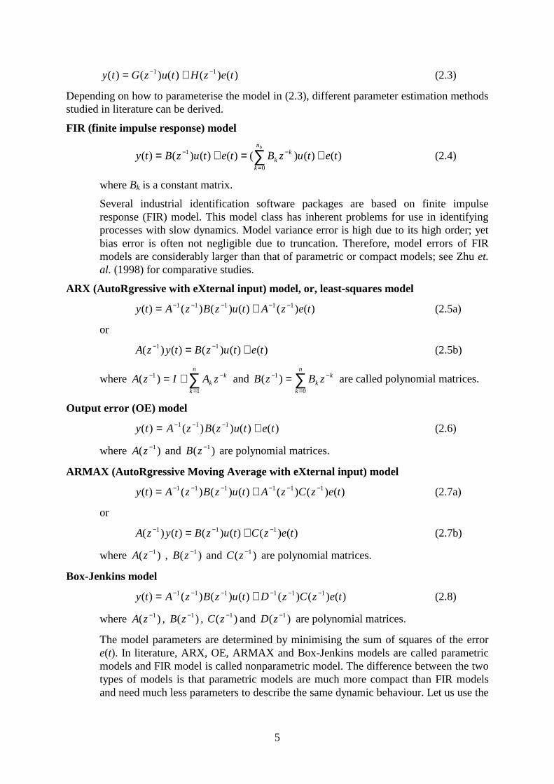
y t G z u t H z e t( ) ( ) ( ) ( ) ( )= +− −1 1 (2.3)

Depending on how to parameterise the model in (2.3), different parameter estimation methodsstudied in literature can be derived.

FIR (finite impulse response) model

)()()()()()()(0

1 tetuzBtetuzBtybn

k

kk +=+= ∑

=

−− (2.4)

where Bk is a constant matrix.

Several industrial identification software packages are based on finite impulseresponse (FIR) model. This model class has inherent problems for use in identifyingprocesses with slow dynamics. Model variance error is high due to its high order; yetbias error is often not negligible due to truncation. Therefore, model errors of FIRmodels are considerably larger than that of parametric or compact models; see Zhu et.al. (1998) for comparative studies.

ARX (AutoRgressive with eXternal input) model, or, least-squares model

)()()()()()( 11111 tezAtuzBzAty −−−−− += (2.5a)

or

)()()()()( 11 tetuzBtyzA += −− (2.5b)

where ∑=

−− +=n

k

kk zAIzA

1

1)( and ∑=

−− =n

k

kk zBzB

0

1)( are called polynomial matrices.

Output error (OE) model

y t A z B z u t e t( ) ( ) ( ) ( ) ( )= +− − −1 1 1 (2.6)

where )( 1−zA and )( 1−zB are polynomial matrices.

ARMAX (AutoRgressive Moving Average with eXternal input) model

)()()()()()()( 111111 tezCzAtuzBzAty −−−−−− += (2.7a)

or

)()()()()()( 111 tezCtuzBtyzA −−− += (2.7b)

where )( 1−zA , )( 1−zB and )( 1−zC are polynomial matrices.

Box-Jenkins model

)()()()()()()( 111111 tezCzDtuzBzAty −−−−−− += (2.8)

where )( 1−zA , )( 1−zB , )( 1−zC and )( 1−zD are polynomial matrices.

The model parameters are determined by minimising the sum of squares of the errore(t). In literature, ARX, OE, ARMAX and Box-Jenkins models are called parametricmodels and FIR model is called nonparametric model. The difference between the twotypes of models is that parametric models are much more compact than FIR modelsand need much less parameters to describe the same dynamic behaviour. Let us use the

6

degree of polynomial matrix as a measure of model compactness. Then a model is saidto be more compact if the polynomial degree is lower.

Subspace method

In recent years, the so called subspace method of parameter estimation has beenproposed and studied in the literature; see van Overschee and de Moor (1994),Verhaegen (1994) and Larimore (1990). Subspace methods estimate state space modelof a multivariable process directly from input/output data. A state space model of alinear process with disturbance can be given as

)()()()(

)()()()1(

tetDutCxty

tKetButAxtx

++=++=+

(2.9)

where x(t) is the state vector of dimension nA, the constant matrices A, B, C and Dform the state space description of the process and constant matrix K is the Kalmangain that characterise the state noise, e(t) is a p dimensional white noise vector.

For closed-loop identification, the choice of model structure depends on three and oftenconflict issues:

1) the compactness of the model2) the numerical complexity in parameter estimation3) the consistency of the model in closed-loop identification.

When noisy data is used in identification, a more compact model will be more accurateprovided that the parameter estimation algorithm converges to global minimum and the modelorder is selected properly; see Section 3.

Among the parametric models, one would like to have the model that is most accurate or, inidentification term, minimum variance. In general a model structure or an estimation methodthat includes a disturbance model will be better than a method without the disturbance model;see Ljung (1987) and Söderström and Stoica (1989). Prediction error criterion and maximumlikelihood criterion belongs to the first class; while output error criterion belongs to thesecond class. At present it is not clear what criterion subspace methods use. Moreover,prediction error method and maximum likelihood method will give consistent estimate forclosed-loop data meaning that the effect of the disturbance will decrease when test timeincreases; while output error criterion will deliver biased model when using closed-loop data.The consistency of subspace methods can only be proven in for open-loop test case; seeJansson and Wahlberg (1996).

However, a more compact model needs more complex parameter estimation algorithms. Toestimate OE models, Box-Jenkins models and ARMAX models, nonlinear optimisationroutines are needed which often suffer from local minima and convergence problems whenidentifying a multivariable process. In FIR and ARX models, the error term e(t) is linear in theparameters; see (2.4) and (2.5b). Due to this property, linear least-squares method can be usedin parameter estimation that is numerically simple and reliable, and no problem of localminimum and convergence will occur. This explains partly why FIR model is often used inindustrial identification. The subspace methods are exceptional: they estimate a parametricmodel and they are numerically efficient. The main part of a subspace method consists ofmatrix singular value decomposition (SVD) and linear least-squares estimation which arenumerically simple and reliable.

7

Recently, orthonormal basis functions are studied for use in identification; see, e.g., Wahlberg(1991) and van den Hof et. al. (1995). One of the motivations of using this class of models isto estimate an output error model using the numerically simple least-squares method.

To summarise the discussion, the following table compares the advantages and disadvantagesof various model structures or parameter estimation methods. It is clear that Box-Jenkinsmodel is the best candidate for closed-loop identification, provided that parameter estimationand order selection problems can be solved.

Table 2.1 Comparison of various model structures and estimation methods

Model structure orestimation method

Numericaldifficulty

Compactness Consistency inclosed-loop test

FIR Low Low No ARX (high order) Low Medium Yes

OE High Highest No ARMAX High High Yes

Box-Jenkins High Highest Yes Subspace method Low High No

Orthonormal basis function Medium Medium No

3) Order Selection

In identification literature, when prediction error is used in parameter estimation, it is alsoused in order selection. We will argue that, although prediction error is a good choice forparameter estimation, it is not the best criterion for order selection for control. For the purposeof control, it is most important to select the model order so that the process model )( 1−zG ismost accurate. In the time domain, this requires that the simulation error or, output error of themodel be minimal; see Zhu (1988b) for more details and an example. In the frequencydomain, this requires that the bias part and the variance part of the model are nearly equal sothat the total error is minimal; see Section 3.

4) Model Validation

The goal of model validation is to test whether the model is good enough for its purpose andto provide advise for possible re-identification if the identified model is not valid for itsintended use. Commonly used methods of model validation are simulation using estimationdata or fresh data, whiteness test of model residuals and testing the independence between theresiduals and past MVs. These methods only tell how well the model agrees with the test data.They can neither quantify the model quality with respect to the purpose of modelling, in ourcase, closed-loop control, nor can they give good advice for re-identification. In this way, thefundamental problem of model validation is basically unsolved in both literature and practice,especially for multivariable processes. Trial-and-error approach in this step makes industrialidentification a very expensive practice. In linear model identification for control, a logicalapproach for model validation is to quantify model errors in the frequency domain and to findrelationship between this kind of error description and model based control performance.Model error estimation has attracted much interest in the last decade, which is motivated bylinear robust control theory.

The above mentioned four problems are fundamental in industrial process identification.Solving these problems in a systematic manner is a challenging task. In the next section the so

8

called ASYM method of identification is introduced that provide industrial solutions to theseproblems.

3 Asymptotic Method of Identification The asymptotic method (ASYM) of identification was developed for the purpose model basedcontrol; see Zhu (1998).

Denote frequency responses of the process (2.2) and of the model (2.3) are denoted as

)](),([:)( ωωω ioioio eHeGcoleT =

� ( ): [ � ( ), � ( )]T e col G e H en i n i n iω ω ω=

where n is the degree of the polynomials of the model, col(.) denotes the column operator.

The Asymptotic Properties of Prediction Error Method Assume that

n and n N as N→ ∞ → → ∞2 0/

Test signals have continuous none zero spectra until the Nyquist frequency.

Then (Ljung, 1986 and Zhu 1989)

� ( ) ( )T e T e as Nn i o iω ω→ → ∞ (3.1)

The errors of � ( )T en iω follows a Gaussian distribution, with covariance given as

)()()(ˆcov[ ωω vTiwn

N

neT Φ⊗Φ≈ − (3.2)

where Φ( )ω is the spectrum matrix of inputs and prediction error residual col u t tT T[ ( ), ( )]ξ ,

Φv ( )ω is spectrum matrix of unmeasured disturbances, ⊗ denotes the Kronecker product and-T denotes inverse and then transpose.

Note that the theory holds for the general case of closed-loop test. For open-loop test, thefollowing simplified results can be obtained for process model

cov[ [ � ( )] ( ) ( )col G en

Nn iw

uT

v≈ ⊗−Φ Φω ω (3.3)

where Φu ( )ω is the spectrum matrix of inputs.

In the following, we will outline the ASYM method that makes extensive use of theasymptotic theory. In order to minimise the presentation complexity, we will outline themethod for open-loop experiment and also assume that the test inputs are mutuallyindependent.

The Procedure of the Asymptotic Method

1) Identification Test

9

One should realise that a theory for practical identification test design does not exist and,therefore, project experience and control engineering intuition are combined with theasymptotic theory in developing the ASYM test scheme. The following are the importantfeatures of the ASYM test:

a) Duration of identification test. The duration of ASYM is determined by severalfactors: the validation of the asymptotic expression, the process time to steady state(settling time), and the number of MVs. The experience has shown that whencompared to traditional step test, 70% of test time can be saved using multivariabletest. Note that this test is designed for parametric model identification. The test timemay not be long enough for nonparametric FIR models, because the identification ofnonparametric models needs much longer test time; see Zhu et. al. (1999).

b) (Partial) Closed-loop test. When the level of disturbance is not high and all the CVshave large operation ranges, it will be easy to test the process in open loop operation.But often some CVs are sensitive and have tight constraints; open loop test may bedifficult to carry out. In this situation, closed-loop will be used with these sensitiveCVs being controlled by some single loop PID controllers or by an existing MPCcontroller.

When single loop controllers are used, the test signals are applied to the MVs whichare not under feedback control and the setpoints of the CVs which are under control. Ifan MV under closed-loop test does not move sufficiently due to too slow controlaction, additional test signal can be added on that MV.

c) Spectra of test signals. The optimal test signal is designed to minimise the sum of thesquares of the simulation error (often called prediction error in MPC term). In open-loop test, the spectra of the test signals are based on the following formula which canbe derived from (3.6) assuming open-loop test (Ljung and Yuan, 1985):

Φ Φ Φuj

optj u j

simvi

i

p

( ) ( ) ( )ω µ ω ω==∑

1

(3.4)

where )(ωsimu j

Φ is the spectrum of the j-th input movement in a controlled system, µj is

a constant which is adjusted to meet the amplitude constraint of the signal. In closed-loop test, the following formula can derived for the single variable case (Zhuand van den Bosch, 1999)

)()()( ωωµω vroptr ΦΦ≈Φ (3.5)

where )(ωrΦ is the reference signal at setpoint of the closed-loop system.

In practice, (3.4) or (3.5) is used in combination with upper error bound (3.9) to givegeneral guidelines for the test design. The spectra of the test signals can be realised byPRBS (pseudo-random-binary-sequence) signals or filtered white noises.

10

Before model identification, some data pre-treatment is carried out. This includes removingthe spikes, data slicing, hi-pass filtering (de-trending), known delay correction and signalscaling. This part of the work is well known; see Ljung (1987) and Zhu and Backx (1993).

2) Estimate a high order ARX (equation error) model

� ( ) ( ) � ( ) ( ) �( )A z y t B z u t e tn n− −= +1 1 (3.6)

where � ( )A zn −1 is a diagonal polynomial matrix and � ( )B zn −1 is full polynomial matrix, both

with degree n polynomials. Denote � ( )G zn −1 as the high order ARX model of the process, and� ( )H zn −1 as the high order model of the disturbance.

3) Perform frequency weighted model reduction (ML estimate)

The high order model in (3.6) is practically unbiased, provided that the process behaves lineararound the working point. The variance of this model is high due to its high order. Here weintend to reduce the variance by perform a model reduction on the high order model. If weview the frequency response of the high order estimates as the noisy observations of the truetransfer function, we can then apply the maximum likelihood principle. Using the asymptoticresult of (3.1) and (3.3), we can show that the asymptotic negative log-likelihood function forthe reduced process model is given by (Wahlberg, 1989, Zhu and Backx, 1993)

V = |{| � ( ) � ( )| [ ( )] ( )}|dG Gijn

ij jj v ij

m

i

p

ω ω ω ω ωω

ω

− − − −

==∫∑∑ 2 1 1 1

1

2

11

Φ Φ (3.7)

The reduced model � ( )G z−1 is thus calculated by minimizing (3.7) for a fixed order. The same

can be done for the disturbance model � ( )H zn −1 = 1 1/ � ( )A zn − .

There are some theoretical evidence that the high order plus model reduction approach willproduce more accurate models than that obtained using direct estimation of low order models;see Tjärnström and Ljung (1999).

4) Use asymptotic criterion (ASYC) for order selection

The best order of the reduced model is determined using a frequency domain criterion ASYCwhich is related naturally to the noise-to-signal ratios and to the test time; see Zhu (1994) forthe motivation and evaluation. The basic idea of this criterion is to equalise the bias error andvariance error of each transfer function in the frequency range that is important for control.Let [ , ]ω ω1 2 defines the frequency band that is important for the MPC application, the

asymptotic criterion (ASYC) is given by:

ASYC := |[| � ( ) � ( )| [ ] ( ) ( )]|dG Gn

Nijn

ij jj v ij

m

i

p

ω ω ω ω ωω

ω

− − −

==∫∑∑ 2 1

1

2

11

Φ Φ (3.8)

5) Model validation using error bound matrix

According to the result (3.1) and (3.3), a 3-δ bound can be derived for the high order model asfollows:

G e G en

Nijo i

ijn i

jj vi( ) � ( ) [ ( )] ( )ω ω ω ω− ≤ −3 1Φ Φ w.p. 99.9% (3.9)

11

We will also use this bound for the reduced model because the model reduction will in generalimprove model quality.

For use in MPC, model validation is done by comparing the relative size of the bound with themodel over the low and middle frequencies. More specifically, identified transfer functionsare graded in:

A, very good, when bound ≤ 30%model

B, good, when 30%model < bound ≤ 60%model

C, marginal, when 60%model < bound ≤ 90%model

D, poor, or, no model exists, when bound >90%model).

1) Zero them when there are no transfer between the MV/CV pairs. This can be determinedby using the process knowledge and cross checking.

2) If a transfer function is expected and needed in the control, redesign a test in order toimprove the accuracy of these models.

Using upper bound formula (3.9) we can easily give some guidelines for improving the testdesign:

• doubling the amplitudes of test signals or quadruple the test time will half the error overall frequencies;

• doubling the average switch time of PRBS signals will half the model error at lowfrequencies and double the error at high frequencies.

Because ASYM provides systematic solutions to all the four identification problems, it can bemade very user friendly for non-expert users. Recently, ASYM has been implemented inautomated identification software Tai-Ji ID; see Zhu and Ge (1997). Using the software, thetime needed for model identification of HPI processes ranges from few hours to few days.

4 Closed-Loop Identification of a Deethanizer for MPCThe process is a Deethanizer which separates C2 and lighter from C3 and heavier. The lightproduct leaves the column overhead as vapor distillate and the heavy product exits the columnas bottom liquid flow. The column operates in a high purity range.

A DMC controller was designed and was going to be commissioned as part of an APC andoptimization project. The purpose of the deethanizer DMC is to reduce the variations ofproduct qualities while respecting process operation constraints. The MVs of the controller:

Reflux: Reflux flow setpoint Steam: Reboiler steam flow setpoint Preheater: Feed preheater flow setpoint

DV:

Feed: Column feed flow Main CVs of the controller:

OverheadC3: Overhead C3 composition DeltaPress: Column pressure difference

12

BotTemp: Bottom temperature TopTemp: Top temperature TrayTemp: A tray temperature The experience of column operation has shown that the tray temperature TrayTemp is animportant variable. It should be controlled in a range of 6 degrees for normal operation. Whenthe try temperature is outside this range, it will be difficult to control the column. Initially, an open loop multivariable test has been carried out; see Figures 4.1 and 4.2. PRBSsignals are used as test signals. The following have happened during the open loop test: - The tray temperature varied in a range of about 20 degrees, which is far beyond the

normal operation range. The accepted moves to apply on MV’s and determined duringthe pretest session turned out to be too big.

- The tray temperature became too high at about sample 600. The operator closed the PIcontrol loop in order to bring it back. The control action reduced the steam flow to avery low level, which may cause nonlinearity in the data.

- The preheater flow could not be moved during the most part of the test period due tohigh level of disturbance introduced by reflux and steam.

- The column pressure difference became too high after sample 2200, which indicatesthe column was in flooding. The overhead C3 composition increased during thisperiod.

- The second half of the test has disturbed normal unit operation.

The data have been used for identification using several software packages. Data slicing isused to remove the portion during column flooding. When the identified models are used inthe DMC controller, the closed-loop performance was not satisfactory. During the controlcommissioning it was quickly decided that the best solution would to retest the plant to getbetter data set.

Remark: The difficulty of the test is caused more by the high purity characteristics of thecolumn than by the multivariable test approach. A single variable open test will face the sameproblem for high purity distillation columns. In general a well designed multivariable test willnot cause more disturbance than a conventional single variable step test; see Zhu (1998).

Finally, it was decided to carry out a partial closed-loop test with the tray temperaturecontrolled by the steam flow using an existing PI controller; see Figures 4.1 and 4.2 for thetest data. The test can be summarised as follows:

- CV variations are much smaller than the CV variations of the open loop test. The traytemperature is within a range of 7 oC during the test.

- All the three MVs could be tested according to the plan. The test did not disturbnormal operation.

- Much less operator intervention has taken place, which implies easy test.- During the second half of the test, the feed flow had to be reduced by about 20% due

to production planning. The operator could handle this easily, thanks to the traytemperature controller.

13

The ASYM method is used to identify the models using the closed-loop data. The DMCcommissioning using the closed-loop model went smoothly and the controller has been onlinefor over half year without major problems.

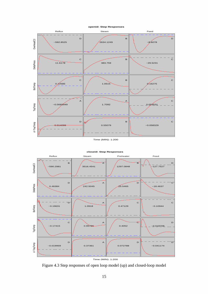
For comparison, the identification results of the open loop data and the closed-loop data areshown in Figures 4.3, 4.4 and 4.5. Note that the tray temperature TrayTemp is identified as anintegral process and the models of its derivative are shown. One can see that the quality ofclosed-loop model is higher than that of open loop model according to upper error bounds.The difference can also be seen using the process knowledge. For example, the gains betweenthe reflux and both top and bottom temperatures should be negative. The closed-loop modelcorrectly determines these. However, the gain of the open loop model is positive for thebottom temperature and is nearly zero for the top temperature. The model fit of the closed-loop model is slightly better that that of the open-loop data. The difference is partly due to thedifferent operation range and partly due to uncertainty caused by disturbance and/ornonlinearity.

Due to the change of feed flow during the closed-loop test, the usable data for identification isless than desired. Fortunately, the model from this very short test period is good enough forcontrol. This shows the accuracy of parametric models.

0 1000 2000 3000

−10

−5

0

5

Ref

lux

MV signals, open loop test

0 1000 2000 3000

−10

−5

0

5

Ref

lux

MV signals, closed−loop test

0 1000 2000 3000

−5

0

5

Ste

am

0 1000 2000 3000

−5

0

5

Ste

am

0 1000 2000 3000

−10

0

10

Pre

heat

er

0 1000 2000 3000

−10

0

10

Pre

heat

er

0 1000 2000 3000

−4

−2

0

2

4

Fee

d

Samples0 1000 2000 3000

−4

−2

0

2

4

Fee

d

Samples

Figure 4.1 MV plots of the open loop test and closed-loop test. The data are normalised bysubtracting their mean values and by dividing by some factors. For each MV, the same scaling

factor is used for both open loop test and closed-loop test.

14

0 1000 2000 3000

0

2

4O

verh

eadC

3CV signals, open loop test

0 1000 2000 3000

0

2

4

Ove

rhea

dC3

CV signals, closed−loop test

0 1000 2000 3000−1

0

1

2

Del

taP

ress

0 1000 2000 3000−1

0

1

2

Del

taP

ress

0 1000 2000 3000−4−2

02

Bot

Tem

p

0 1000 2000 3000−4−2

02

Bot

Tem

p

0 1000 2000 3000−2

024

Top

Tem

p

0 1000 2000 3000−2

024

Top

Tem

p

0 1000 2000 3000−2

0

2

4

Tra

yTem

p

Samples0 1000 2000 3000

−2

0

2

4

Tra

yTem

p

Samples

Figure 4.2 CV plots of the open loop test and closed-loop test. The data are normalised bysubtracting their mean values and by dividing by some factors. For each CV, the same scaling

factor is used for both open loop test and closed-loop test.

15

Reflux

Over

head

C3

−592.8525

D

Steam

2634.1249

B

Feed

−8.6078

D

Delta

Pres

s

11.6178

C

383.759

B

−29.5231

C

BotT

emp

0.12585

C

1.0515

B

0.16275

C

TopT

emp

−0.0069949

A

1.7092

A

0.059531

C

d−Tr

ayTe

mp

0.014099

D

0.55079

B

−0.058329

C

openid: Step Responses

Time (MIN): 1:200

Reflux

Overh

eadC

3

−590.2981

B

Steam

3516.4541

A

Preheater

1297.0848

B

Feed

−127.7527

D

Delta

Pres

s

0.46384

D

242.5045

A

25.5465

D

−18.4637

C

BotTe

mp

−0.19631

D

1.0918

A

0.47129

C

−0.10944

C

TopT

emp

−0.17415

C

0.95786

A

0.4052

C

−0.018708

D

d−Tr

ayTe

mp

−0.019959

D

0.37361

A

0.072788

D

−0.041174

D

closeid: Step Responses

Time (MIN): 1:200

Figure 4.3 Step responses of open loop model (up) and closed-loop model

16

Reflux Ov

erhea

dC3

−562.4309

D

Steam

2855.0308

B

Feed

−41.0974

D

Delta

Pres

s

20.2271

C

442.8802

B

−29.8915

C

BotTe

mp

0.18735

C

1.2357

B

0.16493

C

TopT

emp

0.023416

A

1.8434

A

0.085283

C

d−Tr

ayTe

mp

0.02465

D

0.53511

B

−0.054227

C

openid: Frequency Responses (solid) & Error Bounds

Frequency (rad/MIN): (LOG) 0.000314:3.14

Reflux

Overh

eadC

3

−589.4091

B

Steam

3458.7164

A

Preheater

1246.8705

B

Feed

−143.0344

D

Delta

Pres

s

−3.1146

D

238.1602

A

30.5064

D

−15.4426

C

BotTe

mp

−0.21724

D

1.0357

A

0.51006

C

−0.13884

C

TopT

emp

−0.15857

C

0.79818

A

0.40014

C

0.0069508

D

d−Tr

ayTe

mp

−0.018277

D

0.35552

A

0.058949

D

−0.045548

D

closeid: Frequency Responses (solid) & Error Bounds

Frequency (rad/MIN): (LOG) 0.000314:3.14

Figure 4.4 Frequency responses and error bounds of open loop and closed-loop models

17

Error%

Error%

Error%

Error%

Error%

18.1242

44.365

19.6131

22.681

64.9077

0 200 400 600 800 1000 1200 1400 1600

Time (MIN)

0

1000

2000

3000

4000

5000

6000

Overh

eadC

3

2750

2800

2850

2900

2950

3000

3050

Delta

Pres

s

80

81

82

83

84

BotTe

mp

−11

−10

−9

−8

TopT

emp

−0.5

0

0.5

d−Tra

yTem

p

openid: Model Fit, CVs (solid) & Simulated CVs

Error%

Error%

Error%

Error%

Error%

36.7326

13.5747

19.1112

23.0571

48.8301

0 200 400 600 800 1000 1200 1400 1600 1800 2000

Time (MIN)

0

2000

4000

6000

8000

10000

Overh

eadC

3

2600

2700

2800

2900

Delta

Pres

s

80

81

82

83

84

BotTe

mp

−11

−10

−9

−8

TopT

emp

−0.6

−0.4

−0.2

0

0.2

0.4

0.6

d−Tra

yTem

p

closeid: Model Fit, CVs (solid) & Simulated CVs

Figure 4.5 Model fit of open loop model (up) and closed-loop model

18

5 Conclusions and PerspectivesIn this work we have studied multivariable and closed-loop identification for use in MPC. TheASYM method is introduced to solve the problem. An industrial application is reported. Wehave shown that closed-loop tests have many advantages over open-loop tests. Whencomparing to the conventional open-loop step test approach, the following improvementshave been made by the ASYM method:

• The model quality is higher due to well-designed test, the use of parametric models andability to keep the process in a linear range.

• The disturbance to uint operation is much smaller, due to closed-loop control andencouraged operator intervention when necessary.

• The cost of identification is significantly reduced. Reduction of both test time and dataanalysis time by 70% can be realised. The method requires less user knowledge andexperience on identification.

A powerful and efficient identification method can make MPC economically feasible for moreprocess units.

From application point of view, the next logical step is to use full closed-loop test with anMPC controller online. The identified models can be used for MPC controller diagnosis andmaintenance. When sufficient industrial experience of closed-loop identification is obtained, itwould be natural to try adaptive MPC. Closed-loop identification of nonlinear models can bevery useful for difficult processes such as high purity distillation columns and more researchis needed for this challenging topic.

ReferencesCutler, C.R. and R.B. Hawkins (1988). Application of a large predictive multivariable

controller to a hydrocracher second stage reactor. Proceedings of American ControlConference, pp. 284-291.

Gustavsson I., L. Ljung and T. Söderström (1977). Identification of processes in closed loop— identifiability and accuracy aspects. Automatica, Vol. 13, pp. 59-75.

Hjalmarsson, H., M. Gevers, F. de Bruyne (1996). For model-based control design, closed-loop identification gives better performance. Automatica, Vol. 32, No. 12, pp. 1659-1673.

Jacobsen, E.W. (1994). Identification for Control of Strongly Interactive Plants. Paper 226ah,AIChE Annual Meeting, San Francisco.

Jansson, M. and B. Wahlberg (1996). On consistency of subspace system identificationmethods.

Koung, C.W. and J.F. MacGregor (1993). Design of identification experiments for robustcontrol. A geometric approach for bivariate processes. Ind. Eng. Chem. Res., Vol. 32, pp.1658-1666.

Larimore, W.E. (1990). Canonical variable analysis in identification, filtering and adaptivecontrol. Proceedings of 29th IEEE Conference on Decision and Control, Honolulu,Hawaii, pp. 596-604.

Ljung, L. (1985). Asymptotic variance expressions for identified black-box transfer functionmodels. IEEE Trans. Autom. Control, Vol. AC-30, pp. 834-844.

Ljung. L. (1987). System Identification: Theory for the User. Prentice-Hall, Englewood Cliffs,N.J.

19

Ljung, L. and Z.D. Yuan (1985). Asymptotic properties of black-box identification of transferfunctions. IEEE Trans. Autom. Control, Vol. AC-30, pp.514-530.

Qin, S.J. and T.A. Badgwell (1996). An overview of industrial model predictive controltechnology, Internet: www.che.utexas.edu/~qin/cpcv/cpcv14.html.

Richalet, J. (1993). Industrial applications of model based predictive control. Automatica,Vol. 29, No. 5, pp. 1251-1274.

Tjärnström, F. and L. Ljung (1999). L2 model reduction and variance reduction. Report LiTH-ISY-R-2158, Department of Electrical Engineering, Linköping University, June 1999.

van den Hof, P.M.J. (1997). Closed-loop issues in system identification. In Proceedings of the11th IFAC Symposium on System Identification, Fukuoka, Japan, Vol. 4, pp. 1651-1664.

Van Overschee, P. and B. De Moor (1994). N4SID: subspace algorithms for the identificationof combined deterministic-stochastic systems. Automatica, Vol. 30, No. 1, pp. 75-93.

Verhaegen, M. (1994). Identification of the deterministic part of MIMO state space modelsgiven in innovations form from input-output data. Automatica, Vol. 30, No. 1, pp. 61-74.

Wahlberg, B. (1989). Model reduction of high-order estimated models: the asymptotic MLapproach. Int. J. Control, Vol. 49, No. 1, pp. 169-192.

Zhu, Y.C. (1989). Black-box identification of MIMO transfer functions: asymptotic propertiesof prediction error models. Int. J. Adaptive Control and Signal Processing, Vol. 3, pp.357-373.

Zhu, Y.C. (1998). Multivariable process identification for MPC: the asymptotic method andits applications. Journal of Process Control, Vol. 8, No. 2, pp. 101-115.

Zhu, Y.C. and T. Backx (1993). Identification of Multivariable Industrial Processes: forSimulation, Diagnosis and Control. Springer-Verlag, London.

Zhu, Y.C. and X.H. Ge (1997). Tai-Ji ID: automatic system identification package for modelbased process control. Journal A, Vol. 38, No. 3, pp 42-45.

Zhu, Y.C. and P. van den Bosch (1999). A simple closed-loop test design formula for internalmodel control. Submitted to Automatica.

Zhu, Y.C., E. Eduardo, F. Butoyi and F. Cortes (1999). Parametric versus nonparametricmodels in industrial process identification for MPC. To appear in HydrocarbonProcessing.