Multiscale stochastic preconditioners in non-intrusive spectralprojection

A. Alexanderian,1 O.P. Le Maıtre,2 H.N. Najm,3 M. Iskandarani,4 O.M. Knio1

1Department of Mechanical EngineeringJohns Hopkins University

Baltimore, MD 21218

2LIMSI-CNRSBP 133, Bt 508

F-91403 Orsay Cedex, France

3Sandia National LaboratoriesLivermore, CA 94551

4Rosenstiel School of Marine and Atmospheric ScienceUniversity of Miami

Miami, FL 33149-1098

Suggested Running Head: Multiscale stochastic preconditioners

Corresponding Author: Omar M. KnioDepartment of Mechanical EngineeringJohns Hopkins UniversityBaltimore, MD 21218

Phone: (410) 516-7736Fax: (410) 516-7254Email: knio@jhu.edu

Submitted to: Journal of Scientific ComputingDecember 2010

1

Abstract

A preconditioning approach is developed that enables efficient polynomial chaos (PC) representa-tions of uncertain dynamical systems. The approach is based on the definition of an appropriatemultiscale stretching of the individual components of the dynamical system which, in particular,enables robust recovery of the unscaled transient dynamics. Efficient PC representations of thestochastic dynamics are then obtained through non-intrusive spectral projections of the stretchedmeasures. Implementation of the present approach is illustrated through application to a chem-ical system with large uncertainties in the reaction rate constants. Computational experimentsshow that, despite the large stochastic variability of the stochastic solution, the resulting dynamicscan be efficiently represented using sparse low-order PC expansions of the stochastic multiscalepreconditioner and of stretched variables. The present experiences are finally used to motivateseveral strategies that promise to yield further advantages in spectral representations of stochasticdynamics.

2

1 Introduction

Physical systems involving multiple variables changing dynamically over time are often modeled bysystems of differential equations. In practice, the values of model parameters are not known exactly,and are best modeled by random variables. This gives rise to dynamical systems with random pa-rameters. When studying such systems, one often aims to compute the evolution of the stochasticmodel variables, particularly to construct a statistical characterization of these variables over time.Straightforward Monte Carlo approaches, which involve simulating the random dynamical systemwith a large number of realizations of the model parameters, are too costly when working with dy-namical systems which are computationally expensive to solve; this in turn, motivates developmentof more efficient computational approaches.

An increasingly popular class of methods for quantifying uncertainty in dynamical systemsutilizes Polynomial Chaos (PC) expansions of the model variables [12, 21]. Such methods providean approximation of model variables in terms of a (finite) spectral expansion involving randompolynomials. Once available, the spectral expansion can be readily used to efficiently approximatethe distribution of the model components over time, with substantially smaller computational effortcompared to Monte Carlo sampling.

There are two major approaches for computing the spectral coefficients in a PC expansion,the Galerkin method and the so-called non-intrusive methods. The Galerkin method involvesreformulating the original random dynamical system, through its Galerkin projection onto theapproximation space spanned by the PC basis [12, 21]. One then has to solve a large system ofdeterministic differential equations for the time evolution of the PC coefficients. In contrast, thenon-intrusive methods share the common characteristic of not requiring the reformulation of theoriginal dynamical system, but aim to approximate the PC coefficients by reusing deterministicsolvers. Within this paradigm, different types of non-intrusive methods have been proposed whichcan be distinguished according to means used to obtain or approximate the PC coefficients. Existingalternatives include the non-intrusive spectral projection (NISP), the collocation method (CM),and regression-like approaches. In the NISP method, the PC coefficients are obtained based onan L2-projection of the model variables onto the space spanned by the PC basis [21, 37]. TheCM considers the PC basis as a set of interpolants and defines the PC coefficients as interpolationcoefficients [35, 28, 44, 3]. Finally, in regression-like approaches, the PC coefficients are obtainedfrom the solution of a minimization problem, namely of the distance between the spectral expansionand a set of observations for the model variables [4].

In general, PC methods face the so-called curse of dimensionality. In the context of non-intrusivemethods, this phenomenon manifests itself by the rapid increase in the number of deterministicrealizations needed for adequate determination of the PC coefficients. This limitation has motivatedmany research efforts in the past years towards complexity reduction, and great progress has beenachieved through the introduction of sparse tensorization and sparse grid techniques [17, 16, 10, 9,26].

In addition to the issue of dimensionality, a well-known difficulty that occurs with time-dependentdynamical systems concerns the broadening of the spectrum of the PC representation over time.This in turns makes it difficult to approximate model variables via fixed-order PC expansions and toselect a truncation order that remains suitable over the entire integration horizon. The underlyingdifficulty is that different realizations of the random solution trajectory fail to stay in phase as timeprogresses. In the context of chemical systems, for instance, some realizations can reach equilib-rium very quickly, while others can exhibit a transient behavior over substantially larger timescales.This decorrelation of trajectories entails the excitation of higher-order modes in a straightforwardPC representation of the model variables over time. Therefore, the corresponding PC expansions

3

require a large number of terms for a reasonably accurate approximation of the stochastic behavior.The effect of such issues has been observed for example in [36]. In Section 4.3, we will see fur-ther examples illustrating this phenomenon. Within the Galerkin framework, the approximation ofstochastic dynamics having dependence on random model parameter has given birth to alternativetechniques based on expansion over piecewise (local) polynomial bases [30, 22, 24, 40, 41], as wellas multi-resolution schemes [25, 31]. Although they enable propagation of uncertainty into systemswith complex dynamics, these advanced methods mitigate but do not address the present issue ina satisfactory fashion, as they merely reduce the computational effort by dynamically adapting theapproximation basis, which nevertheless continues to grow and eventually becomes very large [29].In contrast, the objective of the present paper is to introduce suitable transformations of the modelvariables in such a way that a low-order spectral PC basis remains suitable for arbitrarily largetimes.

In [23], the authors proposed the method of asynchronous integration in the context of theGalerkin method. Targeting random dynamical systems having almost surely stable periodic tra-jectories, the key idea of the approach is that, assuming a smooth dependence of the limit-cyclewith regard to the uncertain system parameters, the random trajectory can be expanded on a loworder PC basis provided that one can maintain the process nearly in phase. This is achieved byintroducing a time rescaling that depends on the random parameters.

Inspired by the work in [23], we presently explore an alternative stochastic preconditioningapproach, in the context of non-intrusive methods. The method addresses the issue of wideningspectra by introducing a global multiscale linear or affine transformation of the solution variables soas to synchronize realizations, and consequently control their variance and PC spectrum. Comparedto the developments in [23], we relax the assumption of periodic dynamics, and exploit the non-intrusive character of the method to introduce random scaling parameters for each of the systemvariables. The method, which is illustrated for stiff chemical systems, is outlined in Section 3. Indoing so, we exclusively rely on a non-intrusive formalism based on NISP. However, we emphasizethe fact that extension to other type of non-intrusive methods is immediate. The basic idea behindthe method is to work with transformed variables in scaled time which are in phase and havecontrolled spectra, i.e. the transformed variables have tight low order PC representations which canbe computed with a limited number of realizations. Subsequently, the distribution of the originalvariables can be easily recovered, from that of transformed ones, through a sampling strategy.

The structure of the paper is as follows. In Section 2, we introduce the basic notation andthe background ideas needed throughout the paper. In particular, we provide a brief overview ofthe PC expansion of square integrable random variables, dynamical systems with random inputs,and the classical NISP method. Section 3 focuses on our proposed preconditioning method forNISP. We start by introducing the random scaling parameters and define the associated scaledvariables. Next, we highlight the projection of the scaled variables onto the PC basis, and outline therecovery of the original random model variables from their stretched counterparts. Implementationof preconditioned NISP is illustrated for the case of a stiff chemical system that is introduced inSection 4. The system consists of a simplified mechanism for supercritical water oxidation. Itsselection is motivated by prior analysis of similar systems [36, 25], which had revealed complexdependence of the dynamics on random rate parameters. Computational experiments are thenpresented in Section 5 where we demonstrate projection of the stretched variables and the recoveryof the original variables. The computations are further analyzed in Section 6 in light of errorand convergence estimates, and in Section 7 where we discuss an extension of the preconditioningframework introduced earlier. A brief summary is provided in Section 8 together with a discussionof possible generalizations.

4

2 Background

In this section we fix the notation and collect background results used in the rest of the paper. Inwhat follows (Ω,F , µ) denotes a probability space, where Ω is the sample space, F is an appropriateσ-algebra on Ω, and µ is a probability measure. A real-valued random variable ξ on (Ω,F , µ) is anF/B(R)-measurable mapping ξ : (Ω,F , µ) → (R,B(R)), where B(R) denotes the Borel σ-algebraon R. The space L2(Ω,F , µ) denotes the Hilbert space of real-valued square integrable randomvariables on Ω.

For a random variable ξ on Ω, we write ξ ∼ N (0, 1) to mean that ξ is a standard normalrandom variable and we write ξ ∼ U(a, b) to mean that ξ is uniformly distributed on the interval[a, b]. We use the term iid for a collection of random variables to mean that they are independentand identically distributed. The distribution function [15, 43] of a random variable ξ on (Ω,F , µ)is given by Fξ(x) = µ(ξ ≤ x) for x ∈ R.

2.1 Polynomial Chaos

In this paper, we consider dynamical systems with finitely many random parameters, parameterizedby a finite collection of real-valued iid random variables ξ1, . . . , ξM on Ω. We let V = σ(ξiM1 ) be theσ-algebra generated by ξ1, . . . , ξM and, disregarding any other sources of uncertainty, work in thespace (Ω,V, µ). By Fξ denote the joint distribution function of the random vector ξ = (ξ1, . . . , ξM )T .Note that since the ξj are iid Fξ(x) =

∏Mj=1 F (xj) for x ∈ RM . Let us denote by Ω∗ ⊆ RM the

image of Ω under ξ, Ω∗ = ξ(Ω), and by B(Ω∗) the Borel σ-algebra on Ω∗. It is often convenientto work in the image probability space (Ω∗,B(Ω∗), Fξ) instead of the abstract probability space(Ω,V, µ). We denote the expectation of a random variable X : Ω∗ → R by 〈X〉 =

∫Ω∗ X(s) dFξ(s).

The space L2(Ω∗,B(Ω∗), Fξ) is endowed with the inner product (·, ·) : L2(Ω∗)× L2(Ω∗)→ R givenby (X,Y ) =

∫Ω∗ X(s)Y (s) dFξ(s) = 〈XY 〉.

In the case ξiiid∼ N (0, 1), any X ∈ L2(Ω∗,B(Ω∗), Fξ) admits an expansion of form,

X =∞∑k=0

ckΨk, (1)

where Ψk∞0 is a complete orthogonal set consisting of M -variate Hermite polynomials [1], andthe series converges in L2(Ω∗,B(Ω∗), Fξ). The expansion (1) is known as the (Wiener-Hermite)polynomial chaos expansion [42, 6, 14, 21] of U . In practice, the Wiener-Hermite expansionis most useful when the model parameters are parameterized by normally distributed randomvariables. In cases where the sources of uncertainty follow other distributions, it is convenient toadopt alternative parameterizations and polynomial bases. For example, in the case ξi

iid∼ U(−1, 1),we will use M -variate Legendre polynomials for the basis Ψk∞0 , and the expansion in (1) is aGeneralized Polynomial Chaos [45] expansion of U .

Finally, in practical computations, we will be approximating X(ξ) with a truncated series,

X(ξ) .=P∑k=0

ckΨk(ξ), (2)

where P is finite and depends on the truncation strategy adopted. In the following, we considertruncations based on the total degree of the polynomials in the series, such that P depends of the

stochastic dimension M and expansion “order” p according to: 1 + P =(M + p)!M !p!

, where p refers

to the largest polynomial degree in the expansion.

5

2.2 Uncertain dynamical systems

Consider the autonomous ODE system, X = F (X),X(0) = X0,

(3)

where the solution X of the system is a function X : [0, Tfin]→ Rn, with

X(t) = [X1(t), . . . , Xn(t)]T .

We consider the case of parametric uncertainty in the source term, i.e. F = F (X, ξ). Thus, thesolution of (3) is a stochastic process,

X : [0, Tfin]× Ω∗ → Rn.

We can rewrite (3) more precisely asX(t, ξ) = F

(X(t, ξ), ξ

)X(0, ξ) = X0, a.s.

(4)

To capture the distribution of Xi(t, ξ) at a given time, we will rely on the truncated PCexpansion,

Xi(t, ξ) =P∑k=0

cik(t)Ψk(ξ),

where the time-dependent coefficients cik(t) are to be computed non-intrusively, as outlined in thefollowing section.

2.3 Non Intrusive Spectral Projection

Let us focus on a generic component of the uncertain dynamical system at a fixed time t ∈ [0, Tfin]and simply denote this by X. As mentioned in the introduction, non-intrusive methods aim atcomputing the PC coefficients in the finite expansion (2) via a set of deterministic evaluations ofX(ξ) for specific realizations of ξ. The NISP method, that will be used in throughout this paper,defines the expansion coefficients ck in the expansion of X(ξ) as the coordinates of its orthogonalprojection on the space spanned by the ΨkP0 . Observe that since ΨkP0 form an orthogonalsystem we have (cf. for example [32]):(

X −P∑l=0

clΨl,Ψk

)= 0, k = 0, . . . , P.

Therefore,

(X,Ψk) =

(P∑l=0

clΨl,Ψk

)=

P∑l=0

cl (Ψl,Ψk) = ck (Ψk,Ψk) , (5)

so that the coefficient ck is given by

ck =〈XΨk〉⟨

Ψ2k

⟩ . (6)

6

In the case of Hermite or Legendre polynomials, the moments⟨Ψ2k

⟩in (6) can be computed ana-

lytically and hence, the determination of coefficients ck amounts to the evaluation of the moments〈XΨk〉. We note that

〈XΨk〉 =∫

Ω∗X(s)Ψk(s) dFξ(s), k = 0, . . . , P.

leading to the evaluation of a set of P + 1 integrals over Ω∗ ⊆ RM to obtain the set of projectioncoefficients. These integrals are classically discretized as finite sums of the form

∫Ω∗X(s)Ψk(s) dFξ(s) =

Nq∑j=1

wjX(ξj)Ψk(ξj) +Rk,Nq(X), (7)

where ξj ∈ Ω∗ and wj are the nodes and weights of an appropriate quadrature formula, andRk,Nq(X) is the integration error. Note that the same set of nodes is used to compute all thecoefficients ck, so the complexity of NISP scales with Nq, the number of nodes where one hasto compute X. Therefore, the challenge is to design quadrature formulae yielding the lowestintegration error for the minimal number of nodes. In general, this is a difficult problem, and oneoften proceeds by tensorization of one-dimensional quadrature rules. Considering a 1-D quadraturerule with n1 nodes, its full tensorization gives a M -variate formula having Nq = nM1 nodes, showingthat this approach is limited to low M . This exponential scaling with M is often referred to as thecurse of dimensionality. The latter can be significantly tempered by relying on sparse tensorizationsof sequences of 1-D formulae using Smolyak’s formula [38], which leads to sparse-grid integrationtechniques [11, 33, 34].

Irrespective of the formula considered for the computation of the ck, the set of integration nodescomprise what we call the NISP sample and denote by

S = ξjNq

j=1 ⊂ Ω∗.

Thus, to evaluate (7) we need to compute X(ξq) for all ξq ∈ S. Let the matrix Π = (Πkj),k = 0, . . . , P and j = 1, . . . , Nq be given by

Πk,j =wjΨk(ξj)⟨

Ψ2k

⟩ .

We call the matrix Π the NISP projection matrix. If we denote by x the vector with coordinatesxj = X(ξj), then the vector c = [c0, . . . , ck]T of the spectral coefficients in (6) is given by thematrix vector product

c = Πx,

or in components,

ck =Nq∑j=1

Πkjxj =Nq∑j=1

ΠkjX(ξj), k = 0, . . . , P.

Going back to the original problem of projecting the n components of the solution X(t, ξ) to theuncertain dynamical system (4), we observe that the projection matrix Π is time independentand the same for all the components. As a result, the NISP projection of X(t, ξ) requires theresolution of the deterministic dynamics corresponding to X(t, ξq), for each ξq ∈ S. We outlinethe calculation of PC coefficients of X(t, ξ) .=

∑Pk=0 ck(t)Ψk(ξ) over time in Algorithm 1.

7

Algorithm 1 The classical NISP algorithmNt = Tfin/∆t number of time stepsNq = |S| number of elements of Sfor j = 1 to Nq do

Compute X(i∆t, ξj), i = 0, . . . , Nt deterministic solvefor i = 0 to Nt doti = i∆tfor k = 0 to P dock(ti) = ck(ti) + ΠkjX(ti, ξj) NISP sum

end forend for

end for

3 Preconditioned Non Intrusive Spectral Projection

When applying NISP (or any non-intrusive method), the computational complexity mainly dependson the number of sampling points needed to construct the approximation. This in turn is functionof the complexity of the distribution of the random quantity one seeks to approximate, which as faras NISP is concerned, relates to the polynomial order needed for sufficient accuracy. As a result,the higher the polynomial order needed to obtain a suitable representation, the larger will be theNISP sample required. Therefore, preconditioning the random quantity so as to reduce the order ofthe PC expansion is of practical interest. This is the essential idea proposed in the present paper,where we pursue this goal through the appropriate transformation of an original time-dependentrandom vector X into a new one Y having a tight sparse PC expansion requiring less efforts tobe projected. Such a procedure generally involves three distinct steps, namely the definition of thetransformation (Section 3.1), the projection of the transformed variables (Section 3.2), and finallythe recovery of the original variable (Section 3.3) for the purpose of sampling and analysis.

Taking advantage of the non-intrusive character of the proposed method, the preconditioning isperformed separately for each component, Xi, of the system. Therefore, for convenience, we dropin this section the superscript i and consider a generic component X and its transform Y . Sincein the present applications we will restrict ourselves to scaling-type transformations, we shall oftenrefer to the transformed variable Y as the scaled variable.

3.1 Variable transformations

Recall that the state variable X is a stochastic process, X : [0, Tfin]× Ω∗ → R. We introduce thetransformed variable Y = Y (τ, ξ) that depends on a scaled time τ . The scaled time τ = τ(t, ξ) isdefined through,

τ(t, ξ) =t

t(ξ), t ∈ [0,+∞), (8)

where t : Ω∗ → (0,∞) is a random variable which we call the time scaling factor. We assume thatthere exist positive constants κ1 < κ2 such that

κ1 ≤ t(ξ) ≤ κ2, for almost all ξ ∈ Ω∗.

In general, we define the scaled variable Y by

Y (τ(t, ξ), ξ) = Φ[X(t, ξ)].

8

where Φ is an invertible mapping on L2(Ω∗). In the present work, we will mainly focus on the caseof linear scaling defined through

Φ[X(t, ξ); c] =1c(ξ)

X(t, ξ), (9)

where c : Ω∗ → (0,∞) is an amplitude scaling factor ; we assume that there exist positive constantsν1 and ν2 that are independent of ξ and

ν1 ≤ c(ξ) ≤ ν2, for almost all ξ ∈ Ω∗. (10)

Note that (10) ensures that c ∈ L∞(Ω∗) ⊂ L2(Ω∗); moreover, we have 1/c ∈ L∞(Ω∗) and sinceX(t, ·) ∈ L2(Ω∗) it follows that Φ[X(t, ·); c] ∈ L2(Ω∗), for every t ∈ [0, Tfin]. In the case whereX(t, ξ) is positive valued, as is the case for chemical species concentrations, we may also considerlog-linear scaling,

Φ[X(t, ξ); c] = log(

1c(ξ)

X(t, ξ)). (11)

An advantage of the log-linear scaling is in preserving positivity of the recovered state variables,as further discussed below. Moreover, since we will ultimately approximate the scaled variableswith their PC expansions, sometimes the log-linear scaling may result in a better behaved PCrepresentations for the scaled variables.

Remark 3.1 One may consider more general types of transformations Φ[X] and the scalingmethod introduced above can be seen as a particular instance of a broader class of preconditioners.An affine transformation is later discussed, though more general mappings are yet to be explored.

Remark 3.2 A fundamental question that we will be concerned with is: How to choose the scalingfactors t and c so that the scaled variable Y has a tight sparse PC representation that can beefficiently obtained on the basis of a coarse non-intrusive sampling? In addition, we will eventuallyhave to approximate t and c via PC expansions, and hence it is of practical concern that thesescaling factors themselves have controlled PC representations. In the current work, we base thisselection on the observed behavior of the state variables of the chemical model in our study, seeSection 4. A general strategy for obtaining suitable scaling factors (and ideally selecting moregeneral transformations) remains an open issue, as further discussed in Section 8.

3.2 Projection of the scaled variables

Here we describe in detail the projection of the scaling factors and the scaled variables into a PCbasis.

3.2.1 Expansion of the scaling factors

We will need PC representations of the scaling factors, c and t. These expansions will be computedusing the NISP sample set S. We will assume that for each ξj ∈ S one is able to define acorresponding pair of factors (t(ξj); c(ξj)); as discussed in Section 4, the corresponding realizationX(ξj , t) is used for this purpose. The expansions of the scaling factors are

c.=

P∑k=0

ckΨk, t.=

P∑k=0

tkΨk,

9

where the expansion coefficients are computed through a classical NISP procedure:

ck =Nq∑j=1

Πk,j c(ξj), tk =Nq∑j=1

Πk,j t(ξj).

Since c and t are positive we may also consider the expansion of their logarithms. This again hasthe advantage of preserving their positivity and in some cases yielding nicer (tighter and/or sparser)PC spectra. In particular, we will project the logarithm of the normalized variables, c(ξ)/c(ξ = 0)and t(ξ)/t(ξ = 0):

log(c(ξ)c(0)

).=

P∑k=0

σkΨk, log(t(ξ)t(0)

).=

P∑k=0

θkΨk,

where

σk =Nq∑j=1

Πk,j log(c(ξj)c(0)

), θk =

Nq∑j=1

Πk,j log

(t(ξj)

t(0)

). (12)

Accordingly c and t are approximated through,

c.= c(0) exp

(P∑k=0

σkΨk

), t

.= t(0) exp

(P∑k=0

θkΨk

). (13)

In the computations below, we will use (13) to approximate c and t.

3.2.2 Scaled variable discretization

The major computational work in the method involves the non-intrusive projection of the trans-formed variable Y (τ(t, ξ), ξ) = Φ

[X(t, ξ); c

]to get its PC representation. This calls for time

discretization. Owing to the assumed properties of the time scaling in (8), for every t ∈ [0,+∞),τ(t, ·) ∈ [0,+∞) almost surely. Moreover, for a given (t′, ξ) ∈ [0,+∞) × Ω∗, there corresponds an(unscaled) time t given by t = t′ × t(ξ) and we have that

Y (t′, ξ) = Φ[X(t′ × t(ξ), ξ

); c].

This allows us to discretize the transformed variable Y on a fixed deterministic grid of times t′ inthe scaled space. With the slight abuse of notation where there is no confusion between τ and t′,the PC expansion sought is then expressed as

Y (τ, ξ) .=P∑k=0

Yk(τ)Ψk(ξ) ≈ Φ[X(τ × t(ξ), ξ); c

], (14)

where the PC coefficients Yk(τ) are to be computed on a fixed grid of scaled times τ . Specifically,given ∆τ > 0 and defining τl

.= l∆τ , l = 0, 1, . . . the NISP projection of the k-PC mode of Y wouldbe

Yk(τl) =Nq∑j=1

Πk,jΦ[X(τl × t(ξj), ξj); c

]. (15)

10

3.2.3 Preconditioned projection algorithm

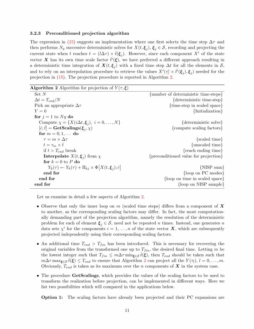
The expression in (15) suggests an implementation where one first selects the time step ∆τ andthen performs Nq successive deterministic solves for X(t, ξj), ξj ∈ S, recording and projecting thecurrent state when t reaches t = (l∆τ) × t(ξj). However, since each component Xi of the statevector X has its own time scale factor ti(ξ), we have preferred a different approach resulting ina deterministic time integration of X(t, ξj) with a fixed time step ∆t for all the elements in S,and to rely on an interpolation procedure to retrieve the values Xi(τ il × ti(ξj), ξj) needed for theprojection in (15). The projection procedure is reported in Algorithm 2.

Algorithm 2 Algorithm for projection of Y (τ, ξ)Set N number of deterministic time-steps∆t = Tend/N deterministic time-stepPick an appropriate ∆τ time-step in scaled spaceY = 0 Initializationfor j = 1 to Nq do

Compute χ = X(i∆t, ξj), i = 0, . . . , N deterministic solve[c, t] = GetScalings(ξj , χ) compute scaling factorsfor m = 0, 1, . . . doτ = m×∆τ scaled timet = τm × t unscaled timeif t > Tend break reach ending timeInterpolate X(t, ξj) from χ preconditioned value for projectionfor k = 0 to P doYk(τ)← Yk(τ) + Πkj × Φ

[X(t, ξj); c

]NISP sum

end for loop on PC modesend for loop on time in scaled space

end for loop on NISP sample

Let us examine in detail a few aspects of Algorithm 2.

• Observe that only the inner loop on m (scaled time steps) differs from a component of Xto another, as the corresponding scaling factors may differ. In fact, the most computation-ally demanding part of the projection algorithm, namely the resolution of the deterministicproblem for each of element ξj ∈ S, need not be repeated n times. Instead, one generates ndata sets χi for the components i = 1, . . . , n of the state vector X, which are subsequentlyprojected independently using their corresponding scaling factors.

• An additional time Tend > Tfin has been introduced. This is necessary for recovering theoriginal variables from the transformed one up to Tfin, the desired final time. Letting m bethe lowest integer such that Tfin ≤ m∆τ minξ∈S t(ξ), then Tend should be taken such thatm∆τ maxξ∈S t(ξ) ≤ Tend to ensure that Algorithm 2 can project all the Y (τl), l = 0, . . . ,m.Obviously, Tend is taken as its maximum over the n components of X in the system case.

• The procedure GetScalings, which provides the values of the scaling factors to be used totransform the realization before projection, can be implemented in different ways. Here welist two possibilities which will compared in the applications below.

Option 1: The scaling factors have already been projected and their PC expansions are

11

known at this stage. Accordingly, GetScalings simply returns the values c and t givenby the respective PC expansions in (13) evaluated at ξ = ξj .

Option 2: The PC expansions of the scaling factors are not known at this stage. In thiscase, GetScalings returns values c and t which are the scaling factors determined fromthe analysis of the current realization dynamics, that is using the deterministic timeseries in χ (see Section 4).

The first option supposes that the scaling factors have been previously projected, possibly us-ing a different set of NISP nodes. This approach thus seems to waste computational resources,because, as discussed above, the projection of the scaling factors requires the simulation ofthe whole system for each point in S to determine c(ξj) and t(ξj) used in the projectionthrough (12). This was not the case for the example proposed in this paper, as we couldafford to store simulation results for every ξj ∈ S, and readily reuse them in Algorithm 2with Option 1. However, this luxury may not be an option for larger S and/or more com-plex systems. This limitation leads to considering Option 2 where the transformation of therealization uses scaling factors determined on the fly, i.e. based uniquely on the currentrealization. For this second option, we also insert in Algorithm 2 an additional step (insidethe loop on NISP points, but external to the loop on the scaled time-step) where c and t areprojected, simultaneously with Y , using t(ξj) = t and c(ξj) = c in (12). It is important toremark that, due to projection errors for the scaling factors, the two options result in differentPC expansions for the scaled variables Y . Specifically, one does not recover exactly the valuesc(ξj) and t(ξj) used in (12) when evaluating (13) at ξ = ξj , because of NISP integration andtruncation errors. When using Option 2, these differences have to be controlled, as the recov-ery procedure (to be discussed shortly) uses the PC expansions of the scaling factors to invertthe transformation. Therefore, inconsistencies in the definition of the scaling factors betweenΦ (the forward transform) and its inverse Φ−1 (the backward transform) may constitute anadditional source of error.

• For the interpolation step we use a simple linear interpolation scheme to approximate X(·, ξj)between elements in χ. Specifically, the interpolated value X(t, ξj) is evaluated from

X(t, ξj) = X(tl, ξj) +[X(tl + ∆t, ξj)−X(tl, ξj)

∆t

](t− tl),

where tl = l∆t is such that tl ≤ t < tl + ∆t. Note that higher order interpolation schemescould be used, but this was found unnecessary in the application presented in this paper aswe could afford to store computed solutions using sufficiently small time increments ∆t.

• We have kept the algorithm general by not specifying the transformation Φ used in computa-tion of the scaled variables. Throughout the paper, unless otherwise mentioned, we will relyon the linear scaling as defined in (9).

3.3 Recovering the original variables

We now turn to the problem of reconstructing X(t, ξ) from the transformed variable Y (τ, ξ). Theobjective is to derive an efficient procedure to resample X(t, ξ), particularly to perform variousstatistical analyses. Given t ∈ [0, Tfin] and a realization ξl ∈ Ω∗, we would like to to reconstruct thecorresponding value of X(t, ξl). Again, we focus on the treatment of a single generic componentX of X, as the generalization is immediate.

12

3.3.1 Backward transformation

The recovery amounts to the inversion of the transformation:

X(t, ξ) = Φ−1 [Y (τ(t, ξ), ξ); c(ξ)] . (16)

For the case of linear scaling, we have

X(t, ξ) = Φ−1 [Y (τ(t, ξ), ξ); c(ξ)] = c(ξ)Y (τ(t, ξ), ξ), (17)

while for the case of log-linear scaling, we have

X(t, ξ) = Φ−1 [Y (τ(t, ξ), ξ)] = c(ξ) exp(Y (τ(t, ξ), ξ)

). (18)

Of course, in practice we will approximate X by inserting the PC expansions of the scaling factorsand scaled variables in (16). Let us introduce the notation X to denote the recovered state variableX from the PC expansions of the scaled variable through the above relations. We have,

X(t, ξ) = c(ξ)∑P

k=0 Yk(τ(t, ξ))Ψk(ξ)

linear scaling,

X(t, ξ) = c(ξ)

exp(∑P

k=0 Yk(τ(ξ, t))Ψk(ξ))

log-linear scaling.(19)

3.3.2 Recovery and sampling algorithms

At a given t∗ ∈ [0, Tfin], we can sample the expansion of X(t∗, ·) in (19) to generate an approximatedistribution of X(t∗, ·) fairly efficiently. The only issue remaining is that the PC coefficients of thescaled variable Y are known on the fixed grid of scaled times τl which generally will not coincide withthe time τ(t∗, ·) in (19). Again, we rely on linear interpolation to compute the PC coefficients Ykat the needed scaled time τ . The resulting procedure for computing X is provided in Algorithm 3.Note that in Algorithm 3 the procedure GetScalings returns the values of the scaling factorsevaluated from their PC expansions (as for Option 1).

Algorithm 3 Procedure for computing X(t∗, ξ∗) at t∗ ∈ [0, Tfin] and ξ∗ ∈ Ω∗

[c, t] = GetScalings(ξ∗) compute scaling factors from PC expansionsτ∗ = t∗/t scaled timeFind τl such that τ∗ ∈ [τl, τl+1]for k = 0 to P do

Yk(τ∗) = Yk(τl) +[Yk(τl+1)− Yk(τl)

∆τ

](τ∗ − τl) Interpolate Yk(τ∗)

end for loop on PC modesCompute X(t∗, ξ∗) from (19) with τ(t∗, ξ∗) = τ∗ and c(ξ∗) = c. apply inverse transformation

Finally, the complete sampling method is immediately constructed through a Monte Carlo pro-cedure wrapped around the recovery procedure in Algorithm 3. For fixed t∗, one only has to sampleΩ∗ from the distribution Fξ to obtain a sampling of the distribution of X(t∗, ·). This is summarizedin Algorithm 4 which will be used in Section 6 to assess the efficiency of the Preconditioned NISP.

13

Algorithm 4 Algorithm for sampling X(t∗, ·) at a given t∗ ∈ [0, Tfin]Set Ns number of sample points to be generatedfor ` = 1 to Ns do

Draw at random ξ` from the distribution Fξ random sampling of Ω∗Compute X(t∗, ξ`) using procedure in Algorithm 3 recover realization value

end for loop on sample

14

4 Model problem

In this section, we describe the dynamical system that will be used to illustrate our proposedpreconditioning strategy. The system corresponds to a hydrogen oxidation problem, based on thereduced mechanism that was proposed in [35]. This problem was chosen because it is known toyield solutions with broad spectra when decomposed on PC bases [37]. Previous studies based onstochastic Galerkin projection methods showed that the solution has complex dynamics, is highlysensitive to model parameters (rate constants), and therefore requires a fine stochastic discretizationand adaptive strategies to be properly approximated [25, 29].

4.1 Stochastic model

The reduced mechanism from [35] involves the concentrations of seven species, namely [OH], [H],[H2O], [H2], [O2], [HO2], and [H2O2], whose evolution is governed by eight elementary reversiblereactions. We let kf,j and kr,j respectively denote the forward and reverse rate constant of thej-th reaction, j = 1, . . . , 8. The randomness enters the model through uncertainty in the forwardreaction rates kf,j , j = 1, . . . 8. Isothermal conditions are assumed, and the standard heats andentropies of the formation of the species are assumed deterministic. Accordingly, the equilibriumconstant constants Kc,j are deterministic, and the reverse rates are given by

kr,j = K−1c,j × kf,j (a.s.), j = 1, . . . , 8.

We further assume that the model forward reaction rates are independent uniformly-distributedrandom variables. As a result, they can be parametrized using a set of 8 IID random variables ξj ,according to

kf,j = aj + bjξj , ξj ∼ U(−1, 1), j = 1, . . . 8,

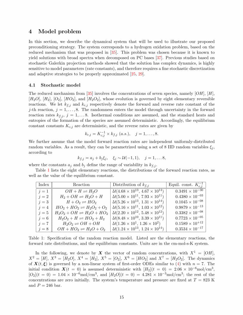
where the constants aj and bj define the range of variability in kf,j .Table 1 lists the eight elementary reactions, the distributions of the forward reaction rates, as

well as the value of the equilibrium constant.

Index Reaction Distribution of kf,j Equil. const. K−1c,j

j = 1 OH +H H2O U(4.68× 1013, 4.67× 1014) 0.3491× 10−30

j = 2 H2 +OH H2O +H U(5.00× 1011, 7.93× 1011) 0.4380× 10−03

j = 3 H +O2 HO2 U(5.26× 1013, 1.31× 1014) 0.1045× 10−08

j = 4 HO2 +HO2 H2O2 +O2 U(5.16× 1011, 1.03× 1012) 0.9879× 10−13

j = 5 H2O2 +OH H2O +HO2 U(2.20× 1012, 5.48× 1012) 0.3382× 10−08

j = 6 H2O2 +H HO2 +H2 U(8.48× 1010, 3.39× 1011) 0.7723× 10−05

j = 7 H2O2 OH +OH U(1.26× 101, 1.26× 102) 0.1589× 10+12

j = 8 OH +HO2 H2O +O2 U(1.24× 1013, 1.24× 1014) 0.3534× 10−17

Table 1: Specification of the random reaction model. Listed are the elementary reactions, theforward rate distributions, and the equilibrium constants. Units are in the cm-mol-s-K system.

In the following, we denote by X the vector of random concentrations, with X1 = [OH],X2 = [H], X3 = [H2O], X4 = [H2], X5 = [O2], X6 = [HO2] and X7 = [H2O2]. The dynamicsof X(t, ξ) is governed by a non-linear system of first-order ODEs similar to (4) with n = 7. Theinitial condition X(t = 0) is assumed deterministic with [H2](t = 0) = 2.06 × 10−6mol/cm3,[O2](t = 0) = 1.04 × 10−6mol/cm3, and [H2O](t = 0) = 4.281 × 10−3mol/cm3; the rest of theconcentrations are zero initially. The system’s temperature and pressure are fixed at T = 823 Kand P = 246 bar.

15

4.2 The sample set S

Here we briefly describe the NISP sample S we used for the purposes of computations which followin the subsequent sections. Recall that S is the set of integration nodes for evaluation of the PCcoefficients through (7). In our case, we used full tensorization of a (one-dimensional) 5-pointGauss-Legendre quadrature formula [1, 2]. If we denote by S0 the set of five Gauss-Legendre nodes,the set S is then given by

S = S0 × S0 × · · · × S0︸ ︷︷ ︸8 times

.

Thus, S has 58 = 390, 625 elements. While this may seem like a fairly large sample, in fact it isa fairly coarse sampling of the space Ω∗. Specifically, consistent with prior experiences in [25], wewill later illustrate that direct NISP using the present sample set does not lead to a suitable PCrepresentation.

4.3 Analysis of the stochastic dynamics

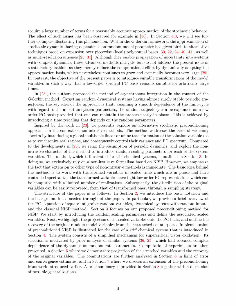
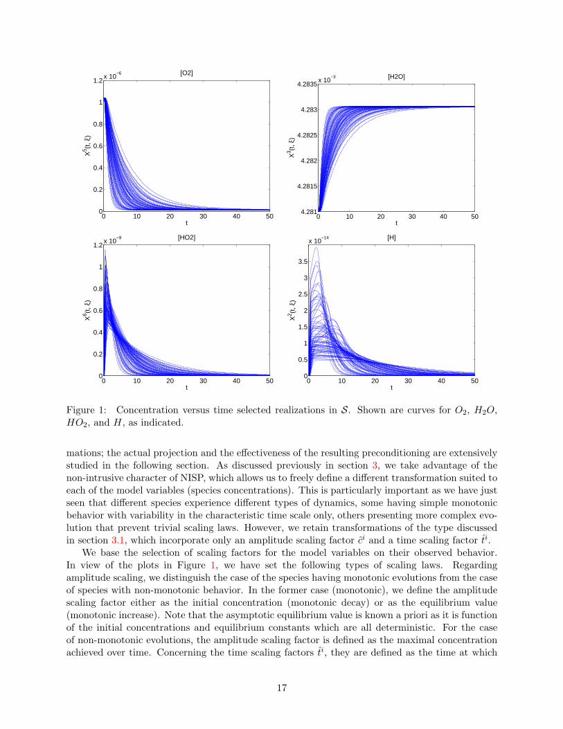
Figure 1 shows the evolution of species concentrations corresponding to deterministic realizationsof the system taken in S. Shown are the species O2, H2O, H, and HO2, which are typical; the caseof OH requires special treatment as later discussed in Section 8.

Figure 1 depicts the different types of dynamics observed for the species considered. Thecurves for O2 (top-left) indicate that for all the realizations shown the concentration decreasesmonotonically with time. Uncertainty in the model parameters only affects the decay rate of[O2](t). A similar behavior is also reported for H2 (not shown). In contrast, the case of H2O (top-right) corresponds to a monotonic increase of its concentration, which asymptotes to a deterministicequilibrium value (as must be the case since the equilibrium constants are assumed deterministic).However, the random model parameters are again seen to affect the characteristic response time of[H2O]. HO2 exhibits a more complex behavior, with a very fast initial increase in concentration,followed by a substantially slower monotonic decay. Unlike the previous cases where the randominputs were seen to modulate the response time scales, in the present case the peak amplitudes aresubstantially impacted as well. The case of H is essentially similar to HO2, although with slowerresponse time during the production stage. Also noticeable is the presence of some plateaus ofdifferent widths, during which [H] remains nearly constant before it starts to decay.

These typical dynamics underscore potential difficulties faced in direct projection of the speciesconcentrations. First, for the simplest case of monotonic dynamics, it is seen that time-scale vari-ability leads to substantial variability in the stochastic concentration at a given time. This may notresult in complex PC spectra, provided that the time-scale variability remains moderate. In fact,the occurrence of high variability in fast time-scales is frequently observed in ignition problems,which are known to be extremely challenging [31]. At any rate, it appears that an appropriate timetransformation reducing the time-scale variability would certainly help controlling the correspond-ing PC spectrum. For non-monotonic dynamics, the difficulties above are further compounded bysubstantial uncertainty in the position and amplitude of the maxima. This variability is anticipatedto lead to broad PC spectra, and consequently challenges in the representation of the stochasticsolution. For the case of H, the occurrence of plateaus of variable durations is anticipated to makethese challenges even more severe.

4.4 Scaling of the stochastic dynamics

We now propose appropriate transformations of the individual realizations in view of the PC pro-jection of the transformed signals. The objective here is simply to support our choice of transfor-

16

0 10 20 30 40 500

0.2

0.4

0.6

0.8

1

1.2x 10

−6 [O2]

t

X5 (t

, ξ)

0 10 20 30 40 504.281

4.2815

4.282

4.2825

4.283

4.2835x 10

−3 [H2O]

t

X3 (t

, ξ)

0 10 20 30 40 500

0.2

0.4

0.6

0.8

1

1.2x 10

−9 [HO2]

t

X6 (t

, ξ)

0 10 20 30 40 500

0.5

1

1.5

2

2.5

3

3.5

x 10−14 [H]

t

X2 (t

, ξ)

Figure 1: Concentration versus time selected realizations in S. Shown are curves for O2, H2O,HO2, and H, as indicated.

mations; the actual projection and the effectiveness of the resulting preconditioning are extensivelystudied in the following section. As discussed previously in section 3, we take advantage of thenon-intrusive character of NISP, which allows us to freely define a different transformation suited toeach of the model variables (species concentrations). This is particularly important as we have justseen that different species experience different types of dynamics, some having simple monotonicbehavior with variability in the characteristic time scale only, others presenting more complex evo-lution that prevent trivial scaling laws. However, we retain transformations of the type discussedin section 3.1, which incorporate only an amplitude scaling factor ci and a time scaling factor ti.

We base the selection of scaling factors for the model variables on their observed behavior.In view of the plots in Figure 1, we have set the following types of scaling laws. Regardingamplitude scaling, we distinguish the case of the species having monotonic evolutions from the caseof species with non-monotonic behavior. In the former case (monotonic), we define the amplitudescaling factor either as the initial concentration (monotonic decay) or as the equilibrium value(monotonic increase). Note that the asymptotic equilibrium value is known a priori as it is functionof the initial concentrations and equilibrium constants which are all deterministic. For the caseof non-monotonic evolutions, the amplitude scaling factor is defined as the maximal concentrationachieved over time. Concerning the time scaling factors ti, they are defined as the time at which

17

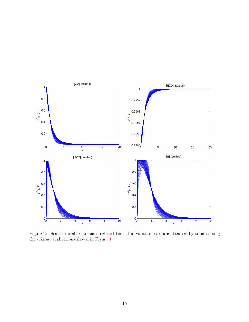
the corresponding species concentrations reaches a specific concentration value which depends onthe amplitude scaling factor selected and eventually the initial concentration. We list our choiceof (amplitude) ci and (time) ti scale factor definitions for i = 2, . . . , 7 in Table 2. Note that forXi=3,4,5 the scaling factors ci are deterministic because they depend on initial or steady-state valueswhich are deterministic in the present experiments.

Amplitude scaling Time scaling Typec2(ξ) = max

tX2(t, ξ) t2(ξ) = time for X2(t, ξ) to return to 1

2 c2(ξ) non-monotonic

c3(ξ) = limt→∞

X3(t, ξ) t3(ξ) = time for X3(t, ξ) to reach12

(X3(0) + c2(ξ)) monotonic ↑

c4(ξ) = X4(0) t4(ξ) = time for X4(t, ξ) to reach12c4(ξ) monotonic ↓

c5(ξ) = X5(0) t5(ξ) = time for X5(t, ξ) to reach12c5(ξ) monotonic ↓

c6(ξ) = maxtX6(t, ξ) t6(ξ) = time for X6(t, ξ) to return to

12c6(ξ) non-monotonic

c7(ξ) = maxtX7(t, ξ) t7(ξ) = time for X7(t, ξ) to return to

12c7(ξ) non-monotonic

Table 2: Definition of the scaling factors ci(ξ) and ti(ξ) for the transformation of the model variablesXi, i = 2, . . . , 7.

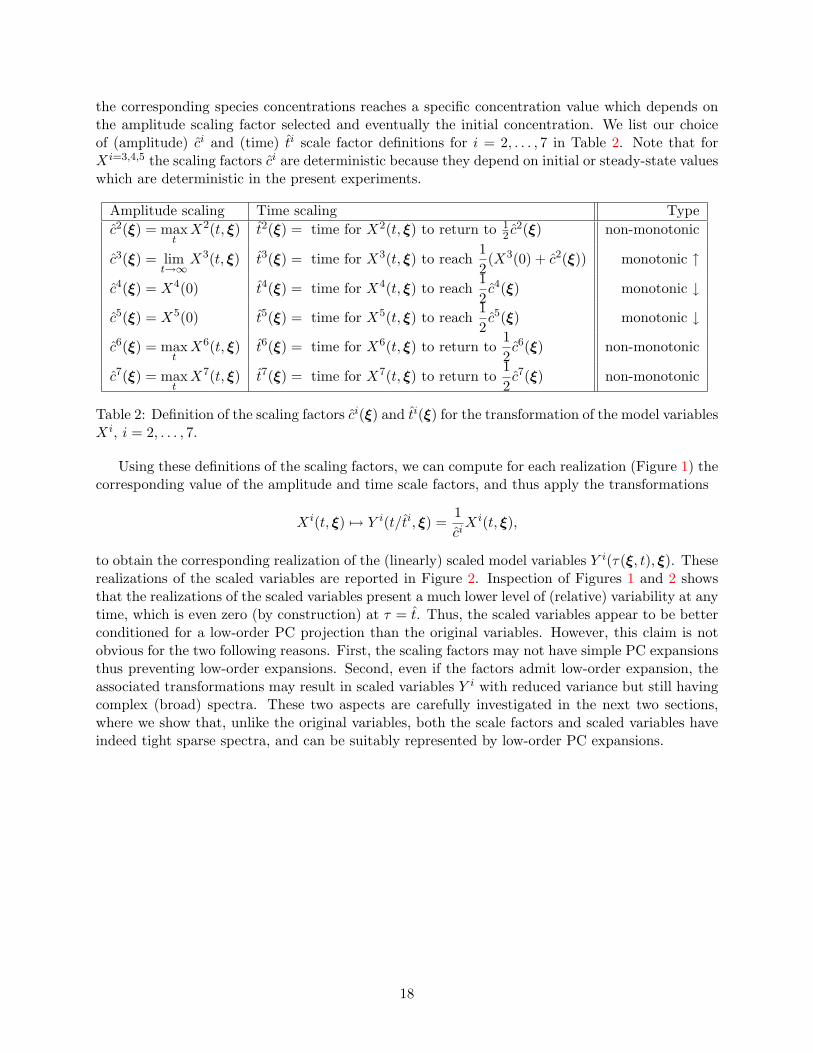
Using these definitions of the scaling factors, we can compute for each realization (Figure 1) thecorresponding value of the amplitude and time scale factors, and thus apply the transformations

Xi(t, ξ) 7→ Y i(t/ti, ξ) =1ciXi(t, ξ),

to obtain the corresponding realization of the (linearly) scaled model variables Y i(τ(ξ, t), ξ). Theserealizations of the scaled variables are reported in Figure 2. Inspection of Figures 1 and 2 showsthat the realizations of the scaled variables present a much lower level of (relative) variability at anytime, which is even zero (by construction) at τ = t. Thus, the scaled variables appear to be betterconditioned for a low-order PC projection than the original variables. However, this claim is notobvious for the two following reasons. First, the scaling factors may not have simple PC expansionsthus preventing low-order expansions. Second, even if the factors admit low-order expansion, theassociated transformations may result in scaled variables Y i with reduced variance but still havingcomplex (broad) spectra. These two aspects are carefully investigated in the next two sections,where we show that, unlike the original variables, both the scale factors and scaled variables haveindeed tight sparse spectra, and can be suitably represented by low-order PC expansions.

18

0 5 10 15 200

0.2

0.4

0.6

0.8

1[O2] (scaled)

τ

Y5 (τ

, ξ)

0 5 10 15 200.9995

0.9996

0.9997

0.9998

0.9999

1[H2O] (scaled)

τ

Y3 (τ

, ξ)

0 2 4 6 8 100

0.2

0.4

0.6

0.8

1[HO2] (scaled)

τ

Y6 (τ

, ξ)

0 1 2 3 4 50

0.2

0.4

0.6

0.8

1[H] (scaled)

τ

Y2 (τ

, ξ)

Figure 2: Scaled variables versus stretched time. Individual curves are obtained by transformingthe original realizations shown in Figure 1.

19

5 Application of the Preconditioned NISP

In this section, the preconditioning strategy is applied to the hydrogen oxidation problem. Wefocus our discussion on the species whose dynamics were discussed in the previous section. First,we carefully examine the scaling factors c and t and demonstrate that they are well behaved andadmit low order PC representations. Next, we show that the preconditioning effectively allows forlow order PC representations in the transformed space, while still capturing complex features ofthe original variables through the recovery procedure. In particular, we show that the precondi-tioned NISP allows for recovery of complicated (possibly bimodal) distributions via low order PCexpansions. We delay quantitative assessments of the method’s accuracy to Section 6.

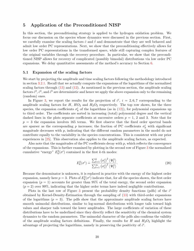
5.1 Expansion of the scaling factors

We start by projecting the amplitude and time scaling factors following the methodology introducedin section 3.2.1. Recall that we actually compute the expansions of the logarithms of the normalizedscaling factors through (13) and (12). As mentioned in the previous section, the amplitude scalingfactors c3, c4, and c5 are deterministic and hence we apply the above expansion only to the remaining(random) ones.

In Figure 3, we report the results for the projection of ci, i = 2, 6, 7 corresponding to theamplitude scaling factors for H, HO2 and H2O2 respectively. The top row shows, for the threespecies, the expansion coefficients σik of the logarithms (as in (12)), for polynomial expansions upto third order. The coefficients are sorted in increasing (total) polynomial degree and the verticaldashed lines in the plots separate coefficients at successive orders p = 1, 2 and 3. Note that forp = 3 the expansion involves 165 terms. We first observe that the fixed order spectral bandsare sparser as the corresponding p increases; the fraction of PC coefficients σik with significantmagnitude decreases with p, indicating that the different random parameters in the model do notcontribute equally to the variability in the species concentrations. This is consistent with our priorexperiences in [25]. This observation also applies to the amplitude scaling factors, as expected.

Also note that the magnitudes of the PC coefficients decay with p, which reflects the convergenceof the expansions. This is further examined by plotting in the second row of Figure 3 the normalizedcumulative “energy” E2

k(σi) contained in the first k-th modes:

E2k(σi) .=

∑kl=1

(σil)2 ⟨Ψ2

l

⟩∑∞l=1

(σil)2 ⟨Ψ2

l

⟩ . (20)

Because the denominator is unknown, it is replaced in practice with the energy of the highest orderexpansion, namely here p = 3. Plots of E2

k(σi) indicate that, for all the species shown, the first orderexpansion (p = 1) accounts for greater than 95% of the total energy, the second order expansion(p = 2) over 99%, indicating that the higher order terms have indeed negligible contributions.

Plots in the last row of Figure 3 present the probability density functions (pdfs) of the ci

obtained by Kernel-Density-Estimation through the sampling of (13) with third-order expansionsof the logarithms (p = 3). The pdfs show that the approximate amplitude scaling factors havesmooth unimodal distributions, similar to log-normal distributions with longer tails toward highvalues and sharper tails toward the lower amplitudes. The large coefficients of variation of thesedistributions have to be underlined since they directly reflect the sensitivity of the chemical systemdynamics to the random parameters. The unimodal character of the pdfs also confirms the validityof the amplitude scaling factors definitions. Finally, the results for H and H2O2 highlight theadvantage of projecting the logarithms, namely in preserving the positivity of ci.

20

0 50 100 150−0.6

−0.4

−0.2

0

0.2

0.4

0.6

p=1

p=2

H

0 50 100 150

−0.2

−0.1

0

0.1

0.2

p=1

p=2

HO2

0 50 100 150−0.6

−0.4

−0.2

0

0.2

0.4

0.6

p=1

p=2

H2O2

0 50 100 1500

0.2

0.4

0.6

0.8

1

1.2

p=1

p=2

0 50 100 1500

0.2

0.4

0.6

0.8

1

1.2

p=1

p=2

0 50 100 1500

0.2

0.4

0.6

0.8

1

1.2

p=1

p=2

−2 0 2 4x 10

−14

−5

0

5

10

15x 1013 H

0 0.5 1 1.5x 10

−9

−1

0

1

2

3x 109 HO2

−1 0 1 2 3x 10

−8

−5

0

5

10

15

20x 107 H2O2

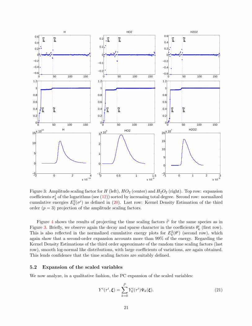
Figure 3: Amplitude scaling factor forH (left), HO2 (center) andH2O2 (right). Top row: expansioncoefficients σik of the logarithms (see (12)) sorted by increasing total degree. Second row: normalizedcumulative energies E2

k(σi) as defined in (20). Last row: Kernel Density Estimation of the thirdorder (p = 3) projection of the amplitude scaling factors.

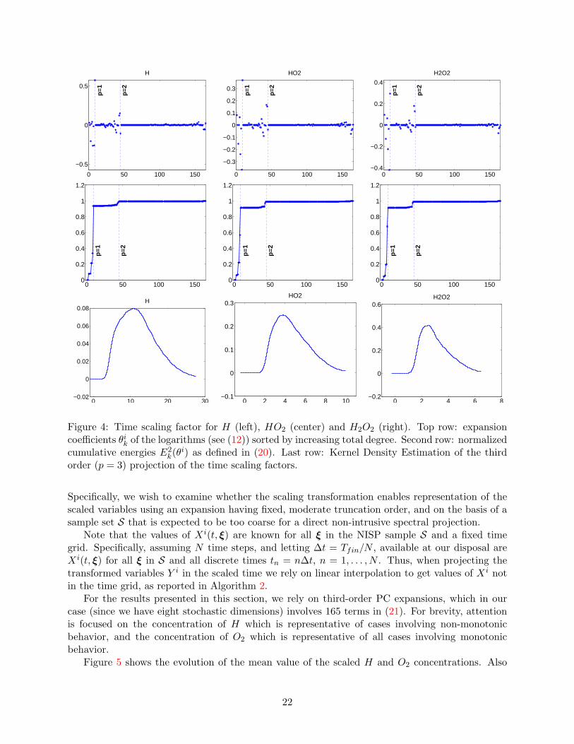
Figure 4 shows the results of projecting the time scaling factors ti for the same species as inFigure 3. Briefly, we observe again the decay and sparse character in the coefficients θik (first row).This is also reflected in the normalized cumulative energy plots for E2

k(θi) (second row), whichagain show that a second-order expansion accounts more than 99% of the energy. Regarding theKernel Density Estimations of the third order approximate of the random time scaling factors (lastrow), smooth log-normal like distributions, with large coefficients of variations, are again obtained.This lends confidence that the time scaling factors are suitably defined.

5.2 Expansion of the scaled variables

We now analyze, in a qualitative fashion, the PC expansion of the scaled variables:

Y i(τ i, ξ) =P∑k=0

Y ik (τ i)Ψk(ξ). (21)

21

0 50 100 150

−0.5

0

0.5

p=1

p=2

H

0 50 100 150

−0.3

−0.2

−0.1

0

0.1

0.2

0.3

p=1

p=2

HO2

0 50 100 150−0.4

−0.2

0

0.2

0.4

p=1

p=2

H2O2

0 50 100 1500

0.2

0.4

0.6

0.8

1

1.2

p=1

p=2

0 50 100 1500

0.2

0.4

0.6

0.8

1

1.2

p=1

p=2

0 50 100 1500

0.2

0.4

0.6

0.8

1

1.2

p=1

p=2

0 10 20 30−0.02

0

0.02

0.04

0.06

0.08H

0 2 4 6 8 10−0.1

0

0.1

0.2

0.3HO2

0 2 4 6 8−0.2

0

0.2

0.4

0.6H2O2

Figure 4: Time scaling factor for H (left), HO2 (center) and H2O2 (right). Top row: expansioncoefficients θik of the logarithms (see (12)) sorted by increasing total degree. Second row: normalizedcumulative energies E2

k(θi) as defined in (20). Last row: Kernel Density Estimation of the thirdorder (p = 3) projection of the time scaling factors.

Specifically, we wish to examine whether the scaling transformation enables representation of thescaled variables using an expansion having fixed, moderate truncation order, and on the basis of asample set S that is expected to be too coarse for a direct non-intrusive spectral projection.

Note that the values of Xi(t, ξ) are known for all ξ in the NISP sample S and a fixed timegrid. Specifically, assuming N time steps, and letting ∆t = Tfin/N , available at our disposal areXi(t, ξ) for all ξ in S and all discrete times tn = n∆t, n = 1, . . . , N . Thus, when projecting thetransformed variables Y i in the scaled time we rely on linear interpolation to get values of Xi notin the time grid, as reported in Algorithm 2.

For the results presented in this section, we rely on third-order PC expansions, which in ourcase (since we have eight stochastic dimensions) involves 165 terms in (21). For brevity, attentionis focused on the concentration of H which is representative of cases involving non-monotonicbehavior, and the concentration of O2 which is representative of all cases involving monotonicbehavior.

Figure 5 shows the evolution of the mean value of the scaled H and O2 concentrations. Also

22

plotted are dashed lines indicating the range of ±2σ bounds, where σ is the local standard deviation.The latter is evaluated from the coefficients of the truncated PC expansion (21), according to:

σi(τ i) =

(P∑k=1

[Y ik (τi)

]2 〈Ψk〉2)1/2

Comparing the results in Figure 5 to the corresponding realization plotted in Figure 2, suggeststhat, though of moderate order, the PC expansion of the scaled variables is able to capture broadfeatures of their evolution. In particular, the variance of the scaled solution, estimated from thePC expansion and visualized using dashed lines, appears to collapse at the stretched time τ = 1.

0 1 2 3 4−0.4

−0.2

0

0.2

0.4

0.6

0.8

1

1.2

1.4[H]

τ0 2 4 6 8

0

0.2

0.4

0.6

0.8

1

1.2

1.4[O2]

τ

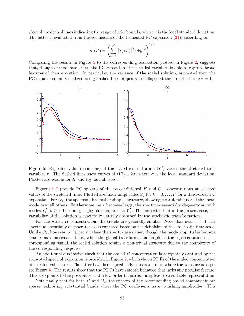
Figure 5: Expected value (solid line) of the scaled concentration 〈Y i〉 versus the stretched timevariable, τ . The dashed lines show curves of 〈Y i〉 ± 2σ, where σ is the local standard deviation.Plotted are results for H and O2, as indicated.

Figures 6–7 provide PC spectra of the preconditioned H and O2 concentrations at selectedvalues of the stretched time. Plotted are mode amplitudes Y i

k for k = 0, . . . , P for a third-order PCexpansion. For O2, the spectrum has rather simple structure, showing clear dominance of the meanmode over all others. Furthermore, as τ becomes large, the spectrum essentially degenerates, withmodes Y 5

k , k ≥ 1, becoming negligible compared to Y 50 . This indicates that in the present case, the

variability of the solution is essentially entirely absorbed by the stochastic transformation.For the scaled H concentration, the trends are generally similar. Note that near τ = 1, the

spectrum essentially degenerates, as is expected based on the definition of the stochastic time scale.Unlike O2, however, at larger τ values the spectra are richer, though the mode amplitudes becomesmaller as τ increases. Thus, while the global transformation simplifies the representation of thecorresponding signal, the scaled solution retains a non-trivial structure due to the complexity ofthe corresponding response.

An additional qualitative check that the scaled H concentration is adequately captured by thetruncated spectral expansion is provided in Figure 8, which shows PDFs of the scaled concentrationat selected values of τ . The latter have been specifically chosen at times where the variance is large,see Figure 5. The results show that the PDFs have smooth behavior that lacks any peculiar feature.This also points to the possibility that a low order truncation may lead to a suitable representation.

Note finally that for both H and O2, the spectra of the corresponding scaled components aresparse, exhibiting substantial bands where the PC coefficients have vanishing amplitudes. This

23

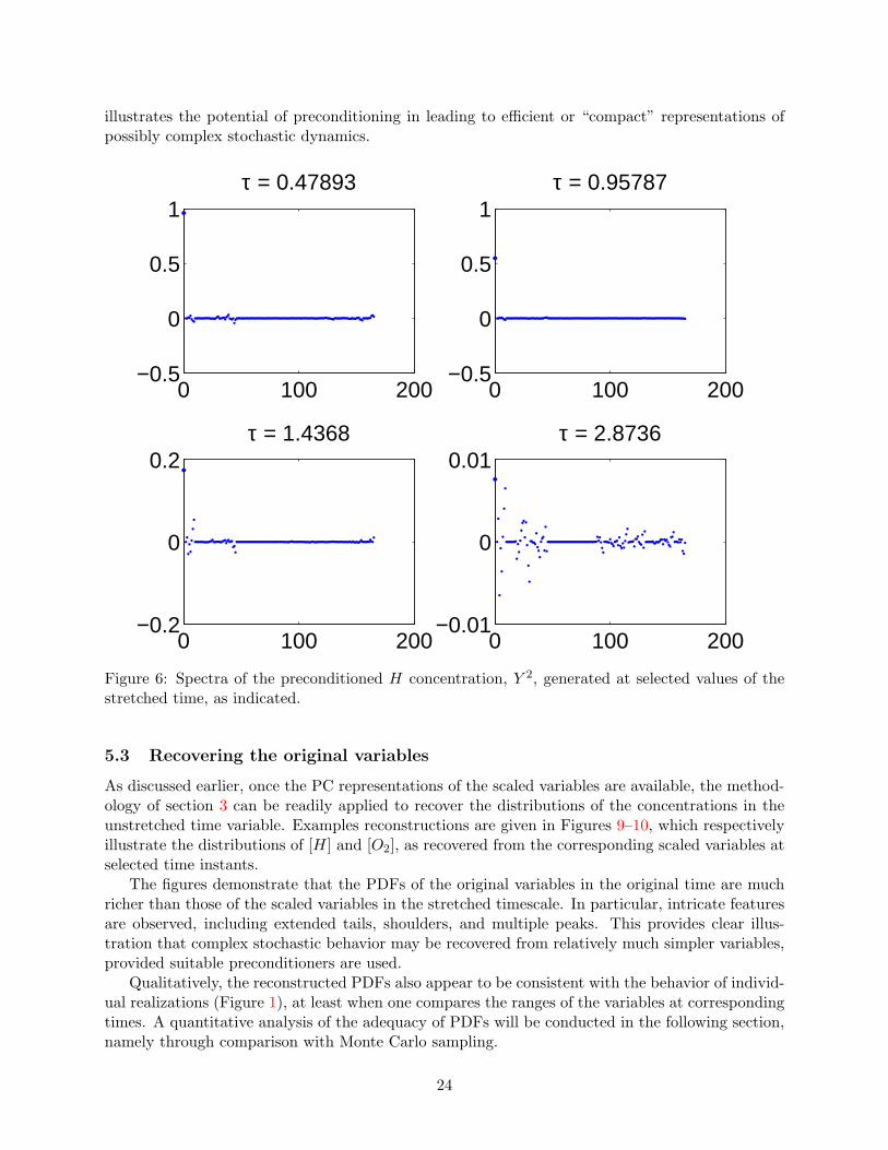
illustrates the potential of preconditioning in leading to efficient or “compact” representations ofpossibly complex stochastic dynamics.

0 100 200−0.5

0

0.5

1τ = 0.47893

0 100 200−0.5

0

0.5

1τ = 0.95787

0 100 200−0.2

0

0.2τ = 1.4368

0 100 200−0.01

0

0.01τ = 2.8736

Figure 6: Spectra of the preconditioned H concentration, Y 2, generated at selected values of thestretched time, as indicated.

5.3 Recovering the original variables

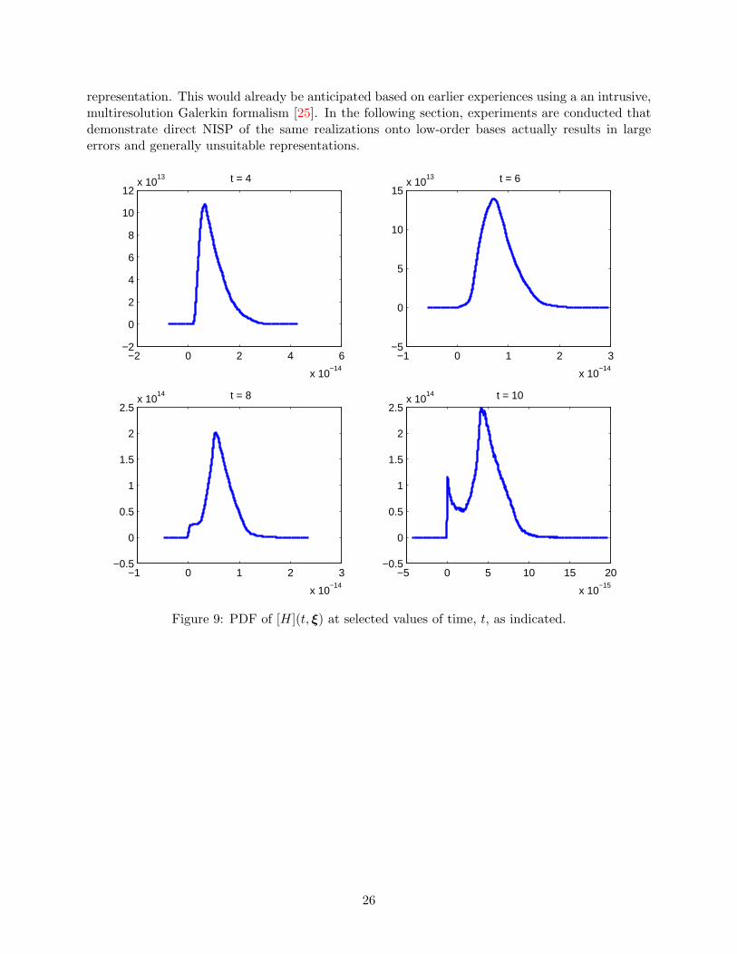
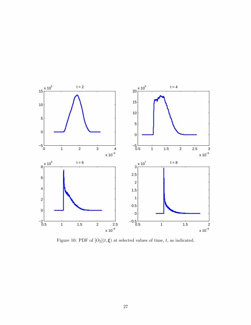
As discussed earlier, once the PC representations of the scaled variables are available, the method-ology of section 3 can be readily applied to recover the distributions of the concentrations in theunstretched time variable. Examples reconstructions are given in Figures 9–10, which respectivelyillustrate the distributions of [H] and [O2], as recovered from the corresponding scaled variables atselected time instants.

The figures demonstrate that the PDFs of the original variables in the original time are muchricher than those of the scaled variables in the stretched timescale. In particular, intricate featuresare observed, including extended tails, shoulders, and multiple peaks. This provides clear illus-tration that complex stochastic behavior may be recovered from relatively much simpler variables,provided suitable preconditioners are used.

Qualitatively, the reconstructed PDFs also appear to be consistent with the behavior of individ-ual realizations (Figure 1), at least when one compares the ranges of the variables at correspondingtimes. A quantitative analysis of the adequacy of PDFs will be conducted in the following section,namely through comparison with Monte Carlo sampling.

24

0 100 200−0.2

0

0.2τ = 2.5953

0 100 200−0.02

0

0.02

0.04τ = 5.1907

0 100 200−0.01

0

0.01

0.02τ = 7.786

0 100 200−5

0

5

10x 10

−3 τ = 15.572

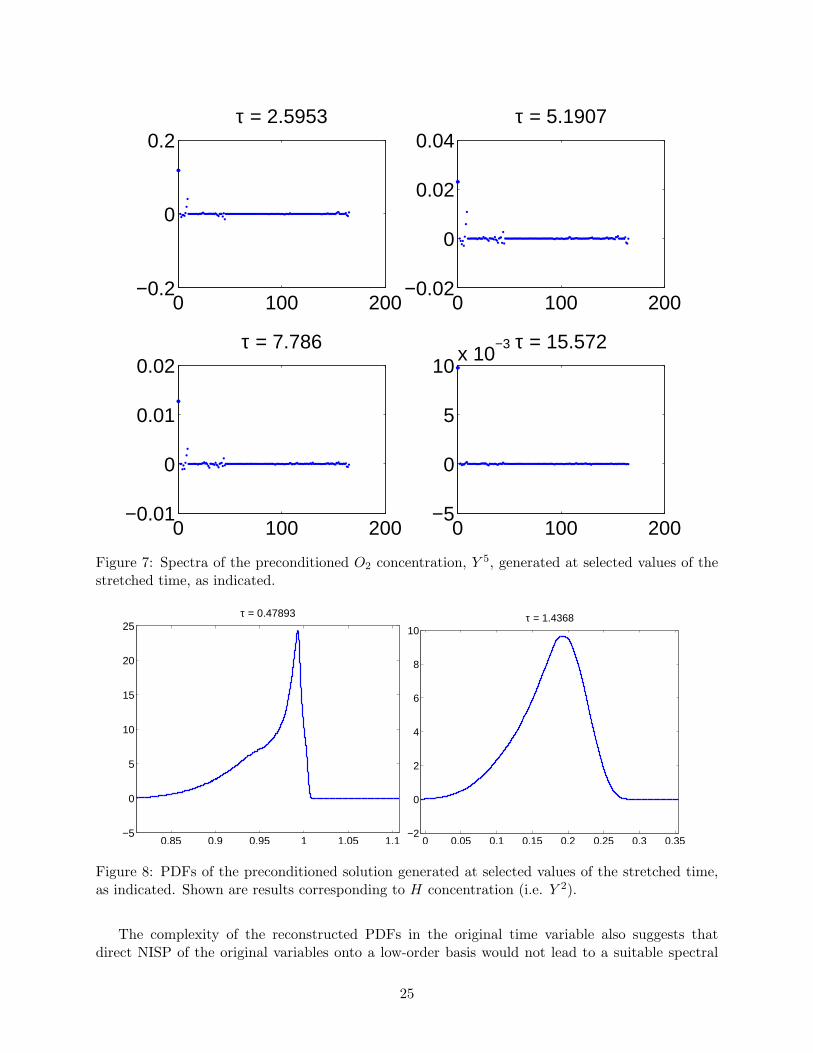
Figure 7: Spectra of the preconditioned O2 concentration, Y 5, generated at selected values of thestretched time, as indicated.

0.85 0.9 0.95 1 1.05 1.1−5

0

5

10

15

20

25τ = 0.47893

0 0.05 0.1 0.15 0.2 0.25 0.3 0.35−2

0

2

4

6

8

10τ = 1.4368

Figure 8: PDFs of the preconditioned solution generated at selected values of the stretched time,as indicated. Shown are results corresponding to H concentration (i.e. Y 2).

The complexity of the reconstructed PDFs in the original time variable also suggests thatdirect NISP of the original variables onto a low-order basis would not lead to a suitable spectral

25

representation. This would already be anticipated based on earlier experiences using a an intrusive,multiresolution Galerkin formalism [25]. In the following section, experiments are conducted thatdemonstrate direct NISP of the same realizations onto low-order bases actually results in largeerrors and generally unsuitable representations.

−2 0 2 4 6

x 10−14

−2

0

2

4

6

8

10

12x 10

13 t = 4

−1 0 1 2 3

x 10−14

−5

0

5

10

15x 10

13 t = 6

−1 0 1 2 3

x 10−14

−0.5

0

0.5

1

1.5

2

2.5x 10

14 t = 8

−5 0 5 10 15 20

x 10−15

−0.5

0

0.5

1

1.5

2

2.5x 10

14 t = 10

Figure 9: PDF of [H](t, ξ) at selected values of time, t, as indicated.

26

0 1 2 3 4

x 10−6

−5

0

5

10

15x 10

5 t = 2

0.5 1 1.5 2 2.5 3

x 10−6

−5

0

5

10

15

20x 10

5 t = 4

0.5 1 1.5 2 2.5

x 10−6

−2

0

2

4

6

8x 10

6 t = 6

0.5 1 1.5 2

x 10−6

−0.5

0

0.5

1

1.5

2

2.5

3x 10

7 t = 8

Figure 10: PDF of [O2](t, ξ) at selected values of time, t, as indicated.

27

6 Convergence study

In this section, we assess the advantages achieved by preconditioning, particularly by contrastingthe performance of preconditioned and conventional NISP.

6.1 Error estimates

We denote ‖·‖L2(Ω∗)

the L2-norm in the image space (Ω∗,B(Ω∗), Fξ) (see section 2):

‖X(t, ·)‖L2(Ω∗)

= (X(t, ·), X(t, ·))1/2 .

For t ≥ 0, we define the normalized approximation error on X(t, ·), denoted by ε(t), according to:

ε(t) =

∥∥∥X(t, ·)− X(t, ·)∥∥∥

L2(Ω∗)

‖X(t, ·)‖L2(Ω∗)

, (22)

where, following the notations of section 3.3, X is the recovered variable that approximates X.Obviously, since the exact solution X(t, ·) is not known we shall instead rely on Monte Carlosamples to estimate ε. Specifically, denoting S a sample set of ξ ∈ Ω∗ drawn from the distributionFξ, and letting |S| denote the size of the sample set S, we shall make use of

ε(t) = lim|S|→∞

∑ξ∈S

(X(t, ξ)− X(t, ξ))2

∑ξ∈S

(X(t, ξ))2

1/2

, (23)

to estimate ε(t) from finite sample sets S. This error measurement will serve to quantify theapproximation errors associated to the different types of preconditioning strategies (linear / log-linear projection, Option 1 / Option 2 in Algorithm 2). Also of interest will be the convergence ofε(t) as the expansion order p increases, and comparison of the errors with the case of NISP withoutpreconditioning, that is when c = t = 1. In addition, because all species with index i = 2, . . . , 7exhibit similar error dependencies with regard to the expansion order, we only report measurementsfor the case of Xi=2 = [H], which has the most complex behavior. Also, for convenience, we dropthe superscript 2 from X2 and its transform Y 2 and simply refer to them as X and Y throughoutthis section.

6.2 Error analysis

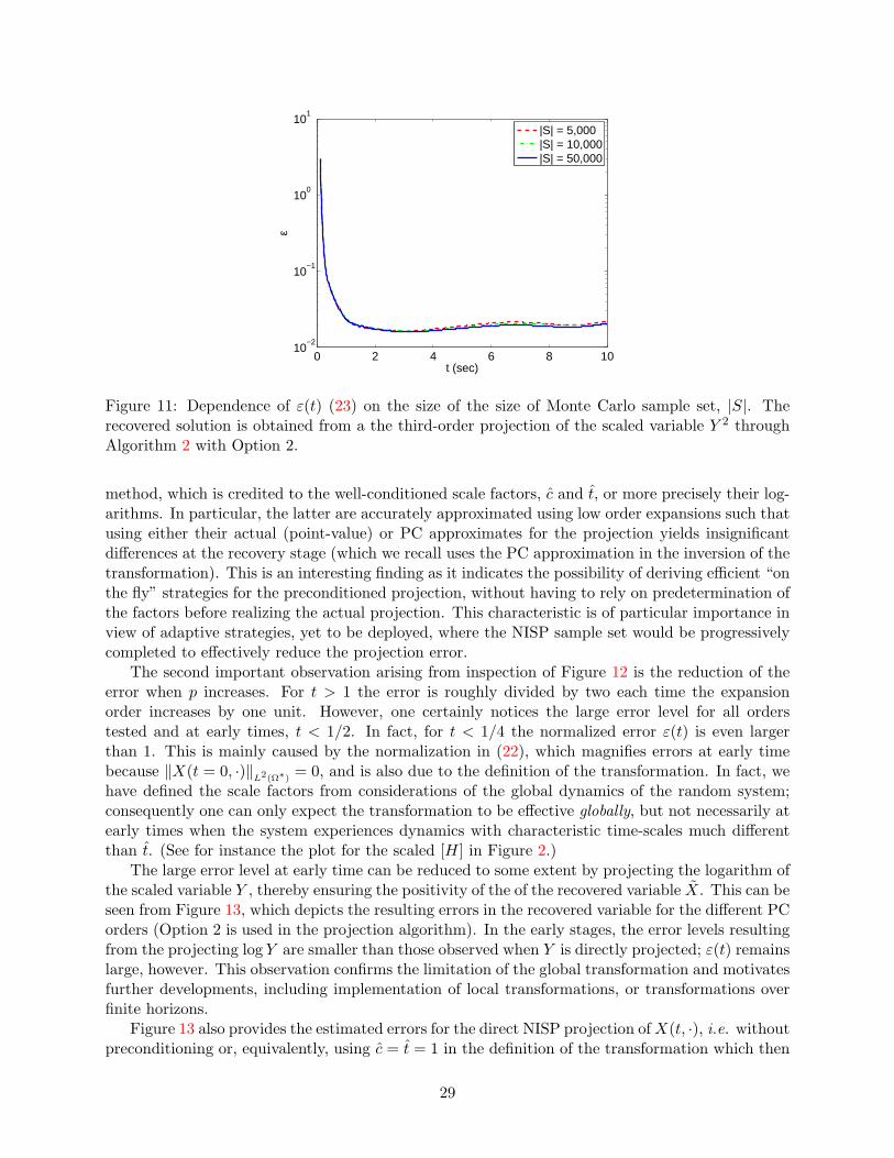
In a first series of tests, we monitor the convergence of the error estimate (23) for increasingly largeMonte-Carlo sample set. A typical illustration of the convergence of ε(t) as |S| increases is reportedin Figure 11. The plot shows that ε is fairly well estimated using a sample set with |S| = 50, 000,a value that is used in all subsequent computations.

Next, we compare in Figure 12 the errors in the recovered concentration of H at differentunscaled times. The left plot corresponds to the case of the recovery from the preconditioned pro-jections Algorithm 2 using Option-1 for the definition of the factors in the transformation, while theright plot corresponds to Option 2. In both cases, results are shown for truncated PC expansionswith order p = 1, 2, and 3. We first remark that the two options used in the projection algo-rithm yield comparable error levels. This demonstrates the robustness of the proposed projection

28

0 2 4 6 8 1010

−2

10−1

100

101

t (sec)

ε

|S| = 5,000|S| = 10,000|S| = 50,000

Figure 11: Dependence of ε(t) (23) on the size of the size of Monte Carlo sample set, |S|. Therecovered solution is obtained from a the third-order projection of the scaled variable Y 2 throughAlgorithm 2 with Option 2.

method, which is credited to the well-conditioned scale factors, c and t, or more precisely their log-arithms. In particular, the latter are accurately approximated using low order expansions such thatusing either their actual (point-value) or PC approximates for the projection yields insignificantdifferences at the recovery stage (which we recall uses the PC approximation in the inversion of thetransformation). This is an interesting finding as it indicates the possibility of deriving efficient “onthe fly” strategies for the preconditioned projection, without having to rely on predetermination ofthe factors before realizing the actual projection. This characteristic is of particular importance inview of adaptive strategies, yet to be deployed, where the NISP sample set would be progressivelycompleted to effectively reduce the projection error.

The second important observation arising from inspection of Figure 12 is the reduction of theerror when p increases. For t > 1 the error is roughly divided by two each time the expansionorder increases by one unit. However, one certainly notices the large error level for all orderstested and at early times, t < 1/2. In fact, for t < 1/4 the normalized error ε(t) is even largerthan 1. This is mainly caused by the normalization in (22), which magnifies errors at early timebecause ‖X(t = 0, ·)‖

L2(Ω∗)= 0, and is also due to the definition of the transformation. In fact, we

have defined the scale factors from considerations of the global dynamics of the random system;consequently one can only expect the transformation to be effective globally, but not necessarily atearly times when the system experiences dynamics with characteristic time-scales much differentthan t. (See for instance the plot for the scaled [H] in Figure 2.)

The large error level at early time can be reduced to some extent by projecting the logarithm ofthe scaled variable Y , thereby ensuring the positivity of the of the recovered variable X. This can beseen from Figure 13, which depicts the resulting errors in the recovered variable for the different PCorders (Option 2 is used in the projection algorithm). In the early stages, the error levels resultingfrom the projecting log Y are smaller than those observed when Y is directly projected; ε(t) remainslarge, however. This observation confirms the limitation of the global transformation and motivatesfurther developments, including implementation of local transformations, or transformations overfinite horizons.

Figure 13 also provides the estimated errors for the direct NISP projection ofX(t, ·), i.e. withoutpreconditioning or, equivalently, using c = t = 1 in the definition of the transformation which then

29

Option 1 Option 2

0 2 4 6 8 1010

−2

10−1

100

101

102

t (sec)

ε

p = 1p = 2p = 3

0 2 4 6 8 1010

−2

10−1

100

101

102

t (sec)

ε

p = 1p = 2p = 3

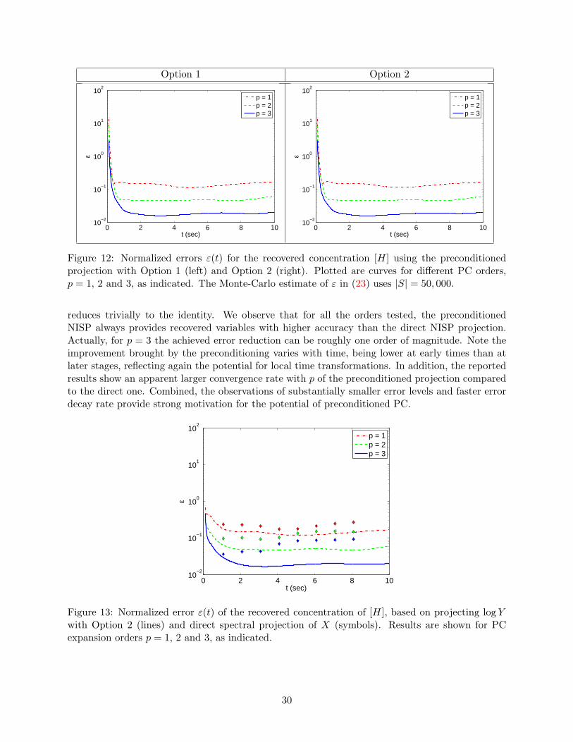
Figure 12: Normalized errors ε(t) for the recovered concentration [H] using the preconditionedprojection with Option 1 (left) and Option 2 (right). Plotted are curves for different PC orders,p = 1, 2 and 3, as indicated. The Monte-Carlo estimate of ε in (23) uses |S| = 50, 000.

reduces trivially to the identity. We observe that for all the orders tested, the preconditionedNISP always provides recovered variables with higher accuracy than the direct NISP projection.Actually, for p = 3 the achieved error reduction can be roughly one order of magnitude. Note theimprovement brought by the preconditioning varies with time, being lower at early times than atlater stages, reflecting again the potential for local time transformations. In addition, the reportedresults show an apparent larger convergence rate with p of the preconditioned projection comparedto the direct one. Combined, the observations of substantially smaller error levels and faster errordecay rate provide strong motivation for the potential of preconditioned PC.

0 2 4 6 8 1010

−2

10−1

100

101

102

t (sec)

ε

p = 1p = 2p = 3

Figure 13: Normalized error ε(t) of the recovered concentration of [H], based on projecting log Ywith Option 2 (lines) and direct spectral projection of X (symbols). Results are shown for PCexpansion orders p = 1, 2 and 3, as indicated.

30

6.3 Convergence in distribution

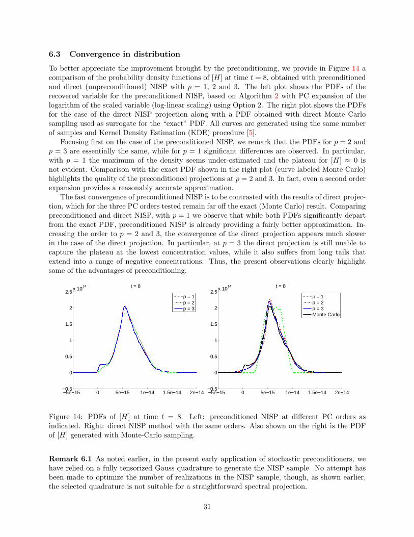
To better appreciate the improvement brought by the preconditioning, we provide in Figure 14 acomparison of the probability density functions of [H] at time t = 8, obtained with preconditionedand direct (unpreconditioned) NISP with p = 1, 2 and 3. The left plot shows the PDFs of therecovered variable for the preconditioned NISP, based on Algorithm 2 with PC expansion of thelogarithm of the scaled variable (log-linear scaling) using Option 2. The right plot shows the PDFsfor the case of the direct NISP projection along with a PDF obtained with direct Monte Carlosampling used as surrogate for the “exact” PDF. All curves are generated using the same numberof samples and Kernel Density Estimation (KDE) procedure [5].

Focusing first on the case of the preconditioned NISP, we remark that the PDFs for p = 2 andp = 3 are essentially the same, while for p = 1 significant differences are observed. In particular,with p = 1 the maximum of the density seems under-estimated and the plateau for [H] ≈ 0 isnot evident. Comparison with the exact PDF shown in the right plot (curve labeled Monte Carlo)highlights the quality of the preconditioned projections at p = 2 and 3. In fact, even a second orderexpansion provides a reasonably accurate approximation.

The fast convergence of preconditioned NISP is to be contrasted with the results of direct projec-tion, which for the three PC orders tested remain far off the exact (Monte Carlo) result. Comparingpreconditioned and direct NISP, with p = 1 we observe that while both PDFs significantly departfrom the exact PDF, preconditioned NISP is already providing a fairly better approximation. In-creasing the order to p = 2 and 3, the convergence of the direct projection appears much slowerin the case of the direct projection. In particular, at p = 3 the direct projection is still unable tocapture the plateau at the lowest concentration values, while it also suffers from long tails thatextend into a range of negative concentrations. Thus, the present observations clearly highlightsome of the advantages of preconditioning.

−5e−15 0 5e−15 1e−14 1.5e−14 2e−14−0.5

0

0.5

1

1.5

2

2.5x 10

14 t = 8

p = 1p = 2p = 3

−5e−15 0 5e−15 1e−14 1.5e−14 2e−14−0.5

0

0.5

1

1.5

2

2.5x 10

14 t = 8

p = 1p = 2p = 3Monte Carlo

Figure 14: PDFs of [H] at time t = 8. Left: preconditioned NISP at different PC orders asindicated. Right: direct NISP method with the same orders. Also shown on the right is the PDFof [H] generated with Monte-Carlo sampling.

Remark 6.1 As noted earlier, in the present early application of stochastic preconditioners, wehave relied on a fully tensorized Gauss quadrature to generate the NISP sample. No attempt hasbeen made to optimize the number of realizations in the NISP sample, though, as shown earlier,the selected quadrature is not suitable for a straightforward spectral projection.

31

It is interesting to note that with a Monte-Carlo approach, a sample size of 50, 000 was foundsufficient to approximate the PDF of the solution. This is significantly smaller than the NISP samplethat includes 58 = 390, 625 realizations. This may be misleading since it may suggest that thestochastic preconditioning approach is less efficient than MC. We should point out, however, that inpractice sparse quadratures are frequently used, which can dramatically reduce the number of NISPsamples. This would be feasible in the present case, because the stochastic preconditioning approachenables the use of low-order expansions. By means of example, using SMOLPACK [34] with a level6 sparse quadrature on the current eight-dimensional problem would lead to a NISP sample havingon the order of 6, 000 realizations. This would clearly support the low-order expansions affordedby stochastic preconditioning, with a number of realizations about one order of magnitude smallerthan with MC, and nearly two orders of magnitude smaller than the present fully tensorized Gaussquadrature.

32

7 Generalized preconditioners

So far we have demonstrated that preconditioning of realizations prior to projection potentiallyallows for a significant reduction in order of the PC representation and thus of computational efforts.This was demonstrated for 6 of the 7 species present in the hydrogen oxidation problem, for whichsimple scaling transformations were applied. It is clear that the complexity reduction achieved bythe preconditioned projection depends on the appropriateness of the underlying transformations.In particular, we have seen that the transformation has to incorporate two essential features: itshould ensure a) the proper definition of the scaling factors for all realizations and b) yield PCrepresentation with rapid spectral decay at all times of interest for the transformed variable. It isthen legitimate to ask whether any dynamical system possesses a transformation satisfying thosetwo requirements. Clearly, as far as simple scaling transformations are considered, the answer isnegative and the case of OH, discussed below, is an example of such breakdown. This fact doesnot, however, imply that the preconditioning has limited scope, but merely that one should becareful when choosing the transformations on which the preconditioning would be based. In thefollowing, we illustrate these issues in light of the behavior for the stochastic OH concentration.

7.1 Random dynamics of OH

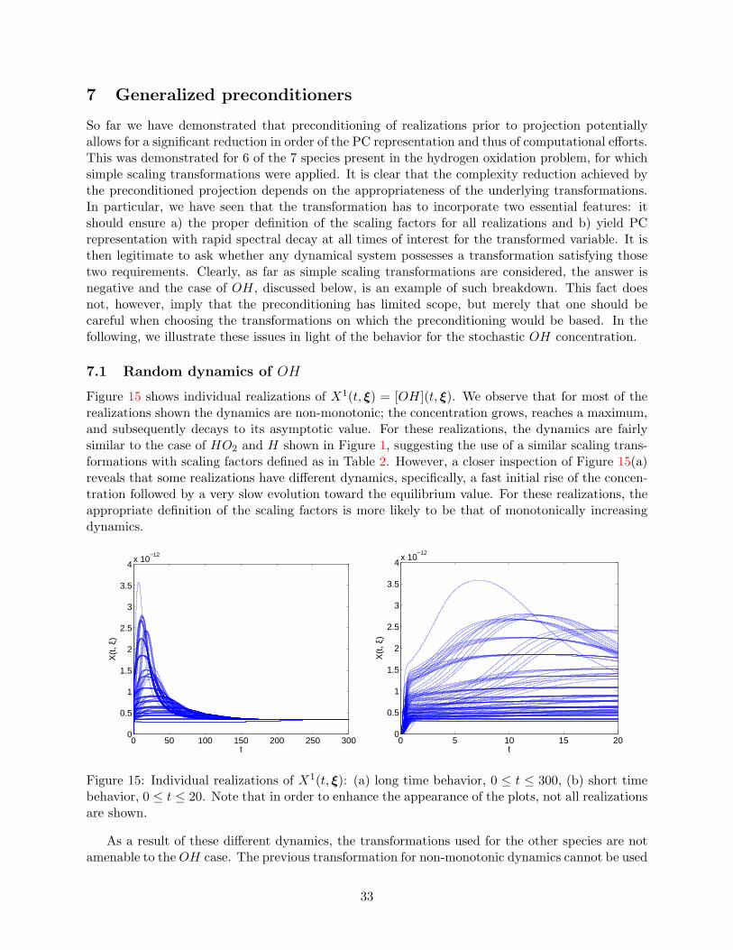
Figure 15 shows individual realizations of X1(t, ξ) = [OH](t, ξ). We observe that for most of therealizations shown the dynamics are non-monotonic; the concentration grows, reaches a maximum,and subsequently decays to its asymptotic value. For these realizations, the dynamics are fairlysimilar to the case of HO2 and H shown in Figure 1, suggesting the use of a similar scaling trans-formations with scaling factors defined as in Table 2. However, a closer inspection of Figure 15(a)reveals that some realizations have different dynamics, specifically, a fast initial rise of the concen-tration followed by a very slow evolution toward the equilibrium value. For these realizations, theappropriate definition of the scaling factors is more likely to be that of monotonically increasingdynamics.

0 50 100 150 200 250 3000

0.5

1

1.5

2

2.5

3

3.5

4x 10

−12

t

X(t

, ξ)

0 5 10 15 200

0.5

1

1.5

2

2.5

3

3.5

4x 10

−12

t

X(t

, ξ)

Figure 15: Individual realizations of X1(t, ξ): (a) long time behavior, 0 ≤ t ≤ 300, (b) short timebehavior, 0 ≤ t ≤ 20. Note that in order to enhance the appearance of the plots, not all realizationsare shown.

As a result of these different dynamics, the transformations used for the other species are notamenable to the OH case. The previous transformation for non-monotonic dynamics cannot be used

33

as some realizations do not exhibit an intermediate maximum. On the other hand, the transformdesigned previously for monotonically increasing concentration is not suited to non-monotonicrealizations and yields an ineffective preconditioning.

One can think of two alternatives to address this issue. First, one could use different transfor-mation types, depending on ξ; this corresponds to the general idea of local approximation basedon the partitioning of Ω∗, as used for instance in adaptive intrusive methods. This idea, althoughattractive, will not be pursued here because of the need for efficient strategies to construct thepartition of the random parameter domain. Alternatively, one can think of more general transfor-mations having almost surely well defined scaling factors and yielding transformed variables withtight PC spectra. Being more aligned with the preconditioning of the other species, this latteralternative is followed below.

Since this section is only concerned with X1 = [OH], we drop in the following the superscriptin X1 and Y 1, and simply use X and Y .

7.2 Stochastic transformation for OH

The objective is to define a transformation such that the random dynamics remain essentiallysimilar (in phase) for almost every ξ ∈ Ω∗. We address this issue by considering an affine scalingtransformation as follows. We begin by defining a deterministic reference dynamics, Xref through

Xref (t) = X∞(1− exp(−λt)

), λ = 1/100,

with X∞ the deterministic steady state OH concentration (uniquely determined by determinis-tic equilibrium constants and deterministic initial concentrations). This reference ensures thatX(t, ξ) − Xref (t) has almost surely a non-monotonic dynamics consisting in an increasing stage,followed by a decaying stage: X(t, ξ) −Xref (t) present almost surely a local maximum. This, inturn, ensures well-defined scaling factors c and t as

c(ξ) = maxt

(X(t, ξ)−Xref (t)

),

t(ξ) = time taken for(X(t, ξ)−Xref (t)

)to return to 1

2 c(ξ).

With these scaling factors, we define the transformation Φ according to

Φ[X(t, ξ); c

]=

1c(ξ)

(X(t, ξ)−Xref (t)

), (24)

and consider the scaled variable Y(τ(t, ξ), ξ

)= Φ

[X(t, ξ)

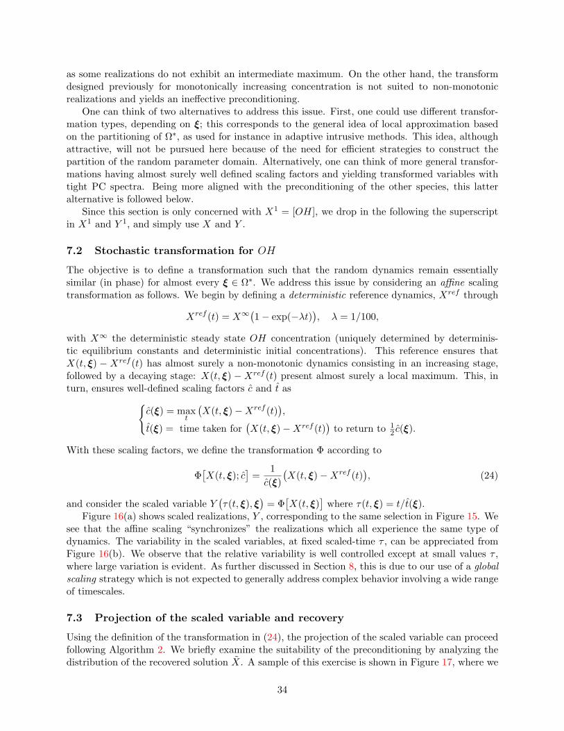
]where τ(t, ξ) = t/t(ξ).

Figure 16(a) shows scaled realizations, Y , corresponding to the same selection in Figure 15. Wesee that the affine scaling “synchronizes” the realizations which all experience the same type ofdynamics. The variability in the scaled variables, at fixed scaled-time τ , can be appreciated fromFigure 16(b). We observe that the relative variability is well controlled except at small values τ ,where large variation is evident. As further discussed in Section 8, this is due to our use of a globalscaling strategy which is not expected to generally address complex behavior involving a wide rangeof timescales.

7.3 Projection of the scaled variable and recovery

Using the definition of the transformation in (24), the projection of the scaled variable can proceedfollowing Algorithm 2. We briefly examine the suitability of the preconditioning by analyzing thedistribution of the recovered solution X. A sample of this exercise is shown in Figure 17, where we

34

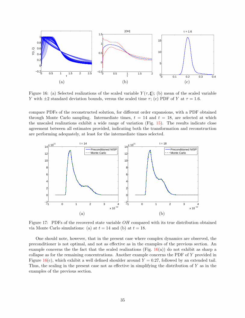
0 0.5 1 1.5 2 2.5−0.2

0

0.2

0.4

0.6

0.8

1

τ

Y(τ

, ξ)

0 0.5 1 1.5 2−0.5

0

0.5

1

1.5[OH]

τ 0 0.1 0.2 0.3 0.40

5

10

15

τ = 1.6

(a) (b) (c)

Figure 16: (a) Selected realizations of the scaled variable Y (τ, ξ); (b) mean of the scaled variableY with ±2 standard deviation bounds, versus the scaled time τ ; (c) PDF of Y at τ = 1.6.

compare PDFs of the reconstructed solution, for different order expansions, with a PDF obtainedthrough Monte Carlo sampling. Intermediate times, t = 14 and t = 18, are selected at whichthe unscaled realizations exhibit a wide range of variation (Fig. 15). The results indicate closeagreement between all estimates provided, indicating both the transformation and reconstructionare performing adequately, at least for the intermediate times selected.

−1 0 1 2 3 4

x 10−12

−2

0

2

4

6

8

10

12

14x 10

11 t = 14

Preconditioned NISPMonte Carlo

−1 0 1 2 3 4

x 10−12

−2

0

2

4

6

8

10

12

14x 10

11 t = 18

Preconditioned NISPMonte Carlo

(a) (b)

Figure 17: PDFs of the recovered state variable OH compared with its true distribution obtainedvia Monte Carlo simulations: (a) at t = 14 and (b) at t = 18.

One should note, however, that in the present case where complex dynamics are observed, thepreconditioner is not optimal, and not as effective as in the examples of the previous section. Anexample concerns the the fact that the scaled realizations (Fig. 16(a)) do not exhibit as sharp acollapse as for the remaining concentrations. Another example concerns the PDF of Y provided inFigure 16(c), which exhibit a well defined shoulder around Y = 0.27, followed by an extended tail.Thus, the scaling in the present case not as effective in simplifying the distribution of Y as in theexamples of the previous section.

35

8 Summary and discussion

This paper has focused on exploring the potential of a non-intrusive stochastic preconditioningformalism to enable efficient low-order PC representation of a complex stochastic dynamical system.The approach is illustrated for the case of a stiff oxidation problem with large uncertainties in rateparameters. The system had been known to exhibit a complex dependence on the stochastic rateparameters leading to large variations in the response of individual species and in the correspondingresponse timescales.

A simplified, multiscale, preconditioning approach was considered that is based on judiciouslyexploiting a coarse computational database of individual realizations. The database is used to defineappropriate characteristic time and concentration scales for each species and each of the realizations.A NISP approach is then used to express these global characteristic scales in terms of appropriate,low-order PC expansions, and the latter are used to scale individual realizations. NISP is also usedto project the resulting stretched realizations onto the PC basis. This leads to a reprensentation ofthe response of the stochastic system in terms of an appropriate combination of the PC expansionsfor the preconditioners and for the stretched variables. Computational experiments conducted usinga coarse computed database showed that the preconditioning approach can lead to low-order PCrepresentations with rapid spectral decay, and that the latter may be efficiently sampled to recoverthe distribution of the original variables in the physical timescale.

Despite their limited scope, the present experiences naturally lead to a number of basic obser-vations, and motivate further extensions. We conclude this paper with listing a few of these:

1. The computations and analyses discussed above relied heavily on the availability of a com-puted database of model realizations, which in particular enabled consideration of differentscalings and projection approaches, and systematic study of their associated properties. Forthe present problem, construction of the realization database was relatively straightforward,requiring moderate amount of storage and a small CPU overhead. Extension of the presentnon-intrusive methodology to larger-scale would naturally benefit from the availability oflarge databases, and of efficient schemes for storing, indexing, retrieving, interpolating andotherwise transforming individual realization data.

2. The implementations above relied on simple, linear or affine, scaling transformations in orderto (approximately) synchronize between different realizations and consequently define scaledvariables having variances that are significantly smaller than those of the unscaled variables.Once these transformations were selected, the database could be exploited in an automaticfashion in order to determine the stretching parameters suitable for each realization, andconsequently conduct the associated NISP. In more general settings, it may be worthwhileto consider larger families of transformations, and to determine “optimal” sets of stretchingparameters. Thus, it may be natural to approach the scaling of realizations as an optimizationproblem, constrained possibly by the requirement that the PC representation of the optimaltransformation be an invertible stochastic quantity. This would in particular ensure thatthe original variables can be recovered in the physical time domain. By building librariesof suitable transformations, such optimization approaches would offer the promise of a fullyautomated process for determining optimal preconditioners.

3. In the present implementations, a simplified approach was adopted for the purpose of rep-resenting the stochastic preconditioners and the preconditioned solution, i.e. the scaled vari-ables. Specifically, for both quantities, PC expansions were used that have the same trun-cation order. This is evidently not an essential requirement of the present methodology, as

36

expansions of different truncation order may be readily used for the preconditioner and forthe preconditioned solution. Though not considered in the present work, such mixed orderapproaches may provide additional means of controlling the properties of the overall repre-sentation, particularly to ensure that the latter can be well represented on the underlyinggrid of stochastic realizations. Another possibility that has not been considered here, andthat may be worthwhile to explore, concerns the use of mixed basis representations for thepreconditioner and the preconditioned solution. Depending on the nature of the precondi-tioner, such mixed representations may appear akin to enriched basis concepts that have beenrecently advanced for PC representations [13]. Specifically, a formal link between stochasticpreconditioning and enriched basis representations may be made evident if, instead of theusual, additive, enriched basis construction, one relies on a factorized construction in whichthe enriching functions appears as factors of a PC expansion. The resulting representationswould evidently share many similarities with the preconditioning constructs, though theywould not automatically incorporate multiscale time stretching.

4. A simplified approach to preconditioning the stochastic solution was adopted that was basedon the introduction of global time scales for individual components of the solution. While thissimplified approach appeared to be suitable for the examples treated, it should be emphasizedthat the resulting representation may not be necessarily optimal at all times. For instance,in both early stages of the ignition process and at very large time, a highly efficient localdescription of the stochastic solution may evidently be sought in terms of the Jacobian ofthe stochastic solution. Consequently, it may appear advantageous to seek extensions ofthe present formalism, in which preconditioned representations are localized over finite timeintervals. Another avenue consists of exploring links between global timescales derived fromobservations of specific realizations, and local stochastic timescales, derived for instance fromcomputational singular perturbation [18, 19, 20, 39] analysis of the stochastic dynamicalsystem. For instance, the local timescales may be suitably averaged and consequently usedas means to construct or refine global transformations. Alternatively, local timescales maybe exploited to adaptively define and construct local representations.

5. An additional possibility would involve combining (locally or globally) preconditioned repre-sentations with adaptive representation concepts in the space of random parameters. Thissubject has attracted much recent interest, and several approaches have been proposed, in-cluding multi-resolution representations [22, 24, 25], domain decomposition methods [24],and sparse adaptive quadratures [11, 33, 34]. The potential incorporation of preconditionedrepresentations into such constructions is currently being pursued.

6. In most of the computations above, we have relied on a NISP approach based on a coarsefully-tensored Gauss quadrature. Combined with the fact that individual realizations could beefficiently generated, this enabled us to demonstrate the advantages of the stochastic precon-ditioning in a setting where quadrature errors are naturally controlled. For higher dimensionalproblems, however, or in situations where individual realizations require substantial effort togenerate, alternative approaches should be explored that enable minimization of the numberof realizations. Various alternatives can be readily implemented for this purpose, includingsparse grid methods [11, 33, 34], or compressed sensing concepts [8, 7, 27]. Implementationof these methods to further enhance the performance of preconditioned representations is thefocus of ongoing work.

37

Acknowledgment

Research supported by the U.S. Department of Energy, Office of Advanced Scientific ComputingResearch under Award DE-SC0001980 (AA, OMK), by Office of Naval Research under AwardN00014-10-1-0498 (AA, OMK, MI), and by the French National Research Agency Grant ANR-08-JCJC-0022 (OLM). HNN acknowledges the support of the US Department of Energy (DOE),Office of Basic Energy Sciences, Division of Chemical Sciences, Geosciences, and Biosciences. SandiaNational Laboratories is a multiprogram laboratory operated by Sandia Corporation, a LockheedMartin Company, for the US DOE under contract DE-AC04-94-AL85000.

38

References

[1] M. Abramowitz and I.A. Stegun. Handbook of mathematical functions. Dover, New York, 9edition, 1972.

[2] K.E. Atkinson. An introduction to numerical analysis. John Wiley & Sons Inc., New York,second edition, 1989.

[3] I. Babuska, F. Nobile, and R. Tempone. A stochastic collocation method for elliptic partialdifferential equations with random input data. SIAM J. Numer. Anal., 45(3):1005–1034, 2007.

[4] M. Berveiller, B. Sudret, and M. Lemaire. Stochastic finite element : a non intrusive approachby regression. Eur. J. Comput. Mech., 15:81–92, 2006.

[5] Z. I. Botev. Kernel density estimation using Matlab. Available at http://www. math-works.us/matlabcentral/fileexchange/authors/27236.

[6] R. H. Cameron and W. T. Martin. The orthogonal development of non-linear functionals inseries of fourier-hermite functionals. Ann. Math., 48:385–392, 1947.

[7] E. Candes and T. Tao. Near optimal signal recovery from random projections: universalencoding strategies. IEEE Trans. Inform. Theory, 52:5406–5425, 2006.

[8] D. Donoho. Compressed sensing. IEEE Trans. Inform. Theory, 52:1289–1306, 2006.

[9] R. Tempone F. Nobile and C.G. Webster. An anisotropic sparse grid stochastic collocationmethod for partial differential equations with random input data. SIAM J. Numer. Anal.,46(5):2411–2442, 2008.

[10] B. Ganapathysubramanian and N. Zabaras. Sparse grid collacation schemes for stochasticnatural convection problems. J. Comput. Phys., 225:652–685, 2007.

[11] T. Gerstner and M. Griebel. Numerical integration using sparse grids. Numer. Algorithms,18:209–232, 1998.

[12] R.G. Ghanem and P.D. Spanos. Stochastic Finite Elements: A Spectral Approach. Dover,2002. 2nd edition.

[13] D. Ghosh and R. Ghanem. Stochastic convergence acceleration through basis enrichment ofpolynomial chaos expansions. Int. J. Num. Methods Eng., 73:162–184, 2008.

[14] Svante Janson. Gaussian Hilbert Spaces. Cambridge University Press, 1997.

[15] O. Kallenberg. Foundations of Modern Probability. Springer, second edition, 2002.

[16] A. Keese. Numerical Solution of Systems with Stochastic Uncertainties : A General PurposeFramework for Stochastic Finite Elements. PhD thesis, Tech. Univ. Braunschweigh, 2004.

[17] A. Keese and H.G. Matthies. Numerical methods and Smolyak quadrature for nonlinearstochastic partial differential equations. Technical report, Institute of Scientific ComputingTU Braunschweig Brunswick, 2003.

[18] S.H. Lam and D.A. Goussis. Understanding complex chemical kinetics with computationalsingular perturbation. Symposium (International) on Combustion, 22(1):931 – 941, 1989.

39

[19] S.H. Lam and D.A. Goussis. A study of homogeneous methanol oxidation kinetic using CSP.Proc. Comb. Inst., 24:113–120, 1992.

[20] S.H. Lam and D.A. Goussis. The CSP method for simplifying kinetics. International Journalof Chemical Kinetics, 26(4), 1994.

[21] O.P. Le Maıtre and O.M. Knio. Spectral Methods for Uncertainty Quantification With Appli-cations to Computational Fluid Dynamics. Scientific Computation. Springer, 2010.

[22] O.P. Le Maıtre, O.M. Knio, H.N. Najm, and R.G. Ghanem. Uncertainty propagation usingWiener-Haar expansions. J. Comput. Phyics, 197(1):28–57, 2004.

[23] O.P. Le Maıtre, L. Mathelin, O.M. Knio, and M.Y. Hussaini. Asynchronous time integrationfor polynomial chaos expansion of uncertain periodic dynamics. Discrete and ContinuousDynamical Systems, 28(1):199–226, 2010.

[24] O.P. Le Maıtre, H.N. Najm, R.G. Ghanem, and O.M. Knio. Multi-resolution analysis ofWiener-type uncertainty propagation schemes. J. Comput. Phys., 197(2):502–531, 2004.

[25] O.P. Le Maıtre, H.N. Najm, P.P. Pebay, R.G. Ghanem, and O. M. Knio. Multi-resolution-analysis scheme for uncertainty quantification in chemical systems. SIAM Journal on ScientificComputing, 29(2):864–889, 2007.

[26] X. Ma and N. Zabaras. An adaptive hierarchical sparse grid collocation algorithm for thesolution of stochastic differential equations. Journal of Computational Physics, 228(8):3084 –3113, 2009.

[27] L. Mathelin and K.A. Gallivan. A compressed sensing approach for partial differential equa-tions with random input data. Submitted to Computer Methods in Applied Mechanics andEngineering, 2010.

[28] L. Mathelin and M. Hussaini. A stochastic collocation algorithm for uncertainty analysis.Technical Report NASA/CR-2003-212153, NASA Langley Research Center, 2003.

[29] L. Mathelin and O.P. Le Maıtre. Uncertainty quantification in a chemical system using errorestimate-based mesh adaption. Theoretical and Computational Fluid Dynamics, pages 1–20,2010. 10.1007/s00162-010-0210-x.

[30] I.M. Babuska M.K. Deb and J.T. Oden. Solution of stochastic partial differential equationsusing galerkin finite element techniques. Comp. Meth. App. Mech; Eng., 190(48):6359–6372,2001.

[31] H. Najm, B. Debusschere, Y. Marzouk, S. Widmer, and O. Le Maıtre. Uncertainty quantifi-cation in chemical systems. Int. J. Num. Eng., 80(6):789–814, 2009.

[32] A.W. Naylor and G.R. Sell. Linear Operator Theory in Engineering and Science. Springer,1982.

[33] K. Petras. On the smolyak cubature error for analytic functions. Advances in ComputationalMathematics, 12:71–93, 2000.

[34] K. Petras. Fast calculation of coefficients in the smolyak algorithm. Num. Algo., 26:93–109,2001.

40

[35] B.D. Phenix, J.L. Dinaro, M.A. Tatang, J.W. Tester, J.B. Howard, and G.J. McRae. Incorpo-ration of parametric uncertainty into complex kinetic mechanisms: Application to hydrogenoxidation in supercritical water. Combustion and Flame, 112:132–146, 1998.

[36] M.T. Reagan, H.N. Najm, B.J. Debusschere, O.P. Le Maıtre, O.M. Knio, and R.G. Ghanem.Spectral stochastic uncertainty quantification in chemical systems. Combustion Theory andModelling, 8:607–632, 2004.

[37] M.T. Reagan, H.N. Najm, R.G. Ghanem, and O.M. Knio. Uncertainty quantification in re-acting flow simulations through non-intrusive spectral projection. Combustion and Flame,132:545–555, 2003.

[38] S.A. Smolyak. Quadrature and interpolation formulas for tensor products of certain classes offunctions. Dokl. Akad. Nauk SSSR, 4:240–243, 1963.

[39] M. Valorani, D.A. Goussis, F. Creta, and H.N. Najm. Higher order corrections in the approxi-mation of low-dimensional manifolds and the construction of simplified problems with the CSPmethod. J. Comput. Phys., 209:754–786, November 2005.

[40] X. Wan and G.E. Karniadakis. An adaptative multi-element generalized polynomial chaosmethod for stochastic differential equations. J. Comput. Phys., 209:617–642, 2005.

[41] X. Wan and G.E. Karniadakis. Multi-element generalized polynomial chaos for arbitrarypropability measures. SIAM J. Sci. Comp., 28(3):901–928, 2006.

[42] S. Wiener. The Homogeneous Chaos. Amer. J. Math., 60:897–936, 1938.

[43] D. Williams. Probability with martingales. Cambridge Mathematical Textbooks. CambridgeUniversity Press, Cambridge, 1991.

[44] D. Xiu and J.S. Hesthaven. High-order collocation methods for differential equations withrandom inputs. SIAM J. Sci. Comput., 27(3):1118–1139, 2005.

[45] D.B. Xiu and G.E. Karniadakis. The Wiener-Askey Polynomial Chaos for stochastic differentialequations. SIAM J. Sci. Comput., 24:619–644, 2002.

41