USC 10 August 2009

Multiscale Monte Carlo Methods forCoulomb Collisions

Russel CaflischIPAM

Mathematics Department, UCLA

USC 10 August 2009

Collaborators

• UCLARichard WangYanghong Huang• Livermore LabsAndris DimitsBruce Cohen• U FerrarraLorenzo PareschiGiacomo Dimarco

USC 10 August 2009

Outline• Particle dynamics vs. continuum dynamics

– when does the continuum description fail?• Rarefied gas dynamics

– Boltzmann equation– short range collisions

• Plasmas– Landau-Fokker-Planck equation– Coulomb collision - long-rang collisions

• Numerical methods– Direct Simulation Monte Carlo (DSMC) for Coulomb collisions– failure in fluid dynamic limit

• Multiscale numerical methods– robust in fluid dynamic limit

USC 10 August 2009

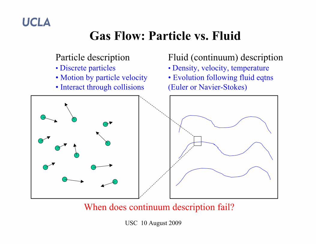
Gas Flow: Particle vs. FluidParticle description• Discrete particles• Motion by particle velocity• Interact through collisions

Fluid (continuum) description• Density, velocity, temperature• Evolution following fluid eqtns(Euler or Navier-Stokes)

When does continuum description fail?

USC 10 August 2009

When Does the ContinuumDescription Fail?

• Rarefied gases and plasmas• Knudsen number Kn=ε

– ε = (mean free path)/(characteristic distance)– measures significance of collisions– mean free path = distance traveled by a particle

between collisions

USC 10 August 2009

Collisional Effects in the Atmosphere

USC 10 August 2009

Rarefied vs. Continuum Flow:Knudsen number Kn

USC 10 August 2009

Collisional Effects in MEMS and NEMS

USC 10 August 2009

Boltzmann equation for rarefied gasdynamics (RGD)

• Statistical description replaces individual particles– density function f=f(x,v,t) in phase space (position x, velocity v) at time t– typical number of 1020 particles would be intractable

• Boltzmann equation for f

– ε = Knudsen number– Q represents effect of binary collisions

• General existence theorem– Diperna & Lions 1989– “renormalized” solution– uniqueness, conservation of energy are not established

1 ( , )t xf v f Q f f! "+ # =�

USC 10 August 2009

Collisions

• Velocities-v,w before collision-v’, w’ after collision

• Conservation of momentum and energy- v + w = v’ + w’- |v|2 + |w|2 = |v’|2 + |w’|2

-Two free parameters- Ω = (ε,θ) on sphere- θ = scattering angle- ε = angle of plane of collision

vv’ w’

w

USC 10 August 2009

Equilibrium and Fluid Limit ofBoltzmann

• Maxwellian equilibrium– Q(f,f) = 0 implies f = M(v;ρ,u,T)

• Equilibration– f=f(v,t) spatially homogeneous– H= - Entropy– Boltzmann’s H-theorem– H-theorem implies f →M as t →∞

• Fluid Limit (Hilbert, Grad, Nishida, REC)– ε→0– f(v,x,t)→ M(v;ρ,u,T), with ρ= ρ(x,t), etc.– ρ,u,T satisfy Euler (or Navier-Stokes)

( ) log( )H f f f dv= !

3 2 2( ) (2 ) exp( ( ) 2 )M T T! " # /= # # /v v u

/ 0dH dt !

USC 10 August 2009

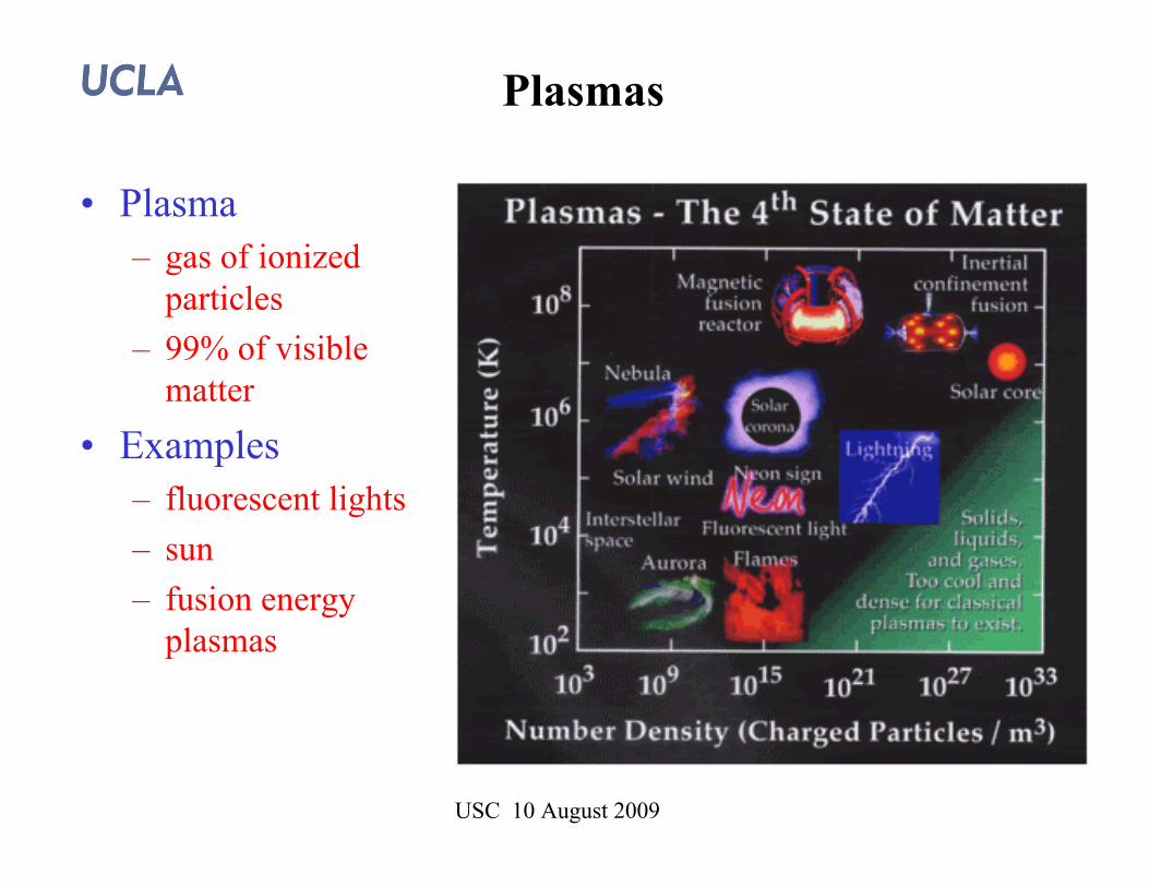
Plasmas

• Plasma– gas of ionized

particles– 99% of visible

matter• Examples

– fluorescent lights– sun– fusion energy

plasmas

USC 10 August 2009

New experimental facilities aredriving plasma physics

• ITER– tokamak (magnetic

confinement fusion)– reactor chamber 840 m3

– originally the InternationalThermonuclear ExperimentalReactor

– international (China, EU,India, Japan, Korea, Russia,US)

– located in southern France

USC 10 August 2009

Scrape-offlayer

Kinetic

Effects

Edge pedestal temperature profile near theedge of an H-mode discharge in the DIII-Dtokamak. [Porter2000]. Pedestal is shadedregion.

Schematic views of divertor tokamak and edge-plasma region (magneticseparatrix is the red line and the black boundaries indicate the shape ofmagnetic flux surfaces)

Where are collisions signifiant in plasmas?Example: Tokamak edge boundary layer

R (cm)

Tem

p. (e

V)

0

500

1000

From G. W. Hammett, review talk 2007 APS Div Plasmas Physics Annual Meeting, Orlando, Nov. 12-16.

USC 10 August 2009

Interactions of Charged Particlesin a Plasma

• Boltzmann equation for plasma with collisions

• Long range interactions– r > λD (λD = Debye length)– Electric and magnetic fields E, B

• Short range interactions– r < λD– Coulomb “collisions”

1 ( )x EM v col

EM

f fv f m F f

t t

v BF q E

c

!" "+ #$ + #$ =

" "

%& '= +( )

* +m=mass, q=charge

USC 10 August 2009

Landau-Fokker-Planck equationfor collisions

• Coulomb interactions– collision rate ≈ u-3 for two particles with

relative velocity u• Fokker-Planck equation

21( ) ( ) ( ) : ( ) ( )

2col d

ff f

t

! ! != " +

! ! ! !F v v D v v

v v v�

1 1

( ')( ) 2 '

| ' |d

H fc c d! !

= =! ! "

# vF v v

v v v v

2 2

2 2( ) ( ') | ' | 'G

c c f d! !

= = "! ! ! !

#D v v v v vv v v v

USC 10 August 2009

Derivation of Landau Equation• Linear Boltzmann equation (idealized)

– collision integral

– conservation of mass

• grazing collisions

– derivation of Landau collision operator

( ) ( , ') ( ') ' ( ) ( )Lf v k v v f v dv v f v!= "#

( , ') ( )k v v d v! "=#

2

( , ') ( ' ( ))

( ' ) ( ' ) ( ' )v v

k v v v v v

v v v v v v

!"

!" # " $ "

% & + '

% & + ( & + ( &

( )

( )

( )

2

' '

2

2

( ) ( ' ) ( ') ' ( )

( ) ( )

( )

v v

v v

v v

Lf v v v f v dv f v

f v f v

f v

! " # $ !

! " # !

" #

% & ' + ' & &

= + ' + ' &

= ' + '

(

SIAM 6 July 2009

Derivation of Ratein Fokker-Planck Eqtn

• Binary Coulomb collision– particles with unit charge q, reduced mass µ– relative velocity v0 , displacement b before collision– deflection angle θ– scattering cross section (Rutherford)

2

2

0

tan( / 2)q

v b!

µ=

22

2 2

0

( )2 sin ( / 2)

q

v! "

µ "

# $= % &' (

b

θ

v0

USC 10 August 2009

Comparison F-P to Boltzmann• Boltzmann

– collisions are single physical collisions– total collision rate for velocity v is

∫|v-v’| σ(|v-v’| ) f(v’) dv’

• FP– actual collision rate is infinite due to long range

interactions: σ = (|v-v’| )-4

– FP “collisions” are each aggregation of many smalldeflections

– described as drift and diffusion in velocity space21

( ) ( ) ( ) : ( ) ( )2

col d

ff f

t

! ! != " +

! ! ! !F v v D v v

v v v�

{ }1 1 1 1 1

( )( ) ( ') ( ') ( ) ( ) ( )col

f vf v f v f v f v v v v v d dv

t! "

#= $ $ $

# % %

USC 10 August 2009

Collisions in Gases vs. Plasmas

• Collisions between velocities v and v*– q=| v - v

* | relative velocity

• Gas collisions– hard spheres, σ = cross section area of sphere– collision rate is σ q– any two velocities can collide → smoothing in v

• Plasma (Coulomb) collisions– very long range, potential O(1/r)– collisions are grazing, localized as in Landau eqtn– differential eqtn in v, as well as x,t– waves in phase space– Landau damping (interaction between waves and particles)

USC 10 August 2009

Dominant numerical method for dilute flows

• DSMC = Direct Simulation Monte Carlo– Invented by Graeme Bird, early 1970’s– Represents density f as collection of particles

– Directly simulates RGD by randomizing collisions• Collision v,w →v’,w’ conserving momentum, energy• Random choice of collision angles (ε,θ)

– Particle advection– Convergence (Wagner 1992)

• Limitation of DSMC– DSMC becomes computationally intractable near fluid

regime, since collision time-scale becomes small

1

( ) ( ( )) ( ( ))N

k k

k

F v v v t x x t! !=

= " "#

/k k

dx dt v=

USC 10 August 2009

Monte Carlo Particle Methodsfor Coulomb Interactions

• Particle-field representation– Mannheimer, Lampe & Joyce, JCP 138 (1997)– Particles feel drag from Fd = -fd (v)v and diffusion of

strength σ = σ(D)

– numerical solution of SDE, with Milstein correction• Lemons et al., J Comp Phys 2008

• Particle-particle representation– Takizuka & Abe, JCP 25 (1977), Nanbu. Phys. Rev. E. 55

(1997) Bobylev & Nanbu Phys. Rev. E. 61 (2000)– Binary particle “collisions”, from collision integral

interpretation of FP equation

dd dt d= +v F ó b

USC 10 August 2009

What can mathematics contributeto DSMC?

• Traditionally, math contributed little toDSMC– only difficulties are computational complexity– no stability, consistency issues

• Flows near fluid limit– DSMC becomes intractable– math needed to design methods that overcome

this difficulty!

USC 10 August 2009

Current Multiscale Methods:What’s New?

• Current multiscale methods– e.g. quasi-continuum, HMM, equations-free method– combine multiple scales and multiple physics into a single

numerical method• Multiscale methods for dilute fluids and plasmas

– applicable in near fluid regime– combine fluid and particle descriptions– provide considerable acceleration over traditional methods– For Coulomb collisions second source of multiscale

behavior is v dependence of cross rate

USC 10 August 2009

Accelerated Simulation Methodsfor Coulomb collisions

• δf methods: f = M + δf– simulate (small) correction to approximate result (Kotschenruether 1988)– δf can be positive or negative– Particle weights: “quiet” and partially linearized methods (Dimits & Lee

1993)– Stability problems

• Hybrid method with thermalization/dethermalization– Hybrid representation (as in RGD)

• m = equilibrium component (Maxwellian)• g = kinetic (nonequilibrium) component

– Thermalization rate must vary in phase space• α = α(x,v) = fraction of particles in m• (um, Tm) ≠ (uF, TF)

( )F v m g= +

USC 10 August 2009

Thermalization/Dethermalization Method

• Hybrid representation (as in RGD)

• Thermalization and dethermalization (T/D)– Thermalize particle (velocity v) with probability pt

• Move from g to m– Dethermalize particle (velocity v) with probability pd

• Move from m to g– Derivation?

( )F v m g= +

USC 10 August 2009

Hybrid collision algorithm

• Hybrid representation (as in RGD)

– g represented by particles

• Collisions– m-m: leaves m unchanged– g-g: as in DSMC– m-g: select particle from g, sample particle from m, then perform

collision• T/D step

– Particle from g is thermalized (moved to m) with probability pt

– Particle sampled from m is dethermalized (moved to g) withprobability pd

• Change (ρm, um, Tm) to conserve mass, momentum, energy

( )F v m g= +

1

( ( ))n

k

k

g v v t!=

= "#

USC 10 August 2009

Choice of Probabilities pd and pt• T/D step

– Fn = F(n dt) = mn + gn– One step

• Detailed balance requirement (?)

– Assuming uM = um = 0• Simple choice

– pt = 1 for v < v1 (i.e., complete thermalization)– pd = 1 for v > v2 (i.e., complete dethermalization)

1 0 0

1 0 0

(1 )

(1 )

d t

d t

m p m p g

g p m p g

= ! +

= + !

0 1

2

(1 )

( / )

(1 / )

(1 / ) exp( / )

d t

d t

d t

d t

F M m g F M m g

g p m p g

g p p m

M p p m

p p c v !

= = + " = = +

# = + $

# =

# = +

# + =

USC 10 August 2009

Application to Bump-on-TailProblems

• Bump-on-tail– central Maxwellian m– bump on tail of m

• Dynamics– fast interactions

• with small |v-v’|• m with m• bump with bump• describe with MHD

– slow interactions• with large |v-v’|• bump with m• describe with particle

collisions

USC 10 August 2009

Hybrid Method for Bump-on-Tail

USC 10 August 2009

Efficiency vs. Accuracy forHybrid Method

USC 10 August 2009

Ion Acoustic Waves

– kinetic descriptionneeded for ionLandau damping andion-ion collisions

– wave oscillation anddecay shown at right

– agreement with“exact” solutionfrom Nanbu

Nanbu ( ), hybrid ( ), older hybrid method ( )

USC 10 August 2009

Hybrid Method Using Fluid Solver• Improved method for spatial inhomogeneities

– Combines fluid solver with hybrid method• previous results used Boltzmann type fluid solver

– Euler equations with source and sink terms fromtherm/detherm

– application to electron sheath (below)• potential (left), electric field (right)

USC 10 August 2009

Generalization of Hybrid MethodHybrid representation using two temperatures

– Tparallel, Ttransverse– anisotropic Maxwellian

– temperature evolution follows Trubnikov solution for relaxation of anisotropy– application to bump-on-tail below

• temperature evolution (left), velocity distribution (right)

3/2 2 1/2 2 2 2( ) (2 ) ( ) exp( ( ) / / )t p x y t z pf v T T v v T v T! " "= " + "

USC 10 August 2009

Conclusions and Prospects

• Lots of opportunities for mathematics inplasma physics

• Current simulation methods for kinetics havetrouble in the fluid and near-fluid regime

• Math leading to new methods that are robust influid limit