Multiscale Gradient Computation for Subsurface Flow Models · Multiscale Gradient Computation for...

ECMOR XV - 15th European Conference on the Mathematics of Oil Recovery

29 August – 1 September 2016, Amsterdam, Netherlands

We Gra 05Multiscale Gradient Computation for SubsurfaceFlow ModelsR. Moraes* (Delft University of Technology), J.R.P. Rodrigues (Petrobras),H. Hajibeygi (Delft University of Technology) & J.D. Jansen (DelftUniversity of Technology)

SUMMARYWe present an efficient multiscale (MS) gradient computation that is suitable for reservoir managementstudies involving optimization techniques for, e.g., computer-assisted history matching or life-cycleproduction optimization. The general, algebraic framework allows for the calculation of gradients usingboth the Direct and Adjoint derivative methods. The framework also allows for the utilization of any MSformulation in the forward reservoir simulation that can be algebraically expressed in terms of a restrictionand a prolongation operator. In the implementation, extra partial derivative information required by thegradient methods is computed via automatic differentiation. Numerical experiments demonstrate theaccuracy of the method compared against those based on fine-scale simulation (industry standard).



Introduction Model-based reservoir management techniques typically rely on the information provided by derivatives. For instance, in sensitivity analysis studies, derivatives can be directly used to identify the most influential parameters in the reservoir responses. Also, derivative information can be utilized in history matching (Oliver and Chen 2011) and control optimization (Jansen 2011) studies, where gradient-based optimization techniques are employed in the minimization/maximization of an objective function.

Such types of model-based reservoir management studies are computationally demanding exercises. They require multiple evaluations of the reservoir model in order to compute its response under the influence of different inputs. Reduced-order modelling (ROM) techniques have been employed to reduce the computational cost of the reservoir response evaluation. On the sensitivity analysis realm, response surface models and design of experiments are often used with this aim (see e.g. Yeten et al. 2005). In history matching and optimization studies, techniques like upscaling (Durlofsky 2005), streamline simulation (Datta-Gupta and King 2007), and proper orthogonal decomposition (Jansen and Durlofsky 2016) are employed to create reservoir models that are faster to evaluate. However, ROM and upscaling methods usually do not provide accurate enough system responses due to excessive simplifications of the fluid-rock physics and heterogeneous geological properties.

Multiscale (MS) methods (Hou and Wu 1997; Jenny et al. 2003; Efendiev and Hou 2009), however, solve a coarser simulation model, thus increasing the computational speed up, while still utilizing features of the fine scale heterogeneous nonlinear simulation model. This provides an efficient and accurate solution of the reservoir model. MS methods are accurate because they honor the high-resolution data using locally computed and adaptively updated basis functions. Important is that the coarse-scale solutions are mapped into the original high-resolution fine scale, using the basis functions. As such, errors can be calculated against the fine-scale reference systems (and not upscaled averaged ones). This allows for development of convergent iterative MS procedures (Hajibeygi et al. 2008, Zhou and Tchelepi 2012). Recent developments include MS formulations for fractured media (Tene et al. 2016) with compositional effects (Hajibeygi and Tchelepi 2014, Kozlova et al. 2015) and complex well configurations (Jenny and Lunati 2009). In addition, algebraic formulation of the method has made it convenient to integrate it within existing simulators using structured (Wang et al. 2014) and unstructured (Shah et al. 2016) grids. The method has been also extended to fully-implicit formulations where all unknowns cross multiple dynamically-defined scales (Cusini et al. 2016). Although these developments are found efficient, they are mainly limited to forward simulation modeling. Of high importance is to integrate the MS methods within reservoir management workflows.

From the derivative calculation techniques perspective, the most traditional approaches are either computationally expensive or inaccurate. For instance, numerical differentiation (see, e.g., Oliver et al. 2008 and Heath 2002) suffers from discretization approximations and truncation errors, and is impractical when the number of parameters is large. Alternatively, analytical methods – Direct Methods and Adjoint Methods (Chen et al. 1974, Chavent et al. 1975) – can provide accurate and efficient derivatives under the appropriate conditions (to be further discussed in the Derivation of the Multiscale Gradient Computation Mathematical Framework section). However, the use of Adjoint Methods has not been extensively adopted mainly because they are code-intrusive and require a substantial implementation effort. Younis and Aziz (2007) discuss how automatic differentiation can partly alleviate the burden of computing derivative information. However, most commercial simulators do not provide analytical derivative capabilities nor do they provide access to extend their functionality in this direction. Partially due to these drawbacks, ensemble methods such as the Ensemble Kalman Filter (EnKF) have become very popular in the data assimilation community



(Aanonsen et al. 2009). Similarly, stochastic approximate gradient techniques such as ensemble optimization (EnOpt) and the stochastic simplex approximate gradient (StoSAG) method are increasingly being used for life cycle optimization (Chen et al. 2009, Fonseca et al. 2016). These methods, however, by design, provide an approximation of the gradient.

The multiscale gradient computation has been studied in the past. In the work of Fu et al. (2010) a Multiscale Adjoint (MSADJ) method is applied to sensitivity computation, where a partitioning of the fine-scale problem is employed, using the same concepts that support the Multiscale Finite Volume forward simulation techniques. The global adjoint problem is solved via a set of coupled sub-grid problems described at a coarser scale. The coarse-scale sensitivities are then interpolated to the local fine grid by reconstructing the local variability of the model parameters with the aid of solving embedded adjoint sub-problems. In a follow up paper, Fu et al. (2011) show that their MSADJ method can be efficiently applied to inverse problems of single-phase flow in heterogeneous porous media. Krogstad et al. (2011) developed an adjoint model for a multiphase flow solver based on a Multiscale Mixed Finite Element formulation. Both pressure and saturations are solved at coarse scale. They demonstrate their method for optimization of the controls settings. As opposed to the work of Fu et al. (2011), the method presented by Krogstad et al. (2011) does not require fine grid quantities. Very good computational performance is reported in their paper for water flooding optimization of relatively big models.

The present development introduces a mathematical framework to compute sensitivities/gradients in a multiscale strategy. The framework enables the same computational efficiency as the methods proposed by Fu et al. (2011) and Krogstad et al. (2011). However, its formulation allows for full flexibility with respect to the types of gradient information that are required by the different model-based reservoir management studies. This is achieved via a self-contained elementary derivation performed via an implicit differentiation strategy, as opposed to the more traditional Lagrange multiplier formulation. Also, the formulation naturally provides not only the Adjoint Method, but also the Direct Method. It is important to note that, although in this work the multiscale finite volume (MSFV) is being studied, the proposed MS-gradient method is not restricted to a specific MS method. Instead, it can be utilized in combination with any MS (and multi-level) strategy that is expressed in terms of restriction and prolongation operators.

This paper is structured as follows. First, the multiscale gradient computation method is derived based on the MS reservoir model equations and the respective model responses. The computation of the required prolongation (matrix of basis functions) operator derivatives is developed within the Multiscale Finite Volume (MSFV) formulation. Thereafter, the Numerical Experiments section describes a systematic investigation of the validation, robustness, and accuracy of the MS-gradient method for test cases of increasing complexity. Because the proposed method is quite fundamental, the experiments are aimed to evaluate the gradient computation itself, rather than any specific application.

Derivation of the Multiscale Gradient Computation Mathematical Framework

Forward Simulation Model We start the derivation of the forward simulation model’s response with respect to the parameters by firstly describing its equations in a generic, purely algebraic form. We restrict the analysis to time-independent (quasi steady-state) problems. In that case, the set of equations that describes the forward simulation at the fine scale can be expressed, without any assumption regarding the underlying physical model, as

,Fg x θ 0 , (1)



where : F FN N NFg F FN N NF FNN represents the set of algebraic simulator equations, FNx FNF is the state vector (which, for single-phase flow, contains the grid block pressures), Nθ NNN is the vector of parameters (which typically contains grid block permeabilities and porosities but possibly also other parameters such as fault transmissibility multipliers or structural parameters), and the subscript F refers to ‘fine scale’. There are FN fine-scale cells and N parameters. Eq. (1) implicitly assumes a dependency of the state vector x on the parameters θ , i.e.,

x x θ . (2)

Once the model state is determined, the observable responses of the forward model are computed. The forward model responses (typically wellbore pressures and/or rates) may not only depend on the model state, but also on the parameters themselves, and can be expressed as

,F Fy h x θ , (3)

where : yF NN NFh yF NyN NF NNN represents the output equations (Jansen 2013a). It is assumed that Fg can be described as

,Fg x θ A θ x q θ , (4)

where ( )A θ is an F FN N matrix and ( )q θ is an FN vector.

Algebraic Multiscale Formulation of Subsurface Flow in Heterogeneous Porous Media MS methods provide accurate and efficient solutions to the flow equations by incorporating the fine-scale heterogeneities in a coarse-scale operator (Hajibeygi 2011). This is achieved by basis functions, which are local solutions of the governing equations without right-hand-side (RHS) terms, subject to assumed local boundary conditions. These local basis functions construct the prolongation (interpolation) operator, ( )P P θ , which is an F CN N matrix responsible to map (interpolate) the coarse-scale solution to the fine-scale resolution (Zhou and Tchelepi 2008). For the purpose of the development here presented, the required basic knowledge about the multiscale strategy is that a coarse-scale system can be algebraically described once the restriction operator, ( )R R θ , is defined as an C FN N matrix which maps the fine scale to the coarse scale (more information can be found in Wang et al. 2014). Let CNxx CNC be the coarse scale solution ( C FN NFNF ), ( )R R θ be an C FN N matrix mapping from the fine scale to the coarse scale and ( )P P θ be an F CN N matrix mapping from the coarse scale to the fine scale. R and P will be referred to as the restriction and prolongation operators, respectively. xx is obtained by solving

g RAP x Rq Ax q 0g RAP xx Rq Ax q 0x Rq Ax q 0Ax q 0 . (5)

Finally, the approximated fine-scale solution x is obtained by interpolating the coarse scale solution xx , i.e.,

x Pxx . (6)

Derivative Calculation of Simulator Responses In order to derive an expression to compute the derivatives of the responses obtained by the multiscale method with respect to the parameters, we follow a formulation similar to the one that has been used by Rodrigues (2006) and Kraaijevanger et al. (2007). This formulation can be interpreted as a form of implicit differentiation and is equivalent to the standard Lagrange multiplier formulation (Jansen 2016). However, unlike the Lagrange multiplier formulation, this approach does not depend on a particular objective function and naturally provides both the Direct and the Adjoint Methods, as well as algorithms for multiplying the sensitivity matrix and its transpose with arbitrary vectors.



We define g , the function that describes the approximate primary variables solution at the fine scale from Eq. (6) as

g x Px 0x 0 . (7)

The state vector can now be described as the combination of both sets of primary variables in the fine and coarse scales, i.e.,

x

xx

, (8)

and, similarly, the model equations being the combination of the equations at both scales, i.e.,

,g

g x θ 0g

. (9)

By defining the state vector as in Eq. (8), we allow for the ability to describe the state not only at the fine scale, but at the coarse scale as well. This definition is a key aspect of the formulation. The simulator responses y obtained from the multiscale method are represented as

,y h x θ . (10)

The sensitivity matrix G is then computed by obtaining the derivative of Eq.(10) with respect to θ as

d dd dh h x hGθ x θ θ

. (11)

In order to find a relationship that defines the derivative of the state vector with respect to the parameters, we differentiate Eq. (9) with respect to θ

dd

g x g 0x θ θ

, (12)

so that

1d

dx g gθ x θ

. (13)

Substituting Eq. (13) in Eq. (11) gives

1h g g hG

x x θ θ. (14)

From Eqs. (5), (7), (8) and (9), it follows that

RAP 0g

P Ix. (15)

Note that

1 1

1

( )

( )

RAP 0gx P RAP I

(16)

holds. Thus, Eq. (14) can be restated as

1h h g h g hG P RAP

x x θ x θ θ. (17)



By deriving Eq. (5) with respect to θ one finds

g R A P R qAP R P RA x q Rθ θ θ θ θ θ

(18)

and also, from Eq. (7),

g P xθ θ

x . (19)

Note that the partial derivatives of the matrices A , R and P with respect to the vector of parameters θ result in (third order) tensors. The tensors (and the operations with them) can be fully expressed using the Index notation. The substitution of Eqs. (18) and (19) in Eq. (17) leads to the expression that will serve as the basis for the multiscale gradient computation, i.e.,

1h h R A P R q h P hG P RAP AP R P RA x q R xx x θ θ θ θ θ x θ θ

h (20)

Eq. (20) is quite general, i.e., it can be employed to compute gradients for any MS (and multi-level) method, given that the partial derivatives of R and P are provided.

For the sake of simplicity and to be coherent with the numerical experiments herewith presented, from now on we neglect the dependency of the restriction operator R and the right-hand-side vector q on the parameters. This is consistent with the MSFV method (where the restriction operator is based on a finite volume integration operator at coarse scale (see e.g. Wang et al. 2014). After these simplifications, Eq. (20) can be rewritten as

1h h A P h P hG P RAP R P A x x

x x θ θ x θ θh

. (21)

The order of the operations involved in 1( )RAP term is crucial to determine the computational performance of the sensitivity matrix computation. This order defines two different algorithms known in the literature as the Direct and Adjoint Methods. The following sections discuss how the two methods are derived for the MS scenario defined by Eq. (21), as well as the (dis)advantages of utilizing each of them.

Computation of Gradient Information: Generalization of the Framework According to the type of study one wants to perform, different derivative information has to be provided. For instance, for optimization methods, Quasi-Newton methods require the gradient of the objective function (and possibly constraints). In history matching algorithms, as well as in sensitivity analysis studies, the sensitivity matrix G plays an important role. In Gauss-Newton methods, matrix

TG G is directly used, while conjugate gradient methods require products of G and TG with arbitrary vectors. Nocedal and Wright (2006) provide more detailed information on the different optimization algorithms.

To preserve general applicability of our method, we consider the general problem of multiplying G by arbitrary matrices W (of order Ym N ) and ( V of order N n ) from left and right, respectively. When 1n , GV is simply the product of G with a vector, whereas, when 1m , ( )T T TWG G W gives the product of TG with the (column) vector TW . Those examples show how, by defining algorithms to calculate GV and WG for arbitrary V and W , different types of derivative information can be accommodated in a single framework.



Direct Method We start by considering the calculation of GV for a given N n matrix V . From Eq. (21), by defining

1 A PZ RAP R P A x Vθ θ

V , (22)

the product GV can be rewritten as

h h h P hGV P Z x V Vx x x θ θ

hV h (23)

Here, Z is obtained as the solution to the following linear system of equations

A PRAP Z R Px A x Vθ θ

V . (24)

This is known as the Forward Method (Rodrigues 2006) or Direct Method (Oliver et al. 2008). Note that Z has dimensions of CN n and, therefore, it requires n linear systems to be solved. Hence, the cost of computing GV is proportional to the number of columns in V . In particular, to obtain the full sensitivity matrix G with the Direct Method, in which case one has to set V equal to the identity matrix of order N , the cost will be proportional to the number of parameters.

Adjoint Method Next we consider the calculation of WG for a given Ym N matrix W . From Eq. (21), defining

1T h hZ W P RAPx x

, (25)

one obtains

T A P h P hWG Z R P A x W x Wθ θ x θ θ

hx W x W , (26)

which can be rearranged as

T TA h P hWG Z R Px Z RA W x Wθ x θ θ

hT WTTTTTTTT . (27)

Multiplying Eq. (25) by RAP from the right and transposing, Z is obtained as the solution to the following linear system of equations

T

T Th hRAP Z P Wx x

. (28)

This is known in the literature as the Adjoint (or Backward) Method (Chavent et al. 1975). Note that now Z has dimensions of CN m , hence it requires m linear systems to be solved. As such, the cost of computing WG is proportional to the number of rows in W . In particular, to obtain the full sensitivity matrix G with the Adjoint Method, in which case one has to set W equal to the identity matrix of order YN , the cost will be proportional to the number of responses.

Partial Derivative Computation and Automatic Differentiation In the computation of analytical gradients, a significant part of the overall implementation effort is associated with the computation of partial derivative matrices. This computation step often requires access to the source code because not all partial derivatives are readily available, as opposed to the



state variable derivatives via the Jacobian matrix. To calculate the partial derivative matrices an Automatic Differentiation (AD) approach is used, because of its flexibility and accuracy. A review of different AD approaches is provided by Younis et al. (2007). In our work, an Operator Overloading AD technique (Bendtsen and Stauning 1996) based on Expression Templates (Vandevoorde and Josuttis 2003) is applied. This facilitates the computation and assemblage of all the partial derivative matrices because they are obtained at the same time the system matrix A and the simulator response y are computed.

Partial Derivative of MSFV Prolongation Operator with Respect to the Parameters A particular aspect of the methodology is the computation of partial derivatives of the prolongation operator with respect to the parameters, i.e., ( P θ ) in Eq. (21), and operations with this tensor. This is particularly challenging because the computation of P might involve complex operations, e.g., the solution of linear systems in the case of MSFV methods.

In this work, we consider the MSFV method; extension to other MS methodologies can be obtained along the same lines. In this case, P is the assembly of all basis functions obtained via the solution of local flow problems, i.e.,

0 (29)

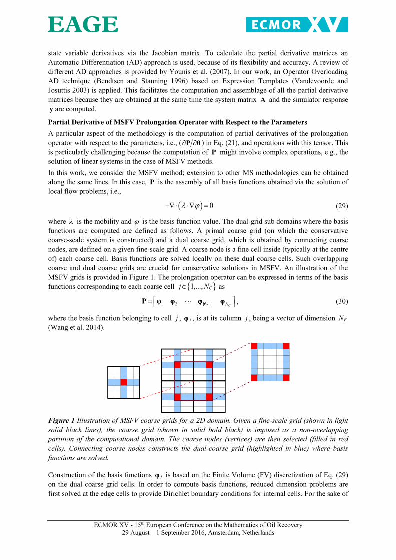
where is the mobility and is the basis function value. The dual-grid sub domains where the basis functions are computed are defined as follows. A primal coarse grid (on which the conservative coarse-scale system is constructed) and a dual coarse grid, which is obtained by connecting coarse nodes, are defined on a given fine-scale grid. A coarse node is a fine cell inside (typically at the centre of) each coarse cell. Basis functions are solved locally on these dual coarse cells. Such overlapping coarse and dual coarse grids are crucial for conservative solutions in MSFV. An illustration of the MSFV grids is provided in Figure 1. The prolongation operator can be expressed in terms of the basis functions corresponding to each coarse cell 1,..., Cj N as

1 2 1C CN NP φ φ φ φCNC 11111 , (30)

where the basis function belonging to cell j , jφ , is at its column j , being a vector of dimension FN (Wang et al. 2014).

Figure 1 Illustration of MSFV coarse grids for a 2D domain. Given a fine-scale grid (shown in light solid black lines), the coarse grid (shown in solid bold black) is imposed as a non-overlapping partition of the computational domain. The coarse nodes (vertices) are then selected (filled in red cells). Connecting coarse nodes constructs the dual-coarse grid (highlighted in blue) where basis functions are solved.

Construction of the basis functions jφ is based on the Finite Volume (FV) discretization of Eq. (29) on the dual coarse grid cells. In order to compute basis functions, reduced dimension problems are first solved at the edge cells to provide Dirichlet boundary conditions for internal cells. For the sake of



clarity, let us assume a Cartesian two-dimensional solution domain (although extension to 3D is straightforward) More specifically, let j be the set of all edges emanating from coarse node j (in 2D, # 4j ). For each edge je , let

, , ,E E Ee j e j e jA φ b 0 (31)

be the reduced-dimension discrete form of Eq. (29) along the edge e , where ,Ee jφ is the basis function

at that edge, and ,Ee jb is the RHS which results from specifying corner values of , 1E

e j at the vertex j and , 0E

e j at the opposite vertex of e . If j is the set of all faces which have coarse node j as a common vertex ( # 4j in 2D), for each face jf , according to Eq. (29), one can solve

, , , ,

j

F F F Ef j f j e f e j

eA φ E φ 0 , (32)

for ,Ff jφ , which is the basis function at the internal (face) cells. Also, ,

Fe fE is a transformation matrix

that appropriately assembles a vector represented in the edge topology of e into the face topology of f . Finally, jφ is the result of assembling the contribution of each ,

Ff jφ , jf , into the overall fine

mesh topology:

,

j

Fj f f j

fφ E φ , (33)

where fE is a transformation matrix that assembles a vector represented in the face topology of f into a size FN vector following the fine grid topology.

The derivative of jφ w.r.t. the parameters is obtained from Eq. (33), i.e.,

,

j

Fj f j

ff

φ φE

θ θ. (34)

Differentiating Eq. (32), one can write

1, , ,

, , ,

j

F F Ef j f j e jF F F

f j f j e fe

φ A φA φ E

θ θ θ. (35)

Similarly, from Eq. (31),

1, ,

, ,

E Ee j e jE E

e j e j

φ AA φ

θ θ (36)

holds. Combining Eqs. (35) and (36) into (34) results in

1 1, ,

, , , , ,

j j

F Ej f j e jF F F E E

f f j f j e f e j e jf e

φ A AE A φ E A φ

θ θ θ. (37)

The third order tensor defining the derivative of P w.r.t. the parameters is obtained by grouping all

jφ θ at its slices,

11 2 C C

F C

N N

N N N

φ φφ φPθ θ θ θ θ

CNCNNNCNC . (38)

P θ is a F CN N N third order tensor that can be interpreted as a stack of N matrices of partial derivatives jφ θ , 1,..., Cj N , each of dimension F CN N . As part of the computation of the Direct Method the product ( )P θx m)m) is required, where CNxx CNC and Nm NNN . Since



1

CNj

jj

φP x xθ θ

CNCj

j

φxjx , (39)

where jx jx denotes the j-th entry of vector xx , it follows, from (37), that

1 1, ,

, , , , ,1

C

j j

F ENf j e jF F F E E

j f f j f j e f e j e jj f e

A AP x m x E A φ m E A φ mθ θ θ

CNCFffm j ffff . (40)

In a similar manner, as part of the computation of the Adjoint Method, the product ( )Tm P θx) is required, where CNxx CNC and FNm FNF . From Eqs. (37) and (39), one obtains

1 1, ,

, , , , ,1

C

j j

F ENf j e jT T F F F E E

j f f j f j e f e j e jj f e

A APm x x m E A φ E A φθ θ θ

CNCTTT

j ff . (41)

Numerical Experiments In this section, a systematic performance study for the MS-gradient method is presented for single-phase incompressible flow in heterogeneous porous media. Because this is the scenario for which the MS methods were originally developed, it provides a simple, yet effective, way to validate the derivative calculation methodology proposed in this work.

The following numerical experiments are presented to first validate and then assess the accuracy of the gradient information computed by the method. For this purpose, a misfit objective function with no regularization term

11, ,

2

Tobs D obsO θ h x θ d C h x θ d , (42)

with a gradient

1 ,TD obsOθ G C h x θ d , (43)

is considered (Oliver et al. 2008). In all experiments, the fitting parameters are cell-centered permeabilities and the observed quantity is the fine scale pressure at the location of observation wells. Therefore there is no explicit dependency of the response on the parameters, i.e.,

h Ix

, (44)

and

h 0xh 0x

. (45)

The tensor A θ represents partial derivatives of the system (transmissibility) matrix with respect to permeability.

Wells and other source terms are considered by supplementary well basis functions (Jenny and Lunati 2009; Tene et al. 2016). Well functions are local solutions of the Eq. (29) considering a unit solution at the well location and zero values at the coarse nodes. Hence, considering well functions, the prolongation operator (for porous rock) is enriched and reads

1 1|C WN NP φ φ ψ ψ|C WN NC W1| N111| 1 , (46)

where each well function wψ adds a column vector to the porous rock prolongation operator. Note that there are WN wells in the domain. For rate-constrained wells, one has to add additional rows to



the prolongation (and consequently, the coarse-scale system) in order to solve for the well pressures as additional unknowns (Jenny and Lunati 2009 and Tene et al. 2016). The derivative of Eq. (46) w.r.t. the parameters is given by

1 1|C WN Nφ ψφ ψPθ θ θ θ θ

N1| W1 W1 WNW| 1111NN || . (47)

The computation of well basis function partial derivatives follows the solution strategy discussed for Eq. (37). In all the following test cases, well basis functions are included.

Validation Experiments The MS-gradient method is validated against the numerical differentiation method for a higher-order, two-sided Taylor approximation of

1 1

1, , , , , , , , , , , ,

2i i i i i i i N i i i i i i Ni

O O Oθ i i i i i N i i i i N, , , , , , , , , , ,, , , , , , , ,N i i i i i i NN i i i i N, ,i i ii , , ,O1, , , , , , , ,,, , , , , , , ,1 1i i i i i1, ,,1 ,1 i1,1O1i 1, 1 ,11 , (48)

where is a multiplicative parameter perturbation. The relative error can be defined as

2

2

FD AN

AN

O OO

θ θ

θ

, (49)

where FDOθ is obtained by performing the appropriate number of multiscale reservoir simulations required to evaluate Eq. (48) and ANOθ is obtained by either employing the Direct or Adjoint Method to evaluate Eq. (43). Note that

1 ,D obsm C h x θ d , (50)

where m is an auxiliary vector, so the gradient of O can be written as ( )T TOθ m G and Oθ can be calculated with a cost proportional to one extra MS simulation, making the Adjoint Method a much more efficient way to calculate the gradient than the Direct Method. Moreover, it is assumed, for simplicity, DC I .

In order to validate the proposed derivative calculation methods, as well as their implementation, we investigate the linear decrease of the error by decreasing the perturbation value (see chapter 8 of Heath 2002) from 10-1 to 10-4 (the range within which we observe discretization errors only).

The investigation is carried out in two 2D test cases, one homogeneous and another heterogeneous. In both cases the fine grid size is 21x21, while the coarse grid size is 3x3 (coarsening ratio of 7x7). The primal- and dual-coarse grids are illustrated in Figure 2a.

(a) (b)

Figure 2 (a) Fine, primal and dual coarse grids for 2D validation test cases and (b) reference permeability field.

The permeability field is extracted from 1,000 geological realizations, as shown in Figure 2b, and serves to compute the observed pressure. For the heterogeneous case, another geological realization is



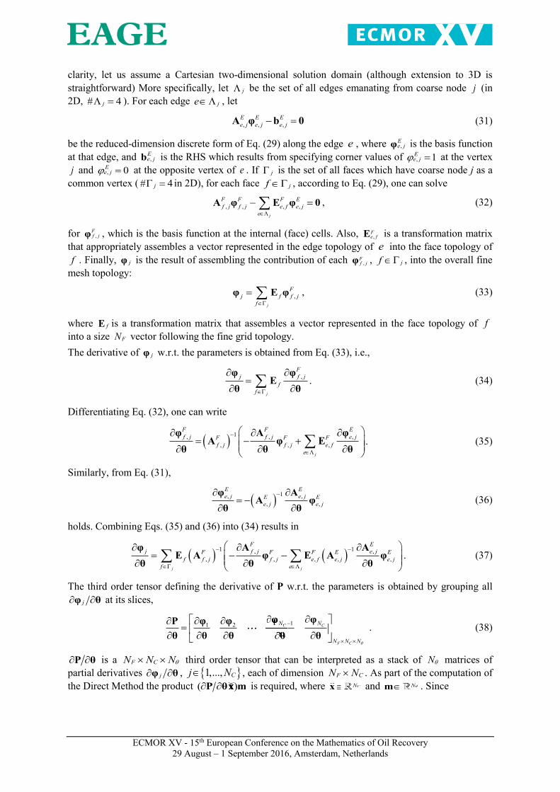
chosen from the ensemble. The ensemble is generated via the decomposition of a reference permeability “image” using Principal Component Analysis parameterization. Figure 3 illustrates 4 different permeability realizations from the ensemble. See Jansen (2013b) for more details.

Figure 3 Four different permeability realizations from the ensemble of 1,000 members used in the 2D numerical experiments.

A quarter five-spot well configuration is considered, with two observation wells close to the operating wells. The well positions and operating pressures are described in Table 1.

Table 1 Well configuration for the homogeneous, two-dimensional case.

Well Fine scale position (I, J) Well type Prescribe

pressure [Pa] INJE (1, 1) Injection 2

PROD (21, 21) Production 1

OBSWELL1 (3, 3) Observation -


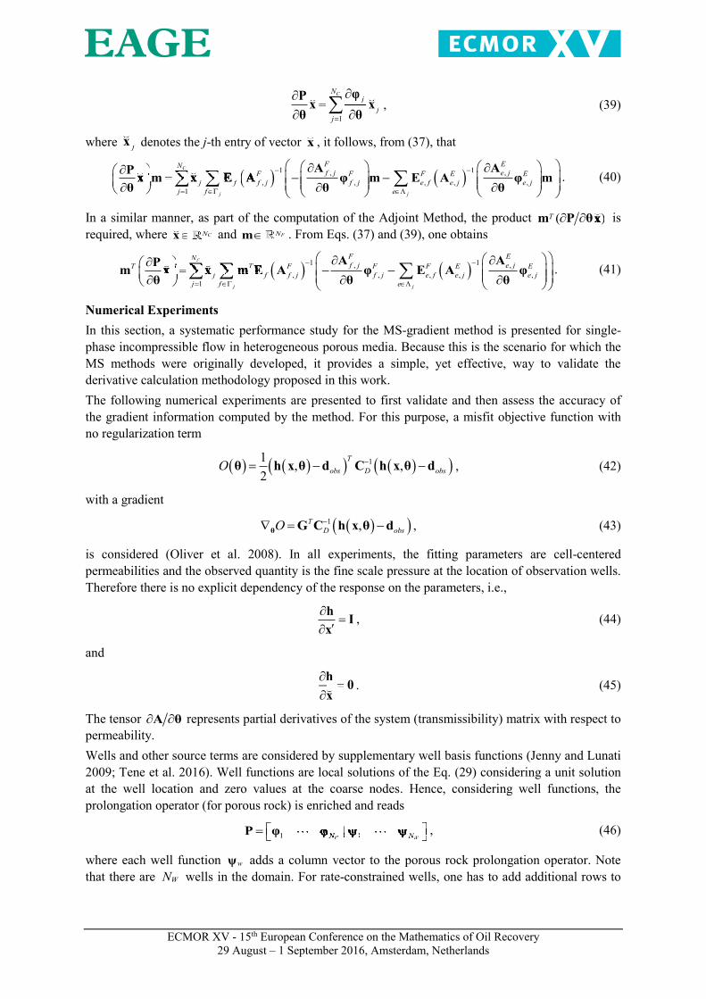
Figure 4 shows that the MS-gradient and fine-scale methods have exactly the same order of accuracy with respect to the perturbation , for all cases. The expected behaviour of linearly decreasing error values as the perturbation size decreases is observed in all experiments. One can also note that the Direct and Adjoint Methods are equally accurate, i.e., they both provide the analytical gradient at the same accuracy.

(a) (b)

Figure 4 Validation of MS gradient computation method via comparison with numerical differentiation: two-dimensional homogenous (a) and heterogeneous (b) steady-state flow test cases.

Gradient Accuracy In order to assess the quality of the MS gradient, the angle between fine-scale and MS normalized gradients, i.e.,

1 ˆ ˆcos TFS MSO Oθ θ , (51)

is measured. Here,



2 2

ˆ ˆ and FS MSFS MS

FS MS

O OO OO Oθ θ

θ θθ θ

. (52)

Also, FSOθ and MSOθ denote the fine-scale and MS analytical gradients, respectively. As a minimum requirement, acceptable MS gradients are obtained if is much smaller than 90o (Fonseca et al. 2015).

For the 2D homogenous case, the fine scale and MS gradients result in 10.97o , using the same setup depicted in Figure 2a. Although the gradients are practically pointing in the same direction, a deviation between the two is observed. To better investigate this difference, Figure 5a and Figure 5b present the fine-scale and MS pressure solutions, respectively, and Figure 5c shows the difference between these two pressure solutions. Figure 5d and Figure 5e present the absolute, normalized gradient of the OF computed via fine-scale and MS gradient methods, respectively. Figure 5f shows the difference between the absolute, normalized gradient computed by the two methods.

(a) (b) (c)

(d) (e) (f)

Figure 5 Fine scale (p) pressure solution (a) and MSFV ( p ) pressure solution (b). Difference between fine-scale and MSFV pressure solutions (c). Absolute, normalized fine scale gradient (d) and MSFV (e). Difference between fine-scale and MS absolute, normalized gradients (f). In both figures the dual-coarse grid is shown. Also shown, in the red boxes, are the coarse nodes.

The difference between the MS and fine-scale methods is due to the localization assumption in the calculation of the basis functions (Hajibeygi et al. 2008). Note that thanks to the well functions, the multiscale solutions are accurately capturing the wells.

Effect of Heterogeneity Distribution In addition to localization assumptions, basis functions are also affected by heterogeneity distribution. In order to explore this point, four sets of 20 equiprobable geostatistical realizations of permeability fields, generated using sequential Gaussian simulations (Remy et al. 2009), are considered. For each set, variance and mean of ln( )k are 2.0 and 3.0, respectively, where k is the grid block permeability. As depicted in Figure 6, for the realizations with a long correlation length, the angles between the permeability layers and the horizontal axis are 0o, 15o, and 45o. A patchy (small correlation length) pattern is also considered (Figure 6d). Compared with the previous set, the permeability contrast is much higher in this case.



(a) (b) (c) (d)

Figure 6 Permeability distribution of four different realizations taken from the sets of 20 geostatistically equiprobable permeability fields with 0o (a), 15 o (b), and 45 o (c) correlation angles. Also, a patchy field (d) with a small correlation length is considered.

The fine-scale and coarse grids contain 100 x 100 and 20 x 20 cells, respectively. The well configuration utilized in this numerical experiment is depicted in Table 2.

Table 2 Well configuration for Case 2.

Well Fine scale position (I, J) Well type Prescribed

pressure [Pa] INJE (1, 1) Injection 2

PROD (100, 100) Production 1



From Figure 7, one can observe that all cases with o50 are associated with small gradient norms and that, for all geological sets, the MS gradient provides gradient directions that are very accurate, compared with the fine scale solution, when the gradient norms are large.

Figure 7 Cross-plot of fine scale gradient norm (log scale) vs. for the four sets of 20 equiprobable permeability realizations.

Note also that, in the case of a small gradient norm, the OF has a weak dependency on the parameters in the vicinity of the point where the gradient is being calculated. As such, the overall performance of the optimization algorithm is not expected to be affected by replacing the fine-scale gradient calculation with the MS version. In general, an iterative multiscale procedure (Hajibeygi et al. 2008) would guarantee high quality MS solutions –to any desired level– for all challenging scenarios. We intend this to be subject of our future research.



Conclusions We developed a Multiscale gradient computation strategy using an algebraic framework that does not depend on a particular objective function. This is possible by recasting the derivative calculation problem as the general problem of multiplying a sensitivity matrix and its transpose with arbitrary matrices. Hence the framework is capable of providing different types of gradient information. Such flexibility allows the employment of the framework to any reservoir management study that requires gradient information. Also, the formulation naturally provides both Direct and Adjoint Methods. The choice between one or the other will depend on the type of derivative information requested, i.e. on the ratio between the number of parameters and the number of derivatives required. Since most of the derivations are expressed in terms of general restriction and prolongation operators, the presented strategy can be applied to all MS (and multilevel) methodologies.

The accuracy of the developed MS gradient computation strategy is studied for a set of examples with increasing complexity. The investigations show that the sources of inaccuracies in the MS solution (e.g. localization assumptions) also result in inaccuracies in the gradient computation. However, fortunately, strategies to improve the MS solution (e.g. well functions) also improve the MS gradient accuracy. Another important observation is the fact that greater angles between MS and fine scale gradient vectors are associated with small values of the gradient norms. Because small gradient norms indicate a weak association between parameters and responses, such differences are typically not very relevant in optimization. All this indicates that the method presented allows for accurate, yet less computationally expensive, gradient computation information that can be successfully utilized in reservoir management studies.

The model calibration examples presented show how the MS gradient computation framework can be employed when the parameters are expressed in the fine scale. The framework allows the computation of fine scale derivative information when the prolongation operator depends on the parameters. By employing the MSFV method as forward simulation technique, partial derivatives of the prolongation operator can be computed via the solution of local problems, similarly to the basis function computation. This allows the demanding computations to be performed only at the coarse scale and in the reduced domains associated with the basis functions computation. Although not shown here, the restriction and prolongation operators may not depend on the parameters (e.g. the parameters being the well controls in a life-cycle optimization study). In this case, the computation of partial derivatives of these operators is not necessary. Therefore, for these scenarios, the utilization of MS gradients is even more advantageous from a computational performance perspective.

The indication that strategies to improve the state variables solution also improve the gradient computation suggests that an iterative MS strategy (Hajibeygi et al. 2008) can be an interesting alternative to obtain more accurate gradients. The algebraic framework here introduced allows for the incorporation of a smoothing step in the gradient computation, to resolve high-frequency errors. We intend this extension to be a subject of our future research.

Finally, the multiscale nature of the method may further benefit data assimilation studies. Various types of data are naturally linked to different spatial scales. Hence, it is not uncommon to upscale/downscale quantities to appropriately fit them into the reservoir simulation model. A multiscale data assimilation strategy, in contrast, allows for the appropriate handling of such types of data with minimum loss of information, due to avoiding the excessively upscaled quantities. This will also be a subject of our future research.

Acknowledgements Rafael Moraes was sponsored by Petrobras S.A. The authors would like to thank the Delft Advanced Reservoir Simulation (DARSim) research team for fruitful discussions during the development of the MS-gradient method.



References Aanonsen, S. I., Nævdal, G., Oliver, D. S., Reynolds, A. C., and Vallès, B. [2009]. The ensemble

Kalman filter in reservoir engineering - a review. SPE Journal, 14(03), 393-412.

Bendtsen C. and Stauning, O. [1996]. FADBAD, a Flexible C++ Package for Automatic Differentiation, Using the Forward and Backward Mehtods (Technical Report IMM-REP-1996-17, Department of Mathematical Modelling, Technical University of Denmark).

Chavent, G., Dupuy, M., and Lemmonier, P. [1975]. History matching by use of optimal theory. SPE Journal, 15 (01), 74-86.

Chen, W.H., Gavalas, G.R. and Wasserman, M.L. [1974]. A new algorithm for automatic history matching. SPE Journal 14(6) 593-608.

Chen, Y., Oliver, D.S. and Zhang, D. [2009]. Efficient ensemble-based closed-loop production optimization. SPE Journal; 14(4) 634-645.

Cusini M., van Kruijsdijk, C., Hajibeygi, H. [2016]. Algebraic dynamic multilevel (ADM) method for fully implicit simulations of multiphase flow in porous media, Journal of Computational Physics, 314, 60-79.

Datta-Gupta, A. and King, M.J. [2007]. Streamline simulation: Theory and Practice, SPE Textbook Series, 11, SPE, Richardson.

Durlofsky, L. J. [2005]. Upscaling and gridding of fine scale geological models for flow simulation. In 8th International Forum on Reservoir Simulation Iles Borromees, Stresa, Italy.

Efendiev, Y., Hou, T. Y. [2009]. Multiscale Finite Element Methods: Theory and Applications, (Surveys and Tutorials in the Applied Mathematical Sciences, Vol. 4), Springer.

Fonseca, R.M., Chen, B., Jansen, J.D. and Reynolds, A.C. [2016]. A stochastic simplex approximate gradient (StoSAG) for optimization under uncertainty. Submitted to International Journal for Numerical Methods in Engineering.

Fonseca, R.M., Kahrobaei, S., Van Gastel, L.J.T., Leeuwenburgh, O., and Jansen, J.D. [2015]. Quantification of the impact of ensemble size on the quality of an ensemble gradient using principles of hypothesis testing. Paper 173236-MS presented at the 2015 SPE Reservoir Simulation Symposium, Houston, USA, 22-25 February.

Fu, J., Tchelepi, H. A., and Caers, J. [2010]. A multiscale adjoint method to compute sensitivity coefficients for flow in heterogeneous porous media. Advances in water resources, 33(6), 698-709.

Fu, J., Caers, J., and Tchelepi, H. A. [2011]. A multiscale method for subsurface inverse modeling: Single-phase transient flow. Advances in Water Resources, 34(8), 967-979.

Hajibeygi, H. [2011]. Iterative multiscale finite volume method for multiphase flow in porous media with complex physics (Doctoral dissertation, Diss., Eidgenössische Technische Hochschule ETH Zürich, Nr. 19872, 2011).

Hajibeygi, H., Bonfigli, G., Hesse, M. A., and Jenny, P. [2008]. Iterative multiscale finite-volume method. Journal of Computational Physics, 227(19), 8604-8621.

Hajibeygi, H., Jenny, P. [2011]. Adaptive iterative multiscale finite volume method, Journal of Computational Physics, 230(6), 628-643.

Hajibeygi, H., Tchelepi, H.A. [2014]. Compositional multiscale finite-volume formulation, SPE Journal 19 (2), 316-326.

Heath, M.T. [2002]. Scientific Computing: An Introductory Survey, 2nd edition, McGraw-Hill.

Hou, T. Y., and Wu, X. H. [1997]. A multiscale finite element method for elliptic problems in composite materials and porous media. Journal of Computational Physics, 134(1), 169-189.

Jansen, J. D. [2011]. Adjoint-based optimization of multi-phase flow through porous media–a review. Computers & Fluids, 46(1), 40-51.

Jansen, J.D. [2013a]. A systems description of flow through porous media. SpringerBriefs in Earth Sciences, Springer.



Jansen, J. D. [2013b]. A simple algorithm to generate small geostatistical ensembles for subsurface flow simulation. (Research Note, TU Delft, Delft University of Technology).

Jansen, J.D. [2016]. Gradient-based optimization of flow through porous media, v.3. Course notes AES1490. Delft University of Technology.

Jansen, J.D. and Durlofsky, L., [2016]. Use of reduced-order models in well control optimization. Optimization and Engineering. Published online. DOI: 10.1007/s11081-016-9313-6.

Jenny, P., Lee, S. H., and Tchelepi, H. A. [2003]. Multi-scale finite-volume method for elliptic problems in subsurface flow simulation. Journal of Computational Physics, 187(1), 47-67.

Jenny, P., & Lunati, I. [2009]. Modeling complex wells with the multi-scale finite-volume method. Journal of Computational Physics, 228(3), 687-702.

Kozlova, A., Li, Z., Natvig, J., Watanabe, S., Zhou, Y., Bratvedt, K. and Lee, S. [2015]. A Real-Field Multiscale Black-Oil Reservoir Simulator. Paper 173226-MS presented at SPE Reservoir Simulation Symposium, 23-25 February, Houston, USA.

Kraaijevanger, J. F. B. M., Egberts, P. J. P., Valstar, J. R., & Buurman, H. W. [2007]. Optimal waterflood design using the adjoint method. Paper 105764-MS presented at the SPE Reservoir Simulation Symposium, 26-28 February, Houston, USA.

Krogstad, S., Hauge, V. L., and Gulbransen, A. [2011]. Adjoint multiscale mixed finite elements. SPE Journal, 16(01), 162-171.

Nocedal, J., & Wright, S. [2006]. Numerical optimization. Springer Science & Business Media.

Oliver, D. S., Reynolds, A. C., and Liu, N. [2008]. Inverse theory for petroleum reservoir characterization and history matching. Cambridge University Press.

Oliver, D. S., and Chen, Y. [2011]. Recent progress on reservoir history matching: a review. Computational Geosciences, 15(1), 185-221.

Remy, N., Boucher, A., and Wu, J. [2009]. Applied Geostatistics with SGeMS: A User’s Guide, Cambridge University Press, New York.

Rodrigues, J. R. P. [2006]. Calculating derivatives for automatic history matching. Computational Geosciences, 10(1), 119-136.

Sarma, P., Aziz, K., and Durlofsky, L. J. [2005]. Implementation of adjoint solution for optimal control of smart wells. Paper 92864-MS presented at the SPE Reservoir Simulation Symposium, 31 January-2 February, The Woodlands, USA.

Shah, S., Moyner, O., Tene, M., Lie, K-A., Hajibeygi, H [2016]. The multiscale restriction smoothed basis method for fractured porous media (F-MsRSB),Journal of Computational Physics,318,36-57.

Tene, M., Al Kobaisi, M.S., Hajibeygi, H. [2016]. Algebraic multiscale method for flow in heterogeneous porous media with embedded discrete fractures (F-AMS), Journal of Computational Physics, in press, DOI: 10.1016/j.jcp.2016.06.012.

Vandevoorde, D. and Josuttis, N. M. [2003]. C++ Templates: The Complete Guide. Addison-Wesley Professional.

Wang, Y., Hajibeygi, H., and Tchelepi, H. A. [2014]. Algebraic multiscale solver for flow in heterogeneous porous media. Journal of Computational Physics, 259, 284-303.

Yeten, B., Castellini, A., Guyaguler, B., and Chen, W. H. [2005]. A comparison study on experimental design and response surface methodologies. Paper 93347-MS presented at the SPE Reservoir Simulation Symposium, 31 January-2 February, The Woodlands, USA.

Younis, R., and Aziz, K. [2007]. Parallel automatically differentiable data-types for next-generation simulator development. Paper 106493-MS presented at the SPE Reservoir Simulation Symposium, 26-28 February, Houston, USA.

Zhou, H. and Tchelepi, H.A. [2008]. Operator-based multiscale method for compressible flow. SPE Journal, 13(2), 523–539.

Zhou, H. and Tchelepi, H.A. [2012]. Two-stage algebraic multiscale linear solver for highly heterogeneous reservoir models. SPE Journal, 17(2), 523–539.

Multiscale Gradient Computation for Subsurface Flow Models · Multiscale Gradient Computation for...

Documents

Transcript of Multiscale Gradient Computation for Subsurface Flow Models · Multiscale Gradient Computation for...