Multiscale Concrete Modeling of Aging Degradation

Reactor Concepts Youssef Hammi

Mississippi State University

In collabora2on with: None

Richard Reister, Federal POC Yann Le Pape, Technical POC

Project No. 10-956

LWS-2 Final Report

1

Multiscale Concrete Modeling of Aging Degradation

Principal Investigator: Youssef Hammi, and Co-PIs Philipp Gullett and Mark F. Horstemeyer. PhD Student: Robert M. Allen (Computational Engineering)

Center for Advanced Vehicular Systems Mississippi State University Mississippi State, MS 39762

(662) 325-5452; fax: (662) 325-5433; e-mail: yhammi@cavs.msstate.edu

Contractor: Nuclear Energy University Program (NEUP)

Abstract: In this work a numerical finite element framework is implemented to enable the integration

of coupled multiscale and multiphysics transport processes. A User Element subroutine (UEL) in Abaqus is used to simultaneously solve stress equilibrium, heat conduction, and multiple diffusion equations for 2D and 3D linear and quadratic elements. Transport processes in concrete structures and their degradation mechanisms are presented along with the discretization of the governing equations. The multiphysics modeling framework is theoretically extended to the linear elastic fracture mechanics (LEFM) by introducing the eXtended Finite Element Method (XFEM) and based on the XFEM user element implementation of Giner et al. [2009]. A damage model that takes into account the damage contribution from the different degradation mechanisms is theoretically developed. The total contribution of damage is forwarded to a Multi-Stage Fatigue (MSF) model to enable the assessment of the fatigue life and the deterioration of reinforced concrete structures in a nuclear power plant. Finally, two examples are presented to illustrate the developed multiphysics user element implementation and the XFEM implementation of Giner et al. [2009].

LWS-2 Final Report

2

Summary

This report documents the development of a modeling platform for the multiscale concrete modeling of aging degradation with application to concrete structures in Nuclear Power Plants (NPP). The modeling methodology was developed to incorporate the synergistic effects of coupling multiple transport phenomena in concrete. For this purpose, the complex system of nonlinear equations describing the different multiscale thermo-chemo-physical/mechanics in concrete were solved simultaneously and the discretized equations were implemented into a single user element subroutine UEL in the finite element code Abaqus. The multiphysics modeling was also presented within the eXtended Finite Element Method XFEM theory, which can be integrated in the user element implementation by introducing enrichment functions for strong and weak discontinuities. Degradation of concrete was evaluated through the deterioration of Young’s modulus using a total damage variable, which is the additive sum of several damage variables related to the different transport processes. The durability model is based on a Multi-Stage Fatigue (MSF) model and is based on the total damage variable that affect the mechanical properties of concrete. The MSF model was used as a post-processing within Abaqus. This modeling methodology is aimed at helping engineers to integrate multiscale and multiphysics models in the software Abaqus or any other finite element code. Moreover, it should help engineers to obtain a better understanding of the different transport processes that occur during the aging degradation and deterioration mechanisms of the performance of nuclear safety-related concrete structures under the exposure to the environment (e.g., temperature, moisture, radiation, cyclic loadings, etc.).

The implemented formulation is able to solve for displacements, temperature, and a number of concentration variables simultaneously. To simultaneously solve the complex system of nonlinear equations describing the different multiscale chemo-physical/mechanics, the governing equations for the stress equilibrium, heat conduction, and multiple diffusion equations and their associated discretization must be implemented using the finite element method. The coupled chemo-thermomechanical process is governed by the following set of equations.

Stress equilibrium (Principle of Virtual Work):

Heat conduction (Fourier’s law):

0with

Diffusions (Fick’s law):

0with 1,

where the displacements , the temperature and the concentration of the diffusing species are the degrees of freedom. The term is stress tensor, and the body forces. For the head conduction, represents the temperature, the thermal conductivity, is the specific heat, the dendity, the heat flux, and external sources or sinks. In the kth diffusion equation 1, , is the concentration variable, the diffusivity, the diffusion flux, and the diffusion source or sink term.

To solve the above differential equations, the following initial and boundary conditions must be taken into account:

Mechanical

Prescribed displacements: , on ; Pressure: , on ; Volumetric forces in , such as gravity;

LWS-2 Final Report

3

Thermal

Prescribed temperatures: , on ; Surface heat flux: , on ; Volumetric heat flux , in , such as the internal heat generated by cement

hydration; Surface heat convection: on where , is the film coefficient and

, is the sink temperature. Heat radiation: on where A is the radiation constant and

is the value absolute zero on the temperature scale.

Diffusional

Prescribed concentrations: , on with 1, ;

Surface diffusion flux: , on with 1,

Volumetric diffusion flux in with 1, ;

Surface Diffusion convection: on where , is the film

coefficient and , is the sink concentration, with 1, . Diffusion radiation: on where is the radiation

constant and is the value absolute zero on the kth concentration scale, with 1, .

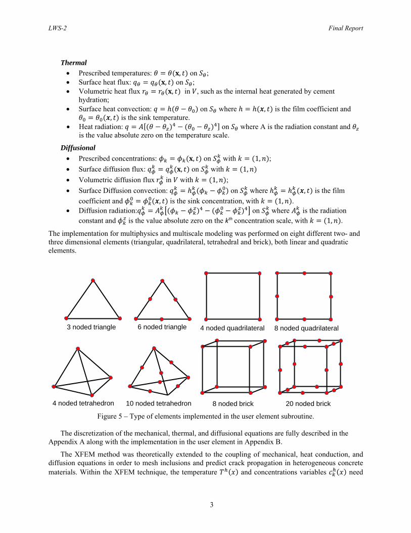
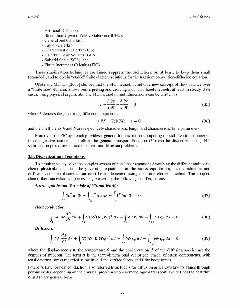
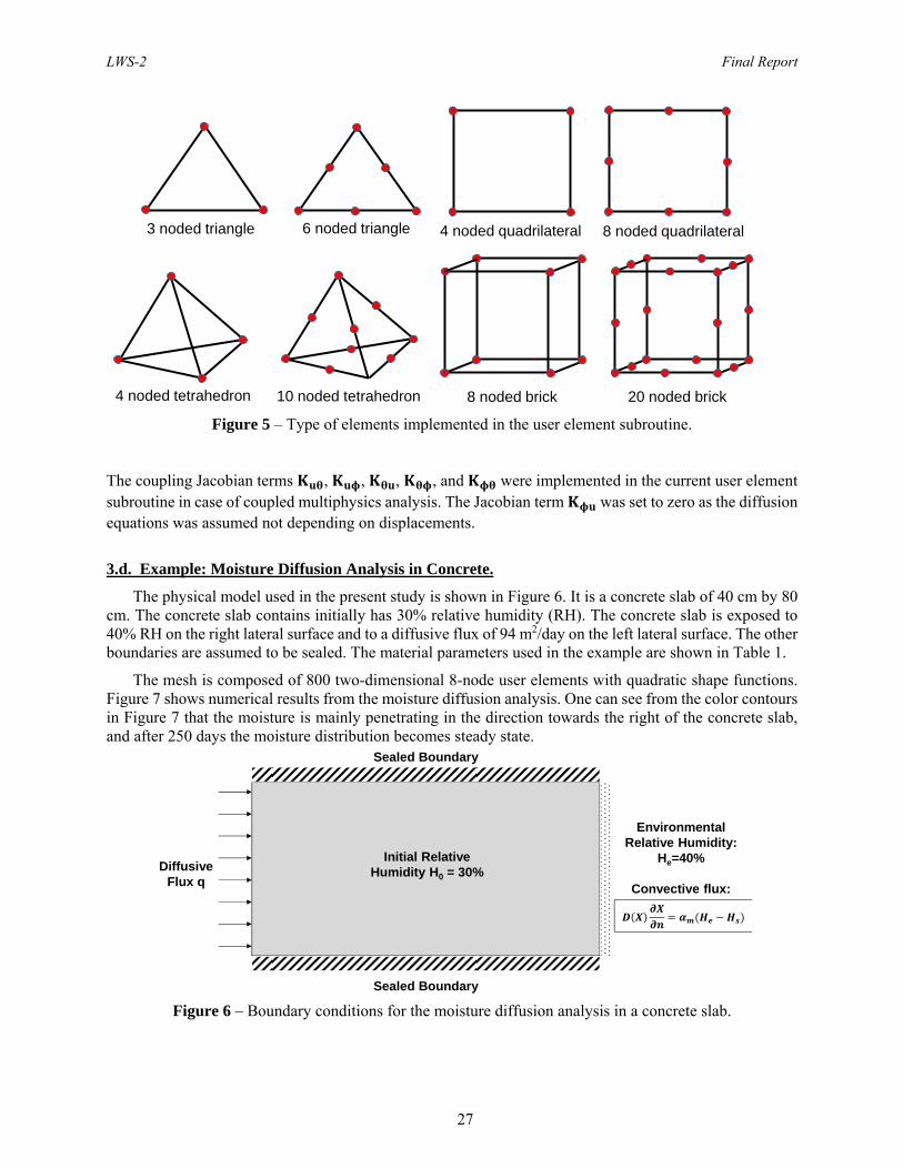
The implementation for multiphysics and multiscale modeling was performed on eight different two- and three dimensional elements (triangular, quadrilateral, tetrahedral and brick), both linear and quadratic elements.

Figure 5 – Type of elements implemented in the user element subroutine.

The discretization of the mechanical, thermal, and diffusional equations are fully described in the Appendix A along with the implementation in the user element in Appendix B.

The XFEM method was theoretically extended to the coupling of mechanical, heat conduction, and diffusion equations in order to mesh inclusions and predict crack propagation in heterogeneous concrete materials. Within the XFEM technique, the temperature and concentrations variables need

3 noded triangle 6 noded triangle 4 noded quadrilateral 8 noded quadrilateral

4 noded tetrahedron 10 noded tetrahedron 8 noded brick 20 noded brick

LWS-2 Final Report

4

also to be enriched with Heaviside and crack tip asymptotic functions, respectively and , in elements crossed by the crack path, as well as in blended elements (elements that are not crossed by crack paths but are composed of enriched nodes). The nodal enrichment is performed in a similar way to that of the displacement variables :

⋮ ⋮∈ ⋮∈ ⋮

∈

The durability model is based on the damage degradation of material properties of concrete. Using continuum damage mechanics (CDM), the damage is inserted in the model as an internal state variable (ISV) that deteriorates the mechanical properties of concrete. The damage evolution is characterized by the rate at which material damage is accumulated from the different degradation mechanisms that occurs at the microscopic level. The material damage in the concrete structure leads to the following degradation of material stiffness:

E E 1 D , 8

where is the material stiffness of the undamaged concrete structure. The damage variable is defined by assuming that the nuclear radiation can generate a specific damage process, , in addition to the mechanical, , and thermo-mechanical ones, :

D 1 1 1 1 9

To assess the aging degradation of concrete, a Multi-Stage Fatigue (MSF) model was used based on the deterioration of mechanical properties of concrete related to the total damage value. The microstructure-based MSF model incorporates different microstructural discontinuities effect (pores, inclusions, etc.) on physical damage progression. This model partitions the fatigue life into three stages based on the fatigue damage formation and propagation mechanisms:

- crack incubation (INC), - microstructurally small crack (MSC) and physically small crack (PSC) growth, and - long crack (LC) growth.

The total fatigue life is decomposed into the cumulative number of cycles spent in several consecutive stages as follows:

.

Finally, for the duration of this NEUP project, technology transfer to the NEUP sponsors was maintained through publication of technical reports. As deliverables, several files are provided with the final report::

Multiphysics Abaqus UEL user element subroutine Uel-Neup.f: a Fortran subroutine to solve multiphysics analysis for concrete structures (mechanical, thermal and diffusional). The subroutine internally calls a user material subroutine UMAT that can define the deterioration of mechanical properties.

Abaqus input files for 8 different user elements to be used in conjunction with the user element subroutine uel-neup.f;

LWS-2 Final Report

5

XFEM Abaqus UEL user element subroutine Uel-xfem.f: a Fortran subroutine to solve XFEM analysis [developed by Giner et al., 2009], which was translated from Spanish to English.

Abaqus input files for running a cracked finite strip loaded under uniform normal stress in conjunction with the user element subroutine uel-xfem.f;

Multi-Stage Fatigue Abaqus UVARM user subroutine Msf.f: a Fortran subroutine that evaluates the fatigue life of concrete at the end of each increment.

The multiphysics Abaqus UEL user element subroutine constitutes the main result of this work. This user element subroutine constitutes a multiscale and multiphysics platform in which several transport processes can be integrated by defining their material constants and solved simultaneously along with mechanical and thermal analysis. More advanced transport process models require a little further development in terms of implementation. This UEL subroutine is still limited to standard elements and is therefore unable to perform XFEM analysis in its current state. However, in the case of modeling strong and weak discontinuities within concrete structures, the XFEM theory requires a partitioning of the cut elements into subelements for integration purposes. Therefore, the current user element implementation can be called for each of these subelements, and by incorporating additional enrichment functions to the current approximation, the extension to the XFEM capability is straightforward.

LWS-2 Final Report

6

Table of Contents

1. Introduction ………………………………...………………………………………………….……7

2. Mass Transport Processes in Concrete …..…………………………………………………………11

2.a. Concrete Material Overview ………………………………………………………….…11

2.b. The Hydration Process: CSH Formation Reaction ………………………...…………….15

2.c. Phenomena at work…..16

3. Multiphysics and Multiscale Modeling………………………………………………………...…..20

3.a. General formulation of the transport equality ………………….………………………..20

3.b. Discretization of equations …………………………………………...…………………23

3.c. Implementation in the user element subroutine UEL ……………………………………25

2.d. Example: Moisture Diffusion Analysis in Concrete …………………………………….27

4. Extension of the UEL development to the XFEM ………………………………………………….29

5. Aging Degradation of concrete ...…………………………………………………………………..37

5.a. Damage modeling ……………………………………………...………………………..38

5.b. Fatigue modeling ……………………………………….…………...…………………..40

6. Conclusions …………...………………………………………………………………….………..41

References ……………………………………………………………………………………...……..41

Appendix A – Discretization of governing equations and implementation in UEL subroutine …...…45

Appendix B – Implementation in UEL Subroutine ……………………………………………………55

LWS-2 Final Report

7

1. Introduction

Extensive research and studies have been carried out to determine the durability of concrete and quantify the effects of age-related degradation on the performance of nuclear power plant (NPP) safety-related structures under various service conditions [Naus, 2007, 2009; Maekawa et al., 2003, 2009]. Thus, the background information and data on the progressive changes in the physical and chemical nature of concrete under the exposure of the environment (i.e., elevated temperature, moisture, corrosion, irradiation, cyclic loadings, etc.) is available and very detailed in the literature [Maekawa, 2009; Naus, 2009; Bejaoui, 2007, Gawin et al., 2006; Fillmore, 2004]. The existing studies describe the mutual linkage of chemo-physics and mechanistic events which develop over the representative volume element (RVE) of different scales and, are used to simulate the macroscopic behaviors of structural concrete under combined external loads and ambient conditions.

There are currently 99 nuclear power plants (NPPs) in the United States, collectively which provided approximately 20% of the nation’s electricity [Naus et al., 2008]. The low cost, mechanical properties, and high water content of reinforced concrete make it a suitable building material for use in a variety of structures found in NPPs, most notably in the construction of reactor containment units. As many of the terms of licensure for operation of these NPPs must soon be renewed, the conditional assessment of the concrete structures within is increasingly important. However, many current experimental techniques used in the conditional assessment of concrete are either insufficient with regards to their ability to provide predictive information with respect to service life, or are destructive in nature, and therefore of limited utility. Taking this into account, the development of an integrated computational modeling scheme for use in predicting the long term behavior of reinforced concrete is seen as highly desirable.

In the past decades, considerable research and modeling efforts have been put into the improvement of the durability of concrete structures by developed countries, such as United States, Canada, Japan, and several European countries. This has resulted in a characterization and reasonable understanding of the main degradation processes, and an acquired experience in establishing measures to prevent these degradation processes. The results of these efforts can be found in the present literature, concrete codes and manuals on durability design. Many fundamental efforts that have been published on modeling aging degradation and assessing the effect of deterioration mechanisms of the performance of nuclear safety-related concrete structures under the exposure to the environment (e.g., temperature, moisture, radiation, cyclic loadings, etc.). The synthesis of these investigations on concrete and reinforcement degradation and general guidelines for probabilistic durability design were published in the literature. Several models and software codes that were developed to predict the durability of concrete structures have been developed for evaluating aging degradation of concretes. Some of the software codes and their descriptions are listed as follows:

DuCOM (the acronym for Durability of COncrete Model): It is a Finite-Element-based computational program which has been developed in the concrete laboratory at the University of Tokyo since 1990 to evaluate various durability aspects of concrete [Maekawa et al., 1999]. The current full version traces the development of concrete hardening (hydration), pore structure formation, transport and equilibrium of vapor and liquid condensed water in the pores, and several associated nonlinear mechanical behaviors, such as autogenous/drying shrinkage, stress generation, and cracking, from casting of concrete for a period of several months or even years. The program can be utilized to study the effect of ingredient materials and environmental conditions, as well as the size and shape of the structure on the durability of concrete; it can be used to analytically trace the evolution of the microstructure, strength and temperature in time for arbitrary initial and boundary conditions [Maekawa et al., 2003, 2009]. DuraCrete (European durability concept of concrete): In this Brite-EuRam project, the durability design has been developed into a service life design based on performances and on reliability for reinforced concrete structures. The software offers the possibility to present the design on the same level as the structural design that has also been based on performances and reliability. The structural and service life

LWS-2 Final Report

8

design can even be integrated. The "DuraCrete" approach offers good opportunities for the service life design of other structural materials and building materials. Life-365 is a computer program for predicting the service life and life-cycle costs of reinforced concrete exposed to chlorides. It follows a methodology created by the American Concrete Institute (ACI) strategic development council consortsium I and II groups of companies that gives research-based estimates of the effects of concrete design, chloride exposure, environmental temperature, concrete mixes and barriers, and steel types on this service life and life-cycle cost. DuraNET: Network for supporting the development and application of performance based durability design and assessment of concrete structures. It is an international engineering professional network which aims to promote the adoption and wider use of a performance and reliability based service life design approach for reinforced concrete structures. This European Union funded network brings together 19 partners from across Europe who are committed to improving the durability design, assessment and repair of concrete structures in Europe. The network aims to promote the use of service life design of concrete structures based on a probabilistic design method. Hypercon: Prediction and Optimization of Concrete Performance research program from BFRL (Building and Fire Research Laboratory, NIST) to develop and implement the enabling measurement science that gives the concrete industry and state and federal government agencies the predictive capability upon which they can base the use of performance-based standards and specifications in key technical areas [Snyder and Bentz, 2009]. The Hypercon program offers freely available software to the general public such as CIKS (Computer Integrated Knowledge System for High Performance Concrete that addresses the service life prediction of steel-reinforced concrete exposed to chloride ions), CEMHYD3D (3D cement hydration and microstructure development modeling package), HCSSMODEL (3D concrete microstructure modeling package, etc.

The use of concrete in nuclear facilities for containment and shielding of radiation and radioactive materials has made its performance crucial for the safe operation of the facility. This concrete is exposed to several conditions that have been shown to cause the concrete to deteriorate. These conditions include: freeze/thaw, heat, cracking, acids, chlorides, sulfates, carbonation, calcium leaching, and radiation. These conditions are compounded by the aging of these concrete structures [Fillmore, 2004]. It is therefore primordial to accurately characterize and model the mechanisms responsible for degradation of reinforced concrete structures to obtain a good prediction of the durability of reinforced concrete structures.

A numerical multiscale modeling scheme similar to that of Maekawa et al. [2003, 2009] shown on Figure 1, should include a frame of structural mechanics that has an inter-link with thermo-hydro physics in terms of mechanical performances of materials through the constitutive modeling in both space and time, and described as following:

Cement heat hydration and thermal conduction: The reaction of water with cement is exothermic and generates a considerable amount of heat over an extended period of time. Water content, density, and temperature significantly influence the thermal conductivity of a specific concrete. Pore structure formation model of cement paste: Computational modeling of varying micro-pore structures of hardening cement paste media is a central issue of multiscale analysis. Moisture migration and durability related substances (in this study, calcium, chloride, dissolved CO2 and O2 are treated) and diffusion of gaseous phases are greatly governed by micro-pore structures. Moisture equilibrium and transport (including frost): Moisture mass balance must be strictly solved in both vapor and condensed water. The conservation equation is expressed with capacity, conductivity and sink terms on the referential volume. Pore pressure of condensed water is selected as a chief variable so that both saturated and unsaturated states can be covered with perfect consistency. Another key issue here is that material characteristic parameters are variable with respect to micro-pore development. Free/bound chloride equilibrium and chloride ion transport: Chloride transport in cementitious materials under usual conditions is an advective-diffusive phenomenon. In modeling, the advective

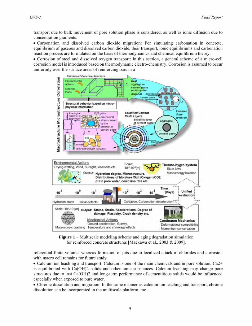
LWS-2 Final Report

9

transport due to bulk movement of pore solution phase is considered, as well as ionic diffusion due to concentration gradients. Carbonation and dissolved carbon dioxide migration: For simulating carbonation in concrete, equilibrium of gaseous and dissolved carbon dioxide, their transport, ionic equilibriums and carbonation reaction process are formulated on the basis of thermodynamics and chemical equilibrium theory. Corrosion of steel and dissolved oxygen transport: In this section, a general scheme of a micro-cell corrosion model is introduced based on thermodynamic electro-chemistry. Corrosion is assumed to occur uniformly over the surface areas of reinforcing bars in a

Figure 1 – Multiscale modeling scheme and aging degradation simulation

for reinforced concrete structures [Maekawa et al., 2003 & 2009].

referential finite volume, whereas formation of pits due to localized attack of chlorides and corrosion with macro cell remains for future study. Calcium ion leaching and transport: Calcium is one of the main chemicals and in pore solution, Ca2+ is equilibrated with Ca(OH)2 solids and other ionic substances. Calcium leaching may change pore structures due to lost Ca(OH)2 and long-term performance of cementitious solids would be influenced especially when exposed to pure water. Chrome dissolution and migration: In the same manner as calcium ion leaching and transport, chrome dissolution can be incorporated in the multiscale platform, too.

LWS-2 Final Report

10

Macro-damage and crack evolution and momentum conservation: For simulating structural behaviors expressed by displacement, deformation, stresses and macro-defects of materials in view of continuum plasticity, fracturing and cracking, well established continuum mechanics are available in the multiscale modeling theory. Compatibility condition, equilibrium and constitutive modeling of material mechanics are the basis and spatial averaging of overall defects in control volume of mesoscale finite element is incorporated into the constitutive model of quasi continuum. In a 3D finite element computer code of nonlinear structural dynamics, the size of a referential volume is in the order of 10-3~10-1m. Creep and cyclic loading: Two important aspects of durability of fastening elements in concrete and reinforced structures are the effect of repeated loading and the interaction between concrete cracking and deformation that occurs while concrete is under sustained stress (creep of concrete). Cyclic variations of environmental relative humidity have an appreciable effect on the long time deformations of concrete structures.

The events listed above are not independent but mutually interlinked with each other. A complex figure of interaction can mathematically be expressed in terms of state parameters commonly shared by each event. For example, Kelvin temperature and pore water pressure can be seen in the modeling of cement hydration rate, moisture equilibrium, constitutive law of hardened cement paste, conductivity of carbon dioxide, bound and free chloride equilibrium, etc. Each of these mechanisms are individually modeled with different geometrical scales of representative volume element (RVE) within a used-defined material subroutine.

Various damage mechanisms and durability issues lead to very complex fracture behavior inside heterogeneous materials, such as concrete. Therefore, the prediction of crack propagation and fracture resistance can help design durable concrete materials to avoid the excessive damage [Ng and Dai, 2011]. Concrete materials are characterized by random, complex and heterogeneous microstructures, which include the very irregular aggregates, matrix, air voids, and interfacial adhesion zones. The crack evolutions are affected largely by their detailed microstructures. In the past, several numerical approaches have been developed to predict the crack propagation in such materials. Among these numerical approaches, cohesive zone modeling has been of the most used fracture modeling over the past decades. However, this fracture modeling techniques, like other conventional finite element based methods, requires that the mesh conforms to the geometric discontinuities. The only possibility to accurately model these geometric discontinuities is to conform the finite element mesh to the line of discontinuity. The eXtended Finite Element Method (XFEM), initially proposed by Belytschko and Black [1999] and Moës et al. [1999], has been developed to arbitrarily handle strong (cracks) and weak discontinuities (material interfaces). XFEM is based on the local extrinsic partition of unity enrichment which was initially used to model strong discontinuities, i.e. cracks, in meshless methods [Rabczuk and Wall, 2006].

Numerical analyses of structures made of quasi-brittle materials, such as concrete, require robust models for the opening and propagation of cracks, which represent the discontinuous character of the fracture process and adequately consider cohesive forces acting within the fracture process zone. During the last decade, approaches that allow for the representation of cracks as embedded discontinuities within the structure independent of its discretization have been developed. These formulations can be categorized into element-based formulations, generally denoted Embedded Crack Models and nodal-based formulations, such as the Extended Finite Element Method (XFEM). Cracking in quasi-brittle materials, such as concrete, is characterized by the formation of microcracks which eventually coalesce and form propagating macrocracks. The realistic modeling of these processes of crack opening and propagation is a prerequisite for reliable prognoses of the safety and the durability of reinforced concrete structures. In these approaches, the correct prediction of the direction of new crack segments is crucial for the reliability, as well as for the robustness of the numerical analysis.

Therefore, it is primordial to accurately and efficiently develop robust multiscale continuum damage models of mechanisms that capture the degradation at different length scales and their mutual effects on

LWS-2 Final Report

11

initiation and propagation of microcracks and macrocracks, in order to establish a direct relationship with the durability of concrete structures of NPP.

This report describes the development a modeling platform to solve multiscale and multiphysics equations for aging degradation of concrete structures in nuclear power plants (NPP) and to validate the models with experimental data from the literature. Numerical solution procedures for coupled chemo-mechanical simulations of concrete structures subjected to aggressive substances and mechanical damage are presented within user elements and into a finite element code.

2. Mass Transport Processes in Concrete 2.a. Concrete: Material Overview

Concrete has a long and well documented history of use. In spite of this, a comprehensive understanding of all of the processes at work in concrete, especially steel reinforced concrete remains has remained elusive until recently. The recent characterization of chemical and mechanical properties of the cement binder of commonly used Portland cement was provided in the works of Bonaccorsi et al. [2005], Richardson [2008] as well as Pellenq et al.[2008], has provided a means by which cement, and therefore concrete, may be understood at micro- and nano-scales. This, when combined with the techniques and methods of quantum, continuum, fluid, and fracture mechanics, and thermodynamics provide a means by which one may simulate the combined processes at work within the “living” material of concrete. While it is true that simulations have been used in the past to provide some insight into these processes, particularly heat, moisture, and chemical movement within a concrete system, most of these simulations have been limited in their scope to describing only one or a few of these processes at a time. In a material such as concrete, whose chemical composition and mechanical properties are ever changing and tightly coupled, this can hardly be considered adequate. This taken into consideration alongside the fact that, many times, current service life assessment techniques are either destructive or limited in their applicability, the need for simulations capable of describing all of the complex interactions taking place within a concrete structure becomes apparent. To this end, what follows is a brief description of the theory behind these processes. Macro/Continuum Scale At the continuum scale we are able to identify the various phases that make up reinforced concrete in its entirety. The solid phase aggregate, cement binder, and steel reinforcement are easily identified by casual inspection. However, less immediately obvious is the liquid and gaseous phases contained within the pore matrix of the cement binder. Furthermore, depending upon the age and exposure to aggressive chemical species like CO2 and various chlorides, additional solid phases must be considered as cement binder is carbonated and general corrosion oxide buildup accrues on the interfacial area between the binder and reinforcement. At this length scale, the use of continuum mechanics in treating stresses, quantity of energy, entropy, and quantity of the various phases as scalar, vector, or tensor quantities is prevalent in numerous concrete behavior models. This allows for the use of differential and integral calculus in describing said behavior, and in doing so gives one access to the methods and balance laws of continuum mechanics. As we are concerned with the transport of mass and energy within the given concrete system, we are particularly interested in the balance laws corresponding to these phenomena, of which the general form for a given quantity of interest A is as follows:

∙ 0. 1

On the domain of interest, is the scalar potential function for A at a given point, is the vector function describing convective flow across an infinitesimally small surface of the domain of A, is the scalar density function of A, is the scalar concentration function of A, is the scalar sink function for a given point [Kuzmin, 2010]. In the case of entropy balance, we change the state of equality, “=”, to one of inequality,

LWS-2 Final Report

12

“ ”, as is consistent with the Clausius-Duhem inequality. The general form beyond this small but important consideration, however, remains unchanged. Additionally, in order to couple transport processes with mechanical deformations, we must also consider the use of the balance laws of momentum, be they linear or angular, in accordance with the specific geometry of the domain. These balance laws, while powerful, are useful only if we have enough constitutive equations to properly constrain the resulting system of equations. Each concrete model has its own set of constitutive equations, many of which depend upon the characteristics of the concrete structure at a sub-continuum level. For this section, though, it must be noted that accurate simulations of reinforced concrete as a whole are predicated on a comprehensive treatment of each phase not only in a vacuum, but also in the context of their combination. However, the complexity and somewhat random distribution of some of these phases throughout the reinforced concrete body, in particular, the aggregate and the fluid content of the pore structure, make the specific treatment of each instance of these phases difficult if not impossible at the continuum length scale alone. Additionally, many models used to describe transport phenomena in concrete at the continuum level were of a general form for use in a variety of porous media in building and soil physics. As Cerny and Ravnanikova [2002] point out, many of these models were adapted by the inclusion of sink/source terms in the general transport PDE for use in concrete modeling. As a consequence, until recently, this has resulted in a number of models that were limited in their applicability due to having been developed without fully considering the effects of both the pore structure and the inclusion of aggregates on the thermodynamic, mechanical, and chemical processes of reinforced concrete. Furthermore, a number of these models failed to address the synergistic effects of coupling multiple transport phenomena. For instance, the Fickian diffusion based models for chloride transport in concrete of Tuutti [1982], Funahashi [1990], Cady and Weyers [1992], Zemajtis et al. [1998], and Costa and Appleton [1999] all neglected the affect that moisture transport would have on the ingress of chlorides [Cerny and Ravnanikova, 2002]. Even when the effects of coupling multiple phenomena were explored, as in the work of Majorana et al. [1998], which was itself based off of the works of Bazant and Najjar [1972], and Bazant and Thonguthai [1979], the effects of aggregates were still not included in the model.

In order to account for the effects of aggregates, a number of approaches in modeling the material behavior of the aggregates, steel, and voids suspended in the cement matrix at lower length scales have been and are being taken, with results being “fed upwards” into coefficients included in the system of coupled PDEs at the continuum level. In effect, this smears or averages out the thermodynamic, mechanical, and chemical properties of the phases across the material continuum, thereby addressing the discontinuities inherent in their inclusion. A notable example of this kind of approach is found in Maekawa’s [2009] multi-scale model of concrete, in which the idealized pore volume and pore surface area are modeled as statistically stored variables across a given representative volume element (RVE) at lower length scales, and whose thermal, chemical, and mechanical behavior is averaged across said element. A more recent trend has been to try and capture the geometry of a concrete RVE containing aggregates, voids, and pores with discretization methods like Asahina and Bolander’s Voronoi tessellation [2011], Rashid’s use of the polyhedral element method (PEM) [Rashid and Sadri, 2012], and, of course, the employment of extended finite element method (XFEM) by various authors. The use of these techniques is further detailed in the following section dealing with the mesoscale characteristics of reinforced concrete. Mesoscale Of particular importance in simulating the movement of both chemical species and energy within a reinforced concrete system is the quantification of its porous nature. This quantification also aids in helping to simulate the behavior of crack propagation within the very same system. The complex capillary pore network encountered at the mesoscale contains pores that typically have a radius in the range of magnitude of 10-6m to 10-3m. Many models seek to characterize the porous nature of concrete at this scale by developing a pore distribution curve, f(r), which when integrated over the domain of all possible pore radii,

to , yields the following equation:

LWS-2 Final Report

13

1. 2

This pore distribution is used in the definition of permeability, K, and hydraulic conductivity, k, which are defined as

18

3

and

8 4

respectively. In this, is the effect of tortuosity, and exists on the interval 0< < 1. is the density of the fluid being conducted, g represents the acceleration of the fluid due to gravity, and is the dynamic viscosity of the same fluid. Moisture content by volume across a given domain of radii may be found by multiplying the integral across said domain by the saturated moisture content of the system,

5

Lastly, we may use the distribution function to calculate the relative moisture diffusivity as follows:

. 6

It is important to realize that in looking for , , we are holding equal to . This implies that w is equal to and, therefore, becomes a constant. Since this cannot happen in theory, the moisture gradient cannot be chosen as the driving force of the transport process. For this, a different thermodynamic force must be selected, as was the case when Maekawa et al. [2009] selected the pressure gradient. By assuming that pore formation does not take place in the hydration of the inner core of a reacting grain and that the porosity at position x in a CSH grain varied linearly with the radius, Maekawa et al. [2009] was able to define a relation between position and porosity of the form

7

where is the porosity, and D is the size of a given CSH grain. Multiplying this term by the appropriate area dimensions and integrating over the domain of the system yields the total volume within the concrete body occupied by pore space:

4 . 8

This value may then be used to calculate the void volume fraction of a representative volume element at this scale. This value contributes in the simulation of crack propagation in the cement matrix. It is important to note that all of these relations are effectively smearing the behavior of the complex geometry of the pore structure across an RVE. Furthermore, none of them reference the inclusion of aggregates in the calculations. Recently, many have sought to simulate the effect that such inclusions would have on the behavior of concrete through the use of numerical techniques similar to Finite Element Method (FEM). Rashid and Sadri [2012] make use of Polyhedral Element Method (PEM) to discretize the geometry of the RVE. PEM, though perhaps more computationally demanding depending on the problem size, may be viewed as preferable to standard FEM in that it produces a significantly smaller error in meshing concave

LWS-2 Final Report

14

geometries. This is possible because the each element in the mesh is further divided into sub-cells, and the shape function defined across the entire element is defined only at specific points within these cells. In this way, PEM is not dependent on the continuity of the whole element. Asahina and Bolander [2011] were able to use Voronoi-based discretization to represent multiple particles of complex geometries suspended in a matrix. Micro-scale During the process of hydration, contacting water and grains of calcium silicates like alite (C3S) and belite (C2S) react to form calcium silicate hydrates (CSH). At higher length scales, the CSH appears amorphous to the point where it is often referred to as a gel. Closer inspection on the length scale of up to 500nm reveals CSH to be somewhat structured. While hydration that takes place on the interior of a hydrating grain may indeed be considered amorphous, the hydration that takes place on the surface of said grain exhibits a more regular structure (Figure 2).

Figure 2 – TEM micrograph showing the inner and outer products of hydrating C3S. Note the contrast

between the amorphous inner product and the semi-ordered outer product [Pellenq et al., 2008].

As hydration occurs on the surface, CSH particles that form from the reaction between silicates dissolved into the reacting water begin to flocculate, and deposited on the surface of aggregates, and other, larger hydrating CSH grains. These particles are composed of stacks of tens to hundreds of CSH lamella, the specific dimensions of which are functions of Ca:S ratio of the mixture and the amount space in which these lamella have to grow. The lamella do not grow indefinitely though, as they exhibit a tendency towards disorder at long range. The orientations of the lamella are far from uniform, thereby accounting for the apparent isotropy at longer ranges. Pellenq et al. [2008] were able to determine using ab initio calculations, energy minimization techniques, and molecular dynamics to show that CSH is essentially a lacunar ion-covalent continuum at

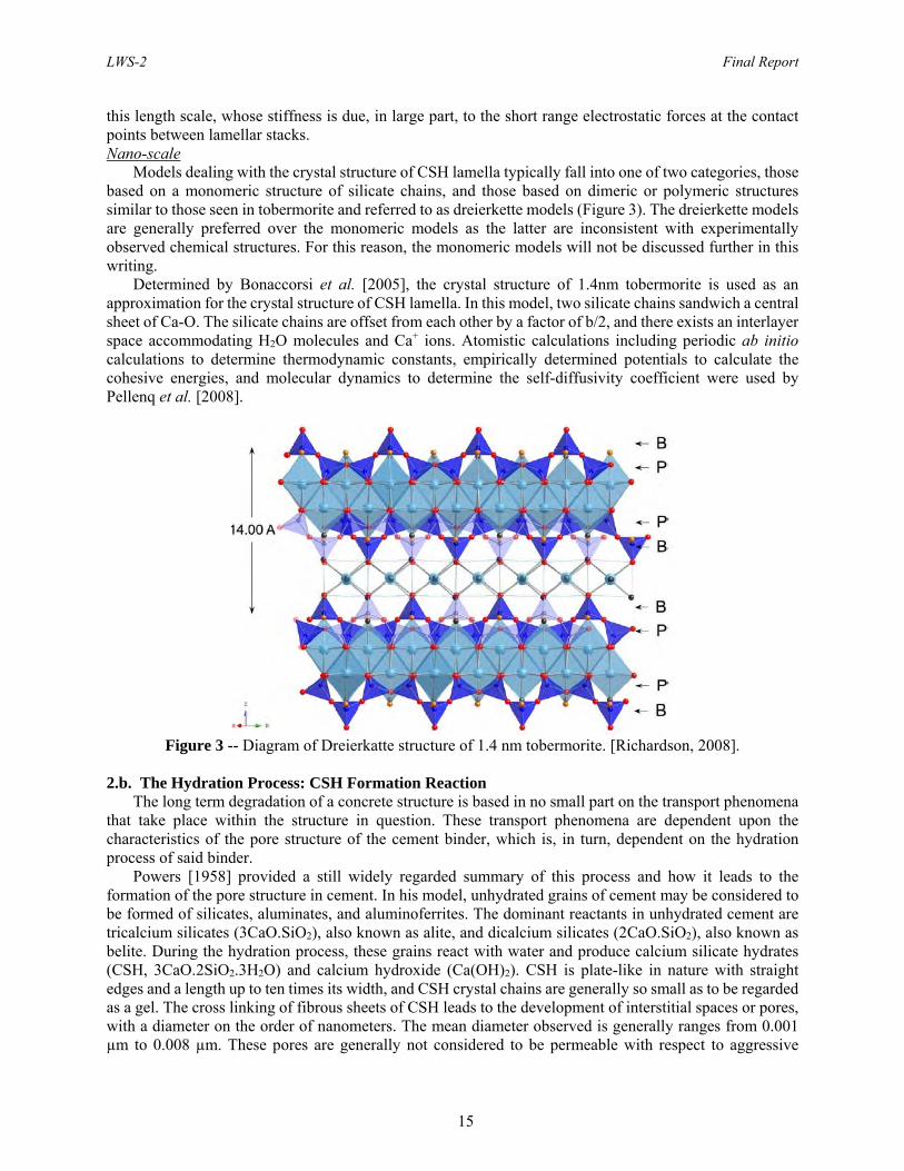
LWS-2 Final Report

15

this length scale, whose stiffness is due, in large part, to the short range electrostatic forces at the contact points between lamellar stacks. Nano-scale Models dealing with the crystal structure of CSH lamella typically fall into one of two categories, those based on a monomeric structure of silicate chains, and those based on dimeric or polymeric structures similar to those seen in tobermorite and referred to as dreierkette models (Figure 3). The dreierkette models are generally preferred over the monomeric models as the latter are inconsistent with experimentally observed chemical structures. For this reason, the monomeric models will not be discussed further in this writing. Determined by Bonaccorsi et al. [2005], the crystal structure of 1.4nm tobermorite is used as an approximation for the crystal structure of CSH lamella. In this model, two silicate chains sandwich a central sheet of Ca-O. The silicate chains are offset from each other by a factor of b/2, and there exists an interlayer space accommodating H2O molecules and Ca+ ions. Atomistic calculations including periodic ab initio calculations to determine thermodynamic constants, empirically determined potentials to calculate the cohesive energies, and molecular dynamics to determine the self-diffusivity coefficient were used by Pellenq et al. [2008].

Figure 3 -- Diagram of Dreierkatte structure of 1.4 nm tobermorite. [Richardson, 2008].

2.b. The Hydration Process: CSH Formation Reaction

The long term degradation of a concrete structure is based in no small part on the transport phenomena that take place within the structure in question. These transport phenomena are dependent upon the characteristics of the pore structure of the cement binder, which is, in turn, dependent on the hydration process of said binder.

Powers [1958] provided a still widely regarded summary of this process and how it leads to the formation of the pore structure in cement. In his model, unhydrated grains of cement may be considered to be formed of silicates, aluminates, and aluminoferrites. The dominant reactants in unhydrated cement are tricalcium silicates (3CaO.SiO2), also known as alite, and dicalcium silicates (2CaO.SiO2), also known as belite. During the hydration process, these grains react with water and produce calcium silicate hydrates (CSH, 3CaO.2SiO2.3H2O) and calcium hydroxide (Ca(OH)2). CSH is plate-like in nature with straight edges and a length up to ten times its width, and CSH crystal chains are generally so small as to be regarded as a gel. The cross linking of fibrous sheets of CSH leads to the development of interstitial spaces or pores, with a diameter on the order of nanometers. The mean diameter observed is generally ranges from 0.001 µm to 0.008 µm. These pores are generally not considered to be permeable with respect to aggressive

LWS-2 Final Report

16

species. They are known as gel pores or micro pores. They occupy approximately 1/3 of the volume of the gel volume. Calcium hydroxide is more crystalline in structure.

As the unhydrated silicates react with the water, the CSH grains grow, interlock, and bond both physically and chemically. It is this process that gives concrete its structural properties, since larger pores form at the boundaries of the CSH grains/clusters. These pores are known as capillary pores. They may be thought of as the voids left by water that has either reacted chemically with the unhydrated cement, or evaporated during the course of the reaction. Capillary pores are considerably larger than gel pores, though their precise dimensions are affected by water to cement ratio and the level of compaction in the hydrating mixture.

Additionally, pockets of air may become trapped inside the gel during hydration, even though most of these pockets should be removed during the process of compaction. There are also voids left in the concrete by the aggregate, though, due either to compaction surrounding the aggregate or the impermeable nature of the aggregate itself, these voids do not generally contribute to permeability.

Maekawa et al. [2009] take advantage of the fact that hydration is an exothermic process, and are able to characterize it based on this. In this model, the rate of hydration is taken to be a function of water to cement ratio, the accumulated heat of the hydrating body, and the chemical composition of the cement allowing for the inclusion of additives like fly ash, blast furnace slag, superplasticizers, and pozzolans. Maekawa also includes the presence of gypsum as a reactant in the makeup of unhydrated cement. This leads to an intermediate stage in the process where the aluminate and ferrite phases react with the gypsum to produce gypsum, which retards the hydration process until it is converted by newly formed calcium aluminate hydrates into monosulphates.

All of these reactions occur simultaneously, though the reaction rates of each reactant are different. Over the course of the hydration process, the heat generation profile of different reactants comes to dominate the overall heat generation profile of the whole process as those constituents with faster rates of reactions exhaust themselves and slower reacting constituents take their place as the principle source of hydration. Thus, Maekawa et al. [2009] observed the overall level of hydration by noting the rate of heat generation of the body in question. This may be computed as the sum of the heat generation rates of the constituent parts of the cement mixture

. 9

Where Hc is the total heat rate for the cement compound, pi is the weight composition ratio for the ith component, and Hi is the heat generation rate for the ith component.

Other hydration models exist, and they may largely be categorized as one of four different types. These are Overall Kinetics – Hydration is described as a function of time. No explicit consideration is given to

mechanisms and processes at particle level. Particle Kinetics – Reactions at particle level are taken as the starting point. There is no interaction

between particles, however. Hybrid Kinetics – Particle size, distribution, and other factors (water/cement ratio, chemical

composition, etc.) are considered explicitly. Integrated Kinetics – The hydration process is considered as part of an overall model for development

of material properties (example: DuCOM).

2.c. Phenomena at Work In assessing the performance of steel reinforced concrete, a host of phenomena can be observed at work in a manner which may adversely affect the service life of a given structure. Additionally, the deleterious effects of many of these phenomena may have synergistic relationships, and so, must be considered in concert for the sake of accuracy of prediction. For the purposes of this work, these phenomena considered are as follows.

LWS-2 Final Report

17

Corrosion of Steel Reinforcement The corrosion of steel reinforcement is the primary factor in the degradation of structural performance

in reinforced concrete [Richardson, 2002]. In distributed corrosion, the buildup of corrosion product causes a separation of the binder from the reinforcement and will result in cracking or spalling. Localized corrosion results in a loss of strength of the steel reinforcement due to a loss in cross sectional area of the steel. In either case, the detection of either form by non-destructive means is problematic.

In reinforced concrete, corrosion is an electrochemical process in which the steel reinforcement reacts with oxygen and moisture found in both the contents of the pore structure and cement binder itself. As such, the advancement of this process is typically couple with both oxygen and moisture transport throughout the concrete structure. The steel found in fresh concrete is typically surrounded by a passive film that inhibits the corrosive process. The protective quality of this film is reduced in the presence of critical levels of chlorides within the surrounding volume, and the film itself is directly attacked by the carbonation reaction brought on by the ingress of CO2. As such, the transport of both of these quantities must be taken into consideration when trying to accurately predict the rate of corrosion as well.

Corrosion occurs when the cement binder surrounding the steel reinforcement becomes sufficiently saturated by moisture and oxygen to enable it to begin acting as an electrochemical cell. Once this has occurred, if the protective layer surrounding the steel reinforcement is depassivated or penetrated, a local anode forms in the reinforcement. At this point, the iron, Fe, in the steel is oxidized, transferring its electrons to and reducing the positively charged hydroxyl, OH+, ions at the cathode. The actual location of the cathode relative to the anode within the structure may vary. In some cases, a decidedly local depassivation of the protective layer surrounding the reinforcement can result in the cathode forming within the same steel body, and is characteristic of pitting corrosion. In other cases, the site of the cathode may be in another nearby steel body contained within the cement matrix, or even, in the case of the formation of a macro-cell, another section of the structure’s geometry entirely. The relative positions and sizes of the anode and cathode within the electrochemical cell may have pronounced effects on the rate of corrosion.

Regardless of the type of corrosion present in the steel reinforcement, given a certain level of moisture saturation and depassivation of the protective layer, the rate of corrosion is limited by the rate of flow of electrons between the anode and cathode so long as there is no outside source of new electrons. This electron flow rate may be defined to be the number of electrons flowing per unit area and is referred to as the corrosion current density. Faraday’s laws may be used to describe the relationship between the corrosion current density and amount of mass lost to corrosion in a given system. From Faraday’s Second Law of Electrolysis, that is, that the mass of different substances liberated given a quantity of electrical charge is proportional to the ratio of the atomic mass and the valence, yields

10

where is the mass lost, is the atomic mass of the ions in question, is the electric charge, is the valence, and F is Faraday’s constant. Rodriguez et al. [1996] was able to describe the depth of penetration of pitting corrosion using Faraday’s Laws with following system of equations:

11

and

0.115 12

where is the residual bar diameter, is the initial bar diameter, takes the value of 2 or 8 in the cases of general and pitting corrosion respectively, is the depth of penetration into the reinforcement, is the corrosion rate, and t is the time since the onset of corrosion measured in years.

LWS-2 Final Report

18

Moisture Transport Water is a primary reactant in many of the chemical reactions that takes place in reinforced concrete, a common solvent for many of the aggressive species at work in reinforced concrete, acts as a means of energy conveyance (as in the case of heat), and is also a source of mechanical stresses due to freeze/thaw processes in the pore structure of concrete. It is for these reasons that accurate simulation of moisture transport is of paramount importance when making service life predictions for reinforced concrete structures. The movement of moisture in a body of concrete has been described in a number of ways. As concrete is a porous medium, the ingress of fluid moisture may be described in terms of pressure differential driven capillary action by the following relationships

√ 13

14

√ 15

where is the cumulative volume of absorbed liquid, is the cross-sectional area exposed to the liquid, is the sorptivity, is time, is the cumulative liquid intake and is the porosity. Moisture in the form of vapor may travel through concrete by means of gaseous diffusion, as described by Fick’s first law of diffusion as described by the following equation

16

where is the mass transport rate in terms of mass per area per second, is the diffusivity coefficient, c is the moisture concentration, and x is position. Ionic diffusion, described by Fick’s second law, may also be used to describe the flux of moisture, particularly during the diffusion controlled stage of hydration, wherein moisture transport into the center of hydrating CHS grains is dominated by this process. As with gaseous diffusion, it is typically driven by differences in concentration. It is given by the general form:

17

One difficulty in inherent in the use of Fick’s first and second laws of diffusion in describing transport lies in characterizing the diffusion coefficient, . In concrete we cannot assume perfect continuity of the cement binder, and so, the porosity and tortuosity of the system must be taken into account. Maekawa et al. [2009] defined these terms as scalar coefficients contained within D itself, and in both cases, calculated their value based on smeared or averaged characteristics found at lower length scales. Furthermore we cannot assume D is a constant scalar. In defining D to be a scalar field, we introduce a nonlinearity that necessarily changes the general form of Fick’s second law to:

∂∂x

∂∂x

18

as was the case when this form of the diffusion equation was derived by Klute [1952]. Lastly, depending on the physical characteristics of the concrete body in question, it may be necessary

to describe moisture transport in terms of convective motion. General convection may be described by the Richards equation as:

∙ 19

where is the hydraulic conductivity or filtration coefficient, H is the pressure head, and h is the total head.

LWS-2 Final Report

19

In the general form of the transport PDE, the total flux of a given quantity is typically decomposed into diffusive and convective terms, which take the form of the two previous methods of transport. In many systems, it becomes necessary to consider the total moisture content at a given point as being the sum of moisture found in both liquid and gaseous phases, as is the case in Maekawa et al. [2009]. Oxygen Transport As the corrosion process of steel reinforcement in concrete structures is limited by the availability of oxygen at the cathode site, oxygen movement and content within said structures must be considered. The total ingress of oxygen in a concrete system may be described both in terms of a gaseous phase in addition to oxygen dissolved in liquid moisture. As such, oxygen transport is at least partially coupled with moisture transport, specifically of the liquid phase. The processes by which oxygen is transported within a concrete system are gaseous and ionic diffusion, and convective transport as detailed in the previous section. Chloride Ion Transport Free chlorides introduced into a concrete structure will, if allowed to attain a certain concentration threshold in the area of the steel reinforcement, accelerate the corrosion process. The exact process by which this occurs is not entirely understood. This may be due to the chlorides reacting either with the passive layer surrounding the reinforcement, or this may be due to the preferential reaction of the chlorides with iron ions. In any case, what is agreed on is the notion that chloride transport is dominated by Fickian diffusion and capillary action, as free chlorides are introduced primarily in solution with moisture. As the carbonation process in cement may release chloride ions previously bound with aluminates in the CSH grains, these processes may be coupled, as this represents another source of free chlorides. Carbonation and CO2 Transport The movement of CO2 in reinforced concrete is characterized in much the same way as chloride and oxygen movement. However, the diffusion of CO2 represents the carbonation reaction front wherein the free carbon is allowed to react with CSH and form calcium carbonates. While this does not represent a source of performance degradation for the cement binder itself, should the reaction front reach the depth of the steel reinforcement, the carbon will react with and break down the passive layer surrounding the reinforcement and leave the steel open to attack by corrosion. Akali-Silica Reactions The movement of akalis in concrete is dominated by capillary action. Under the right conditions, the akaline pore solution will react with siliceous materials in the binder to form a gel, the volume of which is greater than its constituent reactants. The buildup of this gel can be the source of mechanical stresses in the cement binder which may induce or propagate cracks and thereby weaken the structure mechanically and open it up to further attack by aggressive chemical species. Hydration Heat Generation and Heat Conduction The movement of heat in a concrete structure may be described by the general transport PDE, being characterized by both convective and diffusive transport mechanisms. Thermal expansion, whether generated by heat provided by hydration reactions or from another source, may cause mechanical stresses that induce or propagate crack formation in a concrete structure, thereby degrading is performance. Calcium Ion Leaching and Transport As with both oxygen and chlorides, calcium ion transport is coupled with moisture transport and is characterized by Fickian diffusion and capillary action, as calcium ions are dissolved in the pore solution. Unlike oxygen and chlorides, the primary concern with calcium transport is not so much the introduction of said ions to the system, but their egress which is most noteworthy. As calcium is a chemical component of CSH grains, which are in turn, the primary constituent of the cement binder, the phenomena of calcium leached represents a potential for the loss of mass in a concrete system. In addition to contributing to a loss

LWS-2 Final Report

20

of mechanical strength, this loss of mass also contributes to increased porosity in the cement binder and weakening it against the influx of further aggressive chemical species.

In conclusion, there are a nature and quantity of processes, both chemical and mechanical, at work in steel reinforced concrete make accurate simulation difficult. As such, the use of a variety of techniques to characterize the nature of concrete at different length scales becomes a necessary component of any accurate and inclusive simulation. With respect specifically to the simulation of the movement of chemical species and energy, the use of continuum balance laws coupled with the constituent equations derived from fluid mechanics and Faraday’s laws as well as coefficients derived through the use of numerical methods like FEA and atomistic calculations like energy minimization techniques and ab inito values. 3. Multiphysics and Multiscale Modeling 3.a. General Formulation of the Transport Equality

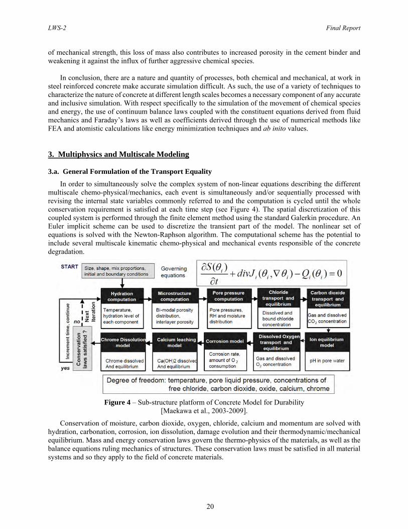
In order to simultaneously solve the complex system of non-linear equations describing the different multiscale chemo-physical/mechanics, each event is simultaneously and/or sequentially processed with revising the internal state variables commonly referred to and the computation is cycled until the whole conservation requirement is satisfied at each time step (see Figure 4). The spatial discretization of this coupled system is performed through the finite element method using the standard Galerkin procedure. An Euler implicit scheme can be used to discretize the transient part of the model. The nonlinear set of equations is solved with the Newton-Raphson algorithm. The computational scheme has the potential to include several multiscale kinematic chemo-physical and mechanical events responsible of the concrete degradation.

Figure 4 – Sub-structure platform of Concrete Model for Durability [Maekawa et al., 2003-2009].

Conservation of moisture, carbon dioxide, oxygen, chloride, calcium and momentum are solved with hydration, carbonation, corrosion, ion dissolution, damage evolution and their thermodynamic/mechanical equilibrium. Mass and energy conservation laws govern the thermo-physics of the materials, as well as the balance equations ruling mechanics of structures. These conservation laws must be satisfied in all material systems and so they apply to the field of concrete materials.

LWS-2 Final Report

21

Given a body, described by the domain Ω ∈ , with a boundary surface S, the notion of continuum mechanics is used to define the balance of a given quantity within that body to be equal to the summation of the point density and the (negative) point sink integrated across the domain, plus the point flux integrated across the surface boundary (Figure 3). This yields the quantity balance formulation of:

d ∙ dS d 20

The divergence theorem is invoked to equate the flux, surface integral to a volume integral, and combine the integrals to yield the general form of

∙ ds ∙ d 21

∙ d 0 22

This integral formulation implies the final general form of

∙ 23

The flux term may then be additively decomposed in order to more accurately characterize the nature

of movement across the boundary. In many cases the flux term is decomposed into convective and diffusive fluxes

∙ ∙ 0 24

There are some cases where the decomposition is the result of a different motivation, such as Maekawa et al. [2009] additive decomposition of flux based on the phase of the transported quantity.

In this section, we recapitulate the governing equations for the stress equilibrium, heat conduction and diffusion and their discretization using the finite element method. The physical process of coupled thermoelastic deformation is governed by the following set of equations.

Stress Equilibrium

The equilibrium of the body is expressed, in a Cartesian coordinate system, as

25

in which

, , , , , 26

is the three-dimensional vector (or tensor) of stress components, with tensile normal stress regarded as positive, and are the body forces. These stress quantities represent the increase over the initial state of stress due to the applied loading and the temperature change.

Strain-displacement relations may be expressed in matrix form as

27

where

LWS-2 Final Report

22

, , , , , 28

is the vector of strain components, and , , is the vector of displacement components.

For the case of the thermoelastic deformations, Hooke’s law for an isotropic material may be written as

29

where the tensor of stress is composed of six different stress components

, , , , , 30

and represent the constant initial and current absolute temperatures, respectively, and is a matrix of elastic constants given by

2 2

0 0

0 00 0

2 0 0 00 0

0

31

with and the Lame modulus and elastic shear modulus of the material, respectively. The thermal stress modulus, is given by

1 2 32

where and are Young’s modulus and Poisson’s ratio of the material and the coefficient of linear thermal expansion. In the case of Thermoelasticity, the Hooke’s law for an isotropic material is

33

where and represent the constant initial and current absolute temperatures, respectively.

Convection-Diffusion

The current framework is based on the conduction/diffusion equation and needs to be extended to more general transport equations, such as those of convection-diffusion. The transient convection-diffusion equation can be written in general form as

D 0 34

where is the transported variable (i.e. the temperature in a thermal problem or the concentration in a pollution transport problem, etc.), is the velocity vector, is the gradient operator, D is the diffusivity matrix, and is the source term.

The presence of convective terms ( ) deprives the standard Galerkin FEM of the best approximation property which it is known to possess in the case of self-adjoint (symmetric) operators. Since the Galerkin discretization of convective terms is akin to a central difference approximation, it tends to produce spurious oscillations. Moreover, an iterative algorithm or an explicit time integration scheme may become unstable.

Several finite element methods have been introduced in numerical literature to avoid this misbehavior [Oñate and Manzan, 2000; Oñate, 2002; Zienkiewicz et al., 2005]. Among the more popular techniques are the following finite element procedures:

LWS-2 Final Report

23

- Artificial Diffusion; - Streamline-Upwind Petrov-Galerkin (SUPG); - Generalized Galerkin, - Taylor-Galerkin; - Characteristic Galerkin (CG), - Galerkin Least Squares (GLS); - Subgrid Scale (SGS); and - Finite Increment Calculus (FIC).

These stabilization techniques are aimed suppress the oscillations or, at least, to keep them small (bounded), and to obtain “stable” finite element solutions for the transient convection-diffusion equation.

Oñate and Manzan [2000] showed that the FIC method, based on a new concept of flow balance over a “finite size” domain, allows reinterpreting and deriving most stabilized methods, at least in steady-state cases, using physical arguments. The FIC method in multidimensions can be written as

2

2

0 35

where denotes the governing differential equations

D 0 36

and the coefficients and are respectively characteristic length and characteristic time parameters.

Moreover, the FIC approach provides a general framework for computing the stabilization parameters in an objective manner. Therefore, the general transport Equation (35) can be discretized using FIC stabilization procedure to model convection-diffusion problems.

3.b. Discretization of equations.

To simultaneously solve the complex system of non-linear equations describing the different multiscale chemo-physical/mechanics, the governing equations for the stress equilibrium, heat conduction and diffusion and their discretization must be implemented using the finite element method. The coupled chemo-thermomechanical process is governed by the following set of equations.

Stress equilibrium (Principle of Virtual Work):

0 37

Heat conduction:

0 38

Diffusion:

0 39

where the displacements , the temperature and the concentration of the diffusing species are the degrees of freedom. The term is the three-dimensional vector (or tensor) of stress components, with tensile normal stress regarded as positive, the surface forces and the body forces.

Fourier’s Law for heat conduction, also referred to as Fick’s for diffusion or Darcy’s law for fluids through porous media, depending on the physical problem or phenomenological transport law, defines the heat flux

in its very general form

LWS-2 Final Report

24

40

where is the thermal temperature-dependent conductivity matrix for concrete. The matrix is a symmetric form due to energy arguments (i.e. , etc.). For the isotropic case, the thermal conductivity is , and in the orthotropic case,

0 00 00 0

. 41

The Fick’s law relates the diffusive flux to the concentration under the assumption of steady state, such as

42

where the diffusion coefficient or diffusivity is analogous to the thermal conductivity . Regarding the characterization of , , , or , one should be aware of their evolution during the temperature evolution but also during the evolution of concentration variables in any diffusion processes occurring in the concrete, such as the cement hydration process. The experimental determination of these properties is usually performed with laboratory procedures.

To solve the above differential equations, the following initial and boundary conditions must be taken into account:

Mechanical

Prescribed displacements: , on ; Pressure: , on ; Volumetric forces in , such as gravity;

Thermal

Prescribed temperatures: , on ; Surface heat flux: , on ; Volumetric heat flux , in , such as the internal heat generated by cement

hydration; Surface heat convection: on where , is the film coefficient and

, is the sink temperature. Heat radiation: on where A is the radiation constant and

is the value absolute zero on the temperature scale.

Diffusional

Prescribed concentrations: , on with 1, ;

Surface diffusion flux: , on with 1,

Volumetric diffusion flux in with 1, ;

LWS-2 Final Report

25

Surface Diffusion convection: on where , is the film

coefficient and , is the sink concentration, with 1, . Diffusion radiation: on where is the radiation

constant and is the value absolute zero on the kth concentration scale, with 1, .

Since there can be several independent concentration variables , … . , , heat can be generated by different chemical and/or physical mechanisms, therefore the volumetric heat flux in can be the addition of several volumetric heat flux terms, such as

, , 43

3.c. Implementation in the user element subroutine UEL.

The user-element subroutine (UEL) is employed to incorporate the governing equations described in the previous section into the finite element code Abaqus. The UEL subroutine allows to the user to use a maximum number of 20 additional degrees of freedom (DOF's) in addition to the existing degrees of freedom (displacement, temperature, etc).

The implementation of the user element subroutine was performed such that the solution is obtained using the linear perturbation procedure for small diplacements, in which the Newton-Raphson method is applied to the set of discretized nonlinear equations

, ,

, 44

,

that corresponds to the discretized equations

, , 0

1Δ

0 45

1Δ

Assuming the state is known at the time t, the equations are solved at the time Δ and for the iteration, the Newton-Raphson method leads to the linear system of equations

46

where the unknowns for displacement, temperature and concentration are

LWS-2 Final Report

26

47

To update the unknowns during each iteration and until the global convergence is satisfied, the Jacobian and the right-hand side (or vector force) were defined in the user element subroutine and returned to the Abaqus solver

with 48

where the unsymmetric stiffness matrix of the system is

49

According to the UEL conventions in Abaqus, the solution variables (displacement, velocity, etc.) are arranged on a node/degree of freedom basis. Therefore, the degrees of freedom of the first node are first, followed by the degrees of freedom of the second node, etc. Following this convention, the flux vector and Jacobian matrix were rearranged at the end of the UEL subroutine. In the current user element implementation, the shape functions of eight types of elements, such as two- and three-dimensional, linear and quadratic elements, were defined (Figure 5):

- 3-node linear triangle - 4-node bilinear quadrilateral - 6-node quadratic triangle - 8-node biquadratic quadrilateral - 4-node linear tetrahedron - 8-node linear brick - 10-node quadratic tetrahedron - 20-node quadratic brick

Based on the number of nodes and dimension of the analysis, the type of element is automatically selected in the subroutine. Therefore different type of elements can be defined in the input file and used simultaneously in the same analysis. Also, based on the number of degrees of freedom defined in the input file, the analysis can solve for displacements, temperature and/or diffusion.

LWS-2 Final Report

27

Figure 5 – Type of elements implemented in the user element subroutine.

The coupling Jacobian terms , , , , and were implemented in the current user element subroutine in case of coupled multiphysics analysis. The Jacobian term was set to zero as the diffusion equations was assumed not depending on displacements.

3.d. Example: Moisture Diffusion Analysis in Concrete.

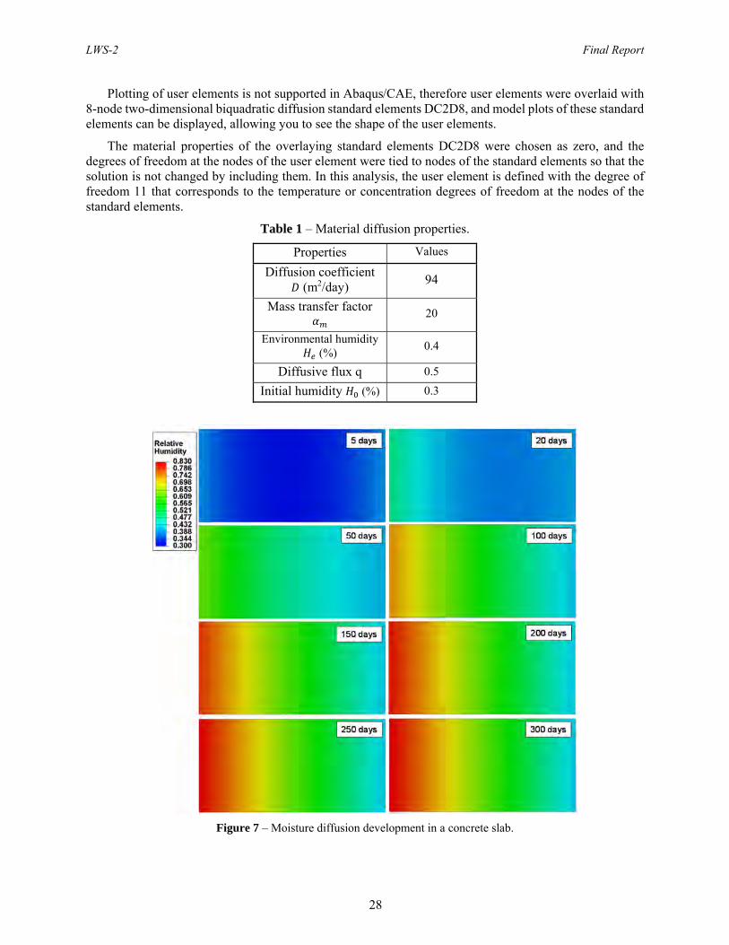
The physical model used in the present study is shown in Figure 6. It is a concrete slab of 40 cm by 80 cm. The concrete slab contains initially has 30% relative humidity (RH). The concrete slab is exposed to 40% RH on the right lateral surface and to a diffusive flux of 94 m2/day on the left lateral surface. The other boundaries are assumed to be sealed. The material parameters used in the example are shown in Table 1.

The mesh is composed of 800 two-dimensional 8-node user elements with quadratic shape functions. Figure 7 shows numerical results from the moisture diffusion analysis. One can see from the color contours in Figure 7 that the moisture is mainly penetrating in the direction towards the right of the concrete slab, and after 250 days the moisture distribution becomes steady state.

Figure 6 – Boundary conditions for the moisture diffusion analysis in a concrete slab.

3 noded triangle 6 noded triangle 4 noded quadrilateral 8 noded quadrilateral

4 noded tetrahedron 10 noded tetrahedron 8 noded brick 20 noded brick

EnvironmentalRelative Humidity:

He=40%

Convective flux:

DiffusiveFlux q

Sealed Boundary

Sealed Boundary

Initial RelativeHumidity H0 = 30%

LWS-2 Final Report

28

Plotting of user elements is not supported in Abaqus/CAE, therefore user elements were overlaid with 8-node two-dimensional biquadratic diffusion standard elements DC2D8, and model plots of these standard elements can be displayed, allowing you to see the shape of the user elements.

The material properties of the overlaying standard elements DC2D8 were chosen as zero, and the degrees of freedom at the nodes of the user element were tied to nodes of the standard elements so that the solution is not changed by including them. In this analysis, the user element is defined with the degree of freedom 11 that corresponds to the temperature or concentration degrees of freedom at the nodes of the standard elements.

Table 1 – Material diffusion properties.

Properties Values

Diffusion coefficient (m2/day)

94

Mass transfer factor

20

Environmental humidity (%) 0.4

Diffusive flux q 0.5

Initial humidity (%) 0.3

Figure 7 – Moisture diffusion development in a concrete slab.

LWS-2 Final Report

29

Since there is an analogy between the heat transfer analysis and the diffusion process inside of a concrete body (see Table 2), this implementation allows the user to sequentially model heat transfer and/or several chemo-physical transport process such as moisture, chloride diffusion, etc.

Table 2 – Corresponding terms in the differential equations for moisture diffusion and heat transfer.

Heat Transfer Moisture

(x,y,t) , ,

K()/c

h

e

s

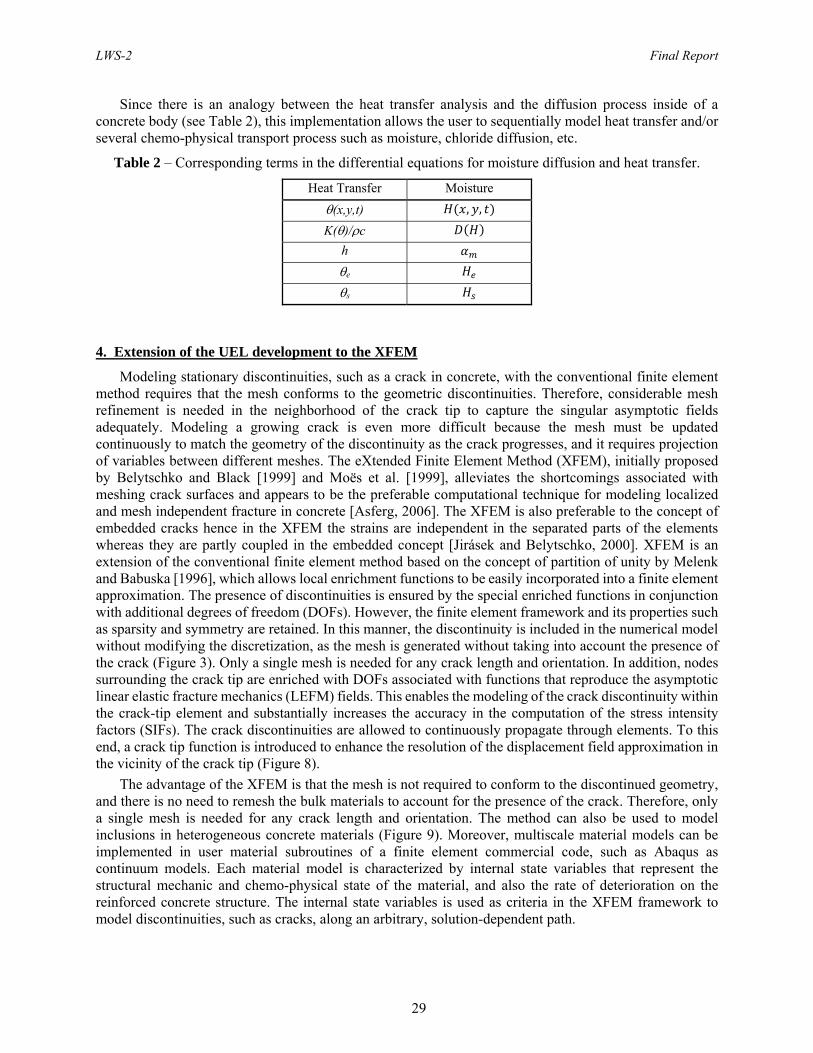
4. Extension of the UEL development to the XFEM

Modeling stationary discontinuities, such as a crack in concrete, with the conventional finite element method requires that the mesh conforms to the geometric discontinuities. Therefore, considerable mesh refinement is needed in the neighborhood of the crack tip to capture the singular asymptotic fields adequately. Modeling a growing crack is even more difficult because the mesh must be updated continuously to match the geometry of the discontinuity as the crack progresses, and it requires projection of variables between different meshes. The eXtended Finite Element Method (XFEM), initially proposed by Belytschko and Black [1999] and Moës et al. [1999], alleviates the shortcomings associated with meshing crack surfaces and appears to be the preferable computational technique for modeling localized and mesh independent fracture in concrete [Asferg, 2006]. The XFEM is also preferable to the concept of embedded cracks hence in the XFEM the strains are independent in the separated parts of the elements whereas they are partly coupled in the embedded concept [Jirásek and Belytschko, 2000]. XFEM is an extension of the conventional finite element method based on the concept of partition of unity by Melenk and Babuska [1996], which allows local enrichment functions to be easily incorporated into a finite element approximation. The presence of discontinuities is ensured by the special enriched functions in conjunction with additional degrees of freedom (DOFs). However, the finite element framework and its properties such as sparsity and symmetry are retained. In this manner, the discontinuity is included in the numerical model without modifying the discretization, as the mesh is generated without taking into account the presence of the crack (Figure 3). Only a single mesh is needed for any crack length and orientation. In addition, nodes surrounding the crack tip are enriched with DOFs associated with functions that reproduce the asymptotic linear elastic fracture mechanics (LEFM) fields. This enables the modeling of the crack discontinuity within the crack-tip element and substantially increases the accuracy in the computation of the stress intensity factors (SIFs). The crack discontinuities are allowed to continuously propagate through elements. To this end, a crack tip function is introduced to enhance the resolution of the displacement field approximation in the vicinity of the crack tip (Figure 8).

The advantage of the XFEM is that the mesh is not required to conform to the discontinued geometry, and there is no need to remesh the bulk materials to account for the presence of the crack. Therefore, only a single mesh is needed for any crack length and orientation. The method can also be used to model inclusions in heterogeneous concrete materials (Figure 9). Moreover, multiscale material models can be implemented in user material subroutines of a finite element commercial code, such as Abaqus as continuum models. Each material model is characterized by internal state variables that represent the structural mechanic and chemo-physical state of the material, and also the rate of deterioration on the reinforced concrete structure. The internal state variables is used as criteria in the XFEM framework to model discontinuities, such as cracks, along an arbitrary, solution-dependent path.

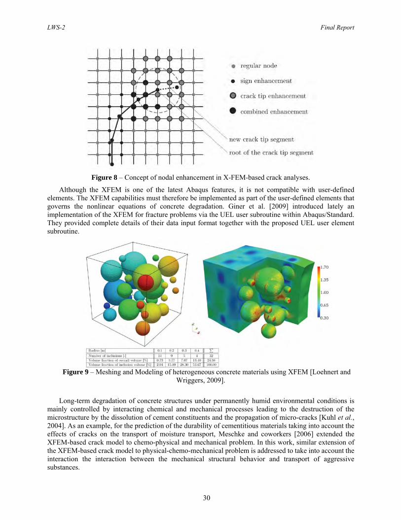
LWS-2 Final Report

30

Figure 8 – Concept of nodal enhancement in X-FEM-based crack analyses.

Although the XFEM is one of the latest Abaqus features, it is not compatible with user-defined elements. The XFEM capabilities must therefore be implemented as part of the user-defined elements that governs the nonlinear equations of concrete degradation. Giner et al. [2009] introduced lately an implementation of the XFEM for fracture problems via the UEL user subroutine within Abaqus/Standard. They provided complete details of their data input format together with the proposed UEL user element subroutine.

Figure 9 – Meshing and Modeling of heterogeneous concrete materials using XFEM [Loehnert and

Wriggers, 2009].

Long-term degradation of concrete structures under permanently humid environmental conditions is mainly controlled by interacting chemical and mechanical processes leading to the destruction of the microstructure by the dissolution of cement constituents and the propagation of micro-cracks [Kuhl et al., 2004]. As an example, for the prediction of the durability of cementitious materials taking into account the effects of cracks on the transport of moisture transport, Meschke and coworkers [2006] extended the XFEM-based crack model to chemo-physical and mechanical problem. In this work, similar extension of the XFEM-based crack model to physical-chemo-mechanical problem is addressed to take into account the interaction the interaction between the mechanical structural behavior and transport of aggressive substances.

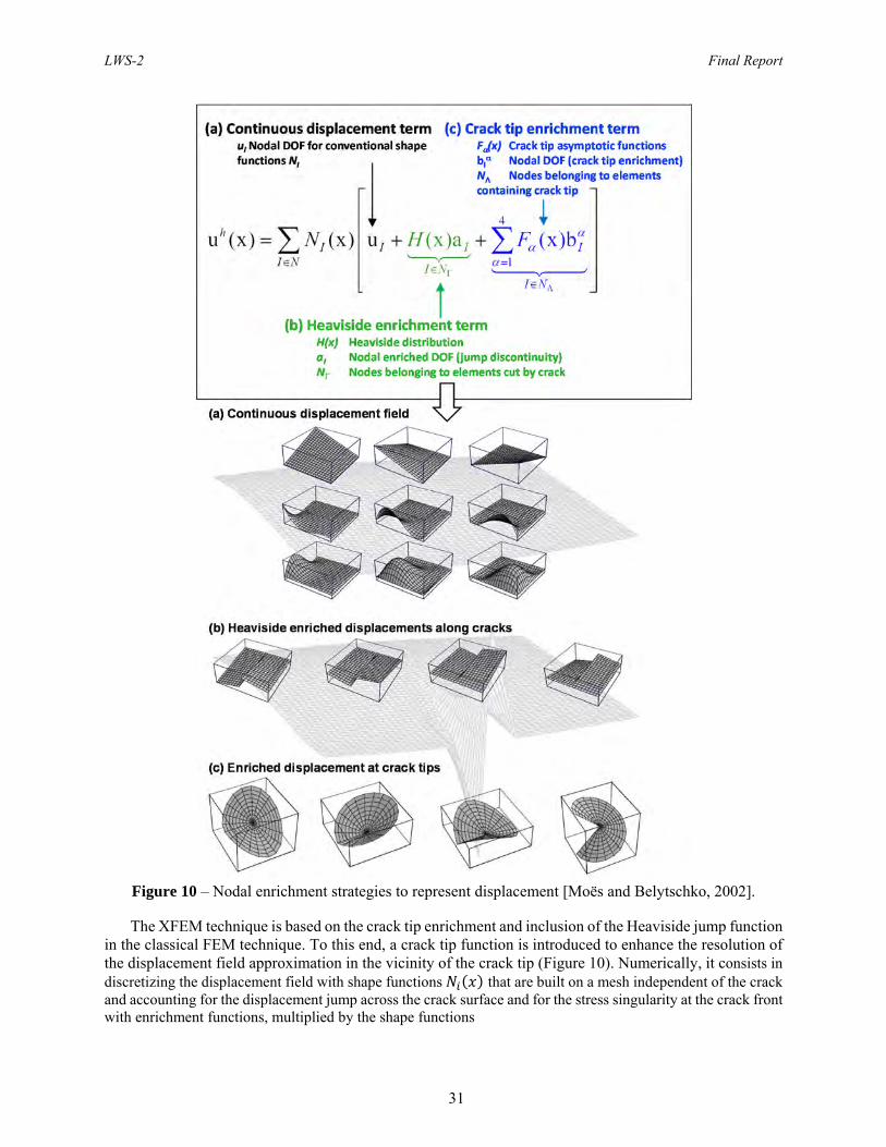
LWS-2 Final Report

31

Figure 10 – Nodal enrichment strategies to represent displacement [Moës and Belytschko, 2002].

The XFEM technique is based on the crack tip enrichment and inclusion of the Heaviside jump function in the classical FEM technique. To this end, a crack tip function is introduced to enhance the resolution of the displacement field approximation in the vicinity of the crack tip (Figure 10). Numerically, it consists in discretizing the displacement field with shape functions that are built on a mesh independent of the crack and accounting for the displacement jump across the crack surface and for the stress singularity at the crack front with enrichment functions, multiplied by the shape functions

LWS-2 Final Report

32

∈ ∈

∈

50

The step function with a changing sign across the crack, enriches the nodes completely cut by the crack (set ). It is convenient to define it with the help of the signed distance function to the crack :

sign 51

The four following branch functions enrich the nodes with a distance to the front inferior to a prescribed enrichment radius (set ):

√ cos2

, √ sin2

, √ sin2

sin , √ cos2

sin 52

where , is a polar coordinate system with origin at the crack tip, and N x are the standard finite element shape functions. The enrichment coefficients and are associated with nodes and is the number of coefficients for node ; it is chosen to be four for all nodes around the crack tip and zero at all other nodes. The implementation of the XFEM is performed through the user element subroutine UEL that was developed by Giner et al. [2009]. As all user elements, this implementation is limited by the information passed in the UEL subroutine by the commercial code Abaqus, but it also takes advantage of many features available in this code, such as the solver, the boundary conditions, the pre-processing and post-processing, etc. The main disadvantage is that user elements cannot be fully post-processed as standard elements in Abaqus, and as mentioned above, a Python script is needed to generate element information in the output database. In this implementation, all enriched elements are defined by a 4 node user element with 12 degrees of freedom (DOFs) per node. Table 3 gives the description of DOFs according to the Abaqus convention. In this 2D analysis, DOFs 3 and 4 are used as additional DOFs within the Heaviside and crack tip enriched elements. DOFs 5–7 and 11–15 are only active in the crack tip enriched elements. The different integration steps in the XFEM implementation are identified in the chart form in Figure 11 and are based on the integration procedure performed by Giner et al. [2009], in which displacements are the only degrees of freedom.

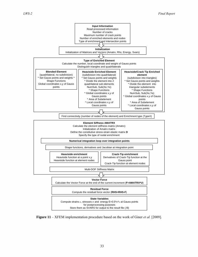
LWS-2 Final Report

33

Figure 11 – XFEM implementation procedure based on the work of Giner et al. [2009].

Input InformationRead processed information

Number of cracksMaximum number of crack points

Number of enriched elements and nodesType of enrichment and intersection points

InitializationInitialization of Matrices and Vectors (Amatrx, Rhs, Energy, Svars)

Type of Enriched ElementCalculate the number, local coordinate and weight of Gauss points

Distinguish triangles and quadrilaterals

Blended Element(quadrilateral, no subdivision)

* Set Gauss points and weights * Shape Functions

Global coordinates x,y of Gauss points

Heaviside Enriched Element(subdivision into quadrilateral)

* Set Gauss points and weights* Divide the element into 2 quadrilateral sub elements

NumSub, Sub(Xe,Ye)* Shape Functions

* Global coordinates x,y ofGauss points

* Area of Subelement* Local coordinates x,y of

Gauss points

Heaviside/Crack Tip Enriched element

(subdivision into triangles)* Set Gauss points and weights

* Divide the element into triangular subelements

* Shape FunctionsNumSub, Sub(Xe,Ye)

* Global coordinates x,y of Gauss points

* Area of Subelement* Local coordinates x,y of

Gauss points

Find connectivity (number of nodes of the element) and Enrichment type (TypeX)

Element Siffness AMATRXCalculate the element stiffness matrix (Amatrx)

Initialization of Amatrx matrixDefine the constitutive stress-strain elastic matrix D

Specify the type of nodal enrichment

Shape functions, derivatives and Jacobian at integration point

Heaviside enrichment Heaviside function at a point x,y

Heaviside function at element nodes

Crack-Tip enrichment Derivatives of Crack-Tip function at the

Gauss pointCrack-Tip function at element nodes

Multi-DOF Stiffness Matrix

Numerical integration loop over integration points

Vector ForceCalculate the Vector Force at the end of the current increment (F=AMATRX*U)

Residual ForceCompute the residual force vector (RHS=RHS-F)

State VariablesCompute strains , stresses and energy E=0.5** at Gauss points

for postprocessing purposesStore them as SVARS for output to the result file (.fil)

LWS-2 Final Report

34

Different numerical implementation aspects must be considered to achieve this goal of coupling the classical elastic fracture XFEM to other phenomena:

First, governing equations must be coupled, as temperature dependence is assumed to be the linking variable that couples the different governing equations;

Governing equations are discretized and solved using the Galerkin finite element methodology and then implemented in the user element subroutine UEL;

Then, the numerical application of the enrichment strategy is applied to all degrees of freedom, which are the mechanical displacement, the temperature, and the concentration variables.

Enriched elements are divided in sub-elements to perform the quadrature integration while taking crack discontinuities into account. New boundary conditions within enriched elements, such as flux discontinuities, are considered at the crack interface.

Finally, the geometrical and material response characterized by displacements, temperature and is used to evaluate the aging degradation of concrete in a post-processing step.

In this work, the same XFEM integration procedure can be applied with an extension of the number of DOF to include the temperature and concentration variables. The XFEM implementation can be either performed on 2D quadrilateral elements that can be divided into triangular or quadrilateral subelements, 3D brick elements that can be divided into tetrahedral or brick subelements, depending on the type of enrichment functions (blended, Heaviside or crack-tip).

Therefore, an identical nodal enrichment strategy for displacement is used to represent local (discontinuous) temperature and n concentration variables. In analogy to the partitioning of the displacement field u, the enrichment concept can also be applied to the incorporation of the temperature and n concentration variables ( 1, ) within cracks

⋮ ⋮∈ ⋮∈ ⋮

∈

53

This enriched (X-FEM) modeling concept allows the incorporation of temperature and diffusive transport of concentrations within cracks.

Figure 12 – Nodal enrichment strategies to represent concentration variables within X-FEM.

X+

X‐

H(x)=+1 above crack X+

H(x)= ‐1 above crack X‐

LWS-2 Final Report

35

Example: Crack opening using a UEL-XFEM subroutine

To illustrate the implementation of the XFEM in Abaqus, input files with crack and element information were created to model a portion of a cracked finite strip loaded under uniform normal stress. Two different meshes are considered, a coarse mesh and a fine mesh (Figures 14 and 15). All elements that contained at least one enriched node are defined by the UEL-XFEM element subroutine. All other elements are 4-node standard elements from the Abaqus element library. Additional standard 4-node linear elements with a negligible stiffness have been inserted in the XFEM analysis for the purpose of plotting the deformed shape. These elements have negligible stiffness, are superimposed on every enriched element, and share the same node connectivity with enriched elements. Nodes on both sides are constrained in the direction and nodes at the bottom are fully constrained. A displacement is applied at the nodes at the top. The crack location and the enriched nodes for both the Heaviside and crack tip enrichment are shown in the sketch on the top left of Figures 8 and 9.

Table 3 – Degrees of freedom in Abaqus.

Degrees of Freedom Description 1 Displacement 2 Displacement 3 Displacement 4 Rotation about axis 5 Rotation about axis 6 Rotation about axis

7 Warping amplitude of

beam section

11-15 First and successive temperatures in shell and plate elements

The contour plots of the Mises stress distribution using the XFEM implementation are shown on the top right of both Figures 14 and 15. The crack does not appear on each figure but its effects on the solution are included in the user enriched elements. Elements with low stress values (in blue) are overlay elements with negligible stiffness that help to visualize the discretization of the solution and its deformed shape. A standard FE solution with a discontinuity representing the crack has also been performed for comparison purposes (bottom left and right of Figures 8 and 9) with the XFEM solution. On the bottom right, elements along the crack discontinuity have been removed from the display to be able compare stress distribution with that of the XFEM analysis. We can observe that the XFEM stress distribution (top right) is very similar to the FE solution (bottom right) for both coarse and fine meshes (Figures 14 and 15), which means that the effects of the crack discontinuity are well included in the Heaviside and crack tip enrichments functions.

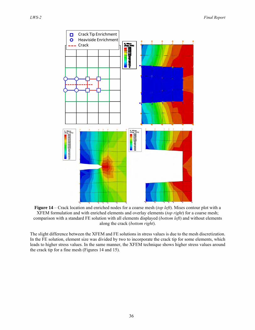
LWS-2 Final Report

36

Figure 14 – Crack location and enriched nodes for a coarse mesh (top left). Mises contour plot with a XFEM formulation and with enriched elements and overlay elements (top right) for a coarse mesh;

comparison with a standard FE solution with all elements displayed (bottom left) and without elements along the crack (bottom right).

The slight difference between the XFEM and FE solutions in stress values is due to the mesh discretization. In the FE solution, element size was divided by two to incorporate the crack tip for some elements, which leads to higher stress values. In the same manner, the XFEM technique shows higher stress values around the crack tip for a fine mesh (Figures 14 and 15).

Crack Tip EnrichmentHeaviside EnrichmentCrack

LWS-2 Final Report

37

Figure 15 – Crack location and enriched nodes for a fine mesh (top left). Mises contour plot with a XFEM formulation and with enriched elements and overlay elements (top right) for a coarse mesh;

comparison with a standard FE solution with all elements displayed (bottom left) and without elements along the crack (bottom right).

5. Aging Degradation of Concrete

The last aspect of this multiscale modeling approach is to develop an integrated model able to simulate the long-term durability of reinforced concrete structures used in NPP facilities. Initially, predictive methodologies already available in concrete codes are used for assessing the aging degradation process. Then, it is essential in these predictive methodologies to obtain the information developed in multiphysics analyses on the estimation of (i) the concrete degradation due to chemical and physical-mechanical stresses; and (ii) the water and flow properties during variably saturated flow conditions in (cracked) degraded

Heaviside EnrichmentCrack Tip Enrichment

Crack

LWS-2 Final Report

38

concrete. Finally, it is of great interest to incorporate the XFEM element-by-element crack propagation information in the durability model and to assess its damage effect on the long term structural performance. Data of experimental measurements of degradation in structures reported in the literature can be used to calibrate and validate the durability model.

Service life of a concrete structure is defined in different ways depending on the degree of cumulative damage and identified aging processes (Figure 13). Some of these definitions are:

Time from construction until when the water saturation, chloride content at the reinforcement, frost damage, etc., are high enough to initiate concrete degradation and steel corrosion;

Time from construction to time at which signs of distress are visible/observable (acceptable degradation state);

Time from construction to time at which the member/component/structure is considered to be functionally unacceptable or unsafe (service life).

5.a. Damage modeling.

The durability model is based on the damage degradation of material properties of concrete. Continuum damage mechanics (CDM) offer a means of modeling at the macroscopic level the material damage that occurs at the microscopic level. Development of a damage-based model requires definition of a damage evolution equation that characterizes the rate at which material damage is accumulated and eventually the orientation of the damage. The damage is inserted in the model as an internal state variable (ISV) that deteriorates the mechanical properties of concrete. The material response of this model describes the macroscopic response of a body of concrete that is many times the size of individual pieces of aggregate.

Figure 13 – Durability modeling methodology to evaluate service life of concrete structures.

The damage theory is based on the continuum damage mechanics (CDM). The model is based on the

theory of rate-independent elastoplasticity with damage. The model is incorporated into the finite element code Abaqus as a user defined material model (UMAT-interface within UEL).

Damage in CDM models is generally represented by the void volume fraction as it was initially proposed by Kachanov [1958] using the concept of effective stress, . This theory is based on considering a fictitious undamaged configuration in which the damage is taken into account by measuring the reduction in the resistant area due to cracks beginning and spreading of the actual damaged configuration:

1

2

3

Deg

ree

of c

um

ula

tive

dam

age

Time

Cracking

Acceptable degradation rate

Water saturation,Chloride penetrationFrost damage, etc.Initiation period

Propagation periodReinforcement CorrosionChemo-physical attack

XFEM

LWS-2 Final Report

39

1, 54

where is the stress in the actual damage configuration, and and are the resistant area of the undamaged and damage configurations, respectively. The damage value ranges from 0, in the case of an undamaged material, to 1, in the case of a fully damaged material. Since the damaging mechanisms are different in uniaxial tension and compression experiments for concrete materials, the damage variable

is additively decomposed into two parts, for tension and for compression

, 55

where α and α are weighting coefficients [Mazars and Pijaudier-Cabot, 1989].

Here, to represent the material damage in concrete, the reduced stiffness is described as a function of temperature, radiation, and/or other diffusion variable, such as leaching, in addition of being a function of void volume fraction that represents the pores and microcracks in a unit volume.

The thermo-chemical material degradation at elevated temperatures (mainly due to micro-cracking and cement dehydration) lead to additional reduction of the material strength properties and is represented by the damage variable . Its contribution to the total reduction of the material strength properties is defined by [Pomaro et al., 2011]

1 1 56

total damage of the mechanical and thermo-chemical damages acting at the same time is therefore multiplicative, i.e. the total damage is defined by

1 1 1 . 57

Pomaro et al. [2011] upgraded this damage model definition by assuming that the nuclear radiation can generate a specific damage process in addition to the mechanical and thermo-mechanical ones so that the above equation becomes

1 1 1 1 . 58

This material damage in the concrete structure leads to a degradation of material stiffness, as observed on the macroscale level, and it is represented by

1 59

where is the material stiffness of the undamaged concrete structure.

The material damage in the concrete structure leads to a degradation of material stiffness, as observed on the macroscale level, and it is represented by

E E 1 D , 60

where is the material stiffness of the undamaged concrete structure. The damage variable is defined by assuming that the nuclear radiation can generate a specific damage process in addition to the mechanical and thermo-mechanical ones [Pomaro et al., 2011] so that the above equation becomes

D 1 1 D 1 D 1 D 61

Lately it is widely realized that concrete structures are no longer maintenance-free. As a result, evaluation techniques for diagnostic inspection are in great demand in concrete engineering. As a detailed inspection of a concrete structure in service, core samples are usually drilled out and then both chemical and physical properties are measured. Concerning mechanical property of the physical property, the compressive strength and the modulus of elasticity (Young’s modulus) are normally determined by conducting a uniaxial compression test. These values are then compared, if possible, with those of the

LWS-2 Final Report

40

specification. Otherwise, there is no qualified procedure to estimate mechanical properties responsible for the durability and the deterioration of concrete. In most cases, only the strength is evaluated whether the obtained value is good enough against designed stress.

5.b. Fatigue modeling

A MultiStage Fatigue (MSF) model initially developed for aluminum cast alloys (Horstemeyer et al., 2001; McDowell et al., 2003, Xue et al., 2007) and further enhanced for magnesium alloys (El Kadiri et al., 2006) is used here to predict the fatigue life of PM alloys. Since the PM alloys have similar microstructures and inclusions/defects, the modeling framework is inferred to be general enough to capture the fatigue behavior of these various PM alloys. Similarly to metals, material aging of concrete is generally associated with changes over time in mechanical properties such as creep, modulus, and ultimate compressive and tensile strengths. Moreover, the behavior of concrete is also highly nonlinear, having low tensile strength, shear stiffness and strength that depend on crack widths, and a confinement-dependent compressive elasto-plasticity. Structural aging, on the other hand, is the combined effects of changes in the time-dependent material properties, the prior physical changes resulting from the past environmental and loading history of the concrete structure, and the current environmental conditions and applied loads [Rashid et al., 2011].

The high fidelity multistage fatigue (MSF) model predicts the amount of fatigue cycling required to cause the appearance of a measurable crack, the crack size as a function of loading cycles. The model incorporates microstructural features to the fatigue life predictions for incubation, microstructurally small crack growth, and long crack growth stages in both high cycle and low cycle regimes.

The microstructure-based MSF model incorporates different microstructural discontinuities effect (pores, inclusions, etc.) on physical damage progression. This model partitions the fatigue life into three stages based on the fatigue damage formation and propagation mechanisms:

- crack incubation (INC), - microstructurally small crack (MSC) and physically small crack (PSC) growth, and - long crack (LC) growth.

The total fatigue life is decomposed into the cumulative number of cycles spent in several consecutive stages as follows:

62

where is the number of cycles to incubate a crack at a micronotch that includes the nucleation of crack-like damage and early crack propagation through the region of the micronotch root influence; is the number of cycles required for propagation of a microstructurally small crack with the crack length a. The crack range, ai < a < kDCS, with the DCS defined as the dendrite cell size, and k as the non-dimensional factor that is representative of a saturation limit for the encountering of a 3-D crack front with sets of microstructural discontinuities. The value is the number of cycles required for LC propagation for crack length a > (10–20) DCS, depending on the amplitude of loading and the corresponding extent of microplasticity ahead of the crack tip. This stage of crack extension is commonly characterized using standard fatigue crack growth experiments, / versus . Finally is the total fatigue life.

To study the damage incubation life as a function of local plastic deformation, a modified Coffin–Mansion law was implemented based on the non-local maximum plastic shear strain, i.e.:

Δ2

63

where is the non-local maximum plastic shear strain amplitude around the inclusion calculated using an average of maximum plastic shear strain over an area approximately one percent of the inclusion area, and CINC and are the linear and exponential coefficients in the modified Coffin–Mansion law at the micronotch. The Paris Law is used to define the long crack growth rate (Paris et al., 1961). This implies that:

LWS-2 Final Report

41

64

where A is the crack growth parameter and m the exponent in Paris Law, ΔK is the stress intensity factor, N the number of cycles, and logA is defined as a constant.

The Multi-Stage Fatigue model was implemented in the subroutine Abaqus user output variable subroutine UVARM. It calculates the fatigue lives , , and at each material point using the stress and strain amplitudes provided by the fatigue analysis, and store the values in user output variables UVARi. This MSF durability model can easily be integrated in the current Abaqus UEL subroutine via a user-defined post-processing subroutine that generates element output at all material calculation points of elements. This subroutine is called in UEL at the end of each increment when the solution has converged. The user subroutine can obtain the values of all nodal and material point quantities that are necessary to the durability model. The user subroutine calculates at the end of each increment the durability values at each material point and store them in user output variables (UVARi), which are added to the state variables SVARS of UEL to be available for post-processing in Abaqus Visualization module through a Python script.

6. Conclusions

In this work, we developed a numerical procedure for the implementation of the multiscale and multiphysics platform within the commercial FE code Abaqus for two- and three-dimensional transport process problems in concrete structures. In this user element subroutine UEL, multiple transport processes that occur in concrete and lead to the degradation, such as the ones presented in the literature review, can be user-defined and solved simultaneously with mechanical and thermal analyses. The UEL user element subroutine was verified and validated in Abaqus for eight different two- and three-dimensional, linear and quadratic, finite elements. The multiphysics formulation was theoretically extended to the XFEM theory, in which it was shown that the same Heaviside and crack tip enrichment functions for displacements can be used to discretize the temperature and concentration variables in order to model weak and strong discontinuities. Therefore, the current user element implementation constitutes a future platform for a multiphysics XFEM approach as it can be used for the numerical integration of the subelements that results from the decomposition of XFEM elements. The modeling of concrete deterioration of mechanical properties due transport processes was theoretically formulated within the framework continuum damage mechanics, in which an internal state variable representing the total damage and the sum of all damage mechanisms was introduced. The total damage variable and the damaged material stiffness were then finally incorporated in a Multi-Stage fatigue model for the assessment of aging degradation of concrete. References

Abaqus, Version 6.11-1, User’s Manual, SIMULIA, Providence, RI, 2009. Abarbanel, S., & Ditkowski, A. “Multi-dimensional asymptotically stable finite difference schemes for

the advection-diffusion equation,” Computers & Fluids, Vol. 28, pp. 481–510, 1998. Asahina, D., and Bolander, J.E., “Voronoi-based discretizations for fracture analysis of particulate

materials. Powder Technology, Vol. 213, pp. 92-99, 2011. Asferg, J.L., Modeling of Concrete Fracture Applying the eXtended Finite Element Method, PhD Thesis,

Department of Civil Engineering, Technical University of Denmark, 2006. Bazant, Z.P., and Thonguthai, W., “Pore pressure and drying of concrete at high temperature,” Journal of

the Engineering Mechanics Division, ASME,, Vol. 104, No. 5, pp. 1059–1079, 1978. Bazant, Z.P., and Najjar, L.J., “Nonlinear water diffusion in nonsaturated concrete,” Materials and

Structures, Vol. 5, No. 1, pp. 3–20, 1972.

LWS-2 Final Report

42

Bejaoui, S., Sercombe, J., · Mugler, C., and. Peycelon, H., “Modelling of Radionuclide Release from a Concrete Container,” Transport in Porous Media, Vol. 69, pp. 89–107, 2007.

Belytschko, T., and T. Black, T., `”Elastic Crack Growth in Finite Elements With Minimal Remeshing,'' International Journal for Numerical Methods in Engineering, Vol. 45, No. 5, pp. 601-620, 1999.

Bonaccorsi, E., Merlino, S., and Kampf, A.R., “The crystal structure of tobermorite 14 Å (Plombierite), a C-S-H phase,” Journal of the American Ceramic Society, Vol. 88, pp. 505–512, 2005.

Cady, P.D. and Weyers, R.E., “Predicting Service Life of Concrete Bridge Decks Subject to Reinforcement Corrosion,” ASTM Special Technical Publication, No. 1137, pp. 328–338, 1992.

Costa, A., and Appleton, J., “Chloride penetration into concrete in marine environment – Part I: Main parameters affecting chloride penetration,” Materials and Structures, Vol. 32, No. 4, pp. 252–259, 1999.

Costa, A., and Appleton, J., “Chloride penetration into concrete in marine environment – Part II: Prediction of long term chloride penetration. Materials and Structures, Vol. 32, No. 6, pp. 354–359, 1999.

Cerny, R., and Ravnanikova, P., Transport Processes in Concrete. New York, NY, Spon Press, 2002. DiMaggio, F.L., and Sandler, I.S., “Material models for granular,” Journal of Engineering Mechanics,

ASCE, Vol. 97, EM3, pp. 935–950, 1971. Drucker, D.C. and Prager, W., “Soil Mechanics and plastic analysis or limit design,” Quarterly of Applied

Mathematics, Vol. 10, No. 2, pp. 157–165, 1952. Fillmore, D.L., Literature Review of the Effects of Radiation and Temperature on the Aging of Concrete,

Technical Report INEEL/EXT-04-02319, Idaho National Laboratory (INL), September 2004. Fossum, A.F., and Brannon, R.M., 2004, The Sandia Geomodel: Theory and User’s Guide, Sandia Report

SAND2004-3226 UC-405. Fries T.P., and Belytschko T., “The intrinsic XFEM: a method for arbitrary discontinuities without

additional unknowns, “International Journal for Numerical Methods in Engineering,; Vol. 68, No. 13, pp. 1358–1385.

Fujiwara, K., Ito, M., Sasanuma, M. Tanaka, H., Hirotani, K., Onizawa, K. Suzuki,M. and Amezawa, H., “Experimental Study of the Effect of Radiation Exposure to Concrete,” 20th International Conference on Structural Mechanics in Reactor Technology (SMiRT 20), Espoo, Finland, August 9-14, 2009.

Funahashi, M., “Predicting corrosion free service life of a concrete structure in a chloride environment,” ACI Materials Journal, Vol. 87, No. 6, pp. 581–587, 1990.

Gawin, D., Pesavento, F. and Schrefler, B.A., “Hygro-Thermo-Chemo-Mechanical Modelling of Concrete at Early Ages and Beyond. Part II: Shrinkage and Creep of Concrete,” International Journal for Numerical Methods in Engineering, Vol., 67, pp. 332–363, 2006.

Giner, E., Sukumar, N., Tarancón, J.E., and Fuenmayor, F.J., “An Abaqus Implementation of the Extended Finite Element Method, Engineering Fracture Mechanics, Vol. 76, No. 3, pp 347–368, 2009.

Hofstetter, G., Simo, J.C., and Taylor, R.L., “A Modified Cap-model: Closest Point Solution Algorithms,” Computers & Structures, Vol. 46, pp. 203–214, 1993

Kachanov, L.M., “Time of the Rupture Process under Creep Conditions,” IVZ Akad. Nauk. S.S.R. Otd. Tech. Nauk., 8, pp. 26–31, 1958.

Klute, A. (1952), “A numerical method for solving the flow equation for water in unsaturated material,” Soil Science, Vol. 73, pp. 105-116.

Kuzmin, D. (2010), “A Guide to Numerical Methods for Transport Equations,” University Erlangen-Nuremberg. Manuscript available online at http://www.mathematik.uni-dortmund.de/_kuzmin/Transport.pdf

Loehnert and Wriggers, “On the eXtended Finite Element Method,” Ljubljana, 2009.

LWS-2 Final Report

43

Lowes, L.N., “Finite Element Modeling of Reinforced Concrete Beam-Column Bridge Connections,” PhD Thesis, University of California at Berkeley, 1999.

Maekawa, K., Ishida, T., & Kishi, T., Multi-Scale Modeling of Structural Concrete, New York, NY, Taylor & Francis, 2009.

Maekawa, K., Ishida, T., and Kishi, T., “Multi-scale Modeling of Concrete Performance -Integrated Material and Structural Mechanics,” Journal of Advanced Concrete Technology, Vol. 1, No. 2, pp. 91–126, 2003.

Majorana, C.E., Salomoni, V.A. and Schrefler, B.A. “Hygrothermal and mechanical model of concrete at high temperature,” Materials and Structures, Vol. 31, pp. 378–386, 1998.

Mazars, J., Pijaudier-Cabot, G., “Continuum Damage Theory–Application to Concrete,”J. Eng. Mech., ASCE, Vol., 115, pp. 345–365, 1989.

Meschke, G., Dumstorff, P., Fleming, W., and Jox, S., “Numerical analysis of crack propagation in concrete structures using X-FEM,” In G. Meschke, R. deBorst deBorst deBorst, H.A. Mang, and N. Bicanic, editors, Computational modeling of concrete structures (EURO-C 2006), pp 157 –166, Leidon/London /NewYork/Philadelphia/ Singapore, 2006. A.A. Balkema.

Moës, N. and T. Belytschko, “Extended Finite Element Method for Cohesive Crack Growth. Engineering Fracture Mechanics, Vol. 69, pp. 813–833, 2002.

Naus, D. J. , Concrete Materials and Structures - Aging and Life Beyond 40 Years, 60 Years, NRC, DOE Workshop on U.S. Nuclear Power Plant Extension R&D, Bethesda, 2008.

Naus, D. J. (2009), “Management of Aging in Nuclear Power Plant Concrete Structures,” JOM, Vol. 61, No. 7, pp. 35–41.

Naus, D.J., “A Compilation of Elevated Temperature Concrete Material Property Data and Information for Use in Assessments of Nuclear Power Plant Reinforced Concrete Structures,” NUREG/CR-7031, USNRC, Washington, D.C., December 2010.

Ng and Dai, “Investigation of Fracture Behavior of Heterogeneous Infrastructure Materials with Extended-Finite-Element Method and Image Analysis,” Journal of Materials in Civil Engineering, Vol. 23, pp. 1662–1671, 2011.

Oñate, E., “Multiscale computational analysis in mechanics using finite calculus: an introduction,” Comput. Methods Appl. Mech. Engrg., Vol. 192, pp. 3043–3059, 2002.

Oñate, E., and Mazan, M., “Stabilization Techniques for Finite Element Analysis of Convection-Diffusion Problems,” International Center for Numerical Methods in Engineering, Publication CIMNE Nº-183, February 2000.

Pellenq, R.J., M-, Lequeux, N., and van Damme, H. (2008), “Engineering the bonding scheme in C-S-H: The iono-covalent framework,” Cement and Concrete Research, Vol. 38, pp. 159–174.

Pomaro, B., Salomoni, V.A., Gramegna, F., Prete, G., Majorana, C.E., “Radiation damage evaluation on concrete within a facility for Selective Production of Exotic Species (SPES Project), Italy.” Journal of Hazardous Materials, Vol.194, pp. 169–177, 2011.

Powers, T.C., “Structure and Physical Properties of Hardened Portland Cement Paste,” Journal of American Ceramic Society, Vol. 41, No. 1, pp. 1–6, 1958.

Rabczuk, T., and Wall, W.A., Extended Finite Element and Meshfree Methods, Technical University of Munich, Munich, 2006.

Rashid, M.M., and Sadri, A., “The partitioned element method in computational solid mechanics,” Computer Methods in Applied Mechanics and Engineering, Vol. 237–240, 1 pp. 152–165, 2012.

Rashid, J.Y.R.; James, R.J.; Dunham, R.S., “Modeling and analysis of aging behavior of concrete structures in nuclear power plants,” Anatech (United States); Société Française d'Énergie Nucléaire (SFEN), 75 - Paris (France), Vol.42, No. 39, 2011.

Richardson, M. (2002), Fundamentals of Durable Reinforced Concrete. New York, NY, Spon Press.

LWS-2 Final Report

44

Richardson, I. G. (2008), “The calcium silicate hydrates,” Cement and Concrete Research, Vol. 38, No. 2, pp. 137–158.

Rodriguez, J., Ortega, L., Casal, J. and Diez, J. (1996), “Corrosion of reinforcement and service life of concrete structures,” C. Sjostrom (ed) Durability of Building Materials and Components, Vol. 7.

Sukumar N, Chopp DL, Moës N, Belytschko T., “Modeling holes and inclusions by level sets in the extended finite-element method,” Computer Methods in Applied Mechanics and Engineering, Vol. 190, pp. 6183–6200, 2001.

Snyder, K.A., and Bentz, D.P., Doubling Concrete Service Life, 2009 BFRL Project Description, 2009. Tuutti, K., Corrosion of Steel in Concrete, Swedish Cement and Concrete Research Institute, Stockholm,

1982. Zemajtis, J., Weyers, R.E., and Sprinkel, M.M., “An Evaluation of the Performance of Epoxy-Coated

Reinforcing Steel in Concrete Exposure Specimens. (Report No. VTRC 99-CR2). Virginia Transportation Research Council, Charlottesville, 1998.

LWS-2 Final Report

45

Appendix A

Discretization of governing equations and implementation in UEL subroutine

Principle of Virtual Work

Using the Principle of Virtual Work (PVW), we write the weak form equation:

A. 1

The finite element approximation for displacement and virtual displacements leads to

, and , A. 2

where , are the shape functions, (or basis functions, and, occasionally interpolation functions).

12

and A. 3

where the matrix is defined by

0 0

0 0

0 0

0

0

0

A. 4

The principle of virtual work (PVW) is defined by:

A. 5

By eliminating the displacements in the above equation, we obtain

A. 6

The problem is nonlinear due to the material nonlinearities. Therefore we have: and the finite element equation to solve is:

A. 7

The system of equations is the out of balance/residual vector force. is a set of non-linear equations in u that must be solved using the Newton-Raphson method. The Equation (16) is usually presented in the following form

LWS-2 Final Report

46

0 A. 8

With the element stiffness matrix

A. 9

and where

A. 10

is the load vector composed of the vector of actual surface forces and body forces , and the thermal vector which represents fictitious forces for modeling thermal expansion:

A. 11

A. 12

A. 13

Heat Conduction

In the heat conduction problem, the energy balance

. 14

where is the material time derivative of the internal energy

A. 15

Fourier Law’s, also referred to as Fick’s, or Darcy’s law depending on the physical problem, defines the heat flux in its very general form

A. 16

where is the thermal temperature-dependent conductivity matrix for concrete. The matrix is a symmetric form due to energy arguments (i.e., , etc.). For the isotropic case, the thermal conductivity is , and in the orthotropic case,

0 00 00 0

. A. 17

Regarding the characterization of , , , one should be aware of their evolution during the temperature evolution but also during the evolution of concentration variables in any diffusion processes occurring in the concrete, such as the cement hydration process. The experimental determination of these properties is usually performed with laboratory procedures.

LWS-2 Final Report

47

To solve the above differential equation for heat conduction, one needs initial and boundary conditions:

Prescribed temperatures: , on Surface heat flux: , on Volumetric heat flux, such as the internal heat generated by cement hydration: r r x, t in V Surface convection: on where , is the film coefficient and

, is the sink temperature. Radiation: on where A is the radiation constant and is the

value absolute zero on the temperature scale.

Using the divergence theorem

. div A. 18

The heat conduction equation (17) becomes

0 A. 19

for any body volume , which leads to the strong form equation

0 A. 20

And the balance residual equation is

0 A. 21

The next step equalizes the number of derivatives on the test and trial functions. The balance residual equation with the weighted balance residual reads

0 A. 22

On the second term

A. 23

The integration by parts in the case of a multidimensional integral is generalized in the divergence theorem. We may anticipate that the term is the result of the chain rule applied to the vector such as

A. 24

The surface integral can be decomposed into several terms

A. 25

LWS-2 Final Report

48

Because the term is unknown on surface , we choose the test function must satisfy the condition 0 for ∈ , which leads to

0. A. 26

Switching from to , the left hand side term in Equation (27b) becomes

A. 27

The heat flux passing through is known. Therefore if we attempt to satisfy this boundary condition in a weighted residual sense, we write

0 A. 28

Similarly on the surface

0 A. 29

and on the surface

0 A. 33

If we had these three boundary conditions to weighted balance residual 0, we obtain

A. 34

The underlined surface terms cancel with the surface integral in (34) and we arrive at

0 A. 35

where is an arbitrary variational field (test function) satisfying the essential boundary conditions with 0 for ∈ . The body is approximated geometrically with finite element, so the temperature is

also interpolated using the shape functions , as

, A. 36

where are the nodal temperatures. The Galerkin approach assumes , the variational field, is interpolated by the same functions

, . A. 37

First- and second-order polynomial in one, two, three dimensions are used for the shape functions , . The same shape functions are also used for temperature gradients inside a finite element:

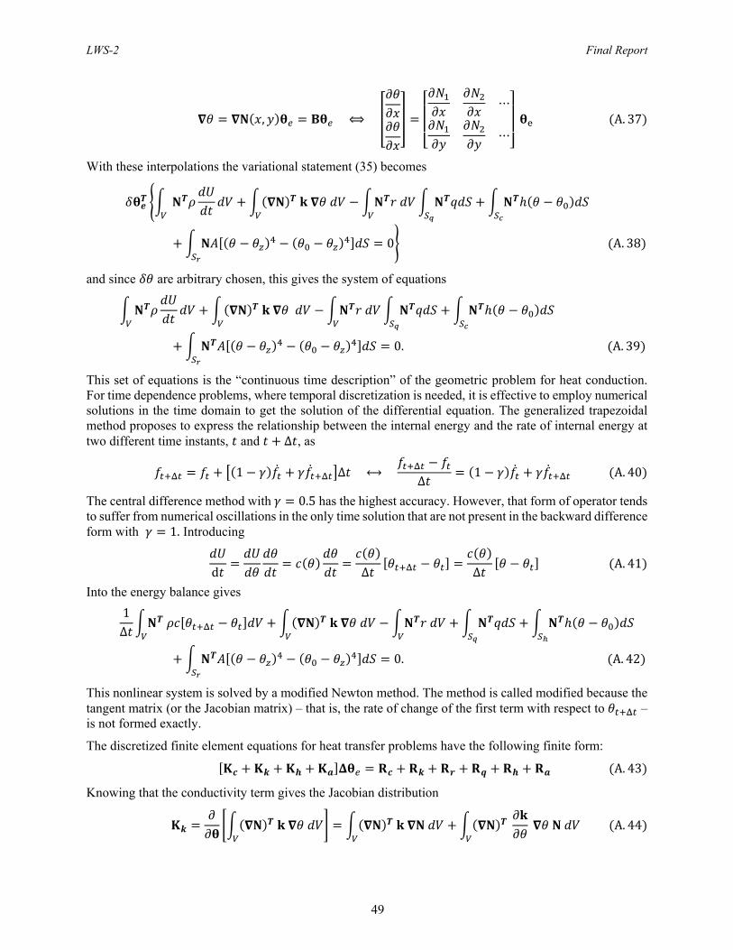
LWS-2 Final Report

49

, ⟺ ⋯

⋯ A. 37

With these interpolations the variational statement (35) becomes

0 A. 38

and since are arbitrary chosen, this gives the system of equations

0. A. 39

This set of equations is the “continuous time description” of the geometric problem for heat conduction. For time dependence problems, where temporal discretization is needed, it is effective to employ numerical solutions in the time domain to get the solution of the differential equation. The generalized trapezoidal method proposes to express the relationship between the internal energy and the rate of internal energy at two different time instants, and Δ , as

1 Δ ⟷ Δ

1 A. 40

The central difference method with 0.5 has the highest accuracy. However, that form of operator tends to suffer from numerical oscillations in the only time solution that are not present in the backward difference form with 1. Introducing

d Δ Δ A. 41

Into the energy balance gives

1Δ

0. A. 42

This nonlinear system is solved by a modified Newton method. The method is called modified because the tangent matrix (or the Jacobian matrix) – that is, the rate of change of the first term with respect to – is not formed exactly.

The discretized finite element equations for heat transfer problems have the following finite form:

A. 43

Knowing that the conductivity term gives the Jacobian distribution

A. 44

LWS-2 Final Report

50

With the Jacobian terms defined as

1Δ

A. 45

A. 46

A. 47

4 A. 48

And the right-hand side residual terms

1Δ

A. 49

A. 50

A. 51

A. 52

A. 53

A. 54

Diffusion

The finite element method for heat conduction can easily adapts itself to the treatment of vector variables for solving a set of several diffusion equations. The same discretization steps of Fourier’s law are repeated but are now addressed to the vector-valued equation of Fick’s law.

A. 55

where is the flux, is the diffusion matrix regrouping the diffusion constants for the material that are diffusing in the specific solvent, and is the concentration gradient in its vectorial form. The diffusion constants of a material are also referred to as ‘diffusion coefficients’ or simply ‘diffusivities’. It is expressed in units of length squared per unit time, such as µm2·hour-1. The negative sign of the right side of the equation indicates that the impurities are flowing in the direction of lower concentration. This is Fick's Second Law, which states that the change in impurity concentrations over time is equal to the change in local diffusion flux

∂∂t

A. 56

or, from Fick's first law,

. 57

LWS-2 Final Report

51

The diffusion equation is the partial differential equation that governs the evolution of the concentration field produced by a given flux. With appropriate boundary and initial conditions, the solution to this equation gives the time and spatial dependence of the concentration. The diffusion equation in the general form is given by

0 A. 58

where is an added source or sink vector term or interior sources corresponding to the rate per unit volume at which diffusing material is created locally due to chemical reactions, heating, cooling, and similar processes.

Using the same Galerkin finite element methodology as for the heat conduction, the weak form that corresponds to the weighted residual formulation for diffusion is:

1Δ

0. A. 59

Implementation in the user element subroutine UEL

The user-element subroutine (UEL) is employed to incorporate the governing equations described in the previous section into the finite element code Abaqus. The UEL subroutine allow to the user to use a maximum number of 20 additional degrees of freedom (DOF's) in addition to the existing degrees of freedom (displacement, temperature, etc.). In this user-designed element, the user must provide the stiffness matrix composed of and as well as the residual vector (right-hand side) as needed in a context of solving the nonlinear system of equations using Newton-Raphson at each iteration. The user-element is written in Fortran language.

The solution is implicitly solved by the incremental method:

applying load in increments/steps: t → t Δt stepping to final time t final in time steps Δt and solving for each step

drop “e” for convenience

We apply the Newton-Raphson method to the following set of nonlinear equations

, ,

, . 60

,

where

, , 0 A. 61

1Δ

0 A. 62

LWS-2 Final Report

52

1Δ

A. 63

Assuming the state is known at the time t, we solve the equation at the time and for the iteration, the Newton-Raphson method gives the solution:

A. 64

The unknowns of the above system of equations are

A. 65

The linear system of equations to solve at each iteration until convergence is

with A. 66

where the unsymmetric stiffness matrix of the system is

0

A. 67

For example, using the stress update algorithm, the stiffness matrix term is defined by

, , A. 68

where

A. 69

is the Jacobian of the constitutive law, also called the tangent consistent matrix. The two terms that must be defined in the user elements subroutine UEL are the stiffness matrix and the right hand side .

, ,

LWS-2 Final Report

53

, , A. 70

, ,

, , . 71

The Jacobian term for the heat transfer equation is defined by

A. 72

with

1Δ

A. 73

A. 74

A. 75

4 A. 76

Finally for the Jacobian terms in the diffusion equation.

A. 77

with

1Δ

A. 78

A. 79

A. 80

A. 82

If the volumetric heat generation is caused by mechanical working and diffusion mechanisms of the material, the following Jacobian terms must defined

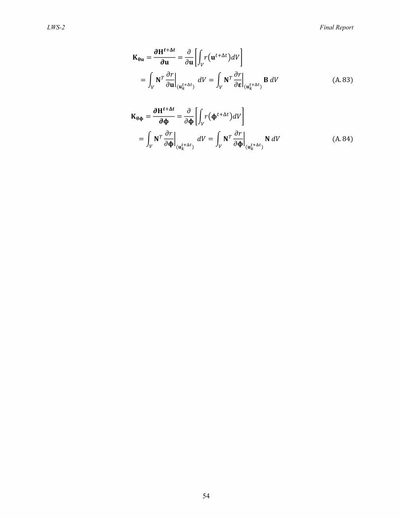
LWS-2 Final Report

54

A. 83

A. 84

LWS-2 Final Report

55

Applendix B

Implementation in UEL Subroutine

A. Equilibrium 1. Initialization of material stiffness matrix DDSDDE and Element Stiffness Matrix AMATRX for

LFLAGS(3)=4

and B. 1

2. Initialization of Stiffness Matrix AMATRX and Right-Hand Side RHS

and B. 2

3. Calculation of current coordinates as function of initial coordinates and displacements

B. 3

4. Loop over integrations points

a. Evaluate shape functions and derivatives

, and , in2D B. 4

, , and , , in3D B. 5

b. Compute coordinates at the integration points

For small displacement analysis, i.e. LFLAGS(2) = 0, use For large displacement analysis, i.e. LFLAGS(2) = 1, use

, and , in2D B. 6

, , , , , and , , in3D B. 7

In matrix form, we have

0

00

0 ⋯0

0 ⋮in2D B. 8

LWS-2 Final Report

56

0 0

0 00 0

0 00 00 0

⋯0 0

0 00 0 ⋮

in3D B. 9

c. Compute Jacobian , its determinant det , and its inverse

in2D B. 10

in3D B. 11

d. Form -Matrix

If the inverse of the Jacobian matrix can be determined, the followings equations

in2D B. 11

in3D B. 12

can be solved for the partial derivatives of the interpolation functions with respect to the global coordinates to obtain

in2D B. 13

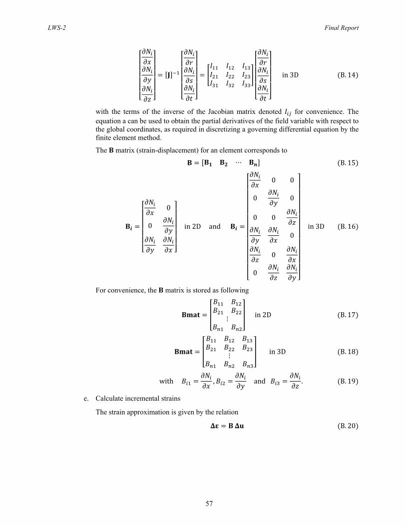
LWS-2 Final Report

57

in3D B. 14

with the terms of the inverse of the Jacobian matrix denoted for convenience. The equation a can be used to obtain the partial derivatives of the field variable with respect to the global coordinates, as required in discretizing a governing differential equation by the finite element method.

The matrix (strain-displacement) for an element corresponds to

⋯ B. 15

0

0 in2Dand

0 0

0 0

0 0

0

0

0

in3D B. 16

For convenience, the matrix is stored as following

⋮ in2D B. 17

⋮ in3D B. 18

with , and . B. 19

e. Calculate incremental strains

The strain approximation is given by the relation

B. 20

LWS-2 Final Report

58

ΔΔΔ

0

0 ⋯

0

0

ΔΔ⋮

ΔΔ

in2D B. 21

ΔΔΔΔΔΔ

0 0

0 0

0 0

0

0

0

⋯

0 0

0 0

0 0

0

0

0

ΔΔ

Δ⋮

ΔΔΔ

in3D B. 22

f. Calculate deformation gradients

The fundamental deformation gradient tensor F is interpolated over an element by differentiating the equation

u N u B. 22

with respect to the initial coordinates to give an explicit matrix form

in2D B. 23

in3D B. 24

with Δ and B. 25

g. Material routine for computing stresses and the material stiffness / using a user material subroutine UMAT.

h. Store strains , stresses , and other internal state variables in array SVARS i. Form stiffness matrix at internal point contribution

The stiffness matrix in the user element subroutine correspond to

B. 26

which has the following form

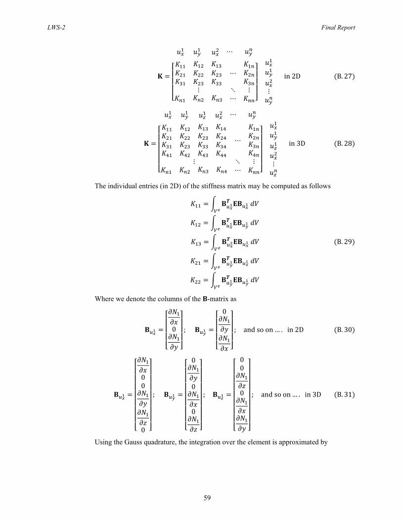
LWS-2 Final Report

59

⋯

⋯

⋮ ⋱ ⋮⋯

⋮

in2D B. 27

⋯

⋯

⋮ ⋱ ⋮⋯

⋮

in3D B. 28

The individual entries (in 2D) of the stiffness matrix may be computed as follows

B. 29

Where we denote the columns of the -matrix as

0 ;

0

; andsoon… .in2D B. 30

00

0

;

0

0

0

;

00

0 ; andsoon… .in3D B. 31

Using the Gauss quadrature, the integration over the element is approximated by

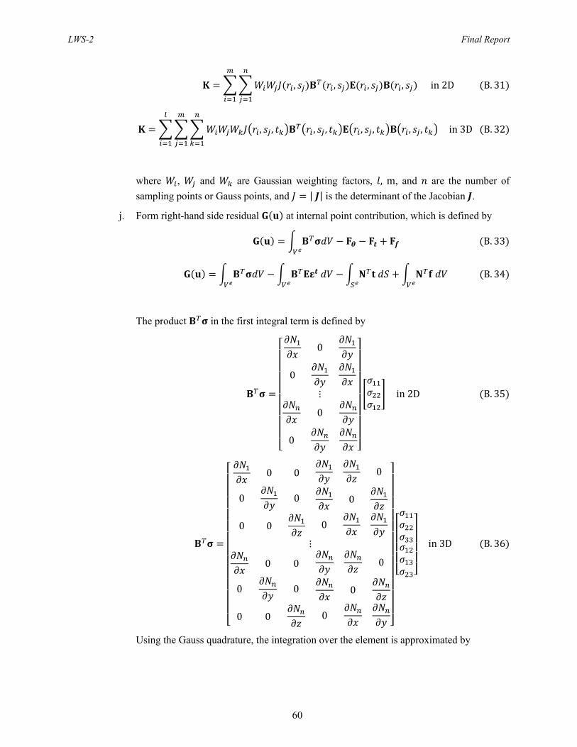
LWS-2 Final Report

60

, , , , in2D B. 31

, , , , , , , , in3D B. 32

where , and are Gaussian weighting factors, , m, and are the number of

sampling points or Gauss points, and | | is the determinant of the Jacobian .

j. Form right-hand side residual at internal point contribution, which is defined by

B. 33

B. 34

The product in the first integral term is defined by

0

0

⋮

0

0

in2D B. 35

0 0

0 0

0 0

0

0

0

⋮

0 0

0 0

0 0

0

0

0

in3D B. 36

Using the Gauss quadrature, the integration over the element is approximated by

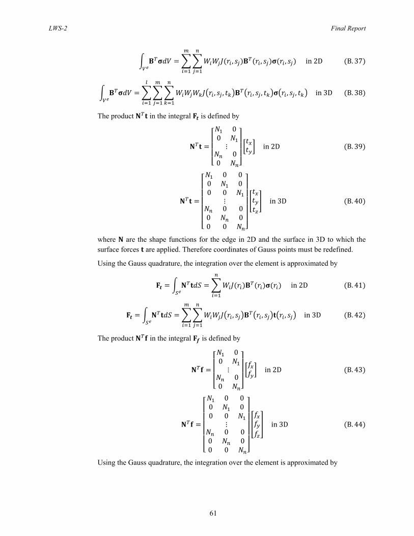
LWS-2 Final Report

61

, , , in2D B. 37

, , , , , , in3D B. 38

The product in the integral is defined by

00⋮0

0

in2D B. 39

0 00 00 0

⋮0 0

0 00 0

in3D B. 40

where are the shape functions for the edge in 2D and the surface in 3D to which the surface forces are applied. Therefore coordinates of Gauss points must be redefined.

Using the Gauss quadrature, the integration over the element is approximated by

in2D B. 41

, , , in3D B. 42

The product in the integral is defined by

00⋮0

0

in2D B. 43

0 00 00 0

⋮0 0

0 00 0

in3D B. 44

Using the Gauss quadrature, the integration over the element is approximated by

LWS-2 Final Report

62

, , , in2D B. 45

, , , , , , in3D B. 46

In case of thermal expansion, the product n the integral is defined by

0

0

⋮

0

0

Δ1 2

110in2D B. 47

0 0

0 0

0 0

0

0

0

⋮

0 0

0 0

0 0

0

0

0

Δ1 2

111000

in3D B. 48

Using the Gauss quadrature, the integration over the element is approximated by

, , , in2D B. 49

, , , , , , in3D B. 50

In case of (steady state or transient) fully coupled thermal-stress analysis (LFLAGS(1)=71,72,73), if the stresses are temperature dependent, the following Jacobian term must be determined

Δ

1 2 B. 51

with

LWS-2 Final Report

63

0

0

⋮

0

0

⋯ in2D B. 52

Δ1 2

Δ

1 2

0

0

⋮

0

0

110

⋯ in2D B. 53

0 0

0 0

0 0

0

0

0

⋮

0 0

0 0

0 0

0

0

0

⋯ in3D B. 54

Δ1 2

Δ

1 2

0 0

0 0

0 0

0

0

0

⋮

0 0

0 0

0 0

0

0

0

111000

⋯ in3D B. 55

LWS-2 Final Report

64

Using the Gauss quadrature, the integration over the element is approximated by

, , , , in2D B. 56

, , , , , , , , in3D B. 57

B. Heat Transfer

1. Initialization of Element Stiffness Matrix AMATRX and the right-hand side for LFLAGS(1)=33

and B. 58

2. Determination of the Gauss points locations , in 2D and , , in 3D

3. Determination of the Gauss points locations , in 2D and , , in 3D

4. Loop over integrations points

a. Evaluate shape functions and derivatives

, and , in2D B. 59

, , and , , in3D B. 60

b. Compute Jacobian , its determinant det , and its inverse

in2D B. 61

in3D B. 62

c. Calculate the derivative of shape functions with respect to global coordinates

If the inverse of the Jacobian matrix can be determined, the followings equations

LWS-2 Final Report

65

in2D B. 63

in3D B. 64

can be solved for the partial derivatives of the interpolation functions with respect to the global coordinates to obtain

in2D B. 65

in3D B. 66

with the terms of the inverse of the Jacobian matrix denoted for convenience. The equation a can be used to obtain the partial derivatives of the field variable with respect to the global coordinates, as required in discretizing a governing differential equation by the finite element method.

d. Compute temperature and its derivatives with respect to the global coordinates:

, ,in2D B. 67

, , in3D B. 68

and its derivatives / , / and / with respect to global coordinates

, , in2D B. 69

, , , , , , , in3D B. 70

e. Determine the temperature dependence of thermal conductivity

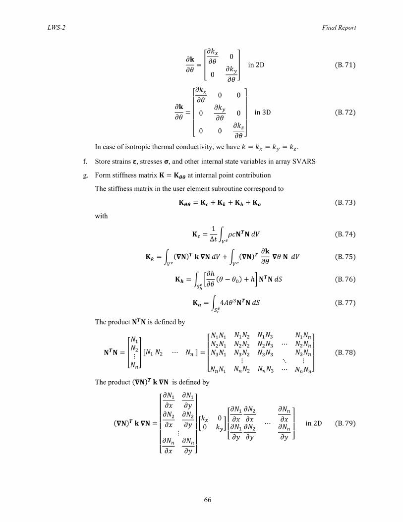
LWS-2 Final Report

66

0

0in2D B. 71

0 0

0 0

0 0

in3D B. 72

In case of isotropic thermal conductivity, we have .

f. Store strains , stresses , and other internal state variables in array SVARS

g. Form stiffness matrix at internal point contribution

The stiffness matrix in the user element subroutine correspond to

B. 73

with

1Δ

B. 74

B. 75

B. 76

4 B. 77

The product is defined by

⋮ ⋯

⋯

⋮ ⋱ ⋮⋯

B. 78

The product is defined by

⋮

00 ⋯ in2D B. 79

LWS-2 Final Report

67

⋮

0 00 00 0

⋯ in3D B. 80

The product is defined by

⋮

0

0 ⋯ in2D B. 81

⋮

0 0

0 0

0 0

⋯ in3D B. 82

Where is defined by

⋯ ⋮ in2D B. 83

⋯ ⋮ in3D B. 84

Using the Gauss quadrature, the integration over the 2D element is approximated by

1Δ

, , , B. 85

, , ,

LWS-2 Final Report

68

, , , , B. 86

on B. 87

4 on B. 88

And over the 3D element

1Δ

, , , , , , B. 89

, , , , , ,

, , , , , , , , B. 90

, , , , on B. 91

, 4 , , on B. 92

where , and are Gaussian weighting factors, , m, and are the number of

sampling points or Gauss points, and | | is the determinant of the Jacobian .

h. Form right-hand side residual at internal point contribution, which is defined by

B. 93

1Δ

B. 94

Using the Gauss quadrature, the integration of over the element is approximated by

1Δ

, , in2D B. 95

1Δ

, , , , , , in3D B. 96

LWS-2 Final Report

69

The product in the second integral term is defined by

⋮

00 in2D B. 97

⋮

0 00 00 0

in3D B. 98

Using the Gauss quadrature, the integration of over the element is approximated by

1Δ

, , in2D B. 99

, , , , , , in3D B. 100

where are the shape functions for the edge in 2D and the surface in 3D to which the surface forces are applied. Therefore coordinates of Gauss points must be redefined.

1Δ

, , in2D B. 101

, , , , , , in3D B. 102

Using the Gauss quadrature, the integration over the element of the three other integral terms is approximated by

in2D B. 103

, , , in3D B. 104

in2D B. 105

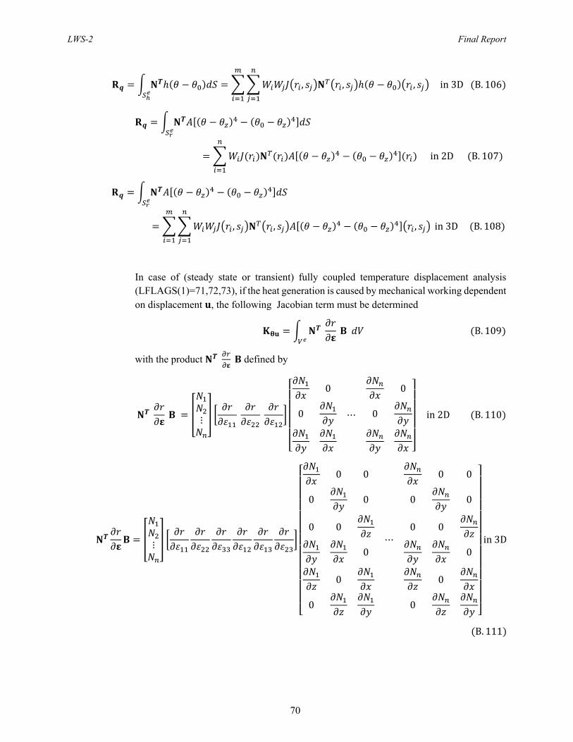
LWS-2 Final Report

70

, , , in3D B. 106

in2D B. 107

, , , in3D B. 108

In case of (steady state or transient) fully coupled temperature displacement analysis (LFLAGS(1)=71,72,73), if the heat generation is caused by mechanical working dependent on displacement , the following Jacobian term must be determined

B. 109

with the product defined by

⋮

0

0 ⋯

0

0 in2D B. 110

⋮

0 0

0 0

0 0

0

0

0

⋯

0 0

0 0

0 0

0

0

0

in3D

B. 111

LWS-2 Final Report

71

In case of (steady state or transient) fully coupled thermal-diffusion analysis (LFLAGS(1)=71,72,73), if the conductivity is dependent on concentration variables , the following Jacobian term must be determined

B. 112

with the product defined by

⋮

0

0 ⋯ in2D B. 113

⋮

0 0

0 0

0 0

⋯ in3D B. 114

Using the Gauss quadrature, the integration over the element is approximated by

, , , , in2D B. 115

, , , , , , , , in3D B. 116

C. Diffusion

The discretization of diffusion equations is similar to that of heat transfer, therefore the same steps are repeated to solve the diffusion equations. The diffusion equations represents a set of several diffusion equations to find the vector of concentration variables . For example, if is a vector of three different concentration variables , and , it is discretized by

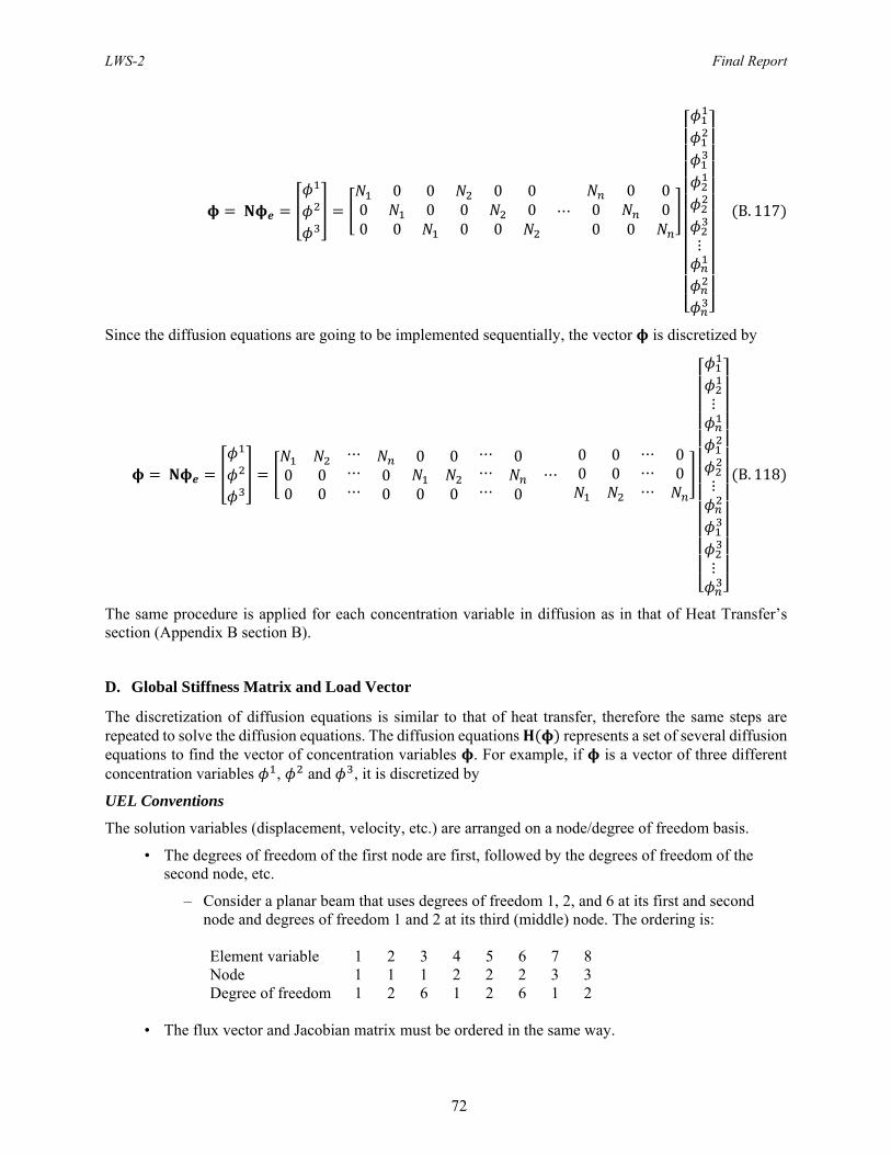
LWS-2 Final Report

72

0 0

0 00 0

0 00 00 0

⋯0 0

0 00 0

⋮

B. 117

Since the diffusion equations are going to be implemented sequentially, the vector is discretized by

00

00

⋯⋯⋯

00

0

0

0

0

⋯⋯⋯

0

0⋯

00

00

⋯⋯⋯

00

⋮

⋮

⋮

B. 118

The same procedure is applied for each concentration variable in diffusion as in that of Heat Transfer’s section (Appendix B section B).

D. Global Stiffness Matrix and Load Vector

The discretization of diffusion equations is similar to that of heat transfer, therefore the same steps are repeated to solve the diffusion equations. The diffusion equations represents a set of several diffusion equations to find the vector of concentration variables . For example, if is a vector of three different concentration variables , and , it is discretized by

UEL Conventions

The solution variables (displacement, velocity, etc.) are arranged on a node/degree of freedom basis.

• The degrees of freedom of the first node are first, followed by the degrees of freedom of the second node, etc.

– Consider a planar beam that uses degrees of freedom 1, 2, and 6 at its first and second node and degrees of freedom 1 and 2 at its third (middle) node. The ordering is:

Element variable 1 2 3 4 5 6 7 8 Node 1 1 1 2 2 2 3 3 Degree of freedom 1 2 6 1 2 6 1 2

• The flux vector and Jacobian matrix must be ordered in the same way.

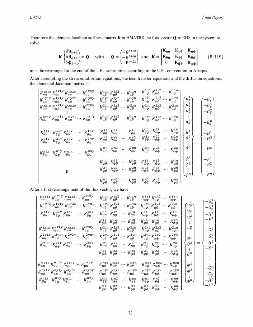
LWS-2 Final Report

73

Therefore the element Jacobian stiffness matrix AMATRX the flux vector RHS in the system to solve

with and0

B. 119

must be rearranged at the end of the UEL subroutine according to the UEL convention in Abaqus.

After assembling the stress equilibrium equations, the heat transfer equations and the diffusion equations, the elemental Jacobian matrix is

⋯

⋯

⋯⋮

⋯

⋯

⋯

⋯⋮

⋯

⋯

⋯

⋯⋮

⋯

⋯

⋯⋮

⋯

⋯ ⋯

⋮ ⋯

⋯

⋯⋮

⋯

0

⋯

⋯⋮

⋯

⋯

⋯⋮

⋯

⋮

⋮

⋮

⋮

⋮

⋮

After a first rearrangement of the flux vector, we have

⋯ ⋯ ⋯

⋯ ⋯ ⋯

⋯ ⋯ ⋯

⋯ ⋯

⋯ ⋯ ⋯

⋯ ⋯ ⋯

⋯ ⋯ ⋯

⋯ ⋯

⋮ ⋯ ⋯ ⋯

⋯ ⋯ ⋯

⋯ ⋯ ⋯

⋯ ⋯

⋮

⋮

⋮

⋮

LWS-2 Final Report

74

After a second rearrangement of the displacement vector, we obtain

⋯

⋯

⋯

⋯

⋯

⋯

⋯

⋯

⋮

⋯

⋯

⋯

⋯

⋮ ⋮