Multiscale boundary conditions in crystalline solids...

International Journal of Solids and Structures 43 (2006) 6359–6379

www.elsevier.com/locate/ijsolstr

Multiscale boundary conditions in crystalline solids:Theory and application to nanoindentation

E.G. Karpov a,*, H. Yu a, H.S. Park b, Wing Kam Liu a, Q. Jane Wang a, D. Qian c

a Department of Mechanical Engineering, Northwestern University, 2145 Sheridan Road, Evanston, IL 60208, United Statesb Department of Civil and Environmental Engineering, Vanderbilt University, Nashville, TN 37235, United States

c Department of Mechanical, Industrial and Nuclear Engineering, University of Cincinnati, P.O. Box 210072,

Cincinnati, OH 45221, United States

Received 31 May 2005; received in revised form 24 August 2005Available online 29 November 2005

Abstract

This paper presents a systematic approach to treating the interfaces between the localized (fine grain) and peripheral(coarse grain) domains in atomic scale simulations of crystalline solids. Based on Fourier analysis of regular lattices struc-tures, this approach allows elimination of unnecessary atomic degrees of freedom over the coarse grain, without involvingan explicit continuum model for the latter. The mathematical formulation involves compact convolution operators thatrelate displacements of the interface atoms and the adjacent atoms on the coarse grain. These operators are defined bygeometry of the lattice structure, and interatomic potentials. Application and performance are illustrated on quasistaticnanoindentation simulations with a crystalline gold substrate. Complete atomistic resolution on the coarse grain is alter-natively employed to give the benchmark solutions. The results are found to match well for the multiscale and the fullatomistic simulations.� 2005 Elsevier Ltd. All rights reserved.

Keywords: Boundary conditions; Multiscale simulation; Molecular dynamics; Crystal structure; Nanoindentation

1. Introduction

Over the past few decades, continuum methods have dominated materials modeling research. Thisapproach of predicting material deformation and failure by implicitly averaging atomic scale mechanicsand defect evolution over time and space, however, is valid only for sufficiently large systems that include asubstantial number of inhomogeneities. As a result, numerous experimental observations of material behaviorcannot be readily explained within the continuum mechanics framework: dislocation patterns in fatigue andcreep, surface roughening and crack nucleation in fatigue, the inherent inhomogeneity of plastic deformation,the statistical nature of brittle failure, plastic flow localization in shear bands, and the effects of size, geometry,

0020-7683/$ - see front matter � 2005 Elsevier Ltd. All rights reserved.

doi:10.1016/j.ijsolstr.2005.10.003

* Corresponding author. Tel.: +1 847 491 3915.E-mail address: [email protected] (E.G. Karpov).

mailto:[email protected]

6360 E.G. Karpov et al. / International Journal of Solids and Structures 43 (2006) 6359–6379

and stress state on yield properties. Thus, there is a considerable effort to find fundamental descriptions ofstrength and failure properties of nanoscale materials, taking into account their atomic structures. The useof molecular dynamics/quasistatic atomistic simulations has provided useful information on material behaviorat the nanoscale. However, typical atomistic simulations are still restricted to very small systems consisting ofseveral million atoms or less and timescales on the order of picoseconds. Thus, even for nanoscale structuresand materials, atomistic modeling would be computationally prohibitive. The limitations of atomistic simula-tions and continuum mechanics, along with practical needs arising from the heterogeneous nature of engineer-ing materials, have motivated the research on multiscale simulation methods that bridge atomistic simulationsand continuum modeling; examples include the works by Curtin and Miller (2003), Liu et al. (2004), Shilkrotet al. (2004), Broughton et al. (1999), Abraham et al. (1998), Rudd and Broughton (1998, 2000), Tadmor et al.(1996), Shenoy et al. (1998), Ortiz et al. (2001), Deymier and Vasseur (2002), Wagner and Liu (2003) and Parket al. (2005b,c). In order to make computations tractable, the multiscale models generally make use of acoarse-fine grain decomposition for the physical domain under analysis. An atomistic simulation method isused in a small subregion, the fine grain, where it is crucial to capture the individual atomistic behavior accu-rately. A continuum simulation is used in a larger peripheral region, the coarse grain, where the deformation isconsidered to be homogeneous and smooth; the macroscopic material behavior and properties are mainlydetermined by the collective atomic motion. Since the continuum region is usually chosen to be much largerthan the atomistic region, the overall domain of interest can be considerably large. A purely atomistic solutionis normally not affordable on this domain, though the multiscale solution would presumably provide thedetailed atomistic information only when and where it is necessary.

The key issue is then the coupling between the coarse and fine scales. An approximation is necessary alongthe fine-coarse grain interface, due to the fundamental incompatibility of the atomistic and continuum descrip-tions (e.g., Deymier and Vasseur, 2002). This incompatibility is imposed by mismatch of the dispersion char-acteristics of the continuous and discrete media in dynamic simulations, and by the non-local character of theatomic interaction in dynamic and quasistatic simulations. Typically, the concurrent coupling involves theidea of a ‘‘handshake’’ or ‘‘pad’’ region, e.g., Curtin and Miller (2003), Liu et al. (2004), Shilkrot et al.(2004), Broughton et al. (1999), Abraham et al. (1998), Rudd and Broughton (1998, 2000), Tadmor et al.(1996), Shenoy et al. (1998) and Ortiz et al., 2001, where pseudoatoms are available on the continuum partof the interface and share the physical space with finite elements, as shown in Fig. 1. At the front end ofthe continuum interface, the finite elements have to be scaled down to the atomic bond lengths. The purposeof the handshake region is to assure smoother coupling between the atomistic and continuum regimes. Thegroup of pseudoatoms serves to eliminate the non-physical surface in the atomistic lattice structure, so that

Fig. 1. Structure of the transition region in coupled atomistic/continuum simulations. Positions of pseudoatoms in the handshake area areinterpolated with finite element shape functions.

E.G. Karpov et al. / International Journal of Solids and Structures 43 (2006) 6359–6379 6361

the real atoms along the interface have a full set of interactive neighbors in the continuum domain. In dynamicsimulations, the handshake also serves as a damper/absorbent to reduce the spurious reflection of high fre-quency phonons that cannot pass into the coarse scale domain. However, this reflection can be eliminated onlypartially by a reasonably sized handshake domain. Besides, introduction of a non-physical handshake regionleads to the three other concerns in both dynamic and quasistatic modelling. The first is double counting of thestrain energy in the handshake region by the atomistic and continuum models. The second is ill-conditioning ofthe finite element stiffness matrices, due to the need in atomic length scale refinement of the finite element meshfor the handshake region. Indeed, an extremely fine mesh is required in order to provide accurate positions ofthe pseudoatoms, since they are found by interpolating the finite element nodal positions (Curtin and Miller,2003). Note that the FE interpolation procedure can be written symbolically,

u1 ¼ Nd ð1Þ

where u1 are displacements of the pseudoatoms interacting with the interface atoms, d are finite element nodaldisplacements, and the columns of the rectangular matrix N give a set of interpolation basis vectors, computedby utilizing the FE shape functions. And the third concern is related to the need in a non-local continuummodel for the small length scales that are typical for the handshake region.

An alternative methodology has been proposed recently for dynamic simulations (Karpov et al., 2005,2004; Park et al., 2005a), where positions of actual next-to-interface atoms from the coarse grain are computedby means of a functional operator over displacements of the interfacial atoms. This operator essentially relatesthe displacements of coarse grain atoms interacting with the interface, u1, and the interface atomic displace-ments, u0, as u1 = H{u0} at all times. Here and further, all atomic displacements are implied about equilibriumpositions in the ideal crystal lattice. The derivation of the interface operator H is a straightforward semi-ana-lytical procedure based on the Fourier analysis of periodic lattice structures (Karpov et al., 2002; Karpovet al., 2003; Ryvkin et al., 1999), which provides the required solution at the intrinsic atomistic level. For linearcoarse grains with regular crystalline interfaces, this operator was shown to act as a convolution integral witha compact and spatially invariant kernel function of time. However, this model is only applicable to the case ofinfinite coarse grains. Here, infiniteness of the coarse grain is understood in the sense that the progressivewaves caused by the peripheral boundary conditions do not reach the fine-coarse grain interface during theprescribed simulation time. In other words, this approach is applicable to problems with only inner (fine grain)excitations of the time-dependent deformation; examples are heat transfer in contact problems, dynamic nan-oindentation and deposition problems.

One interesting approach to atomistic-continuum coupling is the bridging scale method (Wagner and Liu,2003; Park et al., 2005b,c). This method employs the dynamic multiscale boundary conditions to give a forcef1!0 exerted on the interface atoms from the side of all the coarse grain atoms eliminated from the explicitconsideration. In principle, this force is computed based on the displacements u0 and u1, where u1 = H{u0}.The force f1!0 is also called the lattice impedance force, because it represents the dynamic response charac-teristics of a crystal lattice along a fine/coarse grain interface. The original form of this method was presentedfor the case of short range potentials, where it did not require a handshake domain. However, the long-rangeatomic forces may still impose a small overlapping domain, and therefore double counting of the strainenergy, within the effective range of these forces.

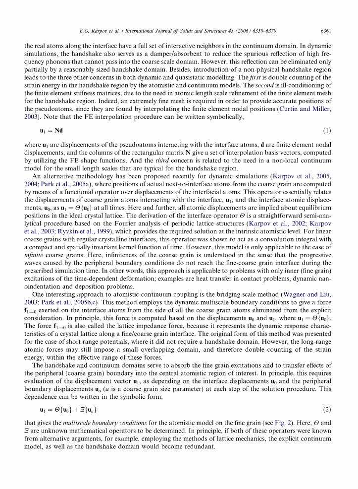
The handshake and continuum domains serve to absorb the fine grain excitations and to transfer effects ofthe peripheral (coarse grain) boundary into the central atomistic region of interest. In principle, this requiresevaluation of the displacement vector u1, as depending on the interface displacements u0 and the peripheralboundary displacements ua (a is a coarse grain size parameter) at each step of the solution procedure. Thisdependence can be written in the symbolic form,

u1 ¼ Hfu0g þ Nfuag ð2Þ

that gives the multiscale boundary conditions for the atomistic model on the fine grain (see Fig. 2). Here, H andN are unknown mathematical operators to be determined. In principle, if both of these operators were knownfrom alternative arguments, for example, employing the methods of lattice mechanics, the explicit continuummodel, as well as the handshake domain would become redundant.

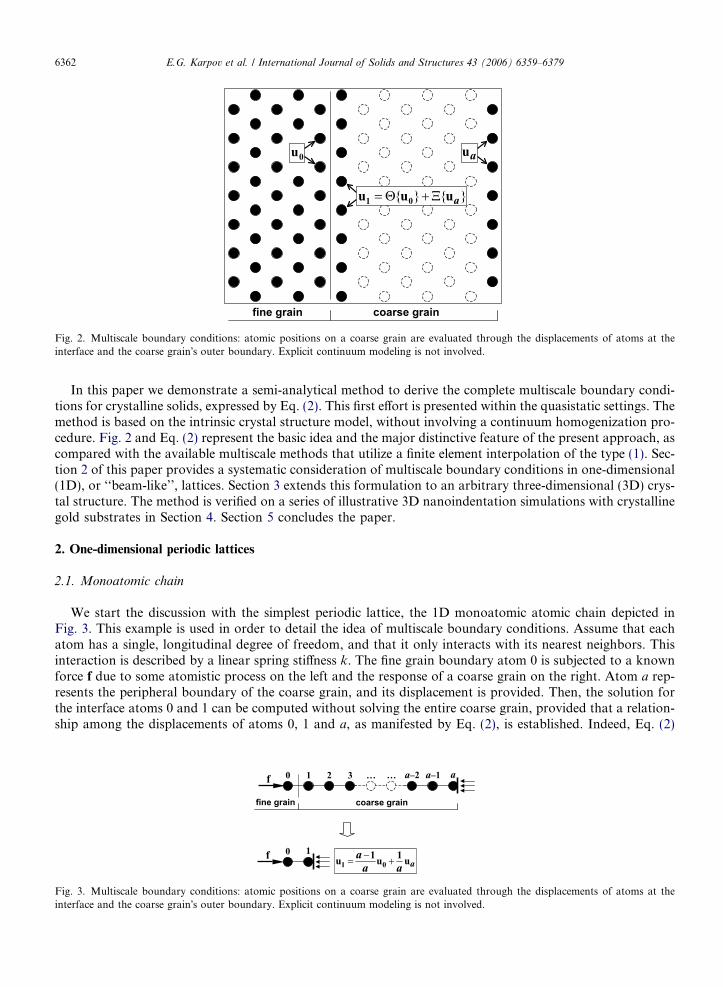
Fig. 2. Multiscale boundary conditions: atomic positions on a coarse grain are evaluated through the displacements of atoms at theinterface and the coarse grain�s outer boundary. Explicit continuum modeling is not involved.


In this paper we demonstrate a semi-analytical method to derive the complete multiscale boundary condi-tions for crystalline solids, expressed by Eq. (2). This first effort is presented within the quasistatic settings. Themethod is based on the intrinsic crystal structure model, without involving a continuum homogenization pro-cedure. Fig. 2 and Eq. (2) represent the basic idea and the major distinctive feature of the present approach, ascompared with the available multiscale methods that utilize a finite element interpolation of the type (1). Sec-tion 2 of this paper provides a systematic consideration of multiscale boundary conditions in one-dimensional(1D), or ‘‘beam-like’’, lattices. Section 3 extends this formulation to an arbitrary three-dimensional (3D) crys-tal structure. The method is verified on a series of illustrative 3D nanoindentation simulations with crystallinegold substrates in Section 4. Section 5 concludes the paper.

2. One-dimensional periodic lattices

2.1. Monoatomic chain

We start the discussion with the simplest periodic lattice, the 1D monoatomic atomic chain depicted inFig. 3. This example is used in order to detail the idea of multiscale boundary conditions. Assume that eachatom has a single, longitudinal degree of freedom, and that it only interacts with its nearest neighbors. Thisinteraction is described by a linear spring stiffness k. The fine grain boundary atom 0 is subjected to a knownforce f due to some atomistic process on the left and the response of a coarse grain on the right. Atom a rep-resents the peripheral boundary of the coarse grain, and its displacement is provided. Then, the solution forthe interface atoms 0 and 1 can be computed without solving the entire coarse grain, provided that a relation-ship among the displacements of atoms 0, 1 and a, as manifested by Eq. (2), is established. Indeed, Eq. (2)

Fig. 3. Multiscale boundary conditions: atomic positions on a coarse grain are evaluated through the displacements of atoms at theinterface and the coarse grain�s outer boundary. Explicit continuum modeling is not involved.


solved simultaneously with the force/displacement relationship, k(u1 � u0) = �f, provides unique displace-ments u0 and u1. Eq. (2) contains two mathematical operators H and N, whose form depends on the latticeproperties and the coarse scale size parameter a. Technically, the objective of this paper is to provide a generalapproach to deriving these operators for arbitrary periodic lattice structures.

The periodicity of the monoatomic chain implies a uniform character of the equilibrium deformation understatic end loadings, so that

u1 ¼a� 1

au0 þ

1

aua ð3Þ

for arbitrary displacements u0 and ua. This formula can be obtained based on elementary arguments: thesought displacement u1 is given by a first order interpolation polynomial, satisfying the sample values u0

and ua at x = 0 and x = a, and then evaluated at x = 1.In principle, Eq. (3) represents the multiscale boundary condition for the monoatomic 1D chain. It can be

regarded as an additional equation for the boundary degree of freedom, u1, and solved simultaneously withgeneral molecular mechanics equations for the fine grain degrees of freedom, i.e., displacements un at n < 1.The resultant solution will automatically incorporate the effect of the peripheral degrees of freedom, un atn = 1,2, . . . ,a.

We emphasize that atom 1 will then serve as the actual boundary of the computational domain, though itsdisplacement must be updated at each step of the molecular mechanics energy minimization procedure. Thedisplacement of the boundary atom 1 will be determined by both the peripheral and local effects; we will referto such an atom or group of atoms (in two- and three-dimensional applications) as the multiscale boundary.For more complicated periodic structures, the multiscale boundary conditions can be evaluated on the basis ofdiscrete Fourier transform, as discussed in below Sections 2.2 and 3.

2.2. Arbitrary beam-like lattices

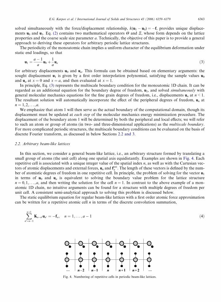
In this section, we consider a general beam-like lattice, i.e., an arbitrary structure formed by translating asmall group of atoms (the unit cell) along one spatial axis equidistantly. Examples are shown in Fig. 4. Eachrepetitive cell is associated with a unique integer value of the spatial index n, as well as with the Cartesian vec-tors of atomic displacements and external forces, un and fext

n . The length of these vectors is defined by the num-ber of atomistic degrees of freedom in one repetitive cell. In principle, the problem of solving for the vector u1

in terms of u0 and ua is equivalent to solving the boundary value problem for the lattice structuren = 0,1, . . . ,a, and then writing the solution for the cell n = 1. In contrast to the above example of a mon-atomic 1D chain, no intuitive arguments can be found for a structure with multiple degrees of freedom perunit cell. A consistent semi-analytical approach to solving this problem is discussed below.

The static equilibrium equation for regular beam-like lattices with a first order atomic force approximationcan be written for a repetitive atomic cell n in terms of the discrete convolution summation,

Xnþ1

Kn�n0un0 ¼ �fn; n ¼ 1; . . . ; a� 1 ð4Þ
n0¼n�1
Fig. 4. Numbering of repetitive cells in periodic beam-like lattices.


where u and f are s-component vectors of displacements and external forces in the corresponding unit cells, s isthe number of degrees of freedom in one cell; u0 and ua are viewed as the boundary conditions. Since the coarsegrain is free of in-domain external loads, the force vector for this equation is given by

fn ¼ dn;0f0 þ dn;afa; n ¼ 0; 1; . . . ; a ð5Þ

where d is the Kronecker delta, and f0, fa are unknown boundary forces. Eq. (4) assumes that each cell n inter-acts only with two adjacent cells n � 1 and n + 1. The K-matrices in (4) represent elastic properties of the lat-tice structure. They can be expressed through the potential energy of the lattice, U, utilized in terms of thedisplacements about equilibrium positions

Kn�n0 ¼ �o2UðuÞoun oun0

��u¼0

ð6Þ

Obviously, the matrices Kn�n0 are invariant with respect to n in a regular lattice; therefore this procedure has tobe accomplished only once—for an arbitrary cell n to yield three non-trivial matrices K�1, K0 and K1.

The governing equation (4) gives a coupled system of linear finite difference equations, which can be solvedselectively for u1 by adapting the discrete Fourier transform method (e.g., Karpov et al., 2002, 2003). The dis-crete Fourier transform of a sequence of numbers, vectors, or matrices gn is defined as the sum over all non-trivial elements of this sequence,

gðpÞ ¼Fn!pfgng ¼Xnmax

n¼nmin

gne�ipn; p 2 ½�p; p� ð7Þ

Here, the hatted notation g stands for the Fourier images, nmin and nmax are the minimal and maximal valuesof the integer index n for a given sequence, and the calligraphic symbols F denotes the Fourier transformoperator. The inversion formula is given by

gn ¼F�1p!nfgðpÞg ¼

1

2N

XN�1=2

vp¼1=2�N

gpvp

N

� �eipvpn=N ð8Þ

Here, the semi-integer summation index vp is utilized, and the value 2N gives the domain�s size, or length of thesequence gn : nmax � nmin + 1. For the present problem, we have 2N = a + 1 that gives a lateral size of thecoarse grain in unit cells. Derivation of the formula (8) and the relevant discussion are provided in AppendixA. For the purpose of further discussion, we recall two properties of the DFT: the convolution and shift the-orems (proves are provided in Appendix A),

FX

n0fn�n0gn0

( )¼ f ðpÞgðpÞ ð9Þ

Ffgnþhg ¼ gðpÞeihp; ð10Þ

where h is integer. Applying the discrete Fourier transform (7) over Eq. (4), and taking into account the con-volution theorem (9), we obtain

KðpÞuðpÞ ¼ �fðpÞ ð11Þ

Hence, the Fourier domain solution reads

uðpÞ ¼ �K�1ðpÞfðpÞ ð12Þ

Next we apply the inverse DFT with the convolution theorem to (12), and utilize the force vector (5). Thisgives the real-space displacement vector u in terms of the n-parametric s · s matrix G called the lattice Green�sfunction (Karpov et al., 2002, 2003)


un ¼Xa

n0¼0

Gn�n0 fn0 ¼ Gnf0 þGn�afa; n ¼ 0; 1; . . . ; a ð13Þ

Gn ¼1

2N

XN�1=2

vp¼1=2�N

Gpvp

N

� �eipvpn=N ; N ¼ aþ 1

2ð14Þ

Here,

GðpÞ ¼ �K�1ðpÞ � �ðFfKngÞ�1 ¼ � K�1eip þ K0 þ K1e�ip

� ��1 ð15Þ

Next we write the displacement vector, expressed by Eq. (13), at n = 0, n = 1 and n = a,

u0 ¼ G0f0 þG�afa

u1 ¼ G1f0 þG1�afa

ua ¼ Gaf0 þG0fa

ð16Þ

and express the unknown force vectors f0 and fa in terms of u0 and ua using the first and the third equations of(16)

f0

fa

� �¼

G0 G�a

Ga G0

� ��1u0

ua

� �ð17Þ

Finally, we employ the external force vectors (17) in the second equation of (16) to obtain the general 1D mul-tiscale boundary condition in the matrix form

u1 ¼ Hu0 þ Nua ð18Þ

H Nð Þ ¼ G1 G1�að ÞG0 G�a

Ga G0

� ��1

ð19Þ

Thus, the sought operators of multiscale boundary conditions for beam-like lattices are s · s square matricesdefined solely by the interatomic potential and the coarse scale parameter a. We note that the matrix Gn, Eq.(14), is evaluated only at n = �a, 1 � a, 0, and 1. The cost of such an inverse DFT procedure is only �N1, sothat relatively large linear dimensions of the coarse scale domain will be accessible with the usage of moderncomputers (up to a � 104, . . . , 107, depending on complexity of the unit cell).

This formulation can be verified on the 1D lattice example discussed in Section 2.1, where each repetitivecell is represented by a single atom with one longitudinal degree of freedom. This example is unique in allow-ing elementary arguments to write the multiscale boundary conditions, presented by Eq. (3). The K-matricesfor this problem reduce to the scalar quantities

K�1 ¼ k; K0 ¼ �2k ð20Þ
where k is the linear interaction coefficient. The transform domain Green�s function (15), in application to thisstructure, gives GðpÞ ¼ ð2� 2 cos pÞ�1 at k = 1. The real space function (14) can be computed numerically byutilizing various n 2 [�2N, 2N]; these calculations yield
Gn ¼1

4N

XN�1=2

vp¼1=2�N

eipvpn=N

1� cosðpvp=NÞ ¼N � jnj

2; jnj < 2N ð21Þ

Substituting the required values of the Green�s function (21) into Eq. (19) gives

H Nð Þ ¼ N � 1 N þ 1� að ÞN N � a

N � a N

� ��1

ð22ÞH Nð Þ ¼ a�1

a1a

� �ð23Þ

The DFT inversion parameter N cancels in (22), and the final result (23) is equivalent to the earlier formula (3).


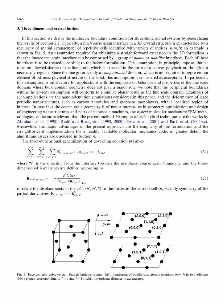
3. Three-dimensional crystal lattices

In this section we derive the multiscale boundary conditions for three-dimensional systems by generalizingthe results of Section 2.2. Typically, a fine/coarse grain interface in a 3D crystal structure is characterized by aregularity of spatial arrangement of repetitive cells identified with triplets of indices (n,m, l); an example isshown in Fig. 5. An assumption required for obtaining a straightforward extension to the 3D formalism isthat the fine/coarse grain interface can be comprised by a group of plane- or slab-like interfaces. Each of theseinterfaces is to be treated according to the below formulation. This assumption, in principle, imposes limita-tions on allowed shapes of the fine grain, which is expected in the form of a convex polyhedron, though notnecessarily regular. Since the fine grain is only a computational domain, which is not required to represent anelement of intrinsic physical structure of the solid, this assumption is considered as acceptable. In particular,this assumption is satisfactory for applications with the emphasis on behavior and properties of the fine scaledomain, where bulk domain geometry does not play a major role; we note that the peripheral boundarieswithin the present assumption will conform to a similar planar setup as the fine scale domain. Examples ofsuch applications are the nanoindentation simulations considered in this paper, and the deformation of largeperiodic nanostructures, such as carbon nanotubes and graphene monolayers, with a localized region ofinterest. In case that the coarse grain geometry is of major interest, as in geometry optimization and designof engineering nanostructures and parts of nanoscale machines, the hybrid molecular mechanics/FEM meth-odologies can be more relevant than the present method. Examples of such hybrid techniques are the works byAbraham et al. (1998), Rudd and Broughton (1998, 2000), Ortiz et al. (2001) and Park et al. (2005b,c).Meanwhile, the major advantages of the present approach are the simplicity of the formulation and thestraightforward implementation for a readily available molecular mechanics code; in greater detail, thealgorithmic issues are discussed in Section 4.

The three-dimensional generalization of governing equation (4) gives

Fig. 5.(001)

Xnþm

n0¼n�m

Xmþl

m0¼m�l

Xlþ1

l0¼l�1

Kn�n0 ;m�m0;l�l0un0 ;m0;l0 ¼ �fn;m;l ð24Þ

where ‘‘l’’ is the direction from the interface towards the peripheral coarse grain boundary, and the three-dimensional K-matrices are defined according to

Kn�n0 ;m�m0;l�l0 ¼ �o

2UðuÞoun;m;l oun0;m0;l0

��u¼0

ð25Þ

to relate the displacements in the cells (n 0,m 0, l 0) to the forces in the current cell (n,m, l). By symmetry of thepartial derivatives, K�n;�m;�l ¼ KT

n;m;l.

(0,1,1)

(1,0,1) (1,2,1)

(2,1,1)

(0,0,0) (0,2,0)

(1,1,0)

(2,0,0) (2,2,0)x, n

y, m

z, l

Face centered cubic crystal: Bravais lattice structure (left); numbering of equilibrium atomic positions (n,m, l) in two adjacentplanes, corresponding to l = 0 and l = 1 (right). Interplanar distance is exaggerated.


Note the distinct character of the third summation in Eq. (24) as compared to the first and second. For theanalysis to follow, we require that the atoms in a given slab of constant l are coupled only to each other and toatoms in the slabs l � 1 and l + 1. For longer-range forces, the size of the unit cell must be increased so thatthis requirement is satisfied. At the same time, the coupling in the directions of indices n and m is not limited toimmediate neighbors, and the parameters m and l of (24) indicate the corresponding maximum order numbersof the interactive cells.

Thus, the task of deriving the 3D multiscale boundary conditions reduces to expressing the atomic displace-ments un,m,1 in terms of un,m,0 and un,m,a,

un;m;1 ¼ Hfun;m;0g þ Nfun;m;ag ð26Þ

where slab l = 0 represents the fine/coarse grain interface, and l = a assigns the coarse grain boundary.Similarly to the 1D case, discussed in Section 2.2, the coarse grain deformation is viewed as due to the exter-

nal forces applied to the atoms (n,m, 0) and (n,m,a)

fn;m;l ¼ dl;0fn;m;0 þ dl;afn;m;a ð27Þ

Next we apply the DFT to Eq. (24) for all three spatial indices, utilizing the external force vector (27) and theconvolution theorem (9) to get the Fourier domain solution

uðp; q; rÞ ¼ Gðp; q; rÞ f0ðp; qÞ þ e�ira faðp; qÞ� �

ð28Þ

Gðp; q; rÞ ¼ �K�1ðp; q; rÞ ð29Þ

We note that within the 3D settings, the DFT can only be utilized for up to three linearly independent spatialdirections; attempts to implement it along additional (linearly dependent) directions may lead to trivial results.Further use of the shift theorem (10) with the inverse (r! l) DFT applied to Eq. (28) yields

~ulðp; qÞ ¼ ~Glðp; qÞf0ðp; qÞ þ ~Gl�aðp; qÞfaðp; qÞ ð30Þ~Glðp; qÞ ¼F�1

r!lfGðp; q; rÞg ð31Þ

where the tilde notations represent the mixed, Fourier/real space, domain quantities; the (r! l) inverseFourier transformation is accomplished in accordance with (8), where p, n and N are replaced with r, l andL = (a + 1)/2, respectively.

Then we write three equations according to (30) by substituting l = 0, l = 1 and l = a, and rearrange themto express the vector ~u1 through ~u0 and ~ua

~u1ðp; qÞ ¼ Hðp; qÞ~u0ðp; qÞ þ Nðp; qÞ~uaðp; qÞ ð32Þ
where
Hðp; qÞ Nðp; qÞ� �

¼ ~G1ðp; qÞ ~G1�aðp; qÞ� � ~G0ðp; qÞ ~G�aðp; qÞ

~Gaðp; qÞ ~G0ðp; qÞ

!�1

ð33Þ

Here, we note the similarity of the 3D Fourier domain equations (32) and (33) with the 1D real space equa-tions (18) and (19).

By applying the inverse DFT for p and q to Eq. (32), and taking into account the convolution theorem (9),we obtain the final form of the 3D multiscale boundary conditions

un;m;1 ¼Xn0 ;m0

Hn�n0 ;m�m0un0 ;m0;0 þXn0 ;m0

Nn�n0 ;m�m0un0 ;m0 ;a ð34Þ

Hn;m ¼F�1p!nF

�1q!mfHðp; qÞg; Nn;m ¼F�1

p!nF�1q!mfNðp; qÞg ð35Þ

The range of the summation indices for computing the inverse DFTs in (35), p 2 [1/2 � N,N � 1/2] and q 2[1/2 �M,M � 1/2], must be such that values 2N and 2M match or exceed lateral dimensions of the coarsegrain along the n and m directions. Then periodic boundary conditions for n and m can be safely assumed.


Thus, the three-dimensional operators of multiscale boundary conditions act as discrete convolution sumsover the interface and coarse grain boundary displacements. These operators are represented by the compactmatrix kernels H and N depending on the lattice geometry and structure of the interatomic potential.

In some applications, including the nanoindentation simulations to be discussed later in this paper, thecoarse scale boundary can be assumed rigidly fixed, so that un,m,a = 0 for all n and m. This assumption sim-plifies Eq. (34) to the form

un;m;1 ¼Xn0;m0

Hn�n0 ;m�m0un0 ;m0 ;0 ð36Þ

In conclusion of this theoretical section, we emphasize that the kernel matrices H and N are dimensionless

quantities, because they relate ‘‘displacements with displacements’’, according to (34) and (36). This indicatesthat, for a given interatomic potential, their values should depend on the geometry of the crystal lattice and thechoice of the elementary cell, rather than on scaling parameters of this potential. This feature is attractive,because it implies the existence of unique kernel matrices for various materials with identical or similar crys-talline structures.

4. Application: nanoindentation of crystalline gold

In this section we verify the three-dimensional formulation on two benchmark nanoindentation problemswith a crystalline gold substrate. For illustrative purposes, we will consider two parallelopipedic configura-tions of the fine grain: (1) with periodic boundary conditions on the side faces, and the multiscale boundaryconditions on the bottom face (Example 1), and (2) with multiscale boundary conditions at five faces (Example2). The top face of the fine grain domain is originally traction free, and it is next subjected to a non-deformableindenter. The first of these geometries represent the simplest case that is equivalent to dealing with a single,formally infinite, plane interface, and the second geometry represents an example of compound interfacesmentioned in the beginning of Section 3.

A substantial part of the substrate is considered as a bulk coarse scale domain, whose atomistic degrees offreedom will be eliminated from the multiscale model. The resultant multiscale solution will be compared withthe benchmark data, obtained by molecular mechanics simulations on the original full domain, i.e., by pre-serving the complete atomistic resolution and all the relevant degrees of freedom at both fine and coarsegrains. The coarse scale boundary displacements in both problems are set to be zero; therefore Eq. (36) willbe utilized.

We introduce the three-dimensional numbering of the atomic locations in the fcc lattice, so that the atomsoccupy the even staggered locations (n,m, l) as illustrated in Fig. 5. Planes with a constant value n, m or l arecoplanar with the crystallographic planes (100), (010) or (001), respectively. We assume the pair-wise Morsepotential for the atomic interactions in gold (e.g., Harrison, 1988)

V ðrÞ ¼ De e2bðq�rÞ � 2ebðq�rÞ De ¼ 0:560 eV; b ¼ 1:637 A

�1; q ¼ 2:922 A

ð37Þ

and will account only for the nearest neighbor interaction in the fcc lattice. In this case, the lattice unit cells arerepresented by single atoms numbered as shown in Fig. 5. For the Cartesian frame depicted in this figure, weobtain the following set of symmetric K-matrices on the basis of expression (25):

K1;1;0 ¼ k

1 1 0

1 1 0

0 0 0

0B@

1CA; K1;�1;0 ¼ k

1 �1 0

�1 1 0

0 0 0

0B@

1CA

K1;0;1 ¼ k

1 0 1

0 0 0

1 0 1

0B@

1CA; K1;0;�1 ¼ k

1 0 �1

0 0 0

�1 0 1

0B@

1CA


K0;1;1 ¼ k

0 0 0

0 1 1

0 1 1

0B@

1CA; K0;1;�1 ¼ k

0 0 0

0 1 �1

0 �1 1

0B@

1CA

K0;0;0 ¼ �8k

1 0 0

0 1 0

0 0 1

0B@

1CA; k ¼ Deb

2 ð38Þ

In greater detail, derivation of these matrices is discussed in Appendix A. Six additional matrices are obtainedfrom (38) by employing K�n,�m,�l = Kn,m,l, while any other subscript triplet (n,m, l) yields a zero matrix. TheFourier transform (7) of these matrices can be derived in a closed form

Kðp; q; rÞ ¼ 4k

ðcos qþ cos rÞ cos p � sin p sin q � sin p sin r

� sin p sin q ðcos p þ cos rÞ cos q � sin q sin r

� sin p sin r � sin q sin r ðcos p þ cos qÞ cos r

0B@

1CA� 8kI ð39Þ

where I is the identity matrix.Further steps in computing the kernel matrix H are accomplished numerically, according to the procedures

(29), (31), (33), (35), and the DFT inversion formula (8).Elements of the matrix H decay quickly with the increase of absolute values of the spatial order parameters

n and m. We illustrate this property by plotting element (1,1) of this matrix in Fig. 6, as a representative func-tion of n at a = 15, the coarse scale parameter, and various m. The overall trends shown are typical for allother elements of H. In accordance with the staggered atomic arrangements in the fcc crystal, matrices Hfor even n + m appear trivial, and they are ignored in Fig. 6 plot. The value of the element (1, 1) is seen todecay by a factor of 100 with the growth of jnj or jmj from 0 to 4. This decay is a valuable property of thekernel matrix. Taking it into account, we can truncate the summation in Eq. (36) at some critical differencesn � n 0 and m � m 0 without a considerable loss of the accuracy. By denoting these critical values as nc and mc,we can update Eq. (36) to give the final form,

un;m;1 ¼Xnþnc

n0¼n�nc

Xmþmc

m0¼m�mc

Hn�n0 ;m�m0un0 ;m0;0 � H � un;m;0 ð40Þ

that has been utilized in our simulations. In most applications with the present fcc model, it is proper to trun-cate this convolution sum at nc, mc = 4–6. This truncation can notably decrease computational cost of themultiscale boundary conditions.

–10 –5 0 5 1010

–4

10–3

10–2

10–1

100

n

m = 0m = 4m = 8

Θn,m

(1,1)

Fig. 6. Typical dependence of the components in the kernel matrix on the values of spatial order parameters.


Another important feature of this kernel matrix is that it is invariant with respect to the value of the inter-action coefficient k in matrices (38), and therefore with respect to parameters of pair-wise potentials. Thus, thepresent kernel matrix H for a given value a is a general characteristic of all monoatomic fcc crystals with thenearest neighbor interaction.

4.1. Algorithmic issues

The conditions (40) provide additional equations for the degrees of freedom at the boundary of the reduceddomain that must be solved simultaneously with the standard molecular mechanics equations for the inner partof the reduced domain. Below, we discuss two possible approaches to such a simultaneous solution. The firstapproach consists in replacing the vectors un,m,1 in the argument of the system�s potential energy function U

with the convolution sums (40),

Uð. . . ; un;m;�1; un;m;0; un;m;1Þ ! UMSð. . . ; un;m;�1; un;m;0;H � un;m;0Þ ð41Þ

for each specific pair of indices n and m. The new function UMS is then sent to a minimization subroutine avail-able in any standard molecular mechanics code. With this approach, the multiscale boundary displacementsun,m,1 will be updated automatically at each iteration step of the energy minimization procedure.

The second approach that we suggest does not involve an update of the potential energy function; instead,it treats specific displacements (40) evaluated at a current iteration step of the minimization process as bound-ary conditions for the next step

Step j : Uð. . . ; un;m;�1; un;m;0; uðj�1Þn;m;1 Þ ! u

ðjÞn;m;0 !

(40)uðjÞn;m;1

Step jþ 1 : Uð. . . ; un;m;�1; un;m;0; uðjÞn;m;1Þ ! u

ðjþ1Þn;m;0 !

(40)uðjþ1Þn;m;1

ð42Þ

The procedure is initialized conventionally by providing an initial guess (trial solution) uð0Þn;m;l for all n, m, and l.

This approach is more attractive for being less involved computationally and easier to program. In some cases,though, it may lead to larger errors, since at the final step, the multiscale boundary conditions will be satisfiedfor the previous iteration only. The choice of a more adequate approach may depend on a specific problemstatement, the nature of a minimization procedure utilized, and the accuracy sought. In the applications dis-cussed below, we adopted the direct method (41) for our final calculations. However, trial usage of the iterativescheme (42) did not compromise performance of the multiscale boundary conditions noticeably.

4.2. Example 1

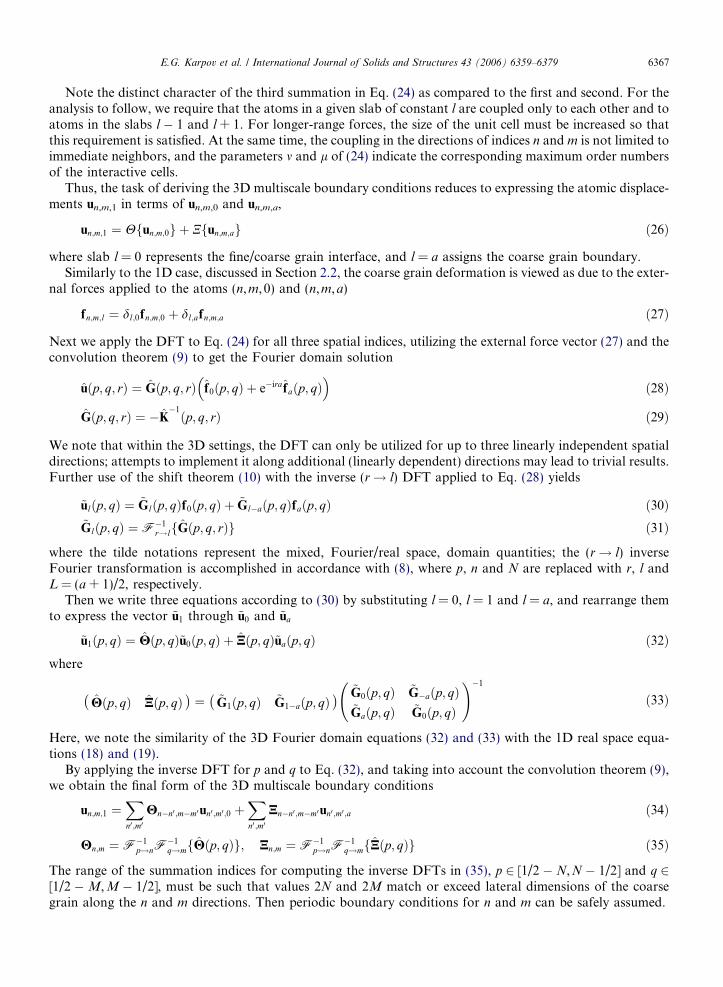
The first problem, depicted in Fig. 7, utilizes the multiscale boundary conditions only at the bottom layer ofthe fine grain domain, while fixed (zero displacement) boundary conditions are applied to the lateral faces. Theatomic displacements along the deformable boundary layer l = 1 in the reduced domain are related with thedisplacements of atoms in the adjacent layer l = 0 through the discrete convolution operator, according to Eq.(40). The original size of the full domain is 17 · 17 · 50 atomic layers, and the fine grain domain (the reduceddomain) comprises 40% of the total volume, i.e., 17 · 17 · 20 layers. This reduction corresponds to the valuea = 31. According to (37), the interlayer distance along the coordinate axes is 2.066 A, and the total height ofthe fine grain is 39.25 A. The curvature radius of the indenter is 10 A. The indentation process is simulated in aseries of iteration steps, where the maximum indentation depth of 6A is achieved at the 60th step. The inter-action between indenter and substrate atoms is modeled with the Lennard Jones potential,

V ðrÞ ¼ 4er12

r12� r6

r6

� �; � ¼ 0:005 eV; r ¼ 2:85 A ð43Þ

where a continuous atomic density of 0.178 atom/A3 is assumed for the indenter (Sokolov and Henderson,2000). We note that alternative models to characterize the tip/substrate interaction can be similarly utilized.

Coarsegrain

Indenter

, ,0un m

, ,1un m

, , =u 0n m a

40%Fine

grain

h

Multiscale BC

Fig. 7. Nanoindentation problem with the multiscale boundary conditions applied at the bottom face of the fine grain; h, height of the fullproblem.


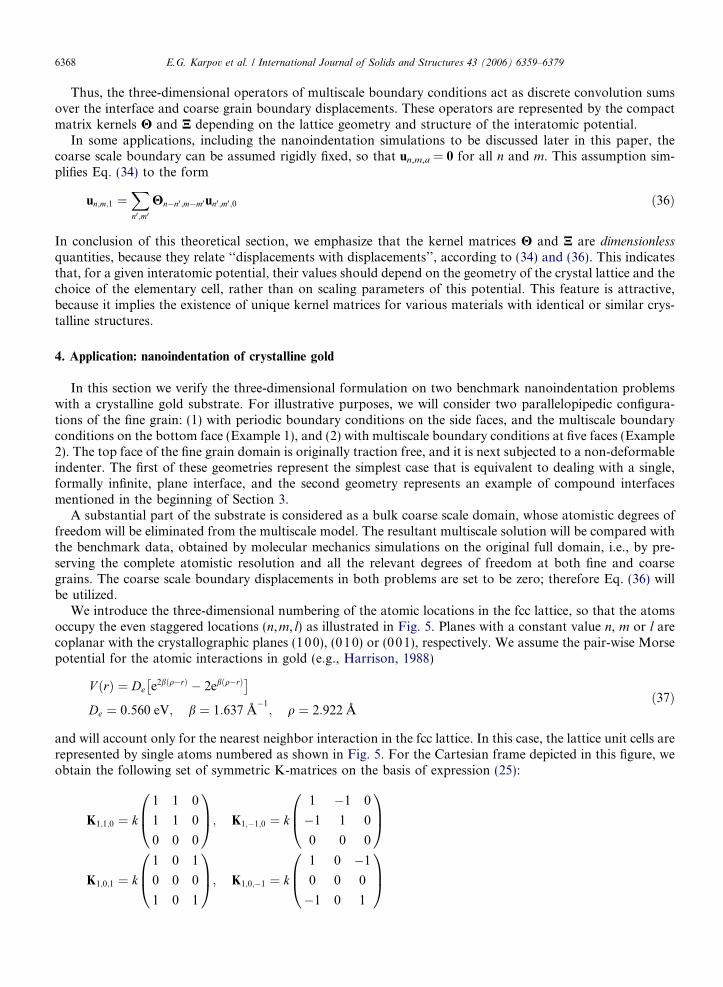
The result of this simulation, the load/indentation depth curve, is plotted in Fig. 8 in comparison with thebenchmark simulation that preserves the complete atomistic resolution for both the fine and coarse grains.The plot shows an excellent agreement between the test (full domain) and multiscale simulations at all threeindentation regimes: elastic load, plasticity (the top part of the indentation curve) and unload. Meanwhile, themultiscale approach reduces the computational effort by a factor of 7.

Fig. 9 shows the structure of dislocations under the indenter tip at the indentation depth 5 A (step 50 inFig. 8). The dislocations were visualized using the following rule. For each specific atom, we computed thenumber of neighbor atoms, Nc, found within a sphere of radius ð1þ

ffiffiffi2pÞq=2, where q is the equilibrium

parameter of the potential (37). This radius is equal to the distance between the current atom and the meanpoint in between the first and the second neighbor shells in the present lattice structure. The coordinationnumber Nc = 12 corresponds to a regular fcc structure, while another value indicates a lattice dislocationor another irregularity. The fcc dislocation cores are most often associated with Nc = 11 and 13; only suchatoms are shown in Fig. 9. It is seen that application of the multiscale boundary conditions allows reproducingof the dislocation picture in very fine details, as compared to the benchmark simulation. At the same time,application of the standard (zero displacement) boundary conditions to the reduced domain violates the pro-cess of dislocations initiation and growth. These results indicate also that the multiscale interface should beestablished on a distance of about 12 {001} planes from the nearest dislocation core to assure good similarityof the results with respect to the corresponding full size problem. We note that indentation of the {00 1}

0 10 20 30 40 50 60

0

0.1

0.2

0.3

0.4

0.5

0.6

0.7

0.8

0.9

1

indentation depth increments

norm

aliz

ed lo

ad

full domainmultiscale, a = 31

loading unloading

Fig. 8. Load vs. indentation depth: comparison of full domain atomistic and multiscale solutions for nanoindentation problem describedin Fig. 7.

Fig. 9. Dislocation structure formed under indenter tip at step 50; comparison for the MSBC approach, and the standard lattice staticssimulations for the benchmark and reduced problems. For the 17 · 17 · 50 case, only the corresponding upper part of the domain isdepicted. The coordination number is 11 and 13 for the light and dark grey atoms, respectively; atoms with other coordination numbersare not shown.

0 10 20 30 40 50 6010

–6

10–5

10–4

10–3

10–2

10–1

mea

n sq

uare

err

or

h

MSBC

Fig. 10. Error estimate for the load/indentation depth dependence in a series of 17 · 17 · h standard full domain simulations, due toboundary effects at the bottom face of the structure. The cross indicates error for the MSBC simulation over the 17 · 17 · 20 domain.


surface results in a compact stacking fault tetrahedra structure under the indenter, imposed by the compact-ness of the structure and the small size of the indenter. Meantime, indentation into a surface where {111} slipplanes are parallel to the indentation direction may result in a long-range motion of dislocations, and thereforein a larger fine scale domain to be utilized.

The size of the benchmark problem was chosen on the basis of the following. Initially, a series of molecularmechanics simulations were accomplished over the domains 17 · 17 · h of various heights h (see Fig. 7), com-prised of 10–60 layers with 10 layer increments. The standard zero displacement boundary conditions appliedat the bottom and side faces of the structure. All other provisos, including the indenter size at the total inden-tation depth were kept invariant, identical to the above problem statement. The mean square error was eval-uated for all load/indentation depth dependencies at h < 60 with respect to the curve corresponding to h = 60.The error stabilizes at h P 40 (see Fig. 10) and the indentation curves were found identical at h = 50 and 60 inall indentation regimes. Thus, the domain comprised of 50 atomic layers in height was considered as the min-imal structure, required for the standard lattice statics simulations within the current problem settings.

4.3. Example 2

The second problem employs the multiscale boundary conditions separately at five planar faces of the par-allelepiped fine grain, excluding the top traction free boundary, which is exposed to the indenter (see Fig. 11).

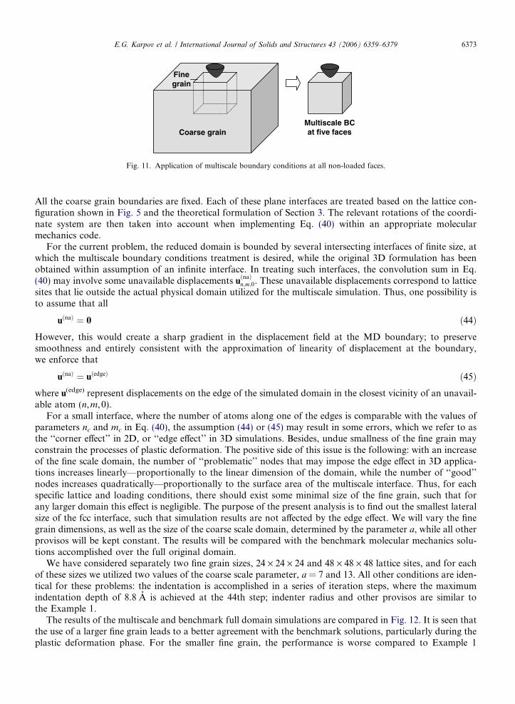
Finegrain

Coarse grainMultiscale BCat five faces

Fig. 11. Application of multiscale boundary conditions at all non-loaded faces.


All the coarse grain boundaries are fixed. Each of these plane interfaces are treated based on the lattice con-figuration shown in Fig. 5 and the theoretical formulation of Section 3. The relevant rotations of the coordi-nate system are then taken into account when implementing Eq. (40) within an appropriate molecularmechanics code.

For the current problem, the reduced domain is bounded by several intersecting interfaces of finite size, atwhich the multiscale boundary conditions treatment is desired, while the original 3D formulation has beenobtained within assumption of an infinite interface. In treating such interfaces, the convolution sum in Eq.(40) may involve some unavailable displacements u

ðnaÞn;m;0. These unavailable displacements correspond to lattice

sites that lie outside the actual physical domain utilized for the multiscale simulation. Thus, one possibility isto assume that all

uðnaÞ ¼ 0 ð44Þ
However, this would create a sharp gradient in the displacement field at the MD boundary; to preservesmoothness and entirely consistent with the approximation of linearity of displacement at the boundary,we enforce that
uðnaÞ ¼ uðedgeÞ ð45Þ
where u(edge) represent displacements on the edge of the simulated domain in the closest vicinity of an unavail-able atom (n,m, 0).
For a small interface, where the number of atoms along one of the edges is comparable with the values ofparameters nc and mc in Eq. (40), the assumption (44) or (45) may result in some errors, which we refer to asthe ‘‘corner effect’’ in 2D, or ‘‘edge effect’’ in 3D simulations. Besides, undue smallness of the fine grain mayconstrain the processes of plastic deformation. The positive side of this issue is the following: with an increaseof the fine scale domain, the number of ‘‘problematic’’ nodes that may impose the edge effect in 3D applica-tions increases linearly—proportionally to the linear dimension of the domain, while the number of ‘‘good’’nodes increases quadratically—proportionally to the surface area of the multiscale interface. Thus, for eachspecific lattice and loading conditions, there should exist some minimal size of the fine grain, such that forany larger domain this effect is negligible. The purpose of the present analysis is to find out the smallest lateralsize of the fcc interface, such that simulation results are not affected by the edge effect. We will vary the finegrain dimensions, as well as the size of the coarse scale domain, determined by the parameter a, while all otherprovisos will be kept constant. The results will be compared with the benchmark molecular mechanics solu-tions accomplished over the full original domain.

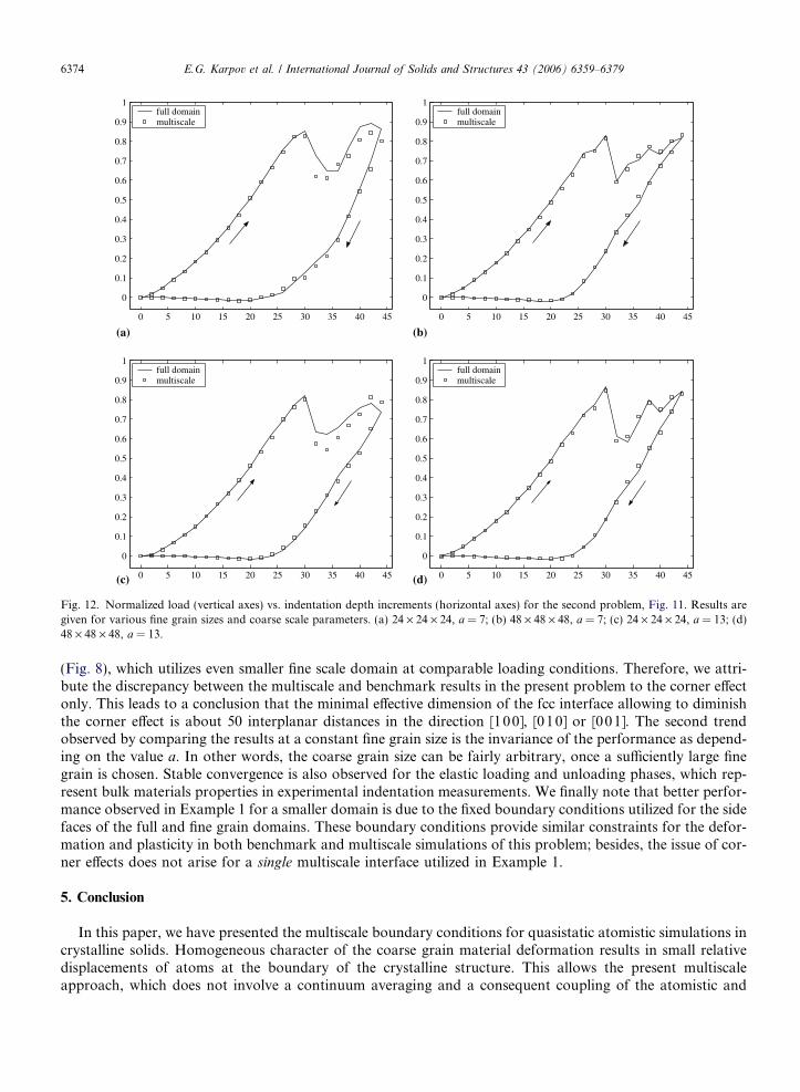
We have considered separately two fine grain sizes, 24 · 24 · 24 and 48 · 48 · 48 lattice sites, and for eachof these sizes we utilized two values of the coarse scale parameter, a = 7 and 13. All other conditions are iden-tical for these problems: the indentation is accomplished in a series of iteration steps, where the maximumindentation depth of 8.8 A is achieved at the 44th step; indenter radius and other provisos are similar tothe Example 1.

The results of the multiscale and benchmark full domain simulations are compared in Fig. 12. It is seen thatthe use of a larger fine grain leads to a better agreement with the benchmark solutions, particularly during theplastic deformation phase. For the smaller fine grain, the performance is worse compared to Example 1

0 5 10 15 20 25 30 35 40 45

0

0.1

0.2

0.3

0.4

0.5

0.6

0.7

0.8

0.9

1full domainmultiscale

(a) (b)

(c) (d)

0 5 10 15 20 25 30 35 40 45

0

0.1

0.2

0.3

0.4

0.5

0.6

0.7

0.8

0.9


0 5 10 15 20 25 30 35 40 45

0

0.1

0.2

0.3

0.4

0.5

0.6

0.7

0.8

0.9


0 5 10 15 20 25 30 35 40 45

0

0.1

0.2

0.3

0.4

0.5

0.6

0.7

0.8

0.9


Fig. 12. Normalized load (vertical axes) vs. indentation depth increments (horizontal axes) for the second problem, Fig. 11. Results aregiven for various fine grain sizes and coarse scale parameters. (a) 24 · 24 · 24, a = 7; (b) 48 · 48 · 48, a = 7; (c) 24 · 24 · 24, a = 13; (d)48 · 48 · 48, a = 13.


(Fig. 8), which utilizes even smaller fine scale domain at comparable loading conditions. Therefore, we attri-bute the discrepancy between the multiscale and benchmark results in the present problem to the corner effectonly. This leads to a conclusion that the minimal effective dimension of the fcc interface allowing to diminishthe corner effect is about 50 interplanar distances in the direction [100], [010] or [001]. The second trendobserved by comparing the results at a constant fine grain size is the invariance of the performance as depend-ing on the value a. In other words, the coarse grain size can be fairly arbitrary, once a sufficiently large finegrain is chosen. Stable convergence is also observed for the elastic loading and unloading phases, which rep-resent bulk materials properties in experimental indentation measurements. We finally note that better perfor-mance observed in Example 1 for a smaller domain is due to the fixed boundary conditions utilized for the sidefaces of the full and fine grain domains. These boundary conditions provide similar constraints for the defor-mation and plasticity in both benchmark and multiscale simulations of this problem; besides, the issue of cor-ner effects does not arise for a single multiscale interface utilized in Example 1.

5. Conclusion

In this paper, we have presented the multiscale boundary conditions for quasistatic atomistic simulations incrystalline solids. Homogeneous character of the coarse grain material deformation results in small relativedisplacements of atoms at the boundary of the crystalline structure. This allows the present multiscaleapproach, which does not involve a continuum averaging and a consequent coupling of the atomistic and


continuum models. As a result, the method does not involve an artificial handshake region. It utilizes spatialregularity of crystalline solids, and enables one to calculate the quasistatic response of the coarse grain, theperipheral elastic domain, on the intrinsic atomic level. The lattice translation symmetry along the fine/coarsegrain interface is employed by means of the discrete Fourier transform to yield a compact formulation in termsof a discrete convolution operator. This operator represents the response behavior of the coarse grain, andprovides boundary conditions for the atomistic simulation over a localized domain of interest. As a result,the computer simulations can be run for the localized atomistic domain only, while all the coarse grain degreesof freedom are eliminated. This gives a possibility for drastic savings in computational time—up to severalorders of the magnitude. The method is most adequate in applications to problems with simple coarse graingeometries, where the peripheral boundaries follow a planar setup, similar to one chosen for the multiscaleinterface, i.e., for the boundary of the local region of interest. In problems with complex coarse scale geom-etries and force distributions, the available hybrid multiscale techniques can be more versatile. The majoradvantages of the present approach in comparison with the hybrid techniques are the simplicity of the finalworking formulation, Eq. (18) or (34), and the straightforward implementation for a readily available molec-ular mechanics energy minimization code.

This method has been verified in a series of nanoindentation simulations. The multiscale boundary condi-tions according to (40) have been shown to perform well for a wide range of indentation depths and methodparameters, where a good agreement with the benchmark full domain solution was observed. All threeregimes, elastic load, plastic deformation of the substrate around the indenter tip, and unload were reproducedadequately. Plastic behavior is implied by bond breaking processes within the fine grain domain, and it is rep-resented by the discontinuous character at a later phase of the loading process. The non-linear/plastic behav-ior is allowed inside the simulated domain, because the formulation assumes linearity only in the vicinity of theinterface between the atomistic and peripheral elastic domains. Regarding the performance of the method,there are two general guidelines that can enable the practitioner to determine an adequate, yet computation-ally effective fine/coarse grain partitioning: (1) performance of the multiscale boundary conditions improveswith the increase of a fine grain, and (2) performance is typically invariant with respect to the size of a coarsegrain. In other words, once a sufficiently large fine grain is chosen, linear dimensions of the coarse grain can befairly arbitrary. Applicability conditions, which guarantee good performance of this method, can be summa-rized as the following: (1) the coarse grain and the fine/coarse grain interface are dislocation-free, and theirdeformation is linear elastic (in the hypothetical fully atomistic model); (2) linear dimension of the fine grainin the corresponding lattice direction is larger than the length occupied 50 unit cells. The second of these con-ditions has to be satisfied in order to eliminate corner effects in applications to two- and three-dimensionalstructures.

Properties of the kernel matrices of the interface operator have been investigated on an fcc gold lattice witha pair-wise potential. Components of these matrices appear to decay quickly with the growth of spatial orderparameters; this allows truncating the corresponding convolution summations and leads to the numerical effi-ciency of this method. Another interesting property of the kernel matrices is their invariance with respect tothe choice of the interatomic potential, so that it serves as a fundamental characteristic of the fcc geometrywith the nearest neighbor interaction. Furthermore, a general systematic analysis of the asymptotic and invari-ant properties of the multiscale operators is an objective for future.

A fully self-consistent dynamic formulation of this method, involving also recognition of dislocation pat-terns and their passage to the coarse grain, is also a future challenge. Similar to other multiscale approaches,the current method requires a priori knowledge of the non-linear plastic zone; exclusions are the QC method,e.g., Ortiz et al. (2001), and the method by Shilkrot et al. (2004). However, localized inhomogeneities, such asthe lattice dislocations, can be arranged to pass the multiscale interface and absorbed by the coarse scaleregion within a straightforward extension, which will be discussed in a future publication. The basic idea willconsist in early identification of a dislocation in a release zone within the fine grain, and redefining the fine/coarse interface after the dislocation is transferred through the interface. The authors are also working onapplications of the present methodology to periodic nanostructures, such as carbon nanotubes, nanowiresand graphene monolayers, e.g. Medyanik et al. (2005). A broader task for the future consists in creation ofa database of the kernel matrices corresponding to major Bravais lattices governed by popular interatomic


potentials, including the many-body potentials. This database, once available, could serve as a valuableresource for extensive usage by the computational mechanics community.

Acknowledgement

The authors would like to express their sincere gratitude to the support from the US National ScienceFoundation and Office of Naval Research.

Appendix A

A.1. Discrete Fourier transform

The inversion formula (8) for a finite sequence can be derived on the basis of the following. First note thatany finite sequence {gn} at n 2 [nmin,nmax], can be considered formally as an infinite sequence at n 2 [�1,1]with all zero elements in the range n < nmin and n > nmax. Most generally, the inverse DFT of such a sequencecan be evaluated as an integral of the 2p-periodic function (7),

gn ¼1

2p

Z p

�pgðpÞeipn dp ðA:1Þ

Indeed, employ the DFT in the form (7) for the above integral and rearrange it to get

1

2p

Z p

�p

Xn0

gn0e�ipn0eipn dp ¼ 1

2p

Xn0

gn0

Z p

�pe�ipðn0�nÞ dp ¼

Xn0

gn0dn;n0 ¼ gn ðA:2Þ

Here, d is the Kronecker delta; n and n 0 are integers.The integral (A.1) can be approximated by applying the midpoint integration rule,
Z b
af ðxÞdx � h f

x0 þ x1

2

� � þ f

xJ�1 þ xJ

2

� �h i; h ¼ b� a

J; xk ¼ aþ hk ðA:3Þ

If the wave number p is discretized as

p ¼ pvp

N; vp ¼ �

1

2;� 3

2; . . . ;�N 1

2ðA:4Þ

then application of the midpoint rule to (A.1) yields

gn �1

2N

XN�1=2

vp¼1=2�N

gpvp

N

� �eipvpn=N ðA:5Þ

The value 2N must correspond to the range of non-trivial elements in the original real space sequence {gn}, i.e.,2N = nmax � nmin + 1.

The nature of Fourier integrals is such that discretization procedures of the type (A.4) and (A.5) yield theexact real space sequences. Indeed,

1

2N

XN�1=2

vp¼1=2�N

gpvp

N

� �eipvpn=N ¼ 1

2N

XN�1=2

vp¼1=2�N

Xn0

gn0e�ipvpn0=N

!eipvpn=N

¼ 1

2N

Xn0

gn0

XN�1=2

vp¼1=2�N

e�ipvpn0=N eipvpn=N ¼X

n0gn0dn;n0 ¼ gn ðA:6Þ

Thus, we can employ an equality sign in (A.5) and obtain the inversion formula (8).


The convolution theorem (9) can be proved as the following:

Fig. Alatticefound

FX

n0fn�n0gn0

( )¼X

n

Xn0

fn�n0gn0e�ipn ¼

Xn

Xn0

fn�n0gn0e�ipðn�n0Þe�ipn0

¼X

n0

Xn

fn�n0e�ipðn�n0Þgn0e

�ipn0 ¼X

n0f ðpÞgn0e

�ipn0 ¼ f ðpÞgðpÞ ðA:7Þ

Note that the range of summations in the above relationships is, in principle, from �1 to 1.The shift theorem (10) is proved by utilizing a similar procedure

Ffgnþhg ¼X

n

gnþhe�ipn ¼X

n

gnþhe�ipðnþhÞeiph ¼ gðpÞeiph ðA:8Þ

where value h is integer.

A.2. Derivation of K-matrices

There exist two approaches to practical implementation of the symbolic expression (25). The first of these isa numerical approach consisting in the following. Consider a numerical model of the regular fcc structure,where all atoms are rigidly fixed at the equilibrium positions; for a lattice governed by (37), these positionsare determined by the radius vectors

reqn;m;l ¼

qffiffiffi2p

n

m

l

0B@

1CA; nþ mþ l� even ðA:9Þ

where n, m and l is the atomic numbering shown in Fig. 5. The frame origin is associated with the atom (0, 0,0)(see Fig. A.1). Within the nearest neighbor interaction assumption, atoms associated with the vectors (A.9)also serve as the lattice unit cells. The numerical model must include the cell at origin and all the adjacent cellsinteracting directly with it. Thus, we construct a numerical model for the atom (0,0,0) and its 12 closest neigh-bors of the type shown in Fig. A.1.

On the next stage we perturb the equilibrium position of the origin atom (0,0,0) along the x-axis by a smallvalue dx0,0,0� q, while all other atoms are kept fixed at the initial positions (A.9). Then we measure (i.e., eval-uate numerically) three components of the force exerted on the atom at origin due such a perturbation: f x, f y

and f z. The ratios of these forces with respect to the value of displacement dx0,0,0 comprise the first column ofthe matrix K0,0,0. This procedure is repeated by perturbing the y- and z-axis positions of the origin atom atdy0,0,0� q and dz0,0,0� q, accordingly, in order to obtain two remaining columns of the matrix K0,0,0. Theposition perturbation procedure is repeated also for the 12 neighboring atoms, while the force components

(1,1,0)x

y

(0,1,1)

(0,0,0)

(1,0,1)

ρ

ρρ

z

.1. Three nearest neighbors for the current atom (0,0,0) in the fcc structure. There are in total 12 such neighbors for each specificatom; for the atom at origin, these are (±1,±1,0), (±1,0,±1), (0,±1,±1), (±1,1,0), (±1,0,1) and (0,±1,1). The neighbors areat the equilibrium distance q, which is considered as a parameter of the interatomic potential (37).


f x, f y and f z are still measured at the origin atom. For each specific neighbor atom (n,m, l), one additionalmatrix K�n,�m,�l is assembled. In general, the above procedure can be expressed by the following:

K�n;�m;�l �

f x

dxn;m;l

f x

dyn;m;l

f x

dzn;m;l

f y

dxn;m;l

f y

dyn;m;l

f y

dzn;m;l

f z

dxn;m;l

f z

dyn;m;l

f z

dzn;m;l

0BBBBBBB@

1CCCCCCCA; nþ mþ l� even ðA:10Þ

Matrices for odd n + m + l are regarded to be trivial.For relatively simple potentials of interaction, one may also exercise the following analytical approach to

the derivation of K-matrices. This approach is exact, though it may appear intractable for complex long-ran-ged potentials. In below we discuss this technique in application to the present fcc model. Consider the latticepotential energy associated with the interaction of the current atom (0, 0,0) with its neighbors within the rangeof the interatomic potential. This energy is given 12 pair-wise terms in the form

U ¼ V ðjr1;1;0 � r0;0;0jÞ þ V ðjr1;0;1 � r0;0;0jÞ þ . . .10 analogous terms

ðA:11Þ

where V is the Morse potential (25). The variable vectors rn,m,l describe current positions of atoms (n,m, l) in adeformed lattice. These vectors can be replaced by the sums,

rn;m;l ¼ reqn;m;l þ un;m;l ðA:12Þ

where reqn;m;l is the constant vector (A.9), and un;m;l ¼ ðux

n;m;l; uyn;m;l; u

zn;m;lÞ is the variable vector of displacements of

the atom (n,m, l). Then the arguments of function V in Eq. (A.11) can be rewritten as

jrn;m;l � r0;0;0j ¼ jreqn;m;l þ un;m;l � r

eq0;0;0 � u0;0;0j

¼ nqffiffiffi2p þ ux

n;m;l � ux0;0;0

� �2

þ mqffiffiffi2p þ uy

n;m;l � uy0;0;0

� �2

þ lqffiffiffi2p þ uz

n;m;l � uz0;0;0

� �2" #1

2

ðA:13Þ

Substitution of these arguments into (A.11), provides the potential energy in terms of the atomic displace-ments, i.e., U(u) symbolically. Finally, the K-matrices are derived by evaluating the second derivatives (25)in closed form,

K�n;�m;�l ¼ Kn;m;l ¼ �

o2UðuÞoux

0;0;0 ouxn;m;l

o2UðuÞoux

0;0;0 ouyn;m;l

o2UðuÞoux

0;0;0 ouzn;m;l

o2UðuÞouy

0;0;0 ouxn;m;l

o2UðuÞouy

0;0;0 ouyn;m;l

o2UðuÞouy

0;0;0 ouzn;m;l

o2UðuÞouz

0;0;0 ouxn;m;l

o2UðuÞouz

0;0;0 ouyn;m;l

o2UðuÞouz

0;0;0 ouzn;m;l

0BBBBBBBBB@

1CCCCCCCCCA

u¼0

ðA:14Þ

followed by replacing the displacement components, uxn;m;l, uy

n;m;l and uzn;m;l, with zeros at all n, m and l. The later

procedure is symbolized by the subscript notation u = 0. Derivation of the closed form derivatives for (A.14) isconvenient by utilizing symbolic tools of Maple or Mathematica software packages.

References

Abraham, F.F., Broughton, J.Q., Bernstein, N., Kaxiras, E., 1998. Spanning the continuum to quantum length scales in a dynamicsimulation of brittle fracture. Europhysics Letters 44 (6), 783–787.

Broughton, J.Q., Abraham, F.F., Bernstein, N., Kaxiras, E., 1999. Concurrent coupling of length scales: methodology and application.Physical Review B 60 (4), 2391–2403.

Curtin, W.A., Miller, R.E., 2003. Atomistic/continuum coupling in computational materials science. Modelling and Simulation inMaterials Science and Engineering 11, R33–R68.


Deymier, P.A., Vasseur, J.O., 2002. Concurrent multiscale model of an atomic crystal coupled with elastic continua. Physical Review B 66(13), 134106.

Harrison, D.E., 1988. Application of molecular dynamics simulations to the study of ion-bombarded metal surfaces. Critical Reviews inSolid State and Materials Science 14 (Sup.1), S1–S78.

Karpov, E.G., Stephen, N.G., Dorofeev, D.L., 2002. On static analysis of finite repetitive structures by discrete Fourier transform.International Journal of Solids and Structures 39 (16), 4291–4310.

Karpov, E.G., Stephen, N.G., Liu, W.K., 2003. Initial tension in randomly disordered periodic lattices. International Journal of Solidsand Structures 40 (20), 5371–5388.

Karpov, E.G., Wagner, G.J., Liu, W.K., 2005. A Green�s function approach to deriving wave-transmitting boundary conditions inmolecular dynamics simulations. International Journal for Numerical Methods in Engineering 62 (9), 1250–1262.

Liu, W.K., Karpov, E.G., Zhang, S., Park, H.S., 2004. An introduction to computational nano mechanics and materials. ComputerMethods in Applied Mechanics and Engineering 193 (17–20), 1529–1578.

Medyanik, S.A., Karpov, E.G., Liu, W.K., 2005. Domain reduction method for atomistic simulations. Journal of Computational Physics,submitted for publication.

Ortiz, M., Cuitino, A.M., Knap, J., Koslowski, M., 2001. Mixed atomistic continuum models of material behavior: the art of transcendingatomistics and informing continua. MRS Bulletin 26 (3), 216–221.

Park, H.S., Karpov, E.G., Liu, W.K., 2005a. Non-reflecting boundary conditions for atomistic, continuum and coupled atomistic/continuum simulations. International Journal for Numerical Methods in Engineering 64, 237–259.

Park, H.S., Karpov, E.G., Liu, W.K., Klein, P.A., 2005b. The bridging scale for two-dimensional atomistic/continuum coupling.Philosophical Magazine 85 (1), 79–113.

Park, H.S., Karpov, E.G., Klein, P.A., Liu, W.K., 2005c. Three-dimensional bridging scale analysis of dynamic fracture. Journal ofComputational Physics 207, 588–609.

Rudd, R.E., Broughton, J.Q., 1998. Coarse-grained molecular dynamics and the atomic limit of finite elements. Physical Review B 58 (10),R5893–R5896.

Rudd, R.E., Broughton, J.Q., 2000. Concurrent coupling of length scales in solid state systems. Physica Status Solidi B 217 (1), 251–291.Ryvkin, M., Fuchs, M.B., Nuller, B., 1999. Optimal design of infinite repetitive structures. Structural Optimization 18 (2–3), 202–209.Shenoy, V.B., Miller, R., Tadmor, E.B., Phillips, R., Ortiz, M., 1998. Quasicontinuum models of interfacial structure and deformation.

Physical Review Letters 80 (4), 742–745.Shilkrot, L.E., Miller, R.E., Curtin, W.A., 2004. Multiscale plasticity modeling: coupled atomistics and discrete dislocation mechanics.

Journal of the Mechanics and Physics of Solids 52 (4), 755–787.Sokolov, I.Y., Henderson, G.S., 2000. The height dependence of image contrast when imaging by non-contact afm. Surface Science 464

(2–3), L745–L751.Tadmor, E.B., Phillips, R., Ortiz, M., 1996. Mixed atomistic and continuum models of deformation in solids. Langmuir 12 (19), 4529–

4534.Wagner, G.J., Liu, W.K., 2003. Coupling of atomistic and continuum simulations using a bridging scale decomposition. Journal of

Computational Physics 190, 249–274.Wagner, G.J., Karpov, E.G., Liu, W.K., 2004. Molecular dynamics boundary conditions for regular crystal lattices. Computer Methods in

Applied Mechanics and Engineering 193 (17–20), 1579–1601.

Multiscale boundary conditions in crystalline solids...

Documents

Transcript of Multiscale boundary conditions in crystalline solids...