Multiresolution Matrix Compression

Nedelina Teneva Pramod K Mudrakarta Risi KondorDepartment of Computer Science

The University of Chicagonteneva@uchicago.edu

Department of Computer ScienceThe University of Chicago

pramodkm@uchicago.edu

Department of Computer ScienceDepartment of Statistics

The University of Chicagorisi@uchicago.edu

Abstract

Multiresolution Matrix Factorization (MMF) isa recently introduced method for finding multi-scale structure and defining wavelets on graphsand matrices. MMF can also be used for ma-trix compression (sketching). However, the orig-inal MMF algorithm of (Kondor et al., 2014)scales with n3 or worse (where n is the num-ber of rows/columns in the matrix to be factor-ized) making it infeasible for large scale prob-lems. In this paper we describe pMMF, a fast par-allel MMF algorithm, which can scale to n in therange of millions. Our experimental results showthat when used for matrix compression, pMMFoften achieves much lower error than competingalgorithms (especially on network data), yet forsparse matrices its running time scales close tolinearly with n.

1 INTRODUCTION

The massive size of modern datasets often requires matri-ces arising in learning problems to be reduced in size. Dis-tance matrices or Gram (kernel) matrices, in particular, areoften a computational bottleneck, because they are largeand dense. Assuming that the number of data points isn, the space complexity of these matrices is n2, while thetime complexity of the linear algebra operations involvedin many learning algorithms, such as eigendecomposition,matrix inversion, or solving least squares problems, usuallyscales with n3. Without efficient matrix compression (or, asthey are sometimes called, sketching) methods, many pop-ular machine learning algorithms are simply inapplicable totoday’s datasets, where n is often on the order of millions.

The most classical method for compressing a symmetric

Appearing in Proceedings of the 19th International Conferenceon Artificial Intelligence and Statistics (AISTATS) 2016, Cadiz,Spain. JMLR: W&CP volume 51. Copyright 2016 by the authors.

matrix A∈Rn×n is Principle Component Analysis (PCA),which projects A onto the subspace spanned by its k lead-ing eigenvectors (Eckart and Young, 1936). PCA is optimalin the sense that the projection minimizes the reconstruc-tion error of A measured in terms of any of the three mostcommon matrix norms: Frobenius, operator, or nuclear.The main drawback of PCA is its computational complex-ity — calculating the k leading eigenvectors of A, unless Ais very sparse, costs O(kn2), which is often prohibitive.

To address this issue, in recent years randomized sketch-ing methods have become very popular. These algorithmscome in three main flavors (see (Woodruff, 2014) for a re-cent review):

1. Dense projection methods project A to a random sub-space spanned by a small number of dense random vec-tors and use Johnson–Lindenstrauss type arguments toshow that this preserves most of the structure (Halkoet al., 2011);

2. Row/column sampling methods (when A is positivesemi-definite, usually called Nystrom methods) con-struct an approximation to A from a small subset of itsrows/columns sampled from a carefully chosen proba-bility distribution (Smola and Schokopf, 2000; Fowlkeset al., 2004; Drineas and Mahoney, 2005; Deshpandeet al., 2006; Kumar et al., 2009; Zhang and Kwok,2010; Wang and Zhang, 2013; Gittens and Mahoney,2013);

3. Structured sparsity based methods combine the ad-vantages of (i) and (ii) by sampling a small number ofrows/columns, but after applying a dense but efficientlycomputable transformation, such as an FFT (Ailon andChazelle, 2010; Martinsson, 2008).

What all of the above randomized algorithms have in com-mon is the underlying assumption that A has low rank, orat least that it can be well modeled by a low rank surro-gate. Recently, however, a number of authors have pro-posed multiresolution structure as an alternative to the lowrank paradigm, especially in the context of graph/networkdata (Ravasz and Barabasi, 2003; Coifman and Maggioni,2006; Savas et al., 2011). Multiresolution Matrix Fac-

Multiresolution Matrix Compression

torization (MMF) applies these ideas to matrices directly(Kondor et al., 2014), and has been proposed as an alter-native to 1–3 for matrix sketching. However, the actualalgorithm described in (Kondor et al., 2014) for comput-ing MMF factorizations has time complexity O(n3) (or aneven higher power n for higher order rotations), ruling outits use on large datasets.

The present paper describes the first practical MMF–basedapproach to matrix sketching, bypassing the limitations of(Kondor et al., 2014) by introducing a new, fast parallelMMF algorithm called pMMF. Our experiments show that

1. When A is sparse, pMMF can easily scale to n in therange of millions even on modest hardware.

2. For many matrices of interest, the wall clock runningtime of pMMF is close to linear in n.

3. The compression error of the resulting MMF-basedsketching scheme is often much lower than that of theother sketching methods.

The code for pMMF has been made publicly available inthe form of a C++ software library distributed under theGNU Public License v.3.0. (Kondor et al., 2015).

2 MATRIX COMPRESSION WITH MMF

In the following, [n] will denote the set {1, 2, . . . , n}.Given a matrix A ∈Rn×n and two (ordered) sets S1, S2 ⊆[n], AS1,S2

will denote the |S1|×|S2| dimensional subma-trix of A cut out by the rows indexed by S1 and the columnsindexed by S2. S will denote the complement of S, in [n],i.e., [n]\S. B1∪· B2∪· . . .∪· Bm = [n] denotes that the or-dered sets B1, . . . , Bm form a partition of [n]. A:,i or [A]:,idenotes the i’th column of A.

2.1 The MMF Sketching Model

The Multiresolution Matrix Factorization (MMF) of a sym-metric matrix A∈Rn×n is a multi-level factorization of theform

A ≈ Q⊤1 . . . Q⊤

L−1Q⊤LH QLQL−1 . . . Q1, (1)

where Q1, . . . , QL is a sequence of carefully chosen or-thogonal matrices (rotations) obeying the following con-straints:

MMF1. Each Qℓ is chosen from some subclass Q ofhighly sparse orthogonal matrices. In the simplestcase, Q is the class of Givens rotations, i.e., or-thogonal matrices that only differ from the iden-tity matrix in four matrix elements

[Qℓ]i,i = cos θ, [Qℓ]i,j = − sin θ,

[Qℓ]j,i = sin θ, [Qℓ]j,j = cos θ,

for some pair of indices (i, j) and rotation angleθ. Slightly more generally, Q can be the class of

so-called k–point rotations, which rotate not justtwo, but k coordinates, (i1, . . . , ik). Note that theGivens rotation case corresponds to k=2.

MMF2. The effective size of the rotations decreases ac-cording to a set schedule n = δ0 ≥ δ1 ≥ . . . ≥δL, i.e., there is a nested sequence of sets [n] =S0 ⊇ S1 ⊇ . . . ⊇ SL with |Sℓ| = δℓ such that[Qℓ]Sℓ−1,Sℓ−1

is the n−δℓ−1 dimensional identity.Sℓ is called the active set at level ℓ. In the simplestcase, exactly one row/column is removed from theactive set after each rotation.

MMF3. H is SL–core-diagonal, which means that allits entries are zero, except for (a) the submatrix[H]SL,SL

called the core, and (b) the rest of thediagonal.

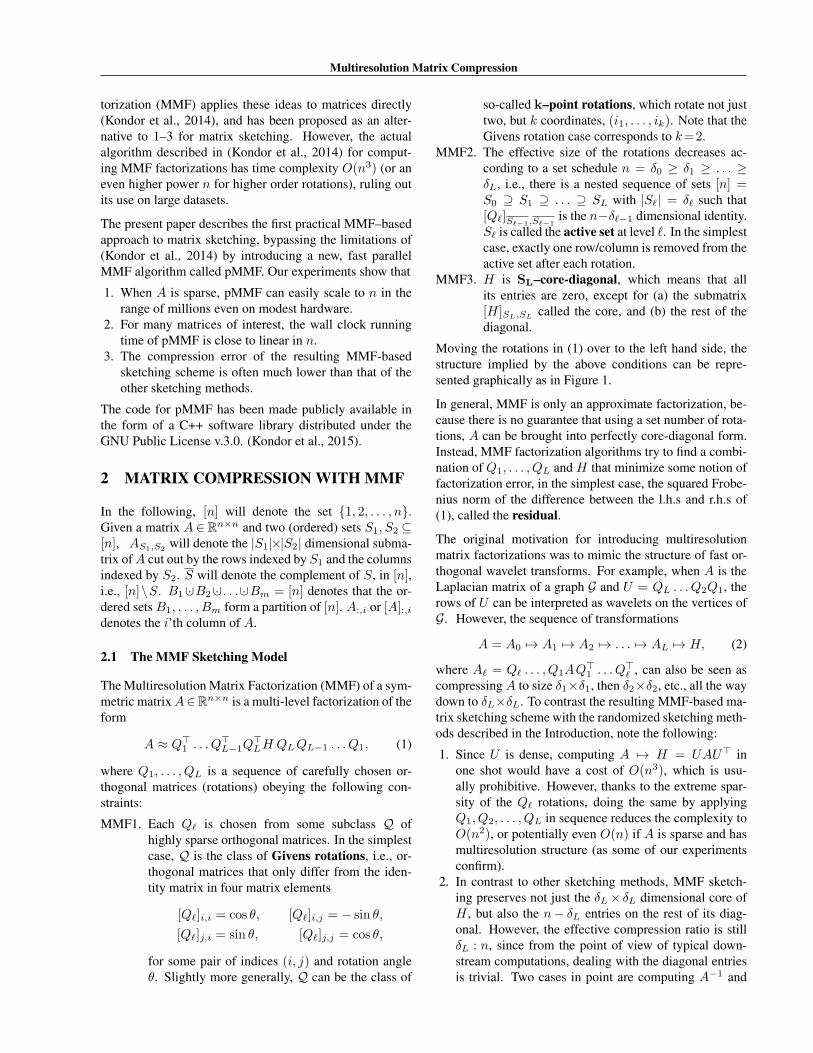
Moving the rotations in (1) over to the left hand side, thestructure implied by the above conditions can be repre-sented graphically as in Figure 1.

In general, MMF is only an approximate factorization, be-cause there is no guarantee that using a set number of rota-tions, A can be brought into perfectly core-diagonal form.Instead, MMF factorization algorithms try to find a combi-nation of Q1, . . . , QL and H that minimize some notion offactorization error, in the simplest case, the squared Frobe-nius norm of the difference between the l.h.s and r.h.s of(1), called the residual.

The original motivation for introducing multiresolutionmatrix factorizations was to mimic the structure of fast or-thogonal wavelet transforms. For example, when A is theLaplacian matrix of a graph G and U = QL . . . Q2Q1, therows of U can be interpreted as wavelets on the vertices ofG. However, the sequence of transformations

A = A0 7→ A1 7→ A2 7→ . . . 7→ AL 7→ H, (2)

where Aℓ = Qℓ . . . , Q1AQ⊤1 . . . Q⊤

ℓ , can also be seen ascompressing A to size δ1×δ1, then δ2×δ2, etc., all the waydown to δL×δL. To contrast the resulting MMF-based ma-trix sketching scheme with the randomized sketching meth-ods described in the Introduction, note the following:

1. Since U is dense, computing A 7→ H = UAU⊤ inone shot would have a cost of O(n3), which is usu-ally prohibitive. However, thanks to the extreme spar-sity of the Qℓ rotations, doing the same by applyingQ1, Q2, . . . , QL in sequence reduces the complexity toO(n2), or potentially even O(n) if A is sparse and hasmultiresolution structure (as some of our experimentsconfirm).

2. In contrast to other sketching methods, MMF sketch-ing preserves not just the δL× δL dimensional core ofH , but also the n− δL entries on the rest of its diag-onal. However, the effective compression ratio is stillδL : n, since from the point of view of typical down-stream computations, dealing with the diagonal entriesis trivial. Two cases in point are computing A−1 and

Nedelina Teneva, Pramod K Mudrakarta, Risi Kondor

( . )QL

. . .

( . )Q2

( . )Q1

P

( .. )A

P⊤

( . )Q⊤

1

( . )Q⊤

2

. . .

( . )Q⊤

L

≈

( . )H

Figure 1: A graphical representation of the structure of Multiresolution Matrix Factorization. Here, P is a permutationmatrix which ensures that Sℓ = {1, . . . , δℓ} for each ℓ. Note that P is introduced only for the sake of visualization. Anactual MMF would not contain such an explicit permutation.

computing det(A), both of which appear in, e.g., Gaus-sian Process inference: for the former one merely needsto invert the entries on the diagonal, while for the latterone multiplies them together.

3. Nystrom sketching and MMF sketching make funda-mentally different assumptions about the nature of thematrix A. The former exploits low rank structure,which one might expect when, for example, A is theGram matrix of the linear kernel between data pointslying near a low dimensional subspace, or when A issome kind of preference matrix governed by a smallnumber of underlying factors. In contrast (exactly be-cause it preserves the diagonal entries of H), MMFdoes not need A to be low rank, but rather exploitsmultiresolution structure, akin to a loose hierarchical“clusters of clusters” type organization, which has in-deed been observed in large datasets. For other recentwork on the connection between multiresolution anal-ysis and hierarchical structures in graphs and matrices,see (Coifman and Maggioni, 2004; Lee et al., 2008;Shuman et al., 2013), and the structured matrix liter-ature, e.g., (Chandrasekaran et al., 2005; Martinsson,2008). For an application of the structured matrix ideato the learning setting, see (Wang et al., 2015).

2.2 The complexity of existing MMF algorithms

The main obstacle to using MMF for matrix sketching hasbeen the cost of computing the factorization in the firstplace. The algorithms presented in (Kondor et al., 2014)construct the sequence of transformations (2) in a greedyway, at each level choosing Qℓ so as to allow eliminating acertain number of rows/columns from the active set whileincurring the least possible contribution to the final error.Assuming the simplest case of each Qℓ being a Givens ro-tation, this involves (a) finding the pair of indices (i, j) in-volved in Qℓ, and (b) finding the rotation angle θ. In gen-eral, the latter is easy. However, finding the optimal (i, j)(or, in the case of k–point rotations, (i1, . . . , ik)) is a com-binatorial problem that scales poorly with n. Specifically,

1. The optimization is based on inner products betweencolumns, so it requires computing the Gram matrixGℓ = A⊤

ℓ−1Aℓ−1 at a complexity of O(n3). Notethat this needs to be done only once: once we haveG1 = A⊤A, each subsequent Gℓ can be computed viathe recursion Gℓ+1= QℓGℓQ

⊤ℓ .

2. In the simplest MMF algorithm of (Kondor et al.,2014), GREEDYJACOBI, Qℓ is chosen to be the k–pointrotation which allows removing a single row/columnfrom the active set with the least contribution to thefinal error. The complexity of finding the indices in-volved in Qℓ is O(nk). Given that there are O(n) rota-tions in total, in the k=2 case the cost of finding all ofthem is O(n3).

3. The drawback of GREEDYJACOBI is that it tends tolead to cascades, where a single row/column is repeat-edly rotated against a series of others. This motivatedproposing an alternative MMF algorithm, GREEDY-PARALLEL, in which each Qℓ is the direct sum of⌊|Sℓ−1| /k⌋ separate non-overlapping k–point rota-tions. GREEDYPARALLEL avoids cascades, but find-ing Qℓ involves solving a non-trivial matching problembetween the active rows/columns of Aℓ−1. In the k=2case, the matching can be done in O(n3) time by the so-called Blossom Algorithm (Edmonds, 1965). For k > 2it becomes forbiddingly expensive, even for small n.

3 PARALLEL MMF (pMMF)

pMMF, our new MMF algorithm for large scale matrixcompression, gets around the limitations of earlier MMFalgorithms by employing a two level factorization strategy.The high level picture is that A is factored in the form

A ≈ Q⊤1 Q

⊤2 . . . Q

⊤PH QP . . . Q2Q1, (3)

where each Qp, called the p’th stage of the factorization,is a compound rotation, which is block diagonal in the fol-lowing generalized sense.

Definition 1 Let M ∈ Rn×n, and B1 ∪· B2 ∪· . . .∪· Bm bea partition of [n]. We define the (u, v) block of M (withrespect to the partition (B1, . . . , Bm)) as the submatrixJMKu,v := MBu,Bv . We say that M is (B1, . . . , Bm)–block diagonal if JMKu,v = 0 unless u=v.

At the lower level, each stage Qp itself factors in the form

Qp = Qℓp . . . Qℓp−1+2Qℓp−1+1

into a product of (typically, a large number of) elemen-tary rotations obeying the same constraints MMF1 andMMF2 that we described in Section 2.1. Thus, expand-ing each stage, the overall form of (3) is identical to

Multiresolution Matrix Compression

(1), except for the additional constraint that the elemen-tary rotations Q1, . . . , QL are forced into contiguous runsQℓp−1+1, . . . , Qℓp conforming to the same block structure.

The block diagonal structure of each Qp naturally lendsitself to parallelization. When applying an existing factor-ization to a vector v (e.g., to compute K−1v in ridge re-gression or Gaussian process inference), if v is blocked thesame way, JvKu need only be multiplied by JQpKu,u, mak-ing it possible to distribute the computation over m differ-ent processors.

However, what is more critical for our purposes is that itmakes it possible to distribute computing the factorizationin the first place. In fact, blocking accelarates the compu-tation in three distinct ways:

1. The rotations constituting each diagonal block JQpKu,ucan be computed completely independently on separateprocessors.

2. Instead of computing a single n dimensional Gram ma-trix at a cost of O(n3), each stage requires m sepa-rate O(n/m) dimensional Gram matrices, which maybe computed in parallel (assuming m–fold parallelism)in time O(n3/m2).

3. The complexity of the per-rotation index search prob-lem in the GREEDYJACOBI subroutine is reduced fromO(nk) to O((n/m)k).

3.1 Blocking and reblocking

The key issue in pMMF is determining how to block eachstage so that the block diagonal constraints introduced by(3) will have as little impact on the quality of the factoriza-tion as possible (measured in terms of the residual or someother notion of error). On the one hand, it is integral tothe idea of multiresolution analysis that at each stage thetransform must be local. In the case of MMF this mani-fests in the fact that a given row/column of A will tend toonly interact with other rows/columns that have high nor-malized inner product with it. This suggests blocking A byclustering its rows/columns by normalized inner product.For speed, pMMF employs a randomized iterative cluster-ing strategy with additional constraints on the cluster sizesto ensure that the resulting block structure is close to bal-anced.

On the other hand, enforcing a single block structure onall the stages would introduce artificial boundaries betweenthe different parts of A and prevent the algorithm from dis-covering the true multiresolution structure of the matrix.Therefore, pMMF reclusters the rows/columns of Aℓ be-fore each stage, and reblocks the matrix accordingly. Itis critical that the reblocking process be done efficiently,maintaining parallelism, without ever having to push theentire matrix through a single processor (or a single ma-chine, assuming a cluster architecture). m–fold parallelismis maintained by first applying the reblocking map row-

Algorithm 1 pMMF (top level of the pMMF algorithm)Input: a symmetric matrix A∈Rn×n

Set A0 ← Afor (p=1 to P ) {cluster the active columns of Ap−1 to (Bp

1 , . . . , Bpm)

reblock Ap−1 according to (Bp1 , . . . , B

pm)

for (u=1 to m) JQpKu,u ← FindRotInCluster(p, u)for (u=1 to m) {

for (v=1 to m) {set JApKu,v← JQpKu,uJAp−1Ku,vJQpKv,v⊤

}}}H ← the core of AL plus its diagonalOutput: (H,Q1, . . . , Qp)

Algorithm 2 FindRotInCluster(p, u) — assuming k=2and that η is the compression ratio

Input: a matrix A= [Ap]:,Bu ∈ Rn×c made up of the ccolumns of Ap−1 forming cluster u in Ap

compute the Gram matrix G=A⊤Aset I = [c] (the active set)for (s=1 to ⌊ηc⌋){select i∈ I uniformly at randomfind j = argmaxI\{i} | ⟨A:,i,A:,j⟩ | /∥A:,j∥find the Givens rotation qs of columns (i, j)set A ← qsAq⊤sset G← qsGq⊤sif ∥Ai,: ∥off-diag< ∥Aj,: ∥off-diag set I ← I \ {i}else set I ← I \ {j}}Output: JQpKu,u = q⌊ηc⌋ . . . q2q1

wise in parallel for each column of blocks in the originalmatrix, then applying it column-wise in parallel for eachrow of blocks in the resulting matrix. One of the main rea-sons that we decided to implement bespoke dense/sparseblocked matrix classes in the pMMF software library wasthat we were not aware of any existing matrix library withthis functionality. The top level pseudocode of pMMF ispresented in Algorithm 1.

3.2 Randomized Greedy Search for Rotations

Even with blocking, assuming that the characteristic clus-ter size is c, the O(ck) complexity of finding the indicesinvolved in each rotation by the GREEDYJACOBI strategyis a bottleneck. To address this problem, pMMF uses ran-domization. First a single row/column i1 is chosen fromthe active set (within a given cluster) uniformly at random,and then k−1 further rows/columns i2, . . . , ik are selectedfrom the same cluster according to some separable objec-tive function ϕ(i2, . . . , ik) related to minimizing the con-

Nedelina Teneva, Pramod K Mudrakarta, Risi Kondor

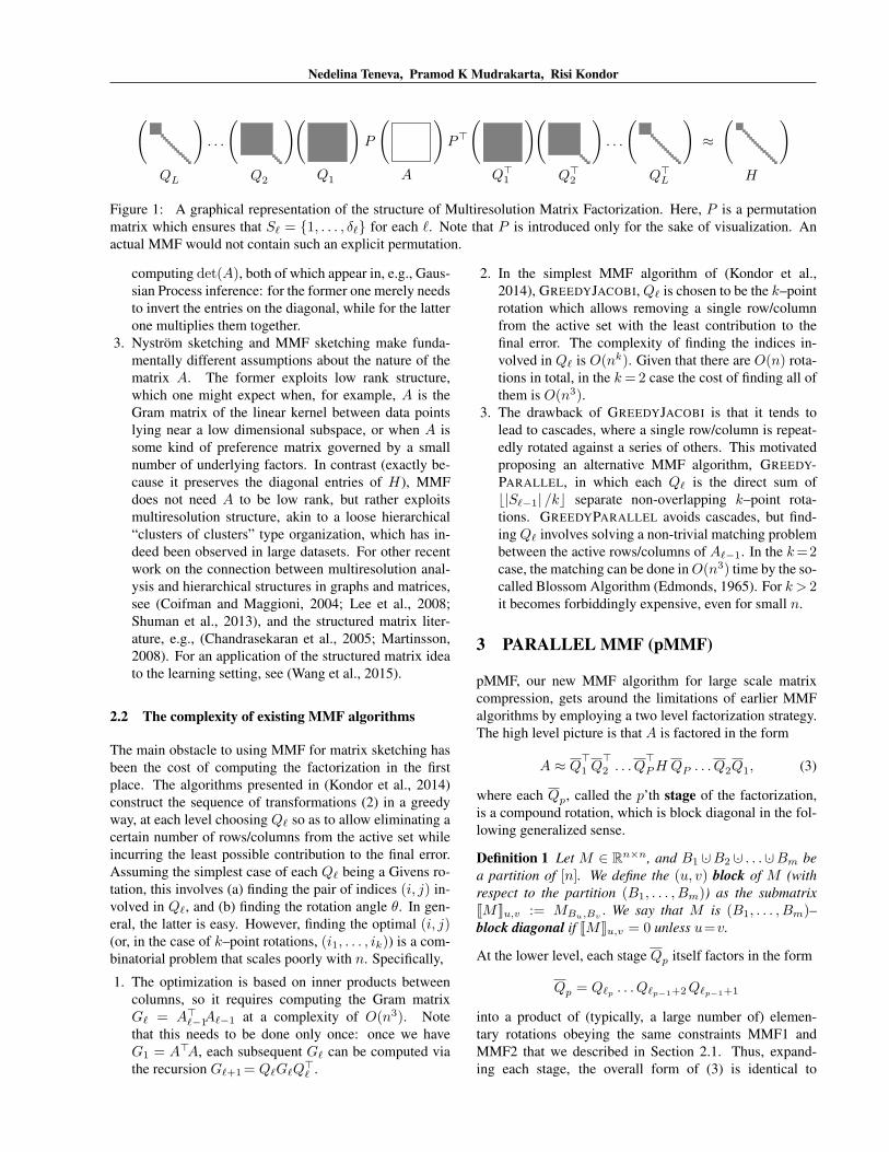
serial MMF pMMF operations pMMF time Nproc

dense sparse dense sparse dense sparseComputing Gram matrices n3 γn3 Pcn2 γPcn2 Pc3 γPc3 m2

Finding Rotations n3 n3 cn cn c2 c m

Updating Gram matrices n3 γ2n3 c2n γ2c2n c3 γ2c3 m

Applying rotations kn2 γkn2 kn2 γkn2 kc2 γkc2 m2

Clustering pmn2 γpmn2 pcn γpcn m2

Reblocking pn2 γpn2 pcn γpcn m

Factorization total n3 n3 Pcn2 γPcn2 Pc3 γPc3 m2

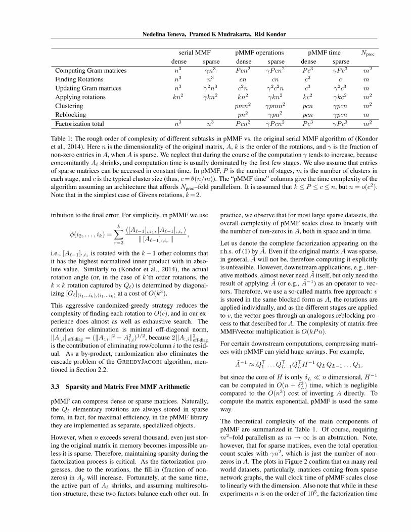
Table 1: The rough order of complexity of different subtasks in pMMF vs. the original serial MMF algorithm of (Kondoret al., 2014). Here n is the dimensionality of the original matrix, A, k is the order of the rotations, and γ is the fraction ofnon-zero entries in A, when A is sparse. We neglect that during the course of the computation γ tends to increase, becauseconcomitantly Aℓ shrinks, and computation time is usually dominated by the first few stages. We also assume that entriesof sparse matrices can be accessed in constant time. In pMMF, P is the number of stages, m is the number of clusters ineach stage, and c is the typical cluster size (thus, c= θ(n/m)). The “pMMF time” columns give the time complexity of thealgorithm assuming an architecture that affords Nproc–fold parallelism. It is assumed that k ≤ P ≤ c ≤ n, but n = o(c2).Note that in the simplest case of Givens rotations, k=2.

tribution to the final error. For simplicity, in pMMF we use

ϕ(i2, . . . , ik) =

k∑r=2

⟨[Aℓ−1]:,i1 , [Aℓ−1]:,ir ⟩∥ [Aℓ−1]:,ir ∥

,

i.e., [Aℓ−1]:,i1 is rotated with the k− 1 other columns thatit has the highest normalized inner product with in abso-lute value. Similarly to (Kondor et al., 2014), the actualrotation angle (or, in the case of k’th order rotations, thek×k rotation captured by Qℓ) is determined by diagonal-izing [Gℓ](i1...ik),(i1...ik) at a cost of O(k3).

This aggressive randomized-greedy strategy reduces thecomplexity of finding each rotation to O(c), and in our ex-perience does almost as well as exhaustive search. Thecriterion for elimination is minimal off-diagonal norm,∥A:,i∥off-diag = (∥A:,i∥2 − A2

i,i)1/2, because 2∥A:,i∥2off-diag

is the contribution of eliminating row/column i to the resid-ual. As a by-product, randomization also eliminates thecascade problem of the GREEDYJACOBI algorithm, men-tioned in Section 2.2.

3.3 Sparsity and Matrix Free MMF Arithmetic

pMMF can compress dense or sparse matrices. Naturally,the Qℓ elementary rotations are always stored in sparseform, in fact, for maximal efficiency, in the pMMF librarythey are implemented as separate, specialized objects.

However, when n exceeds several thousand, even just stor-ing the original matrix in memory becomes impossible un-less it is sparse. Therefore, maintaining sparsity during thefactorization process is critical. As the factorization pro-gresses, due to the rotations, the fill-in (fraction of non-zeros) in Ap will increase. Fortunately, at the same time,the active part of Aℓ shrinks, and assuming multiresolu-tion structure, these two factors balance each other out. In

practice, we observe that for most large sparse datasets, theoverall complexity of pMMF scales close to linearly withthe number of non-zeros in A, both in space and in time.

Let us denote the complete factorization appearing on ther.h.s. of (1) by A. Even if the original matrix A was sparse,in general, A will not be, therefore computing it explicitlyis unfeasible. However, downstream applications, e.g., iter-ative methods, almost never need A itself, but only need theresult of applying A (or e.g., A−1) as an operator to vec-tors. Therefore, we use a so-called matrix free approach: vis stored in the same blocked form as A, the rotations areapplied individually, and as the different stages are appliedto v, the vector goes through an analogous reblocking pro-cess to that described for A. The complexity of matrix-freeMMF/vector multiplication is O(kPn).

For certain downstream computations, compressing matri-ces with pMMF can yield huge savings. For example,

A−1 ≈ Q⊤1 . . . Q⊤

L−1Q⊤LH

−1 QLQL−1 . . . Q1,

but since the core of H is only δL ≪ n dimensional, H−1

can be computed in O(n + δ3L) time, which is negligiblecompared to the O(n3) cost of inverting A directly. Tocompute the matrix exponential, pMMF is used the sameway.

The theoretical complexity of the main components ofpMMF are summarized in Table 1. Of course, requiringm2–fold parallelism as m → ∞ is an abstraction. Note,however, that for sparse matrices, even the total operationcount scales with γn2, which is just the number of non-zeros in A. The plots in Figure 2 confirm that on many realworld datasets, particularly, matrices coming from sparsenetwork graphs, the wall clock time of pMMF scales closeto linearly with the dimension. Also note that while in theseexperiments n is on the order of 105, the factorization time

Multiresolution Matrix Compression

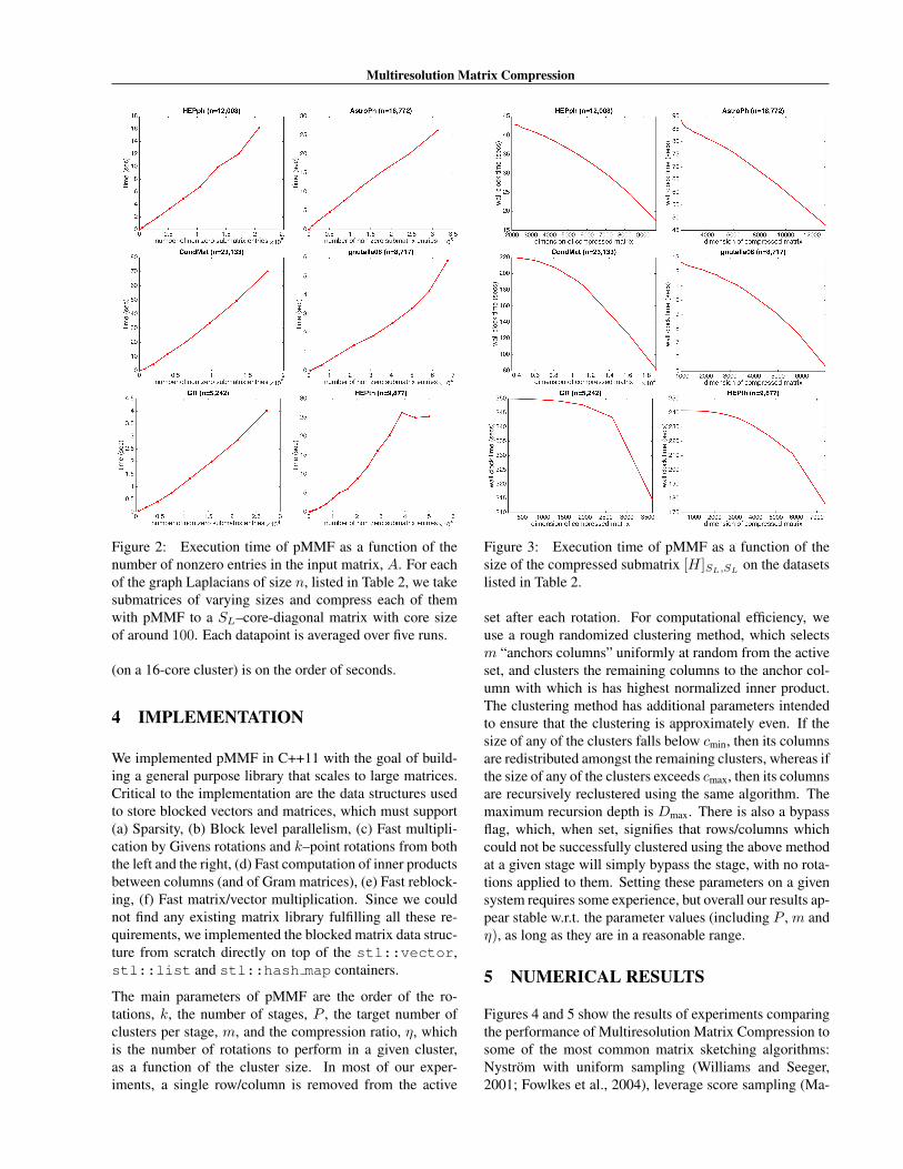
Figure 2: Execution time of pMMF as a function of thenumber of nonzero entries in the input matrix, A. For eachof the graph Laplacians of size n, listed in Table 2, we takesubmatrices of varying sizes and compress each of themwith pMMF to a SL–core-diagonal matrix with core sizeof around 100. Each datapoint is averaged over five runs.

(on a 16-core cluster) is on the order of seconds.

4 IMPLEMENTATION

We implemented pMMF in C++11 with the goal of build-ing a general purpose library that scales to large matrices.Critical to the implementation are the data structures usedto store blocked vectors and matrices, which must support(a) Sparsity, (b) Block level parallelism, (c) Fast multipli-cation by Givens rotations and k–point rotations from boththe left and the right, (d) Fast computation of inner productsbetween columns (and of Gram matrices), (e) Fast reblock-ing, (f) Fast matrix/vector multiplication. Since we couldnot find any existing matrix library fulfilling all these re-quirements, we implemented the blocked matrix data struc-ture from scratch directly on top of the stl::vector,stl::list and stl::hash map containers.

The main parameters of pMMF are the order of the ro-tations, k, the number of stages, P , the target number ofclusters per stage, m, and the compression ratio, η, whichis the number of rotations to perform in a given cluster,as a function of the cluster size. In most of our exper-iments, a single row/column is removed from the active

Figure 3: Execution time of pMMF as a function of thesize of the compressed submatrix [H]SL,SL

on the datasetslisted in Table 2.

set after each rotation. For computational efficiency, weuse a rough randomized clustering method, which selectsm “anchors columns” uniformly at random from the activeset, and clusters the remaining columns to the anchor col-umn with which is has highest normalized inner product.The clustering method has additional parameters intendedto ensure that the clustering is approximately even. If thesize of any of the clusters falls below cmin, then its columnsare redistributed amongst the remaining clusters, whereas ifthe size of any of the clusters exceeds cmax, then its columnsare recursively reclustered using the same algorithm. Themaximum recursion depth is Dmax. There is also a bypassflag, which, when set, signifies that rows/columns whichcould not be successfully clustered using the above methodat a given stage will simply bypass the stage, with no rota-tions applied to them. Setting these parameters on a givensystem requires some experience, but overall our results ap-pear stable w.r.t. the parameter values (including P , m andη), as long as they are in a reasonable range.

5 NUMERICAL RESULTS

Figures 4 and 5 show the results of experiments comparingthe performance of Multiresolution Matrix Compression tosome of the most common matrix sketching algorithms:Nystrom with uniform sampling (Williams and Seeger,2001; Fowlkes et al., 2004), leverage score sampling (Ma-

Nedelina Teneva, Pramod K Mudrakarta, Risi Kondor

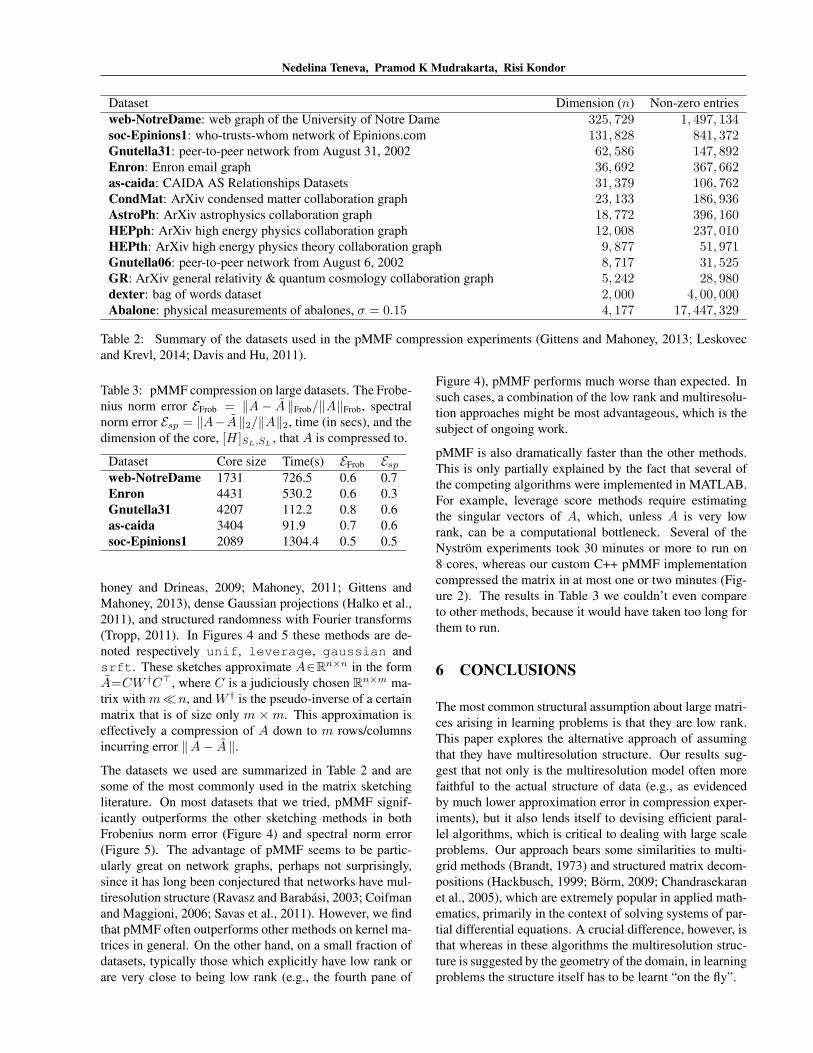
Dataset Dimension (n) Non-zero entriesweb-NotreDame: web graph of the University of Notre Dame 325, 729 1, 497, 134soc-Epinions1: who-trusts-whom network of Epinions.com 131, 828 841, 372Gnutella31: peer-to-peer network from August 31, 2002 62, 586 147, 892Enron: Enron email graph 36, 692 367, 662as-caida: CAIDA AS Relationships Datasets 31, 379 106, 762CondMat: ArXiv condensed matter collaboration graph 23, 133 186, 936AstroPh: ArXiv astrophysics collaboration graph 18, 772 396, 160HEPph: ArXiv high energy physics collaboration graph 12, 008 237, 010HEPth: ArXiv high energy physics theory collaboration graph 9, 877 51, 971Gnutella06: peer-to-peer network from August 6, 2002 8, 717 31, 525GR: ArXiv general relativity & quantum cosmology collaboration graph 5, 242 28, 980dexter: bag of words dataset 2, 000 4, 00, 000Abalone: physical measurements of abalones, σ = 0.15 4, 177 17, 447, 329

Table 2: Summary of the datasets used in the pMMF compression experiments (Gittens and Mahoney, 2013; Leskovecand Krevl, 2014; Davis and Hu, 2011).

Table 3: pMMF compression on large datasets. The Frobe-nius norm error EFrob = ∥A− A ∥Frob/∥A∥Frob, spectralnorm error Esp = ∥A− A ∥2/∥A∥2, time (in secs), and thedimension of the core, [H]SL,SL , that A is compressed to.

Dataset Core size Time(s) EFrob Espweb-NotreDame 1731 726.5 0.6 0.7Enron 4431 530.2 0.6 0.3Gnutella31 4207 112.2 0.8 0.6as-caida 3404 91.9 0.7 0.6soc-Epinions1 2089 1304.4 0.5 0.5

honey and Drineas, 2009; Mahoney, 2011; Gittens andMahoney, 2013), dense Gaussian projections (Halko et al.,2011), and structured randomness with Fourier transforms(Tropp, 2011). In Figures 4 and 5 these methods are de-noted respectively unif, leverage, gaussian andsrft. These sketches approximate A∈Rn×n in the formA=CW †C⊤, where C is a judiciously chosen Rn×m ma-trix with m≪n, and W † is the pseudo-inverse of a certainmatrix that is of size only m × m. This approximation iseffectively a compression of A down to m rows/columnsincurring error ∥A− A ∥.

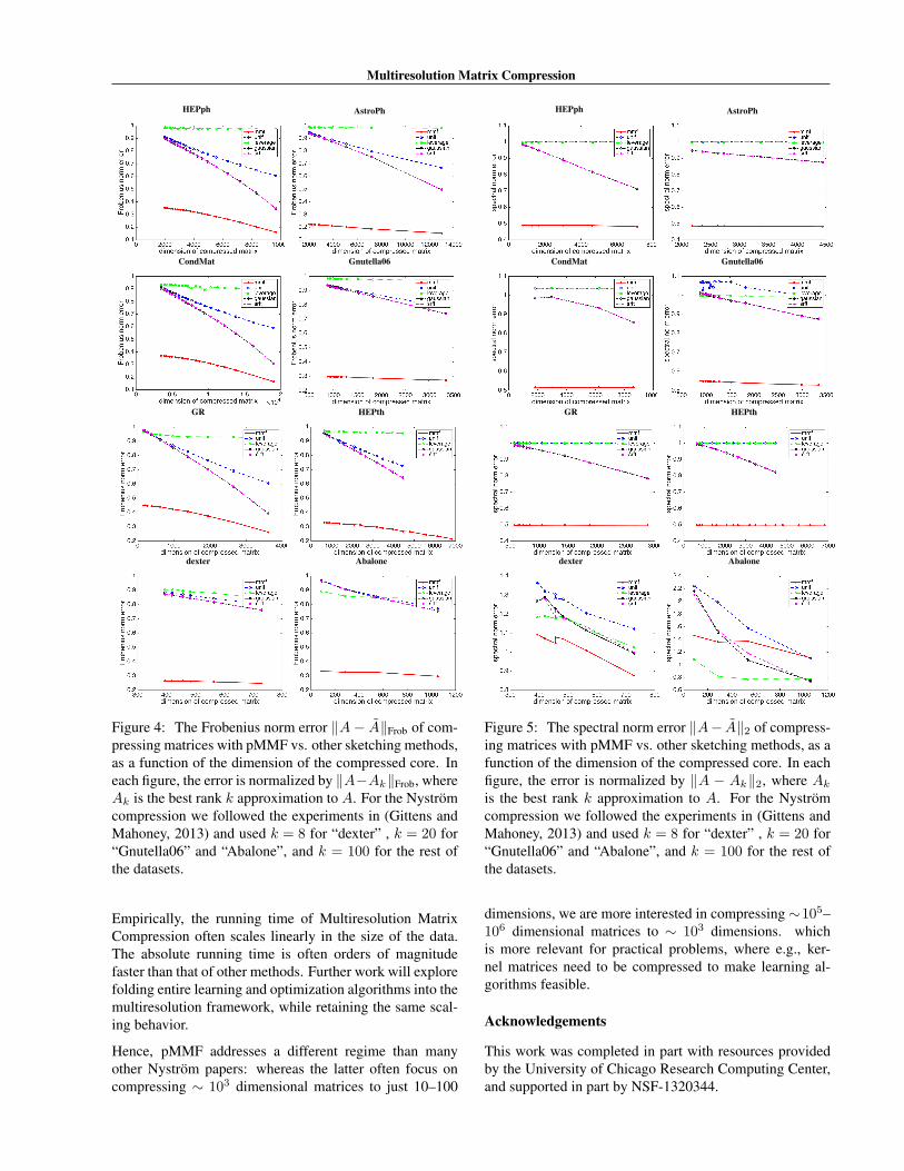
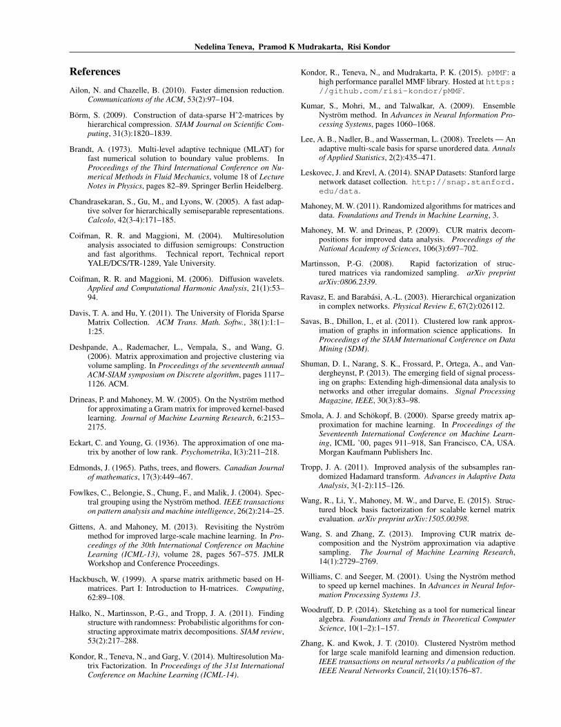
The datasets we used are summarized in Table 2 and aresome of the most commonly used in the matrix sketchingliterature. On most datasets that we tried, pMMF signif-icantly outperforms the other sketching methods in bothFrobenius norm error (Figure 4) and spectral norm error(Figure 5). The advantage of pMMF seems to be partic-ularly great on network graphs, perhaps not surprisingly,since it has long been conjectured that networks have mul-tiresolution structure (Ravasz and Barabasi, 2003; Coifmanand Maggioni, 2006; Savas et al., 2011). However, we findthat pMMF often outperforms other methods on kernel ma-trices in general. On the other hand, on a small fraction ofdatasets, typically those which explicitly have low rank orare very close to being low rank (e.g., the fourth pane of

Figure 4), pMMF performs much worse than expected. Insuch cases, a combination of the low rank and multiresolu-tion approaches might be most advantageous, which is thesubject of ongoing work.

pMMF is also dramatically faster than the other methods.This is only partially explained by the fact that several ofthe competing algorithms were implemented in MATLAB.For example, leverage score methods require estimatingthe singular vectors of A, which, unless A is very lowrank, can be a computational bottleneck. Several of theNystrom experiments took 30 minutes or more to run on8 cores, whereas our custom C++ pMMF implementationcompressed the matrix in at most one or two minutes (Fig-ure 2). The results in Table 3 we couldn’t even compareto other methods, because it would have taken too long forthem to run.

6 CONCLUSIONS

The most common structural assumption about large matri-ces arising in learning problems is that they are low rank.This paper explores the alternative approach of assumingthat they have multiresolution structure. Our results sug-gest that not only is the multiresolution model often morefaithful to the actual structure of data (e.g., as evidencedby much lower approximation error in compression exper-iments), but it also lends itself to devising efficient paral-lel algorithms, which is critical to dealing with large scaleproblems. Our approach bears some similarities to multi-grid methods (Brandt, 1973) and structured matrix decom-positions (Hackbusch, 1999; Borm, 2009; Chandrasekaranet al., 2005), which are extremely popular in applied math-ematics, primarily in the context of solving systems of par-tial differential equations. A crucial difference, however, isthat whereas in these algorithms the multiresolution struc-ture is suggested by the geometry of the domain, in learningproblems the structure itself has to be learnt “on the fly”.

Multiresolution Matrix Compression

HEPph AstroPh

CondMat Gnutella06

GR HEPth

dexter Abalone

Figure 4: The Frobenius norm error ∥A− A∥Frob of com-pressing matrices with pMMF vs. other sketching methods,as a function of the dimension of the compressed core. Ineach figure, the error is normalized by ∥A−Ak∥Frob, whereAk is the best rank k approximation to A. For the Nystromcompression we followed the experiments in (Gittens andMahoney, 2013) and used k = 8 for “dexter” , k = 20 for“Gnutella06” and “Abalone”, and k = 100 for the rest ofthe datasets.

Empirically, the running time of Multiresolution MatrixCompression often scales linearly in the size of the data.The absolute running time is often orders of magnitudefaster than that of other methods. Further work will explorefolding entire learning and optimization algorithms into themultiresolution framework, while retaining the same scal-ing behavior.

Hence, pMMF addresses a different regime than manyother Nystrom papers: whereas the latter often focus oncompressing ∼ 103 dimensional matrices to just 10–100

HEPph AstroPh

CondMat Gnutella06

GR HEPth

dexter Abalone

Figure 5: The spectral norm error ∥A− A∥2 of compress-ing matrices with pMMF vs. other sketching methods, as afunction of the dimension of the compressed core. In eachfigure, the error is normalized by ∥A − Ak∥2, where Ak

is the best rank k approximation to A. For the Nystromcompression we followed the experiments in (Gittens andMahoney, 2013) and used k = 8 for “dexter” , k = 20 for“Gnutella06” and “Abalone”, and k = 100 for the rest ofthe datasets.

dimensions, we are more interested in compressing ∼105–106 dimensional matrices to ∼ 103 dimensions. whichis more relevant for practical problems, where e.g., ker-nel matrices need to be compressed to make learning al-gorithms feasible.

Acknowledgements

This work was completed in part with resources providedby the University of Chicago Research Computing Center,and supported in part by NSF-1320344.

Nedelina Teneva, Pramod K Mudrakarta, Risi Kondor

ReferencesAilon, N. and Chazelle, B. (2010). Faster dimension reduction.

Communications of the ACM, 53(2):97–104.

Borm, S. (2009). Construction of data-sparse Hˆ2-matrices byhierarchical compression. SIAM Journal on Scientific Com-puting, 31(3):1820–1839.

Brandt, A. (1973). Multi-level adaptive technique (MLAT) forfast numerical solution to boundary value problems. InProceedings of the Third International Conference on Nu-merical Methods in Fluid Mechanics, volume 18 of LectureNotes in Physics, pages 82–89. Springer Berlin Heidelberg.

Chandrasekaran, S., Gu, M., and Lyons, W. (2005). A fast adap-tive solver for hierarchically semiseparable representations.Calcolo, 42(3-4):171–185.

Coifman, R. R. and Maggioni, M. (2004). Multiresolutionanalysis associated to diffusion semigroups: Constructionand fast algorithms. Technical report, Technical reportYALE/DCS/TR-1289, Yale University.

Coifman, R. R. and Maggioni, M. (2006). Diffusion wavelets.Applied and Computational Harmonic Analysis, 21(1):53–94.

Davis, T. A. and Hu, Y. (2011). The University of Florida SparseMatrix Collection. ACM Trans. Math. Softw., 38(1):1:1–1:25.

Deshpande, A., Rademacher, L., Vempala, S., and Wang, G.(2006). Matrix approximation and projective clustering viavolume sampling. In Proceedings of the seventeenth annualACM-SIAM symposium on Discrete algorithm, pages 1117–1126. ACM.

Drineas, P. and Mahoney, M. W. (2005). On the Nystrom methodfor approximating a Gram matrix for improved kernel-basedlearning. Journal of Machine Learning Research, 6:2153–2175.

Eckart, C. and Young, G. (1936). The approximation of one ma-trix by another of low rank. Psychometrika, I(3):211–218.

Edmonds, J. (1965). Paths, trees, and flowers. Canadian Journalof mathematics, 17(3):449–467.

Fowlkes, C., Belongie, S., Chung, F., and Malik, J. (2004). Spec-tral grouping using the Nystrom method. IEEE transactionson pattern analysis and machine intelligence, 26(2):214–25.

Gittens, A. and Mahoney, M. (2013). Revisiting the Nystrommethod for improved large-scale machine learning. In Pro-ceedings of the 30th International Conference on MachineLearning (ICML-13), volume 28, pages 567–575. JMLRWorkshop and Conference Proceedings.

Hackbusch, W. (1999). A sparse matrix arithmetic based on H-matrices. Part I: Introduction to H-matrices. Computing,62:89–108.

Halko, N., Martinsson, P.-G., and Tropp, J. A. (2011). Findingstructure with randomness: Probabilistic algorithms for con-structing approximate matrix decompositions. SIAM review,53(2):217–288.

Kondor, R., Teneva, N., and Garg, V. (2014). Multiresolution Ma-trix Factorization. In Proceedings of the 31st InternationalConference on Machine Learning (ICML-14).

Kondor, R., Teneva, N., and Mudrakarta, P. K. (2015). pMMF: ahigh performance parallel MMF library. Hosted at https://github.com/risi-kondor/pMMF.

Kumar, S., Mohri, M., and Talwalkar, A. (2009). EnsembleNystrom method. In Advances in Neural Information Pro-cessing Systems, pages 1060–1068.

Lee, A. B., Nadler, B., and Wasserman, L. (2008). Treelets — Anadaptive multi-scale basis for sparse unordered data. Annalsof Applied Statistics, 2(2):435–471.

Leskovec, J. and Krevl, A. (2014). SNAP Datasets: Stanford largenetwork dataset collection. http://snap.stanford.edu/data.

Mahoney, M. W. (2011). Randomized algorithms for matrices anddata. Foundations and Trends in Machine Learning, 3.

Mahoney, M. W. and Drineas, P. (2009). CUR matrix decom-positions for improved data analysis. Proceedings of theNational Academy of Sciences, 106(3):697–702.

Martinsson, P.-G. (2008). Rapid factorization of struc-tured matrices via randomized sampling. arXiv preprintarXiv:0806.2339.

Ravasz, E. and Barabasi, A.-L. (2003). Hierarchical organizationin complex networks. Physical Review E, 67(2):026112.

Savas, B., Dhillon, I., et al. (2011). Clustered low rank approx-imation of graphs in information science applications. InProceedings of the SIAM International Conference on DataMining (SDM).

Shuman, D. I., Narang, S. K., Frossard, P., Ortega, A., and Van-dergheynst, P. (2013). The emerging field of signal process-ing on graphs: Extending high-dimensional data analysis tonetworks and other irregular domains. Signal ProcessingMagazine, IEEE, 30(3):83–98.

Smola, A. J. and Schokopf, B. (2000). Sparse greedy matrix ap-proximation for machine learning. In Proceedings of theSeventeenth International Conference on Machine Learn-ing, ICML ’00, pages 911–918, San Francisco, CA, USA.Morgan Kaufmann Publishers Inc.

Tropp, J. A. (2011). Improved analysis of the subsamples ran-domized Hadamard transform. Advances in Adaptive DataAnalysis, 3(1-2):115–126.

Wang, R., Li, Y., Mahoney, M. W., and Darve, E. (2015). Struc-tured block basis factorization for scalable kernel matrixevaluation. arXiv preprint arXiv:1505.00398.

Wang, S. and Zhang, Z. (2013). Improving CUR matrix de-composition and the Nystrom approximation via adaptivesampling. The Journal of Machine Learning Research,14(1):2729–2769.

Williams, C. and Seeger, M. (2001). Using the Nystrom methodto speed up kernel machines. In Advances in Neural Infor-mation Processing Systems 13.

Woodruff, D. P. (2014). Sketching as a tool for numerical linearalgebra. Foundations and Trends in Theoretical ComputerScience, 10(1–2):1–157.

Zhang, K. and Kwok, J. T. (2010). Clustered Nystrom methodfor large scale manifold learning and dimension reduction.IEEE transactions on neural networks / a publication of theIEEE Neural Networks Council, 21(10):1576–87.