MULTIRESOLUTION ANALYSIS FOR 2D TURBULENCE…pfischer/Publications_files/3.pdf · MULTIRESOLUTION...

DISCRETE AND CONTINUOUS Website: http://AIMsciences.orgDYNAMICAL SYSTEMS–SERIES BVolume 7, Number 4, June 2007 pp. 717–734

MULTIRESOLUTION ANALYSIS FOR 2D TURBULENCE.

PART 2: A PHYSICAL INTERPRETATION

Patrick Fischer, Charles-Henri Bruneau

Universite Bordeaux 1, IMB, CNRS UMR 5466, INRIA projet MC2,351, Cours de la Liberation, 33405 Talence Cedex, France

Hamid KellayUniversite Bordeaux1, CPMOH, CNRS UMR 5798,

351, Cours de la Liberation, 33405 Talence Cedex, France

(Communicated by Ka-Kit Tung)

Abstract. Multiresolution methods such as the wavelet packets or the cosinepackets are more and more used in physical applications and in particular intwo-dimensional turbulence. The numerical results of the first part of thispaper have shown that the wavelet packets decomposition is well suited forstudying this kind of problem: the visualization of the vorticity field is better,without any artefacts, than the visualization with the cosine packets filtering.The current second part of the paper is devoted to the physical interpretationof the filtered fields obtained in the first part. Energy and enstrophy spectraas well as energy and enstrophy fluxes are computed to determine the role ofeach filtered field with respect to the cascades.

1. Introduction. It has been shown in the first part of this paper [3] that thewavelet packets filtering can be successfully used for analyzing two-dimensionalturbulence. This technique allows the separation of two structures: the solid rota-tion part of the vortices and the remaining mainly composed of vorticity filaments.The wavelet packets filtering leads to continuous filtered fields and avoids the dis-continuities that would be created by a direct cut-off filtering. The spurious effectsdue to this kind of discontinuities created by a direct filtering have been discussedin [4]. It has been shown in particular in that paper that the discontinuities areresponsible for the creation of spurious coefficients in Fourier space that alter thecorresponding energy and enstrophy spectra.In the present paper we will refine the explanations given in the first part and de-tail the physical interpretation of the filtered fields given in [1]. The energy andenstrophy fluxes will be computed and they will allow a better understanding of theenergy and enstrophy transfer processes through the scales. A few results aboutthe pressure field and its correlation to the solid rotations field will be also given inthe paper.The paper is organized as follows. The theoretical background is recalled in section2 where we make some remarks about the Danilov inequality. The experimentalsetup and the filtering process are described in section 3. Direct numerical simula-tions are used to obtain a two-dimensional turbulent flow at relatively high Reynolds

2000 Mathematics Subject Classification. 65T60,76F65.Key words and phrases. Wavelets, 2D turbulence.

717

718 P. FISCHER, CH.-H BRUNEAU AND H. KELLAY

numbers. The filtering algorithm leading to continuous filtered fields is describedbut the theory of wavelet packets is not recalled here. The results about the energyand enstrophy fluxes are given in section 4. It is shown that two-dimensional turbu-lence admits two distinct structures: vortical structures and filamentary structures.The first ones are responsible for the inverse transfers of energy while the secondones are responsible for the forward transfer of enstrophy. The decomposition ofthe nonlinear term in the Navier-Stokes equation is described in section 5. This de-composition permits the separation of the energy or enstrophy transport due to thesolid rotations from the transport due to the filaments. Conclusions and remarksare given in section 6.

2. Theoretical background. Two-dimensional turbulence, in a finite but peri-odic domain, is governed by two invariants, the energy and the enstrophy. Themean energy per unit mass E is defined by,

E ≡

⟨1

2|v|2

⟩=

1

2

1

S(BL)

∫

BL

|v(x)|2dx (1)

where BL denotes the physical domain and S(BL) its corresponding surface. If oneconsiders now the velocity v as a L-periodic function, it can be decomposed as aFourier series:

v(x) =∑

k

v(k)e2iπ

Lk.x, k ∈ Z

2. (2)

The low-pass filtered velocity function is then defined as,

v<K(x) =

∑

|k|≤K

v(k)e2iπ

Lk.x (3)

and the high-pass filtered velocity function as:

v>K(x) =

∑

|k|>K

v(k)e2iπ

Lk.x. (4)

This decomposition of the velocity,

v(x) = v<K(x) + v

>K(x), (5)

was used for the first time by Obukhov [11], [12]. Introducing this splitting inthe Navier-Stokes equations, one obtain a scale-by-scale energy budget equationdescribed by Frisch [5]:

∂tE(K) + ΠE(K) = DE(K) + FE(K). (6)

where

E(K) ≡

⟨1

2|v<

K |2⟩

=1

2

∑

|k|≤K

|v(k)|2, (7)

denotes the cumulative energy, ΠE(K) the energy flux due to the nonlinear termsthrough the wavenumber K, DE(K) the energy dissipation, and FE(K) the energyinjection. The energy spectrum is then defined by,

E(k) ≡dE(k)

dk, (8)

and the total energy can be rewritten as,

E =

∫ ∞

0

E(k)dk. (9)

MULTIRESOLUTION ANALYSIS FOR 2D TURBULENCE. PART 2 719

The same splitting can be used in the Navier-Stokes equation written for the vor-ticity and a scale-by-scale enstrophy budget equation can be obtained:

∂tZ(K) + ΠZ(K) = DZ(K) + FZ(K), (10)

where Z(K) denotes the cumulative enstrophy, ΠZ(K) the enstrophy flux, DZ(K)the enstrophy dissipation, and FZ(K) the enstrophy injection. The enstrophy Z

can be defined in the same way as the energy,

Z ≡

⟨1

2|ω|2

⟩=

1

2

1

S(BL)

∫

BL

|ω(x)|2dx, (11)

where ω = ∇× v is the vorticity field. The relation between the enstrophy and theenstrophy spectrum is then given by:

Z =

∫ ∞

0

Z(k)dk (12)

where Z(k) stands for the enstrophy spectrum. The energy and enstrophy spectraare linked to each other in Fourier space by the following relation:

Z(k) =

(2πk

L

)2

E(k) (13)

which reduces toZ(k) = k2E(k) (14)

in a 2π-periodic bounded domain. Using the same notation as Tung and Gkioulekasin [16] this relation can be written in a more general form:

Z(k) = Λ(k)E(k). (15)

The fluxes are also related to each other by the same kind of relation:

∂ΠZ(k)

∂k= Λ(k)

∂ΠE(k)

∂k. (16)

Outside the forcing range, the fluxes should verify the following Danilov inequality:

Λ(k)ΠE(k) < ΠZ(k). (17)

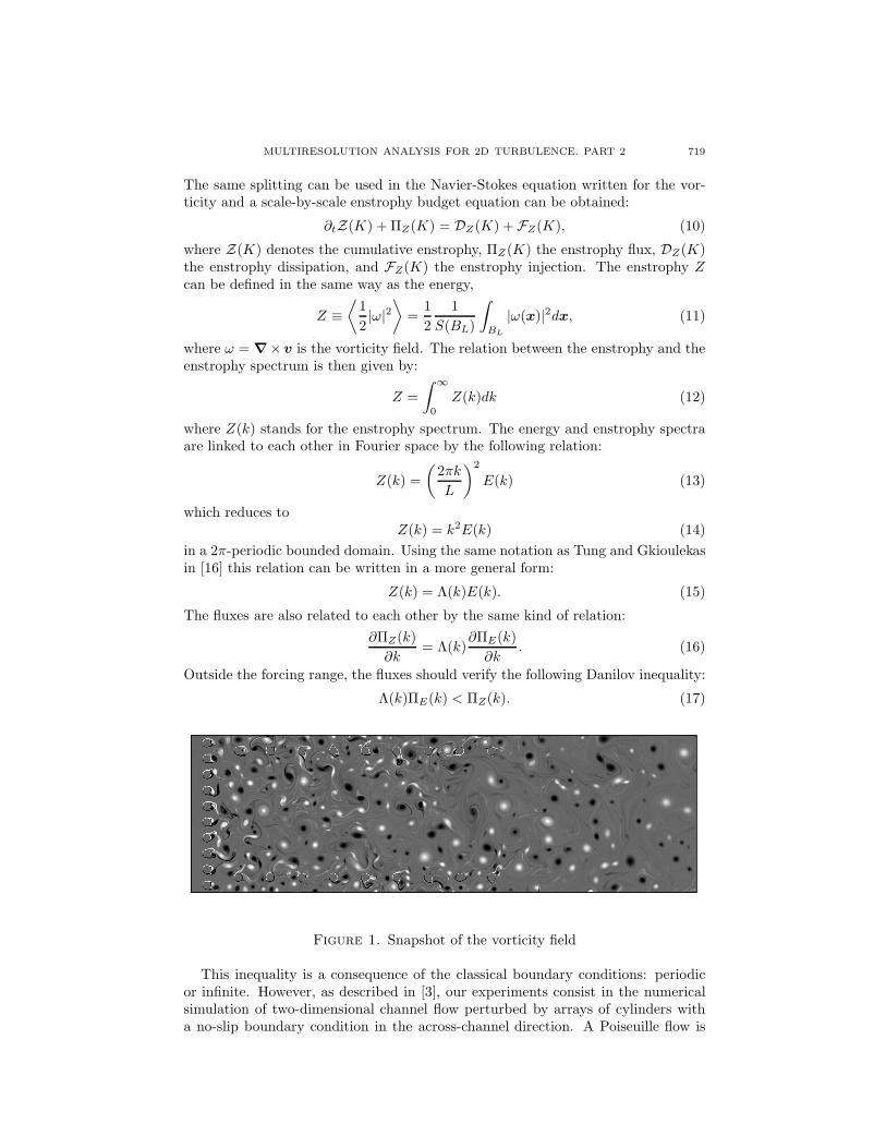
Figure 1. Snapshot of the vorticity field

This inequality is a consequence of the classical boundary conditions: periodicor infinite. However, as described in [3], our experiments consist in the numericalsimulation of two-dimensional channel flow perturbed by arrays of cylinders witha no-slip boundary condition in the across-channel direction. A Poiseuille flow is


imposed on the entrance section of the channel, and a non reflecting condition isimposed on the exit section. The numerical experiments give a realistic picture ofa fluid entering in a channel, pertubated by cylindrical obstacles and exiting thechannel. These simulations describe the behavior of a shallow river or a real soapfilm experiment like in [9, 10, 14, 13]. The spectra are computed in a selected squarelocated at the end of the channel. Thus we do not have any periodic condition inany case, and the relations described above between the energy and the enstrophyspectra do not hold anymore. It has been shown in [4] that the energy-enstrophyrelation numerically diverges in our particular case. This relation is verified only fora short range of frequencies in the middle part of the spectra, approximately betweenk ≈ 3 and k ≈ 20. A detailed study has been performed, and the results have shownthat a Windowed Fourier Transform has to be used for the spectra computationsin order to remove the discontinuities created by the boundary conditions.

3. The experimental setup and the filtering process.

3.1. Experimental setup. In the first part [3], two numerical experiments, calledsimulation I and II, had been performed. Slightly different versions of simulation

II are considered in this paper. The additional cylinders along the channel are usedto increase the number of merging events, and thus to enhance the inverse energycascade phenomenon. In the first part, the energy injection scale kinj had beenconsidered to be equal to the diameter of the five big cylinders (kinj ≈ 10). Butit is a matter of fact that the small cylinders along the sides of the channel inducea second small energy injection around k = 20. So the energy injection shouldbe considered to lie between 10 and 20. In order to get a better localized energyinjection, the five big cylinders have been replaced by ten small cylinders. Fromnow, all the obstacles have the same diameter and induce the same energy injectionscale. The Reynolds number based on the cylinders diameter is Re = 50000 that islarge enough to get a fully developed turbulent flow. This is about the same valueas those used in soap film experiments [2, 9, 10]. A snapshot of the vorticity fieldfrom the upstream cylinders to the end of the channel is given in Figure 1

The simulations have been performed on a 640×2560 grid and the averages havebeen computed with 25 snapshots. A Tukey window with the parameter equal to0.1 has been used in all the computations in order to remove the discontinuitiescreated by the boundary conditions.

3.2. The filtering process. The theory concerning the wavelet packets has beendetailed in [3] and will not be repeated here. The same Daubechies type waveletsare used in the current paper to build the packets array, and the entropy criterion isused in the best basis selection process. In [3], a few tests were performed in orderto get the best wavelet mother, and to determine the number of scales necessaryfor an efficient representation of the flow. The criterion was then the minimizationof the entropy. It had been shown that it was not necessary to perform the waveletpackets decomposition over more than 3 scales when the finest scale corresponds toa 320 × 1280 grid. It has to be reminded that the scale sequence goes from finestscales to coarsest scales. It leads to the most efficient representation according tothe entropy criterion but not to the smoothest fields after filtering. It has beenshown in [4] that, as long as one is concerned with smoothing the discontinuities,it is necessary to go over at least 4 scales (for a finest scale corresponding to a320 × 1280 grid). That means that in [3], where only 3 scales were considered,


100

101

102

10−15

10−10

10−5

100

Total energy EFiltered energy E

sFiltered energy E

f

Slope k−2

Slope k−5.5

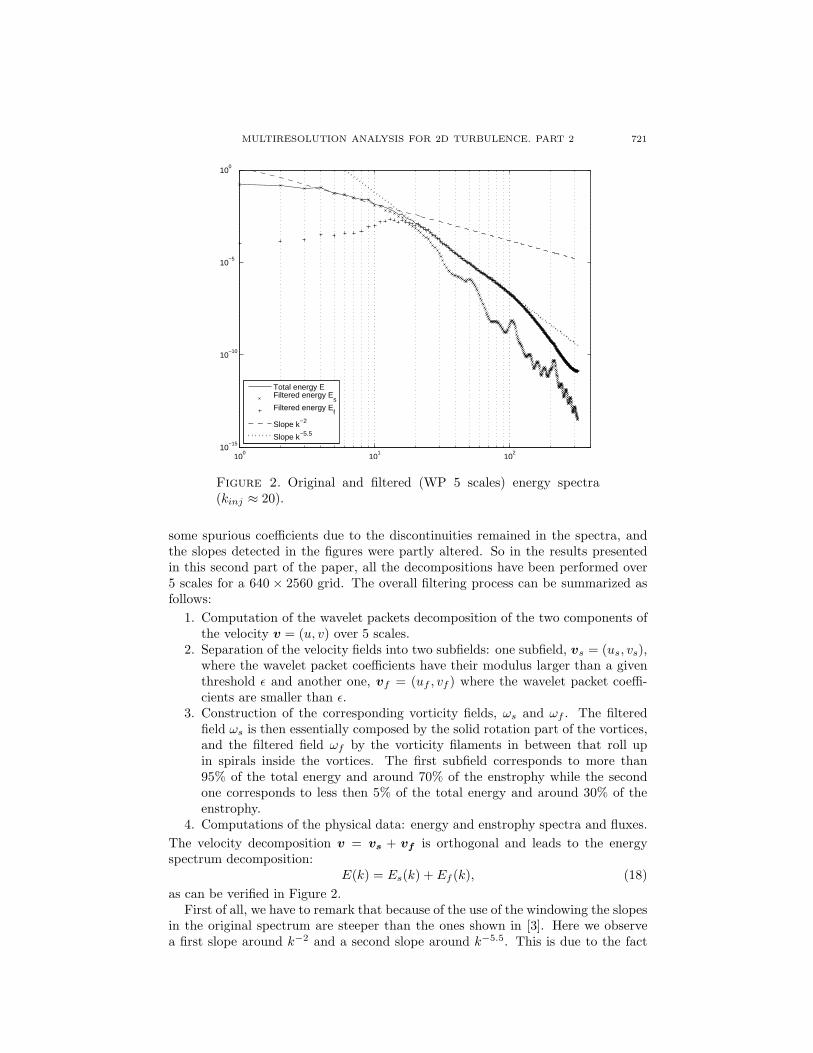
Figure 2. Original and filtered (WP 5 scales) energy spectra(kinj ≈ 20).

some spurious coefficients due to the discontinuities remained in the spectra, andthe slopes detected in the figures were partly altered. So in the results presentedin this second part of the paper, all the decompositions have been performed over5 scales for a 640 × 2560 grid. The overall filtering process can be summarized asfollows:

1. Computation of the wavelet packets decomposition of the two components ofthe velocity v = (u, v) over 5 scales.

2. Separation of the velocity fields into two subfields: one subfield, vs = (us, vs),where the wavelet packet coefficients have their modulus larger than a giventhreshold ǫ and another one, vf = (uf , vf ) where the wavelet packet coeffi-cients are smaller than ǫ.

3. Construction of the corresponding vorticity fields, ωs and ωf . The filteredfield ωs is then essentially composed by the solid rotation part of the vortices,and the filtered field ωf by the vorticity filaments in between that roll upin spirals inside the vortices. The first subfield corresponds to more than95% of the total energy and around 70% of the enstrophy while the secondone corresponds to less then 5% of the total energy and around 30% of theenstrophy.

4. Computations of the physical data: energy and enstrophy spectra and fluxes.

The velocity decomposition v = vs + vf is orthogonal and leads to the energyspectrum decomposition:

E(k) = Es(k) + Ef (k), (18)

as can be verified in Figure 2.First of all, we have to remark that because of the use of the windowing the slopes

in the original spectrum are steeper than the ones shown in [3]. Here we observea first slope around k−2 and a second slope around k−5.5. This is due to the fact


100

101

102

10−10

10−8

10−6

10−4

10−2

100

102

Total enstrophy ZFiltered enstrophy Z

sFiltered enstrophy Z

f

Slope k1/3

Slope k−3.5

Figure 3. Original and filtered (WP 5 scales) enstrophy spectra(kinj ≈ 20).

that all the spurious coefficients due to the discontinuities have been removed. Onecan then notice that both components are multiscale, although the part with thevortices dominates at low wavenumbers and the part mainly composed by filamentsdominates at high wavenumbers. The first slope is not really clear but the secondone is evident. These slopes and this decomposition can be also observed on theenstrophy spectra given in Figure 3.

It has been shown in [4] that the relation (15) with Λ(k) = 4π2k2 between theenergy and the enstrophy spectra is verified only in the middle part of the spectra(which is the significant part for k in the range 4 to 120 on both sides of the injectionscale kinj) due to the boundary conditions.

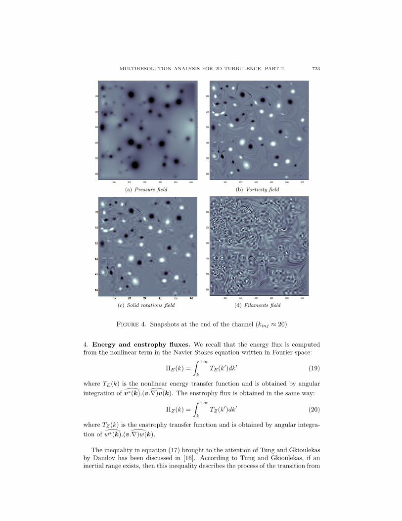
Remark: The pressure field is rarely studied in papers on two-dimensional tur-bulence but nevertheless can bring interesting information about the fluid. A snap-shot of the end of the pressure field is given in Figure 4.

The pressure field can be compared to the corresponding vorticity field. Thedecomposition into the two subfields obtained by the filtering process is also givenin Figure 4.

As can be easily observed, the peaks of the pressure correspond exactly to vor-ticity peaks. They correspond obviously to the solid rotation structures, and it canbe expected that the pressure spectrum should present the same behavior as thesolid rotations spectrum. Both spectra are given in Figure 5 and the similaritybetween the shape of the pressure spectrum and the shape of the solid rotationsenergy spectrum is clear.


100 200 300 400 500 600

100

200

300

400

500

600

(a) Pressure field

100 200 300 400 500 600

100

200

300

400

500

600

(b) Vorticity field

(c) Solid rotations field

100 200 300 400 500 600

100

200

300

400

500

600

(d) Filaments field

Figure 4. Snapshots at the end of the channel (kinj ≈ 20)

4. Energy and enstrophy fluxes. We recall that the energy flux is computedfrom the nonlinear term in the Navier-Stokes equation written in Fourier space:

ΠE(k) =

∫ +∞

k

TE(k′)dk′ (19)

where TE(k) is the nonlinear energy transfer function and is obtained by angular

integration of v∗(k). (v.∇)v(k). The enstrophy flux is obtained in the same way:

ΠZ(k) =

∫ +∞

k

TZ(k′)dk′ (20)

where TZ(k) is the enstrophy transfer function and is obtained by angular integra-

tion of w∗(k). (v.∇)w(k).

The inequality in equation (17) brought to the attention of Tung and Gkioulekasby Danilov has been discussed in [16]. According to Tung and Gkioulekas, if aninertial range exists, then this inequality describes the process of the transition from


100

101

102

10−14

10−12

10−10

10−8

10−6

10−4

10−2

100

Solid rotationsPressure

Figure 5. Pressure and solid rotations spectra (kinj ≈ 20).

100

101

102

−400

−200

0

200

400

600

800

ΠZ − Λ . Π

E

Figure 6. ΠZ − ΛΠE allowing to verify the Danilov inequality.


the leading cascade to the subleading cascade observed in the energy spectrum. Ascan be noticed in Figure 6, this inequality is verified almost everywhere exceptin a small range at large scales. It is not surprising since the inertial range doesnot stretch out on large scales. It has been mentionned by Tran in [15] that thebehavior at large scales of a fluid in an elongated and doubly periodic domain is farfrom understood. He describes in that paper how the inverse energy cascade can bepartially stopped. Furthermore in our case, the boundary conditions are differentand the fluid dynamics at large scale is very hard to predict. However, it can benoticed that the inequality is verified around k = 20 which is supposed to be theinjection scale.

100

101

102

−0.5

−0.4

−0.3

−0.2

−0.1

0

0.1

0.2

Π

E

ΠEs → s

ΠEf → f

Figure 7. Energy fluxes of the whole flow and of the separatestructures (kinj ≈ 20).

Let us now study the energy and enstrophy fluxes themselves. The energy andenstrophy fluxes corresponding to those experiments are respectively given in Fig-ure 7 and 8. The energy flux is negative for wavenumbers k below the injectionscale 20 and slightly positive but almost zero above. The enstrophy flux is on theother hand positive above the injection scale, and negative below. The zero crossingcorresponds approximately to the injection scale. These results show the existenceof leading cascades, upscales for the inverse energy cascade and downscales for thedirect enstrophy cascade but also the existence of subleading cascades as theoreti-cally shown by Tung and Gkioulekas in [6, 7] and [16]. It can also be noticed thatthe injection scale being relatively large, the energy cascade cannot be developedcompletely. A priori and if the turbulence is inertial, the energy flux should presenta plateau in the small wavenumber range. Our simulations do not produce a largeplateau but an explanation for this is the limitation of the range of scales probed


and the presence of the boundaries. In our mathematical model, we did not useany artificial dissipation term like an hyper or hypoviscosity terms, and the twocascades could certainly be improved by using artificial dissipation terms at largeand small scales.

Finally, even if our experiment does not verify the usual boundary conditions ofthe 2D turbulence theory, both the energy flux and the enstrophy flux show thatthe classical picture of 2D turbulence, i.e. coexistence of two cascades, is valid forthe flow considered here regardless of whether a plateau for the energy flux or en-strophy flux is achieved.

4.1. Fluxes for the filtered fields. In order to study, in detail, the energy trans-fer, we focus now on the nonlinear energy transfer function which, due to the or-thogonal decomposition, can be written as:

TE(k) = v∗(k). (v.∇)v(k)

= vs∗(k). (v.∇)vs(k) + vs

∗(k). (v.∇)vf (k) (21)

+ vf∗(k). (v.∇)vs(k) + vf

∗(k). (v.∇)vf (k).

The global energy transfer can be split into four parts corresponding to themultiscale transfers from one subfield to itself or to the other one. For instance,

vs∗(k). (v.∇)vf (k) is the energy transfer from the vorticity filaments subfield to the

solid rotation subfield. The fluxes corresponding to each term in the expression for

the total energy transfer function will be denoted as for example Πf→sE which is the

flux corresponding to the transfer term previously described. In the same way, thenonlinear enstrophy transfer term is also split into four parts:

TZ(k) = ω∗(k). (v.∇)ω(k)

= ω∗s(k). (v.∇)ωs(k) + ω∗

s(k). (v.∇)ωf (k) (22)

+ ω∗f (k). (v.∇)ωs(k) + ω∗

f (k). (v.∇)ωf (k).

Using these decompositions, the fluxes associated with each structure as well as thefluxes associated with the interactions of the two structures can be obtained. Letus first consider the energy fluxes of the whole flow and of the separate structuresin Figure 7.

The energy flux for the vortices shows a large negative part at small k which issimilar to the total flux and becomes very small and close to zero beyond the injec-tion scale. The energy flux associated with the filaments is almost zero everywhere;it is negative but small at small k and becomes slightly positive near the injectionscale before becoming zero at the high k end.

The enstrophy flux for the vortices is negative at small k and becomes close tozero beyond the injection scale as shown in Figure 8. The enstrophy flux for thefilaments is on the other hand large and positive for the high k after the injectionscale and is very close to the value of the total flux in this region of wavenumbers.This preliminary examination of the fluxes indicates that the main part of the en-ergy flux comes from the solid rotations while the main part of the enstrophy fluxcomes from the filamentary structures.


100

101

102

−500

0

500

1000

Π

Z

ΠZs → s

ΠZf → f

Figure 8. Enstrophy fluxes of the whole flow and of the separatestructures (kinj ≈ 20).

100

101

102

−800

−600

−400

−200

0

200

400

600

800

Π

Zf → s

ΠZs → f

Figure 9. Cross fluxes of enstrophy (kinj ≈ 20).


It is however possible to give a more detailed analysis of the energy and enstro-phy transfers. When computing the nonlinear terms, we are comparing in fact the

Fourier spectrum of a two-dimensional field, ωs(k) for instance, to the Fourier spec-

trum of a transported field, (v.∇)ωf (k) on the other hand. The energy flux fromthe vortices to the filaments and vice versa are an order of magnitude smaller thanthe flux due to the filaments or the flux due to the vortices. However, the crossfluxes of enstrophy show an interesting feature in Figure 9.


Πf→sZ and Πs→f

Z are of opposite sign and have amplitudes comparable to the total

enstrophy flux. However, the sum of these two fluxes Πf→sZ +Πs→f

Z turns out to bevery close to zero. While the transfer from the filaments to the vortices is positiveat small k and very close to zero beyond the injection scale, the flux of enstrophyfrom the vortices to the filaments is negative at small k and goes to zero at high k.Although both fluxes compensate each other, there is a clear interaction betweenthe two different structures. The vortices transfer enstrophy to the filaments fromthe small scales to the large scales while the filaments transfer enstrophy to thevortices from large scales to the small scales.

4.2. The inverse energy cascade. In order to improve the generation of eachcascade separately, one can try to move the injection scale from one side of thespectrum to the other one. However, the possible shifts are very limited due tonumerical constraints. The penalization method used to take into account theobstacles in the equations and the discretization step size do not allow the use ofvery small cylinders. One can however define obstacles of size corresponding to aninjection scale of kinj ≈ 40. The Reynolds number is still kept equal to 50000 inthese new numerical computations. The computations have been performed on agrid of size 1024 × 4096. A snapshot corresponding to this new geometry is givenin Figure 10. The statistics to compute the fluxes have been performed only on 20snapshots in order to limit the size of the data. Consequently the fluxes are lesssmooth than in the previous case.

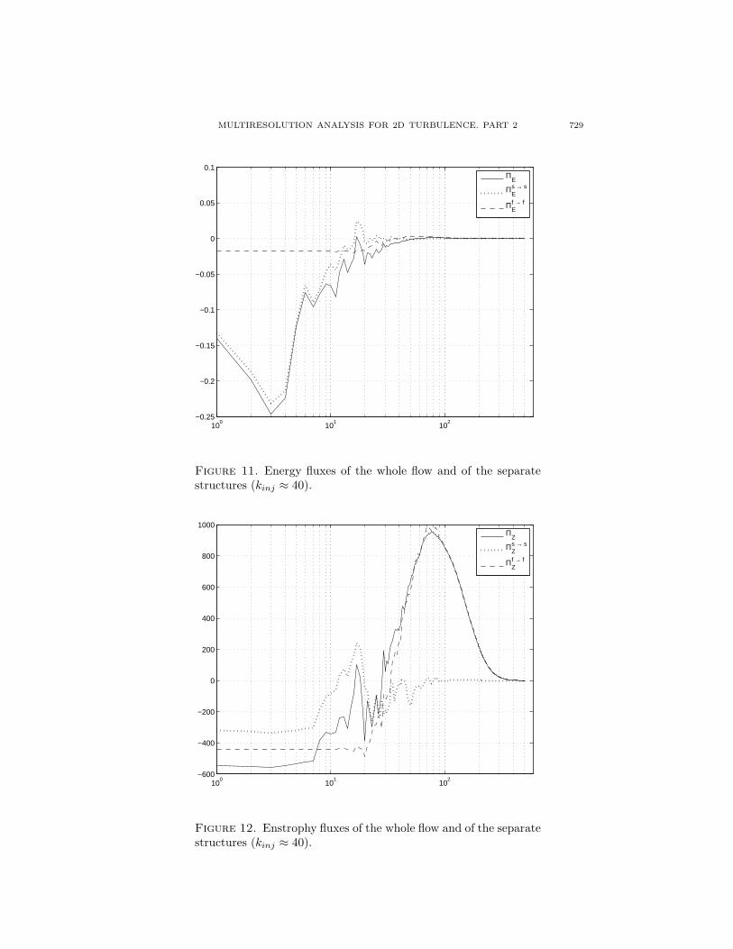
As can be expected, the inverse energy cascade has more room to take place andthe energy flux tends to go to zero at the largest scales (Figure 11) and goes backto zero close to the injection scale (k ≈ 40).The direct enstrophy cascade still exists at scales larger than the injection scale(Figure 12) and can be observed until k ≈ 100. One can also notice that the en-strophy flux crosses the zero axis around the injection scale (k ≈ 40).


100

101

102

−0.25

−0.2

−0.15

−0.1

−0.05

0

0.05

0.1

Π

E

ΠEs → s

ΠEf → f


100

101

102

−600

−400

−200

0

200

400

600

800

1000

Π

Z

ΠZs → s

ΠZf → f




4.3. The direct enstrophy cascade. In order to study the direct enstrophy cas-cade, the geometry of the numerical experiment has been modified again. Theturbulence is now created by three arrays of big cylinders.This setup produces aninjection scale kinj located around k = 9 (Re = 50000). The computations havebeen performed on a grid of size 512 × 2048. A snapshot of the vorticity fieldcorresponding to this setup is given in Figure 13.

100

101

102

−0.6

−0.5

−0.4

−0.3

−0.2

−0.1

0

0.1

ΠE

ΠEs → s

ΠEf → f


As can be verified on the corresponding energy flux given in figure 14, the injec-tion scale is too large to allow the development of a full inverse energy cascade.

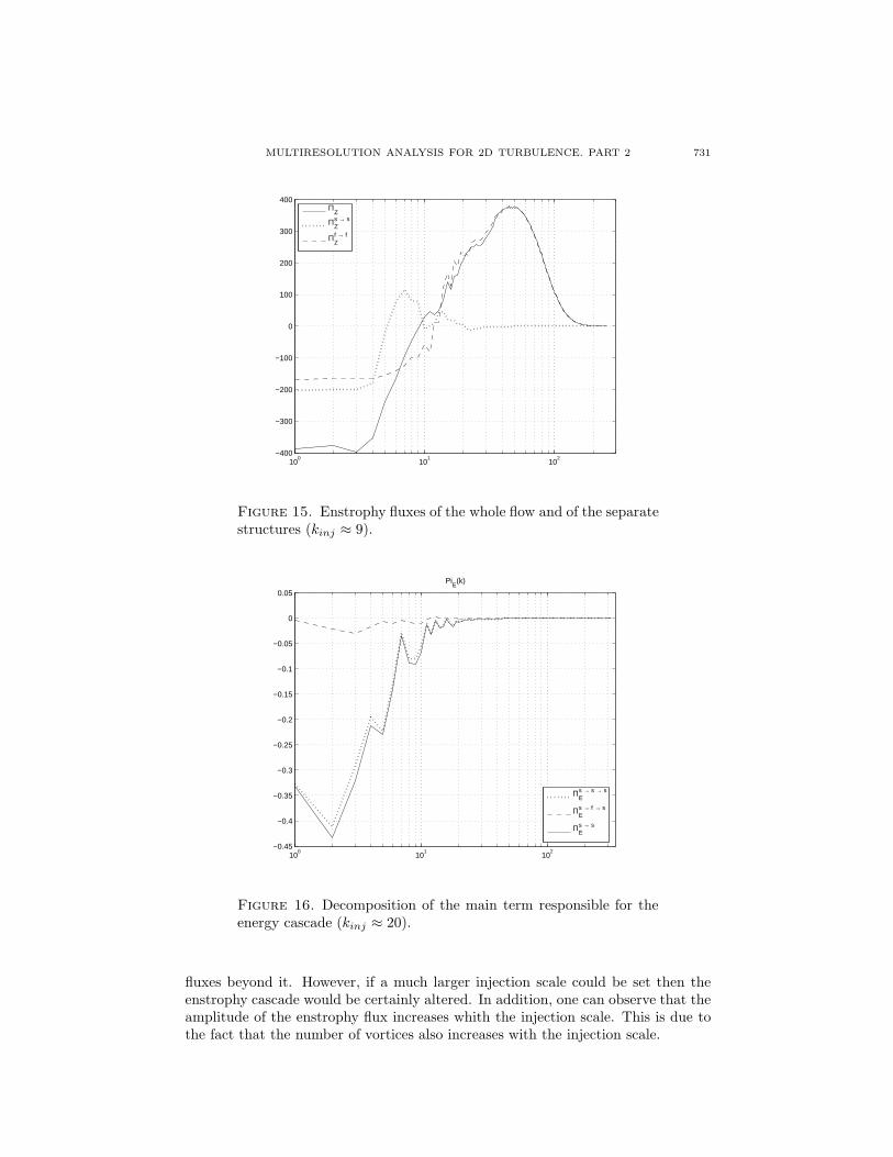
The enstrophy flux is given in Figure 15 and it can be observed on the graph thatthe direct enstrophy cascade beyond the injection scale does exist. But it can alsobe observed a strong enstrophy transfer from the injection scale toward the largestscales. One notice again that the enstrophy flux crosses the zero axis around theinjection scale (k ≈ 9).

Finally, the shifting of the injection scale from kinj ≈ 9 to k ≈ 40 essentiallyinfluences what is going on before the injection scale but modify only slightly the


100

101

102

−400

−300

−200

−100

0

100

200

300

400

Π

Z

ΠZs → s

ΠZf → f


100

101

102

−0.45

−0.4

−0.35

−0.3

−0.25

−0.2

−0.15

−0.1

−0.05

0

0.05

PiE(k)

ΠEs → s → s

ΠEs → f → s

ΠEs → s

Figure 16. Decomposition of the main term responsible for theenergy cascade (kinj ≈ 20).

fluxes beyond it. However, if a much larger injection scale could be set then theenstrophy cascade would be certainly altered. In addition, one can observe that theamplitude of the enstrophy flux increases whith the injection scale. This is due tothe fact that the number of vortices also increases with the injection scale.


100

101

102

−100

0

100

200

300

400

500

600

700

800

900

Π

Zf → f → f

ΠZf → s → f

ΠZf → f

Figure 17. Decomposition of the main term responsible for theenstrophy cascade (kinj ≈ 20).

5. Decomposition of the transport operator. We have studied in the previousparagraphs the roles played by the various structures in the global energy andenstrophy transfers and the interactions occurring between them. It is howeverpossible to specify how these interactions take place or more exactly what are themedia allowing those transfers. Indeed, thanks to the decomposition of the transportoperator itself, it will be shown in this part that the solid rotations of the vorticesare the means of transport of the energy and enstrophy transfers.

Thus the transport operator can be decomposed into two parts:

(v.∇) = (vs.∇) + (vf .∇). (23)

By performing this decomposition one can separate the energy or enstrophy trans-port due to the solid rotations from the transport due to the filaments. Finally eachterm of the equations (21) and (22) can be also split into two parts leading to thefollowing complete decompositions:

TE(k) = vs∗(k). (vs.∇)vs(k) + vs

∗(k). (vf .∇)vs(k) (24)

+ vs∗(k). (vs.∇)vf (k) + vs

∗(k). (vf .∇)vf (k)

+ vf∗(k). (vs.∇)vs(k) + vf

∗(k). (vf .∇)vs(k)

+ vf∗(k). (vs.∇)vf (k). + vf

∗(k). (vf .∇)vf (k),

and


TZ(k) = ω∗s(k). (vs.∇)ωs(k) + ω∗

s(k). (vf .∇)ωs(k) (25)

+ ω∗s(k). (vs.∇)ωf (k) + ω∗

s(k). (vf .∇)ωf (k)

+ ω∗f(k). (vs.∇)ωs(k) + ω∗

f (k). (vf .∇)ωs(k)

+ ω∗f(k). (vs.∇)ωf (k) + ω∗

f(k). (vf .∇)ωf (k).

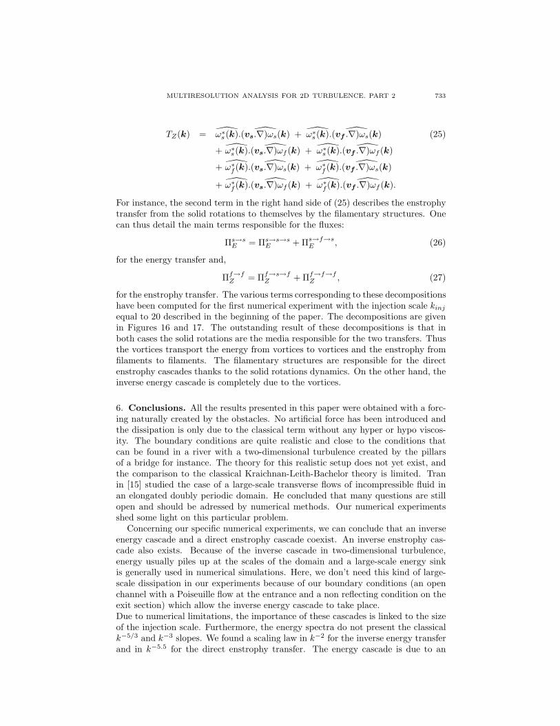
For instance, the second term in the right hand side of (25) describes the enstrophytransfer from the solid rotations to themselves by the filamentary structures. Onecan thus detail the main terms responsible for the fluxes:

Πs→sE = Πs→s→s

E + Πs→f→sE , (26)

for the energy transfer and,

Πf→fZ = Πf→s→f

Z + Πf→f→fZ , (27)

for the enstrophy transfer. The various terms corresponding to these decompositionshave been computed for the first numerical experiment with the injection scale kinj

equal to 20 described in the beginning of the paper. The decompositions are givenin Figures 16 and 17. The outstanding result of these decompositions is that inboth cases the solid rotations are the media responsible for the two transfers. Thusthe vortices transport the energy from vortices to vortices and the enstrophy fromfilaments to filaments. The filamentary structures are responsible for the directenstrophy cascades thanks to the solid rotations dynamics. On the other hand, theinverse energy cascade is completely due to the vortices.

6. Conclusions. All the results presented in this paper were obtained with a forc-ing naturally created by the obstacles. No artificial force has been introduced andthe dissipation is only due to the classical term without any hyper or hypo viscos-ity. The boundary conditions are quite realistic and close to the conditions thatcan be found in a river with a two-dimensional turbulence created by the pillarsof a bridge for instance. The theory for this realistic setup does not yet exist, andthe comparison to the classical Kraichnan-Leith-Bachelor theory is limited. Tranin [15] studied the case of a large-scale transverse flows of incompressible fluid inan elongated doubly periodic domain. He concluded that many questions are stillopen and should be adressed by numerical methods. Our numerical experimentsshed some light on this particular problem.

Concerning our specific numerical experiments, we can conclude that an inverseenergy cascade and a direct enstrophy cascade coexist. An inverse enstrophy cas-cade also exists. Because of the inverse cascade in two-dimensional turbulence,energy usually piles up at the scales of the domain and a large-scale energy sinkis generally used in numerical simulations. Here, we don’t need this kind of large-scale dissipation in our experiments because of our boundary conditions (an openchannel with a Poiseuille flow at the entrance and a non reflecting condition on theexit section) which allow the inverse energy cascade to take place.Due to numerical limitations, the importance of these cascades is linked to the sizeof the injection scale. Furthermore, the energy spectra do not present the classicalk−5/3 and k−3 slopes. We found a scaling law in k−2 for the inverse energy transferand in k−5.5 for the direct enstrophy transfer. The energy cascade is due to an


energy transfer inside the solid rotation parts of the vortices and the enstrophy cas-cade is due to an enstrophy transfer from filaments to themselves. The structuresalowing the two transfers are the solid rotation parts of the vortices.

Acknoledgement. We are very grateful to K. K. Tung for stimulating discussionsand to the referees for fruitful comments.

REFERENCES

[1] Bruneau Ch. H., Fischer P., Kellay H, The structures responsible for the two cascades in

two-dimensional turbulence, Submitted to Phys. Rev. Lett.[2] Bruneau Ch-H., Kellay H., Coexistence of two inertial ranges in two-dimensional turbulence,

Phys. Rev. E, 71 (2005), 046-305.[3] Fischer P, Multiresolution analysis for two-dimensional turbulence. Part 1: Wavelets vs Co-

sine packets, a comparative stud, Discrete and Continuous Dynamical Systems B, 5 (2005),659-686.

[4] Fischer P., Bruneau Ch.-H., Spectra and filtering: a clarification, Accepted by InternationalJournal of Wavelets, Multiresolution and Information Processing.

[5] Frisch U, “Turbulence: The legacy of A. N. Kolmogorov,” Cambridge University Press, Cam-bridge, 1995.

[6] Gkioulekas E., Tung K. K., On the Double Cascades of Energy and Enstrophy in Two Di-

mensional Turbulence. Part 1. Theoretical Formulation, Discrete and Continuous DynamicalSystems B, 5 (2005), 79-102.

[7] Gkioulekas E., Tung K. K., On the Double Cascades of Energy and Enstrophy in Two Dimen-

sional Turbulence. Part 2. Approach to the KLB Limit and Interpretation of Experimental

Evidence, Discrete and Continous Dynamical Systems B, 5 (2005), 103-124.[8] Gkioulekas E., Tung K. K., Is the subdominant part of the energy spectrum due to downscale

energy cascade hidden in quasi-geostrophic turbulence?, Discrete and Continuous DynamicalSystems B, 7 (2007), 293-314.

[9] Kellay H., Goldburg W. I., Two-dimensional turbulence: a review of some recent experiments,Rep. Prog. Phys., 65 ( 2002), 845.

[10] Kellay H., Wu X. L., Goldburg W. I., Experiments with turbulent soap films, Phys. Rev. Lett.,74 (1995), 3975.

[11] Obukhov A. M., On the distribution of energy in the spectrum of turbulent flow, Dokl. Akad.Nauk SSSR, 32 (1941), 22-24.

[12] Obukhov A. M., Spectral energy disctribution in a turbulent flow, Izv. Akad. Nauk SSSR Ser.Geogr. Geofiz., 5 (1941), 453-466.

[13] Rivera M. K., Daniel W. B., Chen S. Y., Ecke R. E., Energy and enstrophy transfer in

decaying two-dimensional turbulence, Phys. Rev. Lett., 90 (2003), 104502.[14] Rutgers M., Forced 2D turbulence: Experimental evidence of simultaneous inverse energy

and forward enstrophy cascades, Phys. Rev. Lett., 81 (1998), 2244.[15] Tran C. V., Large-scale transverse flows of incompressible fluid in an elongated doubly periodic

domain, submitted to J. Fluid Mech.[16] Tung K.K., Gkioulekas, Is the subdominant part of the energy spectrum due to downscale

energy cascade hidden in quasi-geostrophic turbulence?, Accepted by Discrete and ContinuousDynamical Systems B.

[17] Vassilicos J. C., Hunt J. C., Fractal dimensions and spectra of interfaces with application to

turbulence, Proc. R. Soc. Lond. A, 435, 505-534.

Received July 2006, revised December 2006.

E-mail address: [email protected]

MULTIRESOLUTION ANALYSIS FOR 2D TURBULENCE…pfischer/Publications_files/3.pdf · MULTIRESOLUTION...

Documents

Transcript of MULTIRESOLUTION ANALYSIS FOR 2D TURBULENCE…pfischer/Publications_files/3.pdf · MULTIRESOLUTION...