Multirate signal processing on finite fields

S.Sarkar and H.V.Poor

Abstract: The paper addresses the problem of multirate signal processing over arbitrary fields. Studies of multirate systems and filter banks have proceeded in parallel, and a wealth of results are available in literature. The authors concentrate their attention on cyclic systems. These structures are ideally suited to generalising the concepts to finite fields. The perfect reconstruction property for quadrature mirror filter banks is obtained. It is shown how the cyclic wavelet transform (CWT) can be derived from such systems; the relationships between cyclic filter banks and CWTs are explored in detail. The results obtained are potentially very well suited for speech and image encoding, as well as for fast algorithms in signal processing.

1 Introduction

In this paper, we will discuss a generalisation of the problem of multirate signal processing. A considerable body of literature is available on this subject for the discrete-time case, see for example [1-3]. Here, we will consider these ideas in the context of cyclic systems and finite fields. Cyclic systems are linear systems, whose most important property is that, in the frequency domain, the pointwise product of the discrete Fourier transform (DFT) of the system impulse response and the DFT of the input produces the DFT of the output of the system. We will further restrict our attention to only finite-length signals, and operations on them by finite impulse response (FIR) filters, i.e. the systems are considered to be characterised by FIR filters.

The study of multirate signal processing systems is closely related to the study of filter banks. Most efficient use of multirate signal processing is through the filter-bank structures [ 11. Filter banks have been widely used in digital signal processing, especially in image processing. The seminal paper on subband coding of images [4] established the connection between filter banks and image coding. Ever since then, the use of wavelets (a specific type of filter bank) for low bit-rate lossy source coding has established itself as a very popular research area. In this paper, the basics of multirate cyclic signal processing are presented. Although the results hold for any field, particular attention has been given to their structure over finite fields. Regular wavelets have been derived from subband filter structures [ 5 ] . After we formulate the basics of multirate signal processing, we will address the question of obtaining the cyclic wavelet transforms from cyclic filter banks.

It should be noted that subband coding had already established itself as a very important tool in speech processing before being applied to images [6, 71 etc.

0 IEE, 2001 ZEE Proceedings online no. 20010319 DOI: 10.1049/ip-vis:200103 19 Paper first received 6th March 2000 and in revised form 4th January 2001 S. Sarkar is with Corporate R & D, Qualcomm Incorporated, San Diego, CA 92121. USA H.V. Poor is with Princeton University, Princeton, NJ 08544, USA

254

Among other advantages, the masking effect of speech is utilised, as an error in a subband is confined only to that subband. Secondly, variation of bit-assignment among subbands can be carried out to spectrally shape the noise spectrum according to the frequency sensitivity of human hearing [8]. Needless to say, these benefits transfer in a natural way to images too, and lead to other advantages as well. These include scalable transmitting capabilities, effectiveness in extremely low bit-rate encoding, etc. One motivation for considering finite fields is to avoid rounding errors in computation and make use of the finite alphabet output of quantisers.

For a good overview of the previous literature, the reader is referred to [9, 101.

2 Background

This paper provides a common framework for linking together a variety of signal processing techniques that have been developed in the last few years. It is essential to understand a few basic concepts to appreciate the various threads that will appear in the rest of the paper. The reader is referred to the excellent references listed in the subsections for a more detailed treatment of the various subjects.

2.1 Basics of finite fields A field 3 [ 1 1, 121 is defined as a set of elements on which two binary operations, addition (+) and multiplication ( . ) are defined, so that they satisfy three conditions:

0 F is a commutative group under addition, with identity element ‘0’ with respect to addition. 0 F-{ O} is a commutative group under multiplication with identity element ‘ 1 ’ with respect to multiplication. 0 Multiplication is distributive over addition.

A finite set of q objects satisfying the axioms of a field is called a Galois field, GF(q). It can be shown that any finite field obeys the following properties:

0 GF(q) exists if and only if q = p m , where p is a prime number, and m > 1 is an integer. 0 GF(q) is unique, and any two finite fields with same number of elements are isomorphic.

IEE Pr0c:Vi.s. Image Signal Process., Vol. 148, No. 4, August 2001

0 There exists a primitive element y in GF(q) such that the q elements in GF(q) can be written as 0, 1, cp, cp2, . . . , (pqp2 . Thus, cpq-' = 1, and multiplication is cyclic over GF(q). 0 For m = 1, GF(q) is the set of integers 0, 1, 2 , . . . , p - 1, with addition and multiplication defined modulo p . 0 GF(q) is a vector space over GF(p), with basis { 1, cp, q2,. . . , y n l - ' } . Thus any x E GF(q) is uniquely written as x = ~ c i y " - ' , w h e r e O ~ c i , p , f o r i = 1 , 2 , . . . , n.This is equivalently written as a vector x = [e, , c 2 , . . . , ell].

Note that addition is simply defined as componentwise addition modulo p . Any non-zero vector is written as cp' for some 0 5 r < q - 1. r is defined as the index of x and written as ind(x). If x = y I' and y = cp s,

ind(xy) = ind(x) + ind@)(mod(q - l)), ind(x/y) = ind(x) - ind@)(mod(q - 1)).

The inverse function is called 'exp', and obeys the follow- ing laws:

exp(r) = y r , exp(ind(x)) = x, ind(exp(r)) = r .

The order s of any non-zero element x E GF(q) is defined to be the minimum strictly positive integer for which xs = 1. Thus, the element 1 has order 1, and the primitive element y has order q - 1. The primitive element can be thought of as a root of a mth degree monic polynomial P(x) which is irreducible (i.e. cannot be factorised) over GF(q). Thus, a finite field can be thought of as being generated by this polynomial. There is no straightforward way of detennin- ing this polynomial, and extensive tables for such poly- nomials exist [12]. Furthermore, there may be many polynomials that satisfy this condition, and the primitive root will vary according to the polynomial chosen. But all such generated fields will be isomorphic. Hence, one can choose any one polynomial and the corresponding primi- tive root to describe the field. The Appendix provides a table for GF(52).

2.2 Wavelets and multiresolution analysis As this paper will relate the filter banks to the cyclic wavelet structure, this Section provides a brief introduction to finite length and cyclic multiresolution analysis. Over the past decade, multiresolution analysis via wavelet decomposition has emerged as an important tool in the analysis of signals and images [ 131. Generally speaking, the principal framework within which such techniques have been studied and applied is the same as that used in the discrete-time Fourier analysis of sequences of complex numbers; that is, the sequence to be transformed is viewed as a mapping from the set of integers Z to the set of complex numbers C. Of course, Fourier analysis can also be performed on finite-length sequences of complex numbers by viewing them as mappings from a finite cyclic group to C using the DFT. The DFT and its extension to the situation in which the complex field is replaced with a finite field are of widespread use in digital signal processing applications and algebraic coding. In this Section, we briefly discuss an analogous framework for the multiresolution analysis of finite-length sequences of elements from a finite field. This framework is described in more detail in [14-161.

2.3 DFT over finite fields A useful transform over a finite field F is the number- theoretic Fourier transform. Recall that, over the complex field C, we use the nth root of unity exp(2niln) to define a

DFT of length n. To draw an analogy over the finite field, we will use any element in the field whose order is n. This can be identified as an nth root ofunity. Note that we are constrained to use this element to define the transform, as this ensures the invertibility of the transform and makes it meaningful.

Let the field in consideration be GF(pm). To define a Fourier transform of length n, there must exist at least one element of order n in the field. This is equivalent to the restriction that n Ipm - 1, where the symbol ' 1 ' stands for 'divides'. We have the following definition:

Definition 1; Let v = { v, , i = 0, I , . . . , n - 1 } be a vector over GF(p"*) where n divides (p" - 1) for some m, and let f l be an element of GF(p'?,) of order n. Then the Fourier transform of v is the vector V = { 5, j = 0, . . . , n - 1 } given by

n- I

/=O v,=c~I"v/ j = 0 , 1 , . . . , n - 1 . (1)

Here, as noted above, the element of order n can be thought of as the nth root of unity, as in the conventional DFT over the complex field. It is important to note, however, that not all lengths of DFTs are allowed over every finite field, since a length n DFT exists over CF(pm) iff nl (p" ' - l ) . The inverse transform is defined by

where n is interpreted mod q, i.e. as an integer of the field. For more details, and interesting properties of such systems, the reader is referred to [ 1 1, 17, IS]

2.4 Finite-length wavelet transforms An important class of multiresolution decompositions of (infinite-length) discrete time sequences are the so-called Laplacian pyramid schemes, in which the resolution is successively halved by recursively low-pass filtering the signal under analysis and decimating it by a factor of two. The residual (i.e. the error incurred) at each stage of this process is referred to as the 'detail' at that stage, and the sequence of details formed by this decomposition is the transform of interest. Suitable choice of the filters used in this process renders this transform invertible; and such suitable filters can be characterised through their discrete- time Fourier properties (e.g. [ 191).

The Laplacian pyramid structure can be adapted to define an exact multiresolution wavelet transform for sequences of finite length N=2", from an arbitrary field F, where n > 1 is an integer. For j= 1, 2 , . . . , n consider matrices HJ and CJ over .F of dimension 2"-J x 2"-J+I, satisfying the conditions

(HJ)*H' + (G')*GJ = N'-'Z2",+I, (3)

where I , denotes the k x k identity matrix, and where N ' c F is a constant. (Here, the asterisk denotes the adjoint.)

Within this framework, consider the following algorithm

Decomposition: Given CO = v E F2" and an integer n > 0, compute d l , . . . , dn , c" as follows:

~ 4 1 .

c ~ + I = H J + ~ ~ J dl+l = GJ+1 c . J

255 IEE Proc.-vis. lmuge Signul Process., hl. 148. No. 4, August 2001

Reconstruction: Given a decomposition {d', . . . , d", e"} , reconstruct the original signal v = co by computing, for j = n - 1 , n-2 , . . . ,0 ,

= N'[(Gi+I)*dj+' + (Hj+l)*ci+l I. The one-to-one mapping v { d ' , d 2 , . . . , d", c"] defined by decomposition/reconstruction defines a finite-length wavelet transform.

2.5 Cyclic wavelet transforms We have defined the finite-length wavelet transform in terms of the matrices GI, G 2 , . . ., G" and H ' , H 2 , . . . , H " appearing in decompositionlreconstruction. As in the case of Fourier analysis, it is of interest to constrain this transform to define a cyclic multiresolution analysis of the space of the periodic sequences of period 2" over F. This can be accomplished by constraining the matrices HJ and CJ to be 2-circulants [20] for each j, i.e. they are constrained to be of the form

where N/ gI2"-J+'. Since a 2-circulant matrix is defined completely by its first row, we can write GJ = 2-cirJgJ) and HJ = 2;cir{ hJ} where gJ and hJ denote the first rows of GJ and HJ, respectively.

Within this constraint, an interesting interpretation of the algorithm decomposition/reconstruction is possible if we consider the sequences cJ and dJ to be periodic sequences of period equal to their lengths (N,+'). In particular, for matrices satisfying eqn. 4, the ( j + 1)th step of decomposi- tion defines a finite-impulse-response (FIR) filtering of the periodic sequence e*-' with the two FIR filters having impulse response hJ and gJ, followed by a decimation by 2. The period of the input sequence cJ-' is 2"-.i+l while the period of the two output sequences CJ and dJ is 2"-J. Similarly, reconstruction can be considered to be interpola- tion by 2 followed by FIR filtering. Note that this filtering and decimation by 2 (or interpolation by 2 and filtering on the reconstruction side) is completely analogous to the subband decomposition scheme for infinite-length sequences described by the Laplacian pyramid. For a generalisation to arbitrary data lengths, see [ 151.

2.6 Finite field wavelet transforms We now consider the cyclic wavelet transform described by decomposition/reconstruction with transform matrices as in eqn. 4 for the case in which F is a finite field: F = GF(p"), where q is an odd prime and m is a positive integer. We again restrict the data length N to be a power of two, N = 2"; and we assume that N/2 divides (p" - 1). This latter condition implies the existence of an order-N/2 element a of the multiplicative sub-group of F.

Within this model, we can characterise cyclic wavelet transforms by considering the Fourier properties of g ' , g',..., g", and h' , h2 , . . . ,h" . To do so, we first define polynomials

(NP- 1

I=O ym(x) = gil+"x[, m = 0, 1

and let qm(x), m = 0, 1, be defined similarly for h' .

256

Theorem (Caire, Grossman & Poor [14]): The matrices 2-cir{g'} and 2-cir{h'} satisfy eqn. 3 f o r j = 1 if and only if, for each k = O , l , . . . , (N/2) - 1, we have

(5)

and

q"'(ak) = ( - l )"~(ak)y ' -" (a-k) , m = 0, 1 (6)

for some rational function v(x) of order N / 2 over 3 satisfying v ( ~ - ~ ) v ( a ~ ) = 1, k = O,l, . . . , (N/2) - 1.

Given two sequences g' and h' that satisfy this theorem, we want to construct a family of sequences {g ' , hJ l j = 2, . . . , n } that specifies a cyclic transform as described above. Such sequences are specified by the following result:

Corollary (141: Suppose 2-cir{g'} and 2-cir{h'} satisfy eqn. 3. For each j = 2 , . . . , n , define a length-2"-j sequences gf and h f by

&,+nl = DFT-'[{yn1(a2'-lk) I k = 0, 1, . . . ,2"-J - 111,

hJ,,,, = DFT-'[(ym(a2'-lk)lk = 0, 1, . . . ,2"-J - 1}ll

for l = O , 1,. . . ,2"-J-l , and m = 0 , 1, where the sequences y" and q'" are as above, and where the operation DFT indicates the number-theoretic discrete Fourier trans- form of appropriate length. Then GJ = 2-cir{gf} and HJ = 2-cirihJ) satisfy eqn. 3 for each j = 2, . . . , n .

In view of the theorem, we see that a procedure for specifying a finite-field cyclic wavelet transform is to choose a mother wavelet g' to satisfy eqn. 5, to choose h' according to eqn. 6, and then to choose the lower-order filters from the corollary. A large variety of such transforms can be defined, several examples of which are described in [14]. These ideas are extended to decimation of orders other than 2 in [16, 211. An example would help to clarify the principle.

Example I : Consider the field F = GF(52). As 3 124, we can define a transform of length 9 on this field. Consider the field to be generated by indexing polynomial x2 +x + 2. Then, let cp be a root of the equation that is the generator for the field. (See the Appendix for a listing of the exponents and indices for this field.) Then, the following vectors define a wavelet transform:

g , = (1, Cp, (P7 , o,o , o ,o , 0,O)

g, = @ , O , 0, 1, 9, cp', 0, 0,O) g3 = ( O , O , 0, o ,o , 0, 1, cp, Cp')

It is readily checked that (8, Ig,) = 1 + q 2 + cp I 4 = 1 for i = 1, 2, 3. The orthogonality property is evident from the structure of the vectors.

3 Decimation and interpolation

We will now develop the basic tools to analyse cyclic multirate systems. The results in this Section are funda- mentals for the analysis of any cyclic multirate system, especially for quadrature mirror filters. These ideas will be used to study filter banks, and link the concepts to the CWT developed above.

Decimators and interpolators are the basic building blocks of a multirate system. To facilitate the discussion, first the discrete Z-transform over a finite field is defined. Then, the behaviour of cyclic systems in the transform

IEE Pr0c:Vi.s. Image Signal Process., Vol. 148, No. 4, August 2001

domain is characterised. The input-output relations of the decimator and interpolator are derived, and the Section concludes with an example of a fractional rate alteration system.

3. I The discrete Z-transform We have already defined the Fourier Transform over finite fields in Section 2.3. In this section, we will define the discrete analogue of the classical Z-transform [22 ] . We will see that the DFT can be computed from the Z-transform.

Dejnition 2: Given a vector v = { v i : i = 0, . . . , n - 1 }, the polynomial

n- 1 V(z ) = V,Z' (7)

r=O

is the discrete Z-transform of the vector v.

The Fourier transform coefficients are easily evaluated from the polynomial V(z) as = V(ljl), j = 0 , 1, . . . , n - 1. We will use this polynomial extensively in the remainder of the paper.

Example 2: Consider the field GF(52). 52 - 1 = 24, and 6 124, so a length 6 DFT exists in the field. Let us consider the vector v = ( l , 1 , 0, 0 , 2 , 3). Then V(z )=l+z+ 2z4 + 3zs. The element (p4 (see the Appendix), is an element of order 6 in GF(52). Hence the Fourier transform of the vector is V = ( 2 , q8, q", 0 , q", qI6).

3.2 Linear systems In the systems under consideration, we would like to have the time domain convolution yield a result such that the Fourier coefficients can be multiplied pointwise. It is well known [23] that circular convolution uniquely achieves this purpose. Let (( . ) ) N denote modulo-N arithmetic. Then, the circular convolution of a length N sequence x[n] with a length N sequence h[n] yields a length N sequence y[n] as follows:

N - l

YbI = c x[((i)),lg[((n - m ) > N 1 i=O

This is denoted by y[n] =x[n] * g [ n ] . Then, it is easy to relate the length N discrete

Z-transforms of the two sequences too. As f i N = I in the field, we will define the following product:

Y ( z ) = X ( z ) O C(z) 4! X ( z ) C ( z ) mod(P - I )

From this, we obtain the useful relation:

~ [ n ] = ~ [ n ] * g[n] + Y(z) = X ( Z ) O G(z)

3.3 Decimation We will denote a discrete time signal from a finite field by x[ . ] . Given a vector { x [ n ] } and a positive integer M, we will define the compressed signal as:

x&] = x[nM] (8) Here M is referred to as the ratio of compression. Hence, if a signal is of length N, compression by a factor of M is possible if and only if MI N. The resultant signal will have a length NIM. We will now find the relationship between the spectrum of a signal and its compressed version.

As we have mentioned before, we require the existence of an element of order N in the field. We will assume that the field under consideration is such that this condition is

IEE Proc-Vis. Image Signal Process.. Vol. 148, No. 4, August 2001

met, i.e. N I ( p " - 1 ) . Now, as MIN, it follows that MI (p" - l), i.e. the field contains an element of order M. Specifically, if a is an element of order N, and P e N / M , then a' is an element of order M.

As d' is an Mth root of unity, then it must satisfy

M i f M I L M-I

i=O 0 otherwise (9)

To prove this, simply consider the geometric series aiL. If MIL, then each of the terms in the left-

hand side of the equation is equal to I , and hence the sum is M. Otherwise, the sum is (1 -aML) / ( l -aL). But clML = I , and aL # 1, hence the result.

Denoting w=aP, { I , 0, w2, . . . , w M - ' } form the M roots of unity in the field. Under these conditions, we can state the following result:

Lemma I : Let V(z) be the discrete Z-transform associated with the vector v. Then if vd denotes the vector v compressed by a factor M, the discrete Z-transform asso- ciated with the vector vd(z) is given by

1 M - l V,(z) = - M r=o V(u'z) .

Pro08 Let the length of vector v be N. Let us define

i f m = n M w m = { 6 otherwise

Then, from eqn. 9 1 M - l

wm = - w'mx,. M I=O

0

Example 3: Consider the field GF(52). We calculated a length 6 discrete Z-transform of the vector v = ( I , 1, 0, 0,2, 3) to be V(z) = 1 + z + 2z4 + 32'. Let us say that we want to decimate this signal by a factor of 3 . Then { I , (p8, (p I6} are the three roots of unity.

V(z ) + V(q8z) + V((p'6Z) = 3

Hence V,(z) = 1, and the decimated signal is (1, 0) as desired. Note that to evaluate the Fourier coefficients, we have to use the element cp l 2 = - 1 as the relevant root of unity in the field. Here, the Fourier transform of the decimated signal is Vd = ( I , I ) . Hence,

(v& = ( 1 + 1) /2 = I , (VJl = ( I - 1)/2 = 0.

This agrees with the result already obtained.

3.4 Interpolation Given a vector { x [ n ] } of length Nand a positive integer L, we will define the interpolated signal { x , [ n ] } of length NL as:

{ ;[n/L] if Lln xebl = otherwise

257

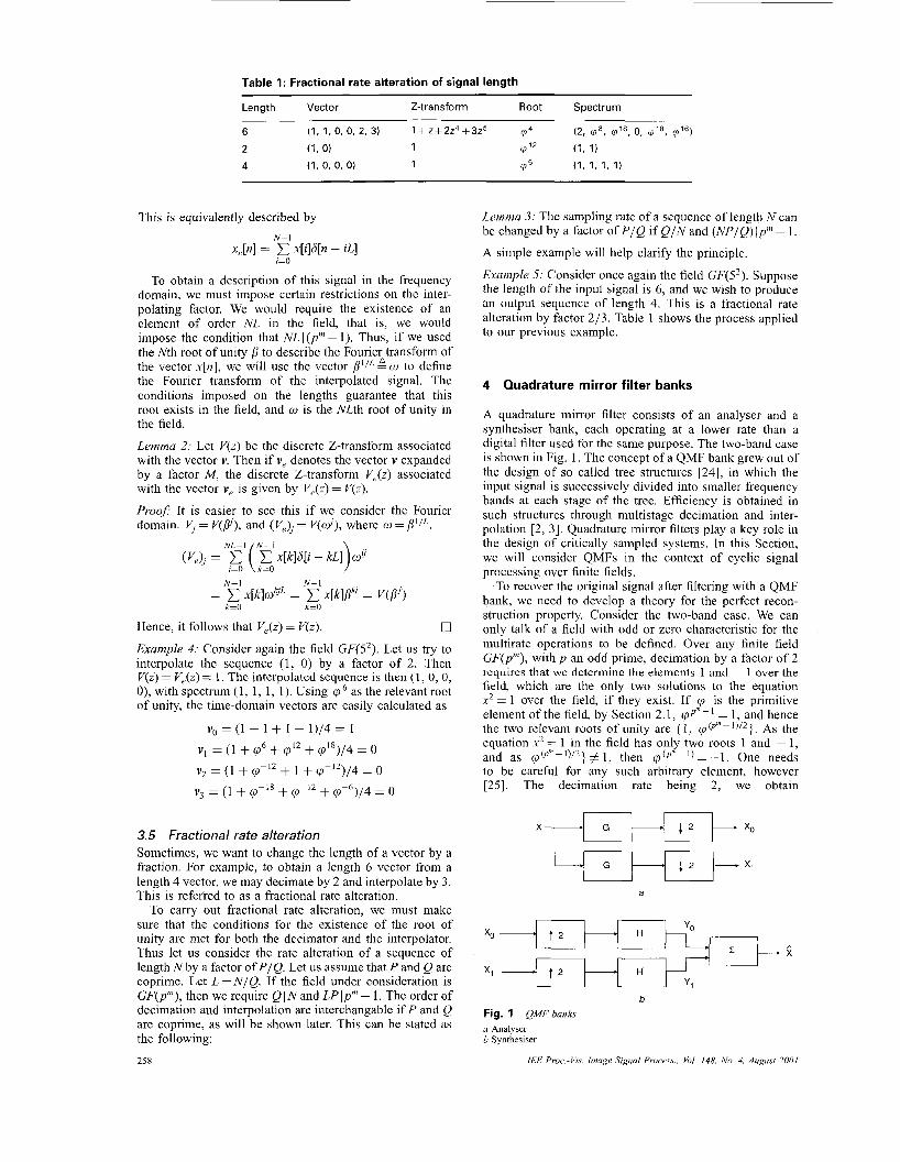
Table 1: Fractional rate alteration of signal length

Length Vector Z-transform Root Spectrum

6 (1, 1, 0, 0, 2, 3) 1 +z+2z4+3z5 cp4 (2, 478. cp18, 0. q ' 8 , q ' 6 )

2 (1. 0) 1 cp l2 (I. 1)

4 (1, 0, 0, 0) 1 q6 (1. 1, 1. 1)

This is equivalently described by N - I '. .

x,[n] = x[i]d[n - iL] i=O

To obtain a description of this signal in the frequency domain, we must impose certain restrictions on the inter- polating factor. We would require the existence of an element of order NL in the field, that is, we would impose the condition that NLI(p"- 1). Thus, if we used the Nth root of unity j to describe the Fourier transform of the vector x[n], we will use the vector 2 LC) to define the Fourier transform of the interpolated signal. The conditions imposed on the lengths guarantee that this root exists in the field, and o is the NLth root of unity in the field.

Lemma 2: Let V(z) be the discrete Z-transform associated with the vector v. Then if v, denotes the vector v expanded by a factor A4, the discrete Z-transform V J z ) associated with the vector v, is given by V,(z) = V(z). Prooj It is easier to see this if we consider the Fourier domain. vj = V(/y), and ( Ve)/ = V ( d ) , where w =

N-1 N - I

k=O k=O

Hence, it follows that V,(z) = V(z). 0 Example 4: Consider again the field CF(52). Let us try to interpolate the sequence (1, 0) by a factor of 2. Then V(z) = V,(z) = 1. The interpolated sequence is then ( 1 , 0, 0, 0), with spectrum (1, 1, 1, 1). Using cp6 as the relevant root of unity, the time-domain vectors are easily calculated as

V O = (1 + 1 + 1 + 1)/4 = 1

V I = (1 + q6 + ( p I 2 + (p'*)/4 = 0

VZ = (1 + v-12 + 1 + cp-12)/4 = 0

v, = (1 + q - ' 8 + q - ' 2 + q-6>/4 = 0

3.5 Fractional rate alteration Sometimes, we want to change the length of a vector by a fraction. For example, to obtain a length 6 vector from a length 4 vector, we may decimate by 2 and interpolate by 3. This is referred to as a fractional rate alteration.

To carry out fractional rate alteration, we must make sure that the conditions for the existence of the root of unity are met for both the decimator and the interpolator. Thus let us consider the rate alteration of a sequence of length N by a factor ofP/Q. Let us assume that P and Q are coprime. Let L = N / Q . If the field under consideration is GF(p'"), then we require Q IN and LP Ip" - 1. The order of decimation and interpolation are interchangable if P and Q are coprime, as will be shown later. This can be stated as the following:

258

Lemma 3: The sampling rate of a sequence of length N can be changed by a factor of P / Q if Q / N and (NP/Q) Ip"' - 1.

A simple example will help clarify the principle.

Example 5: Consider once again the field CF(52). Suppose the length of the input signal is 6, and we wish to produce an output sequence of length 4. This is a fractional rate alteration by factor 213. Table 1 shows the process applied to our previous example.

4 Quadrature mirror filter banks

A quadrature mirror filter consists of an analyser and a synthesiser bank, each operating at a lower rate than a digital filter used for the same purpose. The two-band case is shown in Fig. 1. The concept of a QMF bank grew out of the design of so called tree structures [24], in which the input signal is successively divided into smaller frequency bands at each stage of the tree. Efficiency is obtained in such structures through multistage decimation and inter- polation [2, 31. Quadrature mirror filters play a key role in the design of critically sampled systems. In this Section, we will consider QMFs in the context of cyclic signal processing over finite fields.

To recover the original signal after filtering with a QMF bank, we need to develop a theory for the perfect recon- struction property. Consider the two-band case. We can only talk of a field with odd or zero characteristic for the multirate operations to be defined. Over any finite field GF(pm), with p an odd prime, decimation by a factor of 2 requires that we determine the elements 1 and - 1 over the field, which are the only two solutions to the equation x2 = 1 over the field, if they exist. If cp is the primitive element of the field, by Section 2.1, qP"'-' = 1, and hence the two relevant roots of unity are { 1, ( p @ m - 1 ) / 2 >. As the equation x2 = 1 in the field has only two roots 1 and - 1, and as cp@"-')/ ' }# I , then q ( p m p l ) = - l . One needs to be careful for any such arbitrary element, however [25]. The decimation rate being 2, we obtain

b Fig. 1 QMF banks a Analyser b Synthesiser

IEE Proc.-Vis. h u g e Signal Process., Vol. 148, No. 4, August 200I

V,(z) = ;[ V(z) + V( -z)]. Hence, for the system shown in Fig. 1, we get,

X~(Z) = ;[X(Z) O G(z) +X( -Z) O G(-z)] X,(z) = $[X(Z) 0 H(z ) +X( - z ) O H ( - z ) ]

After upsampling, we get

Yo(.) = ;[X(Z) 0 G(z) + X(-z) 0 G(-z)] 0 G'(z) Y,(z) = $X(z) 0 H(z ) + X(-z) 0 H(-z)] 0 H'(z)

2 ( z ) = YO(Z) + Y,(z)

Hence, finally

= ;[X(Z) O G(z) + X(-Z) O G(-z)] 0 G'(z) + $qz) 0 H(z) + X(-z ) 0 H(-z)] 0 H'(z)

For perfect reconstruction, we require that k ( z ) =X(z). This leads to

G(-z) O G'(z) + H(-Z) H'(z) = 0 (1 1)

and G(z) O G'(z) + H(z) 0 H'(z) = 2 (12)

Note that, in general, we can allow a scaled version of the input to be the reconstructed signal. It could also be delayed. Thus, if we allow the condition

G(z) O G'(z) + H(z) O H'(z) = CZ' 0 # c E .F, 1 E Z (13)

instead of eqn. 12, we could use this condition. It should now be easy to see how to extend this to polyphase filtering. However, the existence of the proper root of unity will play a vital factor in such a decomposition, and will not be addressed here.

5 Filter banks and the cyclic wavelet transform

One of the various implementations of QMF banks uses the so-called polyphase structure. We will outline in this Section how to obtain such structures. Then, we will look at specific filter banks, and point out the relationships between the CWT and filter banks.

5.1 Interconnecting building blocks Interpolators and decimators are the basic building blocks of a multirate system. While interconnecting such building blocks, one needs to be careful, as the output of the filters will not necessarily be the same. Consider the following example:

Example 6: Let us consider the sequence (1, 2, 1, 2) through a cyclic system, in a field properly chosen. Let us decimate by two and interpolate by four, and compare the two results.

v = (1,2, 1,2) (14)

(15) Vd = (1, 1)

vde = (1, 0, 0, 0, 1, 0, 0, 0)

v, = (1, o ,o , 0 , 2 , 0 , 0 , 0 , 1, o,o, 0 ,2 , o ,o , 0)

On the other hand

V,d = (1 ,0 ,2 ,0 , 1 , 0 , 2 , 0 ) (16)

Clearly, from eqns. 15 and 16, we obtain different results by simply interchanging the order of the two building blocks. In fact we can state the following:

IEE Proc -VIS Image Signal Process, Vol 148, No 4, AuguAt 2001

Lemma 4: Interpolating by L followed by decimating by M is equivalent to decimating by L followed by interpolating by L if and only if L and M are coprime.

ProoJ The proof follows from noting the fact that the set { 1, b, b2,. . . , OM- ' ] is same as the set { 1, P L , f 1 2 L , . . . ,

U In general, provided the relevant root of unity exists, an FIR filter and a decimator/interpolator can be inter- changed. The equivalent of this result for discrete time systems is captured by the so-called Noble identities [26].

pL@'- ' ) } if and only if L and A4 are coprime.

5.2 Polyphase representation To explain the basic idea of polyphase representation, it will be easier to consider an example: Let us consider a length N filter H(z) = C;"=;r' hizi, where N is even. Then, we can write

n=O n=O

Setting

i=O

and

i=O

the following can be written:

H(z ) = E&) + ZE, (2) (17)

This is a so-called polyphase decomposition of the filter H. The idea is easily extended further to obtain the following two kinds of polyphase decomposition:

Gpe Zpolyphase: Given a filter of length Nand an integer M such that MIN, the decomposition

M- 1 H(z ) = Ei(P)z '

1=0

where

n=O

is called a polyphase decomposition of type I.

Type Ilpolyphase: Given a filter of length N and an integer M such that MI N, the decomposition

M-1 H(z ) = R;(P)P- - l - f

1 4

where

R,(z) = EM-l-i(z), i = 0, 1, . . . , M - 1

is called a polyphase decomposition of type 11. Polyphase representations allow for more efficient

implementation of these filters. Such structures have been known to reduce the number of multiplications required in many signal processing applications [ 5 , 261. It is also interesting to note that the polyphase representation is also the easiest way of designing filter banks [26]. In the polyphase domain, it can be shown that the design of the QMF banks in many cases reduces to the problem of factorisation of certain matrices over a finite field [5]. The cyclic filter banks are no exception to this, and can

259

be treated in a similar way. Here is a simple example to clarify the principle.

Example 7: The earliest known QMF banks were of the following form:

H(z) = G(-Z) (18) G’(z) = G(z) H’(z) = -H(z) (19)

It is easy to see that they satisfy the conditions for an alias- free system. All the filters are derived from the single filter. The base filter G(z) is typically chosen to be low-pass, so that transformation by eqn. 18 makes GI a high-pass filter. Of course, care must be taken to make sure that the perfect reconstruction property is met, implying that the FIR filter is a sum of two delays [5].

5.3 Cyclic wavelet transform and filter banks The CWT looks at filters with transfer functions of the following form:

G‘ = G* (20) H I = H* (21)

where e. denotes the adjoint of the operator Q. If the filter G is represented in the transform domain by G(z), then the adjoint can be represented by the filter G(l/z). The CWT conditions can be rewritten in this form as

G(z) 0 G( 1 /z) = H(z) O H( 1 /z) = 1

and G(z) 0 H( 1 / z ) = 0

This is equivalent to

G( 1 / z ) 0 H(z) = 0

Clearly then

G(z) 0 G( 1 / z ) + H(z ) 0 H( 1 / z ) = 2

satisfying eqn. 12. Also observe that eqn. 11 gives us

G(-Z) O G*(z) + H(-Z) O H*(z) = 0

G( -2) O G( 1 / z ) O H(z) O G(z) +H(-z) 0 H( 1 /z) 0 G(z) 0 H(z) = 0

by the commutativity of the operation 0. This is obviously satisfied for this class of filters, and hence the CWTs are a special class of cyclic QMF filters.

Example 8: Consider only two subbands. Let the field under consideration be GF(5), and N’=3( =;) (see Section 2.6). A routine calculation gives us a length 4 transform as

g’ = (1 ,4 ,0 ,0 )

g2 = (194)

h’ = (4,4, 0,O)

h2 = (4,4)

Note that 4 = - l(mod 5), so the number 4 can be viewed as - 1 over GF(5). This gives the filters their high-pass and low-pass characteristics. Each level of transform can denote an independent filter pair.

6 Construction of filter banks

In the previous Sections, we have demonstrated how to construct filter banks from a mother wavelet, and we have shown necessary and sufficient conditions for a sequence to be a mother wavelet. Now we will explore these

260

conditions to establish some explicit equations from which mother wavelets, and thus polyphase filter banks, can be constructed.

Let us first consider the case when the mother wavelet is real. This is of great practical interest in building multilevel-error protection codes [27]. It is trivially true that a wavelet of the form (a , 0, . . . , 0) exists, where a is an element of the field of interest, as long as a # 0. We need a2 = l /N’ . We first consider the possibility of a wavelet with exactly three consecutive nonzero coefficients.

Let us first consider the case when only the first four coefficients are allowed to be nonzero. Then, for k=O, 1 , . . . , (N /2 ) - 1,

Then,

= go’ + g: + 2go g2 cosr;)

Similarly

Thus, for the theorem in Section 2.6 to hold, we must have,

Clearly, in this construction, a mother wavelet consisting of exactly three consecutive nonzero elements is not allowed in this formulation [ 141.

For the first 2R ( s n ) nonzero coefficients, by similar arguments, we must have for k = 0, 1, . . . , R - 2

,2k( I=k+l g21) + g 2 k + l ( I=k+l g21+1) = O

(23)

Example 9: As an example, consider a wavelet with its first six coefficients nonzero. Then, by eqn. 22, the relations are

gokz + gJ = gi(g3 + g5)

g2 g4 = g3 g5

Then (0, -1.5, 2, -1, -0.5, 1, 0,. . . ,0) is a possible wavelet that also satisfies the band-pass condition.

JEE Proc.-Vis. Image Signal Process., Vol. 148, No. 4, August 2001

In general, over the complex field, the conditions are, for k=O, 1, . . . , R-2

R- 1

I=k+ I (24)

2 1 2R- I

I=O

For the finite-field case, we come up with exactly the same set of conditions as for the real case: we must have for k=O, 1, . . . , R-2

g 2 k ( i=k+l 821) +g2k+l ( l=k+l 8 2 1 1 1 ) =

1 2R- 1

k 0

Example IO: Now consider a wavelet with its first six coefficients nonzero. Let the wavelet have length 8 and the field be GF(5). Then, 23-’ l (5- 1) and the primitive element q =2. Then, by eqn. 25, the relations are

gOk2 + g4) = g l k 3 + g5)

g2 g4 = g3 g5

5 1 c g : =N’ I=O

Then (0, 1, 2, 4, 2, 1, 0 , . . . , 0 ) is a possible wavelet that also satisfies the band-pass condition. Here N’ = 1 .

We have thus shown how to form filter banks explicitly by using mother wavelets. An important advantage of the cyclic wavelet analysis over cyclic Fourier analysis is lower computational complexity. If the rows of the matrices GI and HJ each have at most Mnonzero elements, then the full decomposition requires at most 2(2M- l ) ( N - 1) - O(N) operations. By comparison, the FFT has O(N log,(N)) complexity. Thus, if wavelet transforms can be used to perform tasks that are normally performed using FFTs, some practical advantage may be gained. However, like their discrete-time counterparts, these transforms may be fundamentally better suited to some tasks than are Fourier transforms.

Potential applications areas for finite-field filter banks are similar to those for the cyclic Fourier transform, or for the discrete wavelet transform. For example, the multi- resolution properties of the finite-field wavelet transform can be exploited to develop useful families of error- correcting codes featuring multilevel error protection [27]. Alternatively, the multiscale/multilocation aspects of the cyclic wavelet transform make them useful in searching for structure in long strings of elements from a finite field [28].

7 Conclusion

In this paper, we have discussed the main issues pertaining to a multirate cyclic signal processing system. The results obtained are well suited for generalisation to finite fields. Speech analysis, image processing, bandwidth compres- sion, radar/sonar processing, and spectral parameterisation of signals are some of the areas in which this concept arises naturally, and has found widespread application. The implementation and design of such cyclic filter banks are a subject of future research. It is, however, intuitively

IEE Proc.-Vis. Image Signal Process., Vol. 148, No. 4, August 200J

pleasing to note that the cyclic wavelet transform can be derived from the cyclic filter banks, as has been the case for classical filter banks and wavelets.

8 Acknowledgment

This research was supported in part by the US Office of Naval Research under Grant # NO00 14-00- 1-0 14 1.

9

1

2

3

4

5

6

7

8

9

References

VETTERLI, M., and HERLEY, C.: ‘Wavelets and filter banks: theory and design’, IEEE Trans. Signal Process., July 1992,40, pp. 2207-2232 CROCHIERE, R.E., and RABINER, L.R.: ‘Multirate digital signal processing’ (Prentice Hall, Englewood Cliffs, NJ, 1983) LIM, J.S., and OPPENHEIM, A.V. (Eds.): ‘Advanced topics in signal processing’ (Prentice Hall, Englewood Cliffs, NJ, 1988) WOODS, J.W., and O’NEIL, S.D.: ‘Subband coding of images’, IEEE Trans. Acoust. Speech Signal Process., Oct. 1986, ASSP-34, pp. 1278- 1288 VETTERLI, M., and KOVACEVIC, J.: ‘Wavelets and subband coding’ (Prentice-Hall, Englewood Cliffs, NJ, 1995) JAYANT, N.: ‘Signal compression: technology targets and research directions’, IEEE 1 Sel. Areas Commun., June 1992, 10, pp. 796-818 JOHNSTON, J.D.: ‘Transform coding of audio signals using perceptual noise criteria’, IEEEJ Se/. Areas Commun., 1988, 6 , pp. 314-323 JAYANT, N., and NOLL, P.: ‘Digital coding of waveforms’ (Prentice Hall, Englewood Cliffs, NJ, 1984) VAIDYANATHAN, PE: ‘Quadrature mirror filter banks, M-band exten- sions and perfect-reconstruction techniques’, Proc. IEEE, July 1987, 4, nn 4-31

10 YAIDYANATHAN, P.P.: ‘Multirate digital filters, filter banks, polyphase networks, and applications: A tutorial’, Proc. IEEE, Jan. 1990, 78, (l), pp. 65-93

1 1 BLAHUT, R.E.: ‘Theory and practice of error control codes’ (Springer- Verlag, New York, NY, 1983)

12 LIDL, R., and NIEDERREITER, H.: ‘Introduction to finite fields and its applications’ (Cambridge University Press, Reading, MA, 1986)

13 DAUBECHIES, 1.: ‘The wavelet transform, time-frequency localization and signal analysis’, IEEE Trans. In$ Theory, Sept. 1990, 36, pp. 961- 1005

14 CAIRE, G., GROSSMAN, R.L., and POOR, H.V.: ‘Wavelet transforms associated with finite cyclic groups’, IEEE Trans. In$ Theory, July 1993, 37, (S), pp. 1157-1 166

15 SARKAR, S.: ‘Cyclic wavelet transforms and error control coding’ PhD thesis, Princeton University, Aug. 1996

16 SARKAR, S., and POOR, H.V: ‘Cyclic wavelet transforms for arbitrary finite data lengths’, SignalProcess., Dec. 2000,80, (12), pp. 2541-2552

17 BLAHUT, R.E.: ‘Fast algorithms for digital signal processing’ (Addison-Wesley, 1985)

18 BLAHUT, R.E.: ‘Algebraic methods for signal processing and commu- nications coding’ (Springer-Verlag, New York, NY, 1992)

19 MALLAT, S.G.: ‘A theory of multiresolution signal decomposition: The wavelet representation’, IEEE Truns. Pattern Anal. Mach. Intell., 1989 11, pp. 674-693

20 DAVIS, P.J.: ‘Circulant matrices’ (Wiley, New York, NY, 1979) 21 SARKAR, S., and POOR, H.V.: ‘Certain generalizations of the cyclic

22

23

24

25 26

27

28

wavelet transform’. Proceedings of Conf. Iiform. Sci. Syst., The johns Hopkins University, 22-24 Mar. 1995 OPPENHEIM, A V , WILSKY, A S . , and YOUNG, I.T.: ‘Signals and systems’ (Prentice Hall, Englewood Cliffs, NJ, 1983) OPPENHEIM, AV., and SCHAFER, R.W.: ‘Discrete time signal processing’ (Prentice Hall, Englewood Cliffs, NJ, 1989) DUDGEON, D.E., and MERSEREAU, R.W. (Eds.): ‘Multidimensional signal processing’ (Prentice Hall, Englewood Cliffs, NJ, 1984) HERSTEIN, I.N.: ‘Topics in algebra’ (Macmillan, New York, NY, 1990) VAIDYANATHAN, PP.: ‘Multirate systems and filter banks’ (Prentice Hall, Englewood Cliffs, NJ, 1993) SARKAR, S., and POOR, H.V.: ‘Finite-field wavelet transforms and multilevel error protections’. Proceedings of 1995 IEEE Int’l Symp. Inform. Theory, Whistler, BC, 17-22 Sept. 1995 BENSON, D.C.: ‘Digital signal processing methods for biosequence analysis’, Nucleic Acids Res., 1990, 18, (lo), pp. 3001-3006

10 Appendix

Table 2 is the listing of the field GF(52)/x2 +x + 2 with primitive element q . Note that the exponent 00 corre- sponds to the element 0, which is not a part of the multiplicative subgroup of the field and hence is omitted. Multiplication by 0 will yield 0 as the result, and division by 0 is not permitted.

26 1

Table 2: GF(5*)

Exponent Index Exponent Index Exponent Index

01 0

10 1

43 2

42 3

32 4

44 5

02 6 20 7

31

34

14

33

04

40

12

13

8 23

9 11

10 03

11 30

12 24

13 21

14 41

15 22

16 17

18 19

20

21 22

23

Exponent n refers to the element cp" in the field. To add any two elements, do modulo 5 addition on each of the co- ordinates of the exponent, and look up the resultant from the Table. For example,

1 * 1 + cp * cp + cp7 * cp7 = 1 + cp2 + cp14

= (01) + (43) + (12) = (01) = cpo = 1

262 IEE Proc.-Vis. Image Signal Process., Vol. 148, No. 4, August 2001