Multiplication and Composition Operators on Weak L · PDF fileMultiplication and Composition...

Multiplication and Composition Operators onWeak Lp spaces

Rene Erlin Castillo1, Fabio Andres Vallejo Narvaez2

and Julio C. Ramos Fernandez3

Abstract

In a self-contained presentation, we discuss the Weak Lp spaces.Invertible and compact multiplication operators on WeakLp are char-acterized. Boundedness of the composition operator on Weak Lp isalso characterized.Keywords: Compact operator, multiplication and composition oper-ator, distribution function, Weak Lp spaces.

Contents

1 Introduction 2

2 Weak Lp spaces 2

3 Convergence in measure 7

4 An interpolation result 13

5 Normability of Weak Lp for p > 1 25

6 Multiplication Operators 39

7 Composition Operator 49

A Appendix 52

02010 Mathematics subjects classification primary 47B33, 47B38; secondary 46E30

1

1 Introduction

One of the real attraction of WeakLp space is that the subject is sufficientlyconcrete and yet the spaces have fine structure of importance for applications.WeakLp spaces are function spaces which are closely related to Lp spaces. Wedo not know the exact origin of Weak Lp spaces, which is a apparently partof the folklore. The Book by Colin Benett and Robert Sharpley[4] containsa good presentation of WeakLp but from the point of view of rearrangementfunction. In the present paper we study the WeakLp space from the point ofview of distribution function. This circumstance motivated us to undertakea preparation of the present paper containing a detailed exposition of thesefunction spaces. In section 6 of the present paper we first prove a charac-terization of the boundedness of Mu in terms of u, and show that the setof multiplication operators on Weak Lp is a maximal abelian subalgebra ofB(WeakLp

), the Banach algebra of all bounded linear operators on WeakLp.

For the systemic study of the multiplication operator on different spaces werefereed to ([1], [2], [5] [3], [10], [18], [21]).We use it to characterize the invertibility of Mu on Weak Lp. The compactmultiplication operators are also characterized in this section.In section 7 a necessary and sufficient condition for the boundedness of com-position operator CT is given. For the study of composition operator ondifferent function spaces we refereed to ([6], [11], [12], [16], [18], [19]).

2 Weak Lp spaces

Definition 2.1. For f a measurable function on X, the distribution functionof f is the function Df defined on [0,∞) as follows:

Df (λ) := µ({x ∈ X : |f(x)| > λ}

). (1)

The distribution function Df provides information about the size of f butnot about the behavior of f itself near any given point. For instance, a func-tion on Rn and each of its translates have the same distribution function. Itfollows from definition 2.1 that Df is a decreasing function of λ (not neces-sarily strictly).

Let (X,µ) be a measurable space and f and g be a measurable functions on(X,µ) then Df enjoy the following properties: For all λ1, λ2 > 0:

2

1. |g| ≤ |f | µ-a.e. implies that Dg ≤ Df ;

2. Dcf (λ1) = Df

(λ1|c|

)for all c ∈ C/{0};

3. Df+g(λ1 + λ2) ≤ Df (λ1) +Dg(λ2);

4. Dfg(λ1λ2) ≤ Df (λ1) +Dg(λ2).

For more details on distribution function see ([7] and [15]).Next, Let (X,µ) be a measurable space, for 0 λ}) ≤

(C

λ

)p},

for some C > 0. Observe that Weak L∞ = L∞.

Weak Lp as a space of functions is denoted by L(p,∞).

Proposition 2.1. Let f ∈Weak Lp with 0 0 : Df (λ) ≤

(C

λ

)p}=

(supλ>0

λpDf (λ)

)1/p

= supλ>0

λ {Df (λ)}1/p .

Proof. Let us define

λ = inf

{C > 0 : Df (α) ≤

(C

α

)p},

and

B =

(supα>0

αpDf (α)

)1/p

.

Since f ∈Weak Lp, then

Df (α) ≤(C

α

)p,

for some C > 0, then

3

{C > 0 : Df (α) ≤

(C

α

)p∀ α > 0

}6= ∅.

On the other handαpDf (α) ≤ Bp,

thus {αpDf (α) : α > 0} is bounded above by Bp and so B ∈ R.Therefore

λ = inf

{C > 0 : Df (α) ≤

(C

α

)pα > 0

}≤ B. (2)

Now, let ε > 0, then there exists C such that

λ ≤ C < λ+ ε,

and thus

Df (λ) ≤ Cp

λp<

(λ+ ε)p

λp,

then

supλ>0

λpDf (λ) < (λ+ ε)p(supλ>0

λpDf (λ)

)1/p

≤ λ

B < λ, (3)

by (2) and (3) B = λ.

Definition 2.2. For 0 0 : Df (λ) ≤

(C

λ

)p∀λ > 0

}=

(supλ>0

λpDf (λ)

)1/p

= supλ>0

λ {Df (λ)}1/p ,

is finite. Two functions in L(p,∞) will be considered equal if they are equalµ−a.e.

4

The Weak Lp = L(p,∞) are larger than the Lp spaces, we have the following.

Proposition 2.2. For any 0 λ}

)≤

∫{|f |>λ}

|f |p du ≤∫X

|f |p du =∥∥f∥∥p

Lp,

therefore

µ({x ∈ X : |f(x)| > λ}

)≤(‖f‖Lpλ

)p. (4)

Hence f ∈ Weak Lp = L(p,∞), which means that

Lp ⊂ L(p,∞). (5)

Next, from (4) we have(supλ>0{λpDf (λ)}

)1/p

≤∥∥f∥∥

Lp∥∥f∥∥L(p,∞)

≤∥∥f∥∥

Lp.

Remark 2.1. The inclusion (5) is strict, indeed, let f(x) = x−1/p on (0,∞)(with the Lebesgue measure). Note

m

({x ∈ (0,∞) :

1

|x|1/p> λ

})= m

({x ∈ (0,∞) : |x| < 1

λp

})= 2λ−p.

Thus f ∈Weak Lp(0,∞), but∫ ∞0

(1

x1/p

)pdx =

∫ ∞0

dx

x→∞,

then f /∈ Lp(0,∞).

5

Proposition 2.3. Let f, g ∈ L(p,∞). Then

1.∥∥cf∥∥

L(p,∞)= |c|

∥∥f∥∥L(p,∞)

for any constant c,

2.∥∥f + g

∥∥L(p,∞)

≤ 2(∥∥f∥∥p

L(p,∞)+∥∥g∥∥p

L(p,∞)

)1/p.

Proof. (1) For c > 0 we have

µ({x ∈ X : |cf(x)| > λ}

)= µ

({x ∈ X : |f(x)| > λ

c

}),

thus

Dcf (λ) = Df

(λ

c

).

And thus

‖cf‖L(p,∞)=

(supλ>0

λpDcf (λ)

)1/p

=

(supλ>0

λpDf

(λ

c

))1/p

=

(supcw>0

cpwpDf (w)

)1/p

= c

(supcw>0

wpDf (w)

)1/p

,

then‖cf‖L(p,∞)

= c‖f‖L(p,∞).

(2) Note that{x ∈ X : |f(x)+g(x)| > λ

}⊆{x ∈ X : |f(x)| > λ

2

}⋃{x ∈ X : |g(x)| > λ

2

}.

Hence

µ({x ∈ X : |f(x) + g(x)| > λ}

)≤ µ

({x ∈ X : |f(x)| > λ

2

})+ µ

({x ∈ X : |g(x)| > λ

2

}),

then

λpDf+g(λ) ≤λpDf

(λ

2

)+ λpDg

(λ

2

)λpDf+g(λ) ≤2p

[supλ>0

λpDf (λ) + supλ>0

λpDg(λ)

],

6

therefore (supλ>0

λpDf+g(λ)

)1/p

≤2(∥∥f∥∥p

L(p,∞)+∥∥g∥∥p

L(p,∞)

)1/p∥∥f + g

∥∥L(p,∞)

≤2(∥∥f∥∥p

L(p,∞)+∥∥g∥∥p

L(p,∞)

)1/p.

Remark 2.2. Proposition 2.3 (2) tell us that ‖.‖L(p,∞)define a quasi-norm

on L(p,∞).

Definition 2.3. A quasi-norm is a functional that is like a norm except thatit does only satisfy the triangle inequality with a constant C ≥ 1, that is

‖f + g‖ ≤ C(‖f‖+ ‖g‖

).

3 Convergence in measure

Next, we discus some convergence notions. The following notion is of impor-tance in probability theory.

Definition 3.1. Let f, fn (n = 1, 2, 3, ...) be a measurable functions on themeasurable space (X,µ). The sequence {fn}n∈N is said to converge in measure

to f (fnµ→ f) if for all ε > 0 there exists an n0 ∈ N such that

µ({x ∈ X : |fn(x)− f(x)| > ε}

)< ε for all n ≥ n0. (6)

Remark 3.1. The preceding definition is equivalent to the following state-ment.For all ε > 0,

limn→∞

µ({x ∈ X : |fn(x)− f(x)| > ε}

)= 0. (7)

Cleary (7) implies (6). To see the convergence given ε > 0, pick 0 < δ < εand apply (6) for this δ.There exists an n0 ∈ N such that

µ({x ∈ X : |fn(x)− f(x)| > δ}

)< δ,

7

holds for n ≥ n0. Since

µ({x ∈ X : |fn(x)− f(x)| > ε}

)≤ µ

({x ∈ X : |fn(x)− f(x)| > δ}

).

We concluded that

µ({x ∈ X : |fn(x)− f(x)| > ε}

)< δ,

for all n ≥ n0. Let n→∞ to deduce that

lim supn→∞

µ({x ∈ X : |fn(x)− f(x)| > ε}

)≤ δ. (8)

Since (8) holds for all 0 < δ < ε (7) follows by letting δ → 0.

Remark 3.2. Convergence in measure is a more general property than con-vergence in either Lp or L(p,∞), 0 < p < ∞, as the following propositionindicates:

Proposition 3.1. Let 0 0 we have:

µ({x ∈ X : |fn(x)− f(x)| > ε}

)≤ 1

εp

∫X

|fn − f |p dµ

εpµ({x ∈ X : |fn(x)− f(x)| > ε}

)≤ ‖fn − f‖pLp

supλ>0

λpDfn−f (λ) ≤ ‖fn − f‖pLp ,

and thus‖fn − f‖L(p,∞)

≤ ‖fn − f‖Lp .

This shows that convergence in Lp implies convergence in WeakLp. The casep =∞ is tautological.

(2) Give ε > 0 find an n0 ∈ N such that for n > n0, we have

8

‖fn − f‖L(p,∞)=

(supλ>0

λpDfn−f (λ)

)1/p

< ε1p+1,

then taking λ = ε, we conclude that

εpµ({x ∈ X : |fn(x)− f(x)| > ε}

)< εp+1,

for n > n0.Hence

µ({x ∈ X : |fn(x)− f(x)| > ε}

)< ε for n > n0.

Example 3.1. Fix 0 0}

)=

1

k,

thuslimk→∞

m({x ∈ [0, 1] : fk,j(x) > 0}

)= 0,

that is fk,jm−→ 0.

Likewise, Observe that

‖fk,j‖L(p,∞)=

(supλ>0

λpm({x ∈ [0, 1] : fk,j(x) > λ}

))1/p

≥(

supk≥1

k − 1

k

)1/p

= 1.

Which implies that fk,j does not converge to 0 in L(p,∞).

It turns out that every sequence convergent in L(p,∞) has a subsequence thatconverges µ-a.e. to the same limit.

Theorem 3.1. Let fn and f be a complex-valued measurable functions on ameasure space (X,A, µ) and suppose fn

µ−→ f . Then some subsequence offn converges to f µ−a.e.

9

Proof. For all k = 1, 2, ... choose inductively nk such that

µ({x ∈ X : |fn(x)− f(x)| > 2−k}

)< 2−k, (9)

and such that n1 < n2 < ... < nk < ... Define the sets

Ak ={x ∈ X : |fnk(x)− f(x)| > 2−k

},

(9) implies that

µ

(∞⋃k=m

Ak

)≤

∞∑k=m

µ(Ak) ≤∞∑k=m

2−k = 21−m, (10)

for all m = 1, 2, 3, ... It follows from (10) that

µ

(∞⋃k=1

Ak

)≤ 1 <∞. (11)

Using (10) and (11), we conclude that the sequence of the measure of the

sets

{∞⋃k=m

Ak

}m∈N

converges as m→∞ to

µ

(∞⋂m=1

∞⋃k=m

Ak

)= 0. (12)

To finish the proof, observe that the null set in (12) contains the set of allx ∈ X for which fnk(x) does not converge to f(x).

Remark 3.3. In many situations we are given a sequence of functions andwe would like to extract a convergent subsequence. One way to achieve thisis via the next theorem which is a useful variant of theorem 3.1. We firstgive a relevant definition.

Definition 3.2. We say that a sequence of measurable functions {fn}n∈N onthe measure space (X,A, µ) is Cauchy in measure if for every ε > 0 thereexists an n0 ∈ N such that for n, m > n0 we have

µ({x ∈ X : |fn(x)− fm(x)| > ε}

)< ε.

10

Theorem 3.2. Let (X,A, µ) be a measure space and let {fn}n∈N be a complexvalued sequence on X, that is Cauchy in measure. Then some subsequenceof fn converges µ−a.e.

Proof. The proof is very similar to that of theorem 3.1 for all k = 1, 2, 3, ...choose nk inductively such that

µ({x ∈ X : |fnk(x)− fnk+1

(x)| > 2−k})< 2−k, (13)

and such that n1 < n2 < n3 < ... < nk < nk+1 < ... Define

Ak ={x ∈ X : |fnk(x)− fnk+1

(x)| > 2−k}.

As shown in the proof of theorem 3.1 (13) implies that

µ

(∞⋂m=1

∞⋃k=m

Ak

)= 0, (14)

for x /∈∞⋃k=m

Ak and i ≥ j ≥ j0 ≥ m (and j0 large enough) we have

|fni(x)− fnj(x)| ≤i−1∑l=j

|fnl(x)− fnl+1(x)| ≤

i∑l=j

2−l ≤ 21−j ≤ 21−j0 .

This implies that the sequence {fni(x)}i∈N is Cauchy for every x in the set(∞⋃k=m

Ak

)cand therefore converges for all such x. We define a function

f(x) =

limj→∞

fnj(x) when x /∈∞⋂m=1

∞⋃k=m

Ak

0 when x ∈∞⋂m=1

∞⋃k=m

Ak

Then fnj → f almost everywhere.

Proposition 3.2. If f ∈ Weak Lp and µ({x ∈ X : f(x) 6= 0}

)< ∞, then

f ∈ Lq for all q < p. On the other hand, if f ∈ Weak Lp ∩ L∞ then f ∈ Lqfor all q > p.

11

Proof. If p <∞, we write∫X

|f(x)|q dµ = q

∞∫0

λq−1Df (λ) dλ

= q

1∫0

λq−1Df (λ) dλ+ q

∞∫1

λq−1Df (λ) dλ.

Note that

µ({x ∈ X : |f(x)| > λ}

)≤ µ

({x ∈ X : f(x) 6= 0}

).

Therefore µ({x ∈ X : |f(x)| > λ}

)≤ C, then

∫X

|f(x)|q dµ ≤ qC

1∫0

λq−1 dλ+ qC

∞∫1

λq−p−1 dλ = C +qCλq−p

q − p

]∞1<∞

Therefore f ∈ Lq.

If f ∈Weak Lp ∩ L∞. Then

∫X

|f(x)|q dµ = q

∞∫0

λq−1Df (λ) dλ

= q

M∫0

λq−1Df (λ) dλ+ q

∞∫M

λq−1Df (λ) dλ,

where M = esssup|f(x)|. Note that

µ({x ∈ X : |f(x)| > λ}

)= 0 for λ > M,

since f ∈Weak Lp ∩ L∞, therefore

q

∞∫M

λq−1Df (λ) dλ = 0 and Df (λ) ≤

∥∥f∥∥pL(p,∞)

λp.

12

Then

∫X

|f(x)|q dµ = q

M∫0

λq−1Df (λ) dλ ≤ q∥∥f∥∥p

L(p,∞)

M∫0

λq−p−1 dλ

=q∥∥f∥∥p

L(p,∞)M q−p

q − p<∞,

then ∫X

|f(x)|q dµ ≤ ∞.

Thus f ∈ Lq.

Proposition 3.3. Let f ∈ Weak Lp0 ∩Weak Lp1 with p0 1} = f1 + f2.

Observe that f1 ≤ f and f2 ≤ f . In particular f1 ∈ Weak Lp0 and f2 ∈Weak Lp1 . Also, write that f1 is bounded and

µ({x ∈ X : f2(x) 6= 0}

)= µ

({x ∈ X : |f(x)| > 1}

)< C <∞.

Therefore by proposition 3.2, we have f1 ∈ Lp and f2 ∈ Lp. Since Lp is alinear vector space, we conclude that f ∈ Lp.

4 An interpolation result

It is a useful fact that if a function is in Lp(X,µ)∩Lq(X,µ), then it also liesin Lr(X,µ) for all p < r < q. The usefulness of the spaces L(p,∞) can be seenfrom the following sharpening of this statement:

Proposition 4.1. Let 0 < p < q ≤ ∞ and let f in L(p,∞) ∩ L(q,∞). Then fis in Lr for all p < r < q and

∥∥f∥∥Lr≤(

r

r − p+

r

q − r

)1/r ∥∥f∥∥ 1r−

1q

1p−

1q

L(p,∞)

∥∥f∥∥ 1p−

1r

1p−

1q

L(q,∞)(15)

whit the suitable interpolation when q =∞.

13

Proof. Let us take first q <∞. We know that

Df (λ) ≤ min

(∥∥f∥∥pLp,∞

λp,

∥∥f∥∥qLq,∞

λq

), (16)

set

B =

(∥∥f∥∥qLq,∞∥∥f∥∥pLp,∞

) 1q−p

. (17)

We now estimate the Lr norm of f . By (16), (17), we have

∥∥f∥∥rLr

= r

∞∫0

λr−1Df (λ) dλ

≤ r

∞∫0

λr−1 min

(∥∥f∥∥pLp,∞

λp,

∥∥f∥∥qLq,∞

λq

)dλ

= r

B∫0

λr−1−p∥∥f∥∥p

Lp,∞dλ+ r

∞∫B

λr−1−q∥∥f∥∥q

Lq,∞dλ (18)

=r

r − q∥∥f∥∥p

Lp,∞Br−p +

r

q − r∥∥f∥∥q

Lq,∞Br−q

=

(r

r − p+

r

q − r

)(∥∥f∥∥pL(p,∞)

) q−rq−p(∥∥f∥∥q

L(q,∞)

) r−pq−p

.

Observe that the integrals converge, since r − p > 0 and r − q < 0.The case q = ∞ is easier. Since Df (λ) = 0 for λ > ‖f‖L∞ we need to useonly the inequality

Df (λ) ≤ λ−p∥∥f∥∥p

L(p,∞),

for λ ≤ ‖f‖L∞ in estimating the first integral in (18). We obtain∥∥f∥∥rLr≤ r

r − p∥∥f∥∥p

L(p,∞)

∥∥f∥∥r−pL∞

,

Which is nothing other than (15) when q =∞. This complete the proof.

Note that (15) holds with constant 1 if L(p,∞) and L(q,∞) are replaced by Lpand Lq, respectively. It is often convenient to work with functions that areonly locally in some Lp space. This leads to the following definition.

14

Definition 4.1. For 0 < p < ∞, the space Lploc(Rn, |.|) or simply Lploc(Rn)(where |.| denote the Lebesgue measure) is the set of all Lebesgue-measurablefunctions f on Rn that satisfy∫

K

|f(x)|p dx <∞, (19)

for any compact subset K of Rn. Functions that satisfy (19) with p = 1 arecalled locally integrable functions on Rn.

The union of all Lp(Rn) spaces for 1 ≤ p ≤ ∞ is contained in L1loc(Rn).

More generally, for 0 < p < q <∞ we have the following:

Lq(Rn) ⊆ Lqloc(Rn) ⊆ Lploc(R

n).

Functions in Lp(Rn) for 0 < p < 1 may not be locally integrable. For exam-ple, take f(x) = |x|−α−nχ{x:|x|≤1} which is in Lp(Rn) when p < n/(n+α), andobserve that f is not integrable over any open set in Rn containing the origen.

In what follows we will need the following useful result.

Proposition 4.2. Let {aj}j∈N be a sequence of positives reals.

a)

(∞∑j=1

aj

)θ

≤∞∑j=1

aθj for any 0 ≤ θ ≤ 1. If∞∑j=1

aθj <∞.

b)∞∑j=1

aθj ≤

(∞∑j=1

aj

)θ

for any 1 ≤ θ <∞. If∞∑j=1

aj <∞.

c)

(N∑j=1

aj

)θ

≤ N θ−1N∑j=1

aθj when 1 ≤ θ <∞.

d)

(N∑j=1

aθj

)≤ N1−θ

(N∑j=1

aj

)θ

when 0 ≤ θ ≤ 1.

15

Proof. (a) We proceed by induction. Note that if 0 ≤ θ ≤ 1, then θ− 1 ≤ 0,also a1 + a2 ≥ a1 and a1 + a2 ≥ a2 from this we have (a1 + a2)

θ−1 ≤ aθ−11 and(a1 + a2)

θ−1 ≤ aθ−12 and thus

a1(a1 + a2)θ−1 ≤ aθ1 and a2(a1 + a2)

θ−1 ≤ aθ2.

Hencea1(a1 + a2)

θ−1 + a2(a1 + a2)θ−1 ≤ aθ1 + aθ2,

next, pulling out the common factor on the left hand side of the above in-equality, we have

(a1 + a2)θ−1(a1 + a2) ≤ aθ1 + aθ2,

(a1 + a2)θ ≤ aθ1 + aθ2.

Now, suppose that (n∑j=1

aj

)θ

≤n∑j=1

aθj ,

holds. Sincen∑j=1

aj + an+1 ≥ an+1,

andn∑j=1

aj + an+1 ≥n∑j=1

aj,

we have (n∑j=1

aj + an+1

)θ−1

≤ aθ−1n+1,

and (n∑j=1

aj + an+1

)θ−1

≤

(n∑j=1

aj

)θ−1

.

16

Hence (n∑j=1

aj + an+1

)θ−1( n∑j=1

aj + an+1

)≤ aθn+1 +

(n∑j=1

aj

)θ

(n∑j=1

aj + an+1

)θ

≤ aθn+1 +

(n∑j=1

aj

)θ

≤ aθn+1 +n∑j=1

aθj =n+1∑j=1

aθj .

Since∞∑j=1

aθj <∞, we have

(∞∑j=1

aj

)θ

≤∞∑j=1

aθj .

(b) Since∞∑j=1

aj <∞, then limj→∞

aj = 0,

which implies that there exists n0 ∈ N such that

0 < aj < 1 if j ≥ n0, since 1 ≤ θ <∞,

we obtainaθj < aj for all j ≥ n0.

From this we have∞∑j=1

aθj <∞.

Consider the sequence {aθj}j∈N, since 1 ≤ θ, then 0 <1

θ≤ 1 by part (a)

(∞∑j=1

aθj

) 1θ

≤∞∑j=1

(aθj) 1θ =

∞∑j=1

aj,

and thus∞∑j=1

aθj ≤

(∞∑j=1

aj

)θ

.

17

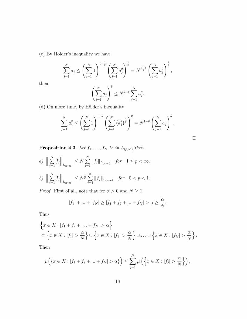
(c) By Holder’s inequality we have

N∑j=1

aj ≤

(N∑j=1

1

)1− 1θ(

N∑j=1

aθj

) 1θ

= Nθ−1θ

(N∑j=1

aθj

) 1θ

,

then (N∑j=1

aj

)θ

≤ N θ−1N∑j=1

aθj .

(d) On more time, by Holder’s inequality

N∑j=1

aθj ≤

(N∑j=1

1

)1−θ( N∑j=1

(aθj) 1θ

)θ

= N1−θ

(N∑j=1

aj

)θ

.

Proposition 4.3. Let f1, . . . , fN be in L(p,∞) then

a)∥∥∥ N∑j=1

fj

∥∥∥L(p,∞)

≤ NN∑j=1

‖fj‖L(p,∞)for 1 ≤ p <∞.

b)∥∥∥ N∑j=1

fj

∥∥∥L(p,∞)

≤ N1p

N∑j=1

‖fj‖L(p,∞)for 0 0 and N ≥ 1

|f1|+ ...+ |fN | ≥ |f1 + f2 + ...+ fN | > α ≥ α

N.

Thus{x ∈ X : |f1 + f2 + . . .+ fN | > α

}⊂{x ∈ X : |f1| >

α

N

}∪{x ∈ X : |f1| >

α

N

}∪ . . . ∪

{x ∈ X : |fN | >

α

N

}.

Then

µ({x ∈ X : |f1 + f2 + ...+ fN | > α}

)≤

N∑j=1

µ({x ∈ X : |fj| >

α

N

}),

18

that is

D∑ fj(α) ≤N∑j=1

Dfj

( αN

).

Hence

∥∥∥ N∑j=1

fj

∥∥∥pL(p,∞)

= supα>0

αpD∑ fj(α) ≤N∑j=1

supα>0

αpDfj

( αN

)=

N∑j=1

supα>0

αpDNfj(α)

=N∑j=1

‖Nfj‖pL(p,∞)= Np

N∑j=1

‖fj‖pL(p,∞),

thus

∥∥∥ N∑j=1

fj

∥∥∥L(p,∞)

≤ N

(N∑j=1

‖fj‖pL(p,∞)

) 1p

.

By proposition (4.2) (a) since 0 < 1p< 1 we have

∥∥∥ N∑j=1

fj

∥∥∥L(p,∞)

≤ N

(N∑j=1

‖fj‖L(p,∞)

).

(b) As in part (a) we have∥∥∥ N∑j=1

fj

∥∥∥pL(p,∞)

≤ Np

(N∑j=1

∥∥fj∥∥pL(p,∞)

).

Since 0 < p < 1, then 1 < 1p, next by proposition 4.2 (c) we have

∥∥∥ N∑j=1

fj

∥∥∥L(p,∞)

≤ N

(N∑j=1

∥∥fj∥∥pL(p,∞)

) 1p

≤ N(N1p−1)

N∑j=1

(∥∥fj∥∥pL(p,∞)

) 1p

= N1p

N∑j=1

∥∥fj∥∥L(p,∞).

19

Proposition 4.4. Give a measurable function f on (X,µ) and λ > 0, definefλ = fχ{|f |>λ} and fλ = f − fλ = fλ = fχ{|f |≤λ}.

a) Then

Dfλ(α) =

{Df (α) when α > λDf (λ) when α ≤ λ.

Dfλ(α) =

{0 when α ≥ λ

Df (α)−Df (λ) when α < λ

b) If f ∈ Lp(X,µ). Then

∥∥fλ∥∥pLp = p

∞∫λ

αp−1Df (α) dα + λpDf (λ),

∥∥fλ∥∥pLp

= p

λ∫0

αp−1Df (α) dα− λpDf (λ),

∫λ<|f |≤δ

|f |p dµ = p

δ∫λ

αp−1Df (α) dα− δpDf (α) + λpDf (λ).

c) If f is in L(p,∞) then fλ is in Lq(X,µ) for any q > p and fλ is in Lq(X,µ)for any q < p. Thus L(p,∞) ⊆ Lp0+Lp1 when 0 < p0 λ}(x) > α}

)= µ

({x : |f(x)| > α}∩{x : |f | > λ}

),

if α > λ, then {x : |f(x)| > α} ⊆ {x : |f | > λ}, thus

Dfλ(α) = µ({x : |f(x)| > α}∩{x : |f | > λ}

)= µ

({x : |f(x)| > α}

)= Df (α).

If α ≤ λ, then {x : |f(x)| > λ} ⊆ {x : |f | > α}, thus

Dfλ(α) = µ({x : |f(x)| > α}∩{x : |f | > λ}

)= µ

({x : |f(x)| > λ}

)= Df (λ).

20

And thus

Dfλ(α) =

{Df (α) when α > λDf (λ) when α ≤ λ.

(20)

Next, consider

Dfλ(α) = µ({x : |f(x)|χ{|f |≤λ}(x) > α}

)= µ

({x : |f(x)| > α} ∩ {x : |f | ≤ λ}

),

if α ≥ λ then {x : |f | > α} ∩ {x : |f(x)| ≤ λ} = ∅, thus Dfλ(α) = 0.If α < λ, then

Dfλ(α) = µ({x : |f(x)| > α} ∩ {x : |f(x)| ≤ λ}

)= µ

({x : |f(x)| > α} ∩ {x : |f(x)| > λ}c

)= µ

({x : |f(x)| > α}\{x : |f(x)| > λ}

)= µ

({x : |f(x)| > α}

)− µ

({x : |f(x)| > λ}

)= Df (α)−Df (λ).

And hence

Dfλ(α) =

{0 when α ≥ λ

Df (α)−Df (λ) when α < λ.(21)

(b) If f ∈ Lp(X,µ), then


∞∫0

αp−1Dfλ(α) dα = p

λ∫0

αp−1Dfλ(α) dα + p

∞∫λ

αp−1Dfλ(α) dα,

By part (a)(20) we have


λ∫0

αp−1Df (λ) dα + p

∞∫λ

αp−1Df (α) dα

= λpDf (λ) + p

∞∫λ

αp−1Df (α) dα.

21

Also

∥∥fλ∥∥pLp

= p

∞∫0

αp−1Dfλ(α) dα = p

λ∫0

αp−1Dfλ(α) dα + p

∞∫λ

αp−1Dfλ(α) dα,

by part (a) (21) we obtain

∥∥fλ∥∥pLp

= p

λ∫0

αp−1(Df (α)−Df (λ)

)dα = p

λ∫0

αp−1Df (α) dα− λpDf (λ).

Next,∫λ<|f |≤δ

|f |p dµ

=

∫|f |>λ

|f |p dµ−∫|f |>δ

|f |p dµ

=

∫X

|f |pχ{|f |>λ} dµ−∫X

|f |pχ{|f |>δ} dµ

=

∫X

|fλ|p dµ−∫X

|fδ|p dµ

= p

∞∫λ

αp−1Df (α) dα + λpDf (λ)− p∞∫δ

αp−1Df (α) dα− δpDf (δ)

= p

∞∫λ

αp−1Df (α) dα−∞∫δ

αp−1Df (α) dα

+ λpDf (λ)− δpDf (δ)

= p

δ∫λ

αp−1Df (α) dα− δpDf (α) + λpDf (λ).

(c) We known that

Df (α) ≤

∥∥f∥∥pL(p,∞)

αp,

then if q > p

22

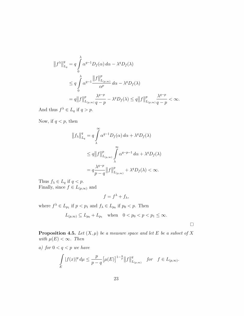
∥∥fλ∥∥qLq

= q

λ∫0

αq−1Df (α) dα− λqDf (λ)

≤ q

λ∫0

αq−1

∥∥f∥∥pL(p,∞)

αpdα− λqDf (λ)

= q∥∥f∥∥p

L(p,∞)

λq−p

q − p− λqDf (λ) ≤ q

∥∥f∥∥pL(p,∞)

λq−p

q − p<∞.

And thus fλ ∈ Lq if q > p.

Now, if q < p, then

∥∥fλ∥∥qLq = q

∞∫λ

αq−1Df (α) dα + λqDf (λ)

≤ q∥∥f∥∥p

L(p,∞)

∞∫λ

αq−p−1 dα + λqDf (λ)

= qλq−p

p− q∥∥f∥∥p

L(p,∞)+ λqDf (λ) <∞.

Thus fλ ∈ Lq if q < p.Finally, since f ∈ L(p,∞) and

f = fλ + fλ,

where fλ ∈ Lp1 if p < p1 and fλ ∈ Lp0 if p0 < p. Then

L(p,∞) ⊆ Lp0 + Lp1 when 0 < p0 < p < p1 ≤ ∞.

Proposition 4.5. Let (X,µ) be a measure space and let E be a subset of Xwith µ(E) <∞. Then

a) for 0 < q < p we have∫E

|f(x)|q dµ ≤ p

p− q[µ(E)

]1− qp∥∥f∥∥q

L(p,∞)for f ∈ L(p,∞).

23

b) Conclude that if µ(X) <∞ and 0 < q < p, then

Lp(X,µ) ⊆ L(p,∞) ⊆ Lq(X,µ).

Proof. Let f ∈ L(p,∞), then∫E

|f |q dµ

= q

∞∫0

λq−1µ({x ∈ E : |f(x)| > λ}

)dλ

≤ q

[µ(E)]− 1

p ‖f‖L(p,∞)∫0

λq−1µ(E) dλ+ q

∞∫[µ(E)]− 1

p ‖f‖L(p,∞)

λq−1Df (λ) dλ

≤ q

[µ(E)]− 1

p ‖f‖L(p,∞)∫0

λq−1µ(E) dλ+ q

∞∫[µ(E)]− 1

p ‖f‖L(p,∞)

λq−1‖f‖pL(p,∞)

λpdλ

=([µ(E)

]− 1p‖f‖L(p,∞)

)qµ(E) +

q

p− q

([µ(E)

]− 1p‖f‖L(p,∞)

)q−p‖f‖pL(p,∞)

=[µ(E)

]1− qp‖f‖qL(p,∞)

+q

p− q[µ(E)

]1− qp‖f‖qL(p,∞)

=p

p− q[µ(E)

]1− qp‖f‖qL(p,∞)

.

And thus ∫E

|f |q dµ ≤ p

p− q[µ(E)

]1− qp∥∥f∥∥q

L(p,∞).

(b) If µ(X) <∞, then∫X

|f |q dµ ≤ p

p− q[µ(X)

]1− qp∥∥f∥∥q

L(p,∞).

24

HenceLp ⊆ L(p,∞) ⊆ Lq.

Corolario 4.1. Let (X,µ) be a measurable space and let E be a subset of Xwith µ(E) <∞. Then

‖f‖p/2 ≤[4µ(E)

]1/p∥∥f∥∥L(p,∞)

.

And thus L(p,∞) ⊆ Lp/2.

Proof. Since 0 < p2< p we can apply proposition 4.5 to obtain∫

E

|f |p/2 dµ ≤ p

p− p2

[µ(E)]1−p/2p

∥∥f∥∥p/2L(p,∞)

= 2[µ(E)]1/2∥∥f∥∥p/2

L(p,∞)

‖f‖p/2 ≤ 22/p[µ(E)]1/p∥∥f∥∥

L(p,∞)

=[4µ(E)

]1/p∥∥f∥∥L(p,∞)

.

From this last result one can see that

L(p,∞) ⊆ Lp/2.

5 Normability of Weak Lp for p > 1

Let (X,A, µ) be a measure space and let 0 < p < ∞. Pick 0 < r < p anddefine ∣∣∣∣∣∣f ∣∣∣∣∣∣

L(p,∞)= sup

0<µ(E)<∞

[µ(E)

]− 1r+ 1p

∫E

|f |r dµ

1r

,

where the supremum is taken over all measurable subsets E of X of finitemeasure.

25

Proposition 5.1. Let f be in L(p,∞). Then

∥∥f∥∥L(p,∞)

≤∣∣∣∣∣∣f ∣∣∣∣∣∣

L(p,∞)≤(

p

p− r

) 1r ∥∥f∥∥

L(p,∞).

Proof. By proposition 4.5 with q = r we have

∣∣∣∣∣∣f ∣∣∣∣∣∣L(p,∞)

= sup0<µ(E)<∞

[µ(E)

]− 1r+ 1p

∫E

|f |r dµ

1r

≤ sup0<µ(E)<∞

[µ(E)

]− 1r+ 1p

(p

p− r[µ(E)

]1− rp∥∥f∥∥r

L(p,∞)

) 1r

= sup0<µ(E)<∞

[µ(E)

]− 1r+ 1p

(p

p− r

) 1r [µ(E)

] 1r− 1p∥∥f∥∥

L(p,∞)

=

(p

p− r

) 1r ∥∥f∥∥

L(p,∞).

On the other hand by definition

[µ(E)

]− 1r+ 1p

∫E

|f |r dµ

1r

≤∣∣∣∣∣∣f ∣∣∣∣∣∣

L(p,∞),

for all E ∈ A such that µ(E) <∞ now, let us consider A = {x : |f(x)| > α}for f ∈ L(p,∞). Observe that µ(A) <∞. Then

∣∣∣∣∣∣f ∣∣∣∣∣∣pL(p,∞)

≥

[µ(A)]− 1

r+ 1p

∫A

|f |r dµ

1r

p

≥[Df (α)

]− pr+1

∫A

αr dµ

pr

=[Df (α)

]− pr+1αp[Df (α)

] pr = αpDf (α).

That isαpDf (α) ≤

∣∣∣∣∣∣f ∣∣∣∣∣∣L(p,∞)

,

26

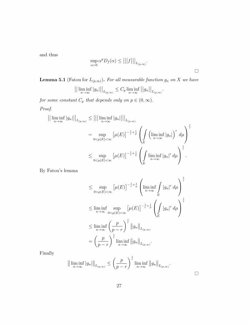
and thussupα>0

αpDf (α) ≤∣∣∣∣∣∣f ∣∣∣∣∣∣

L(p,∞).

Lemma 5.1 (Fatou for L(p,∞)). For all measurable function gn on X we have∣∣∣∣ lim infn→∞

|gn|∣∣∣∣L(p,∞)

≤ Cp lim infn→∞

∣∣∣∣gn∣∣∣∣L(p,∞).

for some constant Cp that depends only on p ∈ (0,∞).

Proof.∣∣∣∣ lim infn→∞

|gn|∣∣∣∣L(p,∞)

≤∣∣∣∣∣∣ lim inf

n→∞|gn|∣∣∣∣∣∣

L(p,∞)

= sup0<µ(E)<∞

[µ(E)

]− 1r+ 1p

∫E

(lim infn→∞

|gn|)r

dµ

1r

≤ sup0<µ(E)<∞

[µ(E)

]− 1r+ 1p

∫E

lim infn→∞

|gn|r dµ

1r

.

By Fatou’s lemma

≤ sup0<µ(E)<∞

[µ(E)

]− 1r+ 1p

lim infn→∞

∫E

|gn|r dµ

1r

≤ lim infn→∞

sup0<µ(E)<∞

[µ(E)

]− 1r+ 1p

∫E

|gn|r dµ

1r

≤ lim infn→∞

(p

p− r

) 1r ∥∥gn∥∥L(p,∞)

=

(p

p− r

) 1r

lim infn→∞

∥∥gn∥∥L(p,∞).

Finally ∥∥ lim infn→∞

|gn|∥∥L(p,∞)

≤(

p

p− r

) 1r

lim infn→∞

∥∥gn∥∥L(p,∞).

27

The following result is an improvement of lemma 5.1.

Lemma 5.2. For all measurable functions gn on X we have∥∥ lim infn→∞

|gn|∥∥L(p,∞)

≤ lim infn→∞

∥∥gn∥∥L(p,∞).

Proof. SinceDlim inf

n→∞|gn|(λ) ≤ lim inf

n→∞Dgn(λ),

Then{C > 0 : lim inf

n→∞Dgn(λ) ≤ Cp

λp

}⊆{C > 0 : Dlim inf

n→∞|gn|(λ) ≤ Cp

λp

},

and thus∥∥ lim infn→∞

|gn|∥∥L(p,∞)

= inf

{C > 0 : Dlim inf

n→∞|gn|(λ) ≤ Cp

λp

}≤ inf

{C > 0 : lim inf

n→∞Dgn(λ) ≤ Cp

λp

}= lim inf

n→∞

(inf

{C > 0 : Dgn(λ) ≤ Cp

λp

})= lim inf

n→∞

∥∥gn∥∥L(p,∞).

Proposition 5.2. Let 0 < p < 1, 0 < s <∞ and (X,A, µ) be a measurablespace

a) Let f be a measurable function on X. Then∫{|f |≤s}

|f | dµ ≤ s1−p

1− p∥∥f∥∥p

L(p,∞).

b) Let fj, 1 ≤ j ≤ m, be measurable functions on X. Then

∥∥ max1≤j≤m

|fj|∥∥pL(p,∞)

≤m∑j=1

∥∥fj∥∥pL(p,∞).

And also

28

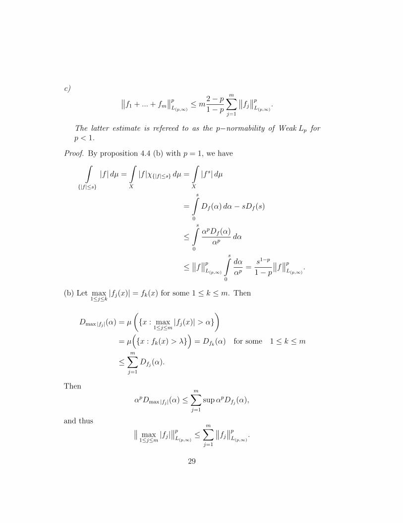
c) ∥∥f1 + ...+ fm∥∥pL(p,∞)

≤ m2− p1− p

m∑j=1

∥∥fj∥∥pL(p,∞).

The latter estimate is refereed to as the p−normability of Weak Lp forp < 1.

Proof. By proposition 4.4 (b) with p = 1, we have∫{|f |≤s}

|f | dµ =

∫X

|f |χ{|f |≤s} dµ =

∫X

|f s| dµ

=

s∫0

Df (α) dα− sDf (s)

≤s∫

0

αpDf (α)

αpdα

≤∥∥f∥∥p

L(p,∞)

s∫0

dα

αp=

s1−p

1− p∥∥f∥∥p

L(p,∞).

(b) Let max1≤j≤k

|fj(x)| = fk(x) for some 1 ≤ k ≤ m. Then

Dmax |fj |(α) = µ

({x : max

1≤j≤m|fj(x)| > α}

)= µ

({x : fk(x) > λ}

)= Dfk(α) for some 1 ≤ k ≤ m

≤m∑j=1

Dfj(α).

Then

αpDmax |fj |(α) ≤m∑j=1

supαpDfj(α),

and thus ∥∥ max1≤j≤m

|fj|∥∥pL(p,∞)

≤m∑j=1

∥∥fj∥∥pL(p,∞).

29

(c) Observe that

max1≤j≤m

|fj| ≤ |f1|+ |f2|+ ...+ |fm|,

from this we have{x : max

1≤j≤m|fj(x)| > α

}⊂{x : |f1|+ ...+ |fm| > α

},

then {x : |f1|+ ...+ |fm| > α

}=

({x : |f1|+ ...+ |fm| > α

}∩{x : max

1≤j≤m|fj(x)| ≤ α

})∪{x : max

1≤j≤m|fj(x)| > α

}.

And thus

Df1+...+fm(α) = µ({x : |f1 + ...+ fm| > α}

)≤ µ

({x : |f1|+ ...+ |fm| > α}

)≤ µ

({x : |f1|+ ...+ |fm| > α} ∩ {x : max

1≤j≤m|fj(x)| ≤ α}

)+ µ

({x : max

1≤j≤m|fj(x)| > α}

)= µ

({x ∈ {x : max

1≤j≤m|fj(x)| ≤ α} : |f1|+ ...+ |fm| > α

})+ µ

({x : max

1≤j≤m|fj(x)| > α}

)= µ

({x :(|f1|+ ...+ |fm|

)χ{x:max |fj |≤α} > α

})+ µ

({x : max

1≤j≤m|fj(x)| > α}

).

30

By Chebyshev’s inequality

Df1+...+fm(α) ≤ 1

α

∫{x:max |fj |≤α}

(|f1|+ ...+ |fm|

)dµ+Dmax |fj |(α)

=m∑j=1

1

α


|fj| dµ+Dmax |fj |(α)

≤m∑j=1

1

α


max1≤j≤m

|fj| dµ+Dmax |fj |(α).

By part (a) we have

m∑j=1

1

α


max1≤j≤m

|fj| dµ+Dmax |fj |(α)

≤m∑j=1

1

α

α1−p

1− p

∥∥∥ max1≤j≤m

|fj|∥∥∥pL(p,∞)

+

∥∥ max1≤j≤m

|fj|∥∥pL(p,∞)

αp

≤m∑j=1

α−p

1− p

∥∥∥ max1≤j≤m

|fj|∥∥∥pL(p,∞)

+m∑j=1

∥∥ max1≤j≤m

|fj|∥∥pL(p,∞)

αp.

Finally by part (b) we obtain

αpDf1+...+fm(α) ≤m∑j=1

( 1

1− p+ 1)∥∥∥ max

1≤j≤m|fj|∥∥∥pL(p,∞)

=m∑j=1

(2− p1− p

)∥∥∥ max1≤j≤m

|fj|∥∥∥pL(p,∞)

≤ 2− p1− p

m∑j=1

m∑j=1

∥∥fj∥∥pL(p,∞)

= m2− p1− p

m∑j=1

∥∥fj∥∥pL(p,∞).

31

Proposition 5.3 (Lyapunov’s inequality for Weak Lp). Let (X,µ) be mea-surable space. Suppose that 0 < p0 < p < p1 <∞ and 1

p= 1−θ

p0+ θ

p1for some

θ ∈ [0, 1]. If f ∈ L(p0,∞) ∩ L(p1,∞) then f ∈ L(p,∞) and∥∥f∥∥L(p,∞)

≤∥∥f∥∥1−θ

L(p0,∞)

∥∥f∥∥θL(p1,∞)

.

Proof. Observe that

αpDf (α) = αp(1−θ+θ)[Df (α)

]p(1p

)

= αp(1−θ)αpθ[Df (α)

]p(1−θp0

+θp1

)

= αp(1−θ)[Df (α)

]p(1−θp0

)αpθ[Df (α)

]pθp1

=[αp0Df (α)

]p(1−θp0

)[αp1Df (α)

]pθp1 .

Thus

αpDf (α) ≤[supα>0

αp0Df (α)

]p(1−θp0

) [supα>0

αp1Df (α)

]pθp1

αpDf (α) ≤[∥∥f∥∥p0

L(p0,∞)

]p(1−θp0

) [∥∥f∥∥p1L(p1,∞)

]pθp1 ,

finally

supα>0

αpDf (α) ≤[∥∥f∥∥p0

L(p0,∞)

]p(1−θp0

) [∥∥f∥∥p1L(p1,∞)

]pθp1

∥∥f∥∥pL(p,∞)

≤[∥∥f∥∥1−θ

L(p0,∞)

∥∥f∥∥θL(p1,∞)

]p∥∥f∥∥

L(p,∞)≤∥∥f∥∥1−θ

L(p0,∞)

∥∥f∥∥θL(p1,∞)

.

32

Theorem 5.1 (Holder’s inequality for Weak spaces). Let fj be in L(pj ,∞)

where 0 < pj <∞ and 1 ≤ j ≤ k. Let

1

p=

1

p1+ ...+

1

pk.

Then ∥∥f1...fk∥∥L(p,∞)≤ p−

1p

k∏j=1

p1pj

j

k∏j=1

∥∥fj∥∥L(pj,∞).

Proof. Let us consider∥∥fj∥∥L(pj,∞)

= 1, 1 ≤ j ≤ k. And let x1, . . . , xn be a

positive real numbers such that

1

x1. . .

1

xk= α,

then

Df1...fk(α) = Df1...fk

(1

x1. . .

1

xk

)

≤ Df1

(1

x1

)+Df2

(1

x2

)+ . . .+Dfk

(1

xk

), (22)

since

1 =∥∥fj∥∥pjL(pj,∞)

≥ supj

(1

xj

)pjDfj

(1

xj

),

then (1

xj

)pjDfj

(1

xj

)≤ 1,

thus

Dfj

(1

xj

)≤ x

pjj for 1 ≤ j ≤ k.

Hence, we can write (22) as follows

Df1...fk

(1

x1. . .

1

xk

)≤ xp11 + xp22 + . . .+ xpkk .

33

Next, let us define

F (x1, . . . , xk) = xp11 + xp22 + . . .+ xpkk .

In what follows, we will use the Lagrange multipliers in order to obtain theminimum value of F subject to the constrain

1

x1. . .

1

xk= α.

That isf(x1, x2, . . . , xk) = xp11 + xp22 + . . .+ xpkk

g(x1, x2, . . . , xk) = x1x2 . . . xk −1

α.

Then, next∇F = λ∇g.

And thusp1x

p1−11 = λ(x2x3 . . . xk)

p2xp2−12 = λ(x1x3 . . . xk)

...

pjxpj−1j = λ(x1x3 . . . xk),

thusp1x

p11 = λ(x1x2 . . . xk)

p2xp22 = λ(x1x2 . . . xk)

...

pjxpjj = λ(x1x2 . . . xk).

Observe that

x1x2 . . . xk =1

α. (23)

On the other hand note that

p1xp11 = pjx

pjj for 2 ≤ j ≤ k. (24)

34

Now replacing (24) into (23) we have

x1

(p1p2

) 1p2

xp1p21

(p1p3

) 1p3

xp1p3 . . .

(p1pk

) 1pk

xp1pk1

= x1

(p1p2

) 1p2

(p1p3

) 1p3

. . .

(p1pk

) 1pk

xp1p2

+p1p3

+...+p1pk

1 =1

α, (25)

but (p1p1

) 1p1

= 1,

then we can write (25) as follows(p1p1

) 1p1

(p1p2

) 1p2

(p1p3

) 1p3

. . .

(p1pk

) 1pk

xp1p1

+p1p2

+p1p3

+...+p1pk

1 =1

α.

And, thus

p1p1

+ 1p2

+...+ 1pk

1

k∏j=1

p1pj

j

xp1(

1p1

+ 1p2

+...+ 1pk

)1 =

1

α.

Then

p1p

1 xp1p =

k∏j=1

p1pj

j

α,

hence

xp11 =1

p1αp

[k∏j=1

p1pj

j

]p.

Therefore the x1 . . . xk such thatxp11 =

1

p1αp

[k∏j=1

p1pj

j

]p

xpjj =

p1pjxp11

(26)

are the unique critical real point.

35

For this critical real point, using (26) we have

xp11 + xp22 + . . .+ xpkk = xp11 +p1p2xp11 + . . .+

p1pkxp11

= p1xp11

[1

p1+ . . .+

1

pk

]

=1

αp

[k∏j=1

p1pj

j

]p1

p.

On the other hand observe that one can make the function

F (x1, . . . , xk) = xp11 + . . .+ xpkk ,

subject to the constrain

x1x2 . . . xk =1

α,

as big as one wish. Indeed if x1 = Mα

, x2 = 1M

and xj = 1 for 3 ≤ j ≤ k.Then

F (x1, . . . , xk) = xp11 + xp22 + . . .+ xpkk

=

(M

α

)p1+

(1

M

)p1+ 1 + . . .+ 1

=

(M

α

)p1+

(1

M

)p1+ k − 2→∞,

as M →∞, therefore the critical part (26) is a minimum. Then

Df1...fk(α) ≤ 1

pαp

[k∏j=1

p1pj

j

]p

αpDf1...fk(α) ≤ 1

p

[k∏j=1

p1pj

j

]p,

36

thus, we have

αpDf1...fk(α) ≤ 1

p

[k∏j=1

p1pj

j

]p

∥∥f1 . . . fk∥∥L(p,∞)≤(

1

p

) 1p

(k∏j=1

p1pj

j

)k∏j=1

∥∥fj∥∥L(pj,∞), (27)

since∥∥fj∥∥L(pj,∞)

= 1.

In general, if∥∥fj∥∥L(pj,∞)

6= 1, 1 ≤ j ≤ k choose gj =fj

‖fj‖L(pj,∞)

and use (27)

Theorem 5.2 (Completeness). Weak Lp with the quasi-norm ‖.‖L(p,∞)is

complete for all 0 0 there exists an n0 ∈ N such that

‖fn − fm‖L(p,∞)< ε

1p+1

if m,n ≥ n0, that is,(supλ>0

λpDfn−fm(λ)

)1/p

= ‖fn − fm‖L(p,∞)< ε

1p+1,

taking λ = ε we have

εpµ({x ∈ X : |fn(x)− fm(x)| > ε}

)< εp+1,

for m,n ≥ n0. Hence

µ({x ∈ X : |fn(x)− fm(x)| > ε}

)< ε,

for m,n ≥ n0. This means that {fn}n∈N is a Cauchy sequence in the mea-sure µ. We therefore apply theorem 3.2 and conclude that there exists anA−measurable function f such that some subsequence of {fn}n∈N converges

37

to f µ−a.e. Let {fnk}k∈N be such subsequence of {fn}n∈N of {fn}n∈N thenfnk → f µ-a.e as k →∞. If we apply twice lemma 5.2 we obtain firstly∥∥f∥∥

L(p,∞)=∥∥ lim inf |fnk |

∥∥L(p,∞)

≤ lim inf∥∥fnk∥∥L(p,∞)

<∞,

thus f ∈Weak Lp.Secondly ∥∥f − fn∥∥L(p,∞)

=∥∥ lim inf |fnk − fn|

∥∥L(p,∞)

≤ lim inf∥∥fnk − fn∥∥L(p,∞)

< ε1p+1,

if nk, n ≥ n0.This prove that Weak Lp is complete for 0 < p <∞.

38

6 Multiplication Operators

Let F (X) be a function space on non-empty set X. Let u : X → C be afunction such that u.f on F (X) whenever f ∈ F (X).Then the transformation f → u.f on F (X) is denoted by Mu. In case F (X)is a topological space and Mu is continuous, we call it a multiplication oper-ator induced by u.

In this section boundedness and invertibility of the multiplication Mu arecharacterized in terms of the boundedness and invertibility of the complex-valued measurable function u respectively.

Theorem 6.1. The linear transformation Mu : f → u.f on the Weak Lpspaces is bounded if only if u is essentially bounded. Moreover∥∥Mu

∥∥ = ‖u‖∞.

Proof. Let u ∈ L∞(u), then we find

∥∥Muf∥∥L(p,∞)

= supλ>0

λ[DMuf (λ)

]1/p= sup

λ>0λ[µ({x ∈ X : |Muf(x)| > λ}

)]1/p= sup

λ>0λ[µ({x ∈ X : |(u.f)(x)| > λ}

)]1/p≤ sup

λ>0λ[µ({

x ∈ X : |f(x)| > λ‖u‖∞

})]1/p.

Since{x ∈ X : |(u.f)(x)| > λ

}⊂{x ∈ X : ‖u‖∞|f(x)| > λ

}={x ∈ X : |f(x)| > λ

‖u‖∞

}.

39

Putting α =λ

‖u‖∞we have

supλ>0

λ[µ({

x ∈ X : |f(x)| > λ‖u‖∞

})]1/p= sup

α>0α‖u‖∞

[µ({x ∈ X : |f(x)| > α}

)]1/p= ‖u‖∞ sup

α>0α[µ({x ∈ X : |f(x)| > α}

)]1/p= ‖u‖∞

∥∥f∥∥L(p,∞)

.

Hence, we have proved that∥∥Muf∥∥L(p,∞)

≤ ‖u‖∞∥∥f∥∥

L(p,∞). (28)

Conversely, supposeMu is a bounded operator. If u is not essentially boundedfunction, then for every n ∈ N, the set En =

{x ∈ X : |u(x)| > n

}has

positive measure and note that{x ∈ X : nχEn(x) > λ

}⊂{x ∈ X : |uχEn(x)| > λ

},

then

supλ>0

λ[µ({x ∈ X : nχEn(x) > λ}

)]1/p≤ sup

λ>0λ[µ({x ∈ X : |uχEn(x)| > λ}

)]1/p.

Thusn∥∥χEn∥∥L(p,∞)

≤∥∥MuχEn

∥∥L(p,∞)

.

This contradicts the boundedness of Mu.

Clearly from (28) we have ∥∥Mu

∥∥ ≤ ‖u‖∞. (29)

Next, for ε > 0, let

E ={x ∈ X : |u(x)| > ‖u‖∞ − ε

}.

40

Note µ(E) > 0. Then{x ∈ X :

(‖u‖∞ − ε

)χE(x) > λ

}⊂{x ∈ X : |uχE(x)| > λ

},

and thus

supλ>0

λ[µ({

x ∈ X :(‖u‖∞ − ε

)χE(x) > λ

})]1/p≤ sup

λ>0λ[µ({x ∈ X : |uχEn(x)| > λ}

)]1/p.

Therefore (‖u‖∞ − ε

)∥∥χE∥∥L(p,∞)≤∥∥MuχE

∥∥L(p,∞)

‖u‖∞ − ε ≤

∥∥MuχE∥∥L(p,∞)∥∥χE∥∥L(p,∞)

≤∥∥Mu

∥∥.Thus

‖u‖∞ ≤∥∥Mu

∥∥, (30)

finally from (29) and (30) ∥∥Mu

∥∥ = ‖u‖∞.

Theorem 6.2. The set of all multiplication operator on WeakLp‘is an maximal-abelian subalgebra of the set B (Weak Lp), the algebra of all bounded linearoperation on Weak Lp.

Proof. Let

H ={Mu : u ∈ L∞

},

and consider the operator product

Mu.Mv = Muv,

where Mu, Mv ∈ H, let us check that H is a Banach algebra. Lea u, v ∈ L∞then |u| ≤ ‖u‖∞ and |v| ≤ ‖v‖∞ therefore:

‖uv‖∞ ≤ ‖v‖∞‖u‖∞,

41

this implies that product is an inner operation, moreover the usual func-tion product is associative, commutative and distributive with respect to thesum and the scalar product, thus we conclude that H is a subalgebra ofB (Weak Lp).

Now, we like to check that H is a maximal subalgebra, that is, given N ∈B (Weak Lp), if N commute with H we have to prove that N ∈ H.

Consider the unit function e : X → C defined by e(x) = 1 for all x ∈ X letN ∈ B (Weak Lp) be an operator which commute with H and let χE be thecharacteristic function of a measurable set E. Then

N(χE) = N [MχE(e)]

= MχE [N(e)]

= χE.N(e)

= N(e).χE

= Mw(χE),

where w = N(e). Similarly

N(s) = Mw(s), (31)

for any simple function.Now, let us check that w ∈ L∞. By way of contradiction assume thatw /∈ L∞, then the set

En ={x ∈ X : |w(x)| > n

},

has a positive measure for each n ∈ N. Note that:

Mw(χEn)(x) =(wχEn

)(x) ≥ nχEn(x),

for all x ∈ X. By the monotonicity (Property 1) of the distribution function,we have

DwχEn(λ) ≥ DχEn

(λ

n

),

thus

supλ>0

λpDwχEn(λ) ≥ sup

λ>0λpDχEn

(λ

n

),

42

Putting α = λn

we have∥∥wχEn∥∥pL(p,∞)= sup

λ>0λpDwχEn

(λ) ≥ np supα>0

αpDχEn(α)

= np∥∥χEn∥∥pL(p,∞)

,

since χEn is a simple function then by (31) we have

Mw(χEn) = N(χEn),

Hence ∥∥N(χEn)∥∥L(p,∞)

≥ n∥∥χEn∥∥L(p,∞)

,

Therefore N is a unbounded operator. This is a contradiction to the fact Nis bounded.So then w ∈ L∞ and by theorem 6.1 Mw is bounded.

Next, given f ∈WeakLp there exists a nondecreasing sequence {sn}n∈N of ameasurable simple functions such that lim

n→∞sn = f , then by (31) we have

N(f) = N(

limn→∞

sn

)= lim

n→∞N(sn) = lim

n→∞Mw(sn)

= Mw

(limn→∞

sn

)= Mw(f).

Therefore, N(f) = Mw(f) for all f ∈ Weak Lp and thus we conclude thatN ∈ H.

Corolario 6.1. The multiplication operator Mu is invertible if only if u isinvertible on L∞.

Proof. Let Mu be invertible, the there exists N ∈ B(Weak Lp

)such that:

Mu.N = N.Mu = I, (32)

where I represent the identity operator. Let us check that N commute withH. Let Mw ∈ H, then:

Mw.Mu = Mu.Mw. (33)

43

Applying N to (33) and by (32) we obtain:

N.Mw.Mu.N = N.Mu.Mw.N,

N.Mw.I = I.Mw.N,

N.Mw = Mw.N,

and thus we concluded that N commute with H, by theorem 6.2 N ∈ H

then there exists g ∈ L∞ such that N = Mg, hence

Mu.Mg = Mg.Mu = I,

this implies that ug = gu = 1, a.e[µ] this means that u is invertible on L∞.

On the other hand, assume u is invertible on L∞ that is,1

u∈ L∞, then:

Mu.M1/u = M1/u.Mu = M(1/u)u

= M1 = I,

which means that Mu is invertible on B (Weak Lp).

Lemma 6.1. Let Mu be a compact operator, for ε > 0 define

Aε(u) ={x ∈ X : |u(x)| ≥ ε

},

andWeak Lp

[Aε(u)

]={fχAε(u) : f ∈Weak Lp

}.

Then Weak Lp[Aε(u)

]is a closed invariant subspace of Weak Lp under Mu.

Moreover

Mu

∣∣∣Weak Lp[Aε(u)]

,

is a compact operator.

Proof. Let h, s ∈ Weak Lp[Aε(u)

]and α, β ∈ R. Then h = fχAε(u) and

s = gχAε(u) where f, g ∈Weak Lp, thus

αh+ βs = α(fχAε(u)

)+ β

(gχAε(u)

)= (αf + βg)χAε(u) ∈Weak Lp

[Aε(u)

].

44

Which mean that Weak Lp[Aε(u)

]is a subspace of Weak Lp.

Next, for all h ∈Weak Lp[Aε(u)

]we have

Muh = uh = ufχAε(u)

= (uf)χAε(u),

where uf ∈Weak Lp.Therefore, Muh ∈Weak Lp

[Aε(u)

], which means that Weak Lp

[Aε(u)

]is an

invariant subspace of Weak Lp under Mu.

Now, let us show that Weak Lp[Aε(u)

]is a closed set. Indeed, let g be

a function belonging to the closure of Weak Lp[Aε(u)

]then there exists a

sequence {gn}n∈N in Weak Lp[Aε(u)

]such that

gn → g,

in Weak Lp. Just remain to exhibit that g belong to Weak Lp[Aε(u)

]. Note

thatg = gχAε(u) + gχAcε(u).

Next, we want to show that gχAcε(u) = 0. In fact, given ε1 > 0 there existsn0 ∈ N such that∥∥gχAcε(u)∥∥L(p,∞)

=∥∥(g − gn0 + gn0)χAcε(u)

∥∥L(p,∞)

=∥∥(g − gn0)χAcε(u)

∥∥L(p,∞)

≤∥∥g − gn0

∥∥L(p,∞)

< ε1.

Thus gχAcε(u) = 0, which mean that g = gχAε(u) that is g ∈Weak Lp[Aε(u)

].

And the proof is now complete.

Theorem 6.3. Let Mu ∈ B (Weak Lp). Then Mu is compact if and only ifWeak Lp

[Aε(u)

]is finite dimensional for each ε > 0.

Proof. If |u(x)| ≥ ε, we should note that∣∣ufχAε(u)(x)∣∣ ≥ εfχAε(u)(x),

and thus{x ∈ X : εfχAε(u)(x) > λ

}⊂{x ∈ X :

∣∣ufχAε(u)(x)∣∣ > λ

},

45

thenDufχAε(u)

(λ) ≥ DεfχAε(u)(λ)

λ[DufχAε(u)

(λ)]1/p ≥ λ

[DεfχAε(u)

(λ)]1/p

supλ>0

λ[DufχAε(u)

(λ)]1/p ≥ sup

λ>0λ[DεfχAε(u)

(λ)]1/p∥∥ufχAε(u)∥∥L(p,∞)≥∥∥εfχAε(u)∥∥L(p,∞)

= ε∥∥fχAε(u)∥∥L(p,∞)

.

thus ∥∥MufχAε(u)∥∥L(p,∞)

≥ ε∥∥fχAε(u)∥∥L(p,∞)

. (34)

Now, if Mu is a compact, then for lemma 6.1, Weak Lp[Aε(u)

]is closed

invariant subspace of Mu and by theorem A.1 (appendix)

Mu


,

is a compact operator. Then by (34) Mu


has a closed range in

WeakLp[Aε(u)

]and it is invertible, being compact, WeakLp

[Aε(u)

]is finite

dimensional.

Conversely, suppose that WeakLp[Aε(u)

]is finite dimensional for each ε > 0.

In particular for n ∈ N, Weak Lp[A 1n(u)] is finite dimensional, then for each

n, defineun : X → C

as

un(x) =

u(x) if |u(x)| ≥ 1

n

0 if |u(x)| < 1n

Then we find that

Munf −Muf = (un − u).f ≤ ‖un − u‖∞|f |,

and thus{x ∈ X : |(un − u).f(x)| > λ

}⊆{x ∈ X : ‖un − u‖∞|f(x)| > λ

}.

46

From this we have∥∥Munf −Muf∥∥L(p,∞)

≤ ‖un − u‖∞∥∥f‖L(p,∞)

,

consequently ∥∥Munf −Muf∥∥L(p,∞)

<1

n

∥∥f‖L(p,∞),

which implies that Mun converge to Mu uniformly.

As Weak Lp[Aε(u)

]is finite dimensional so Mun is a finite rank operator.

Therefore Mun is a compact operator and hence Mu is a compact operator.

Remark 6.1. In general, the multiplication operator on measurable spaceis not 1-1. Indeed, let (X,A, µ) be a measure space and

A = X \ supp(u) ={x ∈ X : u(x) = 0

},

where supp(u) stand for the support of u.If µ(A) 6= 0 and f = χA, then for any x ∈ X, we have f(x)u(x) = 0 whichimplies that Mu(f) = 0, therefore Ker(Mu) 6= {0} and hence Mu is not 1-1.

By contrapositive, we have Mu is 1-1, then µ(X\supp(u)

)= 0. On the other

hand, if µ(X \ supp(u)

)= 0 and µ is a complete measure, then Mu(f) = 0

implies f(x)u(x) = 0 ∀x ∈ X, then{x ∈ X : f(x) 6= 0

}⊆ X \ supp(u) and

so f = 0 µ− a.e on X.Hence, if µ

(X \ supp(u)

)= 0 and µ is a complete measure, then Mu is 1-1.

Proposition 6.1. Mu is 1-1 on Y = Weak Lp(supp(u)

).

Proof. Let Y = Weak Lp(supp(u)

)={fχsupp(u) : f ∈Weak Lp

}.

Indeed, if Mu(f) = 0 with f = fχsupp(u) ∈ Y , then f(x)χsupp(u)(x) = 0 forall x ∈ X and so

f(x)u(x) = 0 ∀x ∈ supp(u)

f(x) = 0 ∀x ∈ supp(u),

f(x)χsupp(u) = 0 ∀x ∈ X.

Then f = 0 and the proof is complete.

47

Theorem 6.4. Let Mu : Weak Lp(supp u

)→ Weak Lp

(supp u

). Then Mu

has closed range if an only if hence exist a δ > 0 such that |u(x)| ≥ δ a.e[µ]on S =

{x ∈ X : u(x) 6= 0

}the support of u.

Proof. If there exists a δ > 0 such that |u(x)| ≥ δ a.e[µ] on S, then forf ∈Weak Lp we have{

x ∈ X :∣∣(δfχS)(x)

∣∣ > λ}⊆{x ∈ X :

∣∣(ufχS)(x)∣∣ > λ

},

and thusDufχS(λ) ≥ DδfχS(λ).

Hence ∥∥MufχS∥∥L(p,∞)

≥ δ∥∥fχS∥∥L(p,∞)

,

Therefore Mu has closed range.Conversely if Mu has closed range on Weak Lp

(S), since Mu is 1-1 on

Weak Lp(S)

then Mu is bounded below, and thus there exists an δ > 0such that ∥∥Muf

∥∥L(p,∞)

≥ δ∥∥f∥∥

L(p∞),

for all f ∈Weak Lp(S), where

Weak Lp(S)

={fχS : f ∈Weak Lp

}.

Let E ={x ∈ S : |u(x)| < ε/2

}.

If µ(E) > 0, then we can find a measurable set F ⊆ E such that χF ∈Weak Lp

(S).

Also, we have for λ > 0{x ∈ X :

∣∣uχF (x)∣∣ > λ

}⊆{x ∈ X :

∣∣ ε2χF (x)

∣∣ > λ}.

So thatDuχF (λ) ≥ D ε

2χF

(λ).

Hence ∥∥MuχF∥∥L(p,∞)

≤ ε2

∥∥χF∥∥L(p,∞),

which is a contradiction. Therefore µ(E) = 0.This completes the proof.

48

7 Composition Operator

Let (X,A, µ) be a measure spaces and T : X → X such that T−1(A) ∈ A

for any A ∈ A. If µ(T−1(A)

)= 0 for each A ∈ A with µ(A) = 0, then T is

said to be non-singular transformation.

Let Y be a measurable subset of X and T : Y → X is a measurable trans-formation, then we define the linear transformation CT from Weak Lp intothe spaces of all complex - valued measurable functions on X as

(CTf

)(x) =

f(T (x)

)if x ∈ Y

0 otherwise

for all f ∈Weak Lp.

If CT is bounded with range in Weak Lp we say that CT is a compositionoperator on Weak Lp induced by T .

In this section a necessary and sufficient condition for the boundedness ofcomposition mapping CT is given.

Theorem 7.1. Let T : X → X be a non-singular measurable transformation.Then CT : f → f ◦T induced by T is bounded on WeakLp if and only if thereexists a constant M > 0 such that

µ(T−1(E)

)≤Mµ(E) for all E ∈ A.

Moreover ∥∥CT∥∥ = sup0<µ(E)<∞

E∈A

(µ(T−1(E)

)µ(E)

)1/p

.

Proof. Suppose that there exists a constant M > 0 such that µ(T−1(E)

)≤

49

Mµ(E) for all E ∈ A. Then

∥∥CT (f)∥∥L(p,∞)

= supλ>0

λ[µ({x ∈ X :

∣∣f(T (x))∣∣ > λ}

)]1/p= sup

λ>0λ[µ(T−1

({x ∈ X : |f(x)| > λ}

))]1/p≤M sup

λ>0λ[µ({x ∈ X : |f(x)| > λ}

)]1/p= M

∥∥f∥∥L(p,∞)

.

Hence ∥∥CT (f)∥∥L(p,∞)

≤M∥∥f∥∥

L(p,∞).

Conversely, suppose that CT is bounded and let E ∈ A, if µ(E) = ∞ thenwe have result. Suppose that µ(E) <∞ and consider χT−1(E), then[

µ(T−1(E)

)]1/p≤ sup

λ>0λ[µ({x ∈ X : χT−1(E)(x) > λ}

)]1/p= sup

λ>0λ[µ({x ∈ X :

(χE ◦ T

)(x) > λ}

)]1/p=∥∥χE ◦ T∥∥L(p,∞)

=∥∥CT (χE)

∥∥L(p,∞)

,

since CT is bounded then there exists M such that∥∥CT (χE)∥∥L(p,∞)

≤M1/p∥∥χE∥∥L(p,∞)

= M1/p[µ(E)

]1/p,

thus [µ(T−1(E)

)]1/p≤M1/p

[µ(E)

]1/p,

accordinglyµ(T−1(E)

)≤Mµ(E).

for all E ∈Weak Lp

50

Next, we like to shown that

∥∥CT∥∥ = sup0<µ(E)<∞

E∈A

(µ(T−1(E)

)µ(E)

)1/p

.

Indeed, let N = sup0<µ(E)<∞

E∈A

(µ(T−1(E)

)µ(E)

)1/p

, then

(µ(T−1(E)

)µ(E)

)1/p

≤ N for all E ∈ A, µ(E) 6= 0,

thusµ(T−1(E)

)≤ Npµ(E) for all E ∈ A.

Now, by the first part of this theorem, we have∥∥CT (f)∥∥L(p,∞)

≤ N∥∥f∥∥

L(p,∞),

for all f ∈Weak Lp.Hence ∥∥CT∥∥ = sup

f 6=0

∥∥CT (f)∥∥L(p,∞)∥∥f∥∥

L(p,∞)

≤ N,

then ∥∥CT∥∥ ≤ sup0<µ(E)<∞

E∈A

(µ(T−1(E)

)µ(E)

)1/p

. (35)

On the other hand, let

M =∥∥CT∥∥ = sup

f∈Weak Lpf 6=0

∥∥CT (f)∥∥L(p,∞)∥∥f∥∥

L(p,∞)

.

Then ∥∥CT (f)∥∥L(p,∞)∥∥f∥∥

L(p,∞)

≤M for all f ∈Weak Lp, f 6= 0.

51

In particular, for f = χE such that 0 < µ(E) < ∞, E ∈ A we have thatf = χE ∈Weak Lp and∥∥CT (χE)

∥∥L(p,∞)∥∥χE∥∥L(p,∞)

=

(µ(T−1(E)

)µ(E)

)1/p

≤M,

therefore

sup0<µ(E)<∞

E∈A

(µ(T−1(E)

)µ(E)

)1/p

≤M =∥∥CT∥∥. (36)

Finally from (35) and (36) we obtain

∥∥CT∥∥ = sup0<µ(E)<∞

E∈A

(µ(T−1(E)

)µ(E)

)1/p

.

A Appendix

Definition A.1. Let T : X → X be an operator, a subspace V of X is saidto be invariant under T (or simply T−invariant) whenever

T (V ) ⊆ V.

Theorem A.1. Let T : X → X be an operator. If T is compact and M is a

closed T -invariant space of X. Then T∣∣∣M

is compact.

Proof. Let {xn}n∈N be a sequence in M ⊆ X. Then {xn}n∈N ⊆ X, thusthere exists a subsequence {xnk}k∈N of {xn}n∈N such that T (xnk) convergesin X but T (xnk) ⊆ T (M), since {xnk} ⊆ M . Then T (xnk) converge on

T (M) ⊆M = M .

Therefore T (xnk) converge on M , hence T∣∣∣M

is compact.

52

References

[1] M.B. Abrahamese, Multiplication operators, Lecture notes in Math., Vol.693 (1978), 17-36, Springer Verlag, New York, 1978.

[2] S.C. Arora, Gopal Datt and Satish Verma, Multiplication operators onLorentz spaces, Indian Journal of Mathematics, Vol. 48 (3) (2006), 317-329.

[3] A. Axler, Multiplication operators on Bergman space, J. Reine AngewMath., Vol. 33 (6) (1982), 26-44.

[4] C. Bennett and R. Sharpley, Interpolation of operators, Pure and appliedmath., Vol. 129, Academic Press Inc., New york, 1988.

[5] Castillo, Rene Erlin; Leon Ramon; Trousselot, Eduard. Multiplicationoperator on L(p,q)‘spaces. Panamer. Math. J 19(2009) No. 1, 37-44.

[6] Y. Cui, H. Hudzik, Romesh Kumar and L. Maligranda, Compositionoperators in Orlicz spaces, J. Austral. Math. Soc., Vol. 76 (2) (2004),189-206.

[7] Grafakos, Loukas. Classical Fourier Analysis. Second edition, volume 249.Springer, New York, 2008.

[8] H. Hudzik, A. Kaminska and M. Mastylo, On the dual of Orlicz-Lorentzspace, Proc. Amer. Math. Soc., Vol. 130 (6) (2003), 1645-1654.

[9] R.A. Hunt, On L(p, q) spaces, LEnseignment Math., Vol. 12 (2) (1966),249-276.

[10] B.S. Komal and Shally Gupta, Multiplication operators between Orliczspaces, Integral Equations and Operator Theory, Vol. 41 (2001), 324-330.

[11] Romesh Kumar, Comopsition operators on Orlicz spaces, Integral equa-tions and operator theory, Vol. 29 (1997), 17-22.

[12] Rajeev Kumar and Romesh Kumar, Compact composition operators onLorentz spaces, Math. Vesnik, Vol. 57 (2005), 109-112..

[13] G.G. Lorentz, Some new function spaces, Ann. Math. Vol. 51 (1) (1950),37-55.

53

[14] S.J. Montgomery-Smith, Orlicz-Lorentz spaces, Proceedings of the Or-licz Memorial Conference, Oxford, Mississippi, 1991.

[15] Nielsen, Ole A. An introduction to integration and measure theory.Canadian Mathematical society series of Monographs and AdvancedTexts. A Wiley -interscience Publication. Jhon Wiley & sons, inc, NewYork, 1997. ISBN:0-471-59518-7.

[16] E. Nordgren, Composition operators on Hilbert spaces, Lecture notes inMath., Vol. 693, 37-68, Springer Verlag, New York, 1978.

[17] M.M. Rao and Z.D. Ren, Theory of Orlicz spaces, Marcel Dekker Inc.,New York, 1991.

[18] R.K. Singh and A. Kumar, Multiplication and composition operatorswith closed ranges, Bull. Aust. Math. Soc. Vol. 16 (1977), 247-252.

[19] R.K. Singh and J.S. Manhas, Composition operators on Function spaces,North Holland Math. Stud., vol. 179, Elsevier Science Publications, Am-sterdem, New York, 1993.

[20] Elias M. Stein and Guido Weiss, Introduction to Fourier analysis onEuclidean spaces, Princeton Math. Series, Vol. 32, Princeton Univ. Press,Princeton N.J., 1971.

[21] H. Takagi, Fredholm weighted composition operators, Integral Equa-tions and Operator Theory, Vol. 16 (1993), 267-276.

54

1Departamento de MatematicasUniversidad Nacional de ColombiaBogota Colombiae-mail : [email protected]

2Departamento de MatematicasUniversidad Nacional de ColombiaBogota Colombiae-mail : [email protected]

3Departamento de MatematicasUniversidad de Oriente6101 Cumana, Edo. Sucre, Venezuelae-mail : [email protected]

55

Multiplication and Composition Operators on Weak L · PDF fileMultiplication and Composition...

Documents

Transcript of Multiplication and Composition Operators on Weak L · PDF fileMultiplication and Composition...