Multiple regression

Introduction

Multiple regression is a logical extension of the principles of simple linear regression to

situations in which there are several predictor variables. For instance if we have two predictor

variables, 1X and 2X , then the form of the model is given by:

eXXY 22110

which comprises a deterministic component involving the three regression coefficients ( 0 ,

1 and 2 ) and a random component involving the residual (error) term, e .

Note that the predictor variables can be either continuous or categorical. In the case of the

latter these variables need to be coded as dummy variables (not considered in this tutorial).

The response variable must be measured on a continuous scale.

The residual terms represent the difference between the predicted and observed values of

individuals. They are assumed to be independently and identically distributed normally with

zero mean and variance 2 , and account for natural variability as well as maybe

measurement error.

For the two (continuous) predictor example the deterministic component is in the form of a

plane which provides the predicted (mean/expected) response for given predictor variable

value combinations. Thus if we want the expected value for the specific values x1 and x2, then

this is obtained from the orthogonal projection from the point (x1,x2) in the 21 XX plane to

the expected value plane in the 3D space. The resulting Y value is the expected value from

this explanatory variable combination.

Observed values for this combination of explanatory variables are drawn from a normal

distribution with variance 2 centred on the expected value point:

Our data should thus appear to be a collection of points that are randomly scattered with

constant variability around the plane.

The multiple regression model fitting process takes such data and estimates the regression

coefficients ( 0 , 1 and 2 ) that yield the plane that has best fit amongst all planes.

Model assumptions

The assumptions build on those of simple linear regression:

Ratio of cases to explanatory variables. Invariably this relates to research design. The

minimum requirement is to have at least five times more cases than explanatory

variables. If the response variable is skewed then this number may be substantially

more.

Outliers. These can have considerable impact upon the regression solution and their

inclusion needs to be carefully considered. Checking for extreme values should form

part of the initial data screening process and should be performed on both the

response and explanatory variables. Univariate outliers can simply be identified by

considering the distributions of individual variables say by using boxplots.

Multivariate outliers can be detected from residual scatterplots.

Multicollinearity and singularity. Multicollinearity exists when there are high

correlations among the explanatory variables. Singularity exists when there is perfect

correlation between explanatory variables. The presence of either affect the

intepretation of the explanatory variables effect on the response variable. Also it can

lead to numerical problems in finding the regression solution. The presence of

multicollinearity can be detected by examining the correlation matrix (say r= 0.9

and above). If there is a pair of variables that appear to be highly multicollinear then

only one should be used in the regression. Note; some context dependent thought has

to be given as to which one to retain!

Normality, linearity, homoscedasticity and independence of residuals. The first three

of these assumptions are checked using residual diagnostic plots after having fit a

multiple regression model. The independence of residuals is usually assumed to be

true if we have indeed collected a random sample from the relvant population.

Example

Suppose we are interested in predicting the current market value of houses in a particular city.

We have collected data that comprises a random sample of 30 house current values (£1,000s)

together with their corresponding living area (100 ft2) and the distance in miles from the city

centre.

Can we build a multiple regression model that can successfully predict house values using the

living area and distance variables?

If we consider the relationship between value and area it appears that there is a very

significant positive correlation between the two variables (i.e. value increases with area).

Fitting a simple linear regression model indicates that 61.4% of the variability in the values is

explained by the area.

If we consider the relationship between value and distance it appears that there is a significant

negative correlation between the two variables (i.e. value decreases with distance). Fitting a

simple linear regression model indicates that 17.7% of the variability in the values is

explained by the distance from the city centre.

Thus individually either variable is useful for predicting a house value. We shall now

consider the fitting of a multiple regression model that uses both variables for predictions.

First of all we need to address the assumptions that we check before fitting a multiple

regression model.

Ratio of cases to explanatory variables.

We have 30 cases and 2 explanatory variables. Looking at the boxplot of the response

variable value does not overtly worry us that there is a skewness problem.

Thus as we have 15 times more cases than explanatory variables we should have an adequate

number of cases.

Outliers

The boxplot above of the response variable does not identify any outliers and neither do the

two boxplots below of the explanatory variables:

Multicollinearity and singularity

Examining the correlation between the two explanatory variables reveals that there is not a

significant correlation between them. Thus we have no concerns over multicollinearity.

Independence of residuals

Our data has come from a random sample and thus the observations should be independent

and hence the residuals should be too.

It appears that our pre model fitting assumption checks are satisfactory, and so we can now

consider the multiple regression output.

The unstandardized coefficients are the coefficients of the estimated regression model. Thus

the expected value of a house is given by:

areadistancevalue 548.12456.9121.80 .

Recalling that value is measured in £1,000s and area is in units of 100 ft2, we can interpret the

coefficients (and associated 95% confidence intervals) as follows.

For each one mile increase in distance from the city centre, the expected change in

house value is -£9,456 (-£11,456, -£7,476). Thus house values drop by £9,456 for

each one mile from the city centre.

For each 100 ft2 increase in area, the expected house value is expected to increase by

£12,548 (£10,870, £14,226).

The significance tests of the two explanatory variable coefficients indicate that both of the

explanatory variables are significant (p<.001) for predicting house values. If however either

had a p-value > .05, then we could infer that the offending variable(s) are not significant for

predicting house values.

Note that the intercept here gives the expected value of £80,121 for what would be a house of

no area in the exact middle of the city. It is debateable whether this makes any sense and can

be dismissed by the fact that these values of the explanatory variables are an extrapolation

from what we have observed.

The standardized coefficients are appropriate in multiple regression when we have

explanatory variables that are measured on different units (which is the case here). These

coefficients are obtained from regression after the explanatory variables are all standardized.

The idea is that the coefficients of explanatory variables can be more easily compared with

each other as they are then on the same scale. Here we see that the area standardised

coefficient is larger in absolute value than that of distance: thus we can conclude that a

change in area has a greater relative effect on house value than does a change in distance

from the city centre.

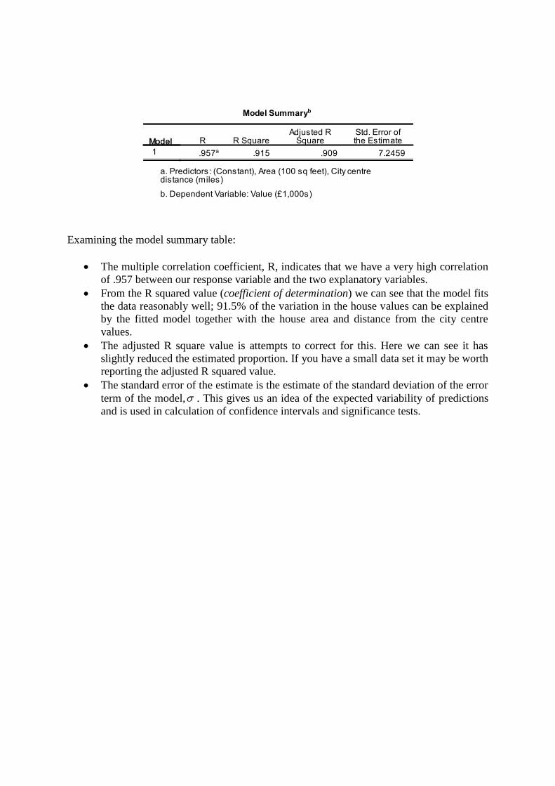
Examining the model summary table:

The multiple correlation coefficient, R, indicates that we have a very high correlation

of .957 between our response variable and the two explanatory variables.

From the R squared value (coefficient of determination) we can see that the model fits

the data reasonably well; 91.5% of the variation in the house values can be explained

by the fitted model together with the house area and distance from the city centre

values.

The adjusted R square value is attempts to correct for this. Here we can see it has

slightly reduced the estimated proportion. If you have a small data set it may be worth

reporting the adjusted R squared value.

The standard error of the estimate is the estimate of the standard deviation of the error

term of the model, . This gives us an idea of the expected variability of predictions

and is used in calculation of confidence intervals and significance tests.

The remaining output is concerned with checking the model assumptions of normality,

linearity and homoscedasticity of the residuals. Residuals are the differences between the

observed and predicted responses. The residual scatterplots allow you to check:

Normality: the residuals should be normally distributed about the predicted responses;

Linearity: the residuals should have a straight line relationship with the predicted

responses;

Homoscedasticity: the variance of the residuals about predicted responses should be

the same for all predicted responses.

The above table summarises the predicted values and residuals in unstandarised and

standardised forms. It is usual practice to consider standardised residuals due to their ease of

interpretation. For instance outliers (observations that do not appear to fit the model that well)

can be identified as those observations with standardised residual values above 3.3 (or less

than -3.3). From the above we can see that we do not appear to have any outliers.

The above plot is a check on normality; the histogram should appear normal; a fitted normal

distribution aids us in our consideration. Serious departures would suggest that normality

assumption is not met. Here we have a histogram that does look reasonably normal given that

we have only 30 data points and thus we have no real cause for concern.

The above plot is a check on normality; the plotted points should follow the straight line.

Serious departures would suggest that normality assumption is not met. Here we have no

major cause for concern.

The above scatterplot of standardised residuals against predicted values should be a random

pattern centred around the line of zero standard residual value. The points should have the

same dispersion about this line over the predicted value range. From the above we can see no

clear relationship between the residuals and the predicted values which is consistent with the

assumption of linearity.

Thus we are happy that the assumptions of the model have been met and thus would be

confident about any inference/predictions that we gain from the model.

Predictions

In order to get an expected house value for particular distance and area values we can use the

fitted equation. For example, for a house that is 5 miles from the city centre and is 1,400 ft2:

08.5132

14548.125456.9121.80

value

i.e. £208,513.

Alternatively, we could let a statistics program do the work and calculate confidence or

prediction intervals at the same time. For instance, when requesting a predicted value in SPSS

we can also obtain the following:

the predicted values for the various explanatory variable combinations together with

the associated standard errors of the predictions;

95% CI for the expected response;

95% CI for individual predicted responses.

Returning to our example we get the following:

the expected house value is £208,512 (s.e. = 2,067.6);

we are 95% certain that interval from £204,269 to £212,754 covers the unknown

expected house value;

we are 95% certain that interval from £193,051 to £223,972 covers the range of

predicted individual house value observations.