Multiple Regression

Multiple Regression

So far we have only examined the case where there is only one explanatory variable.

Often the variable we are interested in is related to more than one variable and their effects on Y

E.g.1 A firms share price may be a depend on the sales of the firm this year, the number of employees, where they sell their product etc….

E.g.2 House price depends on location, number of rooms, job opportunities in the region, population etc. etc.

Multiple Regression

The multiple regression model extends our analysis to more than one explanatory variable

Yi = β1X1i + β2X2i+ β3X3i +…+ βkXki + εi

Where X1t is a vector equal to unity [X1i=1] (i.e β1 is an

intercept) and XJi ( j= 2,3,…,k) is a set of explanatory variables

k = # of parameters to be estimated / degrees of freedom

Multiple Regression

Again we obtain fitted values

Again the aim is to minimise

Steps are same as before: Differentiate by each β and set each equal to 0 Solve the k first order conditions simultaneously to find the

β’s

n

iii

n

ii

YYMinMinkk

2

...,,

2

...,,

ˆ11

kikiiiiXXXXY ˆ...ˆˆˆˆ

332211

Interpretation of Coefficients in a Multiple regression Yi = β1X1i + β2X2i+ β3X3i +…+ βkXki + εi

Recall X1i here is just 1 so: Yi = β1 + β2X2i+ β3X3i +…+ βkXki + εi

Interpretation: Intercept (β1) -> Value of Y we would expect to observe if X2i,X3i,…,Xki

were ALL zero! Slopes:

β2 -> Change in Y we would expect to observe if X2 increased by one unit if all other X’s remained unchanged!!!

β3 -> Change in Y we would expect to observe if X3 increased by one unit if all other X’s remained unchanged!!!

βk -> Change in Y we would expect to observe if Xk increased by one unit if all other X’s remained unchanged!!!

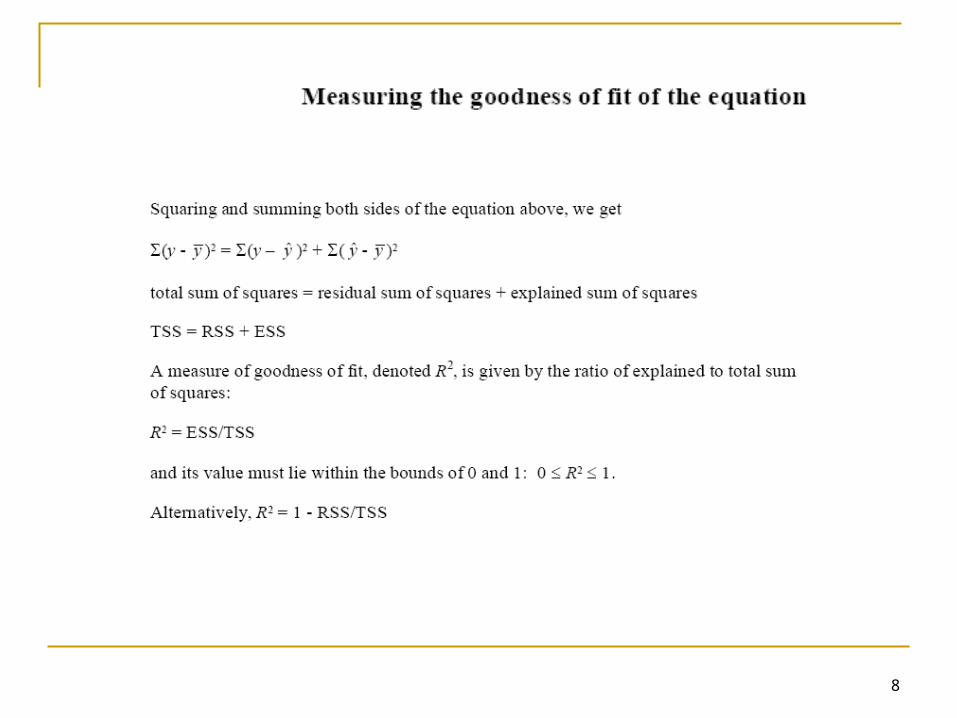
Goodness of Fit and Hypothesis Testing

We can decompose the deviation of Y from its mean value (Y) into a part explained by the fact that X is not at its average value, and a part which we cannot explain.

Naturally we would like to ‘explain’ as much of the variation in Y as possible.

7

X Xi

Y

Yi

=> This part is explained by variation in Xi from its mean

8

Goodness of Fit

We should be a little suspicious of models which appear to fit the data too well (e.g. r2 of 0.9 means we can explain 90% of the variation in Y using only X!)

9

R2 and adjusted R2

R2 measures the closeness of fit in the regression model Comparing two different regressions with different numbers

of explanatory variables causes difficulties Additional independent variables will always result in a higher

R2 regardless of their importance [because by chance they will appear to explain some variation]]

Instead, we use the adjusted R2 ( )

The model selection criterion is to include an extra explanatory variable only if it increases the adjusted R2

2R

)1/(

)/(1

2

nTSS

knRSSR

Other Model Selection Criterion (These are more commonly used than R2 in Time-series) Akaike Information Criterion (AIC)

Schwarz Bayesian Criterion (SBC)

Others include The Finite Prediction Error (FPE) Hannan and Quin Criterion (HQC)

nken

RSSAIC /2)(

nken

RSSSBC /)(

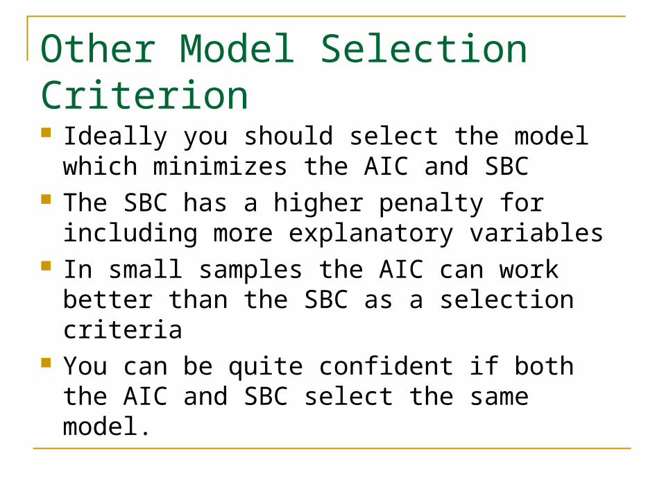
Other Model Selection Criterion Ideally you should select the model which

minimizes the AIC and SBC The SBC has a higher penalty for including

more explanatory variables In small samples the AIC can work better

than the SBC as a selection criteria You can be quite confident if both the AIC

and SBC select the same model.

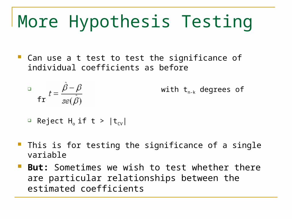
More Hypothesis Testing

Can use a t test to test the significance of individual coefficients as before

with tn-k degrees of freedom

Reject Ho if t > |tCV|

This is for testing the significance of a single variable But: Sometimes we wish to test whether there are

particular relationships between the estimated coefficients

Imposing Linear Restrictions Given the unrestricted equation

Yi = β1X1i + β2X2i+ β3X3i + β4X4i + β5X5i + εi

εi is a random shock with a mean 0

Impose the restriction β2 = β5

Our equation is then: Yi = β1 + β2X2i+ β3X3i + β4X4i + β2X5i + ei

Yi = β1 + β2(X2i+ X5i) + β3X3i + β4X4i + ei

Yi = β1 + β2(X*i) + β3X3i + β4X4i + ei

Where X*i = X2i+ X5i

Testing Linear Restrictions

Need to test whether your imposed restrictions are valid Key is to test the difference between the

unrestricted and restricted model If the restriction does not affect the fit of the model

very much then we can accept the restriction as being valid

How do we compare the restricted and unrestricted least-squares regressions?

Testing Linear Restrictions

The most common method is to estimate both the restricted and unrestricted equations and apply an F test The difference between RSSR and RSSU should be

minimal if the restrictions are valid

Where subscripts U and R stand for the unrestricted and restricted equations respectfully and k is the number of parameters in the model

)/(

)/()(

UU

RUUR

knRSS

kkRSSRSSF

Testing Linear Restrictions

Applying the Test1. H0 = Restrictions are valid

2. Estimate the restricted and unrestricted models. Calculate RSSR and RSSU

3. Calculate the F statistic

4. Find F critical for (kU – kr, n – ku) degrees of freedom form the F tables

5. If F- statistic > F critical reject H0

Testing the joint significance of all the explanatory variables

Yi = β1 + β2X2i+ β3X3i + β4X4i + β5X5i + ei

Test the restriction that β2= β3 = β4 = β5= 0 In other words, test the null hypothesis that none

of the coefficients in the model apart from the intercept are statistically significant

The F statistic is calculated automatically by most statistical packages for this test!

Adding or Deleting explanatory variables When only considering a single variable it is

safe to check its t-ratio When more than one variable is involved you

can apply the F test by estimating the restricted and unrestricted equations as discussed

Wald and LM Procedures

Wald and LM (Lagrange Multiplier) procedures are other ways of testing the validity of restrictions Wald procedure: By estimating the unrestricted

equation and applying a t-test to the restriction (e.g. the t-test on a single coefficient)

Lagrange Multiplier test: By estimating the restricted model only and then testing for a relaxation of the restrictions by applying a formula

These are both explained in Asteriou & Hall P74-75

Some other considerations

Type of Data used We will distinguish between 3 types of data:

Scale Data (e.g. X= 1,1.5, 2.7, 3.1 ,4.6 ,5,….) the numbers are measuring something, e.g. age, weight,

turnover, share price etc.

Ordinal Data: (e.g. X: 1= very good, 2= good, 3= ok, 4=bad 5= very bad). Numbers suggest some ordering but do not have a ‘true’ meaning Education example: if 1= primary, 2 = secondary 3= 3rd level A person with 3rd level education doesn’t have 3 times as much

education!!

Categorical data: Any numbers assigned here have no ‘real’ meaning Gender Example: 1= male 2= female. Can think of the numbers as just labels!!

Non-scale dependent variables (Y) Our Y variable (dependent variable) must be

a scale for the results of the models we use to have any (correct) meaning However if we are interested in non-scale

variables there are methods to deal with this – we won’t cover them – e.g. Probit if our model has just 2 categories etc.

If, in future work, you are unsure what sort of models to consider I can point you in (hopefully!) the right direction

Non-scale Explanatory variables (X’s) For ordinal variables:

The sign of the coefficient is reliable but the size of the coefficient is only likely to be reliable if the

levels are evenly spaced. (Often not the case, e.g. effect of moving from primary education

to secondary is not the same as moving from secondary to tertiary)

For categorical variables (e.g. County: 1=Dublin, 2= Wicklow, 3= ……) Often the sign has no meaning AND the size has no meaning

either However it is a common mistake for people starting out in

econometrics to mistakenly include these variables so be careful!!!

The correct Approach for dealing with categorical data (and for ordinal though less commonly used):

Dummy Variables

Dummy Variables

A dummy variable is a variable which takes a value of 1 for a certain group of observations and a 0 for all other observations. E.g. Male=1 Female=0

Adding a Dummy variable to our regression allows the groups to have different intercepts

Suppose we have data on Earnings and experience and we fit a regression: Yi = β1 + β2X2i + εi

Not using Dummy Variable

Seems to fit ok, but few of the observations lie very close to the line – seems to be a group above and a group below….

Y

X

Yi = β1 + β2X2i + εi

β1

Dummy variable for Gender Now suppose we also know gender: Create a dummy variable, D:

D=0 for females and D=1 for males Our regression is now:

Yi = β1 + β2X2i + β3D + εi

So: For Females: Yi = β1 + β2X2i + εi

For Males: Yi = β1 + β2X2i + β3 + εi

Rearranging this : Yi = (β1 + β3) + β2X2i + εi

We can see each group has a different intercept!!

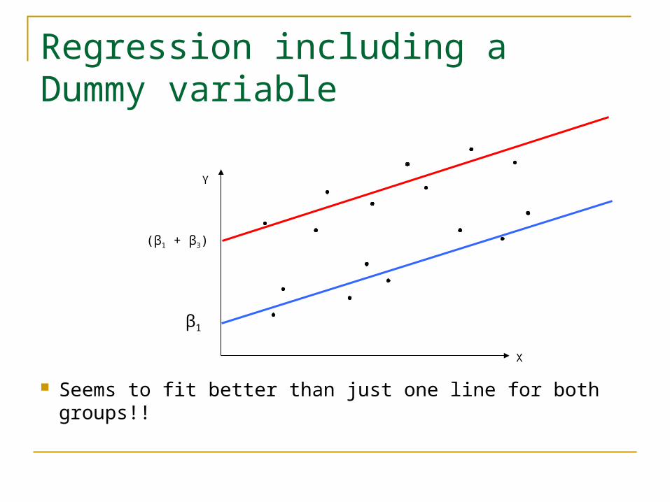
Regression including a Dummy variable

Seems to fit better than just one line for both groups!!

(β1 + β3)

Y

X

β1

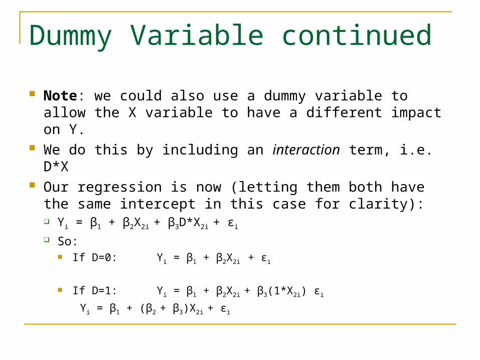
Dummy Variable continued

Note: we could also use a dummy variable to allow the X variable to have a different impact on Y.

We do this by including an interaction term, i.e. D*X Our regression is now (letting them both have the

same intercept in this case for clarity): Yi = β1 + β2X2i + β3D*X2i + εi

So: If D=0: Yi = β1 + β2X2i + εi

If D=1: Yi = β1 + β2X2i + β3(1*X2i) εi

Yi = β1 + (β2 + β3)X2i + εi

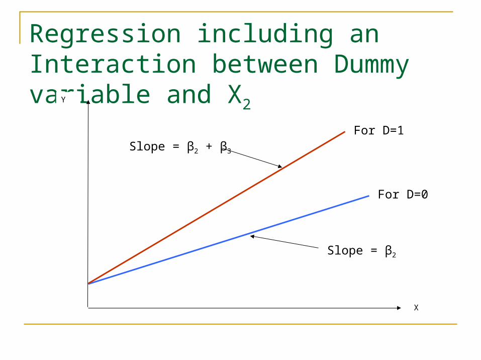
Regression including an Interaction between Dummy variable and X2Y

X

Slope = β2

Slope = β2 + β3

For D=1

For D=0

What if we think a variable doesn’t always have the same effect?

E.g. for wages, an extra year of experience may increase wages a lot, but after 20 years an extra year is unlikely to make much difference!!

Wages and Experience

We predict wages that are too high for low (and for high) experience but predict wages that are too low for medium experience workers

Wages

Experience

Yi = β1 + β2X2i + εi

β1

Fitting a curve

In algebra we would write the equation for a straight line as: Y=c + mX In econometric terms:

Yi = β1+ β2X1+ εi

In algebra the equation for a curve is: Y=c+ mX+nX2

So the equivalent in econometrics is:Yi = β1+ β2X1+ β3X2

1 +εi

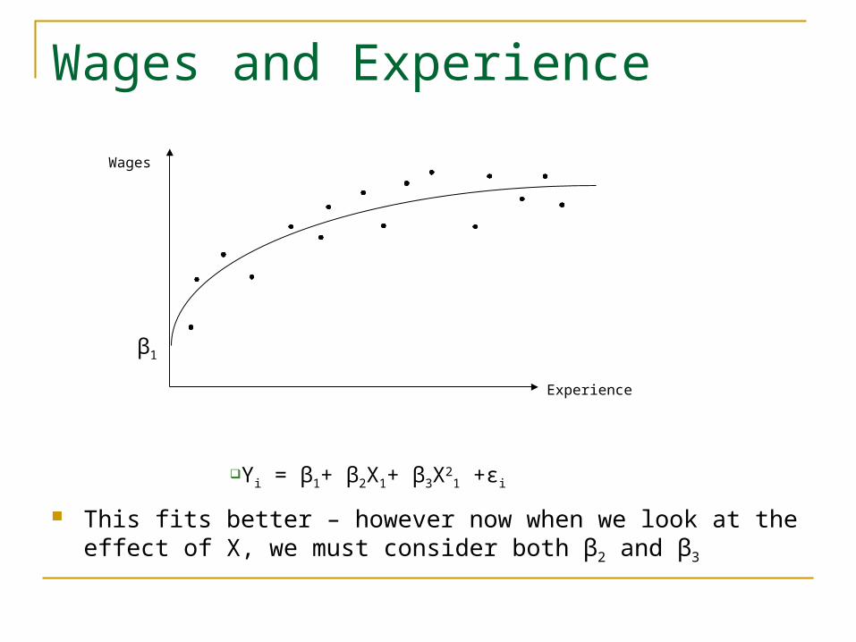
Wages and Experience

This fits better – however now when we look at the effect of X, we must consider both β2 and β3

Wages

Experience

Yi = β1+ β2X1+ β3X21 +εi

β1

Violations of Assumptions of OLS

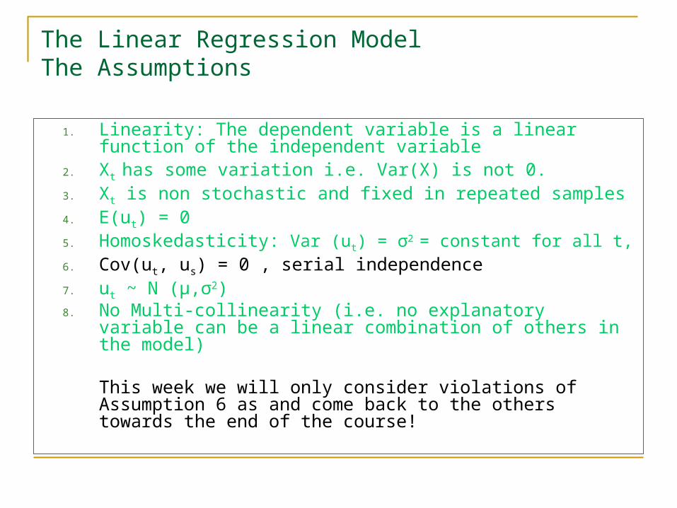
The Linear Regression ModelThe Assumptions

1. Linearity: The dependent variable is a linear function of the independent variable

2. Xt has some variation i.e. Var(X) is not 0.3. Xt is non stochastic and fixed in repeated samples4. E(ut) = 05. Homoskedasticity: Var (ut) = σ2

= constant for all t,

6. Cov(ut, us) = 0 , serial independence7. ut ~ N (μ,σ2)8. No Multi-collinearity (i.e. no explanatory variable can be a

linear combination of others in the model)

This week we will only consider violations of Assumption 6 as and come back to the others towards the end of the course!

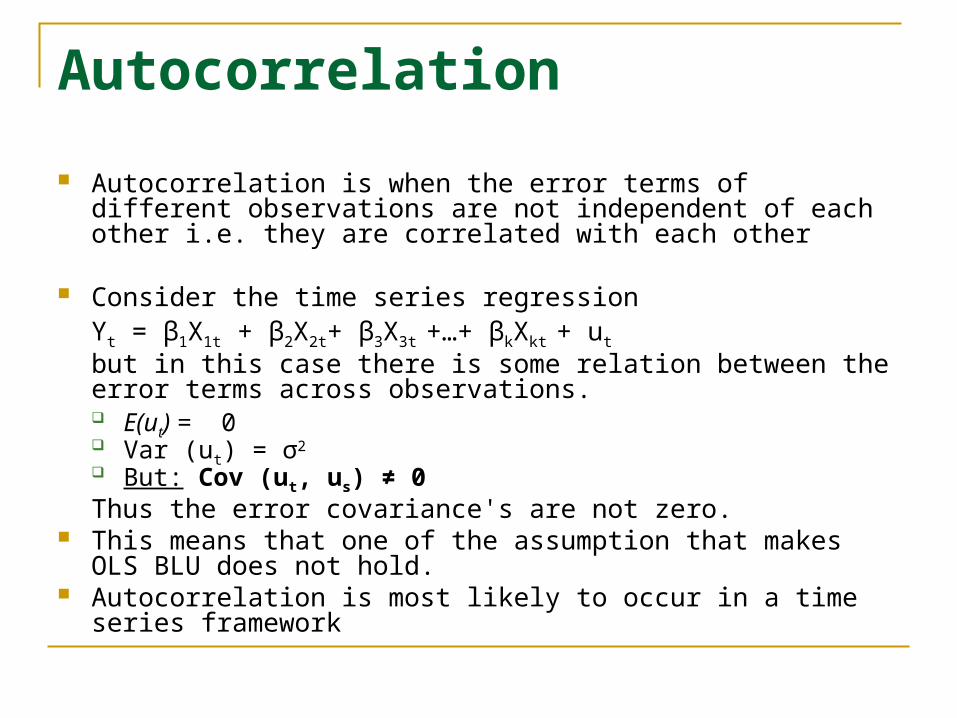
Autocorrelation

Autocorrelation is when the error terms of different observations are not independent of each other i.e. they are correlated with each other

Consider the time series regressionYt = β1X1t + β2X2t+ β3X3t +…+ βkXkt + ut

but in this case there is some relation between the error terms across observations. E(ut) = 0 Var (ut) = σ2

But: Cov (ut, us) ≠ 0Thus the error covariance's are not zero.

This means that one of the assumption that makes OLS BLU does not hold.

Autocorrelation is most likely to occur in a time series framework

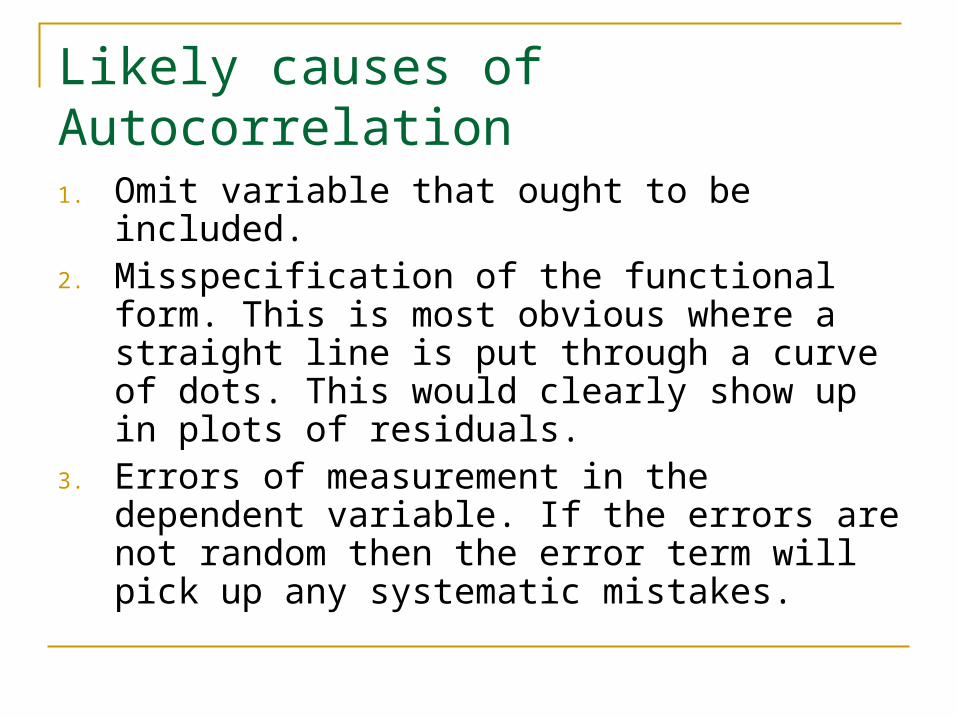
Likely causes of Autocorrelation

1. Omit variable that ought to be included.2. Misspecification of the functional form. This

is most obvious where a straight line is put through a curve of dots. This would clearly show up in plots of residuals.

3. Errors of measurement in the dependent variable. If the errors are not random then the error term will pick up any systematic mistakes.

The Problem with Autocorrelation OLS estimators will be inefficient and no

longer BLUE The estimated variances of the regression

coefficients will be biased and inconsistent, therefore hypothesis testing will no longer be valid. R2 will tend to be overestimated and t-statistics will tend to be higher

Autocorrelation Focus on simplest form of relation over time: first order

autocorrelation which can be written asut =ρut-1 + εt

Where │ρ│<1ρ is the parameter depicting the relationship among ut and ut-1. εt is a new error term.

The current observation of the error term is a function of the previous observation of the error term. First order serial correlation.

Higher order serial correlation can be modeled withut =ρut-1 + ρ2ut-2 + ρ3ut-3 +…+ ρkut-k + εt

Detecting Autocorrelation

By observation Plot the residuals against time Plot u^t against u^t-1

The Durbin Watson Test Only good for first order serial correlation It can give inconclusive results It is not applicable when a lagged dependent variable is

included in the regression Breusch and Godfrey (1978) developed an

alternative test

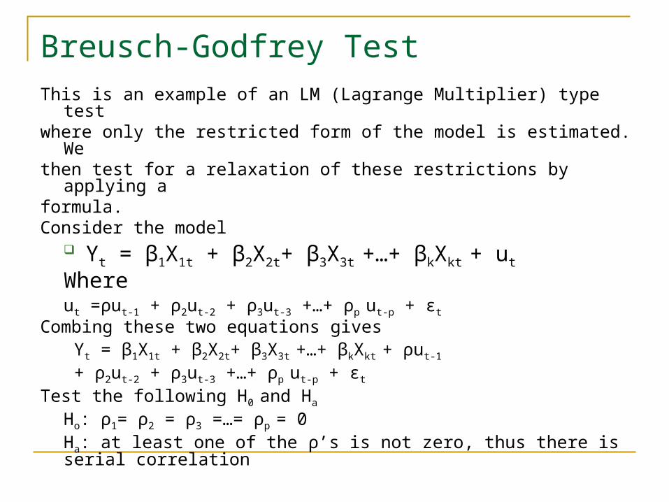
Breusch-Godfrey TestThis is an example of an LM (Lagrange Multiplier) type testwhere only the restricted form of the model is estimated. Wethen test for a relaxation of these restrictions by applying aformula.Consider the model

Yt = β1X1t + β2X2t+ β3X3t +…+ βkXkt + ut

Whereut =ρut-1 + ρ2ut-2 + ρ3ut-3 +…+ ρp ut-p + εt

Combing these two equations gives Yt = β1X1t + β2X2t+ β3X3t +…+ βkXkt + ρut-1

+ ρ2ut-2 + ρ3ut-3 +…+ ρp ut-p + εt

Test the following H0 and Ha

Ho: ρ1= ρ2 = ρ3 =…= ρp = 0Ha: at least one of the ρ’s is not zero, thus there is serial correlation

Breusch-Godfrey Test

This two-stage test begins be considering themodel

Yt = β1X1t + β2X2t+ β3X3t +…+ βkXkt + ut (1)

Estimate model 1 and save the residuals.Run the following model with the number of lagsUsed determined by the order of serial correlationyou are willing to test.

u^t = α0 + α1X2t+ α2X3t +…+ αRrXRt + αR+1 u^t-1 + αR+2u^t-

2 +…+ αR+p u^t-p

(auxiliary regression)

Breusch-Godfrey Test

The test statistic may be written as an LM statistic = (n - ρ)*R2,where R2 relates to this auxiliary regression.

The statistic is distributed asymptotically as chi-square

(χ2ρ) with ρ degrees of freedom.

If the LM statistic is bigger than the χ2ρ critical then we

reject the null hypothesis of no serial correlation andconclude that serial correlation exists

Ho: No Autocorrelation Here we have autocorrelation (Prob. F<0.05)

Also note previous residual is significant in regression

-30

-20

-10

0

10

20

30

-30 -20 -10 0 10 20 30

RESID

PR

EV

RE

SID

Solutions to Autocorrelation1. Find cause2. Increase number of observations3. Specify correctly4. E-views provides number of procedures eg Cochrane Orcutt -

last resort5. Most important: It is easy to confuse misspecified dynamics

with serial correlation in the errors. In fact it is best to always start from a general dynamic model and test the restrictions before applying the tests for serial correlation.

That’s all for today!

There are some questions on black board – you should try the five questions with a * beside them and e-mail your answers to me – No need to write too much - one page in total is fine (or less!)