Dissertation

zur Erlangung des Doktorgrades

Multiple Imputation for Complex Data

Sets

Daniel Salfrán Vaquero

Hamburg, 2018

Erstgutachter: Professor Dr. Martin Spieß

Zweitgutachter: Professor Dr. Matthias Burisch

Promotionsprüfungsausschuss (Tag der mündlichen Prüfung: 05.03.2018):

Vorsitzender: Prof. Dr. phil. Alexander Redlich

1. Dissertationsgutachter: Prof. Dr. Martin Spieß

2. Dissertationsgutachter: Prof. Dr. Matthias Burisch

1. Disputationsgutachter: Prof. Dr. Eva Bamberg

2. Disputationsgutachter: Prof. Dr. Bernhard Dahme

When you discover new information or a broader context you have to throw out the

old understanding, no matter how much sense it made to you. Getting it right in the

future is more important than the feeling of understanding you had in the past. – Dr.

Ben Tippet

Abstract

Data analysis, common to all empirical sciences, often requires complete data sets,

but real-world data collection will usually result in some values being not observed.

Many methods of compensation with varying degrees of complexity have been pro-

posed to perform statistical inference when the data set is incomplete, ranging from

simple ad hoc methods to approaches with refined mathematical foundation. Given

the variety of techniques, the question in practical research is which one to apply. This

dissertation serves to expand on a previous proposal of an imputation method based

on Generalized Additive Models for Location, Scale, and Shape. The first chapters of

the current contribution will present the basic definitions required to understand the

Multiple Imputation field. Then the work discusses the advances and modifications

made to the initial work on GAMLSS imputation. A quick guide to a software pack-

age that was published to make available the results is also included. An extensive

simulation study was designed and executed expanding the scope of the latest pub-

lished results concerning GAMLSS imputation. The simulation study incorporates a

comprehensive comparison of multiple imputation methods.

Contents

1 Introduction 1

1.1 State of the Art . . . . . . . . . . . . . . . . . . . . . . . . . . . . . . . . . . 2

1.2 Strengths and weaknesses of multiple imputation procedures . . . . . . 5

1.3 Research goals . . . . . . . . . . . . . . . . . . . . . . . . . . . . . . . . . . . 7

1.4 Outline of the dissertation . . . . . . . . . . . . . . . . . . . . . . . . . . . . 8

2 Statistical Inference with partially observed data sets 9

2.1 Why Multiple Imputation . . . . . . . . . . . . . . . . . . . . . . . . . . . . 9

2.2 Missing Data Mechanism . . . . . . . . . . . . . . . . . . . . . . . . . . . . 11

2.2.1 Missing Completely At Random (MCAR) . . . . . . . . . . . . . . 12

2.2.2 Missing at Random (MAR) . . . . . . . . . . . . . . . . . . . . . . . 12

2.2.3 Missing Not At Random (MNAR) . . . . . . . . . . . . . . . . . . . 15

2.2.4 Ignorability . . . . . . . . . . . . . . . . . . . . . . . . . . . . . . . . 15

2.3 Estimation of parameters with partially observed data . . . . . . . . . . 16

2.3.1 Incompletely observed response . . . . . . . . . . . . . . . . . . . 16

2.3.2 Incompletely observed covariates . . . . . . . . . . . . . . . . . . . 17

2.3.3 Discussion of assumptions . . . . . . . . . . . . . . . . . . . . . . . 17

3 Multiple Imputation 19

3.1 Combining rules . . . . . . . . . . . . . . . . . . . . . . . . . . . . . . . . . . 19

3.2 Validity of the MI estimator . . . . . . . . . . . . . . . . . . . . . . . . . . . 21

3.3 Frequentist Inference . . . . . . . . . . . . . . . . . . . . . . . . . . . . . . . 23

3.3.1 Finite Imputations . . . . . . . . . . . . . . . . . . . . . . . . . . . . 24

3.4 Number of Imputations . . . . . . . . . . . . . . . . . . . . . . . . . . . . . 26

3.5 Multivariate Missing Data . . . . . . . . . . . . . . . . . . . . . . . . . . . . 27

3.5.1 Joint Modeling . . . . . . . . . . . . . . . . . . . . . . . . . . . . . . 27

3.5.2 Fully Conditional Specification . . . . . . . . . . . . . . . . . . . . 28

3.5.3 Compatibility . . . . . . . . . . . . . . . . . . . . . . . . . . . . . . . 29

i

4 Imputation Methods 31

4.1 Bayesian Linear Regression . . . . . . . . . . . . . . . . . . . . . . . . . . . 31

4.2 Amelia . . . . . . . . . . . . . . . . . . . . . . . . . . . . . . . . . . . . . . . . 33

4.3 Hot Deck Imputation . . . . . . . . . . . . . . . . . . . . . . . . . . . . . . . 33

4.3.1 Predictive Mean Matching . . . . . . . . . . . . . . . . . . . . . . . 34

4.3.2 aregImpute . . . . . . . . . . . . . . . . . . . . . . . . . . . . . . . . 36

4.3.3 MIDAStouch . . . . . . . . . . . . . . . . . . . . . . . . . . . . . . . . 37

4.4 Iterative Robust Model-based Imputation . . . . . . . . . . . . . . . . . . 37

4.5 Recursive Partitioning . . . . . . . . . . . . . . . . . . . . . . . . . . . . . . 39

4.5.1 Classification and Regression Trees . . . . . . . . . . . . . . . . . . 39

4.5.2 Random Forest . . . . . . . . . . . . . . . . . . . . . . . . . . . . . . 40

5 Robust imputation with GAMLSS and mice 41

5.1 GAMLSS . . . . . . . . . . . . . . . . . . . . . . . . . . . . . . . . . . . . . . . 41

5.2 Imputation . . . . . . . . . . . . . . . . . . . . . . . . . . . . . . . . . . . . . 42

5.3 Software Implementation . . . . . . . . . . . . . . . . . . . . . . . . . . . . 45

5.4 Usage . . . . . . . . . . . . . . . . . . . . . . . . . . . . . . . . . . . . . . . . 47

5.5 Discussion . . . . . . . . . . . . . . . . . . . . . . . . . . . . . . . . . . . . . 49

6 Simulation Experiment 52

6.1 Experimental Design . . . . . . . . . . . . . . . . . . . . . . . . . . . . . . . 52

6.1.1 Single predictor . . . . . . . . . . . . . . . . . . . . . . . . . . . . . 54

6.1.2 Multivariate set . . . . . . . . . . . . . . . . . . . . . . . . . . . . . . 55

6.2 Single Predictor Results . . . . . . . . . . . . . . . . . . . . . . . . . . . . . 59

6.2.1 Normal . . . . . . . . . . . . . . . . . . . . . . . . . . . . . . . . . . . 60

6.2.2 Skew-Normal and Chi-squared distribution . . . . . . . . . . . . . 64

6.2.3 Uniform and Beta distribution . . . . . . . . . . . . . . . . . . . . . 68

6.2.4 Poisson . . . . . . . . . . . . . . . . . . . . . . . . . . . . . . . . . . . 72

6.2.5 Student’s t . . . . . . . . . . . . . . . . . . . . . . . . . . . . . . . . . 74

6.3 Multiple Incomplete Predictors . . . . . . . . . . . . . . . . . . . . . . . . . 76

6.3.1 Normal continuous predictor . . . . . . . . . . . . . . . . . . . . . 76

6.3.2 Non-Normal Predictors . . . . . . . . . . . . . . . . . . . . . . . . . 80

6.3.3 Weak MDM . . . . . . . . . . . . . . . . . . . . . . . . . . . . . . . . 83

6.3.4 Non-monotone MDM . . . . . . . . . . . . . . . . . . . . . . . . . . 85

7 Conclusion & Summary 87

7.1 Research Goals . . . . . . . . . . . . . . . . . . . . . . . . . . . . . . . . . . . 87

7.1.1 Relaxation of the assumptions of GAMLSS-based imputation mod-

els . . . . . . . . . . . . . . . . . . . . . . . . . . . . . . . . . . . . . . 87

ii

7.1.2 Imputation of multiple incompletely observed variables . . . . . 88

7.1.3 Comparison of the Imputation Methods . . . . . . . . . . . . . . . 89

7.2 Recommendations . . . . . . . . . . . . . . . . . . . . . . . . . . . . . . . . . 90

A R code for the example 92

B Extra Tables 94

iii

Chapter 1

Introduction

Missing data is a problem that exists within virtually any discipline that makes use of

empirical data. When performing longitudinal or cross-sectional studies in psycholog-

ical research, it is not uncommon for data to be missing either by chance or by design.

For instance, in research involving multiple waves of measurements, missing data can

arise due to attrition, that is, subjects drop out before the end of the study.

Typically, researchers have many standard complete-data techniques available, many

of which were developed early in the twentieth century like the ordinary least-squares

regression and factor analysis (Seal, 1967), when there was just no solution for han-

dling missing values. More modern techniques like the random effects model (Hen-

derson et al., 1959) or the logistic regression (Cox, 1958) that became accessible

before 1970 were also intended for complete data sets. Software packages like R,

SAS, and SPSS provide these routines. However, these methods, being complete-data

techniques, are not able of dealing correctly with incomplete data sets.

Simple solutions were in use for decades (Schafer and Graham, 2002). These

strategies involved discarding incomplete cases or substituting missing data by some-

how plausible values. The most popular approach is complete case analysis (CCA) also

known as listwise deletion. The method is simple, and no particular modifications are

needed. The main difficulty is that not all missing values have the same reason for

not being observed, and there are situations in which missing data do not affect the

conclusions, but generally, no justification is provided for the assumptions underlying

the analysis at hand.

Neglecting the missing data problem can result in adverse consequences such as

the loss of statistical power of a given analysis due to the reduction of the sample size,

or even worse, missing values may invalidate the conclusions for the data and lead to

wrong statistical inference. Today, disadvantages of these methods are well known in

both the statistical and applied literature (Little and Rubin, 2002).

1

1.1 State of the Art

There are two primary schools about how to deal with the missing data problem.

On one side, there are model-based methods mainly built around the formulation of

the Expectation-Maximization (EM) algorithm made popular by Dempster, Laird, and

Rubin (1977). This technique makes the computation of Maximum Likelihood (ML)

estimator feasible in problems affected by missing data. In short, the EM algorithm

is an iterative procedure that produces maximum likelihood estimates. The idea is

to treat the missing data as random variables to be removed by integration from the

log-likelihood function as if they were not sampled. The EM algorithm allows dealing

with the missing data and parameter estimation in the same step. The major draw-

back of this model-based method is the requirement of the explicit modeling of joint

multivariate distributions and, thus, tend to be limited to variables deemed to be of

substantive relevance (Graham, Cumsille, and Elek-Fisk, 2003). Furthermore, this

approach requires the correct specification of usually high-dimensional distributions,

even of aspects which have never been the focus of empirical research and for which

justification is hardly available. According to Graham (2009), the parameter estima-

tors (means, variances, and covariances) from the EM algorithm are preferable over a

wide range of possible estimators, based on the fact that they enjoy the properties of

maximum likelihood estimation.

The second approach deals with model-based missing data procedures and was

introduced by Rubin (1987) with his concept of Multiple Imputation (MI). Instead of

removing the missing values by integration as EM does, MI simulates a sample of m

values from the posterior predictive distribution of the missing values given the ob-

served. Each missing value is replaced by this approach with m > 1 possible values,

accounting for uncertainty in the values predicting the true but unobserved values.

The substituted values are called “imputed” values, hence the term “Multiple Imputa-

tion.”

MI can be summarized in three steps. The first step is to create m sets of completed

data by replacing each missing value with m imputed values. The second phase con-

sists of using standard statistical methods for separate analysis of each completed data

set as if it were a “real” completely observed data set. The third step is the pooling

step where the results from m analyses are combined to form the final results and al-

lows statistical inference in the usual way. This technique has become one of the most

advocated methods for handling missing data.

The MI framework comprises three models: The complete data model, the nonre-

sponse model, and the imputation model. The complete data model is the one used

to make inferences of scientific interest. For example, a linear regression including

2

the outcome and explanatory variables of an experiment. The nonresponse model

represents the process that leads to missing data. The covariates in the nonresponse

model are not primarily of interest, and they are not necessarily part of the complete

data model. The imputation model is the model from which plausible values for each

missing datum are generated. A problematic step of MI procedures is the specifica-

tion of the imputation model because the validity of the analysis of the complete data

model strongly depends on how imputations are created. If the imputation model is

not correctly specified, then final inferences may be invalid.

There are two ways of specifying imputation models: Joint modeling (JM) and

fully conditional specification (FCS). Joint modeling involves specifying a multivari-

ate distribution for the variables whose values have not been observed conditional

on the observed data and then drawing imputations from this conditional distribu-

tion by Markov chain Monte Carlo (MCMC) techniques (Schafer, 1997). On the other

hand, with the fully conditional specification, also known as multivariate imputation

by chained equations (van Buuren and Groothuis-Oudshoorn, 2011), a univariate im-

putation model is specified for each variable with missings conditional on other vari-

ables of the data set. Initial missing values are imputed with a bootstrap sample, and

then subsequent imputations are drawn by iterating over conditional densities (van

Buuren, 2007; van Buuren and Groothuis-Oudshoorn, 2011).

Within the JM framework, Little and Rubin (2002), Rubin (1987), and Schafer

(1997) have developed imputation procedures for multivariate continuous, categor-

ical and mixed continuous and categorical data based on the multivariate normal,

log-linear and general location model, respectively. There has also been development

in univariate models for modeling semicontinuous data. Javaras and Dyk (2003) in-

troduced the blocked general location model (BGLoM), designed for imputing semi-

continuous variables with the help of EM and data augmentation algorithms.

Another device that can be used to generate imputations is nonparametric tech-

niques, like hot deck methods. Based on hot deck methods, the missing values are

imputed by finding a similar but observed unit, whose value serves as a donor for the

record of the similar but incompletely observed unit. The most popular are k-nearest-

neighbor algorithms from which the best known method for generating hot-deck impu-

tations is the Predictive Mean Matching (PMM) (Little, 1988), which imputes missing

values employing the nearest-neighbor donor distance base on expected values of the

missing variables conditional on observed covariates. There are several advantages

of kNN imputation. It is a simple method that seems to avoid strong parametric as-

sumptions, it can easily be applied to various types of variables to be imputed, and

only available and observed values are imputed (e.g., Andridge and Little, 2010; Lit-

tle, 1988; Schenker and Taylor, 1996). However, the final goal of the complete data

3

statistical analysis is to make inferences about the population represented by the sam-

ple; therefore, the plausibility of imputed values is not the defining factor in choosing

an imputation model over another. Instead, the proper criterion is the validity of the

final analysis of scientific interest.

Recent research on improving the performance of kNN methods focused on the dis-

tance function and the donor selection. Tutz and Ramzan (2014) proposed a weighted

nearest neighbor method based on Lq-distances and Siddique and Belin (2008) and

Siddique and Harel (2009) propose a multiple imputation method using a distance-

aided selection of donors (MIDAS). The latter technique was extended and imple-

mented in R by Gaffert, Meinfelder, and Bosch (2016). Harrell (2015) proposed the

aregImpute algorithm which combines aspects of model-based imputation methods in

the form of flexible nonparametric models with the predictive mean matching.

Modern methods like Amelia (Honaker, King, and Blackwell, 2011) or irmi (Templ,

Kowarik, and Filzmoser, 2011) and even hot deck methods like PMM (Little, 1988)

make use of linear imputation models explicitly or implicitly. However, the condi-

tional normality of the dependent variable in a homoscedastic linear model with in-

completely observed metric predictors alone is not sufficient to justify a linear imputa-

tion model for the incompletely observed variable. Thus, assumed linear imputation

models would not, in general, be compatible with the true data generating process.

Although it has been proposed to transform variables to assume multivariate normal-

ity more plausible (e.g., Honaker, King, and Blackwell, 2011; Schafer, 1997), this

technique does not work in general (e.g., Hippel, 2013). The distribution of variables

in the observed part of the data set might be very different from the distribution of

the same variables if there were no missing values. In an experiment, Hippel (2013),

showed that transformed imputation models led to biases in the estimators.

A newly proposed method by de Jong (2012) and de Jong, van Buuren, and

Spiess (2016) makes use of Generalized Additive Models for Location Scale, and Shape

(GAMLSS). The proposed method fits a nonparametric regression model with spline

functions as a way of specifying the individual conditional distribution of the vari-

ables with missing values which can be used in the framework of chained equations.

Roughly, the idea is to use semi-parametric additive models based on the penalized

log-likelihood and then fit the conditional parameters for location, scale, and shape

using a smoother. In principle, the specification of the conditional distribution can

be arbitrary, though de Jong, van Buuren, and Spiess (2016) mainly used the normal

distribution.

4

1.2 Strengths and weaknesses of multiple imputation

procedures

An important notion concerning the success of the method of multiple imputation is

the hypothesis of “proper” multiple imputation. The concept of proper imputations

is based on a set of conditions imposed on the imputation procedure. An imputation

method tends to be proper if the imputations are independent draws from an appropri-

ate posterior predictive distribution of the variables with missing values given all other

variables (Rubin, 1987). This implies, that both, the average of the m point estimators

is a consistent, asymptotically normal estimator of the parameter of scientific interest

and that an estimator of its asymptotic variance is given by a combination of the within

and between variance of the point estimators. Meng (1994) showed the consistency

of the multiple imputation variance estimator as the number of imputations tends to

infinity but restricted his analysis to “congenial” situations, in which imputation and

analysis models match each other in a certain sense. In contrast, Nielsen (2003) claims

that MI “is inefficient even when it is proper.”

According to Rubin (1996), there are two distinct points of interest about multiple

imputation. The first type focus on its implementation: operational difficulties for

the imputer and the ultimate user, as well as the acceptability of answers obtained

partially through the use of simulations. The second type concerns the frequentist

validity of repeated-imputation inferences when the multiple imputation is not proper

but seems “reasonable” in some sense. Rubin (1996) states that statistical validity,

according to the frequentist definition, is difficult because it requires both that the

imputation model with the assumptions considered by the imputer are correct and

the complete-data analysis would have been already valid if there were to missing

values (“Achievable Supplemental Objective”, Rubin, 1996).

Rubin (2003) acknowledged that there are reasons for concerns about the meth-

ods since it is not yet proven in a strict mathematical sense that the multiple impu-

tation method allows valid inferences in all situations of interest. Many statements

are based on heuristics and simulation results, and there is almost always some un-

certainty in choosing the correct imputation model. On the other hand, according

to Rubin (2003), multiply-imputed data analyses using a reasonable but imperfect

model can be expected to lead to slightly conservative inferences, that is, inferences

that have coverage that is slightly larger than the nominal (1− α) percent. Theoret-

ical arguments, as well as some empirical results based on simulations, imply that

standard multiple imputation techniques may be rather robust concerning slight mis-

specifications of the imputation model, probably leading to larger confidence intervals

and overestimation of variances. This is called the “self-correcting” property of mul-

5

tiple imputation methods (e.g., Little and Rubin, 2002; Rubin, 1996, 2003). Robins

and Wang (2000) question the validity of the variance estimator proposed by Rubin

(1987) and claim that in large samples the MI variance estimator may be downward

biased.

Most results about individual imputation methods rely on simulated experiments.

Schafer (1997) and Schafer and Graham (2002) argue that simulations or artificial

experiments are a helpful instrument to investigate the properties of MI-based infer-

ences since, by definition, these methods are based on random draws from a posterior

distribution, akin to the application of Markov chain Monte Carlo routines. There

are many examples of recent studies that based their results on simulations. Deng

et al. (2016) developed an imputation method based on regularized regressions that

presented a small bias but acceptable coverage rates in a simulation experiment. Don-

neau et al. (2015a,b) ran two comparison studies of multiple imputation methods for

monotone and non-monotone missings patterns in ordinal data which found that nor-

mal assumptions for MI resulted in biased results. Kropko et al. (2014) compared the

JM and FCS imputation approaches for continuous and categorical data, reporting

better results for FCS.

He and Raghunathan (2009) evaluated the performance and sensitivity of sev-

eral imputation methods to deviations from their distributional assumptions. They

found that, concerning the estimation of regression coefficients, currently used mul-

tiple imputation procedures can, in fact, give worse performance than complete case

analyses that ignore the missing mechanism about bias and variance estimation under

seemingly harmless deviations from standard simulation conditions. Yu, Burton, and

Rivero-Arias (2007) and then Vink et al. (2014) appraised the performance of multiple

imputation software on semicontinuous data with mixed results showing that depar-

tures from linear or normality assumptions yielded worse estimates in general. They

concluded that the most reliable methods were based on PMM, but de Jong (2012)

and de Jong, van Buuren, and Spiess (2016) show that this is not necessarily true.

They find that PMM can systematically underestimate the standard errors, leading to

invalid inferences. To sum up, it is not yet known which imputation technique is most

appropriate in which situation, and which is flexible and robust enough to work in a

broad range of possible applications. One goal of the current work is to enhance the

GAMLSS imputation method and perform extensive simulation experiments under a

broad spectrum of experimental and practically relevant conditions.

6

1.3 Research goals

The GAMLSS approach defined in de Jong, van Buuren, and Spiess (2016) models

additively individual location parameters like the conditional means of the variables to

be imputed based on spline functions, which allows more flexibility than with standard

imputation methods. An error term randomly selected from a normal distribution is

added to generate imputations.

Simulation results in de Jong (2012) and de Jong, van Buuren, and Spiess (2016)

imply that inferences tend to be valid adopting this imputation technique, even if

the real underlying distribution of the covariables is Poisson or Chi-square. De Jong

(2012) concluded that if the variable with missings is heavy-tailed like a Student’s t,

the imputation method may not be proper anymore, leading to severely underesti-

mated variances of the estimators of scientific interest. Posterior analyses show that

the same could happen with a missing mechanism thinning out specific regions in the

data set.

A solution to this problem could be to replace the normal model for the error term

with a more general family of distributions like the four-parameter Johnson SU family

that in addition to the mean and variance also accounts for skewness and kurtosis of

the actual error distribution.

Objective 1: Therefore, the first objective of this work is to relax the distributional

assumption of the error within the GAMLSS imputation method to distributions with

unknown mean, variance, skewness, and kurtosis.

A limiting feature of the simulation results in previous works for the GAMLSS im-

putation method is that the method was mostly tested in bivariate data sets and only

one multivariate experiment where the variables were all independent and normally

distributed. Also, there was always only one variable incompletely observed. Real-

world applications require robust methods capable of dealing with complex data sets,

where the variables are not independent of each other and interactions exist.

Objective 2: Thus, the second objective is to extend the GAMLSS-based imputa-

tion methods to the multivariate case and evaluate them concerning the validity of

parameter estimators of scientific interest.

For the developed methods and algorithms to be helpful, it is necessary to show

that they allow valid inference when used in applications. Analyzing the large-sample

properties of the new method in an MI scenario proves to be very difficult. However,

the growing use of computational statistics allows the use of Monte Carlo simulation

as an alternative way to analyze the properties of the proposed method.

Objective 3: The final objective is to perform extensive empirical comparisons of

the two GAMLSS approaches with available modern techniques via simulation exper-

7

iments to allow justified guidance in applied in empirical sciences.

This is an important point in current research since if a self-correcting property of

MI holds, misspecification of imputation models would have only a minor effect on

the validity of inferences with increasing sample sizes and therefore is of interest to

test such relationship.

1.4 Outline of the dissertation

The first two chapters of the dissertation discuss the basic theoretical inferential as-

pects of the missing data problem. Chapter 2 introduces the model of scientific in-

terest and taxonomy of the missing data mechanisms. The ignorability of the missing

mechanism and the validity of complete-data procedures are also discussed. Chapter

3 focuses on the validity of Rubin’s MI estimators and the steps required to perform

standard statistical inference. Some topics like the number of imputations and the

available methods for multivariate data sets are also discussed.

Chapter 4 describes some of the most used imputation methods imputation meth-

ods. Chapter 5 presents the GAMLSS-based imputation method. The experimental

design and results of the comparison will be discussed in Chapter 6.

8

Chapter 2

Statistical Inference with partially

observed data sets

Real-world data sets often are only partially observed. This chapter discuss aspects

of the statistical inference and general concepts related to the missing data problem.

Section 2.1 presents the model of scientific interest, and discusses how to address the

consistent and valid estimation of its parameters. Most importantly, the section intro-

duces the concepts of Complete Case Analysis and Multiple Imputation, and defines

the notation to be used in the manuscript. Section 2.2 formalizes a classification of the

Missing Data Mechanisms (MDM). Section 2.3 discusses the effect of assumptions of

the missing data mechanism when estimating the parameters in a regression model.

2.1 Why Multiple Imputation

Let’s suppose that given Y = (Yi j), i = 1, . . . , n and j = 1, . . . , p, a matrix with the

observations for n units on p variables we want to make inferences about the vector

of population parameters θ T = (θ1, . . . ,θp). We define the model

E[U(Yi,θ )] = 0, (2.1)

where U is a (p × 1) real-valued function. This is actually a just-identified General-

ized Method of Moments (GMM) model and with different choices of U , encompasses

many common used applications like linear and nonlinear regression models, maxi-

mum likelihood estimation or instrumental variable regression (Cameron and Trivedi,

2005, Chapter 6).

The objective of statistical research is to provide valid inference about θ . Assuming

that the data is fully observed, Cameron and Trivedi (2005) show that consistent and

9

valid estimators bθ and bΣ for the model in equation (2.1) can be obtained as:

bθ = argminθ

1n

n∑

i

U(Yi,θ )

T

1n

n∑

i

U(Yi,θ )

, (2.2)

bΣ=

∂∑n

i U(Yi,θ )

∂ θ

−1 n∑

i

n∑

i′U(Yi,θ )U(Yi′ ,θ )

T

∂∑n

i U(Yi,θ )

∂ θ

T−1

. (2.3)

Let’s suppose that the data Y is only partially observed. The observed and miss-

ing parts of variable Yj are denoted by Y obsj and Y mis

j , respectively. Let’s define the

missing indicator, R, as binary matrix representing the missing data pattern. For each

individual unit i and variable j, let Ri j = 1 if Yi j is observed and Ri j = 0 if Yi j is missing.

One naive approach to still perform the statistical analysis in the presence of miss-

ing values is to use complete case analysis (CCA). This method would delete all units

with missing values, i.e., remove unit Yi if ∃ j : Ri j = 0. The estimators bθ and bΣ would

still be obtained through equations (2.2) and (2.3) replacing Y by the reduced, but

fully observed, data set Y obs. Whether CCA keeps consistency and validity of the es-

timators is a different matter. The answer to that problem depends on the specific

statistical analysis and the underlying mechanism that led to some values not being

observed. Example of this are discussed in section 2.3.

Using the Law of Iterated Expectations in model (2.1), a consistent estimator of

θ without ignoring incompletely observed data, as with CCA, can be obtained from

solving:

E f (Y mis|Y obs ,R)

U(Y obs, Y mis,θ )

= 0. (2.4)

where (Y obs, Y mis) is a partition of the data set into its observed and missing parts and

f (Y mis|Y obs, R) is the conditional predictive distribution of the missing data. If U(·)is the score function, a consistent estimator of the covariance matrix of θ using the

Fisher-information matrix. This can be obtained with Louis’s formula (Louis, 1982):

I (θ ) = Eθ

∂ U(Y,θ )θ

− E f (Y mis|Y obs ,R)[U(Y,θ )U(Y,θ )T ]

+ E f (Y mis|Y obs ,R)[U(Y,θ )]E f (Y mis|Y obs ,R)[U(Y,θ )]T (2.5)

The actual usefulness of equations (2.4) and (2.5) in specific applications differs

notably. Even for standard regression problems with incomplete data there are no gen-

eral solution methods and unique solutions have to be developed, often quite complex

and of limited use. For example, Elashoff and Ryan (2004) propose a solution based

on the EM algorithm that require the specification of additional moment conditions

10

to characterize the conditional expectations of the missing data. Approaches like this

become quickly unmanageable as the models get more complex than a standard re-

gression (Carpenter and Kenward, 2012).

Multiple Imputation (Rubin, 1987) will provide an indirect way to solve the esti-

mation problem. The key idea behind it is to reverse the order of the expectation and

estimation in equation (2.4). The essence is to repeat the following steps:

1. draw eY mis from f (Y mis|Y obs, R),

2. solve E

U(Y obs, Y mis,θ )

= 0.

and combine the results somehow to perform the inference. This provides an alterna-

tive to complex methods, allowing the use of the “complete data” methods given by

equations (2.2) and (2.3) in the estimation step. The eY mis imputed values are draws

from the Bayesian conditional predictive distribution of the missing observations. The

model, f , used to produce the imputations is called the “imputation model”. One of

the advantages of the MI method is that the model of scientific interest and the impu-

tation model can be fitted separately. The combination rules and the justification of

this method is discussed in chapter 3.

2.2 Missing Data Mechanism

The performance of missing data techniques strongly depends on the mechanism that

generated the missing values. Standard methods for handling missing values usually

make implicit assumptions about the nature of these causes. The missing data mech-

anism can be defined as

P(Ri|Yi,ψ), (2.6)

which is the probability of observing the values of Yi given their actual data and a vec-

tor of parameters, ψ, of the underlying missing mechanism. An implicit assumption

being made is that the values of Yi j exist regardless of whether they are observed or

not.

The focus of the model of scientific interest in section 2.1 is estimation of θ . The

parameterψ of the missing mechanism in equation (2.6) has no innate scientific value

and therefore it makes sense to ask if and when its estimation could be safely ignored.

Rubin (1976, 1987) formalized a system of missing mechanisms that classify missing

data problems in three categories: missing data either being missing completely at

random (MCAR), missing at random (MAR) or missing not at random (MNAR).

To exemplify the different classes, let’s consider an hypothetical clinical trial on the

effects of a given drug for the treatment of depression. In this study 200 patients with

11

depression are randomly assigned to one of two groups, one with an experimental drug

and the other with a placebo. Participants completed a depression scale, e.g., HAMD

(Hamilton, 1964) or BDI (Beck et al., 1996) after the end of treatment. Let Y1 take on

values 0 and 1 if participants were in the placebo or treatment group respectively, and

Y2 be the depression scores after the treatment. Some of the values of Y2 are missing

according to the following mechanism

P(Ri2 = 0) =ψ0 + [0.3Yi1 + 0.9(1− Yi1)]ψ1 +

1−Yi2

8+ Yi2

ψ2, (2.7)

which is just an example that based on the values of ψ0, ψ1, and ψ2 will help to

illustrate the different types of missing mechanism.

2.2.1 Missing Completely At Random (MCAR)

Missing data is said to be MCAR if the probability of the observed pattern of observed

and missing data does not depend on any of the other variables relevant to the analysis

of scientific interest, observed or not. Mathematically this can be expressed as,

P(Ri|Yi,ψ) = P(Ri|ψ). (2.8)

The MCAR mechanism exemplifies an event where missing values happen entirely

by chance, and it is a rather strong assumption.

Suppose that, in the example, we wish to estimate the mean depression rating

at the end of the study given the treatment group. The participants flipped a coin,

and based on the outcome decided whether to fill out the questionnaire at the end of

the study. The same can be expressed with equation (2.7) by setting ψ = (0.5, 0,0)leading to

P(Ri2 = 0) = 0.5.

In this scenario the missing values are MCAR and since the probability of not being

observed is unrelated to the values of Y1 or Y2, the observed part of the data is non-

selective with respect to the population. Valid inferences can be obtained from the

observed values.

2.2.2 Missing at Random (MAR)

The missing mechanism is MAR if the probability does depend on observed values of

the relevant variables but not additionally on relevant unobserved values of variables.

If Yi is partitioned as (Y obsi , Y mis

i ), representing the observed and unobserved parts of

12

Yi, then

P(Ri|Yi,ψ) = P(Ri|Y obsi ,ψ). (2.9)

The MAR mechanism is considerably weaker than the MCAR. Equation (2.9) doesn’t

imply that the probability of observing a variable is independent of its value. What

the MAR assumption means is that conditional on the observed data, the probability

of observing a variable doesn’t depends on its value.

observed mean: 8.96observed mean: 14.47

94/100 observed

33/100 observed

0

5

10

15

20

25

30

placebo drug

HA

MD

rat

ing

missingobserved

Figure 2.1: Plot of hypothetical depression rating scale values against treatment group

Let’s continue with the depression rating example. Figure 2.1 shows a scenario

where ψ= (0,1, 0) in equation (2.7), leading to the missing mechanism

P(Ri2 = 0) = 0.3Yi1 + 0.9(1− Yi1), (2.10)

meaning that participants in the placebo group are less likely to complete the ques-

tionnaire at the end of the study as compared with participants in the drug group, that

is, given the value of Yi1, the probability of missing Yi2 is either 0.9 or 0.3 independent

of its value conditional on the treatment group. This means that the missing scores

at the end of the study are MAR conditional on the treatment group. A consequence

of this missing data mechanism is that the estimation of the marginal mean will be

13

downward biased. A hypothetical data set was simulated with arbitrary mean depres-

sion scores of 9 and 15.5 for the drug and placebo groups respectively, so that the true

marginal mean is 12.25. However, the observed mean is

(94× 8.96+ 33× 14.47)/127= 10.39. (2.11)

based on the values recorded in Figure 2.1.

Due to the missing depression scores being MAR conditional on the treatment

group, it can be shown that the distribution of unobserved and observed ratings is

the same within each treatment group. Mathematically,

P(Yi2|Yi1,ψ, Ri2 = 0) =P(Yi1, Yi2,ψ, Ri2 = 0)

P(Yi1,ψ, Ri2 = 0)

=P(Ri2 = 0|Yi1, Yi2,ψ)P(Yi1, Yi2,ψ)

P(Ri2 = 0|Yi1,ψ)P(Yi1,ψ)

= P(Yi2|Yi1,ψ), (2.12)

using the fact that missing depression scores are MAR conditional on treatment group

in the last equality, since

P(Ri2 = 0|Yi1, Yi2,ψ) = P(Ri2 = 0|Yi1,ψ). (2.13)

The same claim is valid for Ri2 = 1, so the distribution of depression scores given

treatment group is the same in the observed and unobserved data, and the population.

The argument presented is akin to say that within treatment groups, depression

rating is MCAR. We can use that fact to estimate the marginal mean, scaling up the

averages of the mean in each group to yield a better estimate,

(100× 8.96+ 100× 14.47)/200= 11.71. (2.14)

This is equivalent to replace the missing values in each of the treatment groups by the

mean of the group.

Two further points need to be made. First, under the MAR assumption, the exact

details of the missing mechanism, such as the ψ parameter, don’t have to be specified

(Carpenter and Kenward, 2012). Second, it’s important to notice that the assump-

tion of the depression score being MAR (or MCAR) given the treatment group is an

untestable claim. The data needed to test is, of course, missing.

14

2.2.3 Missing Not At Random (MNAR)

Finally, the unobserved data is MNAR if the probability of the pattern of observed

and missing data does depend not only on observed but also on unobserved values of

variables relevant to the research question, that is,

P(Ri|Yi,ψ) 6= P(Ri|Y obsi ,ψ). (2.15)

If in our depression study example, we let ψ = (0, 0,1), the missing mechanism

(2.7) turns into

P(Ri2 = 0) = 1−Yi2

8+ Yi2

which means that participants with higher values of depression scores, or side-effects

from the experimental drug are more likely not to be present at the end of the study.

Then the probability of observing a value it is dependent on the value itself, like in the

missing mechanism shown, where the response indicator of Y2 depends on Y2. This

defines a MNAR mechanism.

Although it seems like the MNAR assumption could be more likely in real-world ap-

plications than MAR, statistical analyses are far more difficult. Under MAR, equation

(2.13) shows that the conditional distribution of partially observed variables coincide

for units with observed and unobserved values. This is not true under MNAR.

2.2.4 Ignorability

The classification system of Rubin (1976) define conditions under which θ can be

accurately estimated without being affected by ignoring ψ. According to Little and

Rubin (2002, Section 5.3), the missing data mechanism is ignorable if the missing

data are at least MAR and the joint parameter space (θ ,ψ) is the product of the pa-

rameter spaces of θ and ψ, that is, θ and ψ are distinct. Since the model of scientific

interest is not the missing data mechanism itself and usually knowing θ will add little

information aboutψ and the other way around according to Schafer (1997), the MAR

requirement is considered the most important condition (van Buuren, 2012).

More precisely, a valid analysis can be constructed without the necessity of ex-

plicitly including the model for the missing data mechanism. In the context of this

analysis, the missing mechanism can be ignored when applying the method of impu-

tation to compensate for missing data.

A consequence of the concept of ignorability is represented by equation (2.12)

which implies that

P(Y mis|Y obs, R= 1) = P(Y mis|Y obs, R= 0).

15

Hence, if the missing data mechanism is ignorable, the conditional predictive distri-

bution in equation (2.4), f (Y mis|Y obs, R) can be modeled with just the observed data.

On the other hand, if missing data are MNAR, then the missing mechanism can

not be ignored, and strong assumptions or external knowledge is usually necessary to

compensate for the missing data. The focus of the current research will be on ignorable

missing mechanisms.

2.3 Estimation of parameters with partially observed

data

It is of importance to analyze the connotations of the missing data mechanism for the

estimation of θ , the parameter in the scientific model of interest. The argument about

ignorability ofψ, the parameter of the MDM, does not imply a one-to-one relationship

between the type of missing mechanism and the validity of CCA.

Let’s assume that we have a data set with two variables, Y = (Y1, Y2) and the

estimating equations, Ui, in equation (2.1) are Ui(θ , Yi) = Yi1(Yi2 − θ0 − Yi1θ ). This

formulation is equivalent to the scientific model of interest being the linear regression

of Y2 on Y1. Simplifying, we wish to fit the model

Yi2 = θ0 + θ1Yi1 + εi, εi ∼ N(0,σ2). (2.16)

We will consider next, the consequences of missing values in the response or covariates

under different missing data mechanism with respect to bias and loss of information

of the CCA.

2.3.1 Incompletely observed response

Let’s suppose that Yi2 in equation (2.16) is incompletely observed, while Yi1 is fully

known. The share in the likelihood of θ = (θ0,θ1) from unit i conditional on Yi1 is

Li = P(Ri2, Yi2|Yi1) = P(Ri2|Yi2, Yi1)P(Yi2|Yi1). (2.17)

Typically, the parameters of P(Yi2|Yi1), θ , are distinct from the parameter ψ (see

Schafer, 1997). If in addition, Y2 is at least MAR with respect to Y1 then the units with

missing response carry no information about θ . First, the MAR assumption makes

P(Yi2|Yi1) the only term in the likelihood that involves Y2. Second, the contributions

16

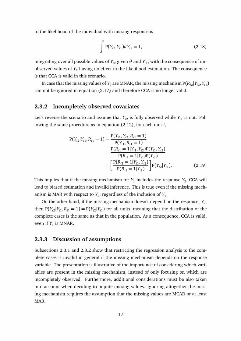
to the likelihood of the individual with missing response is

∫

P(Yi2|Yi1)dYi2 = 1, (2.18)

integrating over all possible values of Yi2 given θ and Yi1, with the consequence of un-

observed values of Y2 having no effect in the likelihood estimation. The consequence

is that CCA is valid in this scenario.

In case that the missing values of Y2 are MNAR, the missing mechanism P(Ri2|Yi2, Yi1)can not be ignored in equation (2.17) and therefore CCA is no longer valid.

2.3.2 Incompletely observed covariates

Let’s reverse the scenario and assume that Yi2 is fully observed while Yi1 is not. Fol-

lowing the same procedure as in equation (2.12), for each unit i,

P(Yi2|Yi1, Ri1 = 1) =P(Yi1, Yi2, Ri1 = 1)

P(Yi1, Ri1 = 1)

=P(Ri1 = 1|Yi1, Yi2)P(Yi1, Yi2)

P(Ri1 = 1|Yi1)P(Yi1)

=

P(Ri1 = 1|Yi1, Yi2)P(Ri1 = 1|Yi1)

P(Yi2|Yi1). (2.19)

This implies that if the missing mechanism for Y1 includes the response Y2, CCA will

lead to biased estimation and invalid inference. This is true even if the missing mech-

anism is MAR with respect to Y2, regardless of the inclusion of Y1.

On the other hand, if the missing mechanism doesn’t depend on the response, Y2,

then P(Yi2|Yi1, Ri1 = 1) = P(Yi2|Yi1) for all units, meaning that the distribution of the

complete cases is the same as that in the population. As a consequence, CCA is valid,

even if Y1 is MNAR.

2.3.3 Discussion of assumptions

Subsections 2.3.1 and 2.3.2 show that restricting the regression analysis to the com-

plete cases is invalid in general if the missing mechanism depends on the response

variable. The presentation is illustrative of the importance of considering which vari-

ables are present in the missing mechanism, instead of only focusing on which are

incompletely observed. Furthermore, additional considerations must be also taken

into account when deciding to impute missing values. Ignoring altogether the miss-

ing mechanism requires the assumption that the missing values are MCAR or at least

MAR.

17

An intrinsic problem of multiple imputation entails that the validity of the assump-

tions for the missing mechanism can not be tested. Taking ignorability for granted

when in fact the data is MNAR will make the inference invalid. Possible remedies

are the inclusion of additional predictors in the imputation models (Schafer, 1997) or

performing a sensitivity analysis (Carpenter and Kenward, 2012).

In this contribution it will be assumed that the missing values are MAR with respect

to the observed variables. In addition, the missing mechanism will generally include

the response, making CCA invalid.

18

Chapter 3

Multiple Imputation

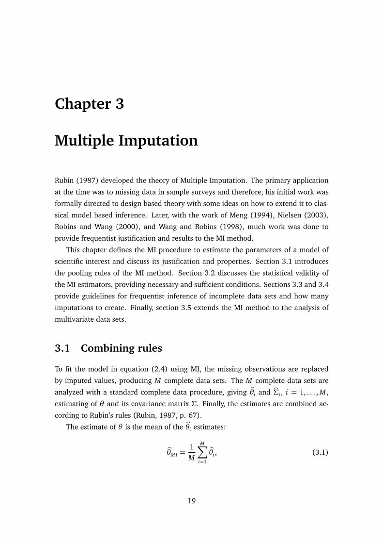
Rubin (1987) developed the theory of Multiple Imputation. The primary application

at the time was to missing data in sample surveys and therefore, his initial work was

formally directed to design based theory with some ideas on how to extend it to clas-

sical model based inference. Later, with the work of Meng (1994), Nielsen (2003),

Robins and Wang (2000), and Wang and Robins (1998), much work was done to

provide frequentist justification and results to the MI method.

This chapter defines the MI procedure to estimate the parameters of a model of

scientific interest and discuss its justification and properties. Section 3.1 introduces

the pooling rules of the MI method. Section 3.2 discusses the statistical validity of

the MI estimators, providing necessary and sufficient conditions. Sections 3.3 and 3.4

provide guidelines for frequentist inference of incomplete data sets and how many

imputations to create. Finally, section 3.5 extends the MI method to the analysis of

multivariate data sets.

3.1 Combining rules

To fit the model in equation (2.4) using MI, the missing observations are replaced

by imputed values, producing M complete data sets. The M complete data sets are

analyzed with a standard complete data procedure, giving bθi and bΣi, i = 1, . . . , M ,

estimating of θ and its covariance matrix Σ. Finally, the estimates are combined ac-

cording to Rubin’s rules (Rubin, 1987, p. 67).

The estimate of θ is the mean of the bθi estimates:

bθM I =1M

M∑

i=1

bθi, (3.1)

19

and the estimate of the covariance matrix Σ is given by:

bΣM I =cW +

1+1M

bB, (3.2)

where cW is the within-imputation covariance matrix

cW =1M

M∑

i=1

bΣi, (3.3)

and bB the between-imputation covariance matrix of bθi

bB =1

M − 1

M∑

i=1

(bθi − bθM I)(bθi − bθM I)T . (3.4)

Rubin (1987) shows that the formulas for the estimators can be justified by writing

the posterior distribution of the θ parameters given the observed data, P(θ |Y obs) as

P(θ |Y obs) =

∫

P(θ |Y obs, Y mis)P(Y mis|Y obs)dY mis, (3.5)

where P(Y mis|Y obs) is the conditional predictive distribution of the missing data given

the observed data and P(θ |Y obs, Y mis) is the posterior distribution of θ given the com-

plete data.

Equation (3.5) suggests that the posterior distribution of θ is the average of the

repeated draws of θ given the completed data (Y obs, Y mis), where Y mis is drawn from

its posterior distribution given Y obs. This is the main reason in favor of MI inference,

since it expresses the posterior of θ given the observed data as the combination of two

simpler posteriors, one being determined by a known complete data procedure and

the other by the imputation model.

The posterior mean of P(θ |Y obs) can be written as

E(θ |Y obs) = E[E(Q|Y obs, Y mis)|Y obs], (3.6)

which can be approximated by equation (3.1), considering that the values bθi are drawn

from P(θ |Y obs, Y mis). Similarly, taking into account that the posterior variance can be

written as

Var(θ |Y obs) = E[Var(Q|Y obs, Y mis)|Y obs] + Var[E(Q|Y obs, Y mis)|Y obs]. (3.7)

The first term in the sum is the average of the variances from the complete data pos-

20

terior bΣi which is estimated by cW . The second component is the variance of the bθi

values and is approximated by bB. The extra term bB/M in the MI variance estimator

in equation (3.2) was introduced by Rubin (1987) and follows from the fact that bθM I

is by itself an estimate for finite M .

3.2 Validity of the MI estimator

Let’s assume that a complete data procedure exists and that it yields estimators bθ andbΣ of the parameter θ and its covariance matrix Σ, for example equations (2.2) and

(2.3). The estimators are said to be statistically valid if

E(bθ |Y )' θ , (3.8)

and

E(bΣ|Y )' Var(bθ |Y ). (3.9)

The objective of the MI approach according to Rubin (1996) is to provide proce-

dures that lead to statistically valid results when applied to incomplete data sets, given

appropriate imputation and analysis models.

If we have an incomplete data set, it’s necessary to consider an extra analysis level

where the MI method is applied. In principle, the idea is to go from the incomplete

data set to a complete sample and then estimate the population parameters. That

means, for example, that bθ is not only an estimator for θ but an estimand for bθM I .

Rubin (1987) defines the concept of “proper imputation” (see also, Rubin, 1996) which

imposes conditions on the imputation procedure that leads to valid estimators bθM I andbΣM I . An imputation procedure is said to be proper if

E(bθM I ,∞|Y obs, Y mis) = E

limM→∞

M∑

i=1

bθi

Y obs, Y mis

' bθ , (3.10)

E(cW∞|Y obs, Y mis) = E

limM→∞

M∑

i=1

bΣi

Y obs, Y mis

' bΣ, (3.11)

and

E(bB∞|Y obs, Y mis) = E

limm→∞

1M − 1

M∑

i=1

(bθi − bθM I)(bθi − bθM I)T

Y obs, Y mis

= Var(bθM I ,∞|Y obs, Y mis) (3.12)

The main result derived from the previous equations is that: if an imputation

21

method is proper for the parameters bθ and bΣ and a complete data procedure based

on such parameters is valid for θ then the inference based on MI estimators for large

M is also valid (Rubin, 1996).

Using equations (3.8) to (3.12) and with the help of the law of iterated expecta-

tions it follows that

E(bθM I ,∞|Y ) = E[E(bθM I ,∞|Y )|Y ]' E(bθ |Y )' θ (3.13)

and

E(bΣM I ,∞|Y ) = E(cW∞|Y ) + E(bB∞|Y )

= E[E(cW∞|Y )|Y ] + E[E(bB∞|Y )|Y ]

' E(bΣ|Y ) + E[Var(bθM I ,∞|Y )|Y ]

' Var(bθ |Y ) + E(Var(bθM I ,∞|Y )|Y )

' Var(E(bθM I ,∞|Y )|Y ) + E(Var(bθM I ,∞|Y )|Y )

= Var(bθM I ,∞|Y ) (3.14)

where Y = (Y mis, Y obs) is the collection of completed data sets. This shows the validity

of the MI based estimators, as long as the assumptions are correct. Obtaining a valid

complete data procedure is usually not a problem in most applications since common

solutions use a OLS estimator. However, having an imputation that is always proper

is not guaranteed. Rubin (1996) suggests that a reasonable imputation method that

satisfies equation (3.12) would tend to satisfy equations (3.10) and (3.11).

On the other hand, Nielsen (2003) argues that the use of Bayesian or approxi-

mately Bayesian predictive distributions to generate imputations is inefficient even if

the method is proper. Meng and Romero (2003) and Rubin (2003) discussed that

issue reasoning that the relationship between the complete data procedure and the

imputation method can not be overlooked. In the critical examples of Nielsen (2003)

the relationship between the analysis and imputation models was ignored.

A simpler explanation is that there must be some connection between the analysis

and imputation models. They can be fitted separately and to some extent, consid-

ered independently from each other, but they are not. The concept of “congeniality”,

introduced by Meng (1994), establishes the required relationship between analysis

procedure and imputation method.

Let Pcom = (bθ , bΣ) denote the complete data procedure, i.e., the statistical proce-

dure that applied to the complete data set estimates the population parameter θ and

its associated variance. Analogously, Pobs = (bθobs, bΣobs) denotes an analysis procedure

based only on the observed data. According to Meng (1994) a Bayesian model f is

22

said to be congenial to the analysis models Pcom,Pobs for a given observed data set

if:

(i) Given the completed data set, Y = (Y obs, Y mis), the analysis model Pcom asymp-

totically gives the same mean and variance estimates as the posterior mean and

variance under f , for all possible values of Y mis, i.e.

E f (bθ |Y ), Var f (bθ |Y )

' (bθ , bΣ) ∀ Y mis, (3.15)

(ii) The posterior mean and variance of θ under f given the incomplete data are

asymptotically the same as the estimate and variance from the partially observed

data model Pobs, i.e.

E f (bθ |Y obs), Var f (bθ |Y obs)

' (bθobs, bΣobs). (3.16)

Then the analysis procedure Pcom,Pobs is said to be“congenial” to the imputation

model g(Y mis|Y obs, A) if there is a Bayesian model f that (i) is congenial to Pcom,Pobsand (ii) the conditional posterior density for Y mis under f is identical to the imputation

model

f (Y mis|Y obs) = g(Y mis|Y obs, A) ∀ Y mis, (3.17)

where A represents possible additional data used in the imputation. This definition es-

tablishes sufficient conditions to obtain proper valid results. If the analysis procedure

is congenial to the imputation model, the MI estimators are valid.

Nielsen (2003) showed that a necessary and sufficient condition for an analysis

procedure to be congenial to an imputation procedure is that the complete data and

observed data estimators are maximum likelihood efficient and their matching vari-

ance estimators are equal to the inverse Fisher information. These results imply that

the congeniality assumption does not hold for some simple estimators, for example,

OLS for heteroscedastic errors. Other cases of uncongeniality can be given when dif-

ferent variables are used in the imputation as those used in the analysis of the scientific

model of interest. Alternative, although computationally more complex variance esti-

mators were proposed by Robins and Wang (2000) and Yang and Kim (2016, Theorem

2).

3.3 Frequentist Inference

Given certain regularity conditions in a congenial setting, MI approximates a full

Bayesian analysis (Carpenter and Kenward, 2012). Since in some fields of applica-

23

tions a frequentist approach is more desirable, we will discuss how to perform fre-

quentist inference on θ , i.e., how to obtain valid estimations of the variance, sampling

distribution and confidence intervals. For a more extensive presentation Chapter 4 of

Rubin (1987) is recommended.

We want to estimate a uni-dimensional parameter θ in our model of interest (2.1).

Let’s assume that the imputation and analysis models are congenial. Applying the

procedure explained in section 3.1 we create M imputed data sets eY mism , Y obs, m =

1, . . . , M using the conditional predictive distribution f (Y mis|Y obs, R) and then use

those data sets to solve the estimating equation in the analysis model to obtain cθm

and bσm.

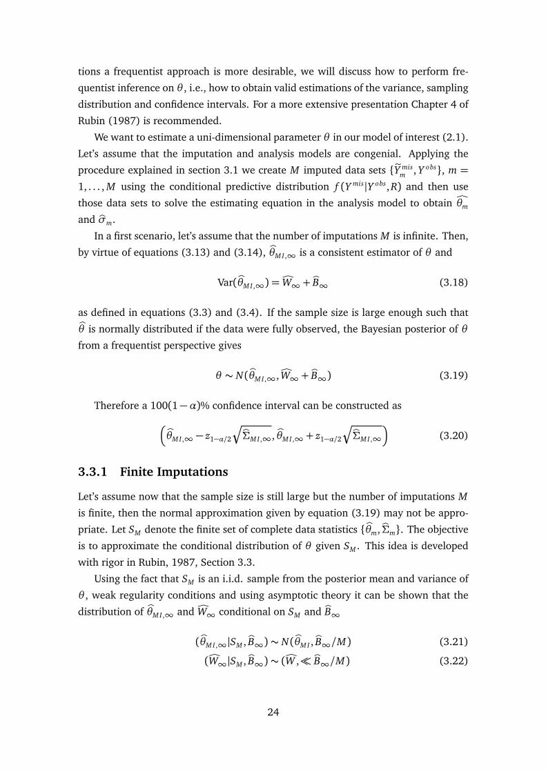
In a first scenario, let’s assume that the number of imputations M is infinite. Then,

by virtue of equations (3.13) and (3.14), bθM I ,∞ is a consistent estimator of θ and

Var(bθM I ,∞) =cW∞ + bB∞ (3.18)

as defined in equations (3.3) and (3.4). If the sample size is large enough such thatbθ is normally distributed if the data were fully observed, the Bayesian posterior of θ

from a frequentist perspective gives

θ ∼ N(bθM I ,∞,cW∞ + bB∞) (3.19)

Therefore a 100(1−α)% confidence interval can be constructed as

bθM I ,∞ − z1−α/2

Ç

bΣM I ,∞, bθM I ,∞ + z1−α/2

Ç

bΣM I ,∞

(3.20)

3.3.1 Finite Imputations

Let’s assume now that the sample size is still large but the number of imputations M

is finite, then the normal approximation given by equation (3.19) may not be appro-

priate. Let SM denote the finite set of complete data statistics bθm, bΣm. The objective

is to approximate the conditional distribution of θ given SM . This idea is developed

with rigor in Rubin, 1987, Section 3.3.

Using the fact that SM is an i.i.d. sample from the posterior mean and variance of

θ , weak regularity conditions and using asymptotic theory it can be shown that the

distribution of bθM I ,∞ and cW∞ conditional on SM and bB∞

(bθM I ,∞|SM , bB∞)∼ N(bθM I , bB∞/M) (3.21)

(cW∞|SM , bB∞)∼ (cW , bB∞/M) (3.22)

24

where, as per Rubin, 1987, Section 2.10, A ∼ (B, C) means that the distribution

of A tends to be centered at B with each component having variability substantially

less than each positive component of C . Combining equations (3.21) and (3.22) with

(3.19) we obtain

θ ∼ N(bθM I ,cW + (1+M−1)bB∞). (3.23)

Using Cochran’s theorem (Cochran, 1934) and by virtue of equation (3.21), the

distribution of bB∞ conditional on SM is proportional to an inverted χ2 random variable

with M − 1 degrees of freedom, that is:

(M − 1)bBbB∞

SM

∼ χ2M−1. (3.24)

Then given SM , the variance in equation (3.23) is the sum of an inverted χ2 and a

constant. That implies that the distribution of θ given SM follows a Fisher-Behrens

distribution. Nevertheless Rubin (1987) provides an approximation of the conditional

distribution of the variance to an inverted χ2, and then formulates the related t dis-

tribution. Specifically, the proposed approximation is:

νcW + (1+M−1)bBcW + (1+M−1)bB∞

SM

∼ χ2ν

(3.25)

being the numerator estimator of the variance, bΣM I as it was defined in equation (3.2),

and ν the degrees of freedom

ν= (M − 1)(1+ r−1M )

2, (3.26)

where

rM =(1+M−1)B

W(3.27)

represents the relative increase in conditional variance due to the missing data (see

Rubin, 1987).

The use of Rubin’s approximation and its variance estimator in equation (3.23)

allows to perform statistical inference about θ using a t distribution with ν degrees of

freedom. For example, a 100(1−α)% confidence interval can be constructed as

bθM I − tv(1−α/2)q

bΣM I , bθM I + tν(1−α/2)q

bΣM I

(3.28)

If θ is a p-dimensional vector, Li, Raghunathan, and Rubin (1991) propose to base

25

the tests on the approximation:

(bθM I − θ )T bΣ−1M I(bθM I − θ )

p(1+ r)∼ Fp,ν′ , (3.29)

where

r =1p

1+1M

tr(bBcW−1),

and

ν′ =

4+ (t − 4)

1+ (1− 2t−1)/r2

if t = p(M − 1)> 4

t(1+ p−1)(1+ r−1)2/2 otherwise.

In the case of a small sample size, where the complete data statistic is already t

distributed, Barnard and Rubin (1999) discuss how to adjust the degrees of freedom.

3.4 Number of Imputations

It has been shown that multiple imputations can yield valid inference, even for values

of M between 3 and 5 (Carpenter and Kenward, 2012; van Buuren, 2012). This

practice is justified analyzing the loss of relative efficiency when using a finite value

of M instead of infinite imputations. The relative efficiency is, approximately

bΣM I =

1+γ

M

bΣM I ,∞, (3.30)

where

γ=rM + 2/(ν+ 3)

rM + 1(3.31)

is the estimated fraction of missing information, with ν and rM given by equations

(3.26) and (3.27) (Rubin, 1987). For example, if the fraction of missing information

is 0.3 and M is set to 5, the estimated variance bΣM I will be only 1.06 times larger thanbΣM I ,∞ yielding a confidence interval just

p1.06= 1.03 times longer than ideal.

The problem with this argument is that, while it is valid in the estimation of θ ,

it doesn’t work the same way when estimating p-values (Carpenter and Kenward,

2012). Graham, Olchowski, and Gilreath (2007) did a simulation study investigating

the effect of M on the statistical power of a test for detecting an effect size of less than

0.1. They found that in order to be closer than 1% of the theoretical power and for

fractions of missing information varying from 0.1 to 0.9, the number of imputations

M must range from 20 to values larger than 100.

Van Buuren (2012) suggests to use a small number of imputations when doing an

exploratory analysis to build the imputation model, and increase M when doing the

26

final analysis.

3.5 Multivariate Missing Data

Real-world data sets with missing values will often have more than one incompletely

observed variable. So far, this chapter has focused on the justification and inferential

aspects of the MI estimator without considerations on how to select and specify the

imputation model. The following sections define the two main approaches available:

Joint Modeling (JM) and Fully Conditional Specification (FCS).

3.5.1 Joint Modeling

Joint Modeling supposes that the data can be described by a multivariate distribution

and assuming ignorability, imputations are created by drawing from said fitted distri-

bution. Common imputation models are based on the multivariate normal distribution

(Schafer, 1997). For simplicity, let’s assume that

Y ∼ N(µ,Σ), (3.32)

where µ= (µ1, . . . ,µp) andΣ a p×p covariance matrix. Taking a flat prior distribution

for µ and a Wp(ν, Sp) prior for Σ−1, if Y were fully observed, the posterior distribution

of (µ,Σ) given Y could be written as the product of

µ|Y,Σ∼ N(Y , n−1Σ) (3.33)

and

Σ−1|Y ∼Wp(n+ ν, (S−1p + S)−1) (3.34)

where Y and (n−1)−1S are the sample mean and covariance matrix respectively (Car-

penter and Kenward, 2012, Appendix B).

If Y is incompletely observed, the estimation of equations (3.33) and (3.34) can be

achieved with the use of the Gibbs sampler as described in algorithm 1. The procedure

will draw parameters in an alternate fashion, conditional on all others and the data.

In the first step the missing data is commonly initialized with a bootstrap sample of the

observed data. After the sampler reached its stationary distribution, multiple imputa-

tions can be generated by taking Y mis?

draws sufficiently spaced from each other. The

“?” symbol denotes that the variable or parameter is a random draw from a posterior

27

Algorithm 1 Joint Modeling Gibbs Sampler1: Fill in missing data Y mis bootstrapping the observed data Y obs

2: Estimate Y and S3: Draw Σ−1

?and µ? using equations (3.34) and (3.33)

4: Draw Y mis?∼ N(µ?,Σ?)

5: Update the estimation of Y and S6: Repeat steps 3 to 5 a large number of times to allow the sampler to reach its

stationary distribution.

conditional distribution.

This methodology is attractive if the multivariate distribution is a good model for

the data but may lack the flexibility needed to represent complex data sets encoun-

tered in real applications. In such cases, the joint modeling approach is difficult to

implement because the typical specifications of multivariate distributions are not suf-

ficiently flexible to accommodate these features (He and Raghunathan, 2009). Also,

most of the existing model-based methods and software implementations assume that

the data originate from a multivariate normal distribution (e.g., Honaker, King, and

Blackwell, 2011; Templ, Kowarik, and Filzmoser, 2011; van Buuren, 2007).

Demirtas, Freels, and Yucel (2008) showed in a simulation study, that imputations

generated with the multivariate normal model can yield correct estimates, even in the

presence of non-normal data. Nevertheless, the assumption of normality is inappro-

priate as soon as there are outliers in the data, or in the case of skewed, heavy-tailed

or multimodal distributions, potentially leading to deficient results (He and Raghu-

nathan, 2009; van Buuren, 2012). To generate imputations when variables in the

data set are binary or categorical, latent normal model (Albert and Chib, 1993) or the

general location model (Little and Rubin, 2002) are also alternatives.

3.5.2 Fully Conditional Specification

Sometimes the assumption of a joint distribution on the data can not be justified, espe-

cially with a complex data set consisting of a mix of several different continuous and

categorical variables. An alternative multivariate approach is given by the Fully Con-

ditional Specification. The method requires the specification of an imputation model

for each incompletely observed variable and impute values iteratively one variable at

a time. This is one of the great advantages of this method, since it decomposes a high

dimensional imputation model into one-dimensional problems, making it a general-

ization of univariate imputation (van Buuren, 2012).

This method is most commonly applied through the Multivariate Imputation by

Chained Equations (MICE) algorithm (van Buuren and Groothuis-Oudshoorn, 2011).

28

This method is summarized in algorithm 2. For each variable with missings a density,

f j(Yj|Yj− ,Θ j), conditional on all other variables is specified, where Θ j are the impu-

tation model parameters. MICE, essentially a MCMC method, visits sequentially each

variable with missings and draws alternately the imputation parameters and the im-

puted values.

Algorithm 2 MICE (FCS)1: Fill in missing data Y mis bootstrapping the observed data Y obs

2: For j = 1, . . . , p

a. Draw Θ?j , from the posterior distribution of the imputation parameters.

b. Impute Y ?j from the conditional model f j(Yj|Yj− ,Θ?j )

3: Repeat step 2 K times to allow the Markov chain to reach its stationary distribution.

The FCS approach splits high-dimensional imputation models into multiple one-

dimensional problems and is appealing as an alternative to joint modeling in cases

where a proper multivariate distribution can not be found or when it does not exist.

The choice of imputation models in this setting can be varied, for example, paramet-

ric models like the Bayesian linear regression, logistic regression, logit or multilevel

models. Liu et al. (2013) studied the asymptotic properties of this iterative imputation

procedure and provided sufficient conditions under which the imputation distribution

converges to the posterior distribution of a joint model.

van Buuren (2012) claims that, in practice, K in step 3 of algorithm 2 can be

set to a value between 5 and 20. This is a strong claim, since usual applications of

MCMC methods require a large number of iterations. The justification is based on

the fact that the random variability introduced by using imputed data in step 2, will

reduce the autocorrelation between iterations in the Markov Chain, speeding up the

convergence.

3.5.3 Compatibility

To discuss the validity of the FCS approach it is necessary to define the term “compat-

ibility” first. A set of density functions, f1, . . . , f j, is said to be compatible if there is

a joint distribution f that generates such set.

The same flexibility of MICE that allows for very special conditional distributions

and imputation models has as a drawback the fact that the joint distribution is not

explicitly known, and there is the possibility that it doesn’t even exists. This is the

case if the conditional distributions specified are incompatible.

Incompatibility in MICE can be the result of imputing deterministic functions of

29

variables in the data along with those same original variables. For example, there

could be interaction terms or nonlinear functions of the data in the imputation models,

introducing feedback loops and impossible combination in the algorithm which would

lead to invalid imputations (van Buuren and Groothuis-Oudshoorn, 2011). For that

reason, the discussion about the congeniality of the imputation and substantive models

is replaced by an analysis of their compatibility.

Although FCS is only justified to work if the conditional models are compatible,

Buuren et al. (2006) reports a simulation study with models with strong incompatibil-

ities where the estimates after performing multiple imputation were still acceptable.

30

Chapter 4

Imputation Methods

Van Buuren (Appendix A, 2012) contains an overview of available MI libraries for

programming languages and statistical software like R, SPSS, SAS, S-Plus and Stata.

Salfran and Spiess (2015) described some of the most common imputation methods

included in these software packages. This chapter provides more details about the

imputing algorithms, incorporating also the methods that will be used later in Chapter

6 in the simulation experiment.

Section 4.1 illustrates the Bayesian Linear regression, one of the older and most

popular methods. Section 4.2 describes Amelia a method published in 2010. Section

4.3 outlines algorithms in the family of Hot Deck imputation methods, like the PMM

approach. Section 4.4 depicts a rather new method based on the software IVEware.

Section 4.5 present a class of imputation methods based on recursive partitioning.

4.1 Bayesian Linear Regression

Imputation by parametric Bayesian regression models is one of the most common

methods of imputation for an univariate variable, Yj, with missing values (Rubin,

1987, see Examples 5.1 and 5.3). It is implemented in practically all imputation soft-

ware packages. It assumes that the posterior density of Yj, f (Yj|ω,η), can be specified

as

Yj ∼ N(ωβ ,σ2) σ > 0, (4.1)

where ω = (1, Yj−), η = (β , log(σ)), β is a vector of j components and σ is a scalar.

If the prior density of η is proportional to a constant and the missing values are MAR

the imputation procedure is given by algorithm 3

Using the theory of generalized linear models (GLM, McCullagh and Nelder, 1989)

the Bayesian Linear Regression model can be also extended through a link function

31

Algorithm 3 Bayesian Linear Regression - Part 1

1: Estimate bβ from the model Yj =ωβ + ε using the observed data.2: Draw X 2, a χ2

nobs− j random variable and let

σ2?=∑

nobs

(Yi j −ωibβ)2/X 2.

3: Draw Z , a N(0, 1) random variable and let

β? = bβ +σ?

∑

nobs

[ωi′ωi]

−1/2

Z

where

∑

nobs[ωi′ωi]

−1/2is the triangular square root obtained by the Cholesky

factorization of∑

nobs[ωi′ωi].

4: Impute Y misj as

Y ?i j =ωiβ? + ξiσ?,

where ξi are independently drawn from a standard normal distribution.5: Repeat steps 2 to 4 M times to generate multiple imputations.

g(·) such as:

E(Yj|ω) = g−1(ωβ) (4.2)

Var(Yj|ω) = v(g−1(ωβ)) (4.3)

where v is a skedastic function of the mean.

In case that g(x) = x and v(x) = σ2, the GLM model is simplified to the linear

regression model in equation (4.1). If for example Yj is a binary variable, then using

a logit link function such as E(Yj|ω) = logit−1(ωβ) equation (4.1) turns into:

Yj ∼ Bernoulli(p), (4.4)

where p = logit−1(ωβ). The imputation algorithm is the same as algorithm 3 except

the actual imputation step, where Y ?i j is a draw from a Bernoulli distribution with

parameter p?i = logit−1(ωiβ?).This imputation procedure is justified by Rubin (1987) and may be expected to

allow valid inferences not only if the assumptions underlying the imputation models

are correct but, due to the “self-correcting” property of MI Little and Rubin (2002) and

Rubin (1987, 1996, 2003), to a certain extent even in more general situations, like

non-linear or non-normal models in the case of continuous Yj or misspecified mean

models in the binary case.

32

4.2 Amelia

Honaker, King, and Blackwell (2011) propose a joint modeling approach in the form

of an imputation method called ‘Amelia II’.

Amelia assumes a normal multivariate distribution for the variables in the data

set, i.e., Y ∼ N(θ ,Σ). The method avoids drawing from the posterior distribution

of the parameters, as in step 2 and 3 from algorithm 3 by combining the bootstrap

(Efron, 1979) with the EM algorithm (Dempster, Laird, and Rubin, 1977). The impu-

tation method is briefly described by algorithm 4. For more details on the expectation-

maximization with bootstrapping (EMB) algorithm see Honaker and King (2010).

Algorithm 4 EMB imputation (Amelia)1: Bootstrap M incomplete data sets.2: Estimate vector Òµi and matrix cΣi, i = 1, . . . , M , using the EM algorithm3: Produce M imputed data sets drawing from N(bµi, bΣi), i = 1, . . . , M .

This imputation algorithm is provided by the R package Amelia. If the variable Yj

to be imputed is non-normal, Honaker, King, and Blackwell (2011) suggest to trans-

form the data to make it look closer to a normally distributed variable. In particular,

if Yj is nominal variable, they propose to impute them as if it were continuous, scale it

into probabilities and draw values for the multinomial distribution using these proba-

bilities.

4.3 Hot Deck Imputation

Hot deck imputation is an alternative to fully parametric methods, which consists of

replacing the missing value with the response of a “similar” observed variable. One

common class of hot deck methods is constituted by k-nearest neighbor (kNN) tech-

niques with advantages that have been discussed by Andridge and Little (2010), Little

(1988), and Schenker and Taylor (1996). The method is simple, it seems to avoid

strong parametric assumptions, only eligible and observed values are imputed, and it

can easily be applied to various types of variables to be imputed.

The idea is to find, for each missing value Yi j, k completely observed neighbors,

somehow close with respect to Yi j− . From this pool of neighbors, one donor is ran-

domly selected and its value Y ?i j is taken as an imputation for Yi j. Closeness is usually

expressed as a distance measure, one popular being based on the estimated condi-

33

tional mean of Yj|Yj− ,

di,i′ =

bE(Y misi j |Yi j−)− bE(Y obs

i′ j |Yi′ j−)

, (4.5)

where Y misi j denotes case i of variable Yj whose value has not been observed, and Y obs

i′ j

denotes case i′ of variable Yj whose value has been observed (i, i′ = 1, . . . , n).

4.3.1 Predictive Mean Matching

When the linear predictor of the regression of Yj onω= (1, Yj−) is used for the distance

in equation (4.5), the imputation technique is also called “predictive mean matching”

(PMM) imputation and goes back to Rubin (1986, 1987) and Little (1988) who coined

the name. The distance function transforms into:

dPM Mi,i′ =

(ωi −ωi′)′β?

, (4.6)

where β? is a random draw from the posterior distribution β in the standard linear

regression model Yj = ωβ . Since the matching is based on the linear predictor and

only observed values are imputed, the method can also be applied to impute non-

continuous variables, e.g., binary variables (van Buuren and Groothuis-Oudshoorn,

2011). Algorithm 5 describes the imputation method.

Algorithm 5 Predictive Mean Matching1: Draw parameter β? from its posterior distribution using steps 1 to 3 of algorithm

3.2: For each missing case i in variable Yj

a. Calculate dPM Mi,i′ for each observed case i′ of variable Yj.

b. Sort the distances and create a set (donor pool) of the first k observed valuesYi′ j with smallest dPM M

i,i′ .

c. Select Y ?i′ j at random from the donor pool.

d. Impute Y ?i j = Y ?i′ j3: Repeat steps 1 and 2 M times to generate multiple imputations.

Under the assumptions that the distance function in equation (4.5) is topologically

equivalent to the Euclidean distance and that k = nr with r ∈ (0,1) as the sample

size n →∞, Dahl (2007) shows that imputations based on kNN techniques can be

interpreted as draws from the conditional distribution of the incompletely observed

34

variable given observed values, that is:

(Y ?j |Ymisj− , Y obs

j )D−−−→n→∞

(Y misj |Y

misj− , Y obs

j )

with bounded correlations

ρ(Y ?j , f (Yj− , Y obsj ))

≤ n1/4,

where f is any measurable function. This means that if the assumptions are true,

the given kNN method will produce imputations with the correct conditional distri-

bution and they will be asymptotically independent over observations. Dahl (2007)

proposes k(n) =p

n as this is ‘canonical in the sense of representing the mid-point of

the interval’ defined by r ∈ (0, 1) (Dahl, 2007, p. 5915).

Convergence rates to the true distribution may vary at different query points, de-

pending on whether regions are thinned out by the response mechanism or not, which

is not the case if the missing data are MCAR, as in the simulation study of Schenker

and Taylor (1996). In addition, mostly all imputation software implementation of the

kNN method provides PMM with k being a parameter that is set to be constant violat-

ing the second assumption. Further, dPM Mi,i′ is not Euclidean, since it can be zero even

if ω 6=ω′.The implementation of PMM in the R package mice uses a slightly different distance

measure, proposed by van Buuren and Groothuis-Oudshoorn (2011),

dM IC Ei,i′ = |ωiβ

? −ωi′bβ |, (4.7)

where bβ is the posterior mean of the parameters of the imputation regression model,

and β? is a draw from the corresponding posterior distribution (Vink et al., 2014).

Two notes are worth mentioning. First, by using observed Yi j values from some

donors as imputations, it is implicitly assumed, that they are random independent

draws from an approximate posterior distribution of Y misj given Y mis

j− . Thus, the as-

sumption is, that the probability of observing Yj given Y misj− is independent of differ-

ences between Y misj− and Y obs

j− , the values of Yj− of completely observed neighbors. Sal-

fran and Spiess (2015) discussed that this is equivalent to assuming, that the missing

data are MCAR within the cells implicitly defined by the k neighbors. Strictly speak-

ing, the assumption is, that the missing data are neither MCAR nor MAR, but missing

locally completely at random (MLCAR).

Second, a special case of kNN imputation is k = 1, i.e. the closest neighbor is the

donor. In this case, there is no random selection of the values to be imputed and even

appropriately taking into account the uncertainty in the parameter estimator of the

35

imputation model does not make this method proper. Thus, k should always be larger

than one.

There has been simulation results implying that PMM versions of kNN imputation

seem to work well (e.g., Andridge and Little, 2010; Vink et al., 2014; Yu, Burton, and

Rivero-Arias, 2007). However, it is not clear if kNN imputation techniques are proper

imputation methods. In fact, Schenker and Taylor (1996) state, that if the number of

possible donors is too small, the M imputations will be correlated leading to a higher

variance of the estimator of interest. On the other hand, increasing the number of

neighbors of a case to be imputed (the query point), may lead to biased estimators due

to a violation of the MLCAR assumption. In a simulation study using fixed (three and

ten) possible donors they found a slight under-coverage of the interesting parameter

of two to three percent. The missing data in their study are MCAR. Similar results

are reported from a simulation study of de Jong, van Buuren, and Spiess (2016) with

missing data being MAR, who found no (obvious) bias but mild to moderate under-

coverage using the kNN imputation method with k = 3.

Most standard analysis software packages or functions offer one of these or a simi-

lar kNN technique, often with a default value for k, like k = 5 (e.g., SAS Institute Inc.,

2015; van Buuren and Groothuis-Oudshoorn, 2011).

4.3.2 aregImpute

Unfortunately, a distance measure based on linear regression models ignores nonlin-

ear effects of Yj− on Yj and may hence still be too restrictive. Thus, a non-parametric

version of kNN imputation provided by function aregImpute as part of the R pack-

age Hmisc has been proposed by Harrell (2015). The suggested algorithm uses the

following distance function:

daregi,i′ =

L∑

l=1

fl(Yi j−)− fl(Yi′ j−)

β?l

, (4.8)

where fl(·), l = 1, . . . , L is a cubic spline basis which lead to optimal prediction, ac-

cording to the coefficient of determination R2, of a linear transformation of Yj in the

following additive model:

c + Yjd = α+L∑

l=1

fl(Yj−)βl + ν

The values of β?l are obtained using a non-parametric bootstrap.

Afterwards, the imputed values are obtained exactly as described in the last part

36

of Algorithm 5, or optionally by randomly selecting a donor from a neighborhood of

the query point with probability inversely proportional to their distance from the ob-

servation with a missing value. For a description, see Harrell (2015) and the literature

cited therein.

4.3.3 MIDAStouch

A rather new method for kNN imputation can be found in the R package midastouch

(Gaffert, Meinfelder, and Bosch, 2016) which is in turn based on MIDAS, a SAS macro

for multiple imputation using distance aided selection of donors (Siddique and Harel,

2009).

Gaffert, Meinfelder, and Bosch (2016) were concerned with the frequentist prop-

erties of the PMM method, specifically a systematic underestimation of the model vari-

ance. They propose a method based on the Approximate Bayesian Bootstrap which

uses a new distance function in combination with bootstrap weights to construct the

donor pool and select the imputed value.

The distance function used is

dM Ti,i′ =

(ωi −ωi′)β?−i′

(4.9)

where β?−i′ is a random draw from the posterior distribution of β−i′ as in the distance

function given by equation (4.6) but following the leave-one-out principle, so β−i′ is

not conditional on the observed case i′.

The donor pool consists of all observed values, defining a probability for every

donor of being used as the imputed value given by

P(Y ?i j = Yi′ j) =νi′d

−κi,i′

∑nobs

i′=1(νi′d−κi,i′ )

(4.10)

where ν denotes non-negative bootstrap weights of the donors, and κ a “closeness”

parameter adjusting the importance of the distance. For a more detailed description

on how to set the bootstrap weights or other parameters, see Gaffert, Meinfelder, and

Bosch (2016).

4.4 Iterative Robust Model-based Imputation

Templ, Kowarik, and Filzmoser (2011) propose an algorithm called ‘Iterative Robust

Model-based Imputation’ (IRMI) implemented in the R package VIM (Alexander Kowarik

and Matthias Templ, 2016). The method copies the functionality of IVEware (Raghu-

37

nathan et al., 2001), modifying the methodology by initializing missing values with

the median and adopting one of several robust estimation methods to reduce the in-

fluence of outlying observations on the regression parameter estimates.

The essence of the method is described by algorithm 6. It can be seen that it is

an imputation procedure like the Bayesian linear regression, but instead of drawing

parameters from their posterior distribution or bootstrapping the observed data set,

they are fixed at their posterior mean and variance. Supposedly the factor multiplying

the estimated variance accounts for the additional uncertainty in the imputations due

to the need of estimating the model, although no justification is given for the value of

this factor.

Algorithm 6 Iterative Robust Multiple Imputation

1: Estimate, using a robust method, bβ from the model Yj = ωβ using the observeddata.

2: Impute Y misj as

Y ?i j =ωibβ +

s

1+nmis

nbσ

where bσ is the robust variance estimator from the residuals in the model.3: Iterate steps 1 and 2 until the imputed values stabilize, i.e., until

∑

nmis

(Y ?,li j − Y ?,l−1i j )< δ

for a small constant δ, where Y ?,li j and Y ?,l−1i j are the imputed values in the l-th and

(l − 1)-th iterations respectively.4: Repeat steps 1 to 3 M times to generate multiple imputations.

The default option for continuous dependent variables in IRMI is the MM-estimator

proposed by Yohai (1987), which is efficient in linear regression models with normally

distributed errors but at the same time largely ignores outliers. The principal prob-

lem of such an automatic method, however, is that it does not differentiate between

valid and invalid outliers. Thus, e.g., if the conditional distribution of a variable to be

imputed is skewed, valid values in a sparsely populated region may be ignored when

the model is fitted. This would lead to estimating the imputation model using system-

atically selective samples and thus to adopting an improper imputation method. The

same arguments apply to the robust imputation techniques for discrete variables.

A limited simulation study presented by Templ, Kowarik, and Filzmoser (2011) is

intended to show the good properties of the technique. However, coverage rates of the

true values in this study range between 0.882 and 0.906, given α= 0.05. In fact, this

imputation method seems not to be proper. In an additional study, imputation tech-

38

niques are evaluated based on comparisons of true but unobserved and imputed val-

ues. With respect to these error measures, the technique proposed in Templ, Kowarik,

and Filzmoser (2011) performs better than an imputation method using Bayesian lin-

ear regression. However, for an imputation method to be proper, it is neither required

nor implied that some measure of distances between true and imputed values is min-

imal (see Rubin, 1987, 1996, 2003). Salfran, Jordan, and Spiess (2016) presented

simulation results showing the method regularly producing larger biases and lower

values of coverage than others methods. At the same time the reported mean square

errors were smaller than the remaining methods.

4.5 Recursive Partitioning

Let’s continue with the incompletely observed variable Yj. Assume that we want to use

Yj = h(Yj−), where h is a model that includes interactions among the Yj− predictors.

The imputation methods described so far allow the use of such a model, although it

would make the matter of congeniality even harder to justify, to the point of getting

uncongenial models if the scientific model of interest does not include such interac-

tions.

An alternative approach is described by Doove, Van Buuren, and Dusseldorp (2014)

who define a new class of non-parametric multiple imputation methods based on Clas-

sification and Regression Tress (CART) or Random Forests (RF) algorithms. These two

methods fall into the umbrella concept of “recursive partitioning”, that allows for the

modeling of internal interactions in the data by sequentially partitioning the data set

into homogeneous subsets. Implementations of both methods for the language R can

be found in the packages mice (van Buuren and Groothuis-Oudshoorn, 2011) and

CALIBERrfimpute (Shah, 2014).

4.5.1 Classification and Regression Trees

CART methods uses a decision tree as a predictive model that represent the observa-

tions Yj− as branches from which conclusions about Yj, the leaves, can obtained. The

kind of tree is determined by the type of target variable, classification trees for discrete

Yj and regression trees for continuous Yj.

Algorithm 7 summarizes the imputation method. It can be seen that the idea is

similar to PMM, where the predictive mean is calculated by a tree model instead of

a regression model, and the donor pool is specified by all observations in the corre-

sponding leave. Note that the fitting step of the algorithm doesn’t specify the kind of

39

Algorithm 7 Classification and Regression Trees

1: Draw a bootstrap sample¦

Y obsj , Y obs

j−

©

of size nobs from¦

Y obsj , Y obs

j−

©

.

2: Fit Y obsj by a tree model h(Yj−) restricted to Y obs

j− .3: For each Y mis

i j , i = 1, . . . , nmis, let Zi j = Y obsi′ j : h(Y obs

i′ j− ) = h(Y misi j ), i′ = 1, . . . , nobs.

4: Draw one donor Y ?i′ j from Zi j.5: Impute Y ?i j = Y ?i′ j.6: Repeat steps 1 to 5 M times to generate multiple imputations.

tree model, allowing the use of any type.

Van Buuren (2012) claims that CART methods are robust against outliers, can deal

with multicollinearity and swekwed distributions, and are able to fit interactions and

nonlinear relationships. Nevertheless, in a simulation study by Doove, Van Buuren,

and Dusseldorp (2014) it is shown that, even if the method is better in some cases

than PMM or the Bayesian Linear Regression when estimating the coefficient of an

interaction term, it fails to reach nominal coverage levels consistently. One the at-

tributed explanations is the sequential nature of the tree models leading to inexact

imputation models due to sub optimal and unstable trees.

4.5.2 Random Forest

Recursive partitioning algorithms, like CART, are commonly criticized for overreacting

to minor changes in the data and tend to overfit the models. Random forests (RF)

are an alternative that differ from CART by constructing a multitude (forest) of tree

models. The objective is to average many decision trees, reducing the variance and

recurrence of unstable trees (Doove, Van Buuren, and Dusseldorp, 2014).

The algorithm needed for RF imputation is a modification of algorithm 7. The

first two steps are replaced by a construction of k bootstrapped data sets, k being the

number of trees in the forest, and the fitting of k tree models. Optionally, each tree can

be fitted using the full bootstrapped data set or randomly selecting the input variables.

To avoid reduced variability by imputing based on an averaged tree, possibly due to

the higher stability of the individual trees, the imputed value is randomly selected

from the union of the k donor pools. For more details on the algorithm see Doove,

Van Buuren, and Dusseldorp (2014, Appendix A)

40

Chapter 5

Robust imputation with GAMLSS and

mice

De Jong (2012) proposed a new imputation technique based on a class of generalized

additive models for location, scale, and shape (GAMLSS), which were introduced by

Rigby and Stasinopoulos (2005). The use of GAMLSS allows the flexible modeling

of the location (e.g., the mean), the scale (e.g., variance), and the shape (e.g., skew-

ness and kurtosis) of the distribution of the incompletely observed variable, given the

observed data.

The original work on the imputation technique was limited since the method was

only able to deal with missings in one variable, the implementation was numerically

unstable, and although it was published by de Jong (2012) and de Jong, van Buuren,

and Spiess (2016) there wasn’t any software library that allowed its use by the general

public. A new R library, named ImputeRobust, was created as part of this thesis,

extending the mice package with a class of GAMLSS imputation functions.

This chapter describes the GAMLSS-based imputation method and the referred

software library. Section 5.1 introduces the required model at the basis of the de-

veloped method. Section 5.2 shows how imputed values are obtained and explains

the algorithm. Section 5.3 provides details of the software and examines how it can

be adjusted. Section 5.4 presents an example of real usage of the ImputeRobust

library. Section 5.5 discusses theoretical considerations and limitations of the impu-

tation method.

5.1 GAMLSS

The assumptions made by the Bayesian linear regression method described in section

4.1 are quite strong, even if extended with the help of generalized linear models. Its

41

most flexible formulation uses a linear prediction function to model the conditional

expectation and variance of the variable with missing values Yj.

The imputation technique developed by de Jong (2012) and de Jong, van Buuren,

and Spiess (2016) also proposes to impute missing values based on a model, not unlike

Bayesian linear regression. The main difference is that instead of assuming a Normal

model in the Bayesian Linear Regression proposed by Rubin (1987), the newer ap-

proach designed by de Jong, van Buuren, and Spiess (2016) uses a model belonging

to the class of GAMLSS (Rigby and Stasinopoulos, 2005).

Let Yj be the variable to be imputed, we assume that

Yj ∼ D(g1(θ1j ) = η1, g2(θ

2j ) = η2, . . . , gK(θ

Kj ) = ηK), j = 1, . . . , n, (5.1)

where D is a parametric distribution with K parameters θ kj , k = 1, . . . , K which are

connected to the additive predictors ηk by the known monotonic link functions gk(·).The parameters (θ 1

j ,θ 2j ,θ 3

j ,θ 4j ) are typically associated with the location, scale,

and shape parameters of the distribution D. The actual value of K determining the

number of parameters depends on the distribution contemplated, being K = 4 the

maximum value considered. It should be clear from the notation that the distribu-

tion parameters are individually associated with each observation of Yj. Finally, the

additive predictors ηk take the form:

ηk = Ωkβk +Lk∑

l=1

hlk, (5.2)

where Ωk is a fixed known design matrix, β Tk a vector of linear predictors, and hlk =

hlk(x lk) is the vector evaluation of a unknown smoothing function hlk of the explana-

tory variables x lk. Equation (5.2) is known as the semi-parametric additive formula-

tion of GAMLSS and for specific combinations of l and k parametric, nonparametric

and random-effects terms could be modeled (Rigby and Stasinopoulos, 2005; Stasinopou-

los and Rigby, 2007).

The model presented relaxes the Bayesian linear regression model as described in

Section 4.1, the latter being just a particular case. If D is taken as the normal distri-

bution and the equation (5.2) is reduced to only a linear predictor, with appropriate

link functions, the model is reduced to the Bayesian linear regression model.

5.2 Imputation

The chosen distribution, D, in model (5.1) defines the type and number of parame-

ters to be modeled. The default distribution was assumed to be normal by de Jong,

42

van Buuren, and Spiess (2016) and de Jong (2012), but other alternatives may be

preferable. In principle, any family implemented in the gamlss package (Rigby and

Stasinopoulos, 2005) can be selected. This close relationship with the gamlss pack-

age is an advantage since a user of the imputation method could adopt any extension

of gamlss to restrict imputations to a certain range, e.g., by specifying a truncated or

censored version of any distribution.

For the default normal distribution, the mean and variance are estimated, but other

distributions may also require the estimation of the skewness and kurtosis. Adopting

models with more parameters increases their flexibility and thus may increase the

chance that the imputation procedure is proper in the sense of Rubin (1987). On

the other hand, larger sample sizes may be needed to identify the larger number of

parameters.

A caveat of the gamlss package is that it does not support Bayesian inference.

Hence it is not possible to obtain multiple imputations by drawing from the posterior

predictive distribution. De Jong, van Buuren, and Spiess (2016) and de Jong (2012)

overcame this issue approximating the predictive posterior distribution by the boot-

strap predictive distribution (Efron, 2012; Harris, 1989):

f ?(Y misj |Y

obsj , Y− j) =

∫

f (Y misj |η, Y mis

− j ) f (η|η(Yobsj , Y obs

− j ))dη , (5.3)

where η denotes the possible values of the imputation model parameters, η(Y obsj , Y obs

− j )is an estimator of such parameters, and f (η|η(Y obs

j , Y obs− j )) is the sampling distribution

of the imputation parameters evaluated at the estimated values. The sampling distri-

bution is simulated with a parametric bootstrap acting as a replacement for the poste-

rior distribution of the imputation parameters. Algorithm 8 shows how the imputation

process is realized after the distributional assumptions are made.

On the other hand, Umlauf, Klein, and Zeileis (2017) developed a conceptional

framework called Bayesian additive models for location, scale, and shape (BAMLSS)

because of the close similarities to GAMLSS. The key difference centers around a crit-

ical component of the fitting algorithm of GAMLSS: the maximization of a penalized

likelihood function of the parametric vectors βk and hyperparameters of the smoothing

terms hlk in equation (5.2). The newly proposed method provides Bayesian analysis

features to GAMLSS by assuming the existence of sensible prior distributions for said

parameters, instead of them being fixed.

The use of BAMLSS opens an alternative way to generate imputations. The method

is very close to GAMLSS but with the selection of particular priors more general model

terms could be defined. Umlauf, Klein, and Zeileis (2017) also created a modular

43

Algorithm 8 GAMLSS imputation

1: Fit model (5.1) using the observed data Y obsj , Y obs

− j obtaining estimates η j1, η j

2,

ηj3 and η j

4.2: Resample Y obs

j as follows:

Y obsj? ∼ D(η

j1, η j

2, η j3, η j

4) .

3: Define a bootstrap sample B = Y obsj? , Y obs

− j 4: Refit model (5.1) using B. This leads to adapted estimates η j

1, η j2, η j

3 and η j4.

5: Impute Y misj as follows:

Y misj ∼ D(η j

1, η j2, η j

3, η j4) .

6: Repeat steps 2 to 5 M times to generate multiple imputations.

computational architecture that is available in the R package bamlss. The driving

concept of the imputation with BAMLSS is the possibility of drawing posterior param-

eters with MCMC sampling. Algorithm 9 describes how imputations with BAMLSS can

be obtained.

Algorithm 9 BAMLSS imputation

1: Fit model (5.1) using the observed data Y obsj , Y obs

− j obtaining estimates η j1, η j

2,

ηj3, and η j

4.2: Draw estimates η j

1, η j2, η j

3 and η j4 using MCMC sampling with estimates η j

1, η j2,

ηj3, and η j

4 as starting points.3: Impute Y mis

j as follows:

Y misj ∼ D(η j

1, η j2, η j

3, η j4) .

4: Repeat steps 2 to 5 M times to generate multiple imputations.

How the two methods compare to each other is something that will be discussed

in the next chapter after the simulation results are presented. A relevant argument is

given by Fushiki (2005) who showed that the bootstrap predictive distribution works

better than the Bayesian predictive if the underlying model in the sampling distribution

is misspecified.

De Jong (2012) and de Jong, van Buuren, and Spiess (2016) presented simulations

results assuming a normal distribution when imputing a single incompletely observed

variable in a bivariate data set. The results were valid even if the variable to be im-

puted was non-normal or counted, except for heavy-tailed distributions where the re-

sults were unsatisfactory and instances where the algorithm failed to imputed values.

Salfran and Spiess (2015) expanded the scope of the initial research and showed that

the good properties hold for more complex missing data structures and multivariate

44

data sets, although with the same problems.

To address the shortcomings of the previous research, Salfran and Spiess (2018b)

published an R package called ImputeRobust. The software library is integrated with

the popular imputation package mice (van Buuren and Groothuis-Oudshoorn, 2011)

increasing its functionality with the inclusion of both GAMLSS and BAMLSS impu-

tation algorithms. The package stabilizes gamlss enough to allow for more flexible

distributions other than the normal with the expectation of improved results. Specifi-

cally, the four-parameter Johnson’s SU distribution was extensively used, allowing for

better results when imputing very asymmetric or leptokurtic data. Also, the package

expands the distribution families provided by bamlss for fitting and MCMC sampling

algorithms. The following section describes its implementation.

5.3 Software Implementation

Two imputing functions, mice.impute.gamlss() and mice.impute.bamlss(), with

the addition of the fitting function ImpGamlssFit() represent the most important

software procedures in the ImputeRobust library (Salfran and Spiess, 2018a,b).

The function ImpGamlssFit() is internal, and its job is to read in the data and

model parameters to create a bootstrap predictive sampling function, i.e., it will work

through steps 1 to 4 of Algorithm 8. The fitting step makes use of the gamlss package

to fit model (5.1) based on (penalized) maximum likelihood estimation and adopt-

ing the default link functions. Rigby and Stasinopoulos (2005) and Stasinopoulos

and Rigby (2007) provide a detailed description of the fitting algorithms and their R

implementation.

For the smoothing functions h jk in the additive predictors given by equation (5.2),

the choice is between cubic splines, penalized splines or local polynomial regression

surfaces. By default, and based on computational stability, we selected P-splines (pe-

nalized B-splines) to construct the smoothing terms. Specifically, the splines consist

of 20 knots, a piece-wise polynomial of second degree, a second order penalty with

smoothing parameters automatically selected using a local Maximum Likelihood cri-

terion. A theoretical explanation of the selected P-splines can be found in Eilers, Marx,

and Durbán (2015).

Even if the P-splines smoothing functions are considered to be stable in the gamlss

package, sometimes the fitting algorithm may diverge. For example, if samples are

too small and the volume of the predictor space gets too large, computational prob-

lems like exploding variances could arise. To prevent abnormal termination of the

algorithm, the complexity of the model is automatically restricted, for instance, the

degree of the polynomial, the order of the penalty, or the stopping time of the fitting

45

algorithm can be reduced.

The user can modify or increase further the degree of model simplification through

optional arguments that can be introduced in the top mice() function call. These

arguments, like cc or cyc, control the convergence criterion or number of cycles of

the inner GAMLSS fitting function, respectively. A more exhaustive description can

be found looking at the auxiliary functions glim.control() and gamlss.control()

provided by the gamlss package (Rigby and Stasinopoulos, 2005).

Alternatively, since the estimation of the distribution parameters is done on an indi-

vidual basis, the computational problems could be reduced to a subset of imputations

with extreme values. Then, instead of decreasing the complexity of the full model,

the simplification could be restricted to the extreme cases. In a worst-case scenario, a

different imputation method can be used for such data points. The Boolean argument

EV can be used to allow for extreme values correction.

The necessary R formula objects for the model are automatically created by the

function during execution time. The default and simplified imputation models can be

controlled with the arguments gam.mod and mod.planb. These take the form of a list

with elements specifying the type of smoother and its parameters. Another way of

adjusting the definition of the models is the lin.terms argument. This last argument

can be used to define which variables should enter model (5.2) linearly.

To improve the stability of the software, distributional parameters can be modeled

as a constant term for all units, i.e. ηk = Ck for some values of k where Ck is a

constant, this is equivalent to say that gk(θ kj ) = Ck for j = 1, . . . , n. The selected family

determines the value of K in equation (5.1) and therefore how many parameters are

to be modeled. The argument n.ind.par sets the maximum number of parameters to

be fitted with the semi-parametric additive model (5.2). For example, if the Johnson’s

SU family (a four parameter continuous distribution) is selected and n.ind.par = 2,

then the mean and the deviation are vectors, but the shape parameters are restricted

to be the same for all units. The numbers of individually fitted parameters in the

simplified model takes the same value as n.ind.par but can be set to a different

value through argument n.par.planb.

The function mice.impute.gamlss() has the same structure as the imputation

methods included in the mice package, meaning that method = "gamlss" is a valid

argument that can be directly passed to the mice() function. As it was established

in the previous section, the normal distribution is the default response distribution

family used by the fitting and imputation methods, but a different distribution family

can be utilized instead by changing the value of the argument family.

For convenience, additional functions are included in the package that are equal

to mice.impute.gamlss() but with family and n.ind.par arguments preset to non-

46

default values. This allows users to mix different gamlss imputation methods within

one call to the function mice(). All functions are variants of mice.impute.gamlss()

where the "gamlss" part is replaced by a method from Table 5.1. The name of

the function is a reference to the corresponding family from gamlss.family (see

Stasinopoulos and Rigby, 2007)

Method Model distributiongamlssNO NormalgamlssBI BinomialgamlssGA GammagamlssJSU Johnson’s SUgamlssPO PoissongamlssTF Student’s tgamlssZIBI Zero inflated BinomialgamlssZIP Zero inflated Poisson

Table 5.1: Included univariate gamlss imputation models.

The function mice.impute.bamlss() is very similar to its gamlss counterpart.

Arguments like gam.mod, lin.terms, n.ind.par, and family are still valid for this

function as a step of the algorithm is the fitting of a GAMLSS model. The argument that

controls the behavior of the MCMC sampler is the fundamental difference. This is done

with propose that sets the propose function for model terms. The default proposal

function is set to "iwlsC" which implies that the smoothing variances of univariate

terms are sampled assuming an inverse gamma prior. A detailed description of the

methods provided by bamlss can be found in Umlauf, Klein, and Zeileis (2017).

5.4 Usage

In what follows, we show with an example how ImputeRobust can be utilized in an

estimation task together with mice. Let us assume that we have a hypothetical data set

with 1000 incompletely observed units and five variables. We desire to estimate the

parameters in the linear regression of one dependent on four independent variables.

The four independent variables (X1, . . . , X4) are weakly correlated and are random

samples from four specific distributions: the standard normal, the Chi-squared, the

Poisson and the Bernoulli distribution, respectively. The dependent variable, Y , is

created according to the linear regression model:

Y = β0 + X1β1 + X2β2 + X3β3 + X4β4 + ε, ε∼ N(0,σ2). (5.4)

47

The vector of linear predictors, β , and the error variance, σ2, are chosen so that the

coefficient of determination, R2, is 0.5.

A non-monotone MAR mechanism dependent on Y and X1 was used to delete

values in X2, X3 and X4. These three variables are missing between 24% and 48% of

their values. Appendix A contains the R code needed to replicate the incomplete data

set.

The imputation task can be performed with a simple call of the mice() function:

> require(ImputeRobust)

> imps <- mice(data, method = c("", "", "gamlssGA", "gamlssPO",

"gamlssBI"), seed = 8913)

iter imp variable

1 1 X.4 X.3 X.2

1 2 X.4 X.3 X.2

1 3 X.4 X.3 X.2

1 4 X.4 X.3 X.2

1 5 X.4 X.3 X.2

2 1 X.4 X.3 X.2

2 2 X.2 X.3 X.4

...

All output is generated by the mice package, for details see van Buuren and Groothuis-

Oudshoorn, 2011. The result is an object of class Multiply Imputed Data Set (mids)

with contents:

> print(imps)

Multiply imputed data set

Call:

mice(data = data, method = c("", "", "gamlssGA", "gamlssPO",

"gamlssBI"), seed = 8913)

Number of multiple imputations: 5

Missing cells per column:

y X.1 X.2 X.3 X.4

0 0 477 461 242

Imputation methods:

y X.1 X.2 X.3 X.4

"" "" "gamlssGA" "gamlssPO" "gamlssBI"

VisitSequence:

X.2 X.3 X.4

3 4 5

48

PredictorMatrix:

y X.1 X.2 X.3 X.4

y 0 0 0 0 0

X.1 0 0 0 0 0

X.2 1 1 0 1 1

X.3 1 1 1 0 1

X.4 1 1 1 1 0

Random generator seed value: 8913

The value of argument method in the mice function call implies that the distribu-

tion assumed is the Gamma for X2, the Poisson for X3, and the Binomial for X4. This

allows for the imputation of realistic values as compared to the default normal dis-

tribution. Nevertheless, the objective of MI is to achieve the statistical validity of the

estimated values (Rubin, 1996). Sometimes it may be better to use a more flexible

model even if the imputed values are “unrealistic”, for example using a distribution

with larger support, or one being continuous when the variable to be imputed is dis-

crete (see de Jong, 2012; de Jong, van Buuren, and Spiess, 2016; Salfran and Spiess,

2015). Figure 5.1 shows the distribution of the original and imputed data with one-

dimensional scatter plots, also known as strip plots.

The model of interest, as per equation (5.4), is the linear regression of Y on X1,

X2, X3, and X4 that created the original data set. The true value of the regression

coefficient is c(1.8, 1.3, 1, -1). The imputed data sets can be analyzed as follows:

> fit <- with(imps, lm(y ~ X.1 + X.2 + X.3 + X.4))

> round(summary(pool(fit)), 2)

est se t df Pr(>|t|) lo 95 hi 95 nmis fmi lambda

(Intercept) 0.28 0.43 0.65 17.02 0.53 -0.62 1.17 NA 0.53 0.48

X.1 1.67 0.23 7.35 10.68 0.00 1.17 2.17 0 0.66 0.60

X.2 1.33 0.14 9.85 7.48 0.00 1.02 1.65 477 0.77 0.72

X.3 0.97 0.14 6.99 9.64 0.00 0.66 1.28 461 0.69 0.64

X.4 -0.92 0.41 -2.24 12.99 0.04 -1.81 -0.03 242 0.60 0.55

5.5 Discussion

The imputation method based on GAMLSS requires the selection of the conditional

distribution D for each of the variables to be imputed. The decision of which distribu-

tion family to use is a problem that could potentially result in deficient imputed values.

49

Imputation number

−10

010

20

0 1 2 3 4 5

y

−3

−2

−1

01

20 1 2 3 4 5

X.1

02

46

810

0 1 2 3 4 5

X.2

02

46

8

0 1 2 3 4 5

X.30.

00.

20.

40.

60.

81.

0

0 1 2 3 4 5

X.4

Figure 5.1: Strip plot of the five variables in the original and the five imputed datasets. Observed data values are blue and imputed data values are red.

There is no theory justifying a “universal” distribution that leads to valid results in all

cases.

De Jong (2012) reports that the misspecification of D can lead to invalid infer-

ences. We think that more malleable models would be more robust to a misspecified

distribution. Therefore, much emphasis has been made in the current iteration of the

GAMLSS imputation algorithm to relax the restrictions imposed on the distribution

employed and increase the complexity of the semi-parametric additive predictors.

The nonparametric part of model (5.2) makes the "curse of dimensionality" is par-

ticularly relevant for this imputation method. The additive specification allows to in-

corporate many predictors in the model, but possible interactions between them may

be ignored unless explicitly included.

Some computational problems, dependent on the sample size, degree of smooth-

ing, number of predictors in the model and other factors, will always be hard to fore-

see. In general, small data sets with several variables to be imputed might be ill-suited

50

to be treated with the algorithm. In this regard, the most obvious symptoms of issues

are manifested as outliers in a set of imputed values, which may lead to a biased esti-

mation. With the higher flexibility allowed, some responsibility is put on the imputer

to explore the results obtained.

51

Chapter 6

Simulation Experiment

In this chapter, the simulation experiments designed to explore the performance of

the imputation methods described in Chapters 4 and 5 are described.

The multiple imputation techniques described in Chapter 4 take advantage of Ru-

bin’s (1987) work, and they all share the property that no proof exists showing that

inferences based on the multiply imputed data sets are valid in all situations of poten-

tial interest. The properties of scientifically interesting estimators based on multiply

imputed data sets can therefore systematically be studied only in simulation experi-

ments.

De Jong (2012) compared the version of his GAMLSS imputation algorithm to the

Bayesian Linear regression algorithm (Section 4.1), PMM (Section 4.3.1) and aregIm-

pute (Section 4.3.2). His results show that these three methods were sensible to model

misspecification. In any case, recent approaches to missing value compensation still

develop and propose to use these methods or derivatives of them, PMM in particular

(e.g., Gaffert, Meinfelder, and Bosch, 2016; Morris, White, and Royston, 2014; Tutz

and Ramzan, 2014). Salfran and Spiess (2015) presented simulation results testing

the mentioned methods with different experimental conditions. They also included

most of the imputation methods described in Chapter 4 and GAMLSS.

6.1 Experimental Design

The goal of the simulation study is to explore if the inference based on multiply im-

puted data sets is valid under various experimental conditions. All simulation cases

focus on the estimation of the coefficients in a linear regression model when the predic-

tor variables are incompletely observed. This a particular case of the scientific problem

of interest discussed in Chapter 2. We decided to concentrate on this model for the

simulations because we intended to partly replicate the results of de Jong (2012) and

52

de Jong, van Buuren, and Spiess (2016). Though, we extended the scope of the orig-

inal design to encompass more realistic research situations and test the imputation

algorithm with more general data sets.

All simulations were run with R (R Core Team, 2017). Algorithm 10 provides an

outline of how the simulations are done. The various experimental conditions are

controlled according to steps 1 and 2 of the algorithm. These distinct settings can be

divided into several groups which will be discussed in the next sections.

Algorithm 10 Simulation experiment1: Generate the data set.2: Delete values according to a missing data mechanism.3: Multiply impute the incomplete data set using different imputation techniques.4: Calculate point and variance estimates for the coefficients of a linear regression

using the initially complete data set, the completely observed part and the multiplyimputed data set.

5: Repeat steps 1-4 N times.

The imputation methods used in step 3, are the same as described in chapters 4

and 5. Table 6.1 summarizes the methods employed and the corresponding R library

that provides them. Like Salfran and Spiess (2015) also did, we include diverse copies

of the PMM method with different values of donors (1, 3, 5, 10 and 20). The square

root of the sample size is also considered as the number of donors (see Dahl, 2007).

To check the current state of the GAMLSS imputation software modifications, we also

evaluated several copies of the algorithm with different distribution families or fitting

parameters. All other methods use their default settings.

After the simulations are done we calculate the means of the estimates, the positive

square root of the mean of variance estimates, the sample variance of the estimates

over the simulations, and the proportion of cases for which the confidence intervals

Table 6.1: List of tested imputation methodsMethod library (version)Bayesian Linear Regression mice (2.46.0)Amelia Amelia (1.7.4)Predictive Mean Matching mice (2.46.0)aregImpute Hmisc (4.0-3)MIDAStouch mice (2.46.0)IRMI VIM (4.7.0)CART mice (2.46.0)Random Forest mice (2.46.0)GAMLSS imputation ImputeRobust (1.2)

53

cover the true value. The assessment of the quality of the imputation methods is based

on four criteria:

• Bias, being the difference between the mean of the estimators of the regression

coefficient and the known true value. It should be as close as possible to 0.

• Coverage, based on the proportion of 95% confidence intervals covering the true

value. Every simulation could be thought of as an independent random draw of

a binary variable taking on the value one if the confidence interval covers the

true value and zero otherwise. When all assumptions are met, 95% confidence

intervals cover the true parameter value with probability 0.95. This means, for

example, that if 1000 simulations are performed, the coverage rate over the sim-

ulations should be in the confidence interval [0.936, 0.964]. The ideal result is if

mean estimates are approximately unbiased with coverage within the above lim-

its. Under-Coverage (values below the interval) indicates an invalid inference.

Over-Coverage with an unbiased estimator illustrate what’s called confidence

validity (Rubin, 1996).

• Efficiency, as a measure of the standard deviation of the estimators over the

simulations. It is calculated by taking the positive square root of the mean of

the estimated variances in the simulations. While the bias and coverage de-

termine the validity of the imputation method, we are interested in the overall

performance of the imputation methods. This is an auxiliary benchmark. If two

imputation methods are equally valid, the one with smaller variance should be

preferred.

• Relative efficiency, given as the ratio of the mean variance estimates and the

sample variance across simulations. This criterion contrasts the values of Ru-

bin’s variance estimator with the estimated variance over the simulations. The

ideal result is a ratio close to 1. Values below or above 1 are symptoms of un-

derestimation or overestimation of the variance. Likewise the efficiency this is

a secondary criterion.

6.1.1 Single predictor

The first experimental condition partly includes and replicates the “simple design”

used by de Jong (2012) and de Jong, van Buuren, and Spiess (2016). The data gen-

erating process (DGP) is based on the linear regression given by

y = β0 + β1 x + ε, ε∼ N(0,σ2), (6.1)

54

where β0 = 0 and β1 = 1. Three parameters are modified to generate diverse simu-

lations situations. These are the distribution of x , the coefficient of determination R2,

and the sample size n.

The distribution of the predictor variable x can be any option between a standard

normal, a skew-normal with shape parameter λ = 5, uniform between 0 and 1, a

squared uniform (beta), student’s t with ν= 3 degrees of freedom, a Poisson with rate

parameter λ = 3, or a chi-squared with k = 3 degrees of freedom. The value of R2 is

0.25, 0.5, or 0.75 and is adjusted with the variance σ2 of the error in the linear model

once a distribution is selected. The sample size, n, varies between 50, 200, and 1000

units.

Every possible combination of distribution, coefficient of determination and sam-

ple size is analyzed. Each study is simulated N = 1000 times and m= 10 imputations

are realized for each replication. All distributions but the chi-squared were consid-

ered by de Jong (2012). The present design changes besides the rate parameter of the

Poisson distributed variable and the sample sizes. Considering 50 units instead of 500

makes more sense in psychological applications where the sample size is often small.

Also, it is a harder test for the stability of the GAMLSS imputation method.

For all cases, roughly 40% of x is deleted according to the missing data mechanism

(MDM):

P(R= 0|y) =

0.3 if y ≤ y

0.9 a.o.c.(6.2)

where y is the sample median. This means that x is MAR with respect to y , with

probability of being missed equal to 0.3 if y is below the median and 0.9 otherwise.

The strength of the MAR mechanism is dependent on R2 with higher values leading

to more selective thinning out of the sample space. This MDM is exactly the one that

de Jong (2012) and de Jong, van Buuren, and Spiess (2016) utilized.

6.1.2 Multivariate set

We extended the scope of the first experiment by moving into the analysis of multi-

variate data set with multiple incompletely observed variables. The main reason for

this is to test the robustness of the latest version of ImputeRobust in a more realistic

scenario. Besides the multivariate data sets, we also test for the effects of different

missing mechanisms and patterns of missingness. For this, we define two MDM with

a differing selectivity of the region from which values are deleted that we call “strong”

and “weak MDM.” Further, the missing pattern can be either monotone or not. The

combination of MDM and missing pattern applied to every multivariate data set define

55

the four remaining experimental conditions tested.

The DGP chosen to simulate the multivariate data set is similar to the one already

used in the example of Section 5.4. It is based on the linear regression of four corre-

lated covariates (x1, . . . , X4) and normally distributed homoscedastic errors. In each

simulation, the distributions of x1, X3 and X4 are fixed to be the standard normal, the

Poisson with rate parameter λ = 3, and the Bernoulli with mean parameter π = 0.4,

respectively. The distribution of X2 is continuous and may vary between a standard

normal, a chi-squared or a student’s t, these last two with 3 degrees of freedom each.

The four covariates are weakly correlated according to the correlation matrix:

1 0.15 0.1 −0.1

0.15 1 0.25 0.05

0.1 0.25 1 0

−0.1 0.05 0 1

(6.3)

To create the correlated structure, a sample from a four-dimensional multivariate nor-

mal distribution with mean zero and correlation matrix given by (6.3) is drawn. This

is transformed to the desired sample by calculating the values of the standard normal

cumulative distribution function (CDF) for each simulated value and then using the

inverse CDF corresponding to each target distribution.

A dependent variable y is generated according to the linear regression model,

yi = β0 + x i1β1 + x i2β2 + x i3β3 + x i4β4 + εi, εi ∼ N(0,σ2). (6.4)

As with the simple experiment the sample size is either 50, 200 or 1000 units. The true

values of the parameters weighting the predictors change depending on the distribu-

tion of X2, but are fixed at the beginning of each simulation experiment. If X2 follows

a standard normal distribution the vector of parameters is β = (0, 1.3,1.5, 0.8,2.5).If X2 follows instead a t distribution then β = (0,1, 1,0.95, 1.5). Finally, if X2 comes

from a chi-squared distribution then β = (0,2, 1.1,1.5, 4). The difference in regres-

sion coefficients is due to the desire of keeping the effect of each predictor at the

same level, as measured by the partial eta-squares. The error variance σ2 is chosen so

that the coefficient of determination, R2, equals 0.5. The code in Appendix A can be

adapted to get the desired DGP.

We define two MAR mechanism that deletes values on X2, X3 and X4 dependent

on y and x1. The two mechanisms are called “strong” and “weak MDM.” Under both

conditions, the probabilities of not observing a value are the same, being 0.45 for

X2, 0.31 for X3, and 0.079 for X4, leading to a similar proportion of missing values.

The difference consists in the reduction of the selectivity, that is, the “strong MDM”

56

deletes values in one specific region of the space more aggressively as compared to the

“weak MDM.” Figures 6.1 and 6.2 show this difference. In the first one, it can be seen

that values on the right half side of the distribution of the variables are systematically

deleted. On the other hand, in the second case values are more evenly deleted on both

sides.

Let Ri j be the response indicator of x i j, where Ri j = 1 if x i j is observed and Ri j = 0

if x i j is missing. In the first part of the remaining simulation experiments, we es-

tablish monotone missing patterns to avoid possible incompatibility issues, e.g., the

non-existence of a regular distribution of the variables with missing values or numer-

ical issues concerning convergence of the MICE algorithm. This is achieved by condi-

tioning the MDM of a variable to the response indicator R of the previous one. First,

calculate the value r?i = 2yi + x i1, then under the “strong MDM” conditions, values of

X2, X3 and X4 are deleted according to the following rules:

P(Ri2 = 0|r?i ) =

0.1 if r?i ≤ r?0.5

0.8 elsewhere, (6.5)

P(Ri3 = 0|r?i , Ri2 = 0) =

0.68 if r?i ≤ r?0.3

0.71 elsewhere, Pr(Ri3 = 0|r?i , Ri2 = 1) = 0 (6.6)

P(Ri4 = 0|r?i , Ri2 = 0, Ri3 = 0) = 0.25, Pr(Ri4 = 0|r?i , Ri3 = 1) = 0 (6.7)

where r?p is the p-quantile of the r? values. In equations (6.7) points out that R4 is

MCAR given r?, R2 and R3. For the “weak MDM” equations (6.5) and (6.6) turn into:

P(Ri2 = 0|r?i ) =

0.35 if r?i ≤ r?0.5

0.55 elsewhere, (6.8)

P(Ri3 = 0|r?i , Ri2 = 0) =

0.695 if r? ≤ r?0.4

0.703 elsewhere, Pr(Ri3 = 0|r?i , Ri2 = 1) = 0 (6.9)

and the missings values for X4 are still generated according to equation (6.7). Since

the parameters in the DGP and MDM do not depend on each other, and the mecha-

57

0

5

10

15

−2 0 2

r∗

x 2 obs

miss

0

1

2

3

4

5

6

7

8

9

−2 0 2

r∗

x 3

obsmiss

0

1

−2 0 2

r∗

x 4

obsmiss

−10

0

10

20

0 10 20β0 + x1β1 + x2β2 + x3β3 + x4β4

y obsmiss

Figure 6.1: Scatter plot of the missing and observed values using example data fromsection 5.4. From left to right and from top to bottom: chi-squared (X2), Poisson (X3),Binomial (X4) and dependent (y) variables. The independent variables are plottedagainst the linear response tendency function r?. The dependent variable against thelinear predictor β × X . Values are missing according to the “strong” mechanism.

nisms are MAR, both missing mechanisms are ignorable.

An objective of the current work is to actually test the developed and existing

imputation methods in a scenario as realistic as possible. Thus, in the final part of the

simulation experiments we decided to drop the restriction on the monotonicity of the

MDM. We use two non-monotone missing mechanisms derived from the “strong” and

“weak MDM”. In short, the dependency on whether the previous value is observed or

not is dropped. The “strong MDM” becomes:

P(Ri2 = 0|r?i ) = P(Ri3 = 0|r?i ) =

0.1 if r?i ≤ r?0.5

0.8 elsewhere, Pr(Ri4 = 0|r?i ) = 0.25,

and the “weak MDM”:

P(Ri2 = 0|r?i ) = P(Ri3 = 0|r?i ) =

0.35 if r?i ≤ r?0.5

0.55 elsewhere, Pr(Ri4 = 0|r?i ) = 0.25.

58

0

5

10

15

−2 0 2

r∗

x 2 obs

miss

0

1

2

3

4

5

6

7

8

9

−2 0 2

r∗

x 3

obsmiss

0

1

−2 0 2

r∗

x 4

obsmiss

−10

0

10

20

0 10 20β0 + x1β1 + x2β2 + x3β3 + x4β4

y obsmiss

Figure 6.2: Scatter plot of the missing and observed values using example data fromsection 5.4. From left to right and from top to bottom: chi-squared (X2), Poisson (X3),Binomial (X4) and dependent (y) variables. The independent variables are plottedagainst the linear response tendency function r?. The dependent variable against thelinear predictor β × X . Values are missing according to the “weak” mechanism.

6.2 Single Predictor Results

In what follows the results of the simulation study described in section 6.1.1 are pre-

sented. The outcome of the experiments is summarized as shown in table 6.2.

Table 6.2: Example of resultsn= 50 n= 200 n= 1000

bias cov sd ratio bias cov sd ratio bias cov sd ratioR2 = 0.25

COM 0.002 0.956 0.254 1.023 0.004 0.958 0.123 1.026 0.001 0.945 0.055 0.986CCA -0.147 0.934 0.320 0.972 -0.122 0.878 0.153 1.005 -0.126 0.543 0.068 0.933NORM -0.068 0.960 0.346 1.056 -0.008 0.961 0.156 1.038 -0.004 0.944 0.069 0.985AMELIA -0.017 0.941 0.343 0.996 0.006 0.956 0.155 1.036 -0.002 0.941 0.068 0.983PMM-1 -0.040 0.939 0.375 0.970 -0.000 0.900 0.156 0.851 -0.003 0.896 0.066 0.826. . . . . . . . . . . . . . . . . . . . . . . . . . . . . . . . . . . . . . .

Note: If n= 50, results for aI-kNN are based on 373, those for aI-W on 372 successful simulations.

The first column shows the tested methods. The complete data set and complete

case analysis are described as COM and CCA respectively. These are followed by NORM for

59

Bayesian Linear Regression (section 4.1) and AMELIA (section 4.2). Next, several vari-

ants of hot deck imputation methods (section 4.3) are included, in particular, copies

with a different number of donors for the Predictive Mean Matching. These PMM vari-

ants are presented as PMM-N, where N is either 1, 3, 5, 10, 20 or D (meaning the square

root of the sample size). AregImpute and Midastouch are given by AREG and MIDAS

respectively. The Iterative Robust Model-Based Imputation method (section 4.4) fol-

lows the list as IRMI. The recursive partitioning methods (Section 4.5 are included as

CART for classification and regression trees and RF for random forests. Finally, the list

is completed with differing alternatives of GAMLSS imputing methods: BAMLSS and

GAMLSS (both assuming a Normal distribution for the response variable), and GAMLSS-

JSU testing the assumption of the four parameters Johnson’s SU distribution for the

response variable (see chapter 5.1 for details).

The following twelve columns are divided into three groups of four, for each of

the tested sample sizes: 50, 200 and 1000. The four columns in each group report

the four criteria defined in section 6.1. The first column, indicated as bias, shows

the estimated mean bias of the imputation method. A gray gradient is used as the

background for the cells, starting in white for an estimated bias of 0 and getting darker

as it increases. The second column, indicated as cov, contains the coverage probability

of the imputation methods. Values in the acceptable range are colored green, under-

coverage is red and over-coverage, which is confidence valid is orange. The third

column, indicated by sd, presents the efficiency of the estimators. Finally, the fourth

column, denoted ratio, shows the values of relative efficiency between the mean

variance of the estimators and estimated variance across simulations.

The results for the different values of coefficient of determination are included in

the same table. In the first column a line with the text R2 = 0.25, 0.50 or 0.75 is

included to indicate said value.

6.2.1 Normal

The first simulation experiment adopts a normal distribution for the predictor vari-

able. Figure 6.3 represents the effects of the MDM given by equation (6.2) on the

distribution of the missing values where it is shown that the MDM selectively removes

observed values on one side of the data set. This simple condition is meant to serve

as a standard for all imputation methods. Table 6.3 presents the full results of this

simulation study.

Since the MDM is MAR, CCA is expected to fail, and in fact, it does. Regardless

of the value R2 complete case analysis leads to invalid results due to under-coverage

60

−2

0

2

−2 0 2y

X

−5.0

−2.5

0.0

2.5

5.0

−2 0 2X

y

Figure 6.3: Scatter plots of both the direct and reverse regression when the covariateis normally distributed. The red circles are observed values, and the blue triangles aremissing. The coefficient of determination is 0.5.

with values ranging between 0.434 and 0.554 for n = 1000. With increasing sample

size the under-coverage problem only gets worse.

A quick glance at the table shows that the smallest sample size produces the largest

biases while at the same time it contains the largest proportion of methods with cov-

erage in the valid or confidence valid range. This result can be explained by the large

overestimation of the variances. This is known as the “self-correcting” property of

Multiple Imputation (Rubin, 2003) which is a form of compensation for the missing

information.

NORM results are almost perfect in all three cases. This is no surprise since X and y

are bivariate normally distributed fulfilling all required assumptions of the Bayesian

Linear Regression imputation method. The only virtual difference between this impu-

tation method and the analysis with COM is the larger standard errors which in the case

of R2 = 0.5 and n = 50 leads to over-coverage (cov = 0.966). AMELIA also relies on

normality assumptions and in this simple scenario should perform well. The results

are almost as good as NORM, but when R2 = 0.5 and n = 1000 it does suffer from

under-coverage.

There is a general pattern to the PMM methods. If we fix the number of donors

and increase the sample size, i.e., we move in a horizontal line in the table, the bias

of the imputation methods decreases, as do the mean estimated standard errors. The

problem is the drop in coverage probabilities leaving almost no valid PMM method for

n= 200 and none for n= 1000 (cov≤ 0.909). The standard errors are similar to NORM

but the ratio between the mean variance and estimated variance across simulations is

smaller. This indicates that the estimated variances decrease too fast in comparison

to the true variance, and it may explain the under-coverage. Moving in the other

direction, i.e., fixing the sample size and increasing the number of donors, there is not

61

a perfect monotone relationship concerning bias and coverage. For a larger number of

donors, the bias increases but coverages start getting better up to a maximum and then

decrease again. For example, when R2 = 0.25 from 1 up to 10 donors the coverage

increase, and then for 20 andp

1000 ≈ 31.6 donors decrease again. Practically, only

when n= 50, most PMM methods can provide estimates with valid coverage, thanks to

the “self-correcting” property and at the expense of large biases.

AREG and MIDAS perform similar to each other, being the former the best of the

two for R2 = 0.25 and R2 = 0.75 and the latter the best if R2 = 0.5. Both methods

are almost unbiased for n ≥ 200 but suffer from under-coverage and are thus invalid

(cov ≤ 0.933). The only valid cases are provided by MIDAS when n= 50.

IRMI is the worst method overall with extreme results of bias and under-coverage,

being this latter statistic close to 0 for n = 200 and 0 for n = 1000. The standard

errors and the ratio constitute the largest values of these measures of all imputation

methods. The results are evidence of a severe issue in the theory or implementation

of this method. They may be caused by the wrong classification of “extreme” values

which are just outliers due to the thinning of regions with the MDM.

CART and RF perform almost identical to each other in terms of all considered

measures. Both methods suffer from under-coverage although the estimated bias is

relatively non existent. RF leads to valid results only in two cases, for n = 50 and

R2 ≥ 0.5.

Next in the list of imputation methods are the GAMLSS algorithms. The BAMLSS

method suffers from under-coverage and fails to be valid (cov ≤ 0.927). As the sam-

ple size increases the method becomes unbiased, and it shows the smallest standard

error of all imputation methods. A ratio of variances being approximately 0.86 implies

a systematic underestimation of the error. Both GAMLSS and GAMLSS-JSU are unbiased

and provide valid estimation or confidence valid in the case of the Johnson’s SU al-

ternative when R2 = 0.75 and n ≥ 200. They have the largest standard errors, after

IRMI, with GAMLSS-JSU producing the greater values of the two.

The difference between BAMLSS and GAMLSS is the use of the MCMC sampling to

simulate the Bayesian posterior and the Bootstrap Predictive Sampling. Seeing the

different results concerning the validity and the estimated errors and ratio statistics, a

reason for the problem of BAMLSS may be a lack of variability in the MCMC sampling

step of algorithm 9.

Table 6.3: Normal distribution

method n=50 n=200 n=1000

bias cov sd ratio bias cov sd ratio bias cov sd ratio

62

Table 6.3: Continuation of table on previous page

method n=50 n=200 n=1000

bias cov sd ratio bias cov sd ratio bias cov sd ratio

R2 = 0.25COM 0.002 0.956 0.254 1.023 0.004 0.958 0.123 1.026 0.001 0.945 0.055 0.986CCA -0.147 0.934 0.320 0.972 -0.122 0.878 0.153 1.005 -0.126 0.543 0.068 0.933NORM -0.068 0.960 0.346 1.056 -0.008 0.961 0.156 1.038 -0.004 0.944 0.069 0.985AMELIA -0.017 0.941 0.343 0.996 0.006 0.956 0.155 1.036 -0.002 0.941 0.068 0.983PMM-1 -0.040 0.939 0.375 0.970 -0.000 0.900 0.156 0.851 -0.003 0.896 0.066 0.826PMM-3 -0.079 0.927 0.348 0.935 -0.010 0.916 0.153 0.890 -0.004 0.900 0.066 0.860PMM-5 -0.114 0.939 0.342 0.950 -0.017 0.918 0.152 0.901 -0.005 0.906 0.066 0.864PMM-10 -0.190 0.935 0.346 1.035 -0.037 0.930 0.153 0.910 -0.009 0.908 0.066 0.877PMM-20 -0.314 0.907 0.358 1.229 -0.082 0.914 0.156 0.953 -0.018 0.898 0.065 0.868PMM-D -0.143 0.936 0.343 0.976 -0.054 0.931 0.153 0.922 -0.027 0.889 0.066 0.874AREG -0.177 0.919 0.387 0.928 -0.040 0.941 0.169 0.933 -0.013 0.923 0.068 0.892MIDAS -0.059 0.957 0.373 1.036 -0.016 0.936 0.166 0.966 -0.012 0.919 0.072 0.906IRMI -0.424 0.890 0.369 1.580 -0.417 0.278 0.177 1.701 -0.430 0.000 0.078 1.574CART -0.040 0.935 0.306 0.926 -0.007 0.885 0.139 0.808 0.002 0.884 0.061 0.781RF -0.043 0.923 0.311 0.870 0.009 0.895 0.140 0.816 0.010 0.878 0.061 0.793BAMLSS -0.077 0.841 0.294 0.697 0.012 0.927 0.140 0.886 0.001 0.892 0.062 0.861GAMLSS -0.002 0.925 0.377 0.963 0.029 0.954 0.168 1.013 0.005 0.945 0.072 0.989GAMLSS-JSU 0.004 0.936 0.406 1.031 0.042 0.947 0.174 1.061 0.010 0.939 0.073 0.989

R2 = 0.50COM 0.001 0.956 0.146 1.023 0.003 0.958 0.071 1.026 0.001 0.945 0.032 0.986CCA -0.103 0.911 0.193 0.958 -0.085 0.841 0.092 0.986 -0.087 0.434 0.041 0.916NORM -0.030 0.966 0.194 1.061 -0.004 0.960 0.085 1.028 -0.001 0.936 0.037 0.971AMELIA 0.008 0.959 0.187 1.025 0.006 0.946 0.084 1.015 0.000 0.929 0.037 0.974PMM-1 0.006 0.926 0.191 0.894 0.008 0.898 0.080 0.846 0.000 0.880 0.035 0.802PMM-3 -0.022 0.935 0.196 0.914 0.003 0.914 0.081 0.871 -0.000 0.892 0.035 0.820PMM-5 -0.049 0.939 0.202 0.939 0.001 0.917 0.083 0.881 -0.001 0.894 0.035 0.835PMM-10 -0.111 0.939 0.219 1.052 -0.011 0.923 0.085 0.900 -0.002 0.897 0.036 0.839PMM-20 -0.240 0.893 0.242 1.240 -0.040 0.918 0.091 0.954 -0.005 0.898 0.036 0.855PMM-D -0.075 0.941 0.210 0.992 -0.022 0.923 0.088 0.921 -0.009 0.897 0.037 0.857AREG -0.113 0.932 0.242 0.923 -0.017 0.925 0.091 0.904 -0.005 0.893 0.036 0.851MIDAS -0.017 0.962 0.216 1.046 0.003 0.933 0.092 0.964 -0.001 0.926 0.040 0.911IRMI -0.394 0.787 0.264 1.790 -0.395 0.025 0.126 1.866 -0.407 0.000 0.056 1.698CART -0.052 0.944 0.189 0.994 -0.005 0.885 0.080 0.828 0.001 0.881 0.035 0.804RF -0.025 0.946 0.187 0.940 0.008 0.900 0.080 0.864 0.007 0.876 0.035 0.809BAMLSS -0.062 0.849 0.173 0.565 0.008 0.914 0.079 0.889 0.002 0.911 0.035 0.875GAMLSS 0.001 0.942 0.234 0.974 0.019 0.948 0.093 1.065 0.004 0.940 0.040 1.010GAMLSS-JSU 0.004 0.953 0.257 1.123 0.025 0.958 0.098 1.109 0.007 0.941 0.041 0.998

R2 = 0.75COM 0.001 0.956 0.085 1.023 0.001 0.958 0.041 1.026 0.000 0.945 0.018 0.986CCA -0.055 0.933 0.118 0.981 -0.045 0.867 0.055 0.987 -0.045 0.554 0.025 0.935NORM -0.006 0.961 0.112 1.031 -0.001 0.954 0.052 1.028 -0.000 0.945 0.023 0.999AMELIA 0.015 0.956 0.108 1.003 0.004 0.952 0.051 1.022 0.000 0.947 0.023 0.994PMM-1 0.027 0.894 0.108 0.863 0.012 0.882 0.048 0.826 0.002 0.883 0.022 0.807PMM-3 0.020 0.931 0.118 0.962 0.013 0.923 0.049 0.876 0.003 0.901 0.022 0.842PMM-5 0.006 0.957 0.129 1.034 0.014 0.917 0.050 0.894 0.004 0.904 0.022 0.849PMM-10 -0.038 0.978 0.153 1.204 0.013 0.926 0.053 0.931 0.005 0.904 0.022 0.863PMM-20 -0.167 0.937 0.185 1.359 0.002 0.946 0.059 1.013 0.007 0.904 0.022 0.867PMM-D -0.009 0.969 0.139 1.101 0.010 0.940 0.055 0.968 0.008 0.909 0.023 0.893AREG -0.070 0.923 0.162 0.916 -0.005 0.929 0.058 0.944 0.001 0.919 0.023 0.890MIDAS 0.016 0.948 0.132 1.082 0.012 0.922 0.054 0.947 0.003 0.912 0.024 0.904IRMI -0.364 0.743 0.218 2.222 -0.370 0.002 0.104 2.290 -0.381 0.000 0.046 2.099CART -0.059 0.918 0.135 1.033 -0.008 0.868 0.050 0.794 0.001 0.876 0.020 0.794RF -0.009 0.944 0.121 1.010 0.006 0.904 0.048 0.856 0.005 0.880 0.020 0.797BAMLSS -0.051 0.853 0.105 0.426 0.004 0.905 0.046 0.874 0.000 0.909 0.021 0.859GAMLSS -0.016 0.945 0.170 0.913 0.001 0.959 0.065 1.122 -0.004 0.963 0.027 1.098GAMLSS-JSU -0.007 0.964 0.180 1.095 0.003 0.965 0.066 1.170 -0.003 0.969 0.028 1.098

63

6.2.2 Skew-Normal and Chi-squared distribution

The second and third simulation experiments adopt a skew-normal with shape param-

eter λ= 5 or a chi-squared distribution for the predictor variable. Figure 6.4 displays

the effects of the MDM on the observed data. These two distributions are selected

because of their skewness. In these cases, the reverse regression is not linear, and the

errors are heteroscedastic. It is expected that methods like NORM, that rely on normality

assumptions, will fail in this scenario.

0

1

2

3

−2 0 2y

X

−2

−1

0

1

2

3

0 1 2 3X

y

0

5

10

15

−2.5 0.0 2.5 5.0y

X

0

10

20

0 5 10 15X

y

Figure 6.4: Scatter plots of both the direct and reverse regression when the covariateis skew normally distributed with shape parameter λ = 5 (top row) or chi-squaredwith 3 degrees of freedom (bottom row). The red circles are observed values, and theblue triangles are missing. The coefficient of determination is 0.5.

The results in tables 6.4 and 6.5 show that when n= 50 the “self-correcting” prop-

erty again leads to confidence valid results even if estimation is biased. The methods

show values of coverage higher than 0.872 for this sample size, except for BAMLSS

whose coverage is around 0.71.

Section 2.3.2 shows that CCA in the current experimental scenario is not valid,

and the tables support the statement, although it is as bad as in the Normal case. In

table 6.4 it can be seen that CCA has a small bias, with coverage values that are above

64

0.813. In table 6.5 CCA is even better. The bias is smaller, and the coverage is the best

after COM, GAMLSS and GAMLSS-JSU, reaching validity even if n= 50 or n= 1000 with

R2 = 0.75. Both the skew normal and the chi-squared distributions used, are skewed

to the right and, precisely, the MDM selectively deletes values on the right side of each

distribution. The consequence of this process seems to be that the missing values,

at least for these two distributions, don’t make CCA as bad as when X is normally

distributed.

NORM fails to produce valid results in most cases, being even worse than CCA es-

pecially if R2 ≥ 0.5. For example, if X is skew normally distributed, R2 = 0.5 and

n = 1000 the coverage of NORM is 0.535 while CCA has coverage of 0.833. Given the

values of standard errors and the ratio, the problem of NORM seems to be caused by the

bias of the method when the MDM is more selective. In the case of X being chi-square

distributed coverage values of NORM can be as low as 0.107. Since AMELIA relies on the

same normality requirements of NORM, the simulation results are a close match. This

behavior is maintained throughout the remaining simulation experiments.

The Hot Deck methods: PMM, AREG, and MIDAS have negligible biases as the sample

size increases, but the results are generally invalid. Only two acceptable estimations

are obtained when n≥ 200. The first is provided by PMM-20 if R2 = 0.75 and n= 200,

for both simulation settings. The second is given by MIDAS if R2 = 0.5 and n = 1000.

The coverage rates oscillate between 0.864 and 0.928. Concerning the number of

donors, the same pattern that was observed for PMM in the Normal case is noticed

again here. The coverage decrease in the horizontal direction together with a quick

reduction of the ratio of errors. In the vertical direction, the bias and the coverage

vary in a parabolic fashion, bias (coverage) decreasing (increasing) up to a certain

point and the moving in the opposite way.

IRMI shows again the same extreme behavior as in the previous experiment. This

happened too in all experimental settings. The method will be excluded in any further

discussion unless it is required by any special reason. The “robust” part emphasized

in the name of this method seems to be its weakness.

CART and RF are practically unbiased, but in the current scenario, the coverage

ranges from 0.854 to 0.935, below the nominal interval. RF provides its only valid

estimation if R2 = 0.75 and n = 1000 when X is chi-square distributed while CART is

never valid. The have similar values in all criteria, the only difference is the slightly

smaller estimated standard error of CART.

While the true distribution of the data is not Normal the use of this assumption for

the response model in the GAMLSS-based imputation methods is not an unreasonable

choice. The main argument in favor is the flexible individual modeling of the mean

and variance for each data point. This should alleviate the problems caused by the

65

departure from a linear model, like the heteroscedasticity. The expectation was not

fulfilled, at least with BAMLSS. The performance is worse than in the first experiment

with coverage values as low as 0.604 and biased estimation when R2 = 0.25. The

most telling indicator of the flaws of this algorithm is the low ratio of the variances.

It ranges from 0.426 to 0.877 showing the underestimation of the variance.

In the case of GAMLSS and GAMLSS-JSU the results are good. The only cases of

under-coverage are seen when n = 50, which may be due to the effect of the low

sample size on a semi-parametric model. In the case of the chi-squared distributed

covariate, the method had the extra obstacle of a different domain for the imputed

values. In both experiments the results are valid if n ≥ 200 although the estimated

variances are large. Because of the Johnson’s SU distribution allows for the inclusion of

skewness and kurtosis in the model is expected that GAMLSS-JSU is the better method

of its class and indeed it is.

Table 6.4: Skew normal distribution

method n=50 n=200 n=1000

bias cov sd ratio bias cov sd ratio bias cov sd ratio

R2 = 0.25COM 0.016 0.956 0.255 1.020 -0.007 0.947 0.124 0.987 0.001 0.953 0.055 1.016CCA -0.083 0.933 0.349 0.964 -0.090 0.884 0.165 0.934 -0.073 0.813 0.073 0.922NORM 0.022 0.946 0.391 1.055 0.040 0.931 0.173 0.973 0.069 0.829 0.074 0.959AMELIA 0.074 0.932 0.399 1.055 0.052 0.913 0.174 0.951 0.072 0.816 0.075 0.969PMM-1 -0.032 0.906 0.417 0.921 -0.024 0.894 0.166 0.823 -0.001 0.881 0.066 0.804PMM-3 -0.071 0.922 0.385 0.940 -0.035 0.912 0.162 0.860 -0.003 0.897 0.066 0.836PMM-5 -0.113 0.939 0.379 0.993 -0.045 0.907 0.160 0.868 -0.006 0.894 0.066 0.848PMM-10 -0.198 0.954 0.384 1.100 -0.068 0.894 0.159 0.874 -0.011 0.898 0.066 0.858PMM-20 -0.318 0.940 0.393 1.323 -0.116 0.871 0.163 0.942 -0.021 0.898 0.067 0.864PMM-D -0.151 0.951 0.380 1.040 -0.089 0.889 0.161 0.913 -0.033 0.887 0.067 0.857AREG -0.188 0.913 0.424 0.935 -0.070 0.901 0.175 0.894 -0.012 0.909 0.067 0.873MIDAS -0.014 0.955 0.397 1.083 -0.039 0.920 0.174 0.932 -0.012 0.928 0.075 0.938IRMI -0.375 0.938 0.413 1.562 -0.399 0.438 0.192 1.557 -0.389 0.000 0.084 1.556CART -0.090 0.926 0.334 0.902 -0.023 0.884 0.144 0.804 -0.003 0.888 0.062 0.802RF -0.033 0.923 0.338 0.883 -0.015 0.878 0.145 0.785 0.011 0.869 0.062 0.791BAMLSS -0.193 0.802 0.333 0.698 -0.107 0.867 0.164 0.881 -0.083 0.777 0.072 0.942GAMLSS 0.007 0.890 0.436 0.952 -0.029 0.946 0.202 1.059 -0.017 0.952 0.086 1.033GAMLSS-JSU 0.025 0.929 0.455 1.008 -0.028 0.952 0.202 1.033 -0.033 0.936 0.083 1.003

R2 = 0.50COM 0.009 0.956 0.147 1.020 -0.004 0.947 0.071 0.987 0.000 0.953 0.032 1.016CCA -0.056 0.934 0.213 0.938 -0.053 0.900 0.100 0.936 -0.041 0.833 0.044 0.909NORM 0.059 0.939 0.220 1.045 0.063 0.876 0.093 0.960 0.076 0.535 0.040 0.942AMELIA 0.097 0.908 0.221 1.015 0.072 0.864 0.093 0.943 0.078 0.520 0.040 0.944PMM-1 0.037 0.888 0.218 0.878 0.002 0.865 0.086 0.762 0.004 0.862 0.037 0.754PMM-3 -0.004 0.911 0.224 0.917 -0.003 0.889 0.087 0.813 0.003 0.889 0.037 0.795PMM-5 -0.040 0.937 0.232 0.958 -0.007 0.902 0.089 0.834 0.003 0.895 0.037 0.807PMM-10 -0.130 0.945 0.255 1.112 -0.023 0.903 0.094 0.872 0.003 0.898 0.037 0.827PMM-20 -0.266 0.903 0.278 1.366 -0.063 0.893 0.103 0.946 -0.000 0.897 0.038 0.831PMM-D -0.079 0.937 0.243 1.039 -0.038 0.905 0.097 0.894 -0.005 0.900 0.039 0.843AREG -0.126 0.903 0.269 0.909 -0.032 0.892 0.098 0.856 -0.002 0.899 0.038 0.823MIDAS 0.003 0.944 0.245 1.080 -0.009 0.930 0.101 0.920 0.002 0.918 0.044 0.910IRMI -0.355 0.895 0.302 1.780 -0.371 0.143 0.139 1.809 -0.369 0.000 0.062 1.806CART -0.085 0.918 0.217 0.980 -0.019 0.885 0.086 0.829 -0.001 0.880 0.036 0.790RF -0.016 0.935 0.212 0.948 -0.004 0.885 0.085 0.802 0.010 0.864 0.036 0.778BAMLSS -0.147 0.785 0.213 0.538 -0.049 0.879 0.101 0.744 -0.029 0.847 0.043 0.803

66

Table 6.4: Continuation of table on previous page

method n=50 n=200 n=1000

bias cov sd ratio bias cov sd ratio bias cov sd ratio

GAMLSS 0.028 0.902 0.277 0.934 0.018 0.938 0.122 1.056 0.017 0.940 0.045 1.001GAMLSS-JSU 0.038 0.937 0.299 1.078 0.019 0.951 0.123 1.040 0.008 0.957 0.049 1.045

R2 = 0.75COM 0.005 0.956 0.085 1.020 -0.002 0.947 0.041 0.987 0.000 0.953 0.018 1.016CCA -0.033 0.930 0.130 0.946 -0.027 0.909 0.060 0.963 -0.022 0.859 0.026 0.932NORM 0.060 0.918 0.127 0.970 0.049 0.847 0.056 0.904 0.052 0.457 0.024 0.916AMELIA 0.084 0.921 0.127 0.944 0.056 0.845 0.058 0.918 0.053 0.452 0.025 0.952PMM-1 0.057 0.856 0.122 0.776 0.014 0.862 0.052 0.748 0.005 0.868 0.023 0.785PMM-3 0.044 0.926 0.140 0.914 0.018 0.879 0.054 0.806 0.007 0.885 0.024 0.834PMM-5 0.018 0.951 0.159 1.018 0.021 0.889 0.057 0.834 0.008 0.889 0.024 0.842PMM-10 -0.057 0.970 0.192 1.259 0.019 0.915 0.062 0.903 0.012 0.878 0.024 0.845PMM-20 -0.201 0.933 0.223 1.531 -0.005 0.948 0.071 1.007 0.017 0.864 0.025 0.863PMM-D -0.013 0.971 0.173 1.131 0.012 0.932 0.065 0.941 0.020 0.864 0.026 0.886AREG -0.098 0.895 0.191 0.892 -0.012 0.907 0.064 0.886 0.002 0.912 0.025 0.892MIDAS 0.028 0.944 0.166 1.147 0.012 0.910 0.062 0.912 0.006 0.913 0.027 0.918IRMI -0.338 0.878 0.251 2.309 -0.355 0.026 0.115 2.322 -0.364 0.000 0.051 2.201CART -0.086 0.884 0.162 0.977 -0.023 0.827 0.058 0.726 -0.002 0.837 0.022 0.721RF -0.010 0.931 0.148 0.960 0.001 0.874 0.054 0.782 0.007 0.854 0.022 0.761BAMLSS -0.078 0.788 0.138 0.426 0.022 0.872 0.059 0.752 0.033 0.718 0.025 0.877GAMLSS 0.034 0.913 0.183 0.940 0.029 0.938 0.072 1.105 0.015 0.936 0.027 1.010GAMLSS-JSU 0.060 0.934 0.206 1.238 0.008 0.964 0.084 1.025 -0.001 0.961 0.035 1.142

Table 6.5: Chi-squared distribution

method n=50 n=200 n=1000

bias cov sd ratio bias cov sd ratio bias cov sd ratio

R2 = 0.25COM -0.005 0.952 0.261 1.001 -0.001 0.945 0.124 0.988 -0.000 0.953 0.055 1.012CCA -0.082 0.920 0.378 0.909 -0.050 0.912 0.175 0.903 -0.041 0.891 0.076 0.918NORM 0.016 0.938 0.437 0.997 0.102 0.886 0.186 0.936 0.119 0.644 0.079 0.945AMELIA 0.053 0.922 0.456 1.000 0.113 0.868 0.188 0.926 0.121 0.657 0.079 0.969PMM-1 -0.073 0.915 0.461 0.940 -0.016 0.890 0.172 0.832 -0.002 0.878 0.066 0.799PMM-3 -0.122 0.929 0.420 0.960 -0.029 0.901 0.168 0.827 -0.004 0.881 0.066 0.826PMM-5 -0.163 0.938 0.413 0.979 -0.044 0.906 0.169 0.848 -0.007 0.902 0.067 0.837PMM-10 -0.243 0.940 0.418 1.094 -0.071 0.907 0.171 0.881 -0.014 0.895 0.067 0.845PMM-20 -0.331 0.935 0.423 1.274 -0.122 0.888 0.175 0.946 -0.028 0.897 0.069 0.871PMM-D -0.200 0.942 0.412 1.016 -0.093 0.903 0.173 0.909 -0.041 0.877 0.070 0.877AREG -0.213 0.913 0.454 0.946 -0.071 0.917 0.184 0.903 -0.019 0.910 0.069 0.887MIDAS -0.061 0.956 0.437 1.051 -0.038 0.926 0.185 0.940 -0.018 0.927 0.078 0.945IRMI -0.393 0.946 0.447 1.530 -0.378 0.587 0.206 1.533 -0.379 0.000 0.090 1.570CART -0.116 0.920 0.370 0.886 -0.019 0.908 0.152 0.831 -0.006 0.867 0.063 0.768RF -0.091 0.921 0.373 0.883 -0.012 0.884 0.152 0.781 0.008 0.876 0.064 0.805BAMLSS -0.343 0.708 0.372 0.678 -0.245 0.699 0.189 0.543 -0.228 0.478 0.083 0.261GAMLSS -0.057 0.927 0.479 0.935 -0.002 0.941 0.200 0.970 -0.011 0.952 0.081 0.993GAMLSS-JSU -0.053 0.922 0.498 0.999 -0.046 0.954 0.234 1.077 -0.020 0.961 0.099 1.059

R2 = 0.50COM -0.003 0.952 0.153 1.001 -0.001 0.945 0.073 0.988 -0.000 0.953 0.032 1.012CCA -0.045 0.918 0.236 0.909 -0.018 0.920 0.108 0.906 -0.014 0.926 0.047 0.942NORM 0.086 0.929 0.263 1.046 0.129 0.738 0.102 0.865 0.129 0.178 0.043 0.875AMELIA 0.116 0.913 0.284 1.083 0.138 0.727 0.105 0.878 0.130 0.176 0.045 0.907PMM-1 0.020 0.901 0.260 0.887 0.024 0.846 0.093 0.731 0.008 0.866 0.039 0.758PMM-3 -0.033 0.919 0.260 0.917 0.017 0.864 0.096 0.767 0.009 0.879 0.040 0.808PMM-5 -0.078 0.932 0.271 0.988 0.011 0.889 0.100 0.800 0.010 0.894 0.040 0.821PMM-10 -0.158 0.948 0.290 1.167 -0.012 0.909 0.107 0.872 0.011 0.880 0.041 0.837PMM-20 -0.274 0.927 0.309 1.373 -0.063 0.910 0.118 0.997 0.007 0.899 0.042 0.857PMM-D -0.116 0.941 0.280 1.052 -0.031 0.914 0.112 0.915 -0.000 0.915 0.044 0.879AREG -0.145 0.914 0.299 0.947 -0.025 0.906 0.110 0.858 -0.003 0.911 0.043 0.881

67

Table 6.5: Continuation of table on previous page

method n=50 n=200 n=1000

bias cov sd ratio bias cov sd ratio bias cov sd ratio

MIDAS -0.018 0.945 0.286 1.121 0.003 0.934 0.115 0.931 0.001 0.937 0.048 0.957IRMI -0.365 0.913 0.333 1.759 -0.359 0.282 0.154 1.819 -0.364 0.000 0.066 1.876CART -0.113 0.885 0.250 0.968 -0.028 0.857 0.097 0.794 -0.006 0.838 0.039 0.721RF -0.048 0.925 0.247 0.977 0.004 0.877 0.096 0.784 0.009 0.865 0.039 0.781BAMLSS -0.286 0.713 0.259 0.572 -0.164 0.780 0.146 0.665 -0.107 0.604 0.061 0.596GAMLSS 0.024 0.940 0.321 1.030 0.036 0.947 0.122 1.040 0.011 0.958 0.051 1.101GAMLSS-JSU 0.037 0.957 0.369 1.140 -0.026 0.963 0.180 1.081 -0.047 0.944 0.076 1.102

R2 = 0.75COM -0.002 0.952 0.086 1.001 -0.000 0.945 0.041 0.988 -0.000 0.953 0.018 1.012CCA -0.024 0.938 0.142 0.930 -0.008 0.935 0.063 0.950 -0.005 0.940 0.027 0.980NORM 0.101 0.911 0.148 0.925 0.094 0.643 0.059 0.746 0.087 0.107 0.025 0.768AMELIA 0.129 0.877 0.157 0.936 0.103 0.682 0.065 0.825 0.089 0.172 0.029 0.876PMM-1 0.078 0.831 0.144 0.758 0.033 0.796 0.056 0.669 0.009 0.858 0.025 0.747PMM-3 0.052 0.921 0.171 0.937 0.041 0.836 0.062 0.754 0.014 0.871 0.026 0.811PMM-5 0.010 0.948 0.194 1.099 0.045 0.854 0.065 0.802 0.019 0.855 0.026 0.826PMM-10 -0.082 0.973 0.227 1.388 0.040 0.900 0.073 0.901 0.026 0.825 0.027 0.847PMM-20 -0.216 0.945 0.254 1.647 0.004 0.954 0.085 1.053 0.035 0.760 0.028 0.858PMM-D -0.028 0.970 0.210 1.230 0.029 0.930 0.078 0.973 0.039 0.740 0.029 0.894AREG -0.103 0.891 0.210 0.870 -0.012 0.904 0.074 0.886 0.003 0.929 0.028 0.935MIDAS 0.024 0.955 0.207 1.263 0.026 0.912 0.072 0.918 0.010 0.933 0.029 0.945IRMI -0.349 0.872 0.279 2.285 -0.353 0.074 0.127 2.327 -0.359 0.000 0.055 2.360CART -0.109 0.856 0.198 0.987 -0.041 0.804 0.073 0.714 -0.011 0.787 0.027 0.643RF -0.020 0.936 0.180 1.002 0.005 0.846 0.067 0.748 0.006 0.864 0.025 0.757BAMLSS -0.243 0.708 0.194 0.447 -0.067 0.820 0.114 0.549 0.007 0.800 0.046 0.657GAMLSS 0.044 0.935 0.214 1.074 0.036 0.939 0.078 1.082 0.002 0.960 0.034 1.147GAMLSS-JSU 0.071 0.943 0.258 1.307 0.009 0.968 0.116 1.124 -0.013 0.960 0.045 0.959

6.2.3 Uniform and Beta distribution

Figure 6.5 shows an example of the conditions of the fourth and fifth simulation stud-

ies. In these two cases, the domain of the predictor variable is limited to the unit

interval. The objective of this setting is to test the statistical properties of GAMLSS

imputation when the assumed response model has full support.

CCA performs similarly to the Normal case if X is uniformly distributed, with biased

and invalid results (cov ≥ 0.578). If X is beta distributed instead, CCA behaves the

same way as it did when the covariate was chi-squared or skew normal distributed.

This may be, again, an effect of interaction between the shape distribution and the

MDM.

Table 6.6 shows that NORM, AMELIA, GAMLSS-JSU and GAMLSS-JSU are the only

meaningful methods if n ≥ 200 when X is uniformly distributed. The estimation

results they provide is valid, with the exception of GAMLSS when R2 ≥ 0.5 and n =200 which has a coverage of 0.925 falling out of the acceptable range. GAMLSS-

based methods struggle when n = 50. The estimation is practically unbiased, but the

coverage is between 0.927 and 0.95.

Table 6.7 displays a not so good outcome for the imputation methods. The depar-

68

0.00

0.25

0.50

0.75

1.00

−2 0 2y

X

0

1

0.00 0.25 0.50 0.75 1.00X

y

0.00

0.25

0.50

0.75

1.00

−2 0 2 4y

X

−1

0

1

2

0.00 0.25 0.50 0.75 1.00X

y

Figure 6.5: Scatter plots of both the direct and reverse regression when the covariateis uniformly between 0 and 1 (top row) of beta distributed (bottom row). The redcircles are observed values, and the blue triangles are missing. The coefficient ofdetermination is 0.5.

ture from normality seems to be too much for NORM and AMELIA which produce biased

estimates with coverages between 0.184 and 0.915. GAMLSS provides valid estima-

tion if R2 ≤ 0.5, when R2 = 0.75 remains unbiased but the coverage drops to 0.935.

GAMLSS-JSU is worse in this scenario, with under-coverage of 0.767 when n = 1000

and R2 = 0.75. A detailed look at the data that created the table suggests that the

problem lies in the imputation of values well below the unit interval. This is mainly

related to the support of the Johnson’s SU distribution and the fitted values of skew-

ness and kurtosis.

As in the previous simulations when n = 50 the “self-correcting” property allows

methods like MIDAS or PMM-5 to generate coverage values in the acceptable range.

From n= 200 onward, the only interesting method is MIDAS. The method is generally

invalid because of under-coverage, but with values which are close to being nominal

(cov ∈ [0.925, 0.935]).It’s less clear in this two experimental conditions which method is better, especially

if X is beta distributed. Nevertheless, GAMLSS seems to outperform all other methods

as the sample size increases.

69

Table 6.6: Uniform distribution

method n=50 n=200 n=1000

bias cov sd ratio bias cov sd ratio bias cov sd ratio

R2 = 0.25COM -0.003 0.954 0.251 1.001 0.005 0.956 0.123 1.019 0.000 0.951 0.055 1.011CCA -0.139 0.918 0.318 0.965 -0.123 0.868 0.153 0.972 -0.130 0.508 0.068 0.971NORM -0.063 0.969 0.336 1.042 -0.010 0.955 0.157 1.046 -0.008 0.950 0.068 1.004AMELIA -0.014 0.955 0.338 1.002 0.005 0.943 0.156 1.035 -0.006 0.946 0.069 1.002PMM-1 -0.052 0.927 0.368 0.919 0.003 0.911 0.158 0.902 -0.001 0.900 0.067 0.841PMM-3 -0.090 0.943 0.344 0.936 -0.002 0.920 0.155 0.920 -0.002 0.913 0.067 0.891PMM-5 -0.123 0.936 0.338 0.959 -0.012 0.921 0.155 0.920 -0.003 0.913 0.067 0.885PMM-10 -0.209 0.922 0.340 1.040 -0.036 0.926 0.154 0.925 -0.007 0.912 0.067 0.880PMM-20 -0.340 0.892 0.347 1.241 -0.085 0.918 0.155 0.948 -0.014 0.912 0.066 0.882PMM-D -0.160 0.945 0.339 0.999 -0.056 0.925 0.154 0.935 -0.022 0.908 0.067 0.882AREG -0.173 0.923 0.374 0.901 -0.035 0.928 0.164 0.910 -0.009 0.922 0.066 0.886MIDAS -0.038 0.958 0.349 1.023 -0.011 0.932 0.163 0.961 -0.007 0.933 0.072 0.922IRMI -0.399 0.891 0.364 1.539 -0.396 0.354 0.176 1.645 -0.423 0.000 0.078 1.589CART -0.044 0.909 0.298 0.842 0.003 0.875 0.136 0.781 -0.004 0.875 0.060 0.779RF -0.053 0.923 0.303 0.865 0.016 0.890 0.138 0.831 0.011 0.884 0.061 0.802BAMLSS -0.171 0.815 0.289 0.671 -0.038 0.911 0.141 0.879 -0.036 0.881 0.063 0.880GAMLSS -0.001 0.927 0.375 0.961 0.031 0.936 0.167 1.036 0.001 0.947 0.071 0.958GAMLSS-JSU 0.013 0.935 0.399 1.041 0.001 0.961 0.200 1.103 -0.049 0.947 0.090 1.174

R2 = 0.50COM -0.002 0.954 0.143 1.001 0.003 0.956 0.070 1.019 0.000 0.951 0.031 1.011CCA -0.094 0.892 0.192 0.914 -0.086 0.826 0.092 0.960 -0.090 0.422 0.041 0.935NORM -0.027 0.950 0.190 1.018 -0.001 0.964 0.085 1.038 -0.001 0.952 0.037 1.004AMELIA 0.011 0.947 0.182 0.975 0.008 0.953 0.083 1.018 0.001 0.953 0.037 1.006PMM-1 -0.002 0.911 0.181 0.868 0.008 0.907 0.078 0.861 0.001 0.901 0.034 0.825PMM-3 -0.029 0.922 0.184 0.872 0.005 0.921 0.078 0.897 0.000 0.906 0.034 0.842PMM-5 -0.053 0.929 0.189 0.907 0.002 0.926 0.079 0.899 -0.000 0.913 0.034 0.855PMM-10 -0.132 0.916 0.210 1.004 -0.009 0.935 0.081 0.927 -0.001 0.914 0.034 0.859PMM-20 -0.284 0.841 0.236 1.239 -0.042 0.928 0.087 0.946 -0.004 0.920 0.035 0.867PMM-D -0.084 0.930 0.197 0.935 -0.021 0.927 0.083 0.931 -0.008 0.913 0.035 0.874AREG -0.113 0.920 0.224 0.876 -0.013 0.919 0.084 0.894 -0.003 0.915 0.034 0.867MIDAS -0.017 0.943 0.197 0.991 0.004 0.930 0.086 0.968 0.000 0.932 0.038 0.919IRMI -0.371 0.795 0.259 1.709 -0.379 0.053 0.125 1.850 -0.396 0.000 0.056 1.785CART -0.049 0.945 0.180 0.996 0.002 0.899 0.077 0.825 -0.001 0.905 0.034 0.861RF -0.029 0.932 0.175 0.905 0.010 0.909 0.076 0.888 0.007 0.894 0.034 0.830BAMLSS -0.170 0.764 0.176 0.491 -0.058 0.826 0.084 0.651 -0.043 0.736 0.037 0.763GAMLSS -0.002 0.939 0.224 0.941 0.022 0.931 0.101 0.999 0.009 0.946 0.049 1.201GAMLSS-JSU 0.000 0.950 0.240 1.059 -0.001 0.954 0.110 1.074 -0.021 0.943 0.046 0.671

R2 = 0.75COM -0.001 0.954 0.085 1.001 0.002 0.956 0.042 1.019 0.000 0.951 0.019 1.011CCA -0.050 0.904 0.121 0.921 -0.044 0.873 0.058 0.957 -0.045 0.578 0.026 0.945NORM 0.001 0.954 0.115 1.006 0.007 0.959 0.054 1.032 0.008 0.945 0.024 1.017AMELIA 0.020 0.941 0.110 0.975 0.012 0.937 0.053 1.017 0.009 0.943 0.023 1.007PMM-1 0.017 0.905 0.101 0.845 0.005 0.897 0.046 0.837 0.001 0.909 0.021 0.845PMM-3 0.007 0.930 0.109 0.916 0.005 0.901 0.047 0.864 0.001 0.919 0.021 0.882PMM-5 -0.006 0.940 0.119 0.970 0.004 0.909 0.047 0.881 0.001 0.917 0.021 0.883PMM-10 -0.061 0.961 0.147 1.127 0.002 0.920 0.049 0.912 0.001 0.920 0.021 0.892PMM-20 -0.222 0.865 0.185 1.344 -0.009 0.944 0.054 0.983 0.001 0.922 0.021 0.895PMM-D -0.024 0.959 0.130 1.034 -0.002 0.934 0.051 0.937 0.000 0.928 0.021 0.900AREG -0.068 0.904 0.146 0.858 -0.005 0.920 0.050 0.899 -0.000 0.919 0.021 0.892MIDAS 0.009 0.953 0.121 1.028 0.006 0.930 0.051 0.935 0.002 0.939 0.023 0.946IRMI -0.344 0.792 0.216 2.151 -0.360 0.001 0.105 2.235 -0.367 0.000 0.047 2.197CART -0.043 0.958 0.121 1.160 -0.001 0.879 0.044 0.834 -0.000 0.899 0.020 0.848RF -0.014 0.938 0.111 0.982 0.004 0.911 0.046 0.863 0.004 0.901 0.020 0.850BAMLSS -0.078 0.812 0.112 0.427 -0.013 0.889 0.051 0.633 -0.005 0.907 0.022 0.856GAMLSS 0.013 0.935 0.138 0.963 0.015 0.925 0.075 0.823 0.008 0.946 0.028 0.693GAMLSS-JSU 0.006 0.947 0.151 1.111 -0.000 0.941 0.073 0.759 -0.001 0.970 0.027 1.124

70

Table 6.7: Beta distribution

method n=50 n=200 n=1000

bias cov sd ratio bias cov sd ratio bias cov sd ratio

R2 = 0.25COM -0.003 0.948 0.123 0.975 -0.003 0.948 0.123 0.975 0.001 0.956 0.055 1.038CCA -0.084 0.887 0.163 0.917 -0.084 0.887 0.163 0.917 -0.078 0.798 0.072 0.944NORM 0.047 0.915 0.169 0.957 0.047 0.915 0.169 0.957 0.064 0.846 0.074 0.976AMELIA 0.059 0.904 0.170 0.957 0.059 0.904 0.170 0.957 0.066 0.837 0.074 0.974PMM-1 -0.012 0.893 0.162 0.866 -0.012 0.893 0.162 0.866 -0.000 0.915 0.067 0.885PMM-3 -0.025 0.920 0.159 0.908 -0.025 0.920 0.159 0.908 -0.001 0.915 0.067 0.904PMM-5 -0.036 0.908 0.157 0.907 -0.036 0.908 0.157 0.907 -0.003 0.921 0.067 0.911PMM-10 -0.061 0.909 0.156 0.899 -0.061 0.909 0.156 0.899 -0.006 0.923 0.067 0.917PMM-20 -0.117 0.893 0.159 0.950 -0.117 0.893 0.159 0.950 -0.017 0.922 0.067 0.909PMM-D -0.084 0.908 0.157 0.907 -0.084 0.908 0.157 0.907 -0.029 0.916 0.066 0.906AREG -0.053 0.910 0.165 0.883 -0.053 0.910 0.165 0.883 -0.008 0.923 0.067 0.917MIDAS -0.032 0.926 0.168 0.939 -0.032 0.926 0.168 0.939 -0.010 0.925 0.072 0.925IRMI -0.379 0.487 0.189 1.506 -0.379 0.487 0.189 1.506 -0.391 0.000 0.084 1.589CART -0.101 0.928 0.319 0.905 -0.013 0.878 0.140 0.787 0.002 0.876 0.060 0.784RF -0.007 0.877 0.141 0.810 -0.007 0.877 0.141 0.810 0.010 0.877 0.061 0.811BAMLSS -0.231 0.729 0.168 0.769 -0.231 0.729 0.168 0.769 -0.165 0.406 0.073 0.901GAMLSS -0.031 0.946 0.203 1.049 -0.031 0.946 0.203 1.049 -0.003 0.962 0.090 1.101GAMLSS-JSU -0.125 0.942 0.260 1.059 -0.125 0.942 0.260 1.059 -0.108 0.841 0.099 1.111

R2 = 0.50COM -0.002 0.948 0.071 0.975 -0.002 0.948 0.071 0.975 0.001 0.956 0.032 1.038CCA -0.032 0.917 0.101 0.915 -0.032 0.917 0.101 0.915 -0.026 0.901 0.044 0.930NORM 0.085 0.844 0.094 0.973 0.085 0.844 0.094 0.973 0.093 0.374 0.041 0.963AMELIA 0.094 0.829 0.094 0.966 0.094 0.829 0.094 0.966 0.094 0.374 0.041 0.969PMM-1 0.004 0.894 0.081 0.819 0.004 0.894 0.081 0.819 0.003 0.885 0.035 0.807PMM-3 0.000 0.902 0.082 0.848 0.000 0.902 0.082 0.848 0.003 0.909 0.035 0.849PMM-5 -0.004 0.916 0.083 0.854 -0.004 0.916 0.083 0.854 0.002 0.911 0.035 0.859PMM-10 -0.020 0.927 0.087 0.882 -0.020 0.927 0.087 0.882 0.001 0.914 0.035 0.874PMM-20 -0.065 0.900 0.096 0.970 -0.065 0.900 0.096 0.970 -0.003 0.914 0.036 0.874PMM-D -0.037 0.922 0.090 0.912 -0.037 0.922 0.090 0.912 -0.008 0.912 0.036 0.885AREG -0.019 0.910 0.088 0.856 -0.019 0.910 0.088 0.856 -0.001 0.918 0.035 0.890MIDAS -0.002 0.940 0.095 0.964 -0.002 0.940 0.095 0.964 0.002 0.935 0.040 0.946IRMI -0.350 0.224 0.141 1.800 -0.350 0.224 0.141 1.800 -0.355 0.000 0.062 1.840CART -0.093 0.932 0.204 0.996 -0.003 0.899 0.080 0.832 0.002 0.907 0.034 0.848RF 0.004 0.903 0.080 0.853 0.004 0.903 0.080 0.853 0.010 0.890 0.034 0.833BAMLSS -0.304 0.485 0.124 0.465 -0.304 0.485 0.124 0.465 -0.191 0.187 0.054 0.518GAMLSS 0.006 0.944 0.143 0.960 0.006 0.944 0.143 0.960 0.012 0.939 0.064 0.663GAMLSS-JSU -0.024 0.938 0.152 0.872 -0.024 0.938 0.152 0.872 -0.028 0.924 0.054 0.915

R2 = 0.75COM -0.001 0.948 0.041 0.975 -0.001 0.948 0.041 0.975 0.000 0.956 0.018 1.038CCA -0.007 0.928 0.061 0.940 -0.007 0.928 0.061 0.940 -0.005 0.927 0.027 0.945NORM 0.072 0.784 0.057 0.949 0.072 0.784 0.057 0.949 0.072 0.184 0.025 0.946AMELIA 0.078 0.765 0.058 0.967 0.078 0.765 0.058 0.967 0.073 0.198 0.025 0.984PMM-1 0.005 0.872 0.049 0.780 0.005 0.872 0.049 0.780 0.002 0.879 0.022 0.805PMM-3 0.007 0.900 0.049 0.819 0.007 0.900 0.049 0.819 0.003 0.899 0.022 0.847PMM-5 0.007 0.902 0.050 0.849 0.007 0.902 0.050 0.849 0.003 0.905 0.022 0.854PMM-10 0.004 0.919 0.053 0.882 0.004 0.919 0.053 0.882 0.003 0.911 0.022 0.853PMM-20 -0.020 0.936 0.063 0.982 -0.020 0.936 0.063 0.982 0.003 0.913 0.022 0.865PMM-D -0.002 0.922 0.057 0.917 -0.002 0.922 0.057 0.917 0.003 0.919 0.023 0.881AREG -0.007 0.908 0.055 0.849 -0.007 0.908 0.055 0.849 0.001 0.918 0.022 0.871MIDAS 0.006 0.932 0.057 0.937 0.006 0.932 0.057 0.937 0.002 0.937 0.025 0.938IRMI -0.338 0.048 0.117 2.343 -0.338 0.048 0.117 2.343 -0.341 0.000 0.052 2.399CART -0.087 0.885 0.146 0.991 -0.005 0.870 0.048 0.785 0.002 0.876 0.020 0.789RF 0.002 0.890 0.047 0.811 0.002 0.890 0.047 0.811 0.005 0.875 0.020 0.793BAMLSS -0.236 0.550 0.090 0.280 -0.236 0.550 0.090 0.280 -0.076 0.559 0.038 0.310GAMLSS 0.007 0.934 0.085 0.628 0.007 0.934 0.085 0.628 0.004 0.935 0.044 0.519GAMLSS-JSU -0.041 0.976 0.111 1.127 -0.041 0.976 0.111 1.127 -0.060 0.767 0.045 1.232

71

6.2.4 Poisson

In the sixth experiment, the goal was to test the performance of GAMLSS-based meth-

ods when dealing with counted data. The incompletely observed covariate is set to

follow a Poisson distribution with three degrees of freedom. In this scenario, not only

the support of the response models in GAMLSS and GAMLSS-JSU is different to the true

underlying distribution, but it is almost sure all imputed values will be “unrealistic.”

Figure 6.6 shows an example of the distribution of the missing and observed values

under the conditions defined in the experiment.

0

1

2

3

4

5

6

7

8

9

−2 0 2y

X

−5

0

5

10

0 1 2 3 4 5 6 7 8 9X

y

Figure 6.6: Scatter plots of both the direct and reverse regression when the covariateis Poisson distributed with rate parameter λ= 3. The red circles are observed values,and the blue triangles are missing. The coefficient of determination is 0.5.

The results in table 6.8 show that NORM, AMELIA and some of the Hot Deck impu-

tation methods are only valid if n= 50. As the sample size increases, the coverage of

these methods falls under the nominal interval. Exceptionally, NORM remains valid if

n = 200. The characteristic behavior of MIDAS, AREG, and PMM is observed too: The

bias goes towards 0 while the coverage drops below the acceptable limit.

Only GAMLSS and GAMLSS-JSU are valid if n = 200 or n = 1000. Furthermore,

GAMLSS-JSU is also valid for n = 50, which turns it into the best method in this sim-

ulation. The flexibility offered by the choice of a Johnson’s SU distribution instead of

the normal in the GAMLSS works well in this experiment.

Interestingly, CART and RF differ in their performance. They are both invalid but

the estimated bias of CART goes to 0 as the sample size increases. On the other hand,

the bias of RF actually increases. If R2 ≤ 0.5 and n = 1000 is between 0.059 and

0.123.

72

Table 6.8: Poisson distribution

method n=50 n=200 n=1000

bias cov sd ratio bias cov sd ratio bias cov sd ratio

R2 = 0.25COM -0.006 0.950 0.255 1.002 0.003 0.950 0.124 1.003 -0.000 0.949 0.055 0.993CCA -0.116 0.922 0.339 0.941 -0.089 0.898 0.161 0.937 -0.096 0.703 0.071 0.915NORM -0.035 0.951 0.371 1.011 0.035 0.939 0.167 1.007 0.040 0.895 0.072 0.950AMELIA 0.016 0.939 0.374 0.994 0.049 0.925 0.166 1.001 0.042 0.882 0.073 0.968PMM-1 -0.058 0.922 0.396 0.903 -0.001 0.902 0.163 0.865 -0.001 0.883 0.066 0.786PMM-3 -0.092 0.935 0.367 0.932 -0.009 0.917 0.160 0.900 -0.002 0.896 0.066 0.823PMM-5 -0.126 0.935 0.366 0.964 -0.016 0.923 0.160 0.911 -0.004 0.906 0.066 0.824PMM-10 -0.211 0.940 0.367 1.059 -0.043 0.924 0.160 0.931 -0.010 0.904 0.067 0.841PMM-20 -0.330 0.912 0.375 1.244 -0.092 0.923 0.163 0.963 -0.021 0.894 0.067 0.843PMM-D -0.164 0.934 0.366 0.998 -0.064 0.929 0.161 0.944 -0.031 0.884 0.067 0.851AREG -0.187 0.927 0.402 0.925 -0.043 0.931 0.171 0.912 -0.012 0.903 0.068 0.848MIDAS -0.045 0.953 0.381 1.036 -0.015 0.931 0.172 0.966 -0.012 0.920 0.074 0.895IRMI -0.421 0.897 0.394 1.565 -0.414 0.357 0.187 1.602 -0.420 0.000 0.083 1.526CART -0.062 0.919 0.322 0.876 -0.009 0.885 0.141 0.778 -0.005 0.889 0.061 0.787RF -0.095 0.928 0.338 0.915 -0.074 0.904 0.159 0.914 -0.123 0.605 0.073 0.905BAMLSS -0.174 0.793 0.311 0.645 -0.042 0.914 0.154 0.820 -0.046 0.873 0.068 0.878GAMLSS -0.019 0.919 0.410 0.955 0.013 0.940 0.185 1.050 -0.015 0.946 0.081 0.988GAMLSS-JSU -0.016 0.948 0.453 1.067 -0.007 0.974 0.198 1.148 -0.035 0.943 0.085 1.049

R2 = 0.50COM -0.004 0.950 0.147 1.002 0.002 0.950 0.072 1.003 -0.000 0.949 0.032 0.993CCA -0.077 0.911 0.207 0.905 -0.060 0.888 0.097 0.933 -0.064 0.656 0.043 0.901NORM 0.011 0.952 0.211 0.998 0.043 0.916 0.090 0.982 0.044 0.794 0.039 0.956AMELIA 0.050 0.934 0.206 0.973 0.054 0.895 0.090 0.984 0.046 0.780 0.039 0.957PMM-1 0.009 0.890 0.209 0.812 0.014 0.865 0.084 0.775 0.002 0.868 0.036 0.759PMM-3 -0.019 0.920 0.213 0.883 0.010 0.896 0.086 0.819 0.002 0.888 0.036 0.795PMM-5 -0.052 0.937 0.220 0.946 0.006 0.898 0.087 0.837 0.002 0.892 0.037 0.811PMM-10 -0.132 0.926 0.239 1.033 -0.008 0.918 0.092 0.881 0.001 0.886 0.037 0.804PMM-20 -0.269 0.889 0.263 1.291 -0.046 0.915 0.099 0.953 -0.002 0.896 0.038 0.822PMM-D -0.085 0.938 0.230 0.991 -0.022 0.921 0.094 0.908 -0.007 0.889 0.039 0.832AREG -0.118 0.907 0.255 0.897 -0.017 0.908 0.096 0.864 -0.004 0.898 0.037 0.820MIDAS -0.014 0.948 0.231 1.023 0.008 0.922 0.099 0.936 -0.000 0.922 0.043 0.903IRMI -0.397 0.810 0.285 1.710 -0.395 0.073 0.136 1.790 -0.399 0.000 0.060 1.724CART -0.073 0.929 0.206 0.981 -0.008 0.880 0.083 0.797 -0.002 0.875 0.036 0.796RF -0.058 0.934 0.213 0.957 -0.039 0.921 0.096 0.928 -0.059 0.715 0.044 0.945BAMLSS -0.113 0.806 0.190 0.521 -0.011 0.905 0.090 0.834 -0.013 0.872 0.039 0.800GAMLSS 0.012 0.918 0.259 0.970 0.027 0.938 0.108 1.062 0.007 0.939 0.044 0.977GAMLSS-JSU 0.022 0.949 0.287 1.102 -0.001 0.971 0.125 1.130 -0.009 0.955 0.051 1.028

R2 = 0.75COM -0.002 0.950 0.085 1.002 0.001 0.950 0.041 1.003 -0.000 0.949 0.018 0.993CCA -0.043 0.915 0.126 0.914 -0.033 0.906 0.059 0.938 -0.034 0.712 0.026 0.928NORM 0.028 0.943 0.121 0.980 0.032 0.909 0.055 0.962 0.031 0.742 0.024 0.967AMELIA 0.050 0.929 0.117 0.942 0.037 0.891 0.055 0.958 0.032 0.742 0.024 0.976PMM-1 0.042 0.873 0.116 0.752 0.019 0.845 0.051 0.745 0.005 0.861 0.023 0.785PMM-3 0.032 0.915 0.130 0.877 0.021 0.879 0.053 0.822 0.006 0.893 0.023 0.843PMM-5 0.011 0.948 0.145 0.973 0.023 0.881 0.055 0.844 0.007 0.897 0.023 0.856PMM-10 -0.051 0.970 0.174 1.180 0.022 0.900 0.058 0.894 0.010 0.885 0.023 0.857PMM-20 -0.197 0.920 0.206 1.436 0.003 0.944 0.067 0.998 0.014 0.875 0.024 0.864PMM-D -0.014 0.958 0.158 1.080 0.017 0.918 0.062 0.930 0.016 0.870 0.025 0.882AREG -0.082 0.897 0.176 0.853 -0.005 0.914 0.063 0.886 0.002 0.925 0.025 0.892MIDAS 0.021 0.939 0.150 1.064 0.019 0.911 0.059 0.915 0.006 0.918 0.026 0.926IRMI -0.375 0.779 0.239 2.159 -0.378 0.003 0.112 2.231 -0.380 0.000 0.050 2.130CART -0.075 0.921 0.150 1.062 -0.016 0.834 0.054 0.724 -0.002 0.844 0.022 0.736RF -0.023 0.934 0.144 0.986 -0.010 0.909 0.059 0.887 -0.018 0.867 0.026 0.925BAMLSS -0.046 0.828 0.121 0.444 0.019 0.871 0.052 0.784 0.019 0.831 0.023 0.862GAMLSS 0.026 0.929 0.165 1.014 0.021 0.943 0.070 1.138 0.008 0.951 0.027 1.026GAMLSS-JSU 0.020 0.953 0.192 1.189 0.006 0.967 0.080 1.070 0.006 0.947 0.029 0.966

73

6.2.5 Student’s t

The seventh experiment used a t distribution with three degrees of freedom for the in-

completely observed variable. De Jong (2012) found that GAMLSS did not perform well

if the underlying distribution is heavy-tailed. At that time, however, the imputation

method wasn’t stable enough to allow for the replacement of the Normal distribution

in the response model by a more general one. The current experiment aims to test

GAMLSS-JSU in a situation where GAMLSS failed. Figure 6.7 shows the distribution of

the observed and missing values and the effects of the MDM.

−5

0

5

10

−2 0 2 4y

X

−5

0

5

10

−5 0 5 10X

y

Figure 6.7: Scatter plots of both the direct and reverse regression when the covariateis t distributed with three degrees of freedom. The red circles are observed values,and the blue triangles are missing. The coefficient of determination is 0.5.

CCA is invalid with coverage values as low as 0.56 as the sample size increase.

This is a consequence of the conditions in the simulation experiment that favored the

deletion of values in one tail of the t distributed variable.

The results of the imputation methods are very similar to all other experiments

when n = 50. Beyond this sample size, the performance is dependent on the coeffi-

cient of determination. When R2 = 0.25 the imputation methods produce their best

estimates for the largest sample size, even if they are generally invalid. This may be

caused by the lowest selectivity of the MDM here.

The only two non GAMLSS methods with interesting results are AREG and MIDAS.

Both methods are valid or very close to being valid if R2 ≥ 0.50 and n ≥ 200 with

coverage over 0.93. Strangely if R2 = 0.25 their coverage range from 0.918 to 0.951,

close to methods like NORM or AMELIA.

Both GAMLSS and GAMLSS-JSU failed to provide valid results consistently. They

struggle, as expected, with the smallest sample size with coverage between 0.895

and 0.941 if n = 50. They also suffered from under-coverage when R2 = 0.75 and

n = 1000 (cov ∈ [0.924,0.933]). In fact, for n = 1000 GAMLSS is only valid when

74

R2 = 0.25.

Something to look at is the fact that the imputation results if n = 200 are better

than when n = 1000. This has been a usual feature of Hot Deck methods, but it was

expected that GAMLSS, being a semi-parametric method, improved with larger sample

size. A posterior examination of the raw data showed that the problem might be due

the position of the missing values. When n = 1000 there is a higher likelihood of

simulating larger values of the t distributed random variable that, if deleted by the

MDM, could mislead the predictions of the GAMLSS model.

Table 6.9: Student’s t distribution

method n=50 n=200 n=1000

bias cov sd ratio bias cov sd ratio bias cov sd ratio

R2 = 0.25COM 0.003 0.950 0.279 0.993 0.005 0.943 0.129 0.972 -0.004 0.946 0.056 0.975CCA -0.120 0.915 0.358 0.943 -0.109 0.854 0.162 0.915 -0.105 0.645 0.068 0.919NORM -0.036 0.947 0.404 1.007 0.014 0.920 0.170 0.911 0.015 0.911 0.069 0.806AMELIA 0.020 0.938 0.410 0.996 0.027 0.922 0.173 0.921 0.016 0.920 0.071 0.809PMM-1 -0.020 0.916 0.426 0.927 0.006 0.871 0.174 0.843 0.005 0.861 0.067 0.756PMM-3 -0.058 0.932 0.405 0.950 -0.005 0.894 0.173 0.877 0.001 0.879 0.068 0.812PMM-5 -0.089 0.943 0.401 0.982 -0.011 0.909 0.173 0.890 -0.003 0.902 0.069 0.841PMM-10 -0.158 0.944 0.403 1.048 -0.034 0.909 0.173 0.903 -0.009 0.901 0.069 0.857PMM-20 -0.256 0.941 0.408 1.178 -0.073 0.915 0.174 0.935 -0.018 0.910 0.070 0.877PMM-D -0.116 0.942 0.399 1.003 -0.050 0.909 0.173 0.910 -0.026 0.900 0.070 0.882AREG -0.162 0.934 0.447 0.985 -0.074 0.919 0.203 0.965 -0.040 0.918 0.083 0.938MIDAS -0.077 0.951 0.457 1.089 -0.020 0.922 0.188 0.958 -0.016 0.925 0.077 0.924IRMI -0.409 0.890 0.419 1.613 -0.415 0.350 0.189 1.565 -0.420 0.000 0.079 1.536CART -0.080 0.924 0.380 0.918 -0.017 0.887 0.159 0.830 -0.017 0.862 0.070 0.723RF -0.027 0.918 0.366 0.878 0.012 0.873 0.160 0.821 0.004 0.873 0.070 0.813BAMLSS -0.060 0.798 0.361 0.670 -0.044 0.724 0.163 0.428 -0.176 0.257 0.058 0.114GAMLSS -0.004 0.903 0.448 0.936 0.037 0.931 0.199 1.017 0.004 0.958 0.095 1.173GAMLSS-JSU 0.028 0.918 0.471 0.973 0.029 0.945 0.222 1.091 0.000 0.960 0.123 1.425

R2 = 0.50COM 0.001 0.950 0.159 0.993 0.003 0.943 0.074 0.972 -0.002 0.946 0.032 0.975CCA -0.094 0.902 0.211 0.915 -0.078 0.845 0.095 0.920 -0.074 0.547 0.040 0.904NORM -0.013 0.933 0.224 0.941 0.013 0.886 0.090 0.786 0.004 0.839 0.037 0.622AMELIA 0.030 0.917 0.230 0.955 0.026 0.899 0.093 0.793 0.007 0.886 0.040 0.686PMM-1 0.010 0.908 0.237 0.876 0.027 0.862 0.093 0.781 0.016 0.810 0.038 0.679PMM-3 -0.010 0.935 0.241 0.956 0.020 0.901 0.099 0.870 0.015 0.857 0.039 0.770PMM-5 -0.036 0.946 0.245 1.009 0.015 0.917 0.102 0.910 0.015 0.880 0.040 0.805PMM-10 -0.096 0.945 0.259 1.081 0.000 0.927 0.104 0.973 0.012 0.912 0.041 0.849PMM-20 -0.198 0.928 0.275 1.207 -0.029 0.935 0.109 1.036 0.006 0.922 0.042 0.877PMM-D -0.059 0.950 0.250 1.042 -0.012 0.929 0.106 0.986 0.001 0.936 0.043 0.906AREG -0.116 0.931 0.287 0.982 -0.034 0.948 0.118 0.985 -0.014 0.934 0.047 0.956MIDAS -0.036 0.952 0.285 1.144 0.004 0.935 0.111 1.017 0.000 0.944 0.046 0.973IRMI -0.395 0.759 0.292 1.796 -0.396 0.076 0.134 1.829 -0.400 0.000 0.056 1.716CART -0.073 0.934 0.240 1.000 -0.030 0.877 0.103 0.797 -0.021 0.852 0.050 0.665RF -0.016 0.947 0.231 0.965 0.011 0.906 0.102 0.871 0.006 0.874 0.048 0.814BAMLSS -0.034 0.792 0.211 0.550 -0.058 0.660 0.088 0.254 -0.422 0.225 0.032 0.067GAMLSS -0.040 0.917 0.319 0.958 0.013 0.952 0.152 1.037 -0.114 0.902 0.160 0.610GAMLSS-JSU 0.017 0.941 0.316 1.137 0.005 0.945 0.172 1.048 -0.062 0.936 0.126 0.658

R2 = 0.75COM 0.001 0.950 0.091 0.992 0.002 0.943 0.042 0.972 -0.001 0.946 0.018 0.975CCA -0.056 0.900 0.125 0.915 -0.045 0.852 0.056 0.911 -0.042 0.560 0.024 0.903NORM 0.002 0.921 0.126 0.859 0.005 0.865 0.053 0.712 -0.005 0.785 0.022 0.616AMELIA 0.028 0.919 0.123 0.828 0.013 0.911 0.056 0.758 -0.003 0.862 0.025 0.721PMM-1 0.057 0.871 0.140 0.782 0.040 0.799 0.058 0.664 0.020 0.741 0.023 0.542PMM-3 0.039 0.931 0.156 0.940 0.042 0.858 0.064 0.795 0.024 0.763 0.025 0.677

75

Table 6.9: Continuation of table on previous page

method n=50 n=200 n=1000

bias cov sd ratio bias cov sd ratio bias cov sd ratio

PMM-5 0.021 0.955 0.168 1.077 0.041 0.883 0.067 0.876 0.026 0.767 0.026 0.710PMM-10 -0.025 0.975 0.188 1.268 0.034 0.918 0.071 0.971 0.029 0.765 0.027 0.771PMM-20 -0.131 0.963 0.215 1.453 0.015 0.964 0.076 1.124 0.029 0.787 0.028 0.833PMM-D 0.002 0.959 0.177 1.191 0.027 0.945 0.074 1.063 0.028 0.822 0.028 0.898AREG -0.078 0.935 0.200 0.923 -0.009 0.942 0.078 0.958 -0.001 0.945 0.032 0.984MIDAS 0.015 0.955 0.193 1.265 0.020 0.936 0.075 1.106 0.009 0.930 0.030 1.023IRMI -0.374 0.670 0.236 2.174 -0.376 0.023 0.109 2.212 -0.381 0.000 0.046 2.099CART -0.065 0.910 0.173 0.981 -0.037 0.859 0.078 0.699 -0.020 0.819 0.041 0.594RF -0.000 0.947 0.167 1.016 0.014 0.886 0.076 0.843 0.006 0.853 0.039 0.843BAMLSS -0.044 0.788 0.126 0.415 0.018 0.764 0.050 0.387 -0.121 0.511 0.039 0.134GAMLSS -0.075 0.895 0.219 0.742 -0.025 0.964 0.118 1.004 -0.035 0.924 0.040 0.882GAMLSS-JSU -0.070 0.925 0.232 0.833 -0.033 0.958 0.126 0.885 -0.025 0.937 0.047 0.899

6.3 Multiple Incomplete Predictors

This section presents the outcome of the simulation experiments under the conditions

described in section 6.1.2. Three covariates will be incompletely observed. Two are

fixed to belong to a Poisson or Binomial distribution. The remaining one will be ei-

ther Normal, Student’s t or chi-square distributed. The performance when only one

variable had missing values was explored in the previous section.

The goal in this new set of experimental conditions is to test the robustness and

validity of the imputation methods when variables belonging to diverse distributions

have to imputed together. By fixing the counted and binary variable while we vary the

continuous variable, we want to also assess the impact of misspecified distributional

assumptions. The current simulations are an extension to the ones already described

by Salfran and Spiess, 2015.

The results of the experiments are summarized similarly as in the previous sec-

tion. One difference concerning previously presented results is that now the tables

are grouped according to the linear regression coefficients estimated: β2, β3 or β4.

This corresponds to the variables incompletely observed, and it will be denoted in the

tables. Further, due to computational restrictions, the number of iterations per simu-

lation study is restricted to 500. This changes the interval of acceptable coverage rate

to [0.931,0.969].

6.3.1 Normal continuous predictor

Table 6.14 shows the results of using a standard Normal distribution for X2, a Pois-

son with three degrees of freedom for X3 and a Binomial with parameter 0.4 for the

incompletely observed variables. The reason behind the selection of these probability

distributions is only to get a data set that looks more realistic.

76

The results of COM are valid regardless of the distribution or sample size. As the

sample size increases the estimated bias goes to zero, and the ratio of variance oscillate

around one while the error decreases. The coverage is always in the acceptable range.

This is no surprise since the true model is linear and the estimation is being performed

with the full data set. On the other hand, CCA is invalid throughout. The bias is always

large and tends to be more or less the same given the distribution of the variable with

missing values. The coverage diminishes with increasing sample size. In one instance

(β4 when n = 50) the problems of CCA are masked by a large estimated error which

results in good coverage.

The missing mechanism used deletes aggressively in one region of space with the

aim of deliberately stressing the imputation methods. This is more noticeable for the

continuous and counted variables, but less so in the binary which has less than 10%

of its values missing. Figure 6.1 shows an example of the distribution of missing and

observed values.

In the case of one single predictor with missings, NORM and AMELIA assumed both

a Normal distribution for the imputation model. In the current settings, they both still

assume a normal distribution when imputing the continuous and counted variables.

However, when imputing the binary variable NORM assumes correctly that the distri-

bution is Bernoulli (equation (4.4)) and uses a logistic imputation model. For this

reason, it is expected that imputations made with NORM yield acceptable estimation

results.

NORM works as expected in the case of β2 and β4, using correctly specified models.

The inferences are valid concerning the coverage. If n ≤ 200 the estimator of β2 is

slightly biased and the coverage remains acceptable because of the overestimation

in the variance. Nevertheless, the bias disappears as the sample size increases. The

estimation of β3 provides a similar outcome as when imputing a single Poisson variable

with missing values. The method is almost unbiased but the coverage goes from valid

when n= 50 to invalid when n= 1000 (cov = 0.926).

The results of AMELIA are very similar, though the estimation of β4 is slightly biased

even if they have acceptable coverage (bias ∈ [−0.071,−0.049]). When n= 50 there

is a tendency to underestimate the true variance of the estimators, at least for the

Normal and Poisson covariates. This leads to under-coverage of β2 if n= 50.

PMM methods show the same behavior they did when imputing a single variable.

The bias of the estimated regression coefficients gets smaller as the sample size in-

crease, given a fixed number of donors and distribution of the covariate. For example,

if k = 20 (PMM-20) the bias of estimating β4 goes from 0.077 for n = 50 to 0.001 for

n = 1000. At the same time, the estimated error decreases, but too fast, as indicated

by the drop in the ratio between the mean estimated variance and variance over the

77

simulations. The consequence is that the coverage rate diminishes from generally ac-

ceptable values when n= 50 to values below the limit if n= 1000. The coverage rate

for β2 and n = 1000 is less than 0.898 and for β3 less than 0.924. The assessment is

also true for the estimation of β4 although the MDM being harmless in this variable

allows obtaining valid inference in this instance.

Moving in the other direction, i.e., increasing the number of donors given fixed

sample size and distribution of the covariate, there is not monotonicity to the values

of bias and coverage. The coverage rate could start from a possibly unacceptable low

value, increase up to a maximum, and then decrease again. In the case of the bias, it

can get smaller while the number of donors increases and then gets larger again after

reaching a maximum value. The main problem with this pattern is that the optimum

number of donors doesn’t have to be the same for all sample sizes or distributions of

the covariate.

The other two Hot Deck methods AREG and MIDAS are slightly better than the other

PMM techniques. Of this two MIDAS is almost perfect concerning bias and coverage rate.

Except if X2 is normally distributed. Then it shows under-coverage when n= 200 and

has a small bias that remains for the largest sample size. AREG, on the other hand, has

a smaller bias but it suffers from under-coverage.

The method IRMI uses a different imputation model for the Poisson and Binomial

variables. For the Poisson, the model is based on a robust generalized linear regression

of Poisson family (Cantoni and Ronchetti, 2001) and for the Binomial on a robust

logistic linear regression. This leads to valid or confidence valid coverage rates in the

estimation of β4 and β3 (if n≤ 200). Nevertheless, the estimation is extremely biased

for all sample sizes. This is more noticeable in the estimation of β2 with an absolute

bias larger or equal than -0.698, when the true value of the parameter is 1.5. The bias

invalidates the inference due to its large values. Again, the reason for this severe ill

performance may be caused by the wrong classification of data points as outliers.

If n= 50, IRMI masks the biased estimation by a large overestimation of the vari-

ance with a ratio between 1.23 and 1.77. With increasing sample size the error de-

creases, leaving the ratio and bias more or less the same. This generates extreme

values of under-coverage. When n = 1000 the coverage of β2 and β3 is 0 and 0.440

respectively.

The two Recursive Partitioning methods perform very differently from each other.

RF performs as bad as IRMI with only a little less bias to its favor. The coverage can

be as low as 0.011 for β2 if n= 1000. Next CART is better than RF when estimating β2

and β3, but it is worse due to bias with under-coverage for β4. In general, CART-based

estimators seem to be biased, with the bias decreasing for larger sample sizes. The

problem seems to be the underestimation of the error variance, as seen in the low

78

ratio, that leads to invalid coverages.

The GAMLSS-based methods assumed a Bernoulli distribution for the imputation

model of X4, exactly like NORM. This is handled via the mice() function’s arguments.

BAMLSS appears to be deficient, with a similar outcome as in the previous simulations.

It shows no bias or a very small one, but it systematically underestimates the variance

of the estimators. The only acceptable result is in the relatively harmless case of im-

puting the Binomial with n = 1000. On the contrary, both GAMLSS and GAMLSS-JSU

show good results most of the time: vanishing bias with increasing sample size and

nominal coverage rates. The exception is GAMLSSwhen n≤ 200 which shows coverage

of 0.912 and 0.925.

Table 6.10: Results for the estimation of β2, β3 and β4 in model 6.4. The imputedcovariate x2 follows normal distribution.

method n=50 n=200 n=1000

bias cov sd ratio bias cov sd ratio bias cov sd ratio

β2 (Normal covariate)COM 0.008 0.944 0.443 1.006 -0.013 0.957 0.209 1.029 -0.002 0.941 0.093 0.981CCA -0.217 0.907 0.598 0.932 -0.257 0.826 0.268 0.981 -0.243 0.465 0.117 0.936NORM -0.119 0.950 0.651 1.006 -0.051 0.953 0.294 1.009 -0.007 0.941 0.127 0.958AMELIA 0.046 0.911 0.673 0.936 -0.001 0.937 0.294 0.984 0.004 0.943 0.127 0.959PMM-1 -0.028 0.899 0.671 0.867 -0.017 0.877 0.293 0.836 -0.004 0.886 0.125 0.793PMM-3 -0.105 0.912 0.657 0.904 -0.049 0.892 0.286 0.835 -0.012 0.895 0.123 0.818PMM-5 -0.171 0.936 0.658 0.950 -0.071 0.897 0.283 0.840 -0.016 0.898 0.123 0.822PMM-10 -0.291 0.938 0.665 1.029 -0.117 0.886 0.283 0.874 -0.026 0.881 0.121 0.808PMM-20 -0.538 0.943 0.685 1.260 -0.209 0.871 0.289 0.942 -0.045 0.882 0.121 0.810PMM-D -0.223 0.932 0.665 0.989 -0.155 0.881 0.284 0.901 -0.067 0.862 0.121 0.815AREG -0.366 0.906 0.701 0.973 -0.128 0.900 0.312 0.892 -0.027 0.915 0.128 0.873MIDAS -0.373 0.946 0.765 1.170 -0.182 0.917 0.343 0.997 -0.055 0.934 0.147 0.954IRMI -0.698 0.963 0.747 1.770 -0.716 0.417 0.339 1.854 -0.708 0.000 0.149 1.835CART -0.287 0.903 0.613 0.913 -0.105 0.855 0.254 0.757 -0.039 0.816 0.108 0.698RF -0.560 0.960 0.701 1.501 -0.605 0.598 0.332 1.691 -0.636 0.011 0.166 1.802BAMLSS -1.347 0.125 0.269 0.615 -0.018 0.862 0.262 0.661 0.030 0.869 0.111 0.789GAMLSS 0.016 0.912 0.735 0.906 0.086 0.925 0.337 1.003 0.039 0.932 0.144 1.001GAMLSS-JSU -0.061 0.935 0.791 1.003 0.025 0.966 0.387 1.123 0.032 0.942 0.154 1.040

β3 (Poisson covariate)COM -0.012 0.937 0.256 0.983 -0.001 0.957 0.121 1.022 -0.002 0.945 0.053 0.969CCA -0.130 0.924 0.363 0.958 -0.104 0.879 0.163 0.936 -0.110 0.669 0.071 0.941NORM -0.022 0.954 0.353 0.996 0.017 0.943 0.162 0.991 0.013 0.926 0.071 0.953AMELIA 0.000 0.938 0.357 0.952 0.022 0.937 0.163 0.977 0.014 0.927 0.071 0.957PMM-1 -0.000 0.923 0.345 0.904 0.002 0.915 0.157 0.893 -0.006 0.912 0.068 0.887PMM-3 0.008 0.935 0.344 0.951 0.008 0.917 0.155 0.912 -0.004 0.924 0.068 0.903PMM-5 0.005 0.948 0.347 0.981 0.011 0.923 0.155 0.923 -0.003 0.922 0.067 0.898PMM-10 -0.011 0.961 0.358 1.067 0.015 0.933 0.155 0.943 -0.001 0.924 0.067 0.890PMM-20 -0.062 0.979 0.370 1.215 0.019 0.941 0.157 0.974 0.001 0.921 0.067 0.903PMM-D 0.001 0.951 0.352 1.022 0.016 0.932 0.155 0.950 0.004 0.921 0.067 0.906AREG -0.042 0.949 0.348 1.034 0.008 0.935 0.162 0.958 -0.000 0.929 0.070 0.927MIDAS -0.009 0.961 0.380 1.087 0.011 0.951 0.171 1.007 0.001 0.942 0.074 0.981IRMI -0.170 0.985 0.408 1.512 -0.167 0.945 0.186 1.543 -0.167 0.440 0.082 1.511CART -0.014 0.950 0.331 0.993 -0.002 0.911 0.143 0.865 -0.005 0.867 0.061 0.771RF -0.108 0.984 0.380 1.374 -0.114 0.973 0.179 1.440 -0.123 0.787 0.087 1.503BAMLSS -0.107 0.717 0.371 0.746 -0.028 0.912 0.158 0.863 -0.035 0.878 0.065 0.850GAMLSS 0.012 0.930 0.381 0.987 -0.001 0.953 0.172 1.004 -0.021 0.944 0.077 1.012GAMLSS-JSU 0.014 0.937 0.390 1.005 0.005 0.950 0.175 1.022 -0.021 0.951 0.076 1.000

β4 (Binomial covariate)COM 0.039 0.955 0.855 1.010 0.026 0.951 0.414 1.021 0.003 0.949 0.183 0.997

79

Table 6.10: Continuation of table on previous page

method n=50 n=200 n=1000

bias cov sd ratio bias cov sd ratio bias cov sd ratio

CCA -0.352 0.937 1.175 0.976 -0.365 0.886 0.547 0.996 -0.381 0.631 0.239 0.961NORM 0.016 0.963 1.047 0.999 0.010 0.954 0.494 1.030 -0.006 0.944 0.217 0.993AMELIA -0.071 0.952 1.030 0.996 -0.049 0.952 0.489 1.044 -0.063 0.942 0.216 1.018PMM-1 0.041 0.954 1.035 0.967 0.021 0.949 0.497 1.010 -0.004 0.944 0.217 0.992PMM-3 0.058 0.969 1.033 1.005 0.027 0.951 0.493 1.010 -0.003 0.946 0.218 0.995PMM-5 0.070 0.964 1.042 1.027 0.032 0.954 0.492 1.021 -0.002 0.956 0.218 0.995PMM-10 0.085 0.969 1.055 1.065 0.042 0.952 0.493 1.026 -0.001 0.951 0.218 1.003PMM-20 0.077 0.976 1.085 1.122 0.055 0.956 0.496 1.047 0.001 0.949 0.217 1.002PMM-D 0.078 0.962 1.048 1.045 0.047 0.957 0.494 1.035 0.007 0.952 0.218 1.004AREG 0.117 0.954 1.053 1.026 0.022 0.954 0.500 1.039 -0.013 0.955 0.220 1.010MIDAS 0.076 0.971 1.076 1.091 0.046 0.953 0.503 1.037 0.005 0.951 0.220 0.996IRMI -0.062 0.984 1.170 1.230 -0.095 0.974 0.551 1.215 -0.132 0.949 0.243 1.180CART -0.119 0.966 1.004 1.056 -0.137 0.914 0.461 0.927 -0.092 0.851 0.200 0.803RF 0.035 0.981 1.103 1.138 0.035 0.977 0.530 1.117 0.038 0.964 0.239 1.083BAMLSS -0.420 0.868 1.057 0.886 -0.048 0.912 0.465 0.867 -0.020 0.939 0.206 0.955GAMLSS -0.062 0.944 1.035 0.971 -0.011 0.951 0.491 1.006 -0.015 0.952 0.219 1.005GAMLSS-JSU -0.020 0.962 1.055 1.013 0.003 0.948 0.494 1.022 -0.017 0.946 0.219 0.997

6.3.2 Non-Normal Predictors

The next experimental conditions tested kept fixed the distributions of X3 and X4, al-

beit with different regression coefficients in model (6.4). Instead, X2 is set to be either

the Student’s t or Chi-squared distributed. By using this design, we intended to mod-

ify the shape of the data cloud by either introducing extreme values or asymmetries.

Table 6.11 shows the result of estimating the regression coefficients of model (6.4)

when X2 is t distributed.

The results are very similar to the case where X2 is normal with some obvious

exceptions. NORM and AMELIA fail to properly estimate β2. AMELIA has a small bias

and good coverage when n= 50. Besides that particular case, both methods generate

increasingly worse coverage rates while the sample size increases (cov ≤ 0.914 if

n= 1000).

All other methods perform as they did in the previous experiments. The estima-

tion of β4 is mostly fine with all methods yielding valid or confidence valid coverage

rates, with the exception of CCA and BAMLSS. The biases become increasingly smaller,

although for CCA, AMELIA, IRMI, RF, and BAMLSS the bias increases from n = 200 to

n= 1000.

The estimated values of PMM methods keep their usual tendency of vanishing bias

and higher precision at the expense of lower coverage rate. It gets to the point where

no PMM is valid for β2 if n ≥ 200 and none for β3 if n = 1000. AREG performs close

to the parametric PMM methods. Furthermore, there is always a better PMM method

than AREG. The only promising Hot Deck method seems to be again MIDAS with valid

estimation of β3 (in addition to β4) but it fails to be valid for β2.

80

Inference based on IRMI is horrible, especially if n = 1000. The bias of the esti-

mator of β2 is -0.446 with coverage rate of 0. RF is not far behind with an absolute

bias of -0.402 and coverage rate of 0.019. CART is biased for β2 and β4 but practically

unbiased for β3. Nevertheless, it suffers from under-coverage. Even so, as a conse-

quence of the overestimated variance, the three methods are valid or confidence valid

concerning coverage if n= 50.

GAMLSS is not valid for β2 if n ≤ 200, but together with GAMLSS-JSU are the only

two valid imputation methods if n= 1000 for all variables with missings. GAMLSS-JSU

has 0 bias for β2 and β4 if n = 1000 with nominal coverage, and only a bias of 0.014

for β3, still with nominal coverage.

Table 6.12 shows the results of the estimation of β2 when X2 is chi-squared dis-

tributed. The simulation results related to β3 and β4 showed very similar results as

when X2 is normal or t distributed, and led to the same conclusions. The table was

split and the results for β3 and β4 are presented in appendix B.

There are some differences between the estimation of β2 in this latest experiment.

CCA is still invalid, but the coverage is even better than the rest of the imputation meth-

ods (with the exceptions of MIDAS, GAMLSS, and GAMLSS-JSU). In general all methods

show a slight to moderate increase of the bias with an associated drop in coverage

rates.

GAMLSS and GAMLSS-JSU are the only methods that provide valid inference when

n = 1000 for all regression coefficients. When n ≤ 200 one or both can show lower

than acceptable coverage rates. Also GAMLSS-JSU is markedly biased for β2 and β3 if

n≤ 200.

Table 6.11: Results for the estimation of β2, β3 and β4 in model 6.4 when the imputedcovariate follows a Student’s t with three degrees of freedom.

method n=50 n=200 n=1000

bias cov sd ratio bias cov sd ratio bias cov sd ratio

β2 (t covariate)COM 0.005 0.947 0.251 1.007 -0.008 0.956 0.111 1.013 -0.001 0.936 0.048 0.974CCA -0.118 0.914 0.355 0.935 -0.128 0.848 0.145 0.948 -0.113 0.534 0.061 0.888NORM -0.048 0.953 0.415 1.023 -0.005 0.922 0.154 0.922 0.017 0.898 0.063 0.822AMELIA 0.045 0.923 0.433 1.001 0.021 0.929 0.156 0.938 0.022 0.914 0.065 0.862PMM-1 0.015 0.896 0.434 0.931 -0.001 0.869 0.154 0.786 0.007 0.841 0.062 0.706PMM-3 -0.038 0.938 0.422 0.972 -0.017 0.892 0.156 0.843 0.003 0.875 0.063 0.765PMM-5 -0.065 0.943 0.431 1.012 -0.027 0.898 0.158 0.859 -0.001 0.880 0.063 0.776PMM-10 -0.130 0.954 0.445 1.097 -0.052 0.912 0.161 0.913 -0.007 0.891 0.064 0.795PMM-20 -0.256 0.953 0.460 1.301 -0.091 0.908 0.167 0.981 -0.017 0.887 0.065 0.816PMM-D -0.096 0.947 0.439 1.057 -0.068 0.915 0.163 0.944 -0.027 0.881 0.066 0.838AREG -0.189 0.951 0.465 1.050 -0.100 0.904 0.185 0.939 -0.045 0.856 0.075 0.857MIDAS -0.238 0.958 0.534 1.257 -0.083 0.941 0.200 1.072 -0.023 0.929 0.080 0.972IRMI -0.438 0.950 0.496 1.961 -0.453 0.333 0.203 1.923 -0.446 0.000 0.085 1.854CART -0.146 0.933 0.406 1.027 -0.094 0.831 0.152 0.790 -0.060 0.760 0.067 0.619RF -0.329 0.968 0.486 1.714 -0.367 0.679 0.216 1.860 -0.402 0.019 0.106 1.834BAMLSS -0.888 0.133 0.180 0.562 -0.097 0.660 0.153 0.360 -0.254 0.298 0.059 0.117

81

Table 6.11: Continuation of table on previous page

method n=50 n=200 n=1000

bias cov sd ratio bias cov sd ratio bias cov sd ratio

GAMLSS 0.003 0.923 0.532 1.070 0.063 0.929 0.203 1.036 0.025 0.943 0.092 1.094GAMLSS-JSU -0.012 0.933 0.550 1.117 0.043 0.937 0.215 1.078 0.000 0.963 0.111 1.163

β3 (Poisson covariate)COM -0.010 0.937 0.221 0.979 -0.001 0.957 0.105 1.020 -0.002 0.947 0.046 0.969CCA -0.144 0.909 0.325 0.931 -0.116 0.850 0.145 0.926 -0.119 0.516 0.063 0.925NORM -0.018 0.951 0.320 0.974 0.004 0.931 0.142 0.940 -0.001 0.920 0.063 0.899AMELIA 0.008 0.937 0.323 0.940 0.011 0.932 0.146 0.963 0.002 0.930 0.065 0.938PMM-1 0.023 0.931 0.315 0.846 0.018 0.905 0.135 0.857 0.006 0.886 0.059 0.844PMM-3 0.031 0.934 0.323 0.960 0.027 0.919 0.136 0.903 0.012 0.908 0.059 0.867PMM-5 0.022 0.955 0.329 1.057 0.032 0.917 0.135 0.912 0.014 0.909 0.059 0.880PMM-10 -0.005 0.972 0.346 1.154 0.036 0.921 0.138 0.933 0.019 0.907 0.059 0.885PMM-20 -0.081 0.981 0.364 1.329 0.034 0.936 0.142 0.977 0.025 0.897 0.059 0.891PMM-D 0.013 0.954 0.338 1.100 0.038 0.928 0.139 0.957 0.027 0.893 0.059 0.903AREG -0.045 0.946 0.352 1.129 0.033 0.917 0.148 0.953 0.023 0.907 0.066 0.914MIDAS 0.003 0.972 0.379 1.224 0.023 0.950 0.155 1.040 0.013 0.938 0.066 0.979IRMI -0.210 0.981 0.415 1.736 -0.201 0.910 0.182 1.615 -0.205 0.175 0.079 1.581CART -0.015 0.964 0.320 1.093 0.005 0.908 0.130 0.850 -0.007 0.881 0.056 0.790RF -0.133 0.984 0.379 1.566 -0.133 0.957 0.176 1.481 -0.145 0.691 0.089 1.639BAMLSS -0.129 0.682 0.323 0.581 0.005 0.827 0.136 0.638 -0.049 0.516 0.057 0.223GAMLSS 0.020 0.941 0.380 1.058 0.015 0.945 0.163 1.019 0.000 0.951 0.073 1.052GAMLSS-JSU 0.027 0.946 0.396 1.101 0.026 0.949 0.164 1.028 0.014 0.957 0.082 1.068

β4 (Binomial covariate)COM 0.035 0.953 0.740 1.007 0.023 0.952 0.358 1.021 0.003 0.950 0.159 0.997CCA -0.192 0.945 0.996 0.993 -0.202 0.925 0.465 1.002 -0.219 0.798 0.204 0.979NORM 0.020 0.957 0.938 1.008 -0.011 0.955 0.436 1.003 -0.028 0.942 0.193 0.981AMELIA -0.026 0.949 0.912 0.987 -0.042 0.952 0.434 1.027 -0.058 0.942 0.191 1.011PMM-1 0.050 0.953 0.959 0.935 0.023 0.947 0.440 0.999 0.003 0.947 0.193 0.996PMM-3 0.076 0.969 0.979 1.010 0.027 0.954 0.443 1.017 0.005 0.946 0.194 1.004PMM-5 0.084 0.956 0.990 1.051 0.034 0.954 0.446 1.025 0.008 0.952 0.194 1.003PMM-10 0.096 0.963 1.009 1.074 0.043 0.953 0.450 1.043 0.012 0.948 0.195 0.998PMM-20 0.088 0.974 1.050 1.121 0.052 0.957 0.457 1.058 0.018 0.949 0.195 1.006PMM-D 0.089 0.966 0.998 1.064 0.049 0.955 0.454 1.042 0.021 0.947 0.196 1.015AREG 0.138 0.970 1.079 1.114 0.042 0.953 0.461 1.029 0.025 0.953 0.203 1.023MIDAS 0.096 0.970 1.055 1.146 0.034 0.949 0.459 1.048 0.004 0.952 0.198 1.017IRMI 0.004 0.987 1.153 1.253 -0.030 0.982 0.528 1.267 -0.049 0.980 0.232 1.214CART -0.049 0.969 0.969 1.077 -0.108 0.938 0.422 0.974 -0.083 0.874 0.182 0.846RF 0.052 0.975 1.087 1.172 0.045 0.972 0.510 1.145 0.055 0.963 0.231 1.120BAMLSS -0.071 0.928 0.989 1.038 0.019 0.925 0.425 0.899 -0.069 0.726 0.183 0.380GAMLSS 0.002 0.944 1.002 1.012 0.003 0.951 0.444 1.010 -0.007 0.949 0.198 1.007GAMLSS-JSU 0.010 0.952 1.021 1.020 0.014 0.947 0.449 1.004 0.000 0.957 0.200 1.038

Table 6.12: Results for the estimation of β2 in model 6.4 when the imputed covariatefollows a Chi-squared distribution with three degrees of freedom.

method n=50 n=200 n=1000

bias cov sd ratio bias cov sd ratio bias cov sd ratio

β2 (Chi-squared covariate)COM 0.008 0.948 0.279 1.001 -0.008 0.951 0.129 1.004 -0.002 0.953 0.057 0.981CCA -0.078 0.915 0.476 0.895 -0.086 0.913 0.201 0.925 -0.072 0.836 0.087 0.878NORM 0.032 0.927 0.552 0.972 0.100 0.893 0.223 0.943 0.137 0.675 0.093 0.909AMELIA 0.141 0.897 0.592 0.955 0.132 0.868 0.231 0.961 0.144 0.653 0.096 0.939PMM-1 0.015 0.890 0.546 0.855 -0.027 0.845 0.200 0.767 -0.026 0.822 0.077 0.692PMM-3 -0.079 0.922 0.536 0.920 -0.050 0.862 0.199 0.804 -0.031 0.831 0.078 0.737PMM-5 -0.147 0.943 0.541 0.971 -0.071 0.862 0.201 0.820 -0.034 0.825 0.078 0.733PMM-10 -0.250 0.956 0.558 1.130 -0.118 0.872 0.206 0.884 -0.044 0.819 0.079 0.748PMM-20 -0.399 0.963 0.582 1.432 -0.192 0.852 0.216 1.016 -0.064 0.794 0.081 0.766PMM-D -0.194 0.947 0.548 1.042 -0.152 0.869 0.209 0.944 -0.084 0.771 0.083 0.804

82

Table 6.12: Continuation of table on previous page

method n=50 n=200 n=1000

bias cov sd ratio bias cov sd ratio bias cov sd ratio

AREG -0.260 0.933 0.542 1.030 -0.120 0.885 0.223 0.894 -0.055 0.838 0.083 0.804MIDAS -0.205 0.968 0.601 1.180 -0.130 0.923 0.250 1.067 -0.063 0.890 0.102 0.938IRMI -0.480 0.979 0.650 1.858 -0.474 0.657 0.276 1.869 -0.458 0.001 0.119 1.826CART -0.269 0.927 0.506 1.054 -0.148 0.801 0.184 0.795 -0.074 0.724 0.074 0.706RF -0.391 0.971 0.582 1.618 -0.397 0.726 0.256 1.696 -0.424 0.034 0.128 1.888BAMLSS -1.015 0.098 0.203 0.627 -0.490 0.546 0.217 0.565 -0.269 0.307 0.101 0.835GAMLSS 0.006 0.927 0.636 0.941 -0.091 0.949 0.304 1.085 -0.024 0.958 0.133 1.296GAMLSS-JSU -0.141 0.930 0.672 0.987 -0.052 0.930 0.317 1.220 -0.021 0.939 0.126 1.129

6.3.3 Weak MDM

Table 6.13 shows the results of estimating β2 in in model (6.4) under all three sim-

ulated conditions using the weak MDM. The results for β3 and β4 are presented in

appendix B.

Under the weak MDM, the difference between classes of missingness is very small.

This translates into a mechanism which is almost MCAR. The lower selectivity cause

some instances of CCA to be valid, in particular if X2 is t or chi-squared distributed.

When X2 is normally distributed, CCA is biased with coverage rates between 0.924 and

0.93.

In the case where X2 is normally distributed, all methods except IRMI, CART, RF

and BAMLSS provide valid estimators of the three linear regression coefficients. When

X2 is t or chi-squared distributed, most of the imputation methods that were valid in

the first experiment still provide valid inference in general, but some coverage rates

fall below the acceptable range. For example, PMM-20 or PMM-D have a coverage rate

of 0.93 if n= 1000 and X2 is chi-squared distributed. GAMLSS and GAMLSS-JSU suffer

from over-coverage if X2 is t distributed.

As a rule, the weak MDM allows the imputation methods to systematically produce

valid or confidence valid results. In some cases the coverage falls below the nominal

confidence interval but it’s not extremely low. This does not applies to IRMI or RF,

although their bias is less in comparison to the strong MDM, is still large and the

coverage rates are very low.

Table 6.13: Results for the estimation of β2 in model 6.4 when the imputed covariatefollows a Normal, Student’s t or Chi-squared distribution, the last two with three degreesof freedom. Weak MDM.

method n=50 n=200 n=1000

bias cov sd ratio bias cov sd ratio bias cov sd ratio

β2 (Normal covariate)COM -0.021 0.944 0.439 1.002 0.007 0.944 0.210 0.989 -0.007 0.952 0.093 1.005

83

Table 6.13: Continuation of table on previous page

method n=50 n=200 n=1000

bias cov sd ratio bias cov sd ratio bias cov sd ratio

CCA -0.105 0.928 1.137 0.979 -0.094 0.924 0.420 0.941 -0.084 0.930 0.179 1.010NORM -0.147 0.968 0.646 1.132 -0.037 0.964 0.293 1.072 -0.020 0.968 0.127 1.065AMELIA 0.079 0.954 0.975 1.102 0.029 0.938 0.304 0.974 0.004 0.944 0.130 0.982PMM-1 -0.042 0.954 0.649 1.030 -0.015 0.958 0.289 1.017 -0.020 0.958 0.126 1.028PMM-3 -0.062 0.966 0.649 1.050 -0.019 0.942 0.280 0.976 -0.020 0.958 0.123 1.014PMM-5 -0.077 0.958 0.651 1.050 -0.023 0.956 0.279 0.981 -0.020 0.964 0.123 1.019PMM-10 -0.132 0.972 0.651 1.108 -0.034 0.958 0.279 0.999 -0.021 0.950 0.121 1.006PMM-20 -0.304 0.982 0.668 1.303 -0.065 0.956 0.284 1.029 -0.026 0.954 0.121 1.005PMM-D -0.093 0.962 0.652 1.066 -0.044 0.954 0.281 1.004 -0.030 0.954 0.121 1.006AREG -1.201 0.216 0.325 0.516 -0.033 0.950 0.298 0.943 -0.016 0.934 0.125 0.969MIDAS -0.241 0.966 0.701 1.192 -0.083 0.960 0.305 1.040 -0.034 0.948 0.129 1.026IRMI -0.549 0.980 0.830 1.722 -0.591 0.694 0.354 1.715 -0.615 0.002 0.153 1.700CART -0.117 0.940 0.591 1.003 -0.039 0.926 0.260 0.893 -0.029 0.910 0.113 0.899RF -0.349 0.982 0.674 1.499 -0.374 0.868 0.326 1.576 -0.405 0.264 0.161 1.704BAMLSS -1.395 0.079 0.219 0.553 -0.007 0.907 0.256 0.803 0.018 0.909 0.111 0.876GAMLSS -0.118 0.950 0.737 1.161 0.053 0.966 0.312 1.074 0.013 0.966 0.129 1.047GAMLSS-JSU -0.156 0.934 0.758 1.149 0.043 0.962 0.328 1.135 0.018 0.956 0.130 1.077

β2 (t covariate)COM -0.012 0.944 0.302 0.990 0.005 0.948 0.136 0.982 -0.003 0.956 0.058 1.007CCA -0.064 0.940 0.878 1.001 -0.050 0.946 0.292 0.953 -0.048 0.934 0.115 1.034NORM -0.086 0.944 0.478 1.077 -0.010 0.948 0.194 0.942 -0.015 0.906 0.081 0.857AMELIA 0.029 0.950 0.789 1.163 0.030 0.946 0.213 0.898 0.003 0.920 0.084 0.853PMM-1 -0.027 0.950 0.487 1.030 0.003 0.930 0.194 0.920 -0.006 0.940 0.080 0.900PMM-3 -0.044 0.954 0.483 1.068 -0.001 0.956 0.194 0.961 -0.007 0.944 0.080 0.950PMM-5 -0.046 0.958 0.481 1.047 -0.002 0.950 0.195 0.968 -0.009 0.950 0.080 0.943PMM-10 -0.068 0.962 0.491 1.113 -0.010 0.948 0.196 0.998 -0.011 0.934 0.079 0.942PMM-20 -0.160 0.974 0.498 1.212 -0.025 0.966 0.201 1.038 -0.015 0.934 0.080 0.962PMM-D -0.055 0.956 0.486 1.080 -0.015 0.958 0.198 0.999 -0.017 0.944 0.081 0.999AREG -0.791 0.218 0.238 0.532 -0.037 0.940 0.209 0.920 -0.022 0.944 0.086 0.983MIDAS -0.180 0.966 0.530 1.251 -0.051 0.972 0.216 1.061 -0.020 0.948 0.085 1.012IRMI -0.372 0.968 0.612 1.724 -0.396 0.670 0.243 1.688 -0.409 0.002 0.099 1.621CART -0.077 0.934 0.443 0.995 -0.031 0.932 0.185 0.936 -0.038 0.894 0.082 0.882RF -0.217 0.978 0.507 1.484 -0.227 0.922 0.236 1.659 -0.279 0.262 0.115 1.810BAMLSS -0.927 0.079 0.143 0.540 -0.141 0.739 0.147 0.376 -0.323 0.413 0.052 0.119GAMLSS -0.099 0.936 0.543 1.125 0.012 0.956 0.227 0.971 -0.014 0.976 0.100 1.173GAMLSS-JSU -0.123 0.906 0.552 1.084 0.005 0.964 0.233 1.039 -0.037 0.972 0.109 0.956

β2 (Chi-squared covariate)COM -0.020 0.942 0.338 0.995 0.001 0.950 0.158 0.993 -0.006 0.944 0.069 0.995CCA 0.002 0.936 1.024 0.937 -0.001 0.940 0.359 0.925 -0.002 0.948 0.145 0.954NORM -0.061 0.972 0.550 1.115 0.008 0.964 0.232 1.056 0.019 0.938 0.099 0.992AMELIA 0.091 0.946 0.885 1.144 0.051 0.940 0.254 0.993 0.032 0.928 0.105 0.973PMM-1 -0.027 0.936 0.554 1.056 -0.021 0.954 0.228 1.002 -0.025 0.942 0.096 0.988PMM-3 -0.044 0.960 0.536 1.043 -0.027 0.942 0.223 0.979 -0.024 0.934 0.094 0.957PMM-5 -0.065 0.958 0.543 1.076 -0.027 0.950 0.224 0.999 -0.025 0.940 0.093 0.959PMM-10 -0.104 0.978 0.548 1.167 -0.037 0.964 0.224 1.024 -0.026 0.926 0.094 0.959PMM-20 -0.217 0.980 0.553 1.306 -0.057 0.966 0.229 1.062 -0.030 0.930 0.093 0.958PMM-D -0.085 0.960 0.541 1.106 -0.045 0.950 0.226 1.035 -0.036 0.930 0.095 0.969AREG -0.862 0.224 0.266 0.542 -0.039 0.952 0.237 1.001 -0.030 0.940 0.096 0.936MIDAS -0.189 0.964 0.572 1.213 -0.076 0.956 0.242 1.061 -0.037 0.938 0.101 1.014IRMI -0.400 0.994 0.706 1.686 -0.441 0.758 0.291 1.734 -0.453 0.006 0.122 1.594CART -0.098 0.946 0.487 1.001 -0.039 0.914 0.202 0.934 -0.036 0.904 0.087 0.877RF -0.235 0.978 0.554 1.457 -0.244 0.928 0.258 1.561 -0.283 0.370 0.125 1.632BAMLSS -1.047 0.054 0.148 0.621 -0.420 0.586 0.198 0.474 -0.359 0.406 0.085 0.209GAMLSS -0.130 0.940 0.612 1.188 -0.039 0.974 0.272 1.216 -0.063 0.931 0.113 1.095GAMLSS-JSU -0.084 0.936 0.647 1.140 -0.095 0.962 0.313 1.229 -0.042 0.942 0.123 1.199

84

6.3.4 Non-monotone MDM

To address the task of imputing a multivariate set with non-monotone missing patterns

mice implements the Fully Conditional Specification algorithm (Section 3.5.2). Van

Buuren and Groothuis-Oudshoorn (2011) suggested that a low number of iterations

would be enough. In the simulations the number of iterations is set to the default

value of the function mice() which is five. The results of AMELIA, IRMI, and AREG

are omitted since they are oblivious the problems caused by non-monotone missing

patterns (see Rubin, 1987, Section 5.6). Due to the poor performance in all previous

simulation experiments BAMLSS is also removed from further computations.

Table 6.14 provides the results of estimating β2 in in model (6.4) when the continu-

ous incompletely observed variable in the multivariate data set was set to be normal, t

or chi-squared distributed. The MDM is non-monotone and very selective. The results

for β3 and β4 are presented in appendix B.

If X2 is normally distributed the results of the experiment are similar to the mono-

tone case. NORM, PMM-1, MIDAS, GAMLSS, and GAMLSS-JSU provide valid inference un-

der the specified condition.

Once X2 is changed to be t or chi-squared distributed, the results of the methods

in the mice library remain stable concerning the estimated biases and coverage rates.

Due to the poor performance in all previous simulation experiments BAMLSS is also re-

moved from further computations. The GAMLSS-based imputation methods, which in

all previous simulations were valid or confidence valid, show coverage rates between

0.686 and 0.874. GAMLSS-JSU has an estimated bias of -0.233 if X2 is chi-squared

distributed.

The results of the application of the weak non-monotone MDM don’t provide any

new insight in the performance of the imputation methods. The same conclusions as

in the weak monotone counterpart applied to this simulations. There is only a small

deviation to the results and is the performance of the GAMLSS-based methods. GAMLSS

and GAMLSS-JSU show the same estimation problems as in the strong non-monotone

MDM case if X2 is t or chi-squared distributed.

Table 6.14: Results for the estimation of β2 in model 6.4 when the imputed covariatefollows a Normal, Student’s t or Chi-squared distribution, the last two with three degreesof freedom. Strong non-monotone MDM.

method n=50 n=200 n=1000

bias cov sd ratio bias cov sd ratio bias cov sd ratio

β2 (Normal covariate)COM -0.021 0.944 0.439 1.002 0.007 0.944 0.210 0.989 -0.007 0.952 0.093 1.005CCA -0.554 0.840 0.711 0.934 -0.563 0.532 0.299 0.878 -0.556 0.014 0.129 0.960NORM -0.161 0.962 0.711 1.085 -0.031 0.952 0.311 1.058 -0.012 0.956 0.135 1.039PMM-1 -0.058 0.932 0.746 1.020 -0.007 0.936 0.330 0.988 -0.013 0.936 0.147 0.966

85

Table 6.14: Continuation of table on previous page

method n=50 n=200 n=1000

bias cov sd ratio bias cov sd ratio bias cov sd ratio

PMM-3 -0.075 0.946 0.720 1.051 -0.021 0.938 0.311 0.961 -0.014 0.926 0.135 0.905PMM-5 -0.116 0.948 0.713 1.057 -0.029 0.928 0.309 0.962 -0.014 0.926 0.134 0.900PMM-10 -0.221 0.954 0.711 1.120 -0.054 0.936 0.306 0.981 -0.016 0.926 0.131 0.882PMM-20 -0.446 0.960 0.707 1.336 -0.123 0.944 0.308 1.027 -0.023 0.918 0.130 0.882PMM-D -0.158 0.952 0.704 1.072 -0.084 0.922 0.305 0.991 -0.036 0.908 0.129 0.877MIDAS -0.323 0.956 0.804 1.229 -0.121 0.950 0.366 1.071 -0.038 0.952 0.159 1.008CART -0.241 0.942 0.655 0.981 -0.079 0.914 0.290 0.884 -0.038 0.900 0.135 0.852RF -0.492 0.958 0.707 1.513 -0.517 0.774 0.340 1.662 -0.566 0.056 0.172 1.748GAMLSS -0.843 0.448 0.555 0.646 -0.116 0.832 0.377 0.617 0.050 0.938 0.149 1.038GAMLSS-JSU -1.171 0.214 0.416 0.591 -0.233 0.750 0.365 0.510 0.044 0.933 0.150 1.062

β2 (t covariate)COM -0.012 0.944 0.302 0.990 0.005 0.948 0.136 0.982 -0.003 0.956 0.058 1.007CCA -0.357 0.844 0.507 0.895 -0.322 0.598 0.197 0.812 -0.301 0.066 0.080 0.777NORM -0.110 0.934 0.524 1.000 0.009 0.950 0.205 0.993 0.021 0.920 0.083 0.900PMM-1 -0.050 0.916 0.550 0.911 0.008 0.922 0.222 0.962 0.001 0.906 0.093 0.875PMM-3 -0.048 0.938 0.533 0.985 0.000 0.940 0.209 0.949 -0.001 0.886 0.086 0.821PMM-5 -0.060 0.940 0.530 1.007 -0.003 0.936 0.208 0.948 -0.003 0.880 0.085 0.818PMM-10 -0.108 0.958 0.534 1.110 -0.017 0.940 0.209 0.972 -0.005 0.886 0.085 0.823PMM-20 -0.229 0.966 0.529 1.259 -0.043 0.950 0.213 1.025 -0.010 0.890 0.084 0.840PMM-D -0.086 0.954 0.535 1.052 -0.024 0.948 0.208 0.988 -0.015 0.904 0.084 0.858MIDAS -0.244 0.964 0.608 1.260 -0.067 0.956 0.252 1.068 -0.018 0.930 0.104 0.981CART -0.125 0.934 0.490 0.986 -0.054 0.900 0.197 0.850 -0.048 0.844 0.092 0.776RF -0.299 0.962 0.537 1.469 -0.314 0.832 0.248 1.738 -0.368 0.076 0.118 1.814GAMLSS -0.695 0.306 0.352 0.640 -0.226 0.676 0.246 0.466 -0.043 0.874 0.115 0.398GAMLSS-JSU -0.863 0.132 0.247 0.617 -0.463 0.480 0.220 0.388 -0.168 0.788 0.120 0.297

β2 (Chi-squared covariate)COM -0.020 0.942 0.338 0.995 0.001 0.950 0.158 0.993 -0.006 0.944 0.069 0.995CCA -0.421 0.864 0.752 0.916 -0.419 0.660 0.295 0.823 -0.396 0.144 0.124 0.846NORM -0.049 0.952 0.750 1.089 0.096 0.924 0.297 1.025 0.121 0.814 0.124 0.982PMM-1 -0.034 0.918 0.736 1.021 -0.045 0.938 0.296 1.013 -0.050 0.910 0.122 0.924PMM-3 -0.074 0.940 0.709 1.078 -0.049 0.948 0.275 1.009 -0.052 0.886 0.112 0.880PMM-5 -0.110 0.960 0.692 1.120 -0.062 0.942 0.271 1.003 -0.054 0.874 0.110 0.864PMM-10 -0.209 0.968 0.682 1.207 -0.093 0.936 0.266 1.027 -0.059 0.864 0.109 0.845PMM-20 -0.342 0.972 0.668 1.421 -0.140 0.938 0.266 1.093 -0.069 0.864 0.108 0.887PMM-D -0.154 0.958 0.687 1.154 -0.109 0.946 0.266 1.061 -0.080 0.852 0.107 0.896MIDAS -0.186 0.976 0.724 1.288 -0.112 0.960 0.308 1.126 -0.076 0.912 0.134 1.011CART -0.226 0.942 0.612 1.055 -0.098 0.896 0.241 0.900 -0.062 0.862 0.112 0.844RF -0.351 0.962 0.666 1.544 -0.337 0.876 0.288 1.598 -0.374 0.180 0.143 1.765GAMLSS -0.681 0.418 0.560 0.806 -0.322 0.782 0.349 0.733 -0.133 0.898 0.159 0.993GAMLSS-JSU -0.901 0.212 0.403 0.751 -0.443 0.712 0.345 0.734 -0.233 0.686 0.153 0.916

86

Chapter 7

Conclusion & Summary

The first half of the current contribution provides an introduction to the missing data

problem and multiple imputation method. In Chapter 2 the problem was defined. The

basic theory of Multiple Imputation is presented in Chapter 3. These two chapters give

an overview of the foundation of MI and should help any interested reader to under-

stand the main ideas concerning the topic. Also useful for practitioners is Chapter 4.

This chapter summarizes in a clear way a wide range of imputation algorithms.

The second half of the dissertation focus on the research goals. Chapters 5 and 6

presented the theory and the experimental results of the GAMLSS-based imputation

methods. The following sections discuss the achievement of the research objectives.

7.1 Research Goals

7.1.1 Relaxation of the assumptions of GAMLSS-based imputation

models

The first objective was the relaxation of the distributional assumption of the error

within the GAMLSS imputation method to distributions with unknown mean, vari-

ance, skewness, and kurtosis.

Due to computational restrictions, when de Jong (2012) developed presented the

GAMLSS imputation method based on the model given by equation (5.1) and Algo-

rithm 8, the distribution in the imputation model was almost always set to be normal.

In other cases, the algorithm often failed if a family distributions more complex than

the normal were used for the error term of the semi-parametric model.

Section 5.2 explained that the imputation algorithm is not dependent on the dis-

tribution assumed, i.e., the justification for the method does not change if a different

distribution is used. This fact moved the solution to the software implementation of

87

the method. The R library ImputeRobust was developed to address the software in-

stabilities (Salfran and Spiess, 2018a,b). Sections 5.3 and 5.4 described the details of

the implementation and how to use the software.

The software is stable and became available to the public in 2017 (Salfran and

Spiess, 2018a). It has been shown to work with distributions like the Student’s t with

three parameters and Johnson’s SU, with four. Any distribution available to the gamlss

library is also available to ImputeRobust. Furthermore, the published software is an

add-on to the mice library (van Buuren and Groothuis-Oudshoorn, 2011). Users have

the option to use GAMLSS-based imputation methods from within mice itself.

Alternatively, a parallel method to GAMLSS was also developed. It is based on

the MCMC sampling of the Bayesian posterior distribution of the model. The method

attempts to reduce the number of fitting steps of the original GAMLSS imputation

algorithm. The implementation is also described in Section 5.2, and it is available in

the ImputeRobust library. Not all distributions provided by gamlss can be used, but

it is possible to assume a normal or Johnson’s SU distribution.

7.1.2 Imputation of multiple incompletely observed variables

The second objective was to extend the GAMLSS-based imputation methods to the

multivariate case and evaluate them concerning the validity of parameter estimators

of scientific interest.

De Jong (2012) already showed that GAMLSS-based imputation produces valid

results when imputing one variable with missing values in several experimental con-

ditions. He also proposed to integrate the algorithm with mice, but it was not realized.

Furthermore, the imputation algorithm was never tested in combination with the Fully

Conditional Specification method.

The extension of the imputation methods to the multivariate case is accomplished

with the ImputeRobust library. The mice package takes care of pre-processing the

incomplete multivariate data set and then uses the FCS methodology and the func-

tions included in ImputeRobust to impute the missing values. The software design

decision of using mice was made to reach a broader user base for the GAMLSS-based

imputation methods.

The results in Section 6.2 support the statistical validity of GAMLSS-based methods

when imputing single variables with MAR values and from a wide range of probabil-

ity distributions. In particular, the method GAMLSS-JSU, which uses a Johnson’s SU

distribution for the imputation model, displayed to be valid or confidence valid if the

sample size was at least 200 in all experiments related to one variable with missing

values. These results imputing a single variable are essential since the FCS algorithm

88

will transform the problem of imputing k incompletely observed variables into k prob-

lems of imputing a single variable with missing values. The simulation results for small

data sets (n= 50) showed that MI with semi-parametric GAMLSS could result in small

non zero estimated bias and under-coverage of the true parameter.

Section 6.3 presents the results of the simulation experiments that were defined to

test the validity of the GAMLSS-based imputation of multiple incompletely observed

variables simultaneously. The results show that GAMLSS-JSU was the only imputation

method that produced valid results if n = 1000 given that the MDM is monotone or

the continuous variable with missing values was normally distributed.

The results are less convincing if the continuous variable is t or chi-squared dis-

tributed and the MDM is non-monotone. Even so, the performance of the GAMLSS-

based methods seemed to improve with the increasing sample size. The failure to

reach statistical validity may be overcome by increasing the sample size. Another

point of attention could be the number of iterations of the Gibbs sampler in the mice

function. The results use the default amount of iterations which is 5. GAMLSS-based

imputation methods may require more iterations for the Gibbs sampler to get closer

to the stationary distribution.

Regardless of the issues with the non-monotone MDM, the parameter estimation

in the single predictor case and with monotone patterns was always acceptable. The

simulation experiments are not a mathematical proof for the statistical validity of im-

putation methods based on GAMLSS. However, the simulation results give evidence

supporting the statistical validity.

7.1.3 Comparison of the Imputation Methods

The third objective was to perform an extensive empirical study that compared the

GAMLSS-based imputation methods and available modern techniques via simulation

experiments.

Simulation studies were performed modifying the number of variables with miss-

ings, their distribution and the selectivity of MAR mechanisms. Sections 6.2, 6.3 and

Appendix B show the results of these experiments. The GAMLSS-based imputation

methods were compared to all methods described in Chapter 4. In general, the re-

sults favor the use of GAMLSS using a Johnson’s SU distribution over the remaining

parametric, semi- and nonparametric imputation methods.

The results support the “self-correcting” property of MI (Little and Rubin, 2002;

Rubin, 1987, 1996, 2003) for the smallest sample size tested (n = 50). In general,

this means an acceptable coverage rate, with a bias hidden by the over-estimated

variance. As the sample size increases, the “self-correcting” property seems not to be

89

able to adjust the systematic underestimation of the variance.

The Bayesian linear regression and Amelia methods allowed valid inferences when

the imputation model was correctly specified. However, these two methods led to in-

valid inferences with biased estimations and low coverage rates when the distribution

of the DGP was not normal.

Other approaches like the hot deck methods were less sensible to variations of the

underlying distributions. Nevertheless, the simulations show that techniques based on

a given number of donors like PMM suffer from structural problems which are easier

to detect in large samples. As the sample size increases, the estimated bias moves

towards zero, but the estimated error decreases too fast and PMM present coverage

rates below acceptable limits. The nonparametric method aregImpute does not show

the same trend as PMM but still leads to invalid inference. Midastouch is the hot deck

method that looks more promising, especially with multivariate data sets, but more

often than not leads to invalid inference when n= 1000.

Concerning IRMI, the results show that an imputation method that automatically

identifying “outliers” is a terrible idea. If an MDM creates sparsely populated regions

in the observed sample space, values in that region will be treated as outliers and

imputations could introduce a systematic bias in the estimation.

The estimation based on recursive partitioning methods can be biased or not de-

pending on the distribution of the incompletely observed variables. Still, even when

the methods are unbiased, they both lead to invalid inference due to under-coverage.

Finally, the results based on GAMLSS are very good if the Bootstrap predictive dis-

tribution is used to generate the imputations (Algorithm 8). The technique allows

valid inferences in most scenarios presented in the current dissertation, especially if

a flexible distribution like the Johnson’s SU is used in the imputation model. How-

ever, in small samples, it may lead to biased estimators, which may be due to the

semi-parametric nature of the models. On the contrary, results based on the Bayesian

posterior (Algorithm 9) were unsatisfactory, the inference was generally invalid.

7.2 Recommendations

Mathematical proof of the validity of MI results is difficult to obtain due to the analyt-

ical complexity of the missing data problem. Empirical studies exploring the inferen-

tial validity can be used, but especial attention should be given to the criteria used to

evaluate the performance. The required goal for any imputation method is to provide

statistically valid results. This means that simulations studies should always look at

the estimated bias and coverage of imputation methods.

One aspect that is often neglected is that the validity of estimation results could

90

depend on the strength of the MDM. A very selective mechanism could cause the

thinning out of certain regions in the sample space with ill consequences for the im-

putation techniques. It may be helpful to examine the distribution of observed and

imputed values graphically.

Based on the simulation results, users of imputation methods in real applications

should avoid blindly using available functions, including the ones provided by Imput-

eRobust. Some R libraries like mice or VIM provide diagnostics plots to explore the

results of multiply imputing missing values. The choice over which method is the most

appropriate based on a graphical representation may not be enough.

The source of the bad performance of GAMLSS-based methods with non-monotone

missing patterns is still unknown. Further simulation studies or large-sample results

could be needed to find an answer. On the other hand, the imputation algorithm is

considerably slower than available standard methods. Since ImputeRobust is pub-

lished under the GPL-3 license, users with the technical skills can contribute to the

improvement and optimization of the code.

The proposed method BAMLSS proved ineffective. Even so, the basic idea of using

MCMC sampling to simulate the Bayesian posterior is appealing. If the estimation

problem is solved, the method could be more efficient than plain GAMLSS. Sampling

with MCMC is still costly, but software implementation of MCMC can be made faster

than the backfitting algorithm of GAMLSS.

91

Appendix A

R code for the example

Data generating process:

> set.seed(19394)

> n <- 500

> mu <- rep(0, 4)

> Sigma <- diag(4)

> Sigma[1,2] <- 0.15; Sigma[1,3] <- 0.1; Sigma[1,4] <- -0.1

> Sigma[2,3] <- 0.25; Sigma[2,4] <- 0.05

> Sigma[lower.tri(Sigma)] = t(Sigma)[lower.tri(Sigma)]

> require("MASS")

> rawvars <- mvrnorm(n, mu = mu, Sigma = Sigma)

> pvars <- pnorm(rawvars)

> X.1 <- rawvars[,1]

> X.2 <- qchisq(pvars, 3)[,3]

> X.3 <- qpois(pvars, 2.5)[,2]

> X.4 <- qbinom(pvars, 1, .4)[,4]

> data <- cbind(X.1, X.2, X.3, X.4)

> beta <- c(1.8, 1.3, 1, -1)

> sigma <- 4.2

> y <- data %*% beta + rnorm(n, 0, sigma)

> data <- data.frame(y, data)

Missing data mechanism:

> r.s <- cbind(y, X.1) %*% c(2,1)

> r.s <- scale(r.s)

> pos <- cut(r.s, quantile(r.s, c(0, .5, 1)), include.lowest=TRUE)

> p.r <- as.numeric(c(.9, .2))

> p.r <- as.vector(p.r[pos])

> R2 <- as.logical(rbinom(length(p.r),1,p.r))

> r.s <- cbind(y[!R2], X.1[!R2]) %*% c(2,1)

> r.s <- scale(r.s)

> pos <- cut(r.s, quantile(r.s, c(0, .4, 1)), include.lowest=TRUE)

> p.r <- as.numeric(c(.32, .27))

92

> p.r <- as.vector(p.r[pos])

> R3 <- as.logical(rbinom(length(p.r),1,p.r))

> R4 <- runif(nrow(data[!R2,][!R3,]), 0, 1) >= .25

> data$X.2[!R2] <- NA

> data$X.3[!R2][!R3] <- NA

> data$X.4[!R2][!R3][!R4] <- NA

93

Appendix B

Extra Tables

Table B.1: Results for the estimation of β3 and β4 in model 6.4 when the imputedcovariate follows a Chi-squared distribution with three degrees of freedom. StrongMDM.

method n=50 n=200 n=1000

bias cov sd ratio bias cov sd ratio bias cov sd ratio

β3 (Poisson covariate)COM -0.018 0.939 0.383 0.979 -0.002 0.958 0.181 1.020 -0.003 0.946 0.080 0.973CCA -0.241 0.911 0.555 0.942 -0.202 0.848 0.249 0.929 -0.207 0.529 0.109 0.928NORM -0.018 0.944 0.559 0.995 0.028 0.943 0.250 0.963 0.021 0.928 0.109 0.914AMELIA 0.033 0.931 0.564 0.946 0.037 0.942 0.256 0.974 0.024 0.941 0.114 0.959PMM-1 0.008 0.903 0.546 0.883 -0.006 0.926 0.248 0.896 -0.034 0.902 0.110 0.880PMM-3 0.046 0.933 0.548 0.956 0.017 0.929 0.244 0.917 -0.027 0.915 0.108 0.903PMM-5 0.057 0.938 0.552 0.990 0.032 0.921 0.242 0.912 -0.021 0.920 0.108 0.903PMM-10 0.027 0.963 0.575 1.075 0.059 0.926 0.242 0.952 -0.009 0.915 0.106 0.889PMM-20 -0.095 0.988 0.606 1.243 0.072 0.943 0.248 0.996 0.010 0.915 0.105 0.887PMM-D 0.052 0.952 0.563 1.043 0.070 0.931 0.245 0.971 0.025 0.923 0.105 0.905AREG -0.093 0.946 0.551 1.022 0.019 0.938 0.257 0.950 -0.010 0.937 0.113 0.952MIDAS -0.015 0.961 0.608 1.089 0.023 0.948 0.274 1.010 -0.012 0.939 0.119 0.982IRMI -0.333 0.985 0.678 1.578 -0.329 0.916 0.307 1.600 -0.323 0.281 0.134 1.570RF -0.209 0.987 0.624 1.456 -0.223 0.956 0.295 1.470 -0.237 0.694 0.147 1.623CART -0.013 0.958 0.539 1.059 -0.006 0.916 0.228 0.870 -0.022 0.859 0.096 0.757BAMLSS -0.227 0.676 0.588 0.648 0.165 0.861 0.267 0.890 0.118 0.744 0.107 0.716GAMLSS 0.061 0.926 0.618 0.989 0.100 0.945 0.285 1.038 0.050 0.941 0.130 1.039GAMLSS-JSU 0.098 0.934 0.638 1.029 0.138 0.918 0.289 1.029 0.112 0.838 0.125 0.962

β4 (Binomial covariate)COM 0.058 0.957 1.281 1.012 0.038 0.951 0.621 1.020 0.005 0.950 0.275 0.997CCA -0.595 0.940 1.772 1.005 -0.591 0.895 0.824 0.994 -0.608 0.598 0.361 0.965NORM -0.043 0.961 1.641 1.028 -0.071 0.960 0.766 1.015 -0.101 0.940 0.338 0.986AMELIA -0.168 0.957 1.618 1.021 -0.172 0.947 0.766 1.049 -0.194 0.924 0.338 1.032PMM-1 -0.008 0.956 1.670 0.988 -0.037 0.957 0.788 1.015 -0.067 0.949 0.350 1.022PMM-3 0.081 0.962 1.666 1.033 -0.004 0.967 0.790 1.037 -0.062 0.956 0.348 1.017PMM-5 0.119 0.960 1.675 1.054 0.016 0.966 0.789 1.053 -0.059 0.949 0.349 1.017PMM-10 0.174 0.970 1.706 1.092 0.049 0.962 0.791 1.051 -0.047 0.954 0.349 1.019PMM-20 0.158 0.977 1.756 1.154 0.092 0.970 0.800 1.065 -0.027 0.953 0.349 1.025PMM-D 0.145 0.969 1.694 1.076 0.068 0.970 0.794 1.056 -0.012 0.957 0.349 1.040AREG 0.110 0.984 1.705 1.101 -0.063 0.959 0.794 1.051 -0.162 0.950 0.351 1.047MIDAS 0.115 0.977 1.747 1.125 0.025 0.968 0.807 1.073 -0.041 0.950 0.354 1.026IRMI -0.102 0.990 1.909 1.277 -0.164 0.983 0.898 1.256 -0.232 0.941 0.394 1.194RF 0.039 0.984 1.800 1.181 0.025 0.975 0.861 1.140 0.032 0.966 0.391 1.105CART -0.220 0.970 1.626 1.086 -0.340 0.915 0.736 0.926 -0.213 0.798 0.314 0.742BAMLSS -0.606 0.886 1.688 0.931 0.010 0.946 0.779 0.906 0.059 0.913 0.340 0.857GAMLSS -0.127 0.948 1.645 0.994 -0.030 0.963 0.792 1.048 -0.074 0.952 0.354 1.044GAMLSS-JSU -0.034 0.963 1.680 1.028 -0.001 0.961 0.797 1.049 -0.007 0.949 0.354 1.031

94

Table B.2: Results for the estimation of β3 and β4 in model 6.4 when the imputedcovariate follows a Normal distribution. Weak MDM.

method n=50 n=200 n=1000

bias cov sd ratio bias cov sd ratio bias cov sd ratio

β3 (Poisson covariate)COM -0.012 0.942 0.254 1.017 0.003 0.950 0.121 1.011 0.000 0.954 0.053 1.033CCA -0.020 0.944 0.672 0.941 -0.031 0.948 0.249 0.991 -0.019 0.958 0.106 1.012NORM -0.027 0.974 0.389 1.147 -0.001 0.966 0.171 1.106 -0.002 0.970 0.075 1.124AMELIA 0.041 0.962 0.606 1.168 0.029 0.950 0.183 1.031 0.014 0.956 0.078 1.081PMM-1 0.000 0.954 0.392 1.083 -0.006 0.964 0.168 1.029 -0.009 0.968 0.073 1.097PMM-3 -0.017 0.954 0.384 1.076 -0.006 0.954 0.165 1.044 -0.010 0.958 0.072 1.080PMM-5 -0.032 0.960 0.382 1.086 -0.008 0.954 0.163 1.051 -0.011 0.960 0.072 1.087PMM-10 -0.071 0.978 0.385 1.160 -0.013 0.958 0.162 1.048 -0.013 0.958 0.071 1.077PMM-20 -0.178 0.974 0.392 1.355 -0.024 0.956 0.165 1.062 -0.015 0.950 0.071 1.073PMM-D -0.049 0.966 0.385 1.104 -0.018 0.944 0.163 1.028 -0.019 0.950 0.070 1.076AREG -0.643 0.214 0.181 0.543 -0.015 0.934 0.175 0.953 -0.003 0.956 0.074 1.017MIDAS -0.068 0.964 0.411 1.196 -0.019 0.958 0.176 1.068 -0.014 0.972 0.075 1.108IRMI -0.226 0.990 0.480 1.747 -0.223 0.910 0.201 1.672 -0.227 0.138 0.087 1.708RF -0.177 0.992 0.397 1.591 -0.180 0.920 0.187 1.533 -0.200 0.426 0.092 1.719CART -0.063 0.972 0.341 1.060 -0.019 0.940 0.150 0.957 -0.018 0.920 0.065 0.926BAMLSS -0.122 0.654 0.329 0.633 -0.018 0.936 0.148 0.849 -0.013 0.924 0.063 0.956GAMLSS -0.010 0.944 0.426 1.098 0.004 0.976 0.183 1.148 -0.018 0.964 0.077 1.152GAMLSS-JSU -0.012 0.928 0.437 1.058 -0.006 0.978 0.189 1.147 -0.025 0.970 0.079 1.173

β4 (Binomial covariate)COM -0.028 0.926 0.857 0.936 0.023 0.958 0.413 1.015 -0.005 0.952 0.183 1.012CCA -0.120 0.944 2.110 1.004 -0.134 0.936 0.834 0.936 -0.098 0.952 0.358 1.014NORM -0.161 0.960 1.170 1.058 -0.129 0.954 0.529 1.068 -0.124 0.938 0.232 1.153AMELIA -0.168 0.958 1.444 1.115 -0.126 0.952 0.525 1.038 -0.135 0.944 0.229 1.094PMM-1 -0.142 0.960 1.151 1.000 -0.121 0.948 0.526 1.049 -0.120 0.936 0.231 1.111PMM-3 -0.142 0.950 1.141 1.009 -0.124 0.956 0.529 1.060 -0.121 0.948 0.232 1.109PMM-5 -0.135 0.946 1.122 0.995 -0.119 0.952 0.529 1.073 -0.121 0.952 0.232 1.110PMM-10 -0.138 0.954 1.128 1.038 -0.124 0.958 0.524 1.051 -0.121 0.936 0.233 1.101PMM-20 -0.144 0.974 1.137 1.085 -0.124 0.950 0.530 1.083 -0.118 0.948 0.232 1.124PMM-D -0.130 0.948 1.130 1.024 -0.124 0.950 0.530 1.076 -0.119 0.944 0.233 1.116AREG -1.936 0.214 0.542 0.466 -0.034 0.954 0.527 0.973 -0.016 0.962 0.230 1.065MIDAS -0.153 0.962 1.159 1.036 -0.119 0.954 0.532 1.084 -0.127 0.950 0.235 1.135IRMI -0.418 0.976 1.266 1.251 -0.381 0.964 0.571 1.348 -0.368 0.728 0.247 1.324RF -0.210 0.976 1.155 1.125 -0.169 0.968 0.547 1.190 -0.150 0.938 0.242 1.184CART -0.348 0.946 1.030 1.015 -0.285 0.898 0.483 0.989 -0.208 0.836 0.214 0.996BAMLSS -0.399 0.867 1.055 0.915 0.006 0.950 0.461 1.033 -0.020 0.934 0.204 0.955GAMLSS -0.201 0.942 1.136 0.973 -0.131 0.956 0.529 1.054 -0.125 0.954 0.232 1.147GAMLSS-JSU -0.241 0.922 1.149 0.982 -0.111 0.964 0.530 1.083 -0.118 0.931 0.232 1.137

Table B.3: Results for the estimation of β3 and β4 in model 6.4 when the imputedcovariate follows a Student’s t distribution with three degrees of freedom. Weak MDM.

method n=50 n=200 n=1000

bias cov sd ratio bias cov sd ratio bias cov sd ratio

β3 (Poisson covariate)COM -0.012 0.944 0.269 1.017 0.002 0.948 0.128 1.011 -0.000 0.952 0.056 1.030CCA -0.021 0.946 0.706 0.977 -0.039 0.942 0.263 0.986 -0.023 0.952 0.112 0.995NORM -0.027 0.968 0.416 1.098 -0.006 0.964 0.182 1.062 -0.009 0.942 0.079 1.016AMELIA 0.097 0.958 0.651 1.210 0.039 0.940 0.190 1.027 0.017 0.942 0.082 1.037PMM-1 0.016 0.944 0.418 1.005 -0.000 0.956 0.175 0.982 -0.005 0.956 0.076 1.011PMM-3 0.012 0.944 0.405 0.986 0.001 0.948 0.172 0.998 -0.004 0.954 0.075 1.028PMM-5 -0.013 0.950 0.402 1.005 0.001 0.942 0.172 1.002 -0.002 0.940 0.075 1.031PMM-10 -0.066 0.968 0.412 1.082 -0.005 0.946 0.173 1.016 -0.001 0.954 0.074 1.020PMM-20 -0.206 0.970 0.422 1.240 -0.015 0.960 0.176 1.034 -0.001 0.948 0.074 1.028PMM-D -0.034 0.954 0.405 1.021 -0.007 0.950 0.174 1.022 -0.004 0.958 0.074 1.022AREG -0.760 0.216 0.195 0.497 -0.006 0.942 0.182 0.896 0.010 0.936 0.078 1.004

95

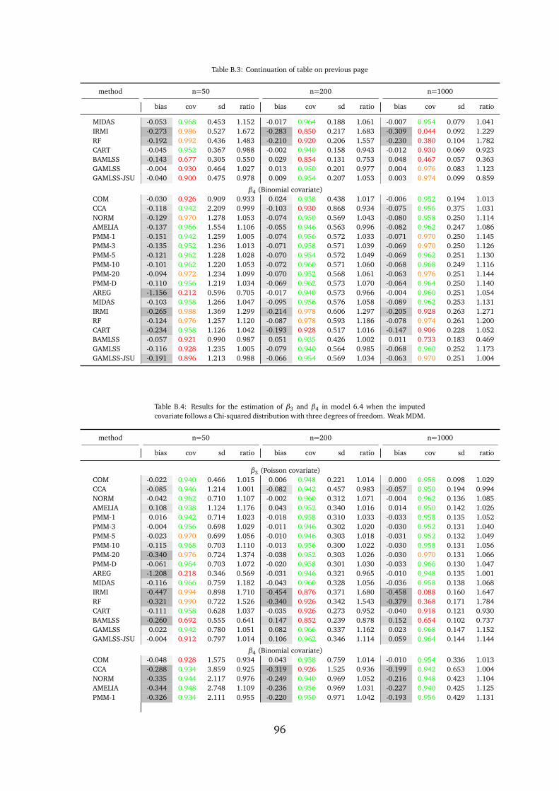
Table B.3: Continuation of table on previous page

method n=50 n=200 n=1000

bias cov sd ratio bias cov sd ratio bias cov sd ratio

MIDAS -0.053 0.968 0.453 1.152 -0.017 0.964 0.188 1.061 -0.007 0.954 0.079 1.041IRMI -0.273 0.986 0.527 1.672 -0.283 0.850 0.217 1.683 -0.309 0.044 0.092 1.229RF -0.192 0.992 0.436 1.483 -0.210 0.920 0.206 1.557 -0.230 0.380 0.104 1.782CART -0.045 0.952 0.367 0.988 -0.002 0.940 0.158 0.943 -0.012 0.930 0.069 0.923BAMLSS -0.143 0.677 0.305 0.550 0.029 0.854 0.131 0.753 0.048 0.467 0.057 0.363GAMLSS -0.004 0.930 0.464 1.027 0.013 0.950 0.201 0.977 0.004 0.976 0.083 1.123GAMLSS-JSU -0.040 0.900 0.475 0.978 0.009 0.954 0.207 1.053 0.003 0.974 0.099 0.859

β4 (Binomial covariate)COM -0.030 0.926 0.909 0.933 0.024 0.958 0.438 1.017 -0.006 0.952 0.194 1.013CCA -0.118 0.942 2.209 0.999 -0.103 0.930 0.868 0.934 -0.075 0.956 0.375 1.031NORM -0.129 0.970 1.278 1.053 -0.074 0.950 0.569 1.043 -0.080 0.958 0.250 1.114AMELIA -0.137 0.966 1.554 1.106 -0.055 0.946 0.563 0.996 -0.082 0.962 0.247 1.086PMM-1 -0.151 0.942 1.259 1.005 -0.074 0.956 0.572 1.033 -0.071 0.970 0.250 1.145PMM-3 -0.135 0.952 1.236 1.013 -0.071 0.958 0.571 1.039 -0.069 0.970 0.250 1.126PMM-5 -0.121 0.962 1.228 1.028 -0.070 0.954 0.572 1.049 -0.069 0.962 0.251 1.130PMM-10 -0.101 0.962 1.220 1.053 -0.072 0.960 0.571 1.060 -0.068 0.968 0.249 1.116PMM-20 -0.094 0.972 1.234 1.099 -0.070 0.952 0.568 1.061 -0.063 0.976 0.251 1.144PMM-D -0.110 0.956 1.219 1.034 -0.069 0.962 0.573 1.070 -0.064 0.964 0.250 1.140AREG -1.156 0.212 0.596 0.705 -0.017 0.940 0.573 0.966 -0.004 0.960 0.251 1.054MIDAS -0.103 0.958 1.266 1.047 -0.095 0.956 0.576 1.058 -0.089 0.962 0.253 1.131IRMI -0.265 0.988 1.369 1.299 -0.214 0.978 0.606 1.297 -0.205 0.928 0.263 1.271RF -0.124 0.976 1.257 1.120 -0.087 0.978 0.593 1.186 -0.078 0.974 0.261 1.200CART -0.234 0.958 1.126 1.042 -0.193 0.928 0.517 1.016 -0.147 0.906 0.228 1.052BAMLSS -0.057 0.921 0.990 0.987 0.051 0.935 0.426 1.002 0.011 0.733 0.183 0.469GAMLSS -0.116 0.928 1.235 1.005 -0.079 0.940 0.564 0.985 -0.068 0.960 0.252 1.173GAMLSS-JSU -0.191 0.896 1.213 0.988 -0.066 0.954 0.569 1.034 -0.063 0.970 0.251 1.004

Table B.4: Results for the estimation of β3 and β4 in model 6.4 when the imputedcovariate follows a Chi-squared distribution with three degrees of freedom. Weak MDM.

method n=50 n=200 n=1000

bias cov sd ratio bias cov sd ratio bias cov sd ratio

β3 (Poisson covariate)COM -0.022 0.940 0.466 1.015 0.006 0.948 0.221 1.014 0.000 0.958 0.098 1.029CCA -0.085 0.946 1.214 1.001 -0.082 0.942 0.457 0.983 -0.057 0.950 0.194 0.994NORM -0.042 0.962 0.710 1.107 -0.002 0.960 0.312 1.071 -0.004 0.962 0.136 1.085AMELIA 0.108 0.938 1.124 1.176 0.043 0.952 0.340 1.016 0.014 0.950 0.142 1.026PMM-1 0.016 0.942 0.714 1.023 -0.018 0.958 0.310 1.033 -0.033 0.958 0.135 1.052PMM-3 -0.004 0.956 0.698 1.029 -0.011 0.946 0.302 1.020 -0.030 0.952 0.131 1.040PMM-5 -0.023 0.970 0.699 1.056 -0.010 0.946 0.303 1.018 -0.031 0.952 0.132 1.049PMM-10 -0.115 0.968 0.703 1.110 -0.013 0.956 0.300 1.022 -0.030 0.958 0.131 1.056PMM-20 -0.340 0.976 0.724 1.374 -0.038 0.952 0.303 1.026 -0.030 0.970 0.131 1.066PMM-D -0.061 0.964 0.703 1.072 -0.020 0.958 0.301 1.030 -0.033 0.966 0.130 1.047AREG -1.208 0.218 0.346 0.569 -0.031 0.946 0.321 0.965 -0.010 0.948 0.135 1.001MIDAS -0.116 0.966 0.759 1.182 -0.043 0.960 0.328 1.056 -0.036 0.958 0.138 1.068IRMI -0.447 0.994 0.898 1.710 -0.454 0.876 0.371 1.680 -0.458 0.088 0.160 1.647RF -0.321 0.990 0.722 1.526 -0.340 0.926 0.342 1.543 -0.379 0.368 0.171 1.784CART -0.111 0.958 0.628 1.037 -0.035 0.926 0.273 0.952 -0.040 0.918 0.121 0.930BAMLSS -0.260 0.692 0.555 0.641 0.147 0.852 0.239 0.878 0.152 0.654 0.102 0.737GAMLSS 0.022 0.942 0.780 1.051 0.082 0.966 0.337 1.162 0.023 0.968 0.147 1.152GAMLSS-JSU -0.004 0.912 0.797 1.014 0.106 0.962 0.346 1.114 0.059 0.964 0.144 1.144

β4 (Binomial covariate)COM -0.048 0.928 1.575 0.934 0.043 0.958 0.759 1.014 -0.010 0.954 0.336 1.013CCA -0.288 0.934 3.859 0.925 -0.319 0.926 1.525 0.936 -0.199 0.942 0.653 1.004NORM -0.335 0.944 2.117 0.976 -0.249 0.940 0.969 1.052 -0.216 0.948 0.423 1.104AMELIA -0.344 0.948 2.748 1.109 -0.236 0.956 0.969 1.031 -0.227 0.940 0.425 1.125PMM-1 -0.326 0.934 2.111 0.955 -0.220 0.950 0.971 1.042 -0.193 0.956 0.429 1.131

96

Table B.4: Continuation of table on previous page

method n=50 n=200 n=1000

bias cov sd ratio bias cov sd ratio bias cov sd ratio

PMM-3 -0.320 0.954 2.072 0.961 -0.216 0.948 0.973 1.058 -0.200 0.950 0.428 1.117PMM-5 -0.265 0.946 2.078 0.987 -0.223 0.964 0.974 1.068 -0.197 0.940 0.427 1.117PMM-10 -0.233 0.956 2.071 1.020 -0.217 0.954 0.975 1.063 -0.195 0.954 0.428 1.130PMM-20 -0.246 0.970 2.100 1.091 -0.214 0.956 0.979 1.081 -0.192 0.954 0.427 1.138PMM-D -0.234 0.962 2.074 0.999 -0.219 0.948 0.970 1.061 -0.188 0.956 0.426 1.126AREG -3.071 0.230 1.026 0.539 -0.105 0.956 0.966 1.006 -0.068 0.962 0.418 1.069MIDAS -0.244 0.956 2.130 1.012 -0.227 0.956 0.987 1.073 -0.207 0.950 0.429 1.117IRMI -0.664 0.976 2.332 1.246 -0.622 0.956 1.036 1.294 -0.599 0.790 0.451 1.283RF -0.371 0.974 2.108 1.083 -0.287 0.962 0.997 1.143 -0.246 0.958 0.442 1.185CART -0.593 0.950 1.897 0.991 -0.480 0.916 0.885 0.991 -0.347 0.864 0.393 1.032BAMLSS -0.494 0.918 1.677 1.018 0.105 0.934 0.757 0.948 0.067 0.925 0.332 0.938GAMLSS -0.314 0.928 2.085 0.952 -0.192 0.948 0.972 1.053 -0.201 0.952 0.429 1.144GAMLSS-JSU -0.420 0.896 2.084 0.930 -0.143 0.956 0.969 1.037 -0.147 0.958 0.426 1.121

Table B.5: Results for the estimation of β3 and β4 in model 6.4. The imputed covariatex2 follows a Normal distribution. Strong non-monotone MDM.

method n=50 n=200 n=1000

bias cov sd ratio bias cov sd ratio bias cov sd ratio

β3 (Poisson covariate)COM -0.012 0.942 0.254 1.017 0.003 0.950 0.121 1.011 0.000 0.954 0.053 1.033CCA -0.288 0.888 0.445 1.004 -0.295 0.624 0.188 0.944 -0.295 0.058 0.081 0.953NORM -0.050 0.952 0.443 1.046 0.017 0.936 0.197 1.019 0.021 0.968 0.085 1.043PMM-1 0.005 0.914 0.461 0.987 0.006 0.928 0.205 0.972 -0.003 0.944 0.087 0.991PMM-3 -0.046 0.942 0.443 0.995 -0.002 0.926 0.190 0.928 -0.006 0.928 0.080 0.947PMM-5 -0.069 0.944 0.438 1.032 -0.011 0.930 0.189 0.955 -0.008 0.922 0.079 0.931PMM-10 -0.135 0.964 0.434 1.124 -0.029 0.926 0.184 0.952 -0.012 0.940 0.077 0.915PMM-20 -0.251 0.978 0.433 1.435 -0.069 0.938 0.184 1.022 -0.020 0.932 0.077 0.912PMM-D -0.098 0.960 0.437 1.086 -0.044 0.920 0.183 0.982 -0.029 0.906 0.076 0.892MIDAS -0.162 0.970 0.490 1.276 -0.055 0.950 0.219 1.064 -0.025 0.956 0.094 1.058RF -0.268 0.978 0.433 1.622 -0.256 0.868 0.202 1.563 -0.277 0.136 0.100 1.746CART -0.164 0.966 0.397 1.103 -0.055 0.904 0.173 0.886 -0.035 0.924 0.082 0.913GAMLSS -0.422 0.454 0.343 0.668 -0.089 0.832 0.220 0.661 -0.028 0.954 0.097 1.133GAMLSS-JSU -0.623 0.220 0.237 0.620 -0.189 0.762 0.212 0.574 -0.049 0.952 0.095 1.106

β4 (Binomial covariate)COM -0.028 0.926 0.857 0.936 0.023 0.958 0.413 1.015 -0.005 0.952 0.183 1.012CCA -0.940 0.876 1.438 0.961 -0.937 0.668 0.612 0.995 -0.970 0.070 0.266 0.953NORM -0.189 0.950 1.197 1.045 -0.091 0.952 0.544 1.058 -0.102 0.956 0.235 1.103PMM-1 -0.059 0.938 1.210 0.983 0.000 0.936 0.556 0.976 -0.016 0.962 0.240 1.065PMM-3 -0.028 0.948 1.178 1.004 -0.001 0.952 0.551 0.976 -0.014 0.960 0.238 1.052PMM-5 -0.012 0.940 1.164 1.006 0.003 0.946 0.546 0.986 -0.016 0.968 0.239 1.070PMM-10 0.008 0.954 1.163 1.038 0.014 0.954 0.540 0.996 -0.015 0.958 0.237 1.050PMM-20 -0.038 0.958 1.176 1.094 0.013 0.958 0.545 1.041 -0.014 0.972 0.238 1.059PMM-D 0.003 0.944 1.160 1.002 0.012 0.958 0.543 1.015 -0.014 0.966 0.236 1.068MIDAS -0.101 0.964 1.222 1.056 -0.026 0.958 0.562 1.040 -0.020 0.972 0.243 1.072RF -0.152 0.974 1.192 1.132 -0.088 0.978 0.570 1.193 -0.040 0.992 0.255 1.202CART -0.237 0.964 1.107 1.047 -0.246 0.906 0.511 0.986 -0.163 0.890 0.240 0.978GAMLSS -1.382 0.460 0.823 0.586 -0.331 0.822 0.507 0.519 -0.035 0.970 0.236 1.069GAMLSS-JSU -1.995 0.218 0.574 0.520 -0.510 0.742 0.486 0.426 -0.025 0.968 0.236 1.074

97

Table B.6: Results for the estimation of β3 and β4 in model 6.4. The imputed co-variate x2 follows a Student’s t distribution with three degrees of freedom. Strongnon-monotone MDM.

method n=50 n=200 n=1000

bias cov sd ratio bias cov sd ratio bias cov sd ratio

β3 (Poisson covariate)COM -0.012 0.944 0.269 1.017 0.002 0.948 0.128 1.011 -0.000 0.952 0.056 1.030CCA -0.369 0.852 0.475 0.944 -0.380 0.530 0.201 0.928 -0.375 0.016 0.086 0.933NORM -0.055 0.938 0.484 1.027 0.014 0.942 0.204 0.943 0.016 0.948 0.089 0.983PMM-1 0.024 0.908 0.511 0.929 0.022 0.918 0.216 0.957 0.008 0.936 0.090 0.955PMM-3 -0.019 0.936 0.482 0.964 0.011 0.910 0.199 0.910 0.011 0.924 0.083 0.904PMM-5 -0.068 0.946 0.482 0.993 0.003 0.912 0.195 0.916 0.010 0.916 0.081 0.884PMM-10 -0.148 0.972 0.480 1.105 -0.019 0.932 0.194 0.958 0.008 0.914 0.080 0.885PMM-20 -0.310 0.968 0.484 1.361 -0.081 0.936 0.198 1.029 -0.002 0.914 0.079 0.877PMM-D -0.103 0.956 0.482 1.053 -0.047 0.936 0.195 0.984 -0.014 0.916 0.080 0.879MIDAS -0.167 0.972 0.550 1.230 -0.056 0.958 0.234 1.048 -0.017 0.962 0.098 1.059RF -0.321 0.974 0.486 1.585 -0.302 0.828 0.222 1.629 -0.329 0.100 0.114 1.822CART -0.183 0.944 0.440 1.049 -0.039 0.924 0.183 0.890 -0.020 0.902 0.084 0.878GAMLSS -0.647 0.316 0.327 0.636 -0.259 0.686 0.226 0.479 -0.089 0.898 0.112 0.429GAMLSS-JSU -0.832 0.130 0.201 0.580 -0.489 0.478 0.199 0.409 -0.219 0.790 0.157 0.426

β4 (Binomial covariate)COM -0.030 0.926 0.909 0.933 0.024 0.958 0.438 1.017 -0.006 0.952 0.194 1.013CCA -0.616 0.922 1.417 0.960 -0.569 0.852 0.610 1.014 -0.596 0.388 0.265 0.937NORM -0.165 0.950 1.269 1.017 -0.061 0.936 0.574 1.006 -0.083 0.958 0.252 1.094PMM-1 -0.045 0.932 1.285 0.924 0.010 0.936 0.599 0.983 -0.011 0.966 0.259 1.070PMM-3 -0.010 0.944 1.261 0.939 0.015 0.938 0.585 0.973 -0.008 0.950 0.255 1.034PMM-5 -0.009 0.946 1.264 0.967 0.014 0.934 0.583 0.989 -0.005 0.960 0.256 1.044PMM-10 0.021 0.952 1.268 1.018 0.011 0.944 0.590 1.000 -0.005 0.960 0.255 1.031PMM-20 -0.006 0.960 1.276 1.067 0.023 0.942 0.588 1.029 -0.009 0.950 0.255 1.040PMM-D 0.007 0.950 1.265 0.993 0.025 0.938 0.588 1.018 0.001 0.960 0.255 1.064MIDAS -0.078 0.968 1.329 1.090 -0.030 0.950 0.602 1.043 -0.042 0.954 0.262 1.044RF -0.061 0.974 1.309 1.110 -0.020 0.970 0.614 1.158 -0.002 0.976 0.274 1.199CART -0.148 0.970 1.209 1.052 -0.170 0.950 0.551 1.050 -0.132 0.942 0.253 1.047GAMLSS -1.001 0.312 0.716 0.697 -0.411 0.670 0.495 0.576 -0.136 0.888 0.249 0.548GAMLSS-JSU -1.326 0.132 0.454 0.714 -0.710 0.472 0.430 0.485 -0.291 0.804 0.311 0.503

Table B.7: Results for the estimation of β3 and β4 in model 6.4. The imputed co-variate x2 follows a Chi-squared distribution with three degrees of freedom. Strongnon-monotone MDM.

method n=50 n=200 n=1000

bias cov sd ratio bias cov sd ratio bias cov sd ratio

β3 (Poisson covariate)COM -0.022 0.940 0.466 1.015 0.006 0.948 0.221 1.014 0.000 0.958 0.098 1.029CCA -0.585 0.880 0.812 0.981 -0.589 0.592 0.342 0.942 -0.589 0.024 0.146 0.949NORM -0.093 0.952 0.849 1.073 0.026 0.928 0.370 0.997 0.037 0.936 0.157 0.978PMM-1 -0.009 0.930 0.879 1.009 -0.017 0.932 0.397 0.988 -0.056 0.944 0.174 1.017PMM-3 -0.071 0.940 0.827 1.018 -0.018 0.916 0.365 0.949 -0.051 0.926 0.158 0.963PMM-5 -0.115 0.958 0.819 1.066 -0.023 0.928 0.359 0.956 -0.049 0.932 0.154 0.931PMM-10 -0.227 0.976 0.806 1.125 -0.037 0.934 0.348 0.959 -0.044 0.920 0.149 0.905PMM-20 -0.474 0.970 0.801 1.405 -0.110 0.950 0.346 1.012 -0.049 0.932 0.146 0.921PMM-D -0.168 0.970 0.818 1.098 -0.068 0.938 0.345 0.971 -0.058 0.920 0.144 0.903MIDAS -0.318 0.976 0.903 1.272 -0.133 0.952 0.416 1.092 -0.078 0.958 0.181 1.085RF -0.504 0.976 0.799 1.615 -0.482 0.858 0.374 1.529 -0.531 0.124 0.186 1.816CART -0.288 0.954 0.742 1.109 -0.089 0.910 0.325 0.895 -0.060 0.902 0.154 0.909GAMLSS -0.826 0.436 0.650 0.698 -0.187 0.744 0.403 0.535 0.026 0.958 0.185 0.913GAMLSS-JSU -1.187 0.216 0.457 0.629 -0.218 0.734 0.412 0.532 0.086 0.934 0.183 0.978

β4 (Binomial covariate)COM -0.048 0.928 1.575 0.934 0.043 0.958 0.759 1.014 -0.010 0.954 0.336 1.013CCA -1.616 0.888 2.568 0.962 -1.610 0.666 1.091 0.969 -1.626 0.090 0.473 0.951

98

Table B.7: Continuation of table on previous page

method n=50 n=200 n=1000

bias cov sd ratio bias cov sd ratio bias cov sd ratio

NORM -0.398 0.942 2.203 1.009 -0.211 0.948 0.995 1.055 -0.218 0.930 0.436 1.087PMM-1 -0.196 0.924 2.243 0.953 -0.098 0.938 1.046 0.992 -0.075 0.978 0.451 1.079PMM-3 -0.087 0.938 2.189 0.962 -0.052 0.938 1.029 1.008 -0.071 0.964 0.447 1.071PMM-5 -0.035 0.934 2.165 0.972 -0.063 0.946 1.020 0.997 -0.072 0.960 0.446 1.068PMM-10 0.025 0.944 2.160 0.997 -0.027 0.946 1.005 1.017 -0.065 0.972 0.445 1.058PMM-20 -0.051 0.964 2.163 1.044 0.003 0.956 1.011 1.053 -0.057 0.970 0.445 1.087PMM-D 0.007 0.944 2.166 0.998 -0.006 0.950 1.016 1.034 -0.047 0.968 0.445 1.089MIDAS -0.224 0.962 2.284 1.070 -0.135 0.948 1.058 1.059 -0.085 0.968 0.452 1.070RF -0.264 0.976 2.194 1.098 -0.184 0.972 1.046 1.180 -0.094 0.988 0.468 1.207CART -0.407 0.960 2.045 1.021 -0.446 0.934 0.960 1.027 -0.322 0.868 0.448 0.978GAMLSS -2.288 0.428 1.493 0.620 -0.843 0.758 0.910 0.500 -0.119 0.960 0.446 0.874GAMLSS-JSU -3.122 0.214 1.054 0.543 -0.847 0.736 0.910 0.478 0.010 0.960 0.447 0.982

Table B.8: Results for the estimation of β2, β3 and β4 in model 6.4. The imputedcovariate x2 follows a Normal distribution. Weak non-monotone MDM.

method n=50 n=200 n=1000

bias cov sd ratio bias cov sd ratio bias cov sd ratio

β2 (Normal covariate)COM -0.021 0.944 0.439 1.002 0.007 0.944 0.210 0.989 -0.007 0.952 0.093 1.005CCA -0.105 0.928 1.137 0.979 -0.094 0.924 0.420 0.941 -0.084 0.930 0.179 1.010NORM -0.112 0.970 0.709 1.140 -0.022 0.968 0.300 1.074 -0.016 0.952 0.131 1.057AMELIA 0.079 0.954 0.975 1.102 0.029 0.938 0.304 0.974 0.004 0.944 0.130 0.982PMM-1 0.037 0.946 0.730 0.991 0.008 0.926 0.300 0.963 -0.008 0.950 0.130 0.977PMM-3 0.002 0.948 0.706 1.006 0.003 0.938 0.295 0.954 -0.009 0.942 0.126 0.961PMM-5 -0.029 0.950 0.686 1.028 0.003 0.934 0.291 0.954 -0.009 0.944 0.125 0.940PMM-10 -0.099 0.966 0.671 1.069 -0.014 0.940 0.292 0.962 -0.010 0.940 0.124 0.949PMM-20 -0.294 0.976 0.673 1.282 -0.045 0.946 0.292 0.990 -0.014 0.944 0.124 0.955PMM-D -0.056 0.968 0.693 1.058 -0.029 0.954 0.293 0.985 -0.020 0.940 0.123 0.953AREG -1.201 0.216 0.325 0.516 -0.033 0.950 0.298 0.943 -0.016 0.934 0.125 0.969MIDAS -0.175 0.962 0.736 1.152 -0.053 0.956 0.315 1.005 -0.021 0.956 0.132 0.998IRMI -0.549 0.980 0.830 1.722 -0.591 0.694 0.354 1.715 -0.615 0.002 0.153 1.700RF -0.345 0.980 0.684 1.506 -0.365 0.902 0.328 1.594 -0.405 0.258 0.164 1.722CART -0.118 0.966 0.622 1.043 -0.040 0.916 0.276 0.904 -0.027 0.926 0.119 0.894GAMLSS -0.628 0.552 0.614 0.675 -0.022 0.886 0.314 0.626 0.021 0.954 0.134 1.030GAMLSS-JSU -0.928 0.370 0.510 0.600 -0.028 0.898 0.326 0.686 0.029 0.946 0.133 1.001

β3 (Poisson covariate)COM -0.012 0.942 0.254 1.017 0.003 0.950 0.121 1.011 0.000 0.954 0.053 1.033CCA -0.020 0.944 0.672 0.941 -0.031 0.948 0.249 0.991 -0.019 0.958 0.106 1.012NORM -0.043 0.976 0.422 1.175 0.000 0.964 0.178 1.099 0.005 0.962 0.077 1.091AMELIA 0.041 0.962 0.606 1.168 0.029 0.950 0.183 1.031 0.014 0.956 0.078 1.081PMM-1 0.009 0.938 0.443 0.998 0.003 0.938 0.176 0.968 0.003 0.954 0.077 1.048PMM-3 -0.003 0.962 0.426 1.024 0.004 0.928 0.172 0.953 0.002 0.966 0.074 1.034PMM-5 -0.016 0.964 0.411 1.054 0.001 0.936 0.170 0.944 0.001 0.960 0.074 1.022PMM-10 -0.058 0.974 0.400 1.142 0.001 0.942 0.168 0.978 -0.002 0.954 0.073 1.026PMM-20 -0.175 0.986 0.398 1.373 -0.017 0.952 0.170 1.010 -0.004 0.952 0.073 1.017PMM-D -0.031 0.968 0.406 1.083 -0.005 0.954 0.169 0.978 -0.006 0.956 0.073 1.025AREG -0.643 0.214 0.181 0.543 -0.015 0.934 0.175 0.953 -0.003 0.956 0.074 1.017MIDAS -0.097 0.974 0.434 1.201 -0.027 0.942 0.183 1.021 -0.007 0.962 0.077 1.055IRMI -0.226 0.990 0.480 1.747 -0.223 0.910 0.201 1.672 -0.227 0.138 0.087 1.708RF -0.190 0.994 0.402 1.594 -0.182 0.930 0.188 1.532 -0.198 0.414 0.093 1.723CART -0.107 0.976 0.370 1.118 -0.042 0.950 0.161 0.970 -0.025 0.950 0.071 0.969GAMLSS -0.364 0.554 0.356 0.704 -0.034 0.888 0.187 0.685 -0.006 0.964 0.081 1.073GAMLSS-JSU -0.504 0.366 0.298 0.645 -0.039 0.914 0.193 0.741 -0.013 0.974 0.081 1.088

β4 (Binomial covariate)COM -0.028 0.926 0.857 0.936 0.023 0.958 0.413 1.015 -0.005 0.952 0.183 1.012CCA -0.120 0.944 2.110 1.004 -0.134 0.936 0.834 0.936 -0.098 0.952 0.358 1.014

99

Table B.8: Continuation of table on previous page

method n=50 n=200 n=1000

bias cov sd ratio bias cov sd ratio bias cov sd ratio

NORM -0.120 0.962 1.181 1.043 -0.081 0.948 0.526 1.060 -0.078 0.962 0.229 1.123AMELIA -0.168 0.958 1.444 1.115 -0.126 0.952 0.525 1.038 -0.135 0.944 0.229 1.094PMM-1 -0.038 0.944 1.183 0.939 0.002 0.940 0.531 0.983 -0.004 0.962 0.230 1.072PMM-3 -0.052 0.946 1.162 0.966 -0.001 0.946 0.527 0.992 -0.005 0.964 0.231 1.062PMM-5 -0.044 0.944 1.148 0.968 -0.009 0.952 0.528 0.999 -0.005 0.974 0.232 1.082PMM-10 -0.050 0.952 1.137 1.003 -0.004 0.950 0.525 1.005 -0.005 0.970 0.229 1.075PMM-20 -0.106 0.970 1.144 1.079 -0.022 0.948 0.527 1.021 -0.008 0.964 0.231 1.084PMM-D -0.052 0.950 1.143 0.981 -0.013 0.958 0.525 1.018 -0.008 0.964 0.230 1.072AREG -1.936 0.214 0.542 0.466 -0.034 0.954 0.527 0.973 -0.016 0.962 0.230 1.065MIDAS -0.137 0.960 1.180 1.043 -0.044 0.946 0.535 1.017 -0.022 0.966 0.232 1.063IRMI -0.418 0.976 1.266 1.251 -0.381 0.964 0.571 1.348 -0.368 0.728 0.247 1.324RF -0.258 0.980 1.172 1.156 -0.178 0.964 0.553 1.205 -0.138 0.952 0.244 1.205CART -0.329 0.956 1.059 1.025 -0.232 0.918 0.496 0.979 -0.129 0.922 0.221 1.002GAMLSS -1.079 0.538 0.880 0.576 -0.154 0.878 0.502 0.614 -0.007 0.968 0.229 1.063GAMLSS-JSU -1.574 0.352 0.725 0.518 -0.135 0.886 0.513 0.647 -0.006 0.960 0.230 1.063

Table B.9: Results for the estimation of β2, β3 and β4 in model 6.4. The imputedcovariate x2 follows a Student’s t distribution with three degrees of freedom. Weaknon-monotone MDM.

method n=50 n=200 n=1000

bias cov sd ratio bias cov sd ratio bias cov sd ratio

β2 (t covariate)COM -0.012 0.944 0.302 0.990 0.005 0.948 0.136 0.982 -0.003 0.956 0.058 1.007CCA -0.064 0.940 0.878 1.001 -0.050 0.946 0.292 0.953 -0.048 0.934 0.115 1.034NORM -0.076 0.962 0.533 1.081 -0.002 0.944 0.203 0.942 -0.009 0.934 0.083 0.865AMELIA 0.029 0.950 0.789 1.163 0.030 0.946 0.213 0.898 0.003 0.920 0.084 0.853PMM-1 -0.002 0.932 0.558 0.978 0.021 0.940 0.202 0.905 0.008 0.928 0.082 0.891PMM-3 -0.014 0.946 0.534 1.023 0.016 0.928 0.200 0.926 0.007 0.924 0.082 0.917PMM-5 -0.029 0.956 0.520 1.031 0.011 0.940 0.201 0.951 0.005 0.926 0.081 0.900PMM-10 -0.064 0.962 0.511 1.081 0.008 0.956 0.202 0.974 0.003 0.930 0.081 0.922PMM-20 -0.151 0.974 0.498 1.183 -0.010 0.962 0.204 1.012 -0.001 0.936 0.081 0.945PMM-D -0.048 0.960 0.511 1.057 0.000 0.948 0.203 0.980 -0.002 0.934 0.082 0.969AREG -0.791 0.218 0.238 0.532 -0.037 0.940 0.209 0.920 -0.022 0.944 0.086 0.983MIDAS -0.144 0.962 0.558 1.193 -0.029 0.962 0.221 1.015 -0.008 0.942 0.088 0.982IRMI -0.372 0.968 0.612 1.724 -0.396 0.670 0.243 1.688 -0.409 0.002 0.099 1.621RF -0.220 0.980 0.512 1.482 -0.237 0.924 0.238 1.604 -0.282 0.252 0.114 1.784CART -0.085 0.954 0.462 1.018 -0.036 0.924 0.192 0.922 -0.040 0.922 0.086 0.901GAMLSS -0.584 0.404 0.387 0.656 -0.176 0.764 0.209 0.447 -0.067 0.906 0.101 0.402GAMLSS-JSU -0.768 0.216 0.276 0.555 -0.355 0.602 0.198 0.374 -0.196 0.796 0.099 0.261

β3 (Poisson covariate)COM -0.012 0.944 0.269 1.017 0.002 0.948 0.128 1.011 -0.000 0.952 0.056 1.030CCA -0.021 0.946 0.706 0.977 -0.039 0.942 0.263 0.986 -0.023 0.952 0.112 0.995NORM -0.032 0.948 0.450 1.122 0.003 0.962 0.188 1.049 0.003 0.952 0.081 1.035AMELIA 0.097 0.958 0.651 1.210 0.039 0.940 0.190 1.027 0.017 0.942 0.082 1.037PMM-1 0.061 0.930 0.466 0.973 0.018 0.938 0.186 0.990 0.012 0.944 0.079 0.999PMM-3 0.038 0.944 0.444 0.995 0.018 0.942 0.180 0.984 0.014 0.922 0.076 0.982PMM-5 0.018 0.956 0.437 1.001 0.017 0.944 0.176 0.976 0.015 0.930 0.076 0.986PMM-10 -0.051 0.964 0.428 1.060 0.013 0.946 0.178 1.006 0.015 0.918 0.075 0.982PMM-20 -0.196 0.970 0.427 1.251 -0.003 0.952 0.179 1.018 0.015 0.924 0.075 0.971PMM-D -0.010 0.954 0.428 1.021 0.008 0.942 0.179 0.993 0.012 0.934 0.075 0.987AREG -0.760 0.216 0.195 0.497 -0.006 0.942 0.182 0.896 0.010 0.936 0.078 1.004MIDAS -0.092 0.966 0.471 1.155 -0.017 0.968 0.193 1.033 0.005 0.946 0.081 1.012IRMI -0.273 0.986 0.527 1.672 -0.283 0.850 0.217 1.683 -0.309 0.044 0.092 1.229RF -0.208 0.984 0.439 1.486 -0.212 0.918 0.205 1.552 -0.232 0.368 0.104 1.771CART -0.086 0.954 0.396 1.061 -0.018 0.946 0.167 0.958 -0.015 0.926 0.074 0.950GAMLSS -0.569 0.406 0.321 0.601 -0.166 0.762 0.193 0.443 -0.043 0.904 0.087 0.361

100

Table B.9: Continuation of table on previous page

method n=50 n=200 n=1000

bias cov sd ratio bias cov sd ratio bias cov sd ratio

GAMLSS-JSU -0.733 0.220 0.228 0.499 -0.343 0.598 0.181 0.369 -0.159 0.798 0.122 0.324

β4 (Binomial covariate)COM -0.030 0.926 0.909 0.933 0.024 0.958 0.438 1.017 -0.006 0.952 0.194 1.013CCA -0.118 0.942 2.209 0.999 -0.103 0.930 0.868 0.934 -0.075 0.956 0.375 1.031NORM -0.111 0.952 1.298 1.026 -0.043 0.954 0.570 1.023 -0.045 0.966 0.249 1.090AMELIA -0.137 0.966 1.554 1.106 -0.055 0.946 0.563 0.996 -0.082 0.962 0.247 1.086PMM-1 -0.076 0.938 1.302 0.934 0.009 0.946 0.574 0.983 0.005 0.958 0.251 1.045PMM-3 -0.062 0.950 1.264 0.966 0.010 0.944 0.571 0.961 0.005 0.960 0.250 1.055PMM-5 -0.039 0.962 1.245 0.987 0.004 0.938 0.571 0.975 0.006 0.956 0.249 1.056PMM-10 -0.056 0.964 1.232 1.015 0.005 0.950 0.572 1.001 0.004 0.970 0.251 1.056PMM-20 -0.061 0.968 1.234 1.085 -0.012 0.960 0.572 1.018 0.003 0.960 0.252 1.060PMM-D -0.043 0.960 1.237 1.002 -0.001 0.946 0.572 0.992 0.002 0.960 0.253 1.077AREG -1.156 0.212 0.596 0.705 -0.017 0.940 0.573 0.966 -0.004 0.960 0.251 1.054MIDAS -0.116 0.962 1.292 1.074 -0.050 0.954 0.578 1.017 -0.031 0.960 0.256 1.040IRMI -0.265 0.988 1.369 1.299 -0.214 0.978 0.606 1.297 -0.205 0.928 0.263 1.271RF -0.138 0.982 1.268 1.152 -0.088 0.972 0.594 1.182 -0.065 0.972 0.264 1.198CART -0.226 0.964 1.162 1.067 -0.159 0.942 0.537 1.041 -0.107 0.940 0.238 1.058GAMLSS -0.879 0.390 0.812 0.726 -0.298 0.740 0.509 0.622 -0.080 0.898 0.245 0.575GAMLSS-JSU -1.130 0.210 0.576 0.632 -0.543 0.600 0.461 0.531 -0.255 0.786 0.251 0.408

Table B.10: Results for the estimation of β2, β3 and β4 in model 6.4. The imputedcovariate x2 follows a Chi-squared distribution with three degrees of freedom. Weaknon-monotone MDM.

method n=50 n=200 n=1000

bias cov sd ratio bias cov sd ratio bias cov sd ratio

β2 (t covariate)COM -0.020 0.942 0.338 0.995 0.001 0.950 0.158 0.993 -0.006 0.944 0.069 0.995CCA 0.002 0.936 1.024 0.937 -0.001 0.940 0.359 0.925 -0.002 0.948 0.145 0.954NORM -0.040 0.976 0.605 1.140 0.017 0.954 0.243 1.049 0.020 0.962 0.103 1.044PMM-1 0.021 0.936 0.622 0.993 -0.011 0.934 0.241 0.951 -0.024 0.926 0.101 0.937PMM-3 -0.011 0.942 0.595 1.007 -0.014 0.948 0.233 0.924 -0.023 0.930 0.099 0.924PMM-5 -0.036 0.966 0.581 1.039 -0.017 0.948 0.234 0.955 -0.026 0.930 0.098 0.933PMM-10 -0.084 0.976 0.565 1.126 -0.024 0.952 0.235 0.998 -0.024 0.938 0.097 0.918PMM-20 -0.205 0.972 0.557 1.258 -0.042 0.960 0.234 1.013 -0.027 0.926 0.097 0.940PMM-D -0.058 0.954 0.570 1.059 -0.032 0.956 0.234 0.989 -0.031 0.928 0.098 0.952MIDAS -0.132 0.972 0.609 1.194 -0.051 0.962 0.250 1.037 -0.033 0.934 0.106 0.986RF -0.232 0.978 0.566 1.482 -0.247 0.916 0.260 1.546 -0.287 0.344 0.127 1.684CART -0.111 0.946 0.527 1.055 -0.043 0.924 0.215 0.942 -0.033 0.910 0.091 0.883GAMLSS -0.457 0.576 0.517 0.750 -0.133 0.863 0.263 0.662 -0.063 0.938 0.117 1.047GAMLSS-JSU -0.660 0.369 0.419 0.632 -0.121 0.912 0.277 0.838 -0.103 0.873 0.115 1.018

β3 (Poisson covariate)COM -0.022 0.940 0.466 1.015 0.006 0.948 0.221 1.014 0.000 0.958 0.098 1.029CCA -0.085 0.946 1.214 1.001 -0.082 0.942 0.457 0.983 -0.057 0.950 0.194 0.994NORM -0.063 0.964 0.772 1.118 -0.005 0.954 0.322 1.066 0.006 0.952 0.141 1.068PMM-1 0.041 0.926 0.811 0.971 -0.011 0.948 0.331 0.979 -0.025 0.958 0.143 1.020PMM-3 0.013 0.944 0.793 1.037 -0.009 0.940 0.321 0.971 -0.022 0.952 0.138 0.983PMM-5 0.002 0.944 0.757 1.039 -0.001 0.942 0.318 0.966 -0.021 0.952 0.137 0.982PMM-10 -0.093 0.972 0.741 1.115 -0.008 0.954 0.316 0.984 -0.021 0.954 0.138 1.005PMM-20 -0.313 0.984 0.725 1.320 -0.024 0.952 0.315 1.023 -0.018 0.944 0.136 0.997PMM-D -0.030 0.964 0.738 1.052 -0.015 0.950 0.314 0.979 -0.019 0.946 0.135 0.984MIDAS -0.192 0.974 0.801 1.167 -0.061 0.950 0.339 1.030 -0.033 0.956 0.145 1.032RF -0.348 0.988 0.739 1.544 -0.342 0.928 0.342 1.514 -0.376 0.406 0.173 1.704CART -0.169 0.962 0.677 1.109 -0.068 0.936 0.295 0.983 -0.046 0.922 0.128 0.922GAMLSS -0.614 0.568 0.653 0.687 -0.043 0.861 0.334 0.595 0.041 0.946 0.147 1.081GAMLSS-JSU -0.902 0.369 0.519 0.587 0.037 0.912 0.357 0.771 0.077 0.917 0.147 1.077

β4 (Binomial covariate)

101

Table B.10: Continuation of table on previous page

method n=50 n=200 n=1000

bias cov sd ratio bias cov sd ratio bias cov sd ratio

COM -0.048 0.928 1.575 0.934 0.043 0.958 0.759 1.014 -0.010 0.954 0.336 1.013CCA -0.288 0.934 3.859 0.925 -0.319 0.926 1.525 0.936 -0.199 0.942 0.653 1.004NORM -0.289 0.956 2.172 0.983 -0.162 0.948 0.968 1.036 -0.139 0.964 0.426 1.118PMM-1 -0.170 0.916 2.162 0.906 -0.019 0.950 0.973 0.994 -0.009 0.970 0.430 1.070PMM-3 -0.123 0.936 2.128 0.928 -0.010 0.948 0.974 0.992 -0.008 0.970 0.429 1.074PMM-5 -0.105 0.938 2.101 0.949 -0.025 0.952 0.975 1.006 -0.010 0.968 0.425 1.064PMM-10 -0.091 0.948 2.080 0.979 -0.046 0.946 0.974 1.001 -0.013 0.962 0.427 1.068PMM-20 -0.185 0.964 2.105 1.053 -0.051 0.954 0.971 1.020 -0.014 0.968 0.426 1.061PMM-D -0.109 0.942 2.097 0.969 -0.037 0.952 0.975 1.004 -0.015 0.960 0.425 1.076MIDAS -0.284 0.952 2.187 1.022 -0.134 0.956 0.988 0.996 -0.047 0.964 0.430 1.061RF -0.406 0.980 2.132 1.138 -0.309 0.974 1.006 1.192 -0.225 0.958 0.445 1.199CART -0.561 0.954 1.965 1.014 -0.405 0.930 0.914 1.023 -0.242 0.918 0.409 1.043GAMLSS -1.756 0.542 1.614 0.627 -0.400 0.859 0.920 0.614 -0.030 0.966 0.424 1.073GAMLSS-JSU -2.579 0.355 1.344 0.596 -0.175 0.906 0.950 0.751 0.018 0.970 0.424 1.075

102

Bibliography

Albert, James H. and Siddhartha Chib (June 1993). “Bayesian Analysis of Binary andPolychotomous Response Data”. In: Journal of the American Statistical Association88.422, pp. 669–679. ISSN: 0162-1459. DOI: 10.1080/01621459.1993.10476321.URL: http://www.tandfonline.com/doi/abs/10.1080/01621459.1993.10476321 (visited on 07/31/2017).

Alexander Kowarik and Matthias Templ (Oct. 2016). Imputation with the R PackageVIM | Kowarik | Journal of Statistical Software. URL: https://www.jstatsoft.org/article/view/v074i07 (visited on 04/11/2017).

Andridge, Rebecca R. and Roderick J. A. Little (2010). “A Review of Hot Deck Im-putation for Survey Non-response”. en. In: International Statistical Review 78.1,pp. 40–64. ISSN: 1751-5823. DOI: 10.1111/j.1751-5823.2010.00103.x. URL:http://onlinelibrary.wiley.com/doi/10.1111/j.1751-5823.2010.00103.

x/abstract (visited on 01/04/2015).Barnard, John and Donald B. Rubin (1999). “Small-Sample Degrees of Freedom with

Multiple Imputation”. In: Biometrika 86.4, pp. 948–955. ISSN: 0006-3444. URL:http://www.jstor.org/stable/2673599 (visited on 05/02/2017).

Beck, Aaron T. et al. (1996). “Comparison of Beck Depression Inventories-IA and-II inPsychiatric Outpatients”. In: Journal of Personality Assessment 67.3, 588–597. ISSN:1532-7752. DOI: 10.1207/s15327752jpa6703_13. URL: http://dx.doi.org/10.1207/s15327752jpa6703_13.

Buuren, S. Van et al. (Dec. 2006). “Fully conditional specification in multivariate im-putation”. In: Journal of Statistical Computation and Simulation 76.12, pp. 1049–1064. ISSN: 0094-9655. DOI: 10.1080/10629360600810434. URL: http://dx.doi.org/10.1080/10629360600810434 (visited on 07/31/2017).

Cameron, Colin A. and Pravin K. Trivedi (May 2005). Microeconometrics : methodsand applications. Cambridge University Press. ISBN: 0521848059. URL: http://www.amazon.com/exec/obidos/redirect?tag=citeulike07-20\&path=ASIN/

0521848059.Cantoni, Eva and Elvezio Ronchetti (2001). “Robust Inference for Generalized Linear

Models”. In: Journal of the American Statistical Association 96.455, pp. 1022–1030.ISSN: 01621459. URL: http://www.jstor.org/stable/2670248.

Carpenter, James and Michael Kenward (2012). Multiple Imputation and its Appli-cation. URL: http : / / www . wiley . com / WileyCDA / WileyTitle / productCd -

0470740523.html (visited on 04/10/2017).Cochran, W. G. (Apr. 1934). “The distribution of quadratic forms in a normal system,

with applications to the analysis of covariance”. In: Mathematical Proceedings of the

103

Cambridge Philosophical Society 30.2, pp. 178–191. ISSN: 1469-8064, 0305-0041.DOI: 10.1017/S0305004100016595.

Cox, D. R. (1958). “The Regression Analysis of Binary Sequences”. In: Journal ofthe Royal Statistical Society. Series B (Methodological) 20.2, pp. 215–242. ISSN:00359246. URL: http://www.jstor.org/stable/2983890.

Dahl, Fredrik A. (Aug. 2007). “Convergence of random k-nearest-neighbour imputa-tion”. In: Computational Statistics & Data Analysis 51.12, pp. 5913–5917. ISSN:01679473. DOI: 10.1016/j.csda.2006.11.007. URL: http://linkinghub.elsevier.com/retrieve/pii/S0167947306004270.

De Jong, Roel (2012). “Robust Multiple Imputation”. PhD thesis. Universität Hamburg.URL: http://ediss.sub.uni-hamburg.de/volltexte/2012/5971/.

De Jong, Roel, Stef van Buuren, and Martin Spiess (Mar. 2016). “Multiple Imputationof Predictor Variables Using Generalized Additive Models”. In: Communicationsin Statistics - Simulation and Computation 45.3, pp. 968–985. ISSN: 0361-0918.DOI: 10.1080/03610918.2014.911894. URL: http://dx.doi.org/10.1080/03610918.2014.911894 (visited on 05/15/2016).

Demirtas, Hakan, Sally A. Freels, and Recai M. Yucel (Feb. 2008). “Plausibility of mul-tivariate normality assumption when multiply imputing non-Gaussian continuousoutcomes: a simulation assessment”. In: Journal of Statistical Computation andSimulation 78.1, pp. 69–84. ISSN: 0094-9655. DOI: 10.1080/10629360600903866.URL: http://dx.doi.org/10.1080/10629360600903866 (visited on 07/31/2017).

Dempster, A. P., N. M. Laird, and D. B. Rubin (1977). “Maximum likelihood from in-complete data via the EM algorithm”. In: JOURNAL OF THE ROYAL STATISTICALSOCIETY, SERIES B 39.1, pp. 1–38.

Deng, Yi et al. (Feb. 2016). “Multiple Imputation for General Missing Data Patternsin the Presence of High-dimensional Data”. In: Scientific Reports 6. ISSN: 2045-2322. DOI: 10.1038/srep21689. URL: http://www.ncbi.nlm.nih.gov/pmc/articles/PMC4751511/ (visited on 05/16/2016).

Donneau, A. F. et al. (May 2015a). “A Simulation Study Comparing Multiple Imputa-tion Methods for Incomplete Longitudinal Ordinal Data”. In: Communications inStatistics - Simulation and Computation 44.5, pp. 1311–1338. ISSN: 0361-0918.DOI: 10.1080/03610918.2013.818690. URL: http://dx.doi.org/10.1080/03610918.2013.818690 (visited on 05/16/2016).

Donneau, A. F. et al. (May 2015b). “Simulation-Based Study Comparing Multiple Im-putation Methods for Non-Monotone Missing Ordinal Data in Longitudinal Set-tings”. In: Journal of Biopharmaceutical Statistics 25.3, pp. 570–601. ISSN: 1054-3406. DOI: 10.1080/10543406.2014.920864. URL: http://dx.doi.org/10.1080/10543406.2014.920864 (visited on 05/16/2016).

Doove, L. L., S. Van Buuren, and E. Dusseldorp (Apr. 2014). “Recursive partitioning formissing data imputation in the presence of interaction effects”. In: ComputationalStatistics & Data Analysis 72, pp. 92–104. ISSN: 0167-9473. DOI: 10.1016/j.csda.2013.10.025. URL: http://www.sciencedirect.com/science/article/pii/S0167947313003939 (visited on 07/19/2017).

Efron, B. (Jan. 1979). “Bootstrap Methods: Another Look at the Jackknife”. EN. In: TheAnnals of Statistics 7.1, pp. 1–26. ISSN: 0090-5364, 2168-8966. DOI: 10.1214/aos/1176344552. URL: http://projecteuclid.org/euclid.aos/1176344552.

104

Efron, Bradley (2012). “Bayesian inference and the parametric bootstrap”. In: TheAnnals of Applied Statistics 6.4, 1971–1997. ISSN: 1932-6157. DOI: 10.1214/12-aoas571. URL: http://dx.doi.org/10.1214/12-aoas571.

Eilers, Paul H. C., Brian D. Marx, and Maria Durbán (2015). “Twenty years of P-splines”. eng. In: SORT-Statistics and Operations Research Transactions 39.2, pp. 149–186. ISSN: 2013-8830. URL: http://www.raco.cat/index.php/SORT/article/view/302258 (visited on 11/10/2017).

Elashoff, Michael and Louise Ryan (2004). “An EM Algorithm for Estimating Equa-tions”. In: Journal of Computational and Graphical Statistics 13.1, pp. 48–65. ISSN:1061-8600. DOI: 10.2307/1391144. URL: http://www.jstor.org/stable/1391144 (visited on 08/30/2017).

Fushiki, Tadayoshi (2005). “Bootstrap prediction and Bayesian prediction under mis-specified models”. In: Bernoulli 11.4, 747–758. ISSN: 1350-7265. DOI: 10.3150/bj/1126126768. URL: http://dx.doi.org/10.3150/bj/1126126768.

Gaffert, Philipp, Florian Meinfelder, and Volker Bosch (Jan. 2016). “Towards an MI-proper Predictive Mean Matching”. English. URL: https://www.uni-bamberg.de/fileadmin/uni/fakultaeten/sowi_lehrstuehle/statistik/Personen/

Dateien_Florian/properPMM.pdf.Graham, John W. (2009). “Missing data analysis: making it work in the real world”.

eng. In: Annual Review of Psychology 60, pp. 549–576. ISSN: 0066-4308. DOI: 10.1146/annurev.psych.58.110405.085530.

Graham, John W., Patricio E. Cumsille, and Elvira Elek-Fisk (2003). “Methods for Han-dling Missing Data”. en. In: Handbook of Psychology. John Wiley & Sons, Inc. ISBN:978-0-471-26438-5. URL: http://onlinelibrary.wiley.com/doi/10.1002/0471264385.wei0204/abstract (visited on 05/14/2016).

Graham, John W., Allison E. Olchowski, and Tamika D. Gilreath (Sept. 2007). “Howmany imputations are really needed? Some practical clarifications of multiple im-putation theory”. eng. In: Prevention Science: The Official Journal of the Society forPrevention Research 8.3, pp. 206–213. ISSN: 1389-4986. DOI: 10.1007/s11121-007-0070-9.

Hamilton, Max (1964). “A Rating Scale for Depressive Disorders”. In: PsychologicalReports 14.3, 914–914. ISSN: 1558-691X. DOI: 10.2466/pr0.1964.14.3.914.URL: http://dx.doi.org/10.2466/pr0.1964.14.3.914.

Harrell, Frank E. (2015). Regression Modeling Strategies. 2nd Edition. Springer Seriesin Statistics. New York, NY: Springer New York. ISBN: 9783319194257. DOI: 10.1007/978-3-319-19425-7. URL: http://dx.doi.org/10.1007/978-3-319-19425-7 (visited on 05/10/2016).

Harris, Ian R. (1989). “Predictive Fit for Natural Exponential Families”. In: Biometrika76.4, pp. 675–684. ISSN: 0006-3444. DOI: 10.2307/2336627. URL: http://www.jstor.org/stable/2336627 (visited on 02/16/2017).

He, Yulei and Trivellore E. Raghunathan (Feb. 2009). “On the Performance of Se-quential Regression Multiple Imputation Methods with Non Normal Error Dis-tributions”. In: Communications in Statistics - Simulation and Computation 38.4,pp. 856–883. ISSN: 0361-0918. DOI: 10.1080/03610910802677191. URL: http://dx.doi.org/10.1080/03610910802677191 (visited on 07/08/2015).

105

Henderson, C. R. et al. (1959). “The Estimation of Environmental and Genetic Trendsfrom Records Subject to Culling”. In: Biometrics 15.2, p. 192. ISSN: 0006-341X.DOI: 10.2307/2527669. URL: http://dx.doi.org/10.2307/2527669.

Hippel, Paul T. von (Feb. 2013). “Should a Normal Imputation Model be Modified toImpute Skewed Variables?” en. In: Sociological Methods & Research 42.1, pp. 105–138. ISSN: 0049-1241, 1552-8294. DOI: 10.1177/0049124112464866. URL: http://smr.sagepub.com/content/42/1/105 (visited on 05/15/2016).

Honaker, James and Gary King (Apr. 2010). “What to Do about Missing Values inTime-Series Cross-Section Data”. en. In: American Journal of Political Science 54.2,pp. 561–581. ISSN: 1540-5907. DOI: 10.1111/j.1540-5907.2010.00447.x. URL:http://onlinelibrary.wiley.com/doi/10.1111/j.1540-5907.2010.00447.

x/abstract (visited on 07/18/2017).Honaker, James, Gary King, and Matthew Blackwell (2011). “Amelia II: A Program for

Missing Data”. In: Journal of Statistical Software 45.7, pp. 1–47. ISSN: 1548-7660.URL: http://www.jstatsoft.org/v45/i07.

Javaras, Kristin N. and David A. Van Dyk (Sept. 2003). “Multiple Imputation for Incom-plete Data With Semicontinuous Variables”. In: Journal of the American StatisticalAssociation 98.463, pp. 703–715. ISSN: 0162-1459. DOI: 10.1198/016214503000000611.(Visited on 05/10/2016).

Kropko, Jonathan et al. (Apr. 2014). “Multiple Imputation for Continuous and Cate-gorical Data: Comparing Joint Multivariate Normal and Conditional Approaches”.en. In: Political Analysis, mpu007. ISSN: 1047-1987, 1476-4989. DOI: 10.1093/pan/mpu007. URL: http://pan.oxfordjournals.org/content/early/2014/04/23/pan.mpu007 (visited on 05/16/2016).

Li, K. H., T. E. Raghunathan, and D. B. Rubin (1991). “Large-Sample Significance Lev-els from Multiply Imputed Data Using Moment-Based Statistics and an F ReferenceDistribution”. In: Journal of the American Statistical Association 86.416, pp. 1065–1073. ISSN: 0162-1459. DOI: 10.2307/2290525. URL: http://www.jstor.org/stable/2290525 (visited on 05/02/2017).

Little, Roderick J. A. (1988). “Missing-Data Adjustments in Large Surveys”. In: Journalof Business & Economic Statistics 6.3, pp. 287–296. ISSN: 07350015. DOI: 10.2307/1391881. URL: http://www.jstor.org/stable/1391881?origin=crossref.

Little, Roderick J. A. and Donald B. Rubin (Sept. 2002). Statistical Analysis with MissingData, 2nd Edition. English. 2nd Edition edition. Hoboken, N.J: Wiley-Blackwell.ISBN: 978-0-471-18386-0.

Liu, Jingchen et al. (Nov. 2013). “On the stationary distribution of iterative imputa-tions”. en. In: Biometrika, ast044. ISSN: 0006-3444, 1464-3510. DOI: 10.1093/biomet/ast044. URL: http://biomet.oxfordjournals.org/content/early/2013/11/21/biomet.ast044 (visited on 05/19/2016).

Louis, Thomas A. (1982). “Finding the Observed Information Matrix when Using theEM Algorithm”. In: Journal of the Royal Statistical Society. Series B (Methodological)44.2, pp. 226–233. ISSN: 0035-9246. URL: http://www.jstor.org/stable/2345828.

McCullagh, Peter and John A. Nelder (Aug. 1989). Generalized Linear Models, SecondEdition. URL: https://www.crcpress.com/Generalized- Linear- Models-Second-Edition/McCullagh-Nelder/p/book/9780412317606.

106

Meng, Xiao-Li (Nov. 1994). “Multiple-Imputation Inferences with Uncongenial Sourcesof Input”. EN. In: Statistical Science 9.4, pp. 538–558. ISSN: 0883-4237, 2168-8745.DOI: 10.1214/ss/1177010269. URL: http://projecteuclid.org/euclid.ss/1177010269 (visited on 01/04/2015).

Meng, Xiao-Li and Martin Romero (Dec. 2003). “Discussion: Efficiency and Self-efficiencyWith Multiple Imputation Inference”. en. In: International Statistical Review 71.3,pp. 607–618. ISSN: 1751-5823. DOI: 10.1111/j.1751-5823.2003.tb00215.x.URL: http://onlinelibrary.wiley.com/doi/10.1111/j.1751-5823.2003.tb00215.x/abstract (visited on 05/02/2017).

Morris, Tim P, Ian R White, and Patrick Royston (2014). “Tuning multiple imputationby predictive mean matching and local residual draws”. In: BMC Medical ResearchMethodology 14.1. ISSN: 1471-2288. DOI: 10.1186/1471-2288-14-75. URL: http://dx.doi.org/10.1186/1471-2288-14-75.

Nielsen, Søren Feodor (2003). “Proper and Improper Multiple Imputation”. en. In:International Statistical Review 71.3, pp. 593–607. ISSN: 1751-5823. DOI: 10.1111/j.1751-5823.2003.tb00214.x. URL: http://onlinelibrary.wiley.com/doi/10.1111/j.1751-5823.2003.tb00214.x/abstract (visited on 01/04/2015).

R Core Team (2017). R: A Language and Environment for Statistical Computing. RFoundation for Statistical Computing. Vienna, Austria. URL: https://www.R-project.org/.

Raghunathan, Trivellore E. et al. (2001). A multivariate technique for multiply imputingmissing values using a sequence of regression models. Survey Methodology 27.

Rigby, R. A. and D. M. Stasinopoulos (June 2005). “Generalized additive models forlocation, scale and shape”. en. In: Journal of the Royal Statistical Society: Series C(Applied Statistics) 54.3, pp. 507–554. ISSN: 1467-9876. DOI: 10.1111/j.1467-9876.2005.00510.x. URL: http://onlinelibrary.wiley.com/doi/10.1111/j.1467-9876.2005.00510.x/abstract (visited on 07/29/2014).

Robins, J. M. and N. Wang (Mar. 2000). “Inference for imputation estimators”. en.In: Biometrika 87.1, pp. 113–124. ISSN: 0006-3444, 1464-3510. DOI: 10.1093/biomet/87.1.113. URL: http://biomet.oxfordjournals.org/content/87/1/113 (visited on 01/04/2015).

Rubin, Donald B. (Dec. 1976). “Inference and missing data”. en. In: Biometrika 63.3,pp. 581–592. ISSN: 0006-3444, 1464-3510. DOI: 10.1093/biomet/63.3.581.URL: http://biomet.oxfordjournals.org/content/63/3/581 (visited on01/04/2015).

— (Jan. 1986). “Statistical Matching Using File Concatenation with Adjusted Weightsand Multiple Imputations”. In: Journal of Business & Economic Statistics 4.1, pp. 87–94. ISSN: 0735-0015. DOI: 10.2307/1391390. URL: http://www.jstor.org/stable/1391390 (visited on 01/04/2015).

— (1987). Multiple Imputation for Nonresponse in Surveys. en. John Wiley & Sons.ISBN: 978-0-471-65574-9.

— (June 1996). “Multiple Imputation After 18+ Years”. In: Journal of the Ameri-can Statistical Association 91.434, pp. 473–489. ISSN: 0162-1459. DOI: 10.2307/2291635. URL: http://www.jstor.org/stable/2291635 (visited on 01/04/2015).

— (2003). “Discussion on Multiple Imputation”. en. In: International Statistical Re-view 71.3, pp. 619–625. ISSN: 1751-5823. DOI: 10.1111/j.1751-5823.2003.

107

tb00216.x. URL: http://onlinelibrary.wiley.com/doi/10.1111/j.1751-5823.2003.tb00216.x/abstract (visited on 01/04/2015).

Salfran, Daniel, Pascal Jordan, and Martin Spiess (2016). Missing data: On criteria toevaluate imputation methods. Tech. rep. Discussion Paper.

Salfran, Daniel and Martin Spiess (2015). A Comparison of Multiple Imputation Tech-niques. Tech. rep. Discussion Paper.

— (2018a). “Generalized Additive Model Multiple Imputation by Chained EquationsWith Package ImputeRobust”. In: The R Journal, to appear.

— (2018b). ImputeRobust: Robust Multiple Imputation with Generalized Additive Mod-els for Location Scale and Shape. R package version 1.3.

SAS Institute Inc. (2015). SAS® Help Center: SAS/STAT 14.1 User’s Guide. Cary, NC:SAS Institute Inc. URL: http://documentation.sas.com/?docsetId=statug&docsetTarget=titlepage.htm&docsetVersion=14.2&locale=en (visited on07/18/2017).

Schafer, J. L. (Aug. 1997). Analysis of Incomplete Multivariate Data. en. CRC Press.ISBN: 978-1-4398-2186-2.

Schafer, Joseph L. and John W. Graham (June 2002). “Missing data: our view of thestate of the art”. eng. In: Psychological Methods 7.2, pp. 147–177. ISSN: 1082-989X.

Schenker, Nathaniel and J. M. G. Taylor (1996). “Partially parametric techniques formultiple imputation”. In: Computational Statistics & Data Analysis 22.4, pp. 425–446. ISSN: 01679473. DOI: 10.1016/0167-9473(95)00057-7. URL: http://www.sciencedirect.com/science/article/pii/0167947395000577.

Seal, Hilary L. (1967). “Studies in the History of Probability and Statistics. XV: TheHistorical Development of the Gauss Linear Model”. In: Biometrika 54.1/2, p. 1.ISSN: 0006-3444. DOI: 10.2307/2333849. URL: http://dx.doi.org/10.2307/2333849.

Shah, Anoop (2014). CALIBERrfimpute: Imputation in MICE using Random Forest. Rpackage version 0.1-6.

Siddique, Juned and Thomas R. Belin (Jan. 2008). “Multiple imputation using an iter-ative hot-deck with distance-based donor selection”. eng. In: Statistics in Medicine27.1, pp. 83–102. ISSN: 0277-6715. DOI: 10.1002/sim.3001.

Siddique, Juner and Ofer Harel (2009). “MIDAS: A SAS Macro for Multiple Impu-tation Using Distance-Aided Selection of Donors”. In: Journal of Statistical Soft-ware. URL: https://www.jstatsoft.org/article/view/v029i09 (visited on05/10/2016).

Stasinopoulos, D. M. and R. A. Rigby (2007). “Generalized Additive Models for Lo-cation Scale and Shape (GAMLSS) in R”. In: Journal of Statistical Software 23.7,pp. 1–46. ISSN: 1548-7660. URL: http://www.jstatsoft.org/v23/i07.

Templ, Matthias, Alexander Kowarik, and Peter Filzmoser (Oct. 2011). “Iterative step-wise regression imputation using standard and robust methods”. In: ComputationalStatistics & Data Analysis 55.10, pp. 2793–2806. ISSN: 0167-9473. DOI: 10.1016/j.csda.2011.04.012. URL: http://www.sciencedirect.com/science/

article/pii/S0167947311001411 (visited on 02/09/2015).Tutz, Gerhard and Shahla Ramzan (2014). Improved Methods for the Imputation of

Missing Data by Nearest Neighbor Methods. Tech. rep. 172. Department of Statistics:University of Munich.

108

Umlauf, Nikolaus, Nadja Klein, and Achim Zeileis (2017). “BAMLSS: Bayesian AdditiveModels for Location, Scale and Shape (and Beyond)”. In: Journal of Computationaland Graphical Statistics, 0–0. ISSN: 1537-2715. DOI: 10.1080/10618600.2017.1407325. URL: http://dx.doi.org/10.1080/10618600.2017.1407325.

Van Buuren, Stef (June 2007). “Multiple imputation of discrete and continuous databy fully conditional specification”. eng. In: Statistical Methods in Medical Research16.3, pp. 219–242. ISSN: 0962-2802. DOI: 10.1177/0962280206074463.

— (Mar. 2012). Flexible Imputation of Missing Data. CRC Press. (Visited on 05/10/2016).Van Buuren, Stef and Karin Groothuis-Oudshoorn (2011). “mice: Multivariate Imputa-

tion by Chained Equations in R”. In: Journal of Statistical Software 45.3, pp. 1–67.URL: http://www.jstatsoft.org/v45/i03/.

Vink, Gerko et al. (2014). “Predictive mean matching imputation of semicontinuousvariables”. en. In: Statistica Neerlandica 68.1, pp. 61–90. ISSN: 1467-9574. DOI:10.1111/stan.12023. URL: http://onlinelibrary.wiley.com/doi/10.1111/stan.12023/abstract (visited on 01/21/2015).

Wang, Naisyin and James M. Robins (Dec. 1998). “Large-sample theory for paramet-ric multiple imputation procedures”. en. In: Biometrika 85.4, pp. 935–948. ISSN:0006-3444, 1464-3510. DOI: 10.1093/biomet/85.4.935. URL: http://biomet.oxfordjournals.org/content/85/4/935 (visited on 05/14/2016).

Yang, S. and J. K. Kim (Mar. 2016). “A note on multiple imputation for method ofmoments estimation”. In: Biometrika 103.1, pp. 244–251. ISSN: 0006-3444. DOI:10.1093/biomet/asv073. URL: https://academic.oup.com/biomet/article-abstract/103/1/244/2390333/A- note- on- multiple- imputation- for-

method-of (visited on 06/09/2017).Yohai, Victor J. (June 1987). “High Breakdown-Point and High Efficiency Robust Es-

timates for Regression”. EN. In: The Annals of Statistics 15.2, pp. 642–656. ISSN:0090-5364, 2168-8966. DOI: 10.1214/aos/1176350366.

Yu, L.-M., Andrea Burton, and Oliver Rivero-Arias (June 2007). “Evaluation of soft-ware for multiple imputation of semi-continuous data”. en. In: Statistical Methodsin Medical Research 16.3, pp. 243–258. ISSN: 0962-2802, 1477-0334. DOI: 10.1177/0962280206074464. URL: http://smm.sagepub.com/content/16/3/243(visited on 01/04/2015).

109