
Multiple growth-correlated life history traits estimated ... · separate individual organisms...
72
Multiple growth-correlated life history traits estimated simultaneously in individuals Mollet, F., Ernande, B., Brunel, T. and Rijnsdorp, A.D. IIASA Interim Report June 2010
Transcript of Multiple growth-correlated life history traits estimated ... · separate individual organisms...

Multiple growth-correlated life history traits estimated simultaneously in individuals
Mollet, F., Ernande, B., Brunel, T. and Rijnsdorp, A.D.
IIASA Interim ReportJune 2010

Mollet, F., Ernande, B., Brunel, T. and Rijnsdorp, A.D. (2010) Multiple growth-correlated life history traits estimated
simultaneously in individuals. IIASA Interim Report . IIASA, Laxenburg, Austria, IR-10-050 Copyright © 2010 by the
author(s). http://pure.iiasa.ac.at/9433/
Interim Reports on work of the International Institute for Applied Systems Analysis receive only limited review. Views or
opinions expressed herein do not necessarily represent those of the Institute, its National Member Organizations, or other
organizations supporting the work. All rights reserved. Permission to make digital or hard copies of all or part of this work
for personal or classroom use is granted without fee provided that copies are not made or distributed for profit or commercial
advantage. All copies must bear this notice and the full citation on the first page. For other purposes, to republish, to post on
servers or to redistribute to lists, permission must be sought by contacting [email protected]

International Institute for Applied Systems Analysis Schlossplatz 1 A-2361 Laxenburg, Austria
Tel: +43 2236 807 342Fax: +43 2236 71313
E-mail: [email protected]: www.iiasa.ac.at
Interim Reports on work of the International Institute for Applied Systems Analysis receive onlylimited review. Views or opinions expressed herein do not necessarily represent those of theInstitute, its National Member Organizations, or other organizations supporting the work.
Interim Report IR-10-050
Multiple growth-correlated life history traits estimated simultaneously in individuals Fabian Mollet ([email protected]) Bruno Ernande ([email protected]) Thomas Brunel ([email protected]) Adriaan D. Rijnsdorp ([email protected])
Approved by
Ulf Dieckmann Leader, Evolution and Ecology Program
June 2010

Contents
Abstract .............................................................................................................................2
1. Introduction...................................................................................................................3
2. Material and methods....................................................................................................6
2.1 Parameter estimation.............................................................................................6
2.1.1 Energy allocation model ..............................................................................6
2.1.2 Fitting procedure…………………………………………………………..9
2.1.3 Confounding…………………………………………………………. .......9
2.2 Performance analysis ..........................................................................................10
2.2.1 Performance…………………………………………………………. ......10
2.2.2 Effects of temporal variability in environmental conditions .....................11
2.2.3 Model uncertainty ......................................................................................14
2.3 Application to data..............................................................................................14
2.3.1 Data............................................................................................................14
2.3.2 Length-weight relationship ........................................................................14
2.3.3 Maintenance...............................................................................................15
2.3.4 Reproductive investment ...........................................................................15
2.3.5 Validation...................................................................................................17
3. Results.........................................................................................................................19
3.1 Performance analysis .........................................................................................19
3.3.1 Parameter estimation in the deterministic case..........................................19
3.3.2 Parameter estimation in the stochastic.......................................................19
3.3.3 Effects of environmental variability on parameter estimation...................20
3.2 Application to North Sea plaice .........................................................................22
4. Discussion...................................................................................................................25
4.1 Performance analysis…. ....................................................................................26
4.2 Life-history correlation… ..................................................................................27
4.3 Application to real data …..................................................................................29

4.4 Reproductive investment….. ..............................................................................30
4.5 Possible extensions….. .......................................................................................30
4.6 Adaptation….......................................................................................................31
4.7 Disentangling plasticity….. ................................................................................32
4.8 Different approaches….......................................................................................33
4.9 Maintenance temperature…................................................................................34
4.10 Conclusion….. ..................................................................................................35
Acknowledgements.........................................................................................................36
Cited literature ................................................................................................................37
Appendix.........................................................................................................................47

1
Multiple growth-correlated life history traits
estimated simultaneously in individuals
Fabian Mollet1,2
, Bruno Ernande3,2
, Thomas Brunel1,3
, Adriaan D. Rijnsdorp1,4
1Wageningen IMARES, Inst. for Marine Resources and Ecological Studies, PO Box 68,
NL-1970 AB IJmuiden, the Netherlands
2Evolution and Ecology Program, International Institute for Applied System Analysis
IIASA, Schlossplatz 1, A-2361 Laxenburg, Austria
3IFREMER, Laboratoire Ressources Halieutiques, Avenue du Général de Gaulle, BP32,
F-14520 Port-en-Bessin, France.
4Aquaculture and Fisheries group, Wageningen University, P.O.Box 338, NL-6700 AH
Wageningen, The Netherlands
Key words: energy allocation, otolith back-calculation, life-history correlation, energy
acquisition, maintenance, onset of maturation, reproductive investment, North Sea plaice
Contact author: Fabian Mollet, [email protected]

2
ABSTRACT
We present a new methodology to estimate rates of energy acquisition, maintenance,
reproductive investment and the onset of maturation (four-trait estimation) by fitting an
energy allocation model to individual growth trajectories. The accuracy and precision of
the method is evaluated on simulated growth trajectories. In the deterministic case, all life
history parameters are well estimated with negligible bias over realistic parameter ranges.
Adding environmental variability reduces precision, causes the maintenance and
reproductive investment to be confounded with a negative error correlation, and tends, if
strong, to result in an underestimation of the energy acquisition and maintenance and an
overestimation of the age and size at the onset of maturation. Assuming a priori incorrect
allometric scaling exponents also leads to a general but fairly predictable bias. To avoid
confounding in applications we propose to assume a constant maintenance (three-trait
estimation), which can be obtained by fitting reproductive investment simultaneously to
size at age on population data. The results become qualitatively more robust but the
improvement of the estimate of the onset of maturation is not significant. When applied
to growth curves back-calculated from otoliths of female North Sea plaice (Pleuronectes
platessa), the four-trait and three-trait estimation produced estimates for the onset of
maturation very similar to those obtained by direct observation. The correlations between
life-history traits match expectations. We discuss the potential of the methodology in
studies of the ecology and evolution of life history parameters in wild populations.

3
I NTRODUCTI ON
The schedule according to which energy is allocated to either somatic growth or
reproduction is a cornerstone of life history theory (Kooijman 1986, Roff 1992, Stearns
1992, Kozlowski 1996, Charnov, et al. 2001). Energy allocation schedules differ among
species as they reflect adaptation to both the environment and internal constraints
resulting from sharing a common currency between different functions. Individuals
indeed face an energy trade-off between somatic growth and reproduction (Roff 1992,
Stearns 1992, Heino and Kaitala 1999). In case of indeterminate growth, individuals also
experience a trade-off between current and future reproduction since fecundity generally
increases with body size. Various energy allocation schedules have been proposed in the
literature (Von Bertalanffy and Pirozynski 1952, Day and Taylor 1997, Kooijman 2000,
West, et al. 2001). They differ mostly in terms of priorities of energy flows to the
different functions. Allocation schedules typically comprise four traits, namely energy
acquisition, maintenance, onset of maturation, and thereafter reproductive investment,
whereas somatic growth arises as a by-product: the energy that remains after accounting
for the primary energy flows to maintenance and reproductive investment is available for
somatic growth. The study of energy allocation schedules in individual organisms is
difficult because of a lack of data at the individual level as this would require monitoring
separate individual organisms throughout their life time. Studies therefore have focused
on the population level as well as on single traits (Stevenson and Woods Jr. 2006).
Studying the four traits together (acquisition, maintenance, onset of maturation and

4
reproductive investment) at the individual level would offer several advantages over the
widely used single trait estimation at the population level: (1) phenotypic correlations
between traits could be estimated; (2) changes in one trait could be interpreted
conditionally on changes in other traits, precisely because of the previous correlations;
(3) it would be more consistent with the fact that physiological trade-offs apply at the
individual and not at the population level.
Organisms in which the individual growth history is recorded in hard structures offer a
unique opportunity to study energy allocation schedules at the individual level. Fish for
instance show indeterminate growth and the growth history of individuals can be
reconstructed from the width of the seasonal structures imprinted in hard structures such
as otoliths or scales (Runnström 1936, Rijnsdorp, et al. 1990, Francis and Horn 1997).
Earlier studies have attempted to estimate the onset of maturation using growth history
reconstructed from otoliths or scales (Rijnsdorp and Storbeck 1995, Engelhard, et al.
2003, Baulier and Heino 2008), but no study has yet attempted to simultaneously
estimate several life history traits related to life time patterns of energy allocation at the
individual level.
In this study, we estimate simultaneously parameter values at the individual level for
energy acquisition, maintenance, onset of reproduction, and reproductive investment by
fitting an energy allocation model to individual growth trajectories. The energy allocation
model assumes that the onset of maturation is reflected in a discontinuity in the slope of
the growth trajectory, while the energy acquisition discounted by maintenance is assessed
by the slope of the growth trajectory before maturation, and reproductive investment is
translated in the amplitude of the change in the slope of growth trajectory at the

5
discontinuity. The performance of the method and its sensitivity to both model
uncertainty and inter-annual environmental variability are explored using simulated data.
The method is applied to an empirical data set of individual growth curves back-
calculated from otoliths of female North Sea plaice (Pleuronectes platessa). Maturity
status deduced from the age and size at the onset of maturation estimated by our model is
compared to direct evaluation of maturity status by visual inspection of the gonads in
market sampling (Grift, et al. 2003).

6
MATERI AL AND METHODS
PARAMETER ESTIMATION
Energy allocation model. When an animal becomes mature, a proportion of the
available energy is channeled towards reproduction and is no longer available for somatic
growth (Ware 1982). Hence, a decrease in growth rate can be expected after maturation.
We use a general energy allocation model (Von Bertalanffy and Pirozynski 1952,
Charnov, et al. 2001, West, et al. 2001, Banavar, et al. 2002) according to which the
growth rate of juveniles and adults is given by
bwaw if mattt
t
w
= (1)
cwbwaw if mattt
where w is body weight, t is time, matt is time at the onset of maturation, aw is the rate
of energy acquisition, bw is the rate with which energy is spent for maintenance and
cw is the rate of reproductive investment with which energy is spent for reproductive
activity (e.g. gamete production, reproductive behavior). For simplicity we will refer to
energy acquisition a , maintenance b and reproductive investment c , although a , b and
c describe the size-specific rates for the corresponding processes. There is disagreement
about the scaling exponents , , and involved in the allometries between energy
rates and body weight. Metabolic theory of ecology (MTE) suggests that metabolism

7
scales with a quarter power law of body weight (West, et al. 1999, Gillooly, et al. 2001,
Savage, et al. 2004). This hypothesis builds on the fractal-like branching pattern of
distribution networks involved in energy transport (West, et al. 1997) but the generality
of this allometric scaling law is contested (Banavar, et al. 2002, Darveau, et al. 2002,
Clarke 2004, Kozlowski and Konarzewski 2004). Nevertheless, we assumed a scaling
exponent of energy acquisition =3/4 (West, et al. 1997) as this is close to empirical
estimates of (Gillooly, et al. 2001, Brown, et al. 2004) including our model species
North Sea plaice (Fonds, et al. 1992). For the scaling exponent of maintenance , it is
required that > in order to obtain (i) bounded asymptotic growth, i.e. to reach an
asymptotic maximum body weight in the absence of maturation and (ii) an energetic
reproductive-somatic index (RSI), defined as the ratio of reproductive investment over
body weight in terms of energy (in other terms an energetic analogue to the gonado-
somatic index), that increases with age and size as commonly observed in empirical data
(not shown). MTE suggests =1 since with increasing size, the energy demand becomes
relatively more important than its supply (West, et al. 1997, West, et al. 2001) and thus
fulfills the required conditions. For the scaling exponent of reproductive investment ,
we assume 1 for the sake of simplicity. This is in line with the assumption that total
brood mass is a constant fraction of maternal body weight (Blueweiss, et al. 1978,
Charnov, et al. 2001), although reproductive investment might be related to a body
weight allometry with an exponent higher than 1 (Roff 1991).
By integration of Eq. (1) assuming 4/3 and 1 , the somatic weight w can be
expressed as a function of time t . To switch from juvenile ( mattt ) to adult ( mattt )

8
growth in Eq. (1), a continuous logistic switch function )(tS with an inflection point
located at the time of the onset of maturation matt is used (Appendix A1). It results that
the lifespan somatic growth curve is obtained as a continuous function of time though a
discontinuity in its parameters due to the onset of maturation being introduced by the
switch function )(tS :
))(1)((1
mat
)1(1
0
1 mate)(e))(1()(ttcbtb w
cb
a
cb
atSw
b
a
b
atStw
(3.0)
where 0w is body weight at 0t and matw is body weight at mattt given by
mat)1(1
0
1
mat etb
wb
a
b
aw
. (3.1)
The growth curve levels off at the asymptotic weight w ,
)/(1 cbaw . (3.2)
Total reproductive investment R (including gonadic and behavioral costs) is obtained by
integrating the rate of energy conversion to reproduction from t to tt :
,d)()( tt
t
cwttR (4)
where t describes the reproductive cycle over which the reproductive products are built
up, fertilized and cared until the offspring is autonomous. An analytical expression of
)( ttR as a function of )(tw and )( ttw can be obtained (Appendix A2).
Reproduction generally occurs at certain periods during lifespan. Fish for instance are

9
often annual spawners (including North Sea plaice) and hence reproductive investment is
given over annual time steps ( 1t ). Energy for reproduction is first stored in various
body tissues during the feeding period and then re-allocated to the gonad and released
during the spawning period. Since the currency of the model is energy, different energy
densities of different tissues have to be accounted for when fitting the model to real data.
Fitting procedure. The energy allocation model was fitted using a general-purpose
optimization procedure (R 2.6., optim) by restricting all parameters to be positive using
box-constraints specification (Byrd, et al. 1995). Life history parameters a , b , c and
matt were estimated by using this procedure to minimize the sum of squared residuals of
weight at age data versus predicted weight at age. Q-Q-plots indicated that the
distribution of residuals is close to normal. The algorithm was given a grid of possible
combinations of a , b , c and matt as starting values and the best solution was selected
based on the lowest AIC. A genetic algorithm (http://www.burns-stat.com/) yielded
similar results as those presented in this paper (not shown). The estimates of the time at
the onset of maturation matt and the asymptotic weight )/(4/1 cbaw were constrained
to a species-specific range (e.g. North Sea plaice 0.5yr≤ matt ≤8.5yr, 400g≤ matw ≤4000g).
Confounding. Preliminary analyses of the plaice data set (see below) has shown that the
estimation of the 4 life history parameters a , b , c and matt (four-trait-estimation) yields
an unimodal distribution for energy acquisition a but a bimodal distribution for
maintenance b and reproductive investment c (Figure 1). The mode in the distribution
of b is likely an underestimation at 0, which is related to an overestimation of c
reflected in the 2nd
mode of its distribution. Selection of observations belonging to the 2nd

10
mode of the b distribution thanks to a Gaussian mixture model (R 2.6., MClust, Fraley
and Raftery 2006) also removes the 2nd
mode in the c distribution (dotted line, Figure 1).
To remove the confounding between b and c several options were considered: 1) use
only observations belonging to the 2nd
b -mode – the correlation structure in these
observations was considered to be the most representative (Table 3) and was used for
simulations – or 2) assume parameter b to be fixed at the population level (three-trait
estimation). The rationale for this choice is that maintenance costs are generally
acknowledged to be species- rather than individual-specific (Kooijman 2000) and our
main interest is in variation in reproductive investment. The population level value of b
was estimated by fitting a mean growth trajectory (Eq. 1) to the whole somatic weight-at-
age dataset. Confounding between b and c on this level was avoided by fitting
concomitantly reproductive investment )( ttR to an independent dataset of
reproductive investment-at-age (see application to real data). The partitioning of b in the
sum cb could thereby be estimated accurately. The population mean growth trajectory
and reproductive investment were fitted simultaneously by minimizing the sum of
weighted squared residuals of somatic weight-at-age data and reproductive investment-at-
age data versus their predictions.
PERFORMANCE ANALYSIS
Performance. To test its performance, the method was applied to 2000 growth
trajectories simulated with known life history parameters. The life history parameters a ,
b , c and matt were drawn from a multivariate normal distribution with the co-variance
matrix taken from the results of the application to North Sea plaice data, after having
selected only observations belonging to the representative b -mode in the distribution of

11
parameter estimates (see above, Table 3). To simulate weight-at-age data, )( ttw was
expressed as a function of )(tw by using a function similar to Eq. (3) but in which
)(1 tw was replaced with )(1 ttw , and 1
0w (for mattt ) and 1
matw (for mattt )
with )(1 tw . To evaluate the estimation bias on the population level and assess its
dependency on life-history strategy and environmental variability, the mean relative bias
over all life history parameters (the average absolute difference between estimated and
true values relative to true values) was used for each individual i as a measure of
accuracy:
truemat,
truemat,estmat,
true
trueest
true
trueest
true
trueest
4
1
t
tt
c
cc
b
bb
a
aaei (5)
To test performance in the deterministic case, i.e. without environmental variability, the
bias ie was analyzed in dependence of a combination of two of the following factors: (i)
the relative reproductive investment )/( cbcq , (ii) the relative onset of maturation
)(mat cbt , (iii) the relative initial size 4
00 ))/(( cbaw , (iv) age t and (v) the
number of observations in the mature stage maty . Variation in the three dimensionless
parameters q , and 0 accounts for any variation in the parameters they are comprised
of, i.e. a , b , c , matt and 0w , which allows investigating the whole parameter space at a
smaller cost.
Effects of temporal variability in environmental conditions. Individual growth
trajectories will be affected by environmental variability. To test whether the parameters
corresponding to energy acquisition a , maintenance b , reproductive investment c and

12
time at the onset of maturation matt can be estimated reliably, annual stochasticity was
introduced in the individuals’ life-history traits drawn from the multivariate normal
distribution (see deterministic case). As environmental variability is likely to be auto-
correlated, for simplicity a first order autoregressive process AR(1) was used to simulate
the lifespan series of the energy acquisition parameter a (constrained to be positive):
ttt aEaaEa ))(()( 1 ))1(,0(~ 22 at N (6)
where )(aE denotes the expected value of a , is the autoregressive parameter and t is
a normally distributed noise term with mean 0 and variance )1( 22 a where 2
a is the
variance of ta . The corresponding series of tb and tc were simulated by sampling tb
and tc from the normal distributions that yielded correlations with the autoregressive ta
series which were the same as those observed among the individual estimations. The
rationale here is that we assume that observed correlations between energy acquisition
and other life history traits across individuals are mainly due to plastic physiological
processes (versus genetic correlations) that therefore can also apply within individuals
through time in case of temporal variation in energy acquisition. More precisely, tb and
tc were sampled from the normal distributions ),( 10 taN that yielded linear
regressions of parameters b and c on a that were consistent with observed means,
variances and correlations, that is with intercept 0 , slope 1 and residual variance 2
defined as:
10 ax a
xxa
),(
1 22
1
22
ax (7)

13
where x stands for b or c and the means x and a , variances 2
x and 2
a , and
correlations ),( xa were taken from the empirical results of the application to North Sea
plaice ),( xar (see Table 3). Body weight was constrained to be monotonously increasing
while prioritizing reproduction over growth. Available surplus energy bwaw 4/3 was
first allocated to reproduction and the remaining energy thereafter wcbaw )(4/3 was
allocated to growth. If surplus energy happened to be negative 04/3 bwaw acquisition
a and maintenance b were resampled until obtaining a positive amount. If the remaining
energy was negative 0)(4/3 wcbaw , reproductive investment c was adjusted such
that all available surplus energy was used for reproduction and none for somatic growth
by setting bawc 4/1 . The initial conditions of the simulation were chosen such that
the realized a of the initial at-series was within [0,1], and that the realized CV ’s in a ,
b and c where within [0,0.5]. In addition to the relative reproductive investment q ,
timing of onset of maturation and initial weight 0 , the effect of the expected value
)(xE of the parameters ( x standing for a , b or c ), the realized coefficients of variation
of the parameters xCV , the realized degree of auto-correlation x , and the realized
correlation )',(sim xxr between the simulated series of a , b and c , the age t and the
number of observations in the mature stage maty on the mean of bias percentages (Eq. 5)
was analyzed by a linear model:
)',(876mat5403210 xxrCVytqe xx (8)
where the ’s are the statistical parameters and is a normal error term (also in all
subsequent statistical models). In this case the true values of parameters a , b and c used

14
for bias computation (see Eq. 5) were the geometric means of the respective realized time
series
Model uncertainty. The effect of uncertainty about the scaling exponent of energy
acquisition rate with body weight was explored by fitting an energy allocation model to
the generated deterministic data set (i.e. without environmental noise) postulating a
scaling exponent lower ( = 2/3) or higher ( = 4/5) than the one used to generate the
data ( = 3/4). A wrong assumption on would lead to a different population level
estimate of the fixed b and the effect of uncertainty about in this approach was
explored along the same line as above.
APPLICATION TO DATA
Data. The method developed was applied to an empirical dataset of individual growth
trajectories back-calculated from otoliths of 1779 female North Sea plaice from cohorts
from the 1920s to the 1990s, aged at least 6 years (Rijnsdorp and Van Leeuwen 1992,
Rijnsdorp and Van Leeuwen 1996). This age threshold was chosen as these females then
have 90% probability of being sexually mature for at least one year (Grift, et al. 2003).
Because the otolith samples were length stratified, the observations of each length class
were weighted according to its relative frequency in the population to obtain population
level estimates.
Length-weight relationship. The back-calculated growth trajectories, which are in body
length units ( l in cm), were converted into body weight ( w in g). We used the
relationship between body weight w and length l of post spawning fish, estimated from
market sampling data by a linear model. The rationale was that spent fish have a low
condition, i.e. there are no energy reserves for reproduction in the post-spawning state:

15
)log()log( 3
3
3
2
2
1
10 ldddw (9)
where d is the day in the year accounting for the high condition early in the year before
spawning, the condition low after spawning and the building up of resources thereafter.
The body weight at )0(0 tww was assumed to be constant across individuals and
equal to 2.5mg corresponding to the weight of fish as large as the circumference of an
egg with a radius of 2mm (Rijnsdorp 1991).
Maintenance. To avoid confounding between parameters, maintenance b was assumed
to be fixed across individuals at its population level estimate (see section confounding
above). To obtain this estimate, the population mean growth trajectory and an
independent estimate of reproductive investment (see details below) were fitted
simultaneously by minimizing the sum of weighted squared residuals of somatic weight-
at-age data and reproductive investment-at-age data versus their predictions. The
population level estimates assuming the scaling exponent =3/4 were a =4.84.g1/4
.yr-1
,
b =0.47 yr-1
, c =0.40 yr-1
, matt =4.00 yr (Figure 2). The population 4/3b =0.47 yr-1
(see
results) was used as a constant in the three-trait estimation.
Reproductive investment. Reproductive investment data included the cost of building
gonads as well as the cost of migration between the feeding and spawning grounds.
Reproductive investment somaticR , expressed in units of energy-equivalent somatic weight,
was thus obtained as
)/( respadultsomatic MgpR (10)

16
where adultp is the probability of being mature, g is the gonad weight, is the
conversion factor to account for different energy densities between gonad and soma, M
is the energy spent for migration and is the energy density of soma. Gonad weight g
and the probability of being mature adultp were estimated as functions of size or age and
size, respectively, using linear models fitted to market samples of pre-spawning females:
)log()log( 10 lg (11)
Gonad weight was set to zero for females for which the probability of being mature adultp
was less than 50%, given age and size:
ltltp 3210adult )(logit (12)
The factor used to convert gonad weight g to energy-equivalent somatic weight was
=1.75, corresponding to the ratio between energy densities in pre-spawning gonad and
in post-spawning soma (Dawson and Grimm 1980). Migration cost was estimated
assuming a cruising speed V of 1 body length per second (Videler and Nolet 1990). The
migration distance D is positively related to body size (Rijnsdorp and Pastoors 1995)
with an average of about 140 nautical miles for a body length of 40cm in plaice (Bolle, et
al. 2005). The energetic cost of swimming is then given by:
VDwTVM /))3.8439.77(10( 4/33318.0
resp (13)
where respM is the respiration rate in J per month (Priede and Holliday 1980), VD / is
the duration of active migration (in months) and T is temperature in °C, set to 10°C. The
energy spent for respiration respM was converted into energy-equivalent somatic weight

17
assuming an energy density in post-spawning condition of =4.666kJ.g-1
(Dawson and
Grimm 1980).
The resulting size-dependent energy-based reproductive investment relative to the
somatic weight, i.e. the reproductive-somatic index RSI, increased with length l , and the
resulting gonadic investment relative to the reproductive investment, i.e. the gonado-
reproductive index GRI, was minimal for intermediate size classes (Figure 3). Using this
model, an average plaice of 40cm length had a reproductive investment, expressed as a
percentage of the post-spawning body weight, of about 38.0%, of which about 86% is
used for gonads and 14% for migration.
Validation. To validate the approach, the estimates of the time at the onset of maturation
matt were compared to independent estimates. Since matt is estimated in continuous time
but reproduction occurs only at the start of the year, the age at first spawning matA was
estimated by rounding up matt to the next integer, assuming a minimal time interval of 4
months between the onset of maturation and the actual spawning season ( matmat tA ≥ 1/3
year). These 4 months correspond to the minimal period of time during which gonads are
built up in typical annual spawners (Rijnsdorp 1990, Oskarsson, et al. 2002). From the
estimated matA , the probabilities of becoming mature at given ages and sizes were
estimated and compared to estimates obtained from independent population samples
(Grift, et al. 2003). Since the individuals’ age at first spawning matA was known, the
probability of becoming mature was estimated directly by logistic regression of the ratio
between the number of first time spawners and the number of juveniles plus first time
spawners (in population samples, first time and repeat spawners can usually not be

18
distinguished and the fraction of first spawners has to be estimated separately). As in
Grift, et al. (2003), the probability of becoming mature was modeled as:
ltlYCtYCltYCp tlYClYCtltYC0mat )(logit (14)
i.e., the probability of becoming mature matp depended on the individuals’ year class YC
(cohort), age t and length l . Year class was treated as a factor while age and length were
treated as continuous variables. The probability of becoming mature matp is also referred
to as the probabilistic maturation reaction norm (PMRN, Heino, et al. 2002) and is
usually visualized using the 50% probability isoline in the age-length plane (also referred
to as the PMRN midpoint or LP50).

19
RESULTS
PERFORMANCE ANALYSIS
Parameter estimation in the deterministic case. When data are simulated
deterministically, i.e. without environmental noise, the bias in the life history parameter
estimation is negligible over the observed (estimated) range of values for both, the four-
trait and the three-trait estimation (Figure 4). The errors in the b -estimate are positively
correlated to errors in the estimates of a and matt and negatively correlated to errors in
the estimate of c (Table 1), but this might not be very meaningful since the averages of
biases are about 0. In the three-trait estimation, maintenance b was assumed to be
constant to avoid confounding with reproductive investment c (see below). For the four-
trait estimation, biases might arise if there are too few observations maty of the mature
status, if the relative onset of maturation is early and if the relative reproductive
investment q is small (Figure 4). The trends in the three-trait estimation are similar but
relative biases are lower and the relative influence of q on the bias is much less
important (Figure 4).
Parameter estimation in the stochastic case. The suspected confounding between
maintenance b and reproductive investment c was confirmed by the results on simulated
data with environmental variability: 1) Although the co-variance structure used to
simulate data was taken from selected modes in the trait distribution estimated from real
data, the trait estimates obtained from these simulated data resulted in multimodal
distributions (Figure 5) very similar to those found in the estimates from real data (see

20
Figure 1 & 2). The estimation errors of b and c were negatively correlated ( ),( cbre =-
0.67, Table 1, Figure 5), whereas the bias in the sum of cb was much lower than in its
separate compounds b and c (18% vs. -32 and 23% average deviation, Table 1, Figure
5). Hence, the sum cb is relatively well estimated but its partitioning between b and c
is prone to error since an underestimation of maintenance b is compensated by an
overestimation of reproductive investment c and vice versa. This correlation between
estimation errors of b and c thus results in artifact modes in their trait distributions. If
cb is overestimated, acquisition a has to be overestimated to fit a similar asymptotic
weight, therefore the high positive correlation between biases in a and cb
( ),( cbare =0.93, Table 1, Figure 5). Overestimation in matt might compensate for
overestimation in a or cb in the same way (not shown). The confounding could not be
removed by simply constraining the b -estimates above a certain positive threshold: the
parameter distribution turned out to be bimodal too, with the first mode around the
threshold instead of being around 0 (not shown). The unimodal distributions in the
deterministic case (not shown) indicate that confounding mainly arises due to the
interannual environmental stochasticity in the parameters along the growth trajectory.
Effects of environmental variability on parameter estimation. Environmental noise
increases the overall bias (Eq. 5). For four-trait estimation, bias most dramatically
increases with variation in the energy acquisition aCV as shown by the regression against
potentially explanatory variables (Eq. 8; Table 2). Furthermore, estimations are more
reliable, if relative reproductive investment q , the number of observations (age t ), and
the correlation between a and b , ),( bar are high but also if relative onset of maturation

21
and the number of mature observations maty are low (Table 2). In the three-trait
estimation, the signs of the effects of age t and relative onset of maturation are
inversed, relative reproductive investment q and the number of reproductive events do
not explain variation in bias but additional variation is explained by cCV , the auto-
correlations a and c and the correlation ),( car instead of ),( bar .
Figure 6 shows the bias in the estimates of the life history parameters against the average
realized CV ’s. As expected, the variance and bias in the estimates typically increase with
the overall CV (Figure 4) and the bias is on average higher in the four-trait estimation
than in the three-trait estimation. Generally, the variability in parameters results in an
underestimation of a and b and a slight overestimation in matt relative to their mean
(Figure 6). Reproductive investment c is generally overestimated relative to its
geometric mean in the four-trait estimation but slightly underestimated in the three-trait
estimation. Recall that the bias is defined relative to the realized geometric mean of the
parameter time series, and part of it may therefore not really represent estimation
inaccuracy since no real true value can be defined in this case (what is estimated does not
necessarily correspond to the geometric mean of the time series). Only the bias in matt is
strictly defined here.
The age at onset of maturation matt or age at first maturity matA are generally
overestimated for the early maturing individuals (Table 4). This overestimation is smaller
in the three-trait estimation but on the other hand, many individuals are assigned to
mature at the earliest possible age in this approach. A very early maturation might be the
best solution in the energy allocation model fitting if no breakpoint can be detected in the

22
growth curve. The confounding of parameters a , b and c does not seem to influence the
accuracy of matt -estimates significantly, since the similarity between confounded
estimates of matt or matA and estimates where the confounding has been removed is very
high (see below, Table 4).
Effect of model uncertainty on parameter estimation. Figure 7 shows the true against the
estimated values of the life history parameters in the deterministic case when the scaling
exponent of energy acquisition rate with body weight was assumed to be lower ( =
2/3) or higher ( = 4/5) in the model fitted to the data than in the one used to simulate
the data ( = ¾ ). For different scaling exponents, different population level estimates of
the parameters are obtained so that the value of fixed maintenance in the three-trait
estimation differs: 3/2b =0.33 yr-1
, 4/3b =0.47 yr-1
, 5/4b =0.88 yr-1
. Asymptotic body
weight )/(4/1 cbaw is always estimated accurately (not shown). If is assumed too
low ( = 2/3), acquisition a and time at the onset of maturation matt are generally
overestimated, whereas maintenance b and reproductive investment c are generally
underestimated and vice versa if is assumed too high ( = 4/5). The effect of an
erroneous assumption on the fixed value of maintenance b in the three-trait estimation
was also evaluated. It had a negligible effect, resulting in a very small and constant bias
in parameters estimates for an assumption on b deviating by 10% from the true value (not
shown).
APPLICATION to North Sea Plaice
The algorithm converged in 99% of the cases. The average estimates of life history
parameters, after removing the estimations corresponding to the artifact mode in the

23
distribution of b estimates, were a =5.31 g1/4
.yr-1
, b =0.57 yr-1
, c =0.32 yr-1
and
matt =4.45 yr (Table 3). Onset of maturation matt was negatively correlated with
acquisition a , ),( mattar =-0.22, and reproductive investment c , ),( mattcr =-0.63, but
positively correlated with maintenance b , ),( mattbr =0.30 (Table 3). The correlation
between a and cb was highly positive, ),( cbar =0.93. When using the three-trait
estimation procedure, i.e. assuming a maintenance fixed at its population level value
b =0.47, the following average parameter estimates were obtained: a =5.29 yr.g-1-α
,
c =0.41 yr.g-1
, matt =3.53 yr (Table 3). In this case, the correlation between a and matt ,
),( mattar =–0.68, and between a and c , ),( car =0.91, were stronger. The correlation
between a and c equals by definition the correlation between a and cb under the
four-trait estimation (Table 3).
The four-trait and the three-trait estimation give roughly the same results for the timing of
maturation matt or matA (Table 4). The similarity of the matA estimate between the two
approaches increases slightly, when only the observations belonging to the 2nd
b -mode
are considered. The elimination of the confounding between maintenance b and
reproductive investment c by estimating only three traits or by selecting the 2nd
b -mode
in the four-trait procedure does not affect the accuracy of the matt estimate.
The probabilistic maturation reaction norms or PMRNs were derived only for cohorts YC
comprising at least 30 observations and showed a good match with those obtained by
Grift, et al. (2003) averaged over the same cohorts (Figure 8). For the maturation-relevant
ages, i.e. age 3 and 4, they are almost identical. The slope of the PMRN estimated here is
lower than the one in Grift, et al. (2003).

24

25
DI SCUSSI ON
Model assumptions. The method developed in this paper is the first to estimate
simultaneously the different life history parameters related to the energy allocation
schedule (energy acquisition, maintenance, onset of maturation and reproductive
investment) from individual growth trajectories. We restricted ourselves to a Von
Bertalanffy-like model, but, alternatively, structurally different energy allocation models,
such as net production or net assimilation models (Day and Taylor 1997, Kooijman
2000), could be used. The performance analysis shows that the method with a Von
Bertalanffy-like model can be expected to give accurate results as long as the scaling
exponents of the allometric relationships between the underlying energy allocation
processes (energy acquisition, maintenance, reproduction) and body weight applied in the
estimation are correct. Even if they are not, the results are still expected to be
qualitatively sound, and the resulting biases are predictable.
For the sake of simplicity, the scaling exponents of maintenance and reproductive
investment , here assumed to be 1, were neither estimated nor tested for their effects on
estimation error, because a value different from 1 would require solving numerically the
differential equations describing energy allocation at each iteration. Applying equal
scaling exponents for energy acquisition and maintenance, i.e. , as suggested for
instance by Day and Taylor (1997) and Lester, et al. (2004), resulted in unrealistic
behavior of the energetic reproductive-somatic index RSI, suggesting that the scaling
exponent of maintenance needs to be higher than the exponent of energy acquisition.

26
Based on theoretical (West, et al. 1997) and empirical case-specific evidence (Fonds, et
al. 1992), as well as on realistic asymptotic weight and RSI, we conclude that applying
scaling exponents following the inequalities and are a good starting point
for the estimation of individual life history parameters.
Performance analysis. For practical applications, the method should be applied to data
on individuals for which two or more observations of the mature state are available. In
this case the estimation error is negligible in a deterministic setting over the range of
realistic (observed) parameter combinations. Environment variability in life history
parameters leads to a slight underestimation of the average parameters for energy
acquisition at and maintenance tb and an overestimation of reproductive investment tc
(not in the three-trait estimation) but the onset of maturation matt is on average correctly
estimated. With increasing environmental noise the average biases increase (except for
the maintenance b ) and estimation precision decreases (Figure 4). Variability in ta has
the largest impact on bias and the relative reproductive investment q might have to stay
above a certain level to minimize the bias (Table 2). The negative effect on the bias of
age is balanced by a positive effect of relative onset of maturation and of the number
of adult observations maty and the interpretation of the deterministic case, where maty had
a negative effect on the bias, therefore not necessarily falsified. However, these biases
should be interpreted with caution because they were computed relative to the geometric
mean of the simulated parameter time series, which does not correspond to a ‘true’ value
as in the deterministic case. In other terms, there is no natural ‘true’ value to be compared
with estimates in the stochastic case, except for matt .

27
Life-history correlation. (Co-)variation in (between) life history parameters at the
phenotypic level, i.e. as observed across individuals, results from a genetic and an
environmental (plastic) source of (co-)variation (Lynch and Walsh 1998). From life
history theory (Roff 1992, Stearns 1992) we expect that 1i) juvenile growth rate
tw /juv and age at maturation matt are negatively correlated 0),/( matjuv ttw - the
higher the juvenile growth rate is, the earlier the individual will hit a presumably fixed
genetically determined PMRN and mature – and 1ii) size-specific reproductive
investment RSI and age at maturation matt are negatively correlated 0),RSI( mat t .
From the assumptions of our bioenergetic model it is given that 2i) juvenile growth rate
tw /juv increases with size-specific energy acquisition rate a , resulting in a positive
correlation 0),/( juv atw ; 2ii) juvenile growth rate tw /juv decreases with size-
specific maintenance rate b , resulting in a negative correlation 0),/( juv btw ; and
2iii) size-specific reproductive investment RSI increases with size-specific reproductive
investment rate c , resulting in a positive correlation 0),RSI( c . Life history theory
and our model assumptions together thus lead to the following expectations: 3i) size-
specific energy allocation rate a is negatively correlated with age at maturation matt ,
0),( mat ta ; 3ii) size-specific maintenance rate b is positively correlated with age at
maturation matt , 0),( mat tb ; and 3iii) size-specific reproductive investment rate c is
negatively correlated with age at maturation matt , 0),( mat tc . The correlations between
a , b and c cannot be easily interpreted in terms of life history theory but can be in the
light of our model: since the asymptotic size )/(4/1 cbaw is roughly constant within
a species, increases in size-specific energy acquisition a or in speed of growth )( cb

28
are reciprocally compensated to stabilize w . The construction of the model therefore
imposes 0),( cb and 0),( cba , the only degrees of freedom being ),( ca and
),( ba .
In terms of environmental variation, energy acquisition a might be externally influenced
by variable food availability, maintenance b , interpreted here as the resting metabolic
rate (i.e. the increase in maintenance due to higher consumption is accounted for by a ),
might be externally influenced by variability in temperature only and reproductive
investment c might vary with the annually stored energy resources. From the
environmental co-variation, the correlations ),( ca and ),( ba might be expected
across individuals and within the lifespan of an individual: the positive effect of
temperature on both food availability due to increased productivity of the system, and
hence a , and metabolic rates, hence b , may lead to a positive correlation 0),( ba ;
the energy resources available for reproductive investment (gonadic tissue, spawning
migration) is determined by the energy which is physiologically made available and
hence likely mainly by a , causing a positive correlation 0),( ca on the phenotypic
level according to the rule “the more resources are available, the more can be spent”.
The signs of the correlations between life history parameters obtained for plaice (Table 3)
matched the previous theoretical expectations. Most importantly, we find 0),( mat tar ,
0),( mat tbr and 0),( mat tcr . These correlations also might be to some degree due to
the correlation between estimation errors (Table 1) but not entirely, since the correlations
between the traits are higher than between the errors (and the absolute traits are larger
than the errors). The correlations ),( cbr and ),( cbar are indeed found to be due to the

29
correlations between estimation errors (Table 1) and thereby contribute, by construction
of the model, to stabilize the asymptotic weight w (see above). The ),( bar might also
be partly due to the error correlation. However, ),( car is not, since the errors in a and c
are negatively correlated, whereas the found ),( car is about 0. This indicates that the
true ),( car might in fact be positive. In the three-trait estimation, ),( car =0.91 is indeed
highly positive, suggesting that the ),( car found in the four-trait estimation might be due
to the confounding with maintenance rate b . By assuming a constant b in the three-trait
estimation, the co-variances between the three traits a , c and matt are inflated. The
correlation ),( car in the three-trait estimation becomes equal to the correlation
),( cbar in the four-trait estimation, due to the classical relationship of covariances
),cov( cba = ),cov( ba + ),cov( ca . In the three-trait estimation ),cov( ca is inflated by
artificially fixing b and thereby forcing the covariance ),cov( ba = 0 to nullity so that
),cov( cba = ),cov( ca .
Application to real data. The method validation was based on the comparison between
estimates of the timing of the onset of maturation matt obtained from back-calculated
growth trajectories and independent estimates obtained from biological samples from the
spawning population. Both estimation procedures are subject to error but similar patterns
should nevertheless indicate the likelihood of both. For the ages at which maturation
mainly occurs (around age 4), the PMRN based on our estimates is very similar to the
PMRNs based on biological samples from the population (Grift, et al. 2003). The
relatively higher and lower maturation probability for younger and older ages
respectively is likely due to extrapolation to ages at which only few fish become mature

30
and the estimation becomes less reliable. If the interval between the start of energy
allocation to reproduction matt and the subsequent age at first spawning matA was
assumed to be less or more than 4 months, the resulting reaction norm would be lower or
higher respectively in the age-size plane. However, for plaice 4 months correspond to the
time interval between the onset of vitellogenesis (August, September) and the midpoint
of the spawning season (Rijnsdorp 1990, Oskarsson, et al. 2002). The good
correspondence between the two estimation methods of the PMRN suggests that
environmental variability is unlikely to have been so high as to result in biases as high as
in the simulation analysis (see biases of matt in Figure 4).
Reproductive investment. Reproductive investment was modeled including a size-
dependent gonadic investment and a size-dependent cost of migration. The modeled
energetic reproductive-somatic index RSI (energy-based reproductive investment relative
to somatic weight) is increasing with somatic weight as is the modeled gonado-
reproductive index GRI (gonadic relative to reproductive investment) and consequently
the resulting gonado-somatic index GSI (gonadic weight relative to somatic weight). This
is in line with the expectation since data show that GSI increases with size (Rijnsdorp
1991). In contrast, the modeled migration cost relative to reproductive investment (1-
GSI) decreases with size. Since migration distance increases with fish size (Rijnsdorp and
Pastoors 1995, Bolle, et al. 2005), the advantage of feeding offshore must be relatively
more important than the migration cost.
Possible extensions. The method proposed here can be applied to a variety of organisms
in which the annual pattern in somatic growth is reflected in hard structures: scales or
otoliths in fish (Rijnsdorp, et al. 1990, Panfili and Tomas 2001, Colloca, et al. 2003),

31
shells in bivalves (Witbaard, et al. 1997, Witbaard, et al. 1999), endoskeleton in
echinoderms (Pearse and Pearse 1975, Ebert 1986, Gage 1992), teeth in mammals (Laws
1952, Godfrey, et al. 2001, Smith 2004) or skeleton in amphibians (Misawa and Matsui
1999, Kumbar and Pancharatna 2001) and reptiles (Zug, et al. 2002, Snover and Hohn
2004). If a back-calculation method from the hard structures can be validated, the
analysis of individual growth trajectories with the method developed in this paper offers
the opportunity to study a variety of life history trade-offs without the need to follow
individuals throughout their lifetime using experiments in controlled conditions or
methods such as mark-recapture. The method holds for any other frequency of age and
size observations and for any other frequency of spawning than the here illustrated annual
observations and annual spawning intervals. Under the assumption that energy is
allocated to reproduction continuously between spawning events by storing energy
reserves which are then made available later for spawning, the method even applies if
spawning intervals are irregular.
Adaptation. Our method could be particularly useful to study changes in life history
parameters over time or differences among populations. Concerns had been raised that
life history traits of exploited species, may evolve in response to harvesting (Rijnsdorp
1993, Stokes, et al. 1993, Heino 1998, Law 2000). Studies on life history evolution in the
wild have largely focused on changes in the onset of maturation, although evolutionary
changes were also suggested in growth rate and reproductive investment (see review in
Jørgensen, et al. 2007). The analysis of harvesting-induced evolution in the wild has
proved to be difficult (Rijnsdorp 1993, Law 2000, Sinclair, et al. 2002, Conover, et al.
2005). One reason is that growth, maturation and reproductive investment are intricately
32
linked in the energy allocation schedule, another that disentangling phenotypic plasticity
from genetic effects in the observed phenotypic response is not evident
Disentangling plasticity. By estimating the co-variance structure between the life history
parameters, our method may prove useful to disentangle phenotypic plasticity from
genetic change. Assuming that environmental variability mostly affects the primary
energy flow of energy acquisition and that the subsequent energy allocations
(maintenance, reproductive investment) are partly determined by this primary energy
flow, plastic variation in the other traits due to this process could be accounted for by
expressing them conditional on energy acquisition. It is for instance likely that
reproductive investment may be affected by feeding conditions during the previous
growing season (Rijnsdorp 1990, Stearns 1992, Kjesbu, et al. 1998, Marshall, et al.
1999). Studies in other taxa than fish (e.g. Ernande, et al. 2004) have shown that the
energy allocation strategy between maintenance, growth, and reproductive investment
may vary according to food availability. Expressing reproductive investment conditional
on energy acquisition would therefore represent a reaction norm for reproductive
investment (Rijnsdorp, et al. 2005). Changes in this reaction norm would then reveal
genetic change under the assumption that most environmental influence on reproductive
investment is accounted for via variation in energy acquisition. It has also been shown
here that the PMRN can be estimated directly from the back-calculated ages and sizes
and the obtained estimate for the age at first maturity, whereas in other data sources the
individual first maturity is typically not known (see Barot, et al. 2004). By disentangling
the plasticity in maturation caused by variation in growth and removing the effect of
survival on observed maturation events, the PMRN can also be used to assess genetic

33
changes under the assumption that most environmental influence on maturation is
accounted for via growth variation.
Different approaches. In an earlier study, Rijnsdorp and Storbeck (1995) estimated the
timing of the onset of maturation in plaice by piecewise linear regression of growth
increments on body weight to locate the discontinuity in growth rates expected at
maturation. This method might be accurate only for particular combinations of the energy
allocation scaling exponents that lead to a linear relationship between growth increments
and body weight (not shown). Baulier and Heino (2008) applied an improved version of
this method to Norwegian spring spawning herring and obtained relatively accurate
estimates (± 1 year) of the timing of the onset of maturation. However, this method does
not provide estimates of the other life history parameters and it is unlikely that the
particular combination of energy allocation scaling exponents leading to the
discontinuous linear relationship between growth increments and body weight can be
expected to apply in the general case.
The three-trait estimation procedure in the method presented in this paper removes the
confounding between parameters by fixing maintenance to its population level average.
However, in reality maintenance may be variable since it is affected for instance by
temperature and, in addition, assuming a fixed value inflates co-variances between other
parameters. A more elegant way to circumvent this problem may be to use generalized
linear mixed modeling to estimate the four parameters. Under this approach, the
parameters, shown here to be approximately normally distributed after removal of the
confounded estimates (Fig.1), follow a multivariate normal distribution and estimation

34
can thus only lead to unimodal distributions, therefore potentially reducing the
confounding between parameters (Brunel, et al. submitted).
The four-trait method presented in this paper is not practical, since the first mode in the
distribution of b estimates would always have to be removed a posteriori. The three-trait
estimation gives more stable results (Figures 4, 5 and 6) but a correction for changing
temperatures would be needed (see below) and due to the inflation of co-variances,
results should be considered on a relative scale. If the main interest is on the onset of
maturation matt , then both four-trait and three-trait estimation work similarly well, since
the bias in matt is unlikely due to confounding in the parameters a , b and c (Table 4,
Figure 4).
Maintenance-Temperature. The estimated energy allocation parameters here represent
average values for the study period. However, assuming a constant maintenance (three-
trait estimation) may be incorrect as yearly averaged surface temperatures in the North
Sea (Van Aken 2008) suggest that temperature increased from 9.91˚C in 1950 to 11.01˚C
in 2005 (p<0.001). In the interpretation used here, the size-specific maintenance is
influenced only by temperature. The Arrhenius description based on the Van’t Hoff
equation used in dynamic energy budget modeling (Van der Veer, et al. 2001) to describe
the effect of temperature on physiological rates would predict that an increase from 10°C
to 11°C would correspond to an increase in the maintenance rate of about 9% (not
shown). If a similar trend occurred in the bottom temperatures, we might expect a change
in the average maintenance cost over the study period of about 9%. In the three-trait
estimation, the trend in temperature could therefore be accounted for by estimating a
separate average b for each cohort. As this paper explores average general patterns, we

35
ignored here the effect of temperature on maintenance by assuming homogeneous
temperatures in the demersal zone.
Conclusion. This paper is the first one to present a method to estimate the energy
allocation parameters for energy acquisition, maintenance, reproductive investment and
onset of maturation of organisms from individual growth trajectories. Performance
analysis and the application to real data showed that the method can be successfully
applied, at least on a qualitative level, to estimate the relative differences in energy
allocation parameters between individuals and to estimate their co-variance structure.
Future studies will apply the concept to back-calculated growth curves from otoliths of
North Sea sole and plaice and scales of Norwegian spring spawning herring, focusing on
the comparison between species and life-history adaptation over the last century.

36
ACKNOW LEDGEMENTS
This research has been supported by the European research training network FishACE
funded through Marie Curie (contract MRTN-CT-2204-005578). We thank Ulf
Dieckmann and Mikko Heino for conceptual advice, Christian Jørgenson for support in
considerations on metabolism, Patrick Burns (http://www.burns-stat.com/) for
consulting in algorithm programming, Henk Van der Veer for clarifying the dependence
of maintenance on temperature in North Sea plaice, and all members of the FishACE and
FinE networks for useful discussions.

37
CI TED LI TERATURE
Banavar, J. R., Damuth, J., Maritan, A. and Rinaldo, A. 2002. Supply-demand balance
and metabolic scaling. - Proceedings of the National Academy of Sciences 99:
10506-10509.
Barot, S., Heino, M., O'Brien, L. and Dieckmann, U. 2004. Estimating reaction norms for
age and size at maturation when age at first reproduction is unknown. -
Evolutionary Ecology Research 6: 659-678.
Baulier, L. and Heino, M. 2008. Norwegian spring-spawning herring as the test case of
piecewise linear regression method for detecting maturation from growth patterns.
- Journal of Fish Biology 73: 2452-2467.
Blueweiss, L., Fox, H., Kudzma, V., Nakashima, D., Peters, R. and Sams, S. 1978.
Relationships between body size and some life-history parameters. - Oecologia
37: 257-272.
Bolle, L. J., Hunter, E., Rijnsdorp, A. D., Pastoors, M. A., Metcalfe, J. D. and Reynolds,
J. D. 2005. Do tagging experiments tell the truth? Using electronic tags to
evaluate conventional tagging data. - ICES Journal of Marine Science 62: 236-
246.
Brown, J. H., Gillooly, J. F., Allen, A. P., Savage, V. M. and West, G. B. 2004. Toward a
metabolic theory of ecology. - Ecology 85: 1771-1789.
Brunel, T., Ernande, B., Mollet, F. M. and Rijnsdorp, A. D. 2009. Estimating age at
maturation and energy-based life–history traits from individual growth trajectories
with nonlinear mixed-effects models. - Journal of Animal Ecology submitted.

38
Byrd, R. H., Lu, P., Nocedal, J. and Zhu, C. 1995. A limited memory algorithm for bound
constrained optimization. - SIAM J. Scientific Computing 16: 1190–1208.
Charnov, E. L., Turner, T. F. and Winemiller, K. O. 2001. Reproductive constraints and
the evolution of life histories with indeterminate growth. - Proceedings of the
National Academy of Sciences of the United States of America 98: 9460-9464.
Clarke, A. 2004. Is there a universal temperature dependence of metabolism? -
Functional Ecology 18: 252-256.
Colloca, F., Cardinale, M., Marcello, A. and Ardizzone, G. D. 2003. Tracing the life
history of red gurnard (Aspitrigla cuculus) using validated otolith annual rings. -
Journal of Applied Ichthyology 19: 1-9.
Conover, D. O., Arnott, S. A., Walsh, M. R. and Munch, S. B. 2005. Darwinian fishery
science: lessons from the Atlantic silverside (Menidia menidia). - Canadian
Journal of Fisheries and Aquatic Sciences 62: 730-737.
Darveau, C. A., Suarez, R. K., Andrews, R. D. and Hochachka, P. W. 2002. Allometric
cascade as a unifying principle of body mass effects on metabolism. - Nature 417:
166-170.
Dawson, A. S. and Grimm, A. S. 1980. Quantitative changes in the protein, lipid and
energy content of the carcass, ovaries and liver of adult female plaice,
Pleuronectes platessa L. - Journal of Fish Biology 16: 493-504.
Day, T. and Taylor, P. D. 1997. Von Bertalanffy's growth equation should not be used to
model age and size at maturity. - American Naturalist 149: 381-393.
Ebert, T. A. 1986. A new theory to explain the origin of growth lines in sea urchin spines.
- Marine Ecology-Progress Series 34: 197-199.

39
Engelhard, G. H., Dieckmann, U. and Gødo, O. R. 2003. Age at maturation predicted
from routine scale measurements in Norwegian spring-spawning herring (Clupea
harengus) using discriminant and neural network analyses. - ICES Journal of
Marine Science 60: 304-313.
Ernande, B., Boudry, P., Clobert, J. and Haure, J. 2004. Plasticity in resource allocation
based life history traits in the Pacific oyster, Crassostrea gigas. I. Spatial variation
in food abundance. - Journal of Evolutionary Biology 17: 342-356.
Fonds, M., Cronie, R., Vethaak, A. D. and Van der Puyl, P. 1992. Metabolism, food
consumption and growth of plaice (Pleuronectes platessa) and flounder
(Platichthys flesus) in relation to fish size and temperature. - Netherlands Journal
of Sea Research 29: 127-143.
Fraley, C. and Raftery, A. E. 2006. MCLUST Version 3 for R: Normal mixture modeling
and model-based clustering. - Department of Statistics, University of Washington
Technical Report No. 504.
Francis, R. and Horn, P. L. 1997. Transition zone in otoliths of orange roughy
(Hoplostethus atlanticus) and its relationship to the onset of maturity. - Marine
Biology 129: 681-687.
Gage, J. D. 1992. Natural growth bands and growth variability in the sea urchin Echinus
Esculentus - results from tetracycline tagging. - Marine Biology 114: 607-616.
Gillooly, J. F., Brown, J. H., West, G. B., Savage, V. M. and Charnov, E. L. 2001. Effects
of size and temperature on metabolic rate. - Science 293: 2248-2251.

40
Godfrey, L. R., Samonds, K. E., Jungers, W. L. and Sutherland, M. R. 2001. Teeth,
brains, and primate life histories. - American Journal of Physical Anthropology
114: 192-214.
Grift, R. E., Rijnsdorp, A. D., Barot, S., Heino, M. and Dieckmann, U. 2003. Fisheries-
induced trends in reaction norms for maturation in North Sea plaice. - Marine
Ecology Progress Series 257: 247-257.
Heino, M. 1998. Management of evolving fish stocks. - Canadian Journal of Fisheries
and Aquatic Sciences 55: 1971-1982.
Heino, M. and Kaitala, V. 1999. Evolution of resource allocation between growth and
reproduction in animals with indeterminate growth. - Journal of Evolutionary
Biology 12: 423-429.
Heino, M., Dieckmann, U. and Godo, O. R. 2002. Measuring probabilistic reaction norms
for age and size at maturation. - Evolution 56: 669-678.
Jørgensen, C., Enberg, K., Dunlop, E. S., Arlinghaus, R., Boukal, D. S., Brander, K.,
Ernande, B., Gardmark, A., Johnston, F., Matsumura, S., Pardoe, H., Raab, K.,
Silva, A., Vainikka, A., Dieckmann, U., Heino, M. and Rijnsdorp, A. D. 2007.
Ecology - Managing evolving fish stocks. - Science 318: 1247-1248.
Kjesbu, O. S., Witthames, P. R., Solemdal, P. and Walker, M. G. 1998. Temporal
variations in the fecundity of Arcto-Norwegian cod (Gadus morhua) in response
to natural changes in food and temperature. - Journal of Sea Research 40: 303-
321.

41
Kooijman, S. A. L. M. 1986. Population dynamics on basis of energy budgets. - In: Metz,
J. A. J. and Dieckmann, O. (eds.), The dynamics of physiologically structured
populations. Springer-Verlag, pp. 266-297.
Kooijman, S. A. L. M. 2000. Dynamic energy and mass budgets in biological systems. -
Cambridge University Press.
Kozlowski, J. 1996. Optimal allocation of resources explains interspecific life history
patterns in animals with indeterminate growth. - Proceedings of The Royal
Society of London Series B-Biological Sciences 263: 559-566.
Kozlowski, J. and Konarzewski, M. 2004. Is West, Brown and Enquist's model of
allometric scaling mathematically correct and biologically relevant? - Functional
Ecology 18: 283-289.
Kumbar, S. M. and Pancharatna, K. 2001. Determination of age, longevity and age at
reproduction of the frog Microhyla ornata by skeletochronology. - Journal of
Biosciences 26: 265-270.
Law, R. 2000. Fishing, selection, and phenotypic evolution. - ICES Journal of Marine
Science 57: 659-668.
Laws, R. M. 1952. A new method of age determination for mammals. - Nature 169: 972-
973.
Lester, N. P., Shuter, B. J. and Abrams, P. A. 2004. Interpreting the von Bertalanffy
model of somatic growth in fishes: the cost of reproduction. - Proceedings of the
Royal Society of London Series B Biological Sciences 271: 1625-1631.
Lynch, M. and Walsh, B. 1998. Genetics and analysis of quantitative traits. - Sunderland:
Sinauer Associates Inc.

42
Marshall, C. T., Yaragina, N. A., Lambert, Y. and Kjesbu, O. S. 1999. Total lipid energy
as a proxy for total egg production by fish stocks. - Nature 402: 288-290.
Misawa, Y. and Matsui, M. 1999. Age determination by skeletochronology of the
Japanese salamander Hynobius kimurae (Amphibia, Urodela). - Zoological
Science 16: 845-851.
Oskarsson, G. J., Kjesbu, O. S. and Slotte, A. 2002. Predictions of realised fecundity and
spawning time in Norwegian spring-spawning herring (Clupea harengus). -
Journal of Sea Research 48: 59-79.
Panfili, J. and Tomas, J. 2001. Validation of age estimation and back-calculation of fish
length based on otolith microstructures in tilapias (Pisces, Cichlidae). - Fishery
Bulletin 99: 139-150.
Pearse, J. S. and Pearse, V. B. 1975. Growth zones in echinoid skeleton. - American
Zoologist 15: 731-753.
Priede, I. G. and Holliday, F. G. T. 1980. The use of a new tilting tunnel respirometer to
investigate some aspects of metabolism and swimming activity of the plaice
(Pleuronectes Platessa L). - Journal Of Experimental Biology 85: 295-309.
Rijnsdorp, A. D. 1990. The mechanism of energy allocation over reproduction and
somatic growth in female North-Sea plaice, Pleuronectes platessa L. -
Netherlands Journal of Sea Research 25: 279-289.
Rijnsdorp, A. D. 1991. Changes in fecundity of female North-Sea plaice (Pleuronectes
platessa L) between 3 periods since 1900. - ICES Journal of Marine Science 48:
253-280.

43
Rijnsdorp, A. D. 1993. Fisheries as a large-scale experiment on life history evolution -
disentangling phenotypic and genetic effects in changes in maturation and
reproduction of North Sea plaice, Pleuronectes platessa L. - Oecologia 96: 391-
401.
Rijnsdorp, A. D. and Van Leeuwen, P. I. 1992. Density-dependent and independent
changes in somatic growth of female North Sea plaice Pleuronectes platessa
between 1930 and 1985 as revealed by back-calculation of otoliths. - Marine
Ecology-Progress Series 88: 19-32.
Rijnsdorp, A. D. and Pastoors, M. A. 1995. Modeling the spatial dynamics and fisheries
of North Sea plaice (Pleuronectes Platessa L) based on tagging data. - ICES
Journal of Marine Science 52: 963-980.
Rijnsdorp, A. D. and Storbeck, F. 1995. Determining the onset of sexual maturity from
otoliths of individual female North Sea plaice, Pleuronectes platessa L. - In:
Secor, D. H., Dean, J. M. and S., C. (eds.), Recent Developments in Fish Otolith
Research. University of South Carolina Press, pp. 581-598.
Rijnsdorp, A. D. and Van Leeuwen, P. I. 1996. Changes in growth of North Sea plaice
since 1950 in relation to density, eutrophication, beam trawl effort, and
temperature. - ICES Journal of Marine Science 53: 1199-1213.
Rijnsdorp, A. D., Van Leeuwen, P. I. and Visser, T. A. M. 1990. On the validity and
precision of back-calculation of growth from otoliths of the plaice, Pleuronectes
platessa L. - Fisheries Research 9: 97-117.

44
Rijnsdorp, A. D., Grift, R. E. and Kraak, S. B. M. 2005. Fisheries-induced adaptive
change in reproductive investment in North Sea plaice (Pleuronectes platessa)? -
Canadian Journal of Fisheries and Aquatic Sciences 62: 833-843.
Roff, D. A. 1991. The evolution of life-history variation in fishes, with particular
reference to flatfishes. - Netherlands Journal of Sea Research 27: 197-207.
Roff, D. A. 1992. The evolution of life histories. - Chapman & Hall.
Runnström, S. 1936. A study on the life history and migrations of the Norwegian spring-
spawning herring based on the analysis of the winter rings and summer zones of
the scale. - Fisk Dir. Skr. Ser. Havunders. 5: 1-103.
Savage, V. M., Gillooly, J. F., Woodruff, W. H., West, G. B., Allen, A. P., Enquist, B. J.
and Brown, J. H. 2004. The predominance of quarter-power scaling in biology. -
Functional Ecology 18: 257-282.
Sinclair, A. F., Swain, D. P. and Hanson, J. M. 2002. Measuring changes in the direction
and magnitude of size-selective mortality in a commercial fish population. -
Canadian Journal of Fisheries and Aquatic Sciences 59: 361-371.
Smith, S. L. 2004. Skeletal age, dental age, and the maturation of KNM-WT 15000. -
American Journal of Physical Anthropology 125: 105-120.
Snover, M. L. and Hohn, A. A. 2004. Validation and interpretation of annual skeletal
marks in loggerhead (Caretta caretta) and Kemp's ridley (Lepidochelys kempii)
sea turtles. - Fishery Bulletin 102: 682-692.
Stearns, S. C. 1992. The evolution of life histories. - Oxford University Press.
Stevenson, R. D. and Woods Jr., W. A. 2006. Condition indices for conservation: New
uses for evolving tools. - Integrative and Comparative Biology 46: 1169-1190.

45
Stokes, T. K., McGlade, J. M. and Law, R. 1993. The exploitation of evolving resources.
- Springer-Verlag.
Van Aken, H. M. 2008. Variability of the water temperature in the western Wadden Sea
on tidal to centennial time scales. - Journal of Sea Research 60: 227-234.
Van der Veer, H. W., Kooijman, S. A. L. M. and Van der Meer, J. 2001. Intra- and
interspecies comparison of energy flow in North Atlantic flatfish species by
means of dynamic energy budgets. - Journal of Sea Research 45: 303-320.
Videler, J. J. and Nolet, B. A. 1990. Costs of swimming measured at optimum speed -
scale effects, differences between swimming styles, taxonomic groups and
submerged and surface swimming. - Comparative Biochemistry and Physiology
a-Physiology 97: 91-99.
Von Bertalanffy, L. and Pirozynski, W. J. 1952. Tissue respiration, growth, and basal
metabolism. - Biological Bulletin 105: 240-256.
Ware, D. M. 1982. Power and evolutionary fitness of teleosts. - Canadian Journal of
Fisheries and Aquatic Sciences 39: 3-13.
West, G. B., Brown, J. H. and Enquist, B. J. 1997. A general model for the origin of
allometric scaling laws in biology. - Science 276: 122-126.
West, G. B., Brown, J. H. and Enquist, B. J. 1999. The fourth dimension of life: Fractal
geometry and allometric scaling of organisms. - Science 284: 1677-1679.
West, G. B., Brown, J. H. and Enquist, B. J. 2001. A general model for ontogenetic
growth. - Nature 413: 628-631.

46
Witbaard, R., Franken, R. and Visser, B. 1997. Growth of juvenile Arctica islandica
under experimental conditions. - Helgolander Meeresuntersuchungen 51: 417-
431.
Witbaard, R., Duineveld, G. C. A. and de Wilde, P. 1999. Geographical differences in
growth rates of Arctica islandica (Mollusca : Bivalvia) from the North Sea and
adjacent waters. - Journal of the Marine Biological Association of the United
Kingdom 79: 907-915.
Zug, G. R., Balazs, G. H., Wetherall, J. A., Parker, D. M. and Murakawa, S. K. K. 2002.
Age and growth of Hawaiian green seaturtles (Chelonia mydas): an analysis based
on skeletochronology. - Fishery Bulletin 100: 117-127.

47
APPENDI X
Switch. To switch from juvenile to adult growth at matt in (1), a logistic function is used:
)( mat1
1)(
ttke
tS [A1]
where k is any number large enough so that S(t) switches almost immediately from 0 to
1 as soon as mattt , thus approximating a Heaviside step function.
Reproductive investment. The reproductive investment )( ttR is given by the rate of
energy conversion to reproduction )(tcw integrated over the period from t to tt ,
expressed as a function of the somatic weights at the start )(tw and at the end )( ttw
of the time interval t , over which the reproductive events repeatedly occur. Assuming
4/3 and 1 ,
)Δ(
)(
Δ...
)()()Δ(
ttw
twα
tt
t
dwwcbaw
cτdτcwttR
)(
)(
2)(
)(3
4 2/12/1
2
24/34/3
ttttttttt wwcb
aww
cb
aww
cb
c
))(log())(log()(
4)(
)(
4 4/14/1
4
44/14/1
3
3
tttttt wcbawcbacb
aww
cb
a [A2]
Code. A code example follows to illustrate the applied estimation method for one single
fish (object grodat). The weight scaling exponent of energy acquisition rate, weight at

48
age 0 0w , the expected population averages (used to define the staring values), the
boundaries for age at maturation matt and the asymptotic weight w are species-specific.
The function indest runs the optimization (optimfun) over a grid of staring values,
removes aberrant estimates, returns the best fit and plots the fitted curve.
#define weight scaling, weight at age 0 and the switch parameter alpha<-3/4 w0<-0.0025 swi<-1e12 #individual growth data with at least 4 observations, age and weight in columns grodat<-data.frame(age=0:10, weight=c(w0,4.0,33.5,143.5,301.7,443.3,546.3,614.3,706.8,766.5,829.5)) #define biological parameter boundaries boundaries lo.a<-1e-10;up.a<-Inf lo.b<-1e-10;up.b<-Inf lo.c<-1e-10;up.c<-Inf lo.tmat<-2/3;up.tmat<-26/3 lo.Winf<-400;up.Winf<-4000 limit<-matrix(c(lo.a,lo.b,lo.c,lo.tmat,lo.Winf,up.a,up.b,up.c,up.tmat,up.Winf),nrow=2,byrow=T, dimnames=list(c("lower","upper"),c("a","b","c","tmat","Winf"))) #estimated or expected population averages a_pop<-4.84 b_pop<-0.475 c_pop<-0.398 tmat_pop<-4.00 #growth function grofun<-function(a,b,c,t,tmat,alpha) { j = 1-alpha S = 1/(1+exp(-swi*(t-tmat))) wmat = (a/b - (a/b - w0^j)*exp(-b*tmat*j))^(1/j) W = ((1 - S)*(a/b - (a/b - w0^j)*exp(-t*b*j)) + S*(a/(b+c)-(a/(b+c) - wmat^j)*exp(-(b+c)*(t-tmat)*j)))^(1/j) return(W) } #fitting function indest<-function(grodat,limit,stlen,alpha) { PARS<-as.data.frame(matrix(NA,nrow=1,ncol=7,dimnames=list(1,c("a","b","c","tmat","Winf","wmat","goodness")))) j = 1 - alpha tmat.uplim<-min(c(max(grodat$age)-1/3,limit[2,4])) optimfun<-function(pars) { a<-pars[1];b<-pars[2];c<-pars[3];tmat<-pars[4] tage<-grodat$age S = 1/(1+exp(-swi*(tage-tmat))) wmat = (a/b - (a/b - w0^j)*exp(-b*tmat*j))^(1/j) W = ((1 - S)*(a/b - (a/b - w0^j)*exp(-tage*b*j)) + S*(a/(b+c) -(a/(b+c) - wmat^j)*exp(-(b+c)*(tage-tmat)*j)))^(1/j) ssr<-sum((grodat$weight-W)^2) return(ssr)

49
} st.a<-seq((a_pop-0.25*a_pop),(a_pop+0.25*a_pop),len=stlen) st.b<-seq((b_pop-0.25*b_pop),(b_pop+0.25*b_pop),len=stlen) st.c<-seq((c_pop-0.25*c_pop),(c_pop+0.25*c_pop),len=stlen) st.tmat<-seq((tmat_pop-0.5*tmat_pop),min(c(tmat.uplim,(tmat_pop+0.5*tmat_pop))),len=stlen) stval<-expand.grid(st.a=st.a,st.b=st.b,st.c=st.c,st.tmat=st.tmat,a=NA,b=NA,c=NA,tmat=NA,RSE=NA) stval$st.Winf<-(stval$st.a/(stval$st.b+stval$st.c))^(1/j) stval<-stval[(stval$st.Winf>=limit[1,5])&(stval$st.Winf<=limit[2,5]),] for(x in 1:nrow(stval)) { pars<-c(stval$st.a[x],stval$st.b[x],stval$st.c[x],stval$st.tmat[x]) if(class(try(Eamod<-optim(par=pars,fn=optimfun,method="L-BFGS-B",lower=c(limit[1,-5]),upper=c(limit[2,c(1:3)],tmat.uplim)),silent=TRUE))!="try-error") { stval$a[x]<-Eamod$par[1] stval$b[x]<-Eamod$par[2] stval$c[x]<-Eamod$par[3] stval$tmat[x]<-Eamod$par[4] stval$RSE[x]<-Eamod$value } } stval$Winf<-(stval$a/(stval$b+stval$c))^(1/j) stval$wmat<-(stval$a/stval$b - (stval$a/stval$b - w0^j)*exp(-stval$b*stval$tmat*j))^(1/j) v.use<-na.omit(stval[(stval$Winf>=stval$wmat)&(stval$Winf>limit[1,5])&(stval$Winf<limit[2,5])&(stval$a>limit[1,1])&(stval$b>limit[1,2])&(stval$c>limit[1,3]),]) if(nrow(v.use)>0) { maxfit<-v.use[v.use$RSE==min(v.use$RSE,na.rm=T),] PARS$a<-unique(maxfit$a) PARS$b<-unique(maxfit$b) PARS$c<-unique(maxfit$c) PARS$tmat<-unique(maxfit$tmat) PARS$wmat<-unique(maxfit$wmat) PARS$goodness<-unique(maxfit$RSE) PARS$Winf<-unique(maxfit$Winf) } plot(grodat$age,grodat$weight,xlim=c(0,max(grodat$age)+2),ylim=c(0,max(grodat$weight)+100),xlab="age",ylab="weight") if(nrow(na.omit(PARS))>0) { lines(seq(0,30,by=0.1),grofun(a=PARS$a,b=PARS$b,c=PARS$c,t=seq(0,30,by=0.1),tmat=PARS$tmat,alpha=alpha),col=4) abline(v=PARS$tmat,lty=3,col=3) } return(PARS) } indest(grodat=grodat,limit=limit,stlen=5,alpha=alpha)

50
Table 1: Average of percentage bias % , coefficient of variation CV and correlations
)',( xxre between biases )(xe and )'(xe in the estimates of the life history parameters a ,
b , c and matt resulting from the four-trait estimation procedure applied to simulated data
with (stochastic) and without (deterministic) environmental noise.
Deterministic
)(ae )(be )(ce )( cbe )( matte
% 0.00 0.01 -0.02 0.00 0.00
CV 11.91 8.91 5.52 16.84 21.33
)',( xare 1
)',( xbre 0.47 1
)',( xcre -0.19 -0.40 1
)',( xcbre
0.36 0.18 0.53 1
)',( xtr mate -0.09 0.60 -0.07 0.17 1
Stochastic
)(ae )(be )(ce )( cbe )( matte
% -0.15 -0.32 0.23 -0.18 0.30
CV 1.34 2.03 3.85 1.45 2.57
)',( xare 1
)',( xbre 0.83 1
)',( xcre -0.38 -0.67 1
)',( xcbre
0.94 0.76 -0.21 1
)',( xtr mate -0.07 0.17 -0.27 0.00 1

51
Table 2: Results of the regression analysis of the overall bias in life history parameters
(Eq. 5) as a function of the potentially explanatory variables (Eq. 8) from a backward
selection. Explanatory variables tested comprised of the coefficients of variation aCV ,
bCV , cCV , the degree of autocorrelation a , b , c , and the correlations ),(sim bar ,
),(sim car , ),(sim cbr of the simulated time series ta , tb , tc , the age t (i.e. the number of
simulated data points) the number of experienced spawning events maty , the relative
reproductive investment q , relative timing of onset of maturation , and relative initial
weight 0 .
four-trait estimation three-trait estimation
Selected variables coefficient p-value coefficient p-value
Intercept 0 1.031 < 10-3
0.475 < 10-3
aCV 0.418 < 10-3
2.092 < 10-3
cCV - - -0.245 < 10-3
a - - 0.032 0.087
c - - -0.026 0.066
),(sim bar -0.066 0.002 - -
),(sim car - - -0.085 0.001
age t -0.033 < 10-3
0.014 < 10-3
maty 0.044 < 10-3
- -
q -0.754 < 10-3
- -
0.047 < 10-3
-0.119 < 10-3
0 - - -30540 0.017

52
Table 3: Energy allocation parameters estimated for the1779 individual North Sea plaice
growth trajectories using the four-trait and the three-trait model. The table gives the
average and coefficient of variation CV , as well as the correlation coefficient )',( xxr
between the four life history parameters: energy acquisition a , maintenance b ,
reproductive investment c and onset of maturation matt . For the four-trait estimation the
results are displayed for only those estimations that belong to the second mode in the
distribution of b ’s.
four-trait estimation: 2nd b -mode
a b c )( cb matt
5.31 0.57 0.32 0.90 4.45
CV 0.23 0.62 0.74 0.28 0.37
)',( xar 1
)',( xbr 0.69 1
)',( xcr -0.06 -0.71 1
)',( xcbr 0.93 0.74 -0.06 1
)',( xtr mat -0.22 0.30 -0.63 -0.18 1
three-trait estimation: fixed b
a b c )( cb matt
5.29 0.47 0.41 0.89 3.53
CV 0.20 - 0.52 0.24 0.49
)',( xar 1
)',( xbr - -
)',( xcr 0.91 - 1
)',( xcbr
0.91 - 1 1
)',( xtr mat -0.68 - -0.64 -0.64 1

53
Table 4: Estimated against true age at first maturity matA in the 4- and three-trait
estimation. The number of estimations falling in a true matA class is given as a percentage
of the total number of estimations in that true matA class. The upper panel presents
performances for age at maturation estimation by showing true against estimated matA in
the four-trait (simulated data set in which a , b and c vary stochastically), and the three-
trait estimation (simulated data set in which a and c vary stochastically). Performance is
slightly better for the three-trait estimation. Notice that the biases might not be
representative for the real situation, since the simulated CV ’s might be higher than those
applying in nature. The lower panel presents results of the application to real data by
comparing the estimation of matA between the four-trait and the three-trait estimation for
both the entire data set and only the observations belonging to the 2nd
b -mode.
Agreement between the matt estimates in the four- and three-trait estimation is very high
and does not significantly change between the entire data set and the selected
observations belonging to the 2nd
b -mode. This indicates that the estimation of matt or
matA is not affected by confounding.

54
1) Performance analysis
2) Application to real data
four-trait simulated
True matA
2 3 4 5 6 7
2 4 3 2 1 1 0
3 15 16 8 7 2 1
4 17 19 31 19 7 1
5 17 19 21 32 22 5
6 19 15 12 16 37 14 Est
imat
ed A
mat
7 13 12 11 11 15 22
three-trait simulated
True matA
2 3 4 5 6 7
2 30 28 15 10 8 5
3 18 23 3 1 1 0
4 21 29 55 9 2 1
5 15 10 17 59 19 4
6 8 4 4 13 54 15
Est
imat
ed A
mat
7 5 2 3 4 14 59
2nd b -mode observations
three-trait matA
2 3 4 5 6 7
2 30 6 0 0 0 0
3 21 68 7 0 0 1
4 8 13 63 8 0 0
5 0 1 22 64 13 1
6 24 3 4 23 67 12
fou
r-tr
ait
Am
at
7 8 1 1 3 17 71
All real data observations
three-trait matA
2 3 4 5 6 7
2 39 8 0 0 0 0
3 19 76 13 0 0 1
4 7 8 67 12 0 0
5 0 0 15 65 16 2
6 21 2 3 19 65 14
fou
r-tr
ait
Am
at
7 7 0 1 3 16 69

55
Figure 1: Density distributions of the four estimated parameters on real data. The first
mode in the density distribution of maintenance b (solid line) is likely an artifact due to
confounding and corresponds to the second mode in the distribution of reproductive
investment c . By selecting only observations belonging to the second mode fitted by a
Gaussian mixture over parameter b , the first mode in the distribution of b ’s and the
bump to the right in the distribution of c ’s are removed (dotted thick line).

56
Figure 2: Population fit of life-history on somatic size at age (solid lines) and estimated
reproductive investment (dashed lines, see text). Error bars show 5% and 95% confidence
intervals for the observations. For the gonads the averages of only mature fish are given
whereas the fitted curve represents average population gonadic growth. The estimated life
history parameters are a = 4.84 g1/4
yr-1
, b = 0.47 yr-1
, c = 0.40 yr-1
, matt = 4.00 yr.
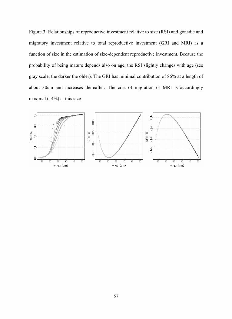
57
Figure 3: Relationships of reproductive investment relative to size (RSI) and gonadic and
migratory investment relative to total reproductive investment (GRI and MRI) as a
function of size in the estimation of size-dependent reproductive investment. Because the
probability of being mature depends also on age, the RSI slightly changes with age (see
gray scale, the darker the older). The GRI has minimal contribution of 86% at a length of
about 30cm and increases thereafter. The cost of migration or MRI is accordingly
maximal (14%) at this size.

58
Figure 4: Overall relative bias (Eq. 5) as a function of the true relative reproductive
investment q , the true relative onset of maturation , the true relative initial size 0 and
the number of years after the first spawning event maty (rounded up ( matmat tA )) in the
deterministic case of the four-trait and the three-trait estimation. The simulation was
based on all possible combinations for the observed ranges of the parameters: a {4,7}
g1/4
yr-1
, b {0.4,0.9} yr-1
, c {0.05,0.55} yr-1
and matt {1.25,5.25} yr. Contours were
obtained by fitting a non-parametric loess regression to the bias with span = 0.25 for the
two explanatory variables to be displayed. Bias becomes considerable if there are few
observations maty of the mature status, if the relative onset of maturation is very early
and if the relative reproductive investment q is small. Similar trends are found in the
three-trait estimation but with lower relative biases and q seems to have no more
influence on the bias.

59
Four-trait estimation

60
Three-trait estimation

61
Figure 5: Density distributions of the four estimated life history parameters and
relationships between parameter biases estimated on simulated data with environmental
noise. Very similar parameter distributions as from real data (see Figure 1) are obtained
in the simulation (first row), in which the covariance structure from the selected
distribution modes from real data was used. The regressions between parameter biases
(dashed lines) show that the biases of b and c are negatively correlated, whereas the bias
of )( cb is on average smaller than bias of each of its components. The strong positive
correlation between a and )( cb is a consequence of fitting to an asymptotic size: the
higher a is, the higher )( cb has to be to reach the same asymptotic size. The same
effect translates to b but not to c .

62

63
Figure 6: Relative biases in a , b , c and matt in the four-trait estimation and a , c and
matt in the three-trait estimation, resulting from environmental variation, shown as a
function of the CV in the simulated time series of a , b , and c (four-trait estimation) or
a and c (three-trait estimation). The estimated parameters are given relative to the
geometric mean of the time series of a , b , and c . The CV is given by the geometric
mean of the realized CV ’s in series of a , b and c . Black lines show a quantile
regression through these biases for the 50% (dashed line) and the 5% and 95% quantiles
(dotted lines). Notice that the biases are strictly evaluated only for matt , since the true
reference values of the varying a , b and c is not really known. Furthermore the
simulated CV ’s might be higher than those applying in nature.

64

65
Figure 7: Sensitivity of the parameters estimates a , b , c and matt to an incorrect
assumption about the allometric scaling exponent ( 4/3sim whereas 3/2fit or
5/4fit ) in the four- and the three-trait estimation. It was accounted for that different
allometric scaling exponents would result in different assumptions about the constant
maintenance by fitting the energy allocation model to the population growth curve
( 3/2b =0.175 year-1
, 4/3b =0..459 year-1
, 5/4b =0.864 year-1
, leading to different
solutions of Eq. 4). The estimated against the true parameters are shown, black dots
representing the estimates assuming the correct allometric scaling exponent ( 4/3 ),
typically on the 45º-line, light gray “-” and dark gray “+“ represent the estimates by
assuming falsely a too low ( 3/2 ) or too high ( 5/4 ) scaling exponent
respectively, whereas the light grey and dark gray dotted lines represent the regression
through these estimated and true data points assuming wrong scaling.

66

67
Figure 8: Comparison of reaction norms derived from the 3 trait estimation of individual
life history in this study (gray lines) with reaction norm estimated by from Grift, et al.
(2003) averaged over the past 5 decades by only using cohorts for which more than 30
observations were available. Dotted lines represent the 25%- and 75% probabilities of
maturation, the dashed line represents the average length at age. The reaction norm from
individual life history estimation is shown for an interpretation of the first spawning
event matA given by matt plus a minimal period of preparation for spawning of 4 months,
rounded up to the next year.