MultiPass Lvq,Logistic Model Tree,K-Star for Audio Data ...519092/FULLTEXT01.pdf · Magesh Kumar...
57
Classification of Parkinson’s Disease using MultiPass Lvq,Logistic Model Tree,K-Star for Audio Data set Magesh Kumar Udaya Kumar 2011 Master Thesis Computer Engineering Nr:E4086D
Transcript of MultiPass Lvq,Logistic Model Tree,K-Star for Audio Data ...519092/FULLTEXT01.pdf · Magesh Kumar...

Classification of Parkinson’s Disease using
MultiPass Lvq,Logistic Model Tree,K-Star
for Audio Data set
Magesh Kumar Udaya Kumar
2011
Master
Thesis
Computer
Engineering
Nr:E4086D

II
DEGREE PROJECT
Computer Engineering
Programme
Reg number Extent
Masters Programme in Computer Engineering - Applied
Artificial Intelligence
E4086D 15 ECTS
Name of student Year-Month-Day
Magesh Kumar Udaya Kumar 2011-04-02 Supervisor Examiner
Jerker Westin
Hasan Fleyeh
Company/Department Supervisor at the Company/Department
Department of Computer Engineering, Dalarna University
Jerker Westin Title
Classification of Parkinson‟s Disease using MultiPass Lvq,Logistic Model Tree,K-Star for
Audio Data set Keywords
Parkinson‟s Disease, Audio Data set, MultiPass Lvq, Logistic Model Tree, K-Star.
III
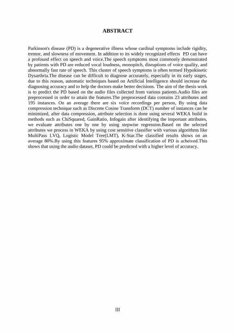
ABSTRACT
Parkinson's disease (PD) is a degenerative illness whose cardinal symptoms include rigidity,
tremor, and slowness of movement. In addition to its widely recognized effects PD can have
a profound effect on speech and voice.The speech symptoms most commonly demonstrated
by patients with PD are reduced vocal loudness, monopitch, disruptions of voice quality, and
abnormally fast rate of speech. This cluster of speech symptoms is often termed Hypokinetic
Dysarthria.The disease can be difficult to diagnose accurately, especially in its early stages,
due to this reason, automatic techniques based on Artificial Intelligence should increase the
diagnosing accuracy and to help the doctors make better decisions. The aim of the thesis work
is to predict the PD based on the audio files collected from various patients.Audio files are
preprocessed in order to attain the features.The preprocessed data contains 23 attributes and
195 instances. On an average there are six voice recordings per person, By using data
compression technique such as Discrete Cosine Transform (DCT) number of instances can be
minimized, after data compression, attribute selection is done using several WEKA build in
methods such as ChiSquared, GainRatio, Infogain after identifying the important attributes,
we evaluate attributes one by one by using stepwise regression.Based on the selected
attributes we process in WEKA by using cost sensitive classifier with various algorithms like
MultiPass LVQ, Logistic Model Tree(LMT), K-Star.The classified results shows on an
average 80%.By using this features 95% approximate classification of PD is acheived.This
shows that using the audio dataset, PD could be predicted with a higher level of accuracy.

IV
ACKNOWLEDGEMENT
I want to express my gratitude to all the people who have given their heart whelming
full support in making this compilation a magnificent experience.
First and foremost I offer my sincerest gratitude to my supervisor, Mr. Jerker Westin,
who has supported me throughout my thesis with his patience and knowledge.
I also thank Mr. Hasan Fleyeh, Mr. Siril Yella and Mr. Taha Khan for their support
and initiative to induce knowledge to their subordinates.
I can‟t forget to thank my family and friends who have inspired, encouraged and fully
supported me for every endeavour of mine and backed me to surpass the hurdles that come
my way.
V
TABLE OF CONTENTS
1. INTRODUCTION
1.1 Problem Description: ......................................................................................................... 2
1.2 Objective: ............................................................................................................................ 3
1.3 Why Audio Data: ................................................................................................................ 3
2. THEORETICAL BACKGROUND
2.1 Cross validation: ................................................................................................................. 4
2.2 Dataset Information: .......................................................................................................... 4
2.3 Cost Matrix: ........................................................................................................................ 5
2.4 Evaluating Methods: .......................................................................................................... 5
2.4.1 Chi-squared Attribute Evaluation: ................................................................................ 5
2.4.2 Gain Ratio Attribute Evaluation: .................................................................................. 5
2.4.3 Info Gain Attribute Evaluation: .................................................................................... 6
2.4.4 Stepwise Regression: ....................................................................................................... 6
2.5 Classification Methods: ...................................................................................................... 6
2.5.1 Cost Sensitive Function: ................................................................................................. 6
2.5.2 Multipass LVQ: ............................................................................................................... 7
2.5.3 Logistic Model Tree: ....................................................................................................... 8
2.5.4 K* Algorithm: ................................................................................................................ 10
3. METHODOLOGY
3.1 Attribute Calculation: ...................................................................................................... 11
3.2 Acoustics Analysis ............................................................................................................ 11
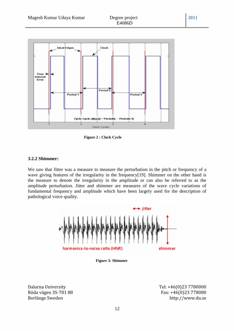
3.2.1 Jitter: .............................................................................................................................. 11
3.2.2 Shimmer: ........................................................................................................................ 12
3.3 Features: ............................................................................................................................ 13
3.3.1 Jitter (Local) .................................................................................................................. 13
3.3.2 Jitter (Local, Absolute): ................................................................................................ 13
3.3.3 Jitter (RAP): .................................................................................................................. 14
3.3.4 Jitter (PPQ5): ................................................................................................................. 14
3.3.5 Jitter (DDP): .................................................................................................................. 15
VI
3.3.6 Shimmer (Local): ........................................................................................................... 15
3.3.7 Shimmer (Local , Db): .................................................................................................. 16
3.3.8 Shimmer (APQ3): .......................................................................................................... 16
3.3.9 Shimmer (APQ5): .......................................................................................................... 16
3.3.10 Shimmer (APQ11): ...................................................................................................... 16
3.3.11 Shimmer (DDP): .......................................................................................................... 17
3.3.12 Detrended Fluctuation Analysis (DFA): ................................................................... 17
3.3.13 Harmonic to Noise Ratio (HNR): ............................................................................... 18
3.3.14 Recurrence Period Density Entropy (RPDE): .......................................................... 19
3.3.15 Pitch Period Entropy (PPE): ...................................................................................... 19
3.3.16 Noise to Harmonic Ratio (NHR): ............................................................................... 20
3.3.17 Average fundamental frequency (Fo): ...................................................................... 20
3.3.18 Lowest fundamental frequency (Flo): ....................................................................... 20
3.3.19 Highest fundamental frequency (Fhi): ...................................................................... 21
3.3.20 Correlation Dimension (D2): ...................................................................................... 21
3.3.21 Spread1: ....................................................................................................................... 21
3.3.22 Spread2: ....................................................................................................................... 22
3.4 Related Work: .................................................................................................................. 22
3.5 Proposed System: ............................................................................................................. 24
3.6 Data Pre-processing: ........................................................................................................ 24
3.7 Feature Extraction: .......................................................................................................... 24
3.7.1 DCT: ............................................................................................................................... 25
3.8 Visualizing all the attributes ............................................................................................ 26
3.9 Attribute Selection ............................................................................................................ 27
3.9.1 Chi squared Attribute Evaluation ............................................................................... 27
3.9.2 Gain Ratio Attribute Evaluation: ................................................................................ 28
3.9.3 Info Gain Attribute Evaluation: .................................................................................. 29
3.9.4 Stepwise Regression: ..................................................................................................... 30
VII
4. RESULT AND ANALYSIS:
4.1 Multipass LVQ: ................................................................................................................ 38
4.2 Logistic Model Tree ......................................................................................................... 39
4.3 K-Star Algorithm ............................................................................................................. 40
4.4 Results of Selected Attributes: ........................................................................................ 41
4.5 Results of Various Classifiers: ........................................................................................ 42
4.5.1 Comparison .................................................................................................................... 43
4.5.2 Multipass LVQ: ............................................................................................................. 43
4.5.3 Logistic Model Tree: ..................................................................................................... 44
4.5.4 K-Star Algorithm: ......................................................................................................... 44
CONCLUSION AND FUTURE WORK .............................................................................. 45
REFERENCES ....................................................................................................................... 47

VIII
LIST OF FIGURES
Figure 1: Jitter ........................................................................................................................ 11 Figure 2 : Clock Cycle ............................................................................................................ 12 Figure 3: Shimmer ................................................................................................................. 12
Figure 4: Detrended Fluctuation Analaysis ......................................................................... 18 Figure 5: Harmonic to Noise Ratio ....................................................................................... 19 Figure 6: Discrete Fourier Transform.................................................................................. 25 Figure 7: Visualizing all the Attributes ................................................................................ 26 Figure 8: MultiPass LVQ ...................................................................................................... 38
Figure 9: Logistic Model Tree ............................................................................................... 39
Figure 10: K-Star Algorithm ................................................................................................. 40

IX
LIST OF TABLES
Table 1: Chi squared .............................................................................................................. 27
Table 1: Gain Ratio ……........................................................................................................28
Table 2: Info Gain .................................................................................................................. 29
Table 3(i): Stepwise Regression ............................................................................................ 31
Table 4(ii) : Adding two attribute in stepwise regression ................................................... 32
Table 4(iii) : Fhi values in all the steps ................................................................................. 32
Table 4(iv) : Spread 1 value in all the steps ......................................................................... 33
Table 4(v): Final combination of features using stepwise regression ................................ 33
Table 5: Time Evaluation ..................................................................................................... 34
Table 6: Features Description of the Audio Dataset ........................................................... 35
Table 7 (i): Results of Selected Attributes ............................................................................ 41
Table 7 (ii): Results of Selected Attributes ........................................................................... 41
Table 8 (i) : Results of Various Classifiers ........................................................................... 42
Table 8 (ii) : Results of Various Classifiers .......................................................................... 42
Table 9 : Comparison ............................................................................................................. 43
Table 10 : Confusion Matrix of Multipass LVQ ................................................................. 43
Table 11 : Confusion Matrix of Logistic Model tree ........................................................... 44
Table 12 : Confusion Matrix of K-Star Algorithm ............................................................. 44
Magesh Kumar Udaya Kumar Degree project
E4086D 2011
Dalarna University Tel: +46(0)23 7780000 Röda vägen 3S-781 88 Fax: +46(0)23 778080 Borlänge Sweden http://www.du.se
1
INTRODUCTION
Parkinson's disease (PD) is a degenerative disorder of the central nervous system [1]. It results
from the death of dopamine-containing cells in the substantia nigra, a region of the midbrain ,
that often impairs the sufferer's motor skills, speech, and other functions. As these symptoms
become more pronounced, patients may have difficulty walking, talking, or completing other
simple tasks.The disease can be difficult to diagnose accurately, especially in its early stages.
PD is more common in the elderly with most cases occurring after the age of 50. PD is both
chronic, it persists over a long period of time, and progressive. A
motor speech disorder caused by damage to the part of the brain called the basal ganglia
which in turn affects the muscles involved in speech[2].The causes for Hypokinetic Dysarthia
include infection, tumour and ataxic cerebral palsy. The most affected by the Parkinson
disease are those of the age above 50. There are also few cases of the Parkinson‟s disease to
affect at younger ages and it affects both the genders. Like several other diseases the
Parkinson‟s disease is also hereditary. The conditions where people of younger age are
affected are mostly because of the family history of the diseases. Parkinson's in children may
occur because the nerves are not as sensitive to dopamine. Parkinson's is rare in children[2].
In order to control the body muscle movement the nerve cells use a brain chemical called
dopamine. Parkinson's disease is the condition when these nerve cells that produce the
dopamine are slowly destroyed. In the absence of dopamine the nerve cells in that part of the
brain cannot properly communicate with the other parts. This tends to loss of functionalities.
Though the proper reason for the depletion of these brain cells is still unknown, we know that
it gets worse by time. Untreated, the disorder will get worse until a person is totally disabled.
Parkinson's may lead to a deterioration of all brain functions, and an early death.In addition to
its widely recognized effects on gait, posture, balance, and upper limb coordination, PD can
have a profound effect on speech and voice. Although symptoms vary widely from patient to
patient, the speech symptoms most commonly demonstrated by patients with PD are reduced
vocal loudness, monopitch, disruptions of voice quality, and abnormally fast rate of
speech[2]. This cluster of speech symptoms is often termed Hypokinetic Dysarthria. The most
common symptom of Hypokinetic Dysarthria is Hypophonia, or reduced vocal loudness.
Patients demonstrating this symptom may be unaware of the volume at which they are
speaking and may require frequent requests to speak louder.
The symptoms can be very evident and is usually mild at the beginning and then get more
complex and the functionality lost varies on several conditions. The list of signs and
symptoms mentioned in various sources for Hypokinetic Dysarthria includes the 7 symptoms
listed below[2]:
Hoarse voice
Breath voice
Coarse voice
Tremulous voice
Single pitched voice
Monotone voice
Sudden pitch changes
Magesh Kumar Udaya Kumar Degree project
E4086D 2011
Dalarna University Tel: +46(0)23 7780000 Röda vägen 3S-781 88 Fax: +46(0)23 778080 Borlänge Sweden http://www.du.se
2
Though the health care providers could diagnose the presence of Parkinson‟s disease based on
the symptoms by the physical examination, the assess ability of the symptoms becomes
difficult more particularly in case of elderly people[2]. As the illness progresses the signs like
tremor, walking problem and speech variations becomes clearer. The main point that the
diagnosis must concentrate on ruling out the other ailments that share the similar symoptoms.
The signs that need to be looked for are:
Slow opening and inadequate closing of the vocal folds
Slows down voluntary movements
1.1 Problem Description:
There are many research works going on Parkinson disease(PD) which seemed to be the
second most common disease in the world and it still more increasing nowever day‟s .This
situation leads to build a decision support system for PD. Now ever day‟s computational tools
have been designed for helping the doctors to make decision about their patients.
Artificial Intelligence techniques are one of the most powerful and widely used techniques
now ever days by experts. Classification system can improve the accuracy and reliability of
diagnoses and minimizing the errors.
For many Parkinson disease people, the necessary of physical visits to the clinic for
monitoring and treatment are difficult. Widening access to the Internet and advanced
telecommunication systems bandwidth offers the possibility of remote monitoring of patients,
with substantial opportunities for lowering the inconvenience and cost of physical visits.
However, in order to exploit these opportunities, there is the need for reliable clinical
monitoring tools.
Speech pathologists have been trying to get their patients with Parkinson‟s disease to raise
their voices for years. Although the condition is primarily characterized by tremors and
difficulty in walking, most patients also suffer from speech problems, particularly slurring and
what‟s known in the field as weak voice. While 89% of people with PD experience some type
of speech problems.So if the clasification percentage of Parkinson disease is high then its
possible to predict parkinson in early stages.
Typically, the diagnosis is based on medical summary and neurological examination
conducted by interviewing and observing the patient in person using the Unified Parkinson's
Disease Rating Scale (UPDRS). It is very difficult to predict PD based on UDPRS in early
stages, only 75% of clinical diagnoses of PD are confirmed to be idiopathic PD at autopsy.
Thus, automatic techniques based on Artificial Intelligence are needed to increase the
diagnosis accuracy and to help Doctors to make better decisions.
Magesh Kumar Udaya Kumar Degree project
E4086D 2011
Dalarna University Tel: +46(0)23 7780000 Röda vägen 3S-781 88 Fax: +46(0)23 778080 Borlänge Sweden http://www.du.se
3
1.2 Objective:
The main objective of this paper is to identify Parkinson disease (PD) based on the speech
features. One who is having PD has some disturbance in voice based on that disturbances we
can be able to identify PD.The idea behind this thesis work is to predict the PD based on the
audio data. Based on the several methods of calculating feautures of audio format several
features are obtained.The data contains several attributes, our goal is to reduce the no of
attributes and attain a good classification percentage. And try to minimize False Positives as
much as possible.
1.3 Why Audio Data:
Research has shown that approximately 90% of PWP (people with Parkinson‟s disease)
exhibit some form of vocal impairment [3].Voice measurement to detect and track the
symptoms of PD has drawn significant attention.PWP display a some sought of vocal
symptoms that include,
Impairment in the normal production of vocal sounds (dysphonia)
Problems with the normal articulation of speech (dysarthria)
Dysphonic symptoms typically include reduced loudness, breathiness, roughness, decreased
energy in the higher parts of the harmonic spectrum, and exaggerated vocal tremor.
Voice disorders may be due to a physical problem, such as vocal nodules or polyps, which are
almost like a callous on the vocal cord, paralysis of the vocal cords because of strokes or after
some surgeries, or contact ulcers on the vocal cords [4]. These disorders may also be caused
by misuse of the vocal instrument, such as using the voice too high or low in pitch, using the
voice too softly or too loudly, or with insufficient breath support, often because of postural
problems.
Magesh Kumar Udaya Kumar Degree project
E4086D 2011
Dalarna University Tel: +46(0)23 7780000 Röda vägen 3S-781 88 Fax: +46(0)23 778080 Borlänge Sweden http://www.du.se
4
Chapter 2
THEORETICAL BACKGROUND
2.1 Cross validation:
Classifiers rely on being trained before they can reliably be used on new data. Of course, it
stands to reason that the more instances the classifier is exposed to during the training phase,
the more reliable it will be as it has more experience. However, once trained, we would like to
test the classifier too, so that we are confident that it works successfully. For this, yet more
unseen instances are required[14].
A problem which often occurs is the lack of readily available training/test data. These
instances must be pre-classified which is typically time-consuming (hence the reason we are
trying to automate it with a software classifier ) a nice method to circumvent this issue is
know as cross-validation[14]. It works as follows:
1. Separate data in to fixed number of partitions (or folds)
2. Select the first fold for testing, whilst the remaining folds are used for training.
3. Perform classification and obtain performance metrics.
4. Select the next partition as testing and use the rest as training data.
5. Repeat classification until each partition has been used as the test set.
6. Calculate an average performance from the individual experiments.
This allows the use of the maximum amount of data to create the model at the same time
getting a good estimate for the expected error rate. The error estimate obtained using the cross
validation is usually a better estimate of the true error rate than that obtained by just having 1
validation dataset as the whole dataset will be used to estimate the true error rate.
2.2 Dataset Information:
This Parkinson database used in this study is taken from the University of California at Irvine.
This dataset is composed of a range of biomedical voice measurements from 32 peoples out of
which 24 are affected by Parkinson disease. The ages of the subjects ranged from 46 to 85
years (mean = 65.8). Each column represents a particular voice measure and each row
corresponds one of 195 voice recording from these individuals. On an average there are six
recordings per patient. Each recording is ranged from one to 36 seconds in length. The main
aim of the data is to discriminate healthy people from those of PD. This Phonation‟s were
recorded in an IAC sound-treated booth using a head-mounted microphone. The voice signals
were recorded directly to the computer using Kay Elemetrics, sampled at 44.1 kHz, with 16
bit resolution.
Magesh Kumar Udaya Kumar Degree project
E4086D 2011
Dalarna University Tel: +46(0)23 7780000 Röda vägen 3S-781 88 Fax: +46(0)23 778080 Borlänge Sweden http://www.du.se
5
2.3 Cost Matrix:
To explain cost matrix let us assume a case where all misclassifications had equal weights and
target values that appear less frequently would not be privileged. You might obtain a model
that misclassifies these less frequent target values while achieving a very low overall error
rate. To improve classification decision trees and to get better models with such 'skewed data',
the tree heuristic automatically generates an appropriate cost matrix to balance the distribution
of class labels when a decision tree is trained. You can also manually adjust the cost matrix.
..............................................(1)
2.4 Evaluating Methods:
2.4.1 Chi-squared Attribute Evaluation:
The feature Selection using chi square test is a very commonly used method. This particular
method evaluates features individually by measuring their Chi Squared statistic with respect
to the classes. It is a widely used standard feature selection method.
The range of each feature is subdivided in a number of intervals, and then for each interval the
number of expected instances for each class is compared with the actual number of instances.
This difference is squared, and the sum of these differences for all intervals, divided by the
total number of instances, is the X^2 value of that feature.
2.4.2 Gain Ratio Attribute Evaluation:
The Gain Ratio evaluates the worth of an attribute by measuring the gain ratio with respect to
the class. The gain ratio takes into account the number and size of the generated child nodes
from a candidate split. This is done by a measure that is called intrinsic information. If a given
split will branch a node into X child nodes, the intrinsic information is calculated as follows:
Intrinsic_Info (t) = - ..............................................(2)
Nx is the number of instances in child node X.
For a given split s on the node t, the gain ratio is then defined as the follows:
Gain_Ratio (t) = ..............................................(3)
The gain ratio measure will thus penalize highly branching attributes and will avoid the bias
associated with just using the information gain measure.
Magesh Kumar Udaya Kumar Degree project
E4086D 2011
Dalarna University Tel: +46(0)23 7780000 Röda vägen 3S-781 88 Fax: +46(0)23 778080 Borlänge Sweden http://www.du.se
6
In many cases though, just using the gain ratio measure alone can lead to problems as it can
overcompensate for the bias. A given split can be selected just because it has a small value for
the intrinsic information. A common workaround is to consider first, only splits that have
above average information gain and then compare their gain ratios.
2.4.3 Info Gain Attribute Evaluation:
This evaluates the worth of an attribute by measuring the information gain with respect to the
class. InfoGain(Class,Attribute) = H(Class) - H(Class | Attribute) / H(Attribute) ..............................................(4)
2.4.4 Stepwise Regression:
Stepwise regression removes and adds variables to the regression model for the purpose of
identifying a useful subset of the predictors. Minitab provides three commonly used
procedures: standard stepwise regression (adds and removes variables), forward selection
(adds variables), and backward elimination (removes variables).
In this thesis, we use standard stepwise regression to evaluate our data. We evaluate attributes
one by one with mainly comparing their P-Values to estimate their significance individually.
P-value: P-value for each coefficient tests the null hypothesis that the coefficient is equal to
zero (no effect). Therefore, low p-values suggest the predictor is a meaningful addition to
your model. The next values are used to select model which is the best fit:
S: S is measured in the units of the response variable and represents the standard distance
data values fall from the regression line, or the standard deviation of the residuals. For a given
study, the better the equation predicts the response, the lower the value of S.
R-sq: The proportion of the variation in the response data explained by the model. For the
value of R-sq , the larger the better .
2.5 Classification Methods:
2.5.1 Cost Sensitive Function:
Cost-sensitive classification is one of mainstream research topics in data mining and machine
learning that induces models from data with unbalance class distributions and impacts by
quantifying and tackling the unbalance. Rooted in diagnosis data analysis applications, there
are great many techniques developed for cost-sensitive learning[15]. They are mainly focused
on minimizing the total cost of misclassification costs, test costs, or other types of cost, or a
combination among these costs.
Weka treats all types of classification errors equally. In many practical cases though, not all
errors are equal. If the costs are known, it is possible to use this information to build a cost
sensitive model or to alter model predictions to minimize expected costs. The way to do this
Magesh Kumar Udaya Kumar Degree project
E4086D 2011
Dalarna University Tel: +46(0)23 7780000 Röda vägen 3S-781 88 Fax: +46(0)23 778080 Borlänge Sweden http://www.du.se
7
in Weka is to create cost files[15]. Cost files are small text files that define a cost matrix. An
example of this is shown below:
% Rows Columns
2 2
% Matrix elements
0 2
1 0
2.5.2 Multipass LVQ:
Linear Vector Quantization (LVQ)
A competitive learning algorithm said to be a supervised version of the Self-Organizing Map
(SOM) algorithm by Kohonen Goal of the algorithm is to approximate the distribution of a
class using a reduced number of codebook vectors where the algorithm seeks to minimise
classification errors Codebook vectors become exemplars for a particular class, attempting to
represent class boundaries [16]. The algorithm does not construct a topographical ordering of
the dataset (there is no concept of explicit neighbourhood in LVQ as there is in the SOM
algorithm) Algorithm was proposed by Kohonen in 1986 as an improvement over Labelled
Vector Quantization the algorithm is associated with the neural network class of learning
algorithms, though works significantly differently compared to conventional feed-forward
networks like Back Propagation [16].
LVQ1 - A single BMU (best matching unit) is selected and moved closer or further
away from each data vector, per iteration.
OLVQ1 (Optimised LVQ1) - The same as LVQ1, except that each codebook vector
has its own learning rate.
LVQ2.1 - Two BMU's are selected and only updated if one belongs to the desired
class and one does not, and the distance ratio is within a defined window.
LVQ3 - The same as LVQ2.1 except if both BMU's are of the correct class, they are
updated but adjusted using an epsilon value (adjusted learning rate instead of the
global learning rate).
Pass 1
OLVQ1 recommended for fast approximation
Intended to quickly and roughly approximate the class distribution
Larger learning rates and shorter training times should be used
Learning rate (0.1 to 0.4 - say 0.3)
Training iterations (30 to 50 times the number of codebook vectors)
Magesh Kumar Udaya Kumar Degree project
E4086D 2011
Dalarna University Tel: +46(0)23 7780000 Röda vägen 3S-781 88 Fax: +46(0)23 778080 Borlänge Sweden http://www.du.se
8
Pass 2
LVQ1 or LVQ3 recommended for fine tuning
Intended to slowly and precisely finetune the codebook vectors to the class
distribution in the data
Smaller learning rates and longer training times should be used
Learning rate (< 0.1 - say 0.05)
Training iterations (about 10 times that of the first pass)
Thought we have all the theories and implementation procedures proven to be yielding
positive results the accuracy of classification and the generalization and the learning speed
depend on several factors.
The LVQ algorithm is trained much faster when compared to the other available ANN
techniques like the Back Propagation. The LVQs makes it possible to reduce large datasets to
a smaller number of codebook vectors suitable for classification or visualization.It provides a
level of robustness its ability to generalize features in the provided dataset.If we are able to
compare the attributes using a meaningful distance measure then we can approximate just
about any classification problem.Like in the nearest neighbor techniques we have unlimited
number of dimensions in the codebook vectors.We do not have to Normalize the input
date.We can use input data with some missing values and the LVQ will still handle There are
aslo some disadvantages namely,it has to generate distance measures for all the attributes and
the accuracy of the model is highly dependent on several factors such as the initialization of
the model, the learning parameters like the learning rate,training iteration,ect., and the class
distribution in the training dataset.
2.5.3 Logistic Model Tree:
A logistic model tree or LMT basically consists of a standard decision tree structure with
logistic regression functions at the leaves very much like a model tree which is a regression
tree with regression functions at the leaves[17]. As in ordinary decision trees, a test on one of
the attributes is associated with every inner node. For a nominal (enumerated) attribute with k
values, the node has k child nodes, and instances are sorted down one of the k branches
depending on their value of the attribute. For numeric attributes, the node has two child nodes
and the test consists of comparing the attribute value to a threshold an instance is sorted down
the left branch if its value for that attribute is smaller than the threshold and sorted down the
right branch otherwise.
Classifier for building 'logistic model trees' which are classification trees with logistic
regression functions at the leaves[17]. The algorithm can deal with binary and multi-class
target variables, numeric and nominal attributes and missing values
We can take a look at the types of parameters the LMT deals with:
Magesh Kumar Udaya Kumar Degree project
E4086D 2011
Dalarna University Tel: +46(0)23 7780000 Röda vägen 3S-781 88 Fax: +46(0)23 778080 Borlänge Sweden http://www.du.se
9
B: Binary splits (convert nominal attributes to binary ones)
R: Split on residuals instead of class values
C: Use cross-validation for boosting at all nodes (i.e., disable heuristic)
P: Use error on probabilities instead of misclassification error for stopping criterion
of LogitBoost.
I : Set fixed number of iterations for LogitBoost instead of using cross-validation
M: Set minimum number of instances at which a node can be split with a default 15
W: Set beta for weight trimming for LogitBoost. Set to 0 (default) for no weight
trimming.
A: The AIC is used to choose the best iteration.
Building Logical Model Trees:
An algorithm for building logistic model trees has to address the following issues:
1. Growing the tree
There is a straightforward approach for growing logistic model trees that follows the way
trees are built by M5. This involves first building a standard classification tree using the C4.5
algorithm then building a logistic regression model at every node trained on the set of
examples at that node[17]. In this approach, the logistic regression models are built in
isolation on the local training examples at a node.
2. Building the logistic models
We chose a different approach for constructing the logistic regression functions, namely by
incrementally refining logistic models already fit at higher levels in the tree. Assume we have
split a node and want to build the logistic regression function at one of the child nodes[17].
Since we have already fit a logistic regression at the parent node, it is reasonable to use it as a
basis for fitting the logistic regression at the child. We expect that the parameters of the model
at the parent node already encode „global‟ influences of some attributes on the class variable,
at the child node, the model can be further refined by taking into account influences of
attributes that are only valid locally, i.e. within the set of training examples associated with
the child node.
3. Pruning
Pruning is an important issue for logistic model trees. The pruning scheme has to decide
whether a linear logistic regression model (a tree pruned back to the root) or a more elaborate
tree structure is preferable for a particular dataset. It has been shown that this depends on the
size and characteristics of the dataset.
Magesh Kumar Udaya Kumar Degree project
E4086D 2011
Dalarna University Tel: +46(0)23 7780000 Röda vägen 3S-781 88 Fax: +46(0)23 778080 Borlänge Sweden http://www.du.se
10
2.5.4 K* Algorithm:
The K* algorithm in terms of statistics and data mining can be defined as a method of cluster
analysis which mainly aims at the partition of „n‟ observation into „k‟ clusters in which each
observation belongs to the cluster with the nearest mean[18]. We can describe K* algorithm
as an instance based learner which uses entropy as a distance measure. The benifits are that it
provides a consistent approach to handling of symbolic attributes, real valued attributes and
missing values.
Instance-based learners classify an instance by comparing it to a database of pre-classified
examples. Nearest neighbor algorithms are the simplest of instance-based learners. They use
some domain specific distance function to retrieve the single most similar instance from the
training set. The k nearest neighbors of the new instance is retrieved and whichever class is
predominant amongst them is given as the new instance's classification.
Entropy as a distance measure:
The approach that is taken here is to compute the distance between two instances by the
concept of information theory where the distance between instances can be defined as the
complexity of transforming one instance into another. The calculation of the complexity is
done by taking a finite set of transformations which map instances to instances is defined
The probability function P* is defined as the probability of all paths from instance „a‟ to
instance „b‟:
P*(b|a) = ..............................................(5)
The K* function is then defined as:
K*(b | a) = - p*(b | a) ..............................................(6)
K* is not strictly a distance function. For example, K * (a|a) is in general non-zero
and the function (as emphasized by the | notation) is not symmetric.
Magesh Kumar Udaya Kumar Degree project
E4086D 2011
Dalarna University Tel: +46(0)23 7780000 Röda vägen 3S-781 88 Fax: +46(0)23 778080 Borlänge Sweden http://www.du.se
11
Chapter 3
METHODOLOGY
3.1 Attribute Calculation:
Before we go any further in discussing about the features of noise waves we first need to
understand certain properties of waves. Every set of waves have individual characteristics.
This is the main requirement in order to differentiate between two types of waves by which
we also understand that all waves are not equal and differ with several attributes. Each wave
has its own specific face which we need to identify and for that we go on to consider the three
important characteristics of waves: Frequency, Wavelength and Amplitude. Now let us go
ahead and take a closer look to understand what these characteristics actually are and how
they define the peculiarity of the wave.
3.2 Acoustics Analysis:
Perceptual assessment of voice is analysis of the voice solely by listening. Formal perceptual
evaluation typically uses a published protocol to systematically describe characteristics of
voice disorder. Acoustic analysis is more or less the objective counterpart of perceptual
assessment of voice where it measures several of the same vocal characteristics that are
explored using auditory perception like pitch, pitch range, loudness, degree of hoarseness.
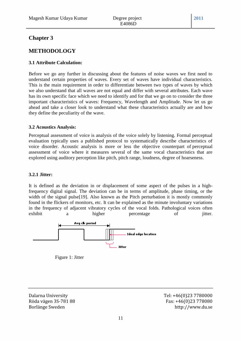
3.2.1 Jitter:
It is defined as the deviation in or displacement of some aspect of the pulses in a high-
frequency digital signal. The deviation can be in terms of amplitude, phase timing, or the
width of the signal pulse[19]. Also known as the Pitch perturbation it is mostly commonly
found in the flickers of monitors, etc. It can be explained as the minute involuntary variations
in the frequency of adjacent vibratory cycles of the vocal folds. Pathological voices often
exhibit a higher percentage of jitter.
Figure 1: Jitter
Magesh Kumar Udaya Kumar Degree project
E4086D 2011
Dalarna University Tel: +46(0)23 7780000 Röda vägen 3S-781 88 Fax: +46(0)23 778080 Borlänge Sweden http://www.du.se
12
Figure 2 : Clock Cycle
3.2.2 Shimmer:
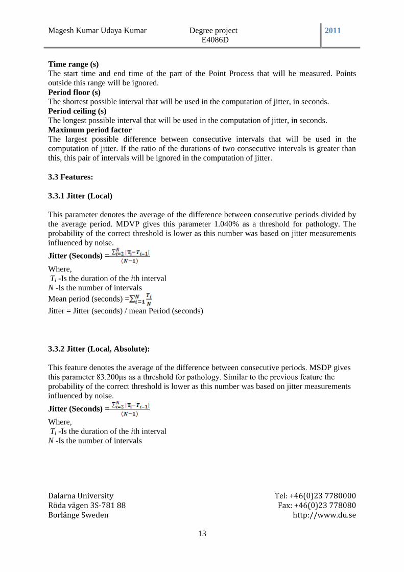
We saw that Jitter was a measure to measure the perturbation in the pitch or frequency of a
wave giving features of the irregularity in the frequency[19]. Shimmer on the other hand is
the measure to denote the irregularity in the amplitude or can also be referred to as the
amplitude perturbation. Jitter and shimmer are measures of the wave cycle variations of
fundamental frequency and amplitude which have been largely used for the description of
pathological voice quality.
Figure 3: Shimmer
Magesh Kumar Udaya Kumar Degree project
E4086D 2011
Dalarna University Tel: +46(0)23 7780000 Röda vägen 3S-781 88 Fax: +46(0)23 778080 Borlänge Sweden http://www.du.se
13
Time range (s)
The start time and end time of the part of the Point Process that will be measured. Points
outside this range will be ignored.
Period floor (s)
The shortest possible interval that will be used in the computation of jitter, in seconds.
Period ceiling (s)
The longest possible interval that will be used in the computation of jitter, in seconds.
Maximum period factor
The largest possible difference between consecutive intervals that will be used in the
computation of jitter. If the ratio of the durations of two consecutive intervals is greater than
this, this pair of intervals will be ignored in the computation of jitter.
3.3 Features:
3.3.1 Jitter (Local)
This parameter denotes the average of the difference between consecutive periods divided by
the average period. MDVP gives this parameter 1.040% as a threshold for pathology. The
probability of the correct threshold is lower as this number was based on jitter measurements
influenced by noise.
Jitter (Seconds) =
Where,
Ti -Is the duration of the ith interval
N -Is the number of intervals
Mean period (seconds) =
Jitter = Jitter (seconds) / mean Period (seconds)
3.3.2 Jitter (Local, Absolute):
This feature denotes the average of the difference between consecutive periods. MSDP gives
this parameter 83.200μs as a threshold for pathology. Similar to the previous feature the
probability of the correct threshold is lower as this number was based on jitter measurements
influenced by noise.
Jitter (Seconds) =
Where,
Ti -Is the duration of the ith interval
N -Is the number of intervals
Magesh Kumar Udaya Kumar Degree project
E4086D 2011
Dalarna University Tel: +46(0)23 7780000 Röda vägen 3S-781 88 Fax: +46(0)23 778080 Borlänge Sweden http://www.du.se
14
3.3.3 Jitter (RAP):
This is the Relative Average Perturbation, the average absolute difference between a period
and the average of it and its two neighbors, divided by the average period. MSDP gives this
parameter 0.680% μs as a threshold for pathology. Similar to the previous two features the
probability of the correct threshold is lower as this number was based on jitter measurements
influenced by noise.Relative Average Perturbation is defined in terms of three consecutive
intervals, as follows,
First, we define the absolute (i.e. non-relative) Average Perturbation (in seconds):
absAP (seconds) =
Second, we define the mean period as,
meanPeriod(seconds) =
Finally, we compute the Relative Average Perturbation as,
RAP = absAP(seconds) / meanPeriod(seconds)
3.3.4 Jitter (PPQ5):
It is similar to the JITTER(RAP) feature but with 5 points. In this parameter we see the five-
point Period Perturbation Quotient, the average absolute difference between a period and the
average of it and its four closest neighbours, divided by the average period. MSDP gives this
parameter 0.840% μs as a threshold for pathology. Similar to the other features the probability
of the correct threshold is lower as this number was based on jitter measurements influenced
by noise.
The five-point Period Perturbation Quotient (PPQ5) is defined in terms of five consecutive
intervals, as follows,
First, we define the absolute (i.e. non-relative) PPQ5 (in seconds):
absPPQ5 (Seconds) =
Second, we define the mean period as
Mean period (seconds) =
Finally, we compute the five-point Period Perturbation Quotient as

Magesh Kumar Udaya Kumar Degree project
E4086D 2011
Dalarna University Tel: +46(0)23 7780000 Röda vägen 3S-781 88 Fax: +46(0)23 778080 Borlänge Sweden http://www.du.se
15
3.3.5 Jitter (DDP):
We can see in this feature that average absolute difference between consecutive differences
between consecutive periods, divided by the average period. The value equals three times
RAP.
First, we define the absolute (i.e. non-relative) Average Perturbation (in seconds) as one third
of the mean absolute (non-negative) difference of difference of consecutive intervals:
AbsDDP (seconds) =
Second, we define the mean period as
Mean period (seconds) =
Finally, we compute DDP as
3.3.6 Shimmer (Local):
In this feature we can see the difference between the amplitudes of consecutive periods,
divided by the average amplitude. MSDP gives this parameter 3.810% as a threshold for
pathology.
Average absolute difference =

Magesh Kumar Udaya Kumar Degree project
E4086D 2011
Dalarna University Tel: +46(0)23 7780000 Röda vägen 3S-781 88 Fax: +46(0)23 778080 Borlänge Sweden http://www.du.se
16
3.3.7 Shimmer (Local , Db):
It is the average absolute base-10 logarithm of the difference between the amplitudes of
consecutive periods, multiplied by 20. MSDP gives this parameter 0.350 dB as a threshold for
pathology.
3.3.8 Shimmer (APQ3):
Here we see a three point Amplitude Perturbation Quotient which is the average absolute
difference between the amplitude of a period and the average of the amplitudes of its
neighbours, divided by the average amplitude.
APQ3 =
3.3.9 Shimmer (APQ5):
Similar to the previous feature here again we see a five-point Amplitude Perturbation
Quotient which is the average absolute difference between the amplitude of a period and the
average of the amplitudes of it and its four closest neighbours, divided by the average
amplitude.
APQ5 =
3.3.10 Shimmer (APQ11):
This is the 11-point Amplitude Perturbation Quotient, the average absolute difference
between the amplitude of a period and the average of the amplitudes of it and its ten closest
neighbours, divided by the average amplitude. MSDP gives this parameter 3.810% as a
threshold for pathology.
APQ11 =
Magesh Kumar Udaya Kumar Degree project
E4086D 2011
Dalarna University Tel: +46(0)23 7780000 Röda vägen 3S-781 88 Fax: +46(0)23 778080 Borlänge Sweden http://www.du.se
17
3.3.11 Shimmer (DDP):
This is the average absolute difference between consecutive differences between the
amplitudes of consecutive periods. This is Praat's original Get shimmer. The value is three
times APQ3.
First, we define the absolute (i.e. non-relative) Average Perturbation (in seconds) as one third
of the mean absolute (non-negative) difference of difference of consecutive intervals:
AbsDDP (seconds) =
Second, we define the mean period as
Mean period (seconds) =
Finally, we compute DDP as
DDP=
3.3.12 Detrended Fluctuation Analysis (DFA):
We must understand the concept that a bounded time series can be mapped to a self-similar
process. However, another challenge investigators face while applying this type of fractal
analysis to physiologic data is that these time series are often highly non-stationary. A
simplified and general definition characterizes a time series as stationary if the mean, standard
deviation and higher moments, as well as the correlation functions are invariant under time
translation. Signals that do not obey these conditions are non-stationary. The integration
procedure will further exaggerate the non-stationary of the original data.
It is a method for determining the statistical self-affinity of a signal. It is useful for analyzing
time series that appear to be long memory process.It is similar to autocorrelation and Fourier
Transform[20].
y (k) =
Bi- The ith
interbeat Interval
Bave- The average interbeat Interval
2

Magesh Kumar Udaya Kumar Degree project
E4086D 2011
Dalarna University Tel: +46(0)23 7780000 Röda vägen 3S-781 88 Fax: +46(0)23 778080 Borlänge Sweden http://www.du.se
18
To overcome this complication we can use the modified root mean square analysis of a
random walk termed detrended fluctuation analysis for the analysis of biological data.
The integrated time series into boxes of equal length n, in each box of length n. A least
squares line is fit to the data (Representing trend in that box).
Figure 4: Detrended Fluctuation Analaysis
The DFA feature has its own advantages over conventional methods which are that it permits
the detection of intrinsic self-similarity embedded in a seemingly non-stationary time series
and also avoids the spurious detection of apparent self-similarity, which may be an artifact of
extrinsic trends[20].
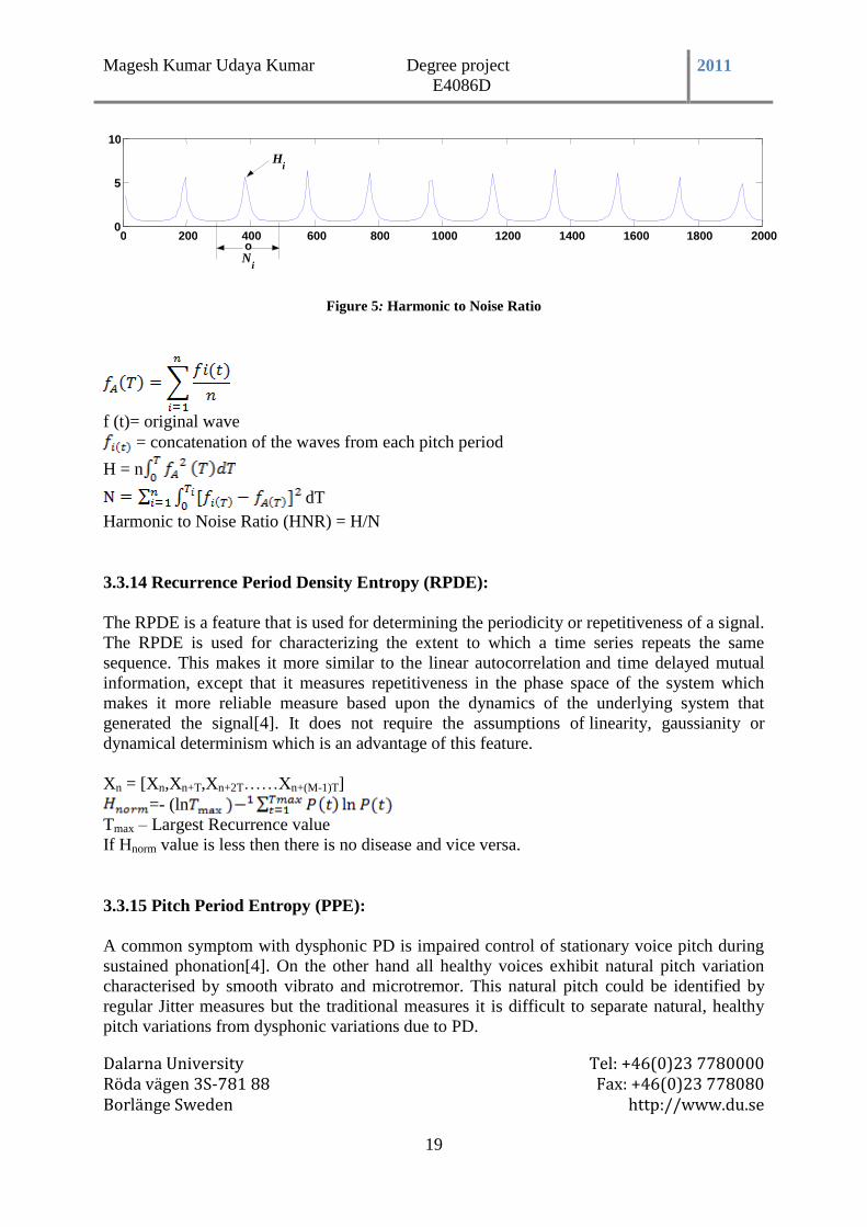
3.3.13 Harmonic to Noise Ratio (HNR):
The proportion of periodic and a-periodic waves in the vocal note is known as the Harmonics
to noise ratio. The vocal note produced by the vibrations of the vocal folds is complex and
made up of periodic that is regular and repetitive and aperiodic that is irregular and non-
repetitive sound waves. The aperiodic waves are random noise introduced into the vocal
signal owing to irregular or asymmetric adduction and it is necessary to identify the ratio of
both the waves[4]. PRAAT is capable of measuring the HNR and displaying the proportions.
For a signal that can be assumed periodic the signal-to-noise ratio equals the harmonics-to-
noise ratio. The greater the proportion of noise, the greater the perceived hoarseness, and the
lower the HNR Figure.
Magesh Kumar Udaya Kumar Degree project
E4086D 2011
Dalarna University Tel: +46(0)23 7780000 Röda vägen 3S-781 88 Fax: +46(0)23 778080 Borlänge Sweden http://www.du.se
19
Figure 5: Harmonic to Noise Ratio
f (t)= original wave
= concatenation of the waves from each pitch period
H = n
dT
Harmonic to Noise Ratio (HNR) = H/N
3.3.14 Recurrence Period Density Entropy (RPDE):
The RPDE is a feature that is used for determining the periodicity or repetitiveness of a signal.
The RPDE is used for characterizing the extent to which a time series repeats the same
sequence. This makes it more similar to the linear autocorrelation and time delayed mutual
information, except that it measures repetitiveness in the phase space of the system which
makes it more reliable measure based upon the dynamics of the underlying system that
generated the signal[4]. It does not require the assumptions of linearity, gaussianity or
dynamical determinism which is an advantage of this feature.
Xn = [Xn,Xn+T,Xn+2T……Xn+(M-1)T]
=- (ln
Tmax – Largest Recurrence value
If Hnorm value is less then there is no disease and vice versa.
3.3.15 Pitch Period Entropy (PPE):
A common symptom with dysphonic PD is impaired control of stationary voice pitch during
sustained phonation[4]. On the other hand all healthy voices exhibit natural pitch variation
characterised by smooth vibrato and microtremor. This natural pitch could be identified by
regular Jitter measures but the traditional measures it is difficult to separate natural, healthy
pitch variations from dysphonic variations due to PD.
0 200 400 600 800 1000 1200 1400 1600 1800 2000 0
5
10
H i
o N
i
Magesh Kumar Udaya Kumar Degree project
E4086D 2011
Dalarna University Tel: +46(0)23 7780000 Röda vägen 3S-781 88 Fax: +46(0)23 778080 Borlänge Sweden http://www.du.se
20
This could be overcome by implementing the following two insights.
1. The observations suggest that a more relevant scale on which to assess abnormal variations
in speech pitch is the perceptually-relevant logarithmic scale rather than the absolute
frequency scale.
2. In order to better capture pitch period variation due to PD related dysphonia independent of
these natural variations, smooth variations should be removed prior to measuring the extent of
such variations.
Now we can implement this algorithmically and calculate the entropy of probability
distribution. An increase in this entropy measure reflects better the variations over and above
natural healthy variations in pitch observed in healthy speech production.
3.3.16 Noise to Harmonic Ratio (NHR):
Noise to Harmonic Ratio (NHR) is another useful measure of hoarseness. For a signal that is
assumed to be periodic.
f (t)= original wave
= concatenation of the waves from each pitch period
H = n
dT
= 10 log
Period is nothing but how long it takes for the signal to repeat.
Fundamental Frequency =
3.3.17 Average fundamental frequency (Fo):
Average fundamental frequency (F0) (i.e.) the average value of all extracted period to period
fundamental frequency values.
3.3.18 Lowest fundamental frequency (Flo):
The lowest fundamental frequency (Flo) (i.e.) the lowest of all extracted period to period
fundamental frequency values.
Magesh Kumar Udaya Kumar Degree project
E4086D 2011
Dalarna University Tel: +46(0)23 7780000 Röda vägen 3S-781 88 Fax: +46(0)23 778080 Borlänge Sweden http://www.du.se
21
3.3.19 Highest fundamental frequency (Fhi):
Period: The period is the time taken for one complete cycle of a repeating waveform.
Frequency: This is the number of cycles completed per second. The measurement unit for
frequency is the hertz.
F0=1/Period The maximum fundamental frequency (Fhi) (i.e.) the greatest of all extracted period to period
fundamental frequency values.
3.3.20 Correlation Dimension (D2):
The D2 which is the measure of the complexity of a deterministic system gives the number of
independent variables necessary to describe the systems behavior[4]. The correlation
dimension (D2) is calculated by first time-delay embedding the signal to recreate the phase
space of the nonlinear dynamical system that is proposed to generate the speech signal. In this
reconstructed phase space, a geometrically self-similar (fractal) object indicates complex
dynamics, which are implicated in dysphonia. We use the TISEAN implementation, Roughly
speaking, the idea behind certain quantifiers of dimensions is that the weight p( of a
typical -ball covering part of the invariant set scales with its diameter like p( D2, where
the value for D depends also on the precise way one defines the weight. Using the square of
the probability pi to find a point of the set inside the ball, the dimension is called the
correlation dimension D2, which is computed most efficiently by the correlation sum,
C (m, ) = ))
Where,
Sj – m-dimensional delay vectors
NPairs -
= heavy side step function.
On sufficiently small length scales and when the embedding dimension m exceeds the box-
dimension of the attractor,
C (m,) D2
Since one does not know the box-dimension a priori, one checks for convergence of the
estimated values of D2 in m.
3.3.21 Spread1:
Spread1 is the log of the variance of the whitened pitch periods, First I need to calculate
pseries then I will be using this to extract „F‟ then this is used to get PDX then I used PDX in
calculating Spread1 and Spread2.Inorder to find pseries we have a formula,
12*log2(x/127.09);
Magesh Kumar Udaya Kumar Degree project
E4086D 2011
Dalarna University Tel: +46(0)23 7780000 Röda vägen 3S-781 88 Fax: +46(0)23 778080 Borlänge Sweden http://www.du.se
22
The input „X‟ vector of pitch periods in Hertz, obtained using Praat's pitch extraction
algorithm, divided by 127.09 and finding log2 then multiplied by 12.Then once we get pseries
then to get „A‟ we calculate it by
a = arcov(pseries,2);
Here we use arcov() then filter function to get f using for loop, now we use
xbins = linspace(-4.3,2.7,60);
pdx = hist(f,xbins);
pdx = pdx/sum(pdx);
spread1 = log(var(f)); xbin and get pdx by using hist() then we divide pdx with total sum of pdx to get exact pdx
value.For Spread1 we use log on var(f)
3.3.22 Spread2:
Spread2 is the entropy (estimated using histograms) of the whitened pitch periods, The
function 'entropy' just calculates the Shannon entropy.
pdx = hist(pseries,linspace(-14,14,60));
pdx = pdx/sum(pdx);
spread2 = entropy(pdx)/log(length(pdx));
we have different line spacing so we need to get pdx with this line spacing the order is same
as we done for Spread1,once we get „PDX‟ we use the length of PDX with log() divide it by
Entropy(pdx) we get Spread2.
3.4 Related Work:
There are few AI techniques that have been tried for several purposes in Parkinson disease.
There are few listed below,
Some of the related work using AI techniques to predict the Parkinson disease based on the
audio data set is as follows:
In diagnosing Parkinson by using Artificial Neural Networks and Support Vector Machine.
The proposed methods based on ANNs and SVMs to aid the specialist in the diagnosis of PD
[5]. The proposal is to build a system using Artificial Neural Networks (ANNs) and Support
Vector Machines (SVMs). The usage of such classifiers would reinforce and complement the
diagnosis of the specialists and their methods in the diagnosis tasks [5]. These two classifiers,
which are widely used for pattern recognition, should provide a good generalization
performance in the diagnosis task. The results presented by these three methods (MLP and
SVM with the two kernel types) have both a high precision level of the confusion matrix
regarding the different measurement parameters accuracy, sensitivity, specificity, positive
predictive value of the ANN and SVM were very good[5].

Magesh Kumar Udaya Kumar Degree project
E4086D 2011
Dalarna University Tel: +46(0)23 7780000 Röda vägen 3S-781 88 Fax: +46(0)23 778080 Borlänge Sweden http://www.du.se
23
In Suitability of dysphonia measurements for telemonitoring of Parkinson's disease.This
method presents an assessment of the practical value of existing traditional and non-standard
measures for discriminating healthy people from people with Parkinson Disease (PD) by
detecting dysphonia[6]. It introduces a new measure of dysphonia, Pitch Period Entropy
(PPE), which is robust to many uncontrollable confounding effects including noisy acoustic
environments and normal, healthy variations in voice frequency[4]. Vocal impairment may
also be one of the earliest indicators for the onset of the illness, and the measurement of voice
is noninvasive and simple to administer. Thus, voice measurement to detect and track the
progression of symptoms of PD has drawn significant attention. Dysphonic symptoms
typically include reduced loudness, breathiness, roughness, decreased energy in the higher
parts of the harmonic spectrum, and exaggerated vocal tremor.
Neural network-based approach to discriminate healthy people from those with Parkinson's
disease.This technique deals with the application of some probabilistic neural network (PNN)
variants to discriminate between healthy people and people with Parkinson's disease. Three
PNN types are used in this classification process, related to the smoothing factor search:
incremental search (IS), Monte Carlo search (MCS) and hybrid search (HS)[7]. The aim of
this technique was to verify the effectiveness of the application of PNN to a medical dataset,
related to Parkinson's diseases. The results obtained applying PNN show the robustness of this
methodology, even the data is very varied [7]. There is no major difference between the three
techniques of searching the smoothing parameter, although the hybrid technique seems to
better perform.
Accurate Telemonitoring of Parkinson‟s disease Progression by Noninvasive Speech Tests.
Tracking Parkinson's disease (PD) symptom progression often uses the Unified Parkinson‟s
Disease Rating Scale (UPDRS), which requires the patient's presence in clinic, and time-
consuming physical examinations by trained medical staff. Although the dysphonia measures
have physiological interpretations, it is difficult to link self-perception and physiology[8]. In
ongoing research work attempt is to establish a more physiologically-based model, which will
explain the data-driven findings in this study in terms of the relevant physiological changes
that occur in PD [8].
Assessing disordered speech and voice in Parkinson‟s disease a telerehabilitation application.
The aim of this method is to investigate the validity and reliability of a telerehabilitation
application for assessing the speech and voice disorder associated with Parkinson‟s
disease[9]. The assessment protocol included perceptual measures of voice and motor
function, articulatory precision, speech intelligibility, and acoustic measures of vocal sound
pressure level, phonation time and pitch range. This concludes that the majority of
parameters, comparable levels of agreement were achieved between the two environments[9].
Online assessment of disordered speech and voice in Parkinson‟s disease appears to be valid
and reliable.
Magesh Kumar Udaya Kumar Degree project
E4086D 2011
Dalarna University Tel: +46(0)23 7780000 Röda vägen 3S-781 88 Fax: +46(0)23 778080 Borlänge Sweden http://www.du.se
24
3.5 Proposed System:
As the disease seems to be more vulnerable and very difficult to identify or diagnose in the
early stages, in this work an efficient and more reliable way of classifying Parkinson disease
based on the audio data set. In order to apply these techniques, features have been classified
for the measures of the audio data set. The instances of this audio dataset is reduced by using
Discrete Cosine Transform(DCT).If all the features are ready then selection of features is
performed, After selecting the features, the selected feature is given to Weka and apply
various algorithms namely Multipass LVQ, K-Star, Logistic Model Tree .So this is how PD is
classified in this paper.
3.6 Data Pre-processing:
After collecting data, import the selected data in EXCEL and transform to Comma Delimited
(CSV) format. Using JAVA command to convert the .CSV format to .arff format which can
be used in WEKA.
• Remove ID field
• Create several subfiles
– Containing all the attributes
– Containing most important arrributes (2-19-21)
– Containing important arrributes (4-6-9-12-17-18-19-21)
3.7 Feature Extraction:
In the case where a large input data has to be fed into an algorithm problems like redundancy
where the large size of data and the amount of repeated and unwanted data being a part of it is
high. To overcome this we go in for feature extraction. It is here that the transformation of the
input data into a set of features. The total input data will be transformed into a reduced
representation set of features. The other reasons for choosing to do feature extraction are that
it takes the classification algorithm which overfits the training sample and generalizes poorly
to new samples and a lot of computational power and enormous amount of memory for
analyzing a large number of variables.
Magesh Kumar Udaya Kumar Degree project
E4086D 2011
Dalarna University Tel: +46(0)23 7780000 Röda vägen 3S-781 88 Fax: +46(0)23 778080 Borlänge Sweden http://www.du.se
25
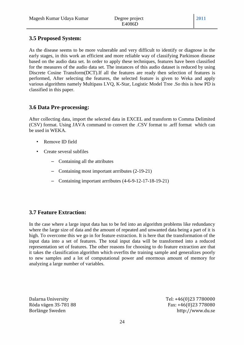
3.7.1 DCT:
The discrete cosine transform has been widely used in signal processing area usually in the 2-
dimensional domain because it has the power to compress information[10].
The Discrete Cosine Transform (DCT), like the Fourier Transform, converts a sequence of
samples to the frequency domain. But unlike the Fourier transform, the basis is made up of
cosine waves, therefore each basis wave has a set phase.
The DCT is to obtain significant features in a data set[11], a transform is usually applied,the
features are selected and then the inverse transform is applied. The most significant features
are the ones with the greatest variance. As shown, the KLT transforms a set of vectors, so that
each component of the vector represents the direction of greatest variance in decreasing order.
Therefore KLT is optimal for this task. We have seen that the DCT is a good approximation
to the KLT for first order stationaryMarkov processes. Therefore the DCT should be a good
Choice for transforming to a space for easy feature selection.
The first main advantage of the DCT is its efficiency[12]. As the size of the data to be
produced increases, the FFT becomes increasingly complex at a much more rapid rate, and is
not efficient for compression
Another advantage of the DCT is that its basis vectors are comprised of entirely real-valued
components.In Fourier analysis, one of the disadvantages is that every data affects every other
data, but if the DCT is used instead of the DFT, values of the data comes directly from the
transform of the time domain value.The DCT is similar to the discrete Fourier transform, it
transforms a signal from the spatial domain to the frequency domain[13].
X-axis - Actual Input
Y-axis - Output
Figure 6: Discrete Fourier Transform
Magesh Kumar Udaya Kumar Degree project
E4086D 2011
Dalarna University Tel: +46(0)23 7780000 Röda vägen 3S-781 88 Fax: +46(0)23 778080 Borlänge Sweden http://www.du.se
26
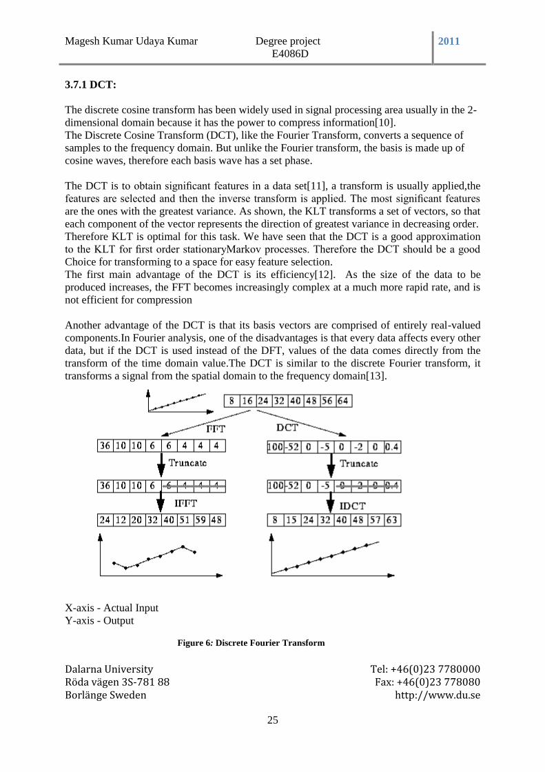
3.8 Visualizing all the attributes
The main GUI will show a histogram for the attribute distributions for a single selected
attribute at a time, by default this is the class attribute. Note that the individual colors indicate
the individual classes.
In the above table X-axis denotes the feature values. The feature value ranges according to the
respective feature range. These ranges are split using mean value. Y-axis denotes the number
of people lie in-between that range.
Figure 7: Visualizing all the Attributes
The table listed earlier is displayed diagrammatically here where the values of the attributes
are shown as results of weka. The visualization clearly explains the value of each attribute
along with its range of the value that the attribute gives. All the 23 attributes used are
mentioned here.

Magesh Kumar Udaya Kumar Degree project
E4086D 2011
Dalarna University Tel: +46(0)23 7780000 Röda vägen 3S-781 88 Fax: +46(0)23 778080 Borlänge Sweden http://www.du.se
27
3.9 Attribute Selection
There are lots of inbuilt methods in Weka to select the attributes, namely Chi squared,
Gain Ratio, Info Gain attribute evaluator to select the attributes and the results are shown
below:
3.9.1 Chi squared Attribute Evaluation
The chi-square statistic is a nonparametric statistical technique used to determine if a
distribution of observed values differs from the theoretical expected values. Chi-square
statistics use nominal (categorical) or ordinal level data, thus instead of using means and
variances. The value of the chi-square statistic is given by
X2 = Sigma [(O-E) 2 / E]
Where X2 is the chi-square statistic, O is the observed value and E is the expected value.
Table 4: Chi squared
X2 Feature Numbers Features
17.2117 6 DCT_RAP
13.6284 20 DCT_Spread2
13.0932 13 DCT_APQ
13.0932 22 DCT_PPE
13.0932 19 DCT_Spread1
8.8798 12 DCT_APQ5
8.8798 9 DCT_Shimmer
8.8798 11 DCT_APQ3
8.8798 10 DCT_ShimmerdB
8.8798 14 DCT_DDA
0 4 DCT_Jitter
0 21 DCT_D2
0 5 DCT_JitterAbs
0 1 DCT_Fo
0 3 DCT_Flo
0 2 DCT_Fhi
0 17 DCT_RPDE
0 15 DCT_NHR
0 16 DCT_HNR
0 7 DCT_PPQ
0 18 DCT_DFA
0 8 DCT_DDP
Magesh Kumar Udaya Kumar Degree project
E4086D 2011
Dalarna University Tel: +46(0)23 7780000 Röda vägen 3S-781 88 Fax: +46(0)23 778080 Borlänge Sweden http://www.du.se
28
Chisquared attribute evaluation is a built in evaluation feature that is used to evaluate the
attributes and rank them as per the priority of order. The given chisquared attribute evaluation
gives the result of attributes listed above as the best attributes for evaluation.
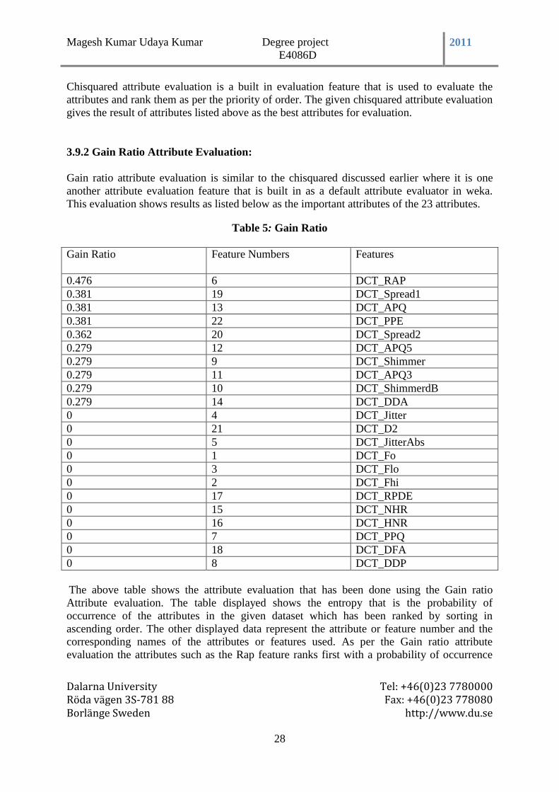
3.9.2 Gain Ratio Attribute Evaluation:
Gain ratio attribute evaluation is similar to the chisquared discussed earlier where it is one
another attribute evaluation feature that is built in as a default attribute evaluator in weka.
This evaluation shows results as listed below as the important attributes of the 23 attributes.
Table 5: Gain Ratio
Gain Ratio Feature Numbers Features
0.476 6 DCT_RAP
0.381 19 DCT_Spread1
0.381 13 DCT_APQ
0.381 22 DCT_PPE
0.362 20 DCT_Spread2
0.279 12 DCT_APQ5
0.279 9 DCT_Shimmer
0.279 11 DCT_APQ3
0.279 10 DCT_ShimmerdB
0.279 14 DCT_DDA
0 4 DCT_Jitter
0 21 DCT_D2
0 5 DCT_JitterAbs
0 1 DCT_Fo
0 3 DCT_Flo
0 2 DCT_Fhi
0 17 DCT_RPDE
0 15 DCT_NHR
0 16 DCT_HNR
0 7 DCT_PPQ
0 18 DCT_DFA
0 8 DCT_DDP
The above table shows the attribute evaluation that has been done using the Gain ratio
Attribute evaluation. The table displayed shows the entropy that is the probability of
occurrence of the attributes in the given dataset which has been ranked by sorting in
ascending order. The other displayed data represent the attribute or feature number and the
corresponding names of the attributes or features used. As per the Gain ratio attribute
evaluation the attributes such as the Rap feature ranks first with a probability of occurrence
Magesh Kumar Udaya Kumar Degree project
E4086D 2011
Dalarna University Tel: +46(0)23 7780000 Röda vägen 3S-781 88 Fax: +46(0)23 778080 Borlänge Sweden http://www.du.se
29
value of 0.476. Similarly the other features with high probability are the Spread1, APQ, PPE
and a few others in the given sorted order.
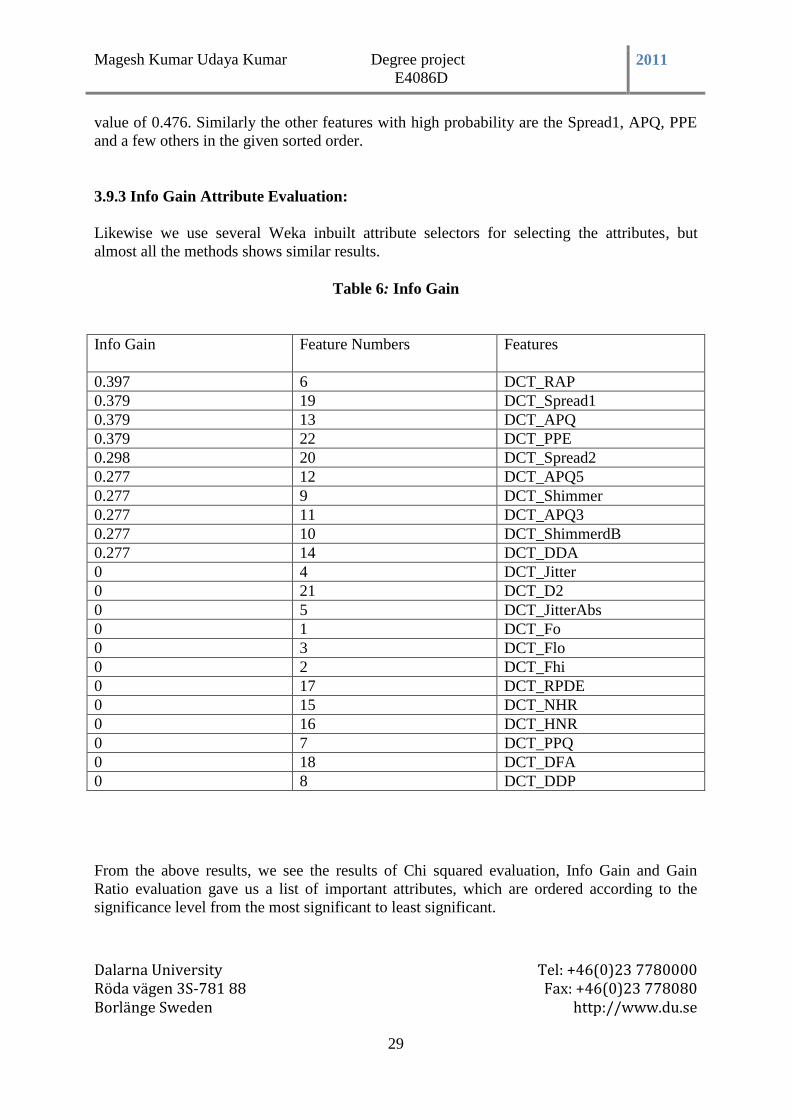
3.9.3 Info Gain Attribute Evaluation:
Likewise we use several Weka inbuilt attribute selectors for selecting the attributes, but
almost all the methods shows similar results.
Table 6: Info Gain
Info Gain Feature Numbers Features
0.397 6 DCT_RAP
0.379 19 DCT_Spread1
0.379 13 DCT_APQ
0.379 22 DCT_PPE
0.298 20 DCT_Spread2
0.277 12 DCT_APQ5
0.277 9 DCT_Shimmer
0.277 11 DCT_APQ3
0.277 10 DCT_ShimmerdB
0.277 14 DCT_DDA
0 4 DCT_Jitter
0 21 DCT_D2
0 5 DCT_JitterAbs
0 1 DCT_Fo
0 3 DCT_Flo
0 2 DCT_Fhi
0 17 DCT_RPDE
0 15 DCT_NHR
0 16 DCT_HNR
0 7 DCT_PPQ
0 18 DCT_DFA
0 8 DCT_DDP
From the above results, we see the results of Chi squared evaluation, Info Gain and Gain
Ratio evaluation gave us a list of important attributes, which are ordered according to the
significance level from the most significant to least significant.
Magesh Kumar Udaya Kumar Degree project
E4086D 2011
Dalarna University Tel: +46(0)23 7780000 Röda vägen 3S-781 88 Fax: +46(0)23 778080 Borlänge Sweden http://www.du.se
30
Although the list gave information of the attribute significance, but based on only that we
cannot able to select the attributes.
The above table shows the attribute evaluation that has been done using the Info Gain
Attribute evaluation. The table displayed shows the entropy that is the probability of
occurrence of the attributes in the given dataset which has been ranked by sorting in
ascending order. The other displayed data represent the attribute or feature number and the
corresponding names of the attributes or features used. As per the Info Gain attribute
evaluation the attributes such as the Rap feature ranks first in this case as well similar to the
previous attribute selector, with a probability of occurrence value of 0.397. Similarly the other
features with high probability are the Spread1, APQ, PPE and a few others in the given sorted
order.
3.9.4 Stepwise Regression:
In order to select the important attributes, we need to analyse the structure of this data set
using Minitab statistical software, Stepwise Regression is a useful approach for selecting the
attributes one by one.
From the above methods, we combine all the results of the Weka build in methods and get the
result: DCT_RAP, DCT_spread2, DCT_APQ, DCT_PPE, DCT_spread1, DCT_APQ5,
DCT_Shimmer, DCT_APQ3, DCT_ShimmerdB, and DCT_DDA.The rest of the features
which we will check in the further analysis.
Justification of the selected features:
First step we give the response i.e. “Status” and give the predictors i.e. all the attributes but
we do not set any predictors to include in every model. The result is shown below,
T-value: Indicates the Significance of each component in improving the regression equation.
P-value: The p-value measures consistency between the results actually obtained in the trial
and the ”pure chance" explanation for those results
S-value: It gives the standard deviation of the residuals.
R-Sq: It is a statistic that will give some information about the goodness of fit of a model. In
regression, the R2 coefficient of determination is a statistical measure of how well the
regression line approximates the real data points. An R2 of 100.0 indicates that the regression
line perfectly fits the data.
R-Sq(adj): Adjusted R2 is a modification of R
2 that adjusts for the number of explanatory
terms in a model. Unlike R2 , the adjusted R
2 increases only if the new term improves the
model more than would be expected by chance. The adjusted R2 can be negative, and will
always be less than or equal to R2 .
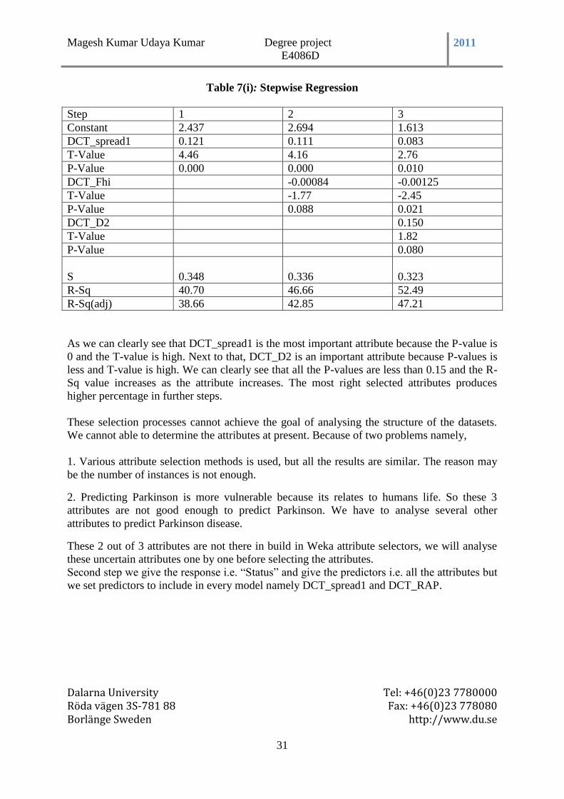
Magesh Kumar Udaya Kumar Degree project
E4086D 2011
Dalarna University Tel: +46(0)23 7780000 Röda vägen 3S-781 88 Fax: +46(0)23 778080 Borlänge Sweden http://www.du.se
31
Table 7(i): Stepwise Regression
Step 1 2 3
Constant 2.437 2.694 1.613
DCT_spread1 0.121 0.111 0.083
T-Value 4.46 4.16 2.76
P-Value 0.000 0.000 0.010
DCT_Fhi -0.00084 -0.00125
T-Value -1.77 -2.45
P-Value 0.088 0.021
DCT_D2 0.150
T-Value 1.82
P-Value 0.080
S
0.348
0.336
0.323
R-Sq 40.70 46.66 52.49
R-Sq(adj) 38.66 42.85 47.21
As we can clearly see that DCT_spread1 is the most important attribute because the P-value is
0 and the T-value is high. Next to that, DCT_D2 is an important attribute because P-values is
less and T-value is high. We can clearly see that all the P-values are less than 0.15 and the R-
Sq value increases as the attribute increases. The most right selected attributes produces
higher percentage in further steps.
These selection processes cannot achieve the goal of analysing the structure of the datasets.
We cannot able to determine the attributes at present. Because of two problems namely,
1. Various attribute selection methods is used, but all the results are similar. The reason may
be the number of instances is not enough.
2. Predicting Parkinson is more vulnerable because its relates to humans life. So these 3
attributes are not good enough to predict Parkinson. We have to analyse several other
attributes to predict Parkinson disease.
These 2 out of 3 attributes are not there in build in Weka attribute selectors, we will analyse
these uncertain attributes one by one before selecting the attributes.
Second step we give the response i.e. “Status” and give the predictors i.e. all the attributes but
we set predictors to include in every model namely DCT_spread1 and DCT_RAP.
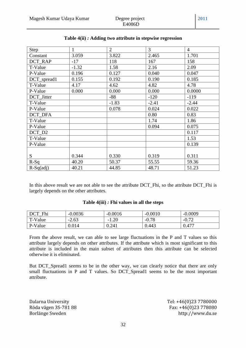
Magesh Kumar Udaya Kumar Degree project
E4086D 2011
Dalarna University Tel: +46(0)23 7780000 Röda vägen 3S-781 88 Fax: +46(0)23 778080 Borlänge Sweden http://www.du.se
32
Table 4(ii) : Adding two attribute in stepwise regression
Step 1 2 3 4
Constant 3.059 3.822 2.465 1.701
DCT_RAP -17 118 167 158
T-Value -1.32 1.58 2.16 2.09
P-Value 0.196 0.127 0.040 0.047
DCT_spread1 0.155 0.192 0.190 0.185
T-Value 4.17 4.62 4.82 4.78
P-Value 0.000 0.000 0.000 0.0000
DCT_Jitter -88 -120 -119
T-Value -1.83 -2.41 -2.44
P-Value 0.078 0.024 0.022
DCT_DFA 0.80 0.83
T-Value 1.74 1.86
P-Value 0.094 0.075
DCT_D2 0.117
T-Value 1.53
P-Value 0.139
S
0.344
0.330
0.319
0.311
R-Sq 40.20 50.37 55.55 59.36
R-Sq(adj) 40.21 44.85 48.71 51.23
In this above result we are not able to see the attribute DCT_Fhi, so the attribute DCT_Fhi is
largely depends on the other attributes.
Table 4(iii) : Fhi values in all the steps
DCT_Fhi -0.0036 -0.0016 -0.0010 -0.0009
T-Value -2.63 -1.20 -0.78 -0.72
P-Value 0.014 0.241 0.443 0.477
From the above result, we can able to see large fluctuations in the P and T values so this
attribute largely depends on other attributes. If the attribute which is most significant to this
attribute is included in the main subset of attributes then this attribute can be selected
otherwise it is eliminated.
But DCT_Spread1 seems to be in the other way, we can clearly notice that there are only
small fluctuations in P and T values. So DCT_Spread1 seems to be the most important
attribute.
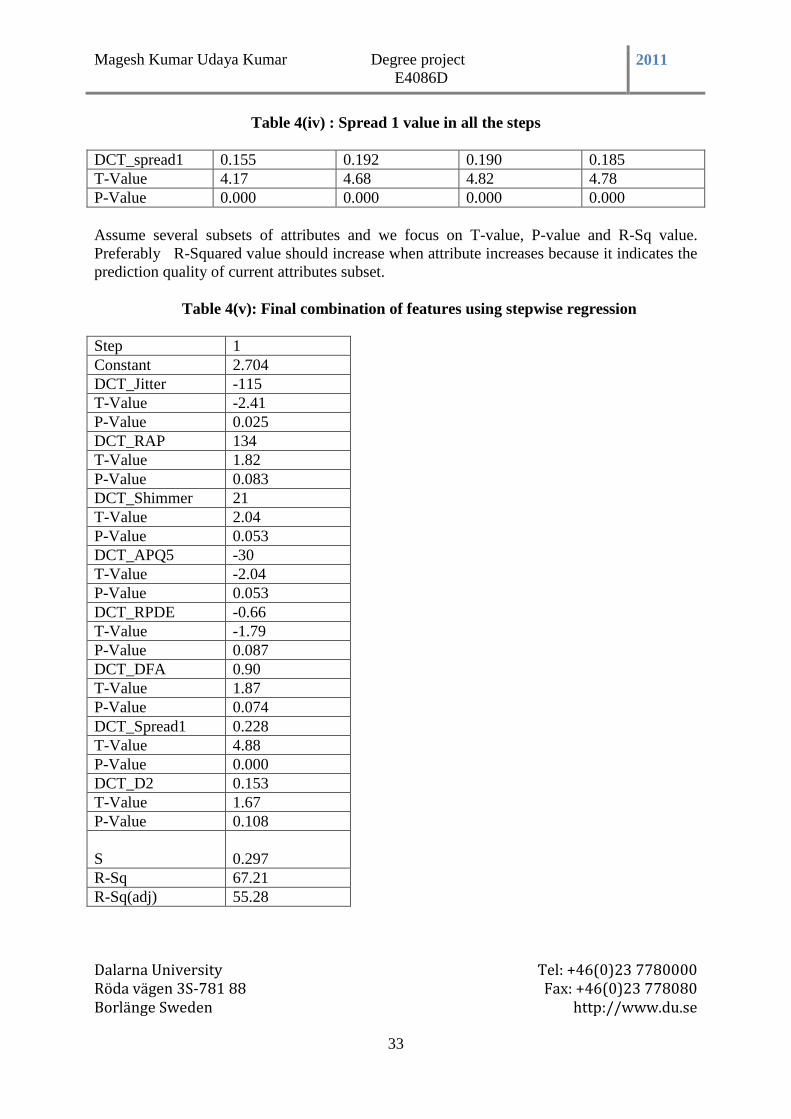
Magesh Kumar Udaya Kumar Degree project
E4086D 2011
Dalarna University Tel: +46(0)23 7780000 Röda vägen 3S-781 88 Fax: +46(0)23 778080 Borlänge Sweden http://www.du.se
33
Table 4(iv) : Spread 1 value in all the steps
DCT_spread1 0.155 0.192 0.190 0.185
T-Value 4.17 4.68 4.82 4.78
P-Value 0.000 0.000 0.000 0.000
Assume several subsets of attributes and we focus on T-value, P-value and R-Sq value.
Preferably R-Squared value should increase when attribute increases because it indicates the
prediction quality of current attributes subset.
Table 4(v): Final combination of features using stepwise regression
Step 1
Constant 2.704
DCT_Jitter -115
T-Value -2.41
P-Value 0.025
DCT_RAP 134
T-Value 1.82
P-Value 0.083
DCT_Shimmer 21
T-Value 2.04
P-Value 0.053
DCT_APQ5 -30
T-Value -2.04
P-Value 0.053
DCT_RPDE -0.66
T-Value -1.79
P-Value 0.087
DCT_DFA 0.90
T-Value 1.87
P-Value 0.074
DCT_Spread1 0.228
T-Value 4.88
P-Value 0.000
DCT_D2 0.153
T-Value 1.67
P-Value 0.108
S
0.297
R-Sq 67.21
R-Sq(adj) 55.28
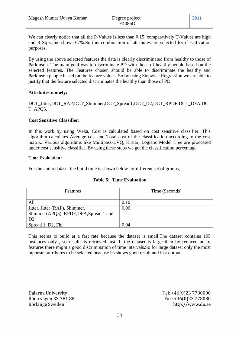
Magesh Kumar Udaya Kumar Degree project
E4086D 2011
Dalarna University Tel: +46(0)23 7780000 Röda vägen 3S-781 88 Fax: +46(0)23 778080 Borlänge Sweden http://www.du.se
34
We can clearly notice that all the P-Values is less than 0.15, comparatively T-Values are high
and R-Sq value shows 67%.So this combination of attributes are selected for classification
purposes.
By using the above selected features the data is clearly discriminated from healthy to those of
Parkinson. The main goal was to discriminate PD with those of healthy people based on the
selected features. The Features chosen should be able to discriminate the healthy and
Parkinson people based on the feature values. So by using Stepwise Regression we are able to
justify that the feature selected discriminates the healthy than those of PD.
Attributes namely:
DCT_Jitter,DCT_RAP,DCT_Shimmer,DCT_Spread1,DCT_D2,DCT_RPDE,DCT_DFA,DC
T_APQ5.
Cost Sensitive Classifier:
In this work by using Weka, Cost is calculated based on cost sensitive classifier. This
algorithm calculates Average cost and Total cost of the classification according to the cost
matrix. Various algorithms like Multipass-LVQ, K star, Logistic Model Tree are processed
under cost sensitive classifier. By using these steps we get the classification percentage.
Time Evaluation :
For the audio dataset the build time is shown below for different set of groups,
Table 5: Time Evaluation
Features
Time (Seconds)
All 0.10
Jitter, Jitter (RAP), Shimmer,
Shimmer(APQ5), RPDE,DFA,Spread 1 and
D2
0.06
Spread 1, D2, Fhi 0.04
This seems to build at a fast rate because the dataset is small.The dataset contains 195
instances only , so results is retrieved fast .If the dataset is large then by reduced no of
features there might a good discrimination of time intervals.So for large dataset only the most
inportant attributes to be selected beacuse its shows good result and fast output.
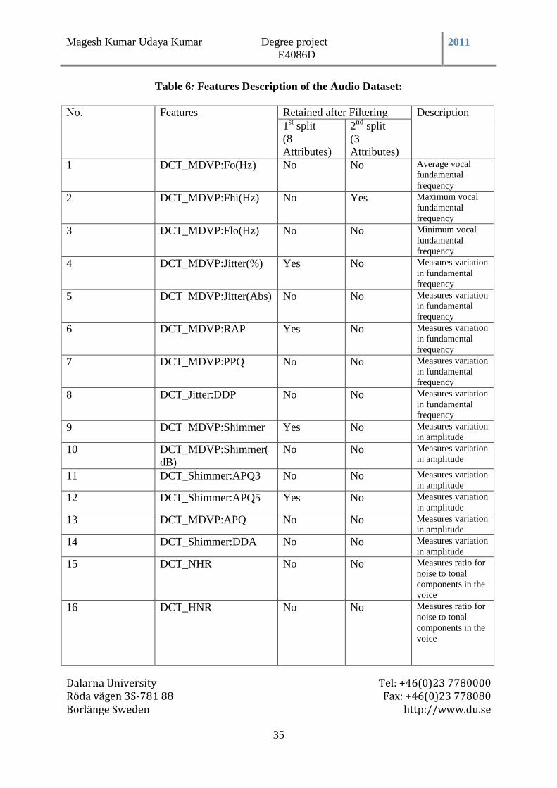
Magesh Kumar Udaya Kumar Degree project
E4086D 2011
Dalarna University Tel: +46(0)23 7780000 Röda vägen 3S-781 88 Fax: +46(0)23 778080 Borlänge Sweden http://www.du.se
35
Table 6: Features Description of the Audio Dataset:
No. Features Retained after Filtering Description
1st split
(8
Attributes)
2nd
split
(3
Attributes)
1 DCT_MDVP:Fo(Hz) No No Average vocal
fundamental
frequency
2 DCT_MDVP:Fhi(Hz) No Yes Maximum vocal
fundamental
frequency
3 DCT_MDVP:Flo(Hz) No No Minimum vocal
fundamental
frequency
4 DCT_MDVP:Jitter(%) Yes No Measures variation
in fundamental
frequency
5 DCT_MDVP:Jitter(Abs) No No Measures variation
in fundamental
frequency
6 DCT_MDVP:RAP Yes No Measures variation
in fundamental
frequency
7 DCT_MDVP:PPQ No No Measures variation
in fundamental
frequency
8 DCT_Jitter:DDP No No Measures variation
in fundamental
frequency
9 DCT_MDVP:Shimmer Yes No Measures variation
in amplitude
10 DCT_MDVP:Shimmer(
dB)
No No Measures variation
in amplitude
11 DCT_Shimmer:APQ3 No No Measures variation
in amplitude
12 DCT_Shimmer:APQ5 Yes No Measures variation
in amplitude
13 DCT_MDVP:APQ No No Measures variation
in amplitude
14 DCT_Shimmer:DDA No No Measures variation
in amplitude
15 DCT_NHR No No Measures ratio for
noise to tonal
components in the
voice
16 DCT_HNR No No Measures ratio for
noise to tonal
components in the
voice
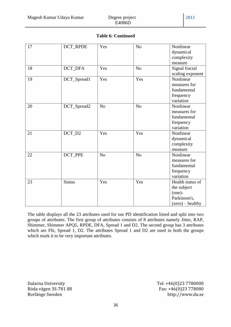
Magesh Kumar Udaya Kumar Degree project
E4086D 2011
Dalarna University Tel: +46(0)23 7780000 Röda vägen 3S-781 88 Fax: +46(0)23 778080 Borlänge Sweden http://www.du.se
36
Table 6: Continued
17 DCT_RPDE Yes No Nonlinear
dynamical
complexity
measure
18 DCT_DFA Yes No Signal fractal
scaling exponent
19 DCT_Spread1 Yes Yes Nonlinear
measures for
fundamental
frequency
variation
20 DCT_Spread2 No No Nonlinear
measures for
fundamental
frequency
variation
21 DCT_D2 Yes Yes Nonlinear
dynamical
complexity
measure
22 DCT_PPE No No Nonlinear
measures for
fundamental
frequency
variation
23 Status Yes Yes Health status of
the subject
(one)-
Parkinson's,
(zero) – healthy
The table displays all the 23 attributes used for our PD identification listed and split into two
groups of attributes. The first group of attributes consists of 8 attributes namely Jitter, RAP,
Shimmer, Shimmer APQ5, RPDE, DFA, Spread 1 and D2. The second group has 3 attributes
which are Fhi, Spread 1, D2. The attributes Spread 1 and D2 are used in both the groups
which mark it to be very important attributes.
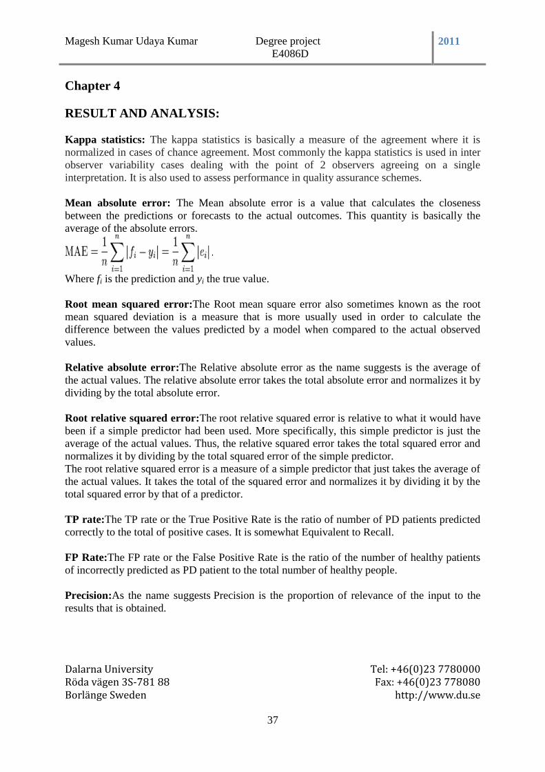
Magesh Kumar Udaya Kumar Degree project
E4086D 2011
Dalarna University Tel: +46(0)23 7780000 Röda vägen 3S-781 88 Fax: +46(0)23 778080 Borlänge Sweden http://www.du.se
37
Chapter 4
RESULT AND ANALYSIS:
Kappa statistics: The kappa statistics is basically a measure of the agreement where it is
normalized in cases of chance agreement. Most commonly the kappa statistics is used in inter
observer variability cases dealing with the point of 2 observers agreeing on a single
interpretation. It is also used to assess performance in quality assurance schemes.
Mean absolute error: The Mean absolute error is a value that calculates the closeness
between the predictions or forecasts to the actual outcomes. This quantity is basically the
average of the absolute errors.
Where fi is the prediction and yi the true value.
Root mean squared error:The Root mean square error also sometimes known as the root
mean squared deviation is a measure that is more usually used in order to calculate the
difference between the values predicted by a model when compared to the actual observed
values.
Relative absolute error:The Relative absolute error as the name suggests is the average of
the actual values. The relative absolute error takes the total absolute error and normalizes it by
dividing by the total absolute error.
Root relative squared error:The root relative squared error is relative to what it would have
been if a simple predictor had been used. More specifically, this simple predictor is just the
average of the actual values. Thus, the relative squared error takes the total squared error and
normalizes it by dividing by the total squared error of the simple predictor.
The root relative squared error is a measure of a simple predictor that just takes the average of
the actual values. It takes the total of the squared error and normalizes it by dividing it by the
total squared error by that of a predictor.
TP rate:The TP rate or the True Positive Rate is the ratio of number of PD patients predicted
correctly to the total of positive cases. It is somewhat Equivalent to Recall.
FP Rate:The FP rate or the False Positive Rate is the ratio of the number of healthy patients
of incorrectly predicted as PD patient to the total number of healthy people.
Precision:As the name suggests Precision is the proportion of relevance of the input to the
results that is obtained.
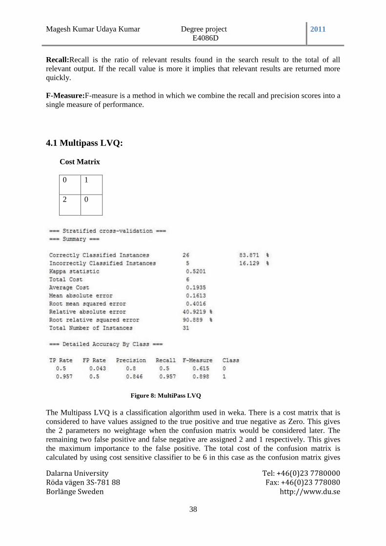
Magesh Kumar Udaya Kumar Degree project
E4086D 2011
Dalarna University Tel: +46(0)23 7780000 Röda vägen 3S-781 88 Fax: +46(0)23 778080 Borlänge Sweden http://www.du.se
38
Recall:Recall is the ratio of relevant results found in the search result to the total of all
relevant output. If the recall value is more it implies that relevant results are returned more
quickly.
F-Measure:F-measure is a method in which we combine the recall and precision scores into a
single measure of performance.
4.1 Multipass LVQ:
Cost Matrix
0 1
2 0
Figure 8: MultiPass LVQ
The Multipass LVQ is a classification algorithm used in weka. There is a cost matrix that is
considered to have values assigned to the true positive and true negative as Zero. This gives
the 2 parameters no weightage when the confusion matrix would be considered later. The
remaining two false positive and false negative are assigned 2 and 1 respectively. This gives
the maximum importance to the false positive. The total cost of the confusion matrix is
calculated by using cost sensitive classifier to be 6 in this case as the confusion matrix gives
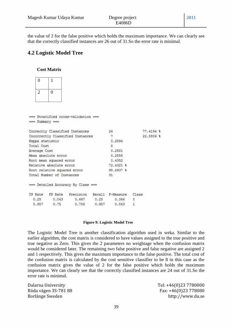
Magesh Kumar Udaya Kumar Degree project
E4086D 2011
Dalarna University Tel: +46(0)23 7780000 Röda vägen 3S-781 88 Fax: +46(0)23 778080 Borlänge Sweden http://www.du.se
39
the value of 2 for the false positive which holds the maximum importance. We can clearly see
that the correctly classified instances are 26 out of 31.So the error rate is minimal.
4.2 Logistic Model Tree
Cost Matrix
0 1
2 0
Figure 9: Logistic Model Tree
The Logistic Model Tree is another classification algorithm used in weka. Similar to the
earlier algorithm, the cost matrix is considered to have values assigned to the true positive and
true negative as Zero. This gives the 2 parameters no weightage when the confusion matrix
would be considered later. The remaining two false positive and false negative are assigned 2
and 1 respectively. This gives the maximum importance to the false positive. The total cost of
the confusion matrix is calculated by the cost sensitive classifier to be 8 in this case as the
confusion matrix gives the value of 2 for the false positive which holds the maximum
importance. We can clearly see that the correctly classified instances are 24 out of 31.So the
error rate is minimal.
Magesh Kumar Udaya Kumar Degree project
E4086D 2011
Dalarna University Tel: +46(0)23 7780000 Röda vägen 3S-781 88 Fax: +46(0)23 778080 Borlänge Sweden http://www.du.se
40
4.3 K-Star Algorithm
Cost Matrix
0 1
2 0
Figure 10: K-Star Algorithm
The K* Algorithm is another classification algorithm used in weka. Similar to the earlier
algorithms, the cost matrix is has values assigned to the true positive and true negative as
Zero. This gives the 2 parameters no weightage when the confusion matrix would be
considered later. The remaining two false positive and false negative are assigned 2 and 1
respectively. This gives the maximum importance to the false positive. The total cost of the
confusion matrix is calculated by the cost sensitive classifier to be 6 in this case as the
confusion matrix gives the value of 2 for the false positive which holds the maximum
importance. We can clearly see that the correctly classified instances are 25 out of 31.So the
error rate is minimal.
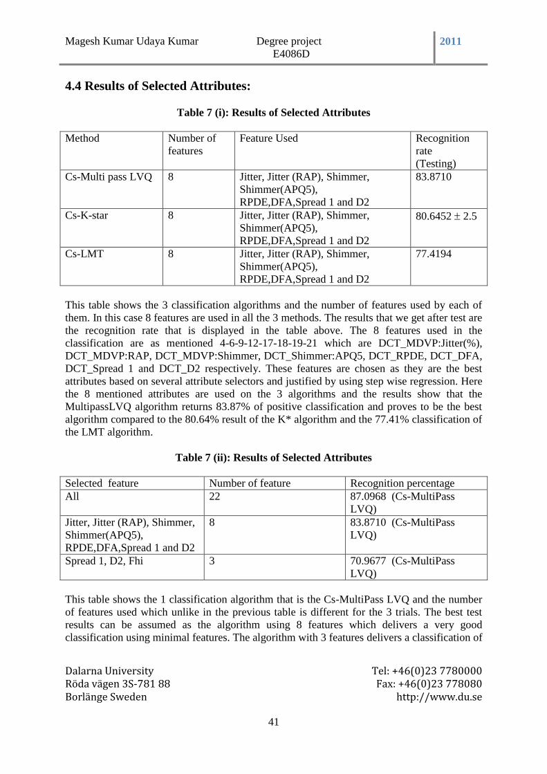
Magesh Kumar Udaya Kumar Degree project
E4086D 2011
Dalarna University Tel: +46(0)23 7780000 Röda vägen 3S-781 88 Fax: +46(0)23 778080 Borlänge Sweden http://www.du.se
41
4.4 Results of Selected Attributes:
Table 7 (i): Results of Selected Attributes
Method Number of
features
Feature Used Recognition
rate
(Testing)
Cs-Multi pass LVQ 8 Jitter, Jitter (RAP), Shimmer,
Shimmer(APQ5),
RPDE,DFA,Spread 1 and D2
83.8710
Cs-K-star 8 Jitter, Jitter (RAP), Shimmer,
Shimmer(APQ5),
RPDE,DFA,Spread 1 and D2
80.6452 2.5
Cs-LMT 8 Jitter, Jitter (RAP), Shimmer,
Shimmer(APQ5),
RPDE,DFA,Spread 1 and D2
77.4194
This table shows the 3 classification algorithms and the number of features used by each of
them. In this case 8 features are used in all the 3 methods. The results that we get after test are
the recognition rate that is displayed in the table above. The 8 features used in the
classification are as mentioned 4-6-9-12-17-18-19-21 which are DCT_MDVP:Jitter(%),
DCT_MDVP:RAP, DCT_MDVP:Shimmer, DCT_Shimmer:APQ5, DCT_RPDE, DCT_DFA,
DCT_Spread 1 and DCT_D2 respectively. These features are chosen as they are the best
attributes based on several attribute selectors and justified by using step wise regression. Here
the 8 mentioned attributes are used on the 3 algorithms and the results show that the
MultipassLVQ algorithm returns 83.87% of positive classification and proves to be the best
algorithm compared to the 80.64% result of the K* algorithm and the 77.41% classification of
the LMT algorithm.
Table 7 (ii): Results of Selected Attributes
Selected feature Number of feature Recognition percentage
All 22 87.0968 (Cs-MultiPass
LVQ)
Jitter, Jitter (RAP), Shimmer,
Shimmer(APQ5),
RPDE,DFA,Spread 1 and D2
8 83.8710 (Cs-MultiPass
LVQ)
Spread 1, D2, Fhi 3 70.9677 (Cs-MultiPass
LVQ)
This table shows the 1 classification algorithm that is the Cs-MultiPass LVQ and the number
of features used which unlike in the previous table is different for the 3 trials. The best test
results can be assumed as the algorithm using 8 features which delivers a very good
classification using minimal features. The algorithm with 3 features delivers a classification of
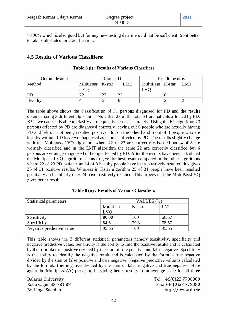
Magesh Kumar Udaya Kumar Degree project
E4086D 2011
Dalarna University Tel: +46(0)23 7780000 Röda vägen 3S-781 88 Fax: +46(0)23 778080 Borlänge Sweden http://www.du.se
42
70.96% which is also good but for any new testing data it would not be sufficient. So it better
to take 8 attributes for classification.
4.5 Results of Various Classifiers:
Table 8 (i) : Results of Various Classifiers
Output desired Result PD Result healthy
Method MultiPass
LVQ
K-star LMT MultiPass
LVQ
K-star LMT
PD 22 23 22 1 0 1
Healthy 4 6 6 4 2 2
The table above shows the classification of 31 persons diagnosed for PD and the results
obtained using 3 different algorithms. Note that 23 of the total 31 are patients affected by PD.
K*as we can see is able to clasify all the positive cases accurately. Using the K* algorithm 23
persons affected by PD are diagnosed correctly leaving out 0 people who are actually having
PD and left out not being resulted positive. But on the other hand 6 out of 8 people who are
healthy without PD have we diagnosed as patients affected by PD. The results slightly change
with the Multipass LVQ algorithm where 22 of 23 are correctly calssified and 4 of 8 are
worngly classified and in the LMT algorithm the same 22 are correctly classified but 6
persons are wrongly diagnosed of being affected by PD. After the results have been calculated
the Multipass LVQ algorithm seems to give the best result compared to the other algorithms
where 22 of 23 PD patients and 4 of 8 healthy people have been positively resulted this gives
26 of 31 positive results. Whereas in Kstar algorithm 25 of 31 people have been resulted
positively and similarly only 24 have positively resulted. This proves that the MultiPassLVQ
gives better results.
Table 8 (ii) : Results of Various Classifiers
Statistical parameters VALUES (%)
MultiPass
LVQ
K-star LMT
Sensitivity 80.00 100 66.67
Specificity 84.61 79.31 78.57
Negative predictive value 95.65 100 95.65
This table shows the 3 different statistical parameters namely sensitivity, specificity and
negative predictive value. Sensitivity is the ability to find the positive results and is calculated
by the formula true positive divided by the sum of true positive and false negative. Specificity
is the ability to identify the negative result and is calculated by the formula true negative
divided by the sum of false positive and true negative. Negative predictive value is calculated
by the formula true negative divided by the sum of false negative and true negative. Here
again the MultipassLVQ proves to be giving better results in an average scale for all three
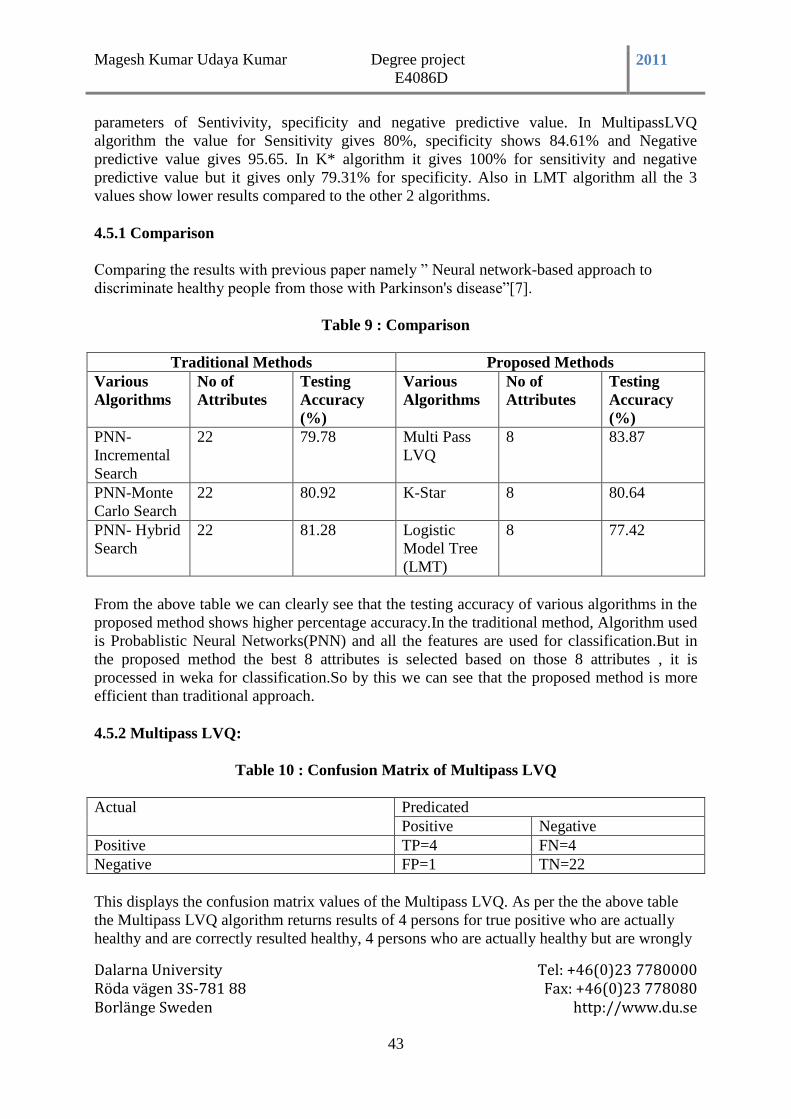
Magesh Kumar Udaya Kumar Degree project
E4086D 2011
Dalarna University Tel: +46(0)23 7780000 Röda vägen 3S-781 88 Fax: +46(0)23 778080 Borlänge Sweden http://www.du.se
43
parameters of Sentivivity, specificity and negative predictive value. In MultipassLVQ
algorithm the value for Sensitivity gives 80%, specificity shows 84.61% and Negative
predictive value gives 95.65. In K* algorithm it gives 100% for sensitivity and negative
predictive value but it gives only 79.31% for specificity. Also in LMT algorithm all the 3
values show lower results compared to the other 2 algorithms.
4.5.1 Comparison
Comparing the results with previous paper namely ” Neural network-based approach to
discriminate healthy people from those with Parkinson's disease”[7].
Table 9 : Comparison
Traditional Methods Proposed Methods
Various
Algorithms
No of
Attributes
Testing
Accuracy
(%)
Various
Algorithms
No of
Attributes
Testing
Accuracy
(%)
PNN-
Incremental
Search
22 79.78 Multi Pass
LVQ
8 83.87
PNN-Monte
Carlo Search
22 80.92 K-Star 8 80.64
PNN- Hybrid
Search
22 81.28 Logistic
Model Tree
(LMT)
8 77.42
From the above table we can clearly see that the testing accuracy of various algorithms in the
proposed method shows higher percentage accuracy.In the traditional method, Algorithm used
is Probablistic Neural Networks(PNN) and all the features are used for classification.But in
the proposed method the best 8 attributes is selected based on those 8 attributes , it is
processed in weka for classification.So by this we can see that the proposed method is more
efficient than traditional approach.
4.5.2 Multipass LVQ:
Table 10 : Confusion Matrix of Multipass LVQ
Actual Predicated
Positive Negative
Positive TP=4 FN=4
Negative FP=1 TN=22
This displays the confusion matrix values of the Multipass LVQ. As per the the above table
the Multipass LVQ algorithm returns results of 4 persons for true positive who are actually
healthy and are correctly resulted healthy, 4 persons who are actually healthy but are wrongly
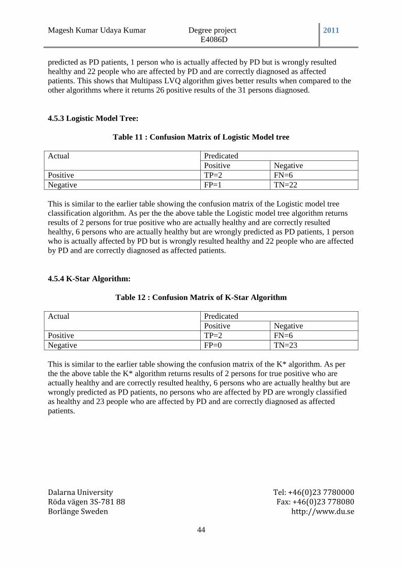
Magesh Kumar Udaya Kumar Degree project
E4086D 2011
Dalarna University Tel: +46(0)23 7780000 Röda vägen 3S-781 88 Fax: +46(0)23 778080 Borlänge Sweden http://www.du.se
44
predicted as PD patients, 1 person who is actually affected by PD but is wrongly resulted
healthy and 22 people who are affected by PD and are correctly diagnosed as affected
patients. This shows that Multipass LVQ algorithm gives better results when compared to the
other algorithms where it returns 26 positive results of the 31 persons diagnosed.
4.5.3 Logistic Model Tree:
Table 11 : Confusion Matrix of Logistic Model tree
Actual Predicated
Positive Negative
Positive TP=2 FN=6
Negative FP=1 TN=22
This is similar to the earlier table showing the confusion matrix of the Logistic model tree
classification algorithm. As per the the above table the Logistic model tree algorithm returns
results of 2 persons for true positive who are actually healthy and are correctly resulted
healthy, 6 persons who are actually healthy but are wrongly predicted as PD patients, 1 person
who is actually affected by PD but is wrongly resulted healthy and 22 people who are affected
by PD and are correctly diagnosed as affected patients.
4.5.4 K-Star Algorithm:
Table 12 : Confusion Matrix of K-Star Algorithm
Actual Predicated
Positive Negative
Positive TP=2 FN=6
Negative FP=0 TN=23
This is similar to the earlier table showing the confusion matrix of the K* algorithm. As per
the the above table the K* algorithm returns results of 2 persons for true positive who are
actually healthy and are correctly resulted healthy, 6 persons who are actually healthy but are
wrongly predicted as PD patients, no persons who are affected by PD are wrongly classified
as healthy and 23 people who are affected by PD and are correctly diagnosed as affected
patients.
Magesh Kumar Udaya Kumar Degree project
E4086D 2011
Dalarna University Tel: +46(0)23 7780000 Röda vägen 3S-781 88 Fax: +46(0)23 778080 Borlänge Sweden http://www.du.se
45
CONCLUSION AND FUTURE WORK
The primary motive of the thesis work is to classify patients who have been affected by
Parkinson‟s Disease based on their speech. Parkinson's disease is a degenerative illness whose
cardinal symptoms include rigidity, tremor and slowness of movement. The speech was
chosen as a testing factor as the disease has profound effect on voice and speech. The main
features of the speech that would be tested for are the vocal loudness, monopitch, disruptions
of voice quality, and abnormally fast rate of speech.
The main purpose of choosing this topic for the master thesis was that it is hard to diagnose
the disease especially at its earlier stages. So building automatic techniques based on
Artificial intelligence to detect the Parkinson‟s disease was a challenging and would be
practically very useful. For the implementation purpose audio files were collected from
various patients.
These audio files were preprocessed in order to attain the features. The preprocessed data
contains 23 attributes and 195 instances. On an average there were six voice recordings per
person. By using data compression technique such as Discrete Cosine Transform (DCT) the
number of instances were minimized. After data compression was completed the attribute
selection was done using several built-in methods of WEKA such as ChiSquared, GainRatio,
Infogain.
Once the important attributes were selected the evaluation of each of the attributes one by one
using stepwise regression was done. The selected attributes are then processed in WEKA by
using cost sensitive classifier using various algorithms like MultiPass LVQ, Logistic Model
Tree (LMT), K-Star.
A training dataset was taken with 31 patients. Of these 31 patients 23 of them actually are
affected by Parkinson‟s disease. The remaining 8 people are healthy. Our system was made to
test the 31 sample datasets and classify these people correctly as affected patients and healthy
people. Classification is done using 3 algorithms namely Multipass Lvq, K-Star, Logistc
Model Tree.
Here the best case of classification would have been an algorithm returning a classification of
23 PD patients and 8 healthy people using the diagnosis results. However the best of the 3
algorithms was chosen by the case which yields the maximum number of correct
classifications. For this purpose we used the confusion matrix which displays the results of
classification.
From the results tables above we can clearly see that the algorithms used shows a higher
classification percentage with reduced number of attributes.Mutipass LVQ produces a very
good classification percentage on an average 83 % in all cases for this dataset.So this
algorithm is prefered over other algorithms.Similary K-Star and LMT also produces 78% on
an avearge which seems to be decent result. For all the above algorithms the
Magesh Kumar Udaya Kumar Degree project
E4086D 2011
Dalarna University Tel: +46(0)23 7780000 Röda vägen 3S-781 88 Fax: +46(0)23 778080 Borlänge Sweden http://www.du.se
46
classification using 7 attributes shows around 80% of classification and by using 3 attibutes
we are able to classify around 75%.
Based on the selected attributes we are able to predict the Parkinson disease for the training
data. Spread1, D2 and the Fhi are the most important attributes from all the above attributes as
per the results above.Cost Sensitive Classifier is used for reducing the False Positives. The
cost is calculated based on the cost matrix given. From the above results we can clearly see
that the total cost is very low And the False Positive values are also too low. So by using these
features we can able to achieve that those who have PD are classified approximately 95%.
Finally we conclude that the patients affected by Parkinson‟s dieases can be more correctly
classified based on their speech using the automated system that calculates using the above
mentioned features.
The advancements in this work can be in several aspects. To take one particular point, the
attributes selected can be increased to more appropriate and improved once. In this dataset the
identified attributes does classification of data as PD and Healthy to an average extent though
we can not consider the classification to be exact and precise. It is very essential that we have
a good attributes to have a good classification of the patients.
Apart from the 23 attributes considered there are other good audio measures such as
Transition Measurements, Spectral centroid that charecterizes the spectrum of the voice
signals available in the dataset where it indicates where the center of mass is in a spectrum of
signal , zero crossing which calculates every time the voice signal completes a single wave.
These attributes like the other attributes of ours are also identifiedied from the speech dataset
of the patient. If these features are calculated for this data then the classification percentage
would be increased. By identifying these features we would be able to improve the False
Negative percentage.
Several works are going on to implement these attributes as well. Once these attributes are
also added we can find more accurate classifications overcoming all the drawbacks that are
prevelent in todays system and maybe also making the current attributes obsolete.

Magesh Kumar Udaya Kumar Degree project
E4086D 2011
Dalarna University Tel: +46(0)23 7780000 Röda vägen 3S-781 88 Fax: +46(0)23 778080 Borlänge Sweden http://www.du.se
47
REFERENCES
[1] AM Johnson, SG Adams,” Non pharmacological Management of Hypokinetic Dysarthria
in Parkinson‟s disease”, Geriatrics and Aging. 2006; 9(1):40-43. @ 2006 1453987 Ontario,
Ltd.
[2] Hypokinetic Dysarthria [online] (Updated 29 May 2011)
Available at: <http://http://www.wrongdiagnosis.com/h/hypokinetic_dysarthria/intro.htm>
[3] Asgari M, Shafran I, “Predicting severity of Parkinson's disease from speech“, Conf Proc
IEEE Eng Med Biol Soc. 2010; 2010:5201-4
[4] A. Tsanas, M.A. Little, P.E. McSharry, L.O. Ramig, “Accurate telemonitoring of
Parkinson‟s disease progression using non-invasive speech tests”, IEEE Transactions
Biomedical Engineering, in press.
[5] GIL, D., MANUEL, D., “Diagnosing Parkinson by using Artificial Neural Networks and
Support Vector Machines”, Global Journal of Computer Science and Technology, North
America, 9 Aug, 2009.
[6] M.A. Little, P.E. McSharry, E.J. Hunter, J. Spielman, and L.O. Ramig. “Suitability of
dysphonia measurements for telemonitoring of Parkinson‟s disease”, IEEE transactions on
bio-medical engineering, hdl:10101/npre.2008.2298.1,2008
[7] Ene, M., “Neural network-based approach to discriminate healthy people from those with
Parkinson‟ s disease”, Annals of University of Craiova, Math. Comp. Sci. Ser., Vol. 35, 112-
116, 2008.
[8] A. Tsanas, M.A. Little, P.E. McSharry, L.O. Ramig, “Accurate telemonitoring of
Parkinson‟s disease progression using non-invasive speech tests”, IEEE Transactions
Biomedical Engineering, in press.
[9] Constantinescu G, Theodoros D, Russell T, Ward E, Wilson S, Wootton R, “Assessing
disordered speech and voice in Parkinson's disease: a telerehabilitation application”, Int J
Lang Commun Disord. 2010 Nov; 45(6):630-44.
[10] J. Lee, D. Kim and C. Chung, “Multi-dimensional Selectivity Estimation Using
Compressed Histogram Information”, Proceedings of ACM SIGMOD, pages 205-214, June
1999
[11] Laurence A. F. Park, Marimuthu Palaniswami, Kotagiri Ramamohanarao,“A Novel Web
Text Mining Method Using the Discrete Cosine Transform”, PKDD 2002: 385-396
[12] Aileen Cuddy, Elisabeth Walden, Sarah Zalewski,” The Discrete Cosine
Transform”,Introduction to Wavelets, Mar 2001

Magesh Kumar Udaya Kumar Degree project
E4086D 2011
Dalarna University Tel: +46(0)23 7780000 Röda vägen 3S-781 88 Fax: +46(0)23 778080 Borlänge Sweden http://www.du.se
48
[13] The Discrete Cosine Transform (DCT) [online] (Updated 13 Sep 2003)
Available at: <http://www.cs.cf.ac.uk/Dave/Multimedia/node231.html>
[14] Andrew Roberts, “Guide to Weka” March 2005
[15] Cost Sensitive Classification) [online] Available at: < http://wekadocs.com/node/15>
[16] T. Kohonen, J. Hynninen,J. Kangas, J. Laaksonen, K. Torkkola. LVQ_PAK: The
Learning Vector Quantization program package. Helsinki University of Technology
Laboratory of Computer and Information Science. Finland, 1991-1995.
[17] Niels Landwehr , Mark Hall , Eibe Frank ,”Logistic Model Trees” Department of
Computer Science, 2006, pages 241-252, ver 2.0
[18] John, G, Cleary and Leonard, E, Trigg, K*: An Instance- based Learner Using an
Entropic Distance Measure, Proceedings of the 12th International Conference on Machine
learning, 1995, 108-114
[19] Ronald J.Baken, Robert F.Orlikoff, 2000. Clinical measurement of speech and voice,
2nd
ed.
[20] Nonlinear Dynamics in Medicine, Tutorial of Detrended fluctuation Analysis (DFA)
[online] (Updated 08 Mar 2006)
Available at: <http://reylab.bidmc.harvard.edu/tutorial/DFA/node5.html>