Diabetic retinopathy screening. Stages of diabetic retinopathy.
Upload
vuongkhuongCategory
view
241download
0
'
&
$
%
Multinomial
Regression Models
Objectives:
• Multinomial distribution and likelihood
• Ordinal data: Cumulative link models (POM).
• Ordinal data: Continuation models (CRM).
84 Heagerty, Bio/Stat 571

'
&
$
%
Models for Multinomial Data
Example Data:
• Wisconsin Study of Diabetic Retinopathy (WESDR).
• Diabetic retinopathy is one of the leading causes of blindness in
people aged 20-75 years in the US.
• Disease characterized by appearance of small hemorrhages in the
retina which progress and lead to severe visual loss.
85 Heagerty, Bio/Stat 571

'
&
$
%
• Disease severity:
None
Mild
Moderate
Proliferative
• Covariates:
duration of diabetes
glycosolated hemoglobin
diastolic blood pressure
age at diagnosis
86 Heagerty, Bio/Stat 571

'
&
$
%
Models for Ordinal Data
Example Data:
Q: How does the distribution of disease severity vary as a function of
covariates?
Q: Possible approaches to analysis?
Ideas?
87 Heagerty, Bio/Stat 571

•
•
•
•
••
•
•
•
••
•
• •
•
•
••
•
••
•
•
•
•
•
•
•
• •
•
••
•
•
••
•
•
•
•
•
•• ••
•
•
•
•
•
•
••
• •• ••
•••
• •
•
• •
•
••
•
•
•
•
•
•• •
• •
••
•
•
•
•
•
••
•
• •
•
••
• •
•
• •
•
•
• •
•
• •
••
• • •
•
•
•
• •• ••
• •
•
•
• ••
•
•
•
•
•
••• •
•
••
•
•• ••
• •
•••• •
•
•
•
•
•
••
•
•
•
•
•
•
•••
•
•
•
• •
•
•
•
•
•
•
•
•
•
•
•
• •
• ••
•
• •
•
••
••
•
• • ••
• •
•
••
•
••
•
•
••
••
••
•
••
• •• ••
• •• ••
•
•
•
•• •• •• •
•• •
• •
• •
• •
•
•
•• • •
•
• •
•
•
•
•
•
• •• • • •
•
•
•
•
•
••
•
• •
• •• •
•
••••
• •
•
•
••
•
•
•
• •
•
••• ••
•
•
• •
•
•
•
•
•
•
• • •
•
• ••
•
••
•
•••
• •
•
•
•
• •
•
•
•
•
•
•
•• •
• •
••
• •
•
•
•
•
•
••
•
•
• •
••
•
•
• ••
••
• • •
•
•
•
•
•
•
•
•
•
•
• •••
••
•
•
•
•
•
•
•
•
••
•••
•
•
•
••
•
•
•
• •
• •
•••
•
•
• •
•
•
••
•
• ••• •
•
•
•
• •
•
••
• •
•
• •
•
• •
•
•
•
•
•
•
•
•
•
•
•
•
•
•
•
• •
•
• • •••
••
•
•
•
•
•• ••
•• •
••
•• •
•
• ••
•• • •
••
•
•• •
•
•
•
•
•
•
•
•
•
•
•
•
•
•
•
•
•
• • ••
•
•
•
•
•
•• •
•
••
•
• •• • ••
•
•••
••
•
• •• •
•
•
••
•
•
•
•
•
•
•
•
••
•
•
••
• •
•
•
•
• •
•
••
••
•
•
•
•
• •
•
•
• •
•
• •
•• •
•
•
•
• ••
•
•
••
••
•
•
•
•
•
••
•
•
•
•
•
•
•
• •
••
•
•
•• •
•
•
• •
••
•
•
••
•
• •
•
•
•
••
•
• • • •
•
•
•
•
•
•
•
•• •
•
•
•
• •
•
•
•
• •
•
•
••• • ••
•
• •
•
•
•
•
•
•
•
•
• •
•
• •
• • •
•
•
•
•
•
•
•
•
•
•
••
glyc.hemo
y
10 15 20
1.0
2.0
3.0
4.0
Score versus GlycHemo
•
•
•
•
• •
•
•
•
• •
•
• •
•
•
• •
•
• •
•
•
•
•
•
•
•
• •
•
••
•
•
• •
•
•
•
•
•
• •• •
•
•
•
•
•
•
••
•• • ••
• ••
••
•
••
•
• •
•
•
•
•
•
• • •
••
••
•
•
•
•
•
•
•
••
•
••
••
•
• •
•
•
• •
•
••
••
•• •
•
•
•
•• • ••
••
•
•
•••
•
•
•
•
•
••• •
•
• •
•
• •••
••
•• •• •
•
•
•
•
•
• •
•
•
•
•
•
•
•• ••
•
•
•
• •
•
•
•
•
•
•
•
•
•
•
•
••
• ••
•
• •
•
••
• •
•
•• • •
• •
•
••
•
• •
•
•
••
• •
• •
•
• • •
•• • • •
• •• • •
•
•
•
•••• •••
• ••
• •
••
• •
•
•
• •• •
•
• •
•
•
•
•
•
•• •• ••
•
•
•
•
•
• •
•
• •
• •••
•
• • • •
••
•
•
••
•
•
•
••
•
•••••
•
•
••
•
•
•
•
•
•
•••
•
• ••
•
• •
•
• • •
••
•
•
•
• •
•
•
•
•
•
•
• • •
• •
••
••
•
•
•
•
•
• •
•
•
• •
••
•
•
•• •
• •
•••
•
•
•
•
•
•
•
•
•
•
• •••
••
•
•
•
•
•
•
•
•
••
•• •
•
•
•
• •
•
•
•
• •
••
• ••
•
•
• •
•
•
••
•
• ••••
•
•
•
• •
•
• •
••
•
• •
•
••
•
•
•
•
•
•
•
•
•
•
•
•
•
•
•
• •
•
•••• •
•
•
•
•
•
••••
• ••
• •
• ••
•
•••
•• • •
••
•
•• •
•
•
•
•
•
•
•
•
•
•
•
•
•
•
••
•
•
•• • •
•
•
•
•
•
• ••
•
••
•
• ••• ••
•
• ••
••
•
• • ••
•
•
••
•
•
•
•
•
•
•
•
• •
•
•
••
••
•
•
•
••
•
• •
• •
•
•
•
•
• •
•
•
••
•
••
•••
•
•
•
• • •
•
•
• •
••
•
•
•
•
•
• •
•
•
•
•
•
•
•
• •
• •
•
•
•••
•
•
••
• •
•
•
• •
•
• •
•
•
•
••
•
•• • •
•
•
•
•
•
•
•
•• •
•
•
•
• •
•
•
•
• • •
•
•
• •• •• •
•
••
•
•
•
•
•
•
•
•
••
•
• •
•••
•
•
•
•
•
•
•
•
•
•
• •
log.duration
y
1 2 3 4
1.0
2.0
3.0
4.0
Score versus logDuration
87-1 Heagerty, Bio/Stat 571

•
•
•
•
••
•
•
•
••
•
• •
•
•
• •
•
• •
•
•
•
•
•
•
•
••
•
••
•
•
• •
•
•
•
•
•
• •••
•
•
•
•
•
•
• •
•• •••
•••
• •
•
• •
•
••
•
•
•
•
•
•• •
••
• •
•
•
•
•
•
• •
•
• •
•
••
••
•
••
•
•
• •
•
• •
••
• ••
•
•
•
• ••• •
• •
•
•
• • •
•
•
•
•
•
• •• •
•
• •
•
•• ••
• •
• •• • •
•
•
•
•
•
• •
•
•
•
•
•
•
•• ••
•
•
•
••
•
•
•
•
•
•
•
•
•
•
•
••
• • •
•
••
•
••
• •
•
• • ••
• •
•
••
•
• •
•
•
••
•
••
•
•••
• ••••
•• •• •
•
•
•
•• •• •• •
•••
••
• •
••
•
•
•• ••
•
••
•
•
•
•
•
•• •• • •
•
•
•
•
•
••
•
••
••• •
•
• •••
• •
•
•
• •
•
•
•
••
•
• •• • •
•
•
• •
•
•
•
•
•
•
•••
•
•••
•
••
•
• ••
••
•
•
•
••
•
•
•
•
•
•
•••
••
• •
• •
•
•
•
•
•
• •
•
•
• •
• •
•
•
•• •
••
• ••
•
•
•
•
•
•
•
•
•
•
•• • •
• •
•
•
•
•
•
•
•
•
• •
• ••
•
•
•
• •
•
•
•
• •
• •
•••
•
•
••
•
•
• •
•
•• •• •
•
•
•
••
•
• •
••
•
••
•
••
•
•
•
•
•
•
•
•
•
•
•
•
•
•
•
••
•
••• ••
••
•
•
•
•
• • • •
• ••
• •
•• •
•
•••
• •• •
••
•
• ••
•
•
•
•
•
•
•
•
•
•
•
•
•
•
• •
•
•
• •• •
•
•
•
•
•
• • •
•
• •
•
•• • •••
•
• • •
••
•
• •••
•
•
••
•
•
•
•
•
•
•
•
• •
•
•
• •
• •
•
•
•
• •
•
••
• •
•
•
•
•
••
•
•
••
•
••
• ••
•
•
•
• ••
•
•
••
• •
•
•
•
•
•
••
•
•
•
•
•
•
•
••
••
•
•
•• •
•
•
• •
••
•
•
••
•
••
•
•
•
• •
•
••••
•
•
•
•
•
•
•
• ••
•
•
•
• •
•
•
•
• ••
•
•
• •• • ••
•
• •
•
•
•
•
•
•
•
•
• •
•
••
• • •
•
•
•
•
•
•
•
•
•
•
••
age.diag
y
0 5 10 15 20 25 30
1.0
2.0
3.0
4.0
Score versus AgeDiag
•
•
•
•
••
•
•
•
• •
•
• •
•
•
• •
•
• •
•
•
•
•
•
•
•
• •
•
••
•
•
• •
•
•
•
•
•
•• •
•
•
•
•
•
•
••
• • • ••
•••
••
•
••
•
••
•
•
•
•
•
•••
• •
••
•
•
•
•
•
• •
•
• •
•
••
••
•
• •
•
•
• •
•
• •
••
•••
•
•
•
•• •• •
• •
•
•
• ••
•
•
•
•
•
•• ••
•
••
•
••• •
• •
• •• •
•
•
•
•
•
••
•
•
•
•
•
•
••••
•
•
•
••
•
•
•
•
•
•
•
•
•
•
•
• •
•• •
•
••
•
••
••
•
• ••
• •
•
••
•
• •
•
•
••
••
• •
•
•• •
• •• •
• •• • •
•
•
•
• ••••• •
•• •
••
••
• •
•
•
• • ••
•
• •
•
•
•
•
•
•• •• ••
•
•
•
•
•
• •
•
••
• •• •
•
••••
••
•
•
••
•
•
•
• •
•
• •• • •
•
•
••
•
•
•
•
•
•
• • •
•
•• •
•
• •
•
•• •
• •
•
•
•
••
•
•
•
•
•
•
••
• •
••
••
•
•
•
•
•
••
•
•
••
••
•
•
• • •
• •
•• •
•
•
•
•
•
•
•
•
•
•
•• ••
• •
•
•
•
•
•
•
•
•
••
• ••
•
•
•
••
•
•
•
• •
••
•••
•
•
• •
•
•
• •
•
•• •• •
•
•
•
• •
•
••
• •
•
••
•
••
•
•
•
•
•
•
•
•
•
•
•
•
•
•
•
••
•
••• ••
••
•
•
•
•
•• ••
• ••
• •
• ••
•
• ••
• •••
• •
•
•••
•
•
•
•
•
•
•
•
•
•
•
•
•
•
• •
•
•
•• ••
•
•
•
•
•
• ••
•
••
•
••• •••
•
• • •
••
•
••• •
•
•
••
•
•
•
•
•
•
•
•
• •
•
•
••
• •
•
•
•
••
•
• •
• •
•
•
•
•
• •
•
•
••
•
• •
• ••
•
•
•
• ••
•
•
• •
••
•
•
•
•
•
• •
•
•
•
•
•
•
•
• •
••
•
•
• ••
•
•
••
• •
•
•
••
•
••
•
•
•
• •
•
•• • •
•
•
•
•
•
•
•
• ••
•
•
•
• •
•
•
•
• ••
•
•
• ••• ••
•
••
•
•
•
•
•
•
•
•
• •
•
••
•• •
•
•
•
•
•
•
•
•
•
•
••
dia.bp
y
60 80 100
1.0
2.0
3.0
4.0
Score versus DiaBP
87-2 Heagerty, Bio/Stat 571

'
&
$
%
Multinomial Response Models
◦ Common categorical outcomes take more than two levels:
• Pain severity = low, medium, high
• Conception trials = 1, 2 if not 1, 3 if not 1-2
◦ The basic probability model is the multi-category extension of the
Bernoulli (Binomial) distribution – multinomial.
◦ Univariate outcome with multivariate representation:
• Let Oi ∈ [1, 2, 3, . . . C] be a categorical outcome.
• Let Yij be the indicator Yij = 1(Oi = j),j = 1, 2, . . . (C − 1).
88 Heagerty, Bio/Stat 571

'
&
$
%
Oi = j ⇔ Yij = 1 and Yik = 0 ∀k 6= j
Oi ⇔ Y i =
Yi1
Yi2
...
YiC
89 Heagerty, Bio/Stat 571

'
&
$
%
◦ Probability given by
P (Oi) = P (Y i) = πYi1i1 πYi2
i2 . . . (1−C−1∑
k=1
πik)(1−∑C−1
k=1 Yik)
E[Yij ] = πij
cov[Yij , Yik] =
−πijπik j 6= k
πij(1− πij) j = k
90 Heagerty, Bio/Stat 571

'
&
$
%
What is Ordinal Data?
• Categories (fixed number) that are ordered much like the ordinalnumbers:
first, second, ...
• It doesn’t make sense to talk about a distance between the
categories:
? HIGH, MEDIUM, LOW
? NEVER, RARELY, SOMETIMES, ALWAYS
◦ e.g. “Drachman Class”
91 Heagerty, Bio/Stat 571

'
&
$
%
Ordinal Data
Q: Is this type of data really that common?
A: Lincoln Moses (Stanford) surveyed vol. 306 of NEJM and found
that 32/168 articles contained ordered categorical data!
“We found no indication that any of the authors in vol. 306 used an
analysis that takes account of the ordering.” (p. 447)
92 Heagerty, Bio/Stat 571

'
&
$
%
Ordinal? Binary? Continuous?
Q: Do we lose much information by GROUPING (categorizing) a
measurement?
Example: rather than analysis of BMI as a continuous measurement
we recode into: non-obese; obese; severely obsese.
Q: Do we gain much information by using the ordered categories over
just DICHOTOMIZING?
Example: rather than analysis of BMI categories we use the indicator
of severely obsese.
93 Heagerty, Bio/Stat 571

'
&
$
%
Ordinal? Binary? Continuous?
Evaluation:
1) Assume an underlying Gaussian: Oi ∼ N (µ, 1).
2) Define CUTPOINTS α ∈ RC .
Define: Yij = 1(Oi ∈ (αj−1, αj ])
E(Yij) = P (Oi ∈ (αj−1, αj ])
= P (Oi ≤ αj)− P (Oi ≤ αj−1)
πij = Φ(αj − µ)− Φ(αj−1 − µ)
Y i represents a multinomial random variable with m = 1, πi.
94 Heagerty, Bio/Stat 571

z
fz
Gaussian with cut-points (mu=0)
alpha1 alpha2 alpha3
z
fz
Gaussian with cut-points (mu=3/4)
alpha1 alpha2 alpha3
94-1 Heagerty, Bio/Stat 571
'
&
$
%
Ordinal versus Continuous?
Given a sample of Y 1, Y 2, . . . , Y n we can obtain the MLE for µ (and
we’ll just assume α is known).
We obtain (derive this yourself!):
In =∑
i
∑
j
∂πij
∂µ
1πij
∂πij
∂µ
If we assume that the Y i’s are i.i.d then we can drop the subscript i
and we can compare the information from the categorized, or grouped,
data Yi to the information in the continuous Oi:
95 Heagerty, Bio/Stat 571

'
&
$
%
Asymptotic relative efficiency:
var(µ̂O)var(µ̂Y )
=1/n[
n∑
j∂πj
∂µ1πj
∂πj
∂µ
]−1 = I1
Q: How does the efficiency depend on C, the number of categories?
Q: How does the efficiency depend on the locations αj?
96 Heagerty, Bio/Stat 571

'
&
$
%
Efficiency versus C
For this I actually used the MLE’s variance based on estimating the
location difference µ1 − µ2 = ∆ and the cut-point parameters.
For the cutpoints I used the 1/(C + 1)-tilesofN (0, 1) shifted by ∆/2 (ie. cut-points are between the two locations).
97 Heagerty, Bio/Stat 571

'
&
$
%
C ARE
1 0.565
2 0.727
3 0.800
4 0.841
5 0.867
6 0.884
7 0.897
8 0.907
9 0.914
10 0.920
98 Heagerty, Bio/Stat 571

delta
ARE
for d
elta
-2 -1 0 1 2
0.0
0.2
0.4
0.6
0.8
1.0
ARE using different thresholds, C=5
cuts = c( -2, -1, 1, 2 )cuts = c( -1, -0.5, 0.5, 1 )cuts = ( -0.75, -0.25, 0.25, 0.75 )
98-1 Heagerty, Bio/Stat 571

'
&
$
%
Some references on grouping data :
Connor R.J. (1972), “Grouping for testing trends in categorical data”,
Journal of the American Statistical Association, 67: 601-604.
◦ binary & continuous ⇒ 2× k
◦ Efficiency from 65% - 97% for testing (k=2,...,6)
Armstrong B.G. and Sloan M. (1989), “Ordinal regression models for
epidemiologic data”, American Journal of Epidemiology, 129:
191-204.
◦ POM versus logistic regression.
◦ A smart dichotomization yields 75-80% efficiency.
Sankey S.S and Weissfeld L.A. (1998), “A study of the effect of
dichotomizing ordinal data upon modeling”, Communications inStatistics, Part B – Sim & Comp, 27: 871-887.
99 Heagerty, Bio/Stat 571

'
&
$
%
Probability Model = Multinomial
• Fixed number of categories (C).
• Fixed sample size (m).
Insect species 1, 2, . . . , C.
Sites s1, s2, . . . , sm.
Scheme 1 When first insect enters trap it shuts.
All traps left until catch 1.
Scheme 2 If insect enters it can’t get out.
All traps left for 24 hours.
Y 1,i = (0, 0, 0, 1, 0) Y 2,i = (0, 4, 1, 0, 2)
100 Heagerty, Bio/Stat 571

'
&
$
%
Probability Model = Multinomial
Given Yij = number of type j out of mi;∑
j Yij = mi
P (Yi1 = yi1, Yi2 = yi2, . . . , YiC = yiC) =mi!
yi1!yi2! . . . yiC !
C∏
j=1
πyij
ij
In this representation the parameter πij can be defined via:
• Given mi = 1:
• Given mi > 1:
101 Heagerty, Bio/Stat 571

'
&
$
%
Some properties of multinomial
1) w1, w2, . . . , wC independent wi ∼ P(λi).
Then (w1, w2, . . . , wC | ∑j wj = m) ∼
mult(m,λ1∑j λj
,λ2∑j λj
, . . . ,λC∑j λj
)
2) If Y ∼ mult(m,π)
=⇒ Yj ∼ binomial(m,πj)
3) cov(Yj , Yk) = −mπjπk for j 6= k.
102 Heagerty, Bio/Stat 571

'
&
$
%
4) REPRODUCIBLE: Let Y = (Y 1, Y 2) then
(Y 1, sum(Y 2) ) ∼ mult(m,π1, sum(π2) )
5) REPRODUCIBLE for CONDITIONALS:
Condition on Yj : (Y1, Y2, . . . , (−j), . . . , YC | Yj = t) ∼
mult(m− t,π1
1− πj,
π2
1− πj, . . . , (−j), . . . ,
πC
1− πj)
6) Define cumulative totals Zj =∑j
k=1 Yk, γj =∑j
k=1 πk:
Zj ∼ binomial(m, γj)
Zi | Zj = zj , i < j ∼ binomial(zj ,γi
γj)
103 Heagerty, Bio/Stat 571

'
&
$
%
Multinomial as Vector Exponential Family
P (Y i) =
C−1∏
j=1
πYij
ij
(1−
C−1∑
k
πik)(1−∑C−1
k Yik)
= exp
C−1∑
j
Yij · log(πij) +
(1−C−1∑
k
Yik) · log(1−C−1∑
k
πik)
]
104 Heagerty, Bio/Stat 571

'
&
$
%
Multinomial as Vector Exponential Family
P (Y i) = exp
C−1∑
j
Yij · log(πij/πiC) + log(πiC)
= exp[Y T
i θi − b(θi)]
Note: we have “dropped” the last category.
105 Heagerty, Bio/Stat 571

'
&
$
%
where
θij = log(πij/πiC)
b(θi) = − log(πiC) = log[1 +C−1∑
k
exp(θik)] (verify!)
∂
∂θijb(θi) = πij (verify!)
∂2
∂θij∂θikb(θi) =
−πijπik k 6= j
πij(1− πij) k = j
106 Heagerty, Bio/Stat 571

'
&
$
%
Models for Ordinal Data
dia.bp80|y
|1 |2 |3 |4 |RowTotl|
-------+-------+-------+-------+-------+-------+
0 |200 |144 | 59 | 16 |419 |
|0.477 |0.344 |0.141 |0.038 |0.58 |
-------+-------+-------+-------+-------+-------+
1 | 75 |126 | 69 | 31 |301 |
|0.249 |0.419 |0.229 |0.103 |0.42 |
-------+-------+-------+-------+-------+-------+
ColTotl|275 |270 |128 |47 |720 |
|0.382 |0.375 |0.178 |0.065 | |
-------+-------+-------+-------+-------+-------+
Test for independence of all factors
Chi^2 = 45.46906 d.f.= 3 (p=7.354828e-10)
107 Heagerty, Bio/Stat 571

Call: crosstabs( ~ dia.bp80 + (y > 1))
dia.bp80|(y > 1)
|FALSE |TRUE |RowTotl|
-------+-------+-------+-------+
0 |200 |219 |419 |
|0.48 |0.52 |0.58 |
-------+-------+-------+-------+
1 | 75 |226 |301 |
|0.25 |0.75 |0.42 |
-------+-------+-------+-------+
ColTotl|275 |445 |720 |
-------+-------+-------+-------+
Test for independence of all factors
Chi^2 = 38.62691 d.f.= 1 (p=5.130671e-10)
odds ratio = 2.74 , ( 1.983 , 3.786 )
log-odds ratio = 1.008 , s.e.= 0.165
107-1 Heagerty, Bio/Stat 571

Call: crosstabs( ~ dia.bp80 + (y > 2))
dia.bp80|(y > 2)
|FALSE |TRUE |RowTotl|
-------+-------+-------+-------+
0 |344 | 75 |419 |
|0.82 |0.18 |0.58 |
-------+-------+-------+-------+
1 |201 |100 |301 |
|0.67 |0.33 |0.42 |
-------+-------+-------+-------+
ColTotl|545 |175 |720 |
-------+-------+-------+-------+
Test for independence of all factors
Chi^2 = 22.35406 d.f.= 1 (p=2.267331e-06)
Yates’ correction not used
odds ratio = 2.276 , ( 1.611 , 3.215 )
log-odds ratio = 0.822 , s.e.= 0.176
107-2 Heagerty, Bio/Stat 571

Call: crosstabs( ~ dia.bp80 + (y > 3))
dia.bp80|(y > 3)
|FALSE |TRUE |RowTotl|
-------+-------+-------+-------+
0 |403 | 16 |419 |
|0.962 |0.038 |0.58 |
-------+-------+-------+-------+
1 |270 | 31 |301 |
|0.897 |0.103 |0.42 |
-------+-------+-------+-------+
ColTotl|673 |47 |720 |
-------+-------+-------+-------+
Test for independence of all factors
Chi^2 = 12.05597 d.f.= 1 (p=0.0005162686)
odds ratio = 2.848 , ( 1.539 , 5.269 )
log-odds ratio = 1.047 , s.e.= 0.314
107-3 Heagerty, Bio/Stat 571

'
&
$
%
Proportional Odds Model
• model the cumulative indicators: Zij = 1(Oi ≤ j)
Define γij = P (Oi ≤ j)
= E(Zij)
GLM g(γij) = β(0,j) −Xiβ
• For
a single j this is equivalent to logistic regression when we use a logit link.
108 Heagerty, Bio/Stat 571

'
&
$
%
• The model with the logit link is called the Proportional odds
model.
• Another common link is the complementary log-log link,
g(γ) = log(− log(1− γ)), which is the discrete time proportional
hazards model. (more on this later)
• There is an ordering constraint:
β(0,1) ≤ β(0,2) . . . ≤ β(0,C−1)
109 Heagerty, Bio/Stat 571

'
&
$
%
Score equations
The underlying model is the multinomial which yields
∂ logL∂β
=∑
i
(∂πi
∂β
)T
Σ−1i (Y i − πi)
Note: L =
1 0 0 . . . 0
1 1 0 . . . 0
1 1 1 . . . 0...
1 1 1 . . . 1
110 Heagerty, Bio/Stat 571

'
&
$
%
Score equations
Properties of L :
LY i = Zi
Lπi = γi
∂ logL∂β
=∑
i
(∂Lπi
∂β
)T (LΣiLT
)−1L (Y i − πi)
∂ logL∂β
=∑
i
(∂γi
∂β
)T
[cov(Zi)]−1 (Zi − γi)
111 Heagerty, Bio/Stat 571

'
&
$
%
Reparameterization of POM
• There are several ways this model can be parameterized.
• We have used indicators for Oij ≤ j and:
logit(γij) = β(0,j) −Xiβ
• Alternatively we may model Z∗ij = 1(Oij > j) and:
E(Z∗ij) = 1− γij = µ∗ij
logit(µ∗ij) = −β(0,j) + Xiβ
= β∗(0,j) + Xiβ
112 Heagerty, Bio/Stat 571

Ordinal Regression
Cumulative Link GLM
link = logit
-2*maxL = 1712.95
Regression Coefficients and S.E.’s
estimate S.E. z
c1 0.1102717 0.09516786 1.158707
c2 -1.5880006 0.11420678 -13.904609
c3 -3.1492179 0.17159607 -18.352506
dia.bp80 0.9425179 0.14279883 6.600319
112-1 Heagerty, Bio/Stat 571

Ordinal Regression
Cumulative Link GLM
link = logit
-2*maxL = 1694.77
Regression Coefficients and S.E.’s
estimate S.E. z
c1 0.64781282 0.081852364 7.914406
c2 -1.07600308 0.088720335 -12.128032
c3 -2.66667489 0.152165220 -17.524865
dia.bp 0.05209068 0.006700984 7.773586
112-2 Heagerty, Bio/Stat 571

Ordinal Regression
Cumulative Link GLM
link = logit
-2*maxL = 1337.79
Regression Coefficients and S.E.’s
estimate S.E. z
c1 0.179575318 0.106663795 1.6835639
c2 -2.374525515 0.142756804 -16.6333614
c3 -4.245398609 0.204729189 -20.7366552
glyc.hemo 0.095083429 0.029752798 3.1957810
log.duration 2.126978406 0.135675906 15.6769058
age.diag 0.009541847 0.010055159 0.9489504
dia.bp 0.045025747 0.007348497 6.1272053
112-3 Heagerty, Bio/Stat 571

'
&
$
%
Ordinal Data Regression
• Models for ordinal data can be viewed as “simultaneous regressions”
for the cumulative indicators Zij = 1(Oi ≤ j).
• Probability model is the multinomial.
• Models for ordinal data use the order information but do not assign
numbers to the outcome levels. Models are also invariant to collapsing
the categories (ie. combine 4th and 5th levels).
113 Heagerty, Bio/Stat 571

'
&
$
%
Ordinal Data Regression
• Models for ordinal data are useful as something intermediate to just
dichotomizing the data, or to assigning scores and using linear
regression.
• Fact For a single binary covariate X = 0/1 the score test using
the POM model is the Wilcoxon! (see MN exercise 5.10). Thus, these
models can be thought of as models for the rank of the data.
114 Heagerty, Bio/Stat 571

'
&
$
%
Models for Multinomial Data
• Another approach to the analysis of ordered categorical data is to
model conditional expectations.
◦Infection in 0-6 months.
Infection in 6-12 months given uninfected at 6.
Infection in 12-18 months given uninfected at 12.
◦Salmon dies before point #1.
Salmon dies before point #2 given past #1.
Salmon dies before point #3 given past #2.
115 Heagerty, Bio/Stat 571

'
&
$
%
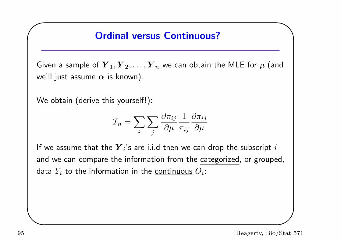
Multinomial Framework
Define:
• Yij = 1(Oi = j)
• Y i = vec(Yij)
• Hij = 1−∑j−1k=1 Yik Hi1 = 1
116 Heagerty, Bio/Stat 571
'
&
$
%
Multinomial Framework
Model:
E[Yij | Hij = 1] = µij
=πij
1− γi(j−1)
g(µij) = αj + Xijβj
j = 1, 2, . . . , C − 1
Note : E[Yij | Hij ] = µij ·Hij
117 Heagerty, Bio/Stat 571

'
&
$
%
Example:
j = 1, 2, . . . , 5
1 2 3 4 5
Yij 0 0 1 0 0
Hij 1 1 1 0 0
µij µi1 µi2 µi3 µi4 µi5
E[Yij | Hij ] µi1 µi2 µi3 0 0
118 Heagerty, Bio/Stat 571

'
&
$
%
Multinomial – CRM Models
• Models for E(Yij | Hij) are sometimes called “continuation ratio
models” (Agresti 1990).
• These conditional models are also known as discrete-time survival
models, in particular, if we assume that the ordered categories are time
intervals, Gj = (tj−1, tj ], and Oi records the interval that the time, Ti
falls in:
Oi = j ⇔ Ti ∈ Gj
119 Heagerty, Bio/Stat 571

'
&
$
%
Multinomial – CRM Models
PH Assumption : P (Ti > t) = exp[−Λ(t)]
= exp[−Λ0(t) exp(Xiβ)]
then
E(Yij | Hij = 1) = µij
log(− log(1− µij)) = αj + Xiβ
αj = log[Λ0(tj)− Λ0(tj−1)]
Note: The PH model uses a common β rather than a coefficient
specific to each time interval, βj .
120 Heagerty, Bio/Stat 571

'
&
$
%
CRM Model
• The multinomial probability factors:
P (Y i = yi) =C∏
j=1
πyij
ij
= P (yi1)P (yi2 | yi1)P (yi3 | yi1, yi2) . . .
. . . P (yiC | yik k < C)
121 Heagerty, Bio/Stat 571

'
&
$
%
CRM Model
P (Y i = yi) =C−1∏
j=1
(πij
1− γi(j−1)
)yij(
1− πij
1− γi(j−1)
)hij−yij
=C−1∏
j=1
(πij
1− γi(j−1)
)yij(
1− γij
1− γi(j−1)
)hij−yij
Note:
logit(πij
1− γi(j−1)) = log(
πij
1− γij)
122 Heagerty, Bio/Stat 571

'
&
$
%
Comments:
• This likelihood factorization implies that we obtain the MLE for this
model using the pairs (Yij , Hij = 1) and treating them as independent
Bernoulli random variables.
• For any (j, k)
E [(Yij − µijHij)(Yik − µikHik)] = 0
Q: justification for this?
123 Heagerty, Bio/Stat 571

WESDR Example:
#
nsubjects <- nrow( data )
#
wisc.data <- data.frame(
y = wisc.all.data[,"r.level"],
glyc.hemo = wisc.all.data[,"glyc.hemo"],
log.duration = log( wisc.all.data[,"duration"] ),
age.diag = wisc.all.data[,"age.diag"],
dia.bp = wisc.all.data[,"dia.bp"]
)
print( wisc.data[1:5,] )
#
###
### Construct CRM data...
###
#
##### (1) construct the pairs (Y,H)
#
123-1 Heagerty, Bio/Stat 571

ncuts <- max(wisc.data$y) - 1
print( paste("ncuts =", ncuts, "\n\n") )
y.crm <- NULL
h.crm <- NULL
id <- NULL
for( j in 1:nsubjects ){
yj <- rep( 0, ncuts )
if( wisc.data$y[j] <= ncuts ) yj[ wisc.data$y[j] ] <- 1
hj <- 1 - c(0,cumsum(yj)[1:(ncuts-1)])
y.crm <- c( y.crm, yj )
h.crm <- c( h.crm, hj )
id <- c( id, rep(j,ncuts) )
}
123-2 Heagerty, Bio/Stat 571

##### (2) construct the intercepts
#
level <- factor( rep(1:ncuts, nsubjects ) )
int.mat <- NULL
for( j in 1:ncuts ){
intj <- rep( 0, ncuts )
intj[ j ] <- 1
int.mat <- cbind( int.mat, rep( intj, nsubjects) )
}
dimnames(int.mat) <- list( NULL, paste("Int",c(1:ncuts),sep="") )
#
##### (3) expand the X’s
#
glyc.hemo <- rep( wisc.data$glyc.hemo , rep(ncuts,nsubjects) )
log.duration <- rep( wisc.data$log.duration , rep(ncuts,nsubjects) )
age.diag <- rep( wisc.data$age.diag , rep(ncuts,nsubjects) )
dia.bp <- rep( wisc.data$dia.bp , rep(ncuts,nsubjects) )
#
print( cbind( y.crm, h.crm, level, int.mat, glyc.hemo, log.duration,
age.diag, dia.bp)[1:15,] )
#
123-3 Heagerty, Bio/Stat 571

##### (4) drop the H=0 and build dataframe
#
keep <- h.crm==1
wisc.crm.data <- data.frame(
id = id[keep],
y = y.crm[keep],
level = level[keep],
glyc.hemo = glyc.hemo[keep],
log.duration = log.duration[keep],
age.diag = age.diag[keep],
dia.bp = dia.bp[keep] )
#
print( wisc.crm.data[1:15,] )
123-4 Heagerty, Bio/Stat 571

Original Data:
y glyc.hemo log.duration age.diag dia.bp
1 3 13.7 2.332144 29.9 89
2 2 13.5 2.292535 18.6 90
3 3 13.8 2.747271 28.7 85
4 1 8.4 3.540959 20.1 99
5 3 12.8 3.131137 29.3 84
123-5 Heagerty, Bio/Stat 571

Expanded Data:
id y.crm h.crm level Int1 Int2 Int3 glyc.hemo
[1,] 1 0 1 1 1 0 0 13.7
[2,] 1 0 1 2 0 1 0 13.7
[3,] 1 1 1 3 0 0 1 13.7
[4,] 2 0 1 1 1 0 0 13.5
[5,] 2 1 1 2 0 1 0 13.5
[6,] 2 0 0 3 0 0 1 13.5
[7,] 3 0 1 1 1 0 0 13.8
[8,] 3 0 1 2 0 1 0 13.8
[9,] 3 1 1 3 0 0 1 13.8
[10,] 4 1 1 1 1 0 0 8.4
[11,] 4 0 0 2 0 1 0 8.4
[12,] 4 0 0 3 0 0 1 8.4
[13,] 5 0 1 1 1 0 0 12.8
[14,] 5 0 1 2 0 1 0 12.8
[15,] 5 1 1 3 0 0 1 12.8
123-6 Heagerty, Bio/Stat 571

id y level glyc.hemo log.duration age.diag dia.bp
1 1 0 1 13.7 2.332144 29.9 89
2 1 0 2 13.7 2.332144 29.9 89
3 1 1 3 13.7 2.332144 29.9 89
4 2 0 1 13.5 2.292535 18.6 90
5 2 1 2 13.5 2.292535 18.6 90
6 3 0 1 13.8 2.747271 28.7 85
7 3 0 2 13.8 2.747271 28.7 85
8 3 1 3 13.8 2.747271 28.7 85
9 4 1 1 8.4 3.540959 20.1 99
10 5 0 1 12.8 3.131137 29.3 84
11 5 0 2 12.8 3.131137 29.3 84
12 5 1 3 12.8 3.131137 29.3 84
13 6 0 1 13.0 3.258097 21.8 70
14 6 0 2 13.0 3.258097 21.8 70
15 6 1 3 13.0 3.258097 21.8 70
123-7 Heagerty, Bio/Stat 571
'
&
$
%
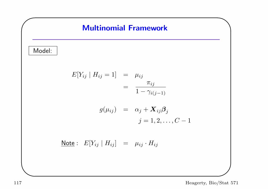
WESDR Models
#####
##### Model fitting...
#####
#
options( contasts="contr.treatment" )
#
table( wisc.crm.data$level )
#
fit1 <- glm( y ~ glyc.hemo, family=binomial,
subset=(as.integer(level)==1), data = wisc.crm.data )
summary( fit1, cor=F )
fit2 <- glm( y ~ glyc.hemo, family=binomial,
subset=(as.integer(level)==2), data = wisc.crm.data )
summary(fit2, cor=F )
fit3 <- glm( y ~ glyc.hemo, family=binomial,
124 Heagerty, Bio/Stat 571

'
&
$
%
subset=(as.integer(level)==3), data = wisc.crm.data )
summary(fit3, cor=F )
#
fit4 <- glm( y ~ level + glyc.hemo, family=binomial,
data = wisc.crm.data )
summary( fit4, cor=F )
fit5 <- glm( y ~ level * glyc.hemo, family=binomial,
data = wisc.crm.data )
#
anova( fit4, fit5 )
#
125 Heagerty, Bio/Stat 571

Separate fits:
table(level)
: 1 : 2 : 3
720 445 175
***LEVEL=1
Coefficients:
Value Std. Error t value
(Intercept) 0.22510208 0.38001813 0.5923456
glyc.hemo -0.05627671 0.02974703 -1.8918429
--------------------------------------------------
125-1 Heagerty, Bio/Stat 571

***LEVEL=2
Coefficients:
Value Std. Error t value
(Intercept) 1.01503739 0.48744691 2.082355
glyc.hemo -0.04551101 0.03731596 -1.219613
--------------------------------------------------
***LEVEL=3
Value Std. Error t value
(Intercept) 0.27807196 0.87839180 0.3165694
glyc.hemo 0.05636293 0.06755021 0.8343856
--------------------------------------------------
125-2 Heagerty, Bio/Stat 571

CRM fits:
Value Std. Error t value
(Intercept) 0.02245317 0.28434528 0.07896444
level: 2 0.92319834 0.12399549 7.44541891
level: 3 1.50031056 0.18751941 8.00082817
glyc.hemo -0.04008980 0.02184728 -1.83500205
(Dispersion Parameter for Binomial family taken to be 1 )
Null Deviance: 1857.608 on 1339 degrees of freedom
Residual Deviance: 1754.334 on 1336 degrees of freedom
Number of Fisher Scoring Iterations: 3
125-3 Heagerty, Bio/Stat 571

CRM fits:
Analysis of Deviance Table
Response: y
Terms Resid. Df Resid. Dev Test Df Deviance
1 level + glyc.hemo 1336 1754.334
2 level * glyc.hemo 1334 1751.906 +level:glyc.hemo 2 2.428885
125-4 Heagerty, Bio/Stat 571

'
&
$
%
Summary
• Multinomial models use a multivariate response vector to represent
the outcome.
• For these models the mean (πi) determines the covariance.
• Proportional odds models consider all possible dichotomizations.
• Continuation ratio models consider an ordered sequence of
conditional expectations.
126 Heagerty, Bio/Stat 571

'
&
$
%
References :
McCullagh & Nelder, Chapter 5 Polytomous Regression
Ananth C.V. and Kleinbaum D.G. (1997), “Regression models for
ordinal responses: A review of methods and applications”, Int J ofEpi, 26: 1323-1333.
Fahrmeir & Tutz, Chapter 3 Multicategorical responses
Agresti A. (1999), “Modelling ordered categorical data: recent
advances and future challenges”, Statistics in Medicine, 18:
2191-2207.
127 Heagerty, Bio/Stat 571