Multimodal Analysis Methodology of Urban Road Transport...

Document title Multimodal Analysis Methodology of Urban Road Transport Network Performance Deliverable D1.1

Authors Frederic Rudolph (Wuppertal Institut), Nora Szabo (PTV AG) Contributors Tamás Mátrai (Budapest University of Technology and Economics), Bernard

Gyergyay and Bonnie Fenton (Rupprecht Consult), Martin Wedderburn (Walk21), Andrew Nash

Status F Reviewed by Mark Crabtree and Dr Alan Stevens (TRL)

Submission date 27.07.2016

Multimodal Analysis Methodology of Urban Road

Transport Network Performance

A Base for Analysing Congestion Effects of Walking and Cycling Measures

www.h2020-flow.eu

FLOW I Multimodal Analysis Methodology of Urban Road Transport Network Performance 1

Release information Released by: FLOW project consortium

Document version: Final

Dissemination level: Public

Date of submission: 27 July 2016

Disclaimer The purpose of this document is to stimulate a European debate among mobility stakeholders. While it reflects the views of the authors, it does not comply with common practice and official definitions in all EU Member States.

The sole responsibility for the content of this publication lies with the authors. It does not necessarily reflect the opinion of the European Union. Neither the INEA nor the European Commission is responsible for any use that may be made of the information contained herein.

www.h2020-flow.eu

2 FLOW I Multimodal Analysis Methodology of Urban Road Transport Network Performance

TABLE OF CONTENTS

1. Introduction ............................................................................................................................................ 5

2. Definition of multimodal transport network performance and congestion .............................................. 7

3. Key Performance Indicators to describe the multimodal performance of an urban road transport network .................................................................................................................................................. 9

3.1. Determination of assessment level ...................................................................................................... 10

3.2. Priority setting amongst transport modes ............................................................................................ 11

3.3. Calculation of multimodal KPIs ............................................................................................................ 11

3.3.1. Delay ................................................................................................................................................... 13

3.3.2. Density ................................................................................................................................................. 16

3.3.3. Level of service .................................................................................................................................... 19

3.4. Aggregation of mode-specific KPIs into a multimodal performance index (MPI) ................................. 22

4. Determination of multimodal congestion threshold .............................................................................. 24

5. Demonstration through examples ........................................................................................................ 25

5.1. Example: Multimodal delay at a signalised junction ............................................................................ 25

5.2. Example: Multimodal delay along a corridor ........................................................................................ 28

5.3. Example: Multimodal density on road segment ................................................................................... 29

5.4. Example: Multimodal LOS at a signalised junction .............................................................................. 30

5.5. Example: Multimodal LOS on a road segment .................................................................................... 33

6. Achievements, limitations and outlook ................................................................................................ 34

6.1. Achievements ...................................................................................................................................... 34

6.2. Limitations ........................................................................................................................................... 34

6.2.1. Applicability on shared elements of the urban road transport network ................................................ 35

6.2.2. Understanding of perception of delay for users of different transport modes ...................................... 35

6.2.3. Moving people, not vehicles ................................................................................................................ 35

6.2.4. Understanding of network-wide multimodal LOS ................................................................................ 36

6.3. Outlook ................................................................................................................................................ 36

7. References .......................................................................................................................................... 37

www.h2020-flow.eu


LIST OF TABLES Table 1: Application of FLOW KPIs on network elements ............................................................................... 10 Table 2: An example of weighting factors set based on a hypothetical prioritisation of cycling ...................... 11 Table 3: LOS classes and thresholds for four modes at a signalised junction ................................................ 20 Table 4: LOS classes and thresholds for four modes on a road segment based ............................................ 21 Table 5: Transformation of LOS classes into utility points .............................................................................. 22 Table 6: Different aggregation possibilities offered by FLOW ......................................................................... 23 Table 7: Multimodal delay at a signalised junction before measure implementation ....................................... 26 Table 8: Multimodal delay at a signalised junction after measure implementation ......................................... 27 Table 9: Multimodal delay along a corridor before measure implementation .................................................. 28 Table 10: Multimodal delay along a corridor after measure implementation ................................................... 28 Table 11: Multimodal density on a road segment before measure implementation ........................................ 29 Table 12: Multimodal density on a road segment after measure implementation ........................................... 29 Table 13: Multimodal LOS at a junction before measure implementation ....................................................... 31 Table 14: Multimodal LOS at a junction after measure implementation .......................................................... 32 Table 15: Multimodal LOS on a road segment before measure implementation ............................................ 33 Table 16: Multimodal LOS on a road segment after measure implementation ............................................... 33

LIST OF FIGURES Figure 1: Common assumptions of cities .......................................................................................................... 5 Figure 2: Developmental steps of the FLOW Multimodal Transport Performance Analysis Methodology ....... 6 Figure 3: Four steps of calculation in the FLOW methodology ........................................................................ 10 Figure 4: Illustrative cross section with transport modes assessed ................................................................ 12 Figure 5: Example of mode-specific LOS at junctions along a route ............................................................... 21 Figure 6: Measure overview: multimodal delay at a signalised junction ......................................................... 25 Figure 7: Measure overview: multimodal delay along a corridor ..................................................................... 28 Figure 8: Measure overview: multimodal density on road segment ................................................................ 29 Figure 9: Measure overview: multimodal LOS at a signalised junction ........................................................... 30 Figure 10: Measure overview: multimodal LOS on a road segment ................................................................ 33

www.h2020-flow.eu

4 FLOW I Multimodal Analysis Methodology of Urban Road Transport Network Performance

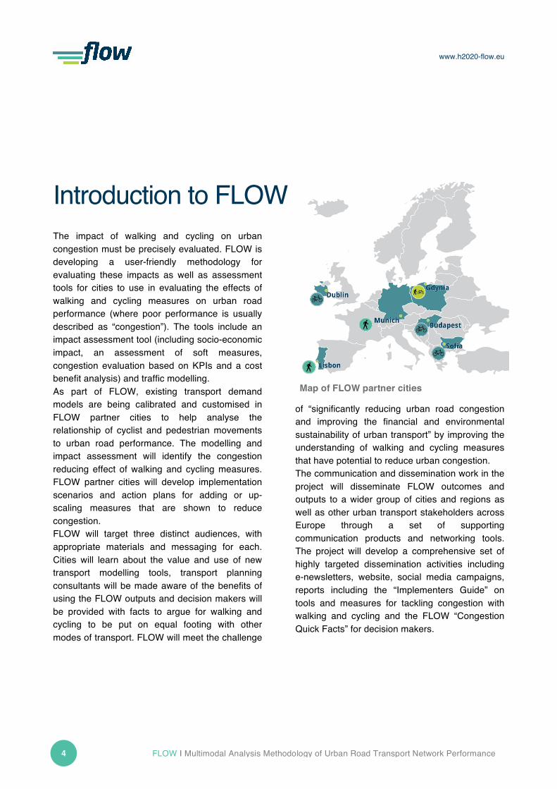
Introduction to FLOW The impact of walking and cycling on urban congestion must be precisely evaluated. FLOW is developing a user-friendly methodology for evaluating these impacts as well as assessment tools for cities to use in evaluating the effects of walking and cycling measures on urban road performance (where poor performance is usually described as “congestion”). The tools include an impact assessment tool (including socio-economic impact, an assessment of soft measures, congestion evaluation based on KPIs and a cost benefit analysis) and traffic modelling. As part of FLOW, existing transport demand models are being calibrated and customised in FLOW partner cities to help analyse the relationship of cyclist and pedestrian movements to urban road performance. The modelling and impact assessment will identify the congestion reducing effect of walking and cycling measures. FLOW partner cities will develop implementation scenarios and action plans for adding or up-scaling measures that are shown to reduce congestion. FLOW will target three distinct audiences, with appropriate materials and messaging for each. Cities will learn about the value and use of new transport modelling tools, transport planning consultants will be made aware of the benefits of using the FLOW outputs and decision makers will be provided with facts to argue for walking and cycling to be put on equal footing with other modes of transport. FLOW will meet the challenge

of “significantly reducing urban road congestion and improving the financial and environmental sustainability of urban transport” by improving the understanding of walking and cycling measures that have potential to reduce urban congestion. The communication and dissemination work in the project will disseminate FLOW outcomes and outputs to a wider group of cities and regions as well as other urban transport stakeholders across Europe through a set of supporting communication products and networking tools. The project will develop a comprehensive set of highly targeted dissemination activities including e-newsletters, website, social media campaigns, reports including the “Implementers Guide” on tools and measures for tackling congestion with walking and cycling and the FLOW “Congestion Quick Facts” for decision makers.

Map of FLOW partner cities

www.h2020-flow.eu


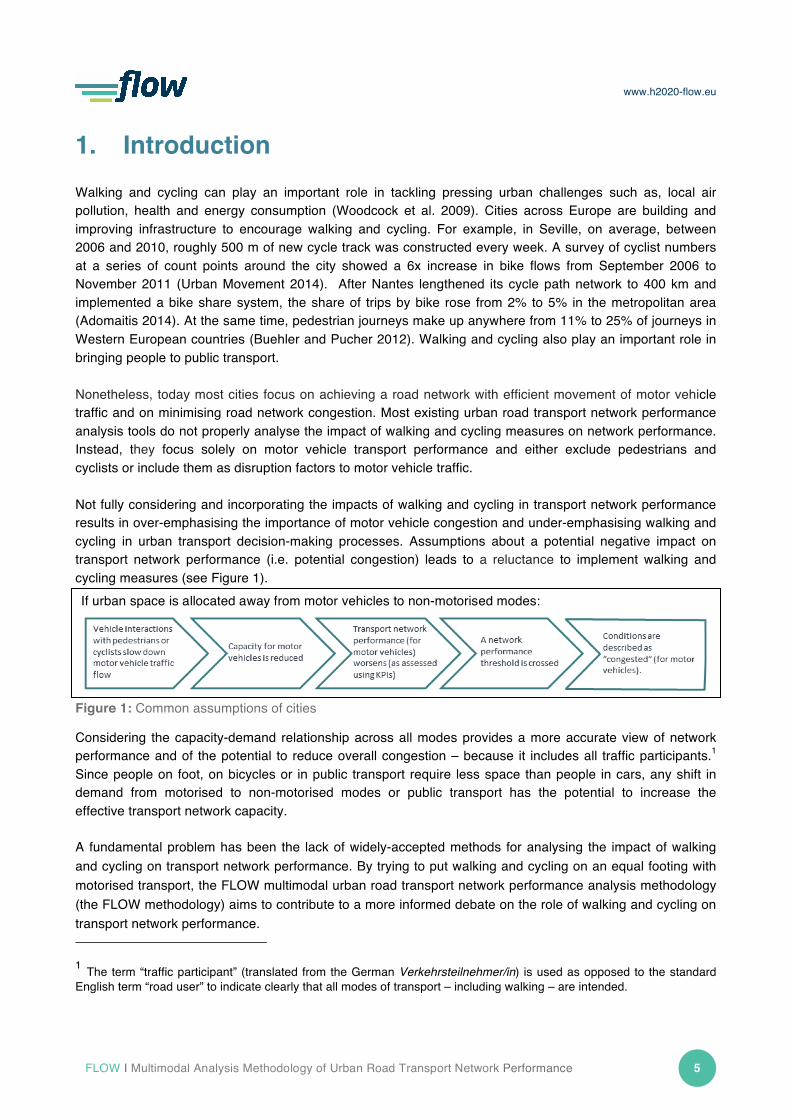
1. Introduction Walking and cycling can play an important role in tackling pressing urban challenges such as, local air pollution, health and energy consumption (Woodcock et al. 2009). Cities across Europe are building and improving infrastructure to encourage walking and cycling. For example, in Seville, on average, between 2006 and 2010, roughly 500 m of new cycle track was constructed every week. A survey of cyclist numbers at a series of count points around the city showed a 6x increase in bike flows from September 2006 to November 2011 (Urban Movement 2014). After Nantes lengthened its cycle path network to 400 km and implemented a bike share system, the share of trips by bike rose from 2% to 5% in the metropolitan area (Adomaitis 2014). At the same time, pedestrian journeys make up anywhere from 11% to 25% of journeys in Western European countries (Buehler and Pucher 2012). Walking and cycling also play an important role in bringing people to public transport. Nonetheless, today most cities focus on achieving a road network with efficient movement of motor vehicle traffic and on minimising road network congestion. Most existing urban road transport network performance analysis tools do not properly analyse the impact of walking and cycling measures on network performance. Instead, they focus solely on motor vehicle transport performance and either exclude pedestrians and cyclists or include them as disruption factors to motor vehicle traffic. Not fully considering and incorporating the impacts of walking and cycling in transport network performance results in over-emphasising the importance of motor vehicle congestion and under-emphasising walking and cycling in urban transport decision-making processes. Assumptions about a potential negative impact on transport network performance (i.e. potential congestion) leads to a reluctance to implement walking and cycling measures (see Figure 1).

Figure 1: Common assumptions of cities

Considering the capacity-demand relationship across all modes provides a more accurate view of network performance and of the potential to reduce overall congestion – because it includes all traffic participants.1 Since people on foot, on bicycles or in public transport require less space than people in cars, any shift in demand from motorised to non-motorised modes or public transport has the potential to increase the effective transport network capacity. A fundamental problem has been the lack of widely-accepted methods for analysing the impact of walking and cycling on transport network performance. By trying to put walking and cycling on an equal footing with motorised transport, the FLOW multimodal urban road transport network performance analysis methodology (the FLOW methodology) aims to contribute to a more informed debate on the role of walking and cycling on transport network performance. 1 The term “traffic participant” (translated from the German Verkehrsteilnehmer/in) is used as opposed to the standard English term “road user” to indicate clearly that all modes of transport – including walking – are intended.

If urban space is allocated away from motor vehicles to non-motorised modes:

www.h2020-flow.eu

6 FLOW I D1.1 Multimodal Analysis Methodology of Urban Road Transport Network Performance

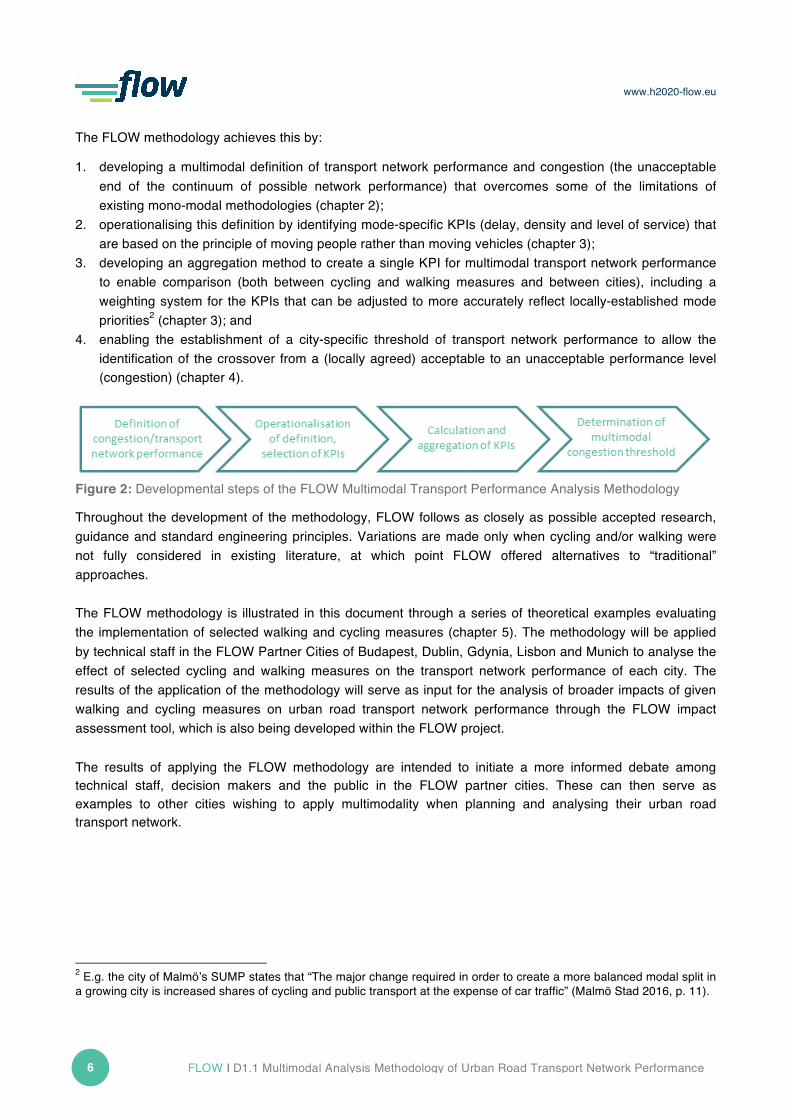
The FLOW methodology achieves this by:

1. developing a multimodal definition of transport network performance and congestion (the unacceptable end of the continuum of possible network performance) that overcomes some of the limitations of existing mono-modal methodologies (chapter 2);

2. operationalising this definition by identifying mode-specific KPIs (delay, density and level of service) that are based on the principle of moving people rather than moving vehicles (chapter 3);

3. developing an aggregation method to create a single KPI for multimodal transport network performance to enable comparison (both between cycling and walking measures and between cities), including a weighting system for the KPIs that can be adjusted to more accurately reflect locally-established mode priorities2 (chapter 3); and

4. enabling the establishment of a city-specific threshold of transport network performance to allow the identification of the crossover from a (locally agreed) acceptable to an unacceptable performance level (congestion) (chapter 4).

Figure 2: Developmental steps of the FLOW Multimodal Transport Performance Analysis Methodology

Throughout the development of the methodology, FLOW follows as closely as possible accepted research, guidance and standard engineering principles. Variations are made only when cycling and/or walking were not fully considered in existing literature, at which point FLOW offered alternatives to “traditional” approaches. The FLOW methodology is illustrated in this document through a series of theoretical examples evaluating the implementation of selected walking and cycling measures (chapter 5). The methodology will be applied by technical staff in the FLOW Partner Cities of Budapest, Dublin, Gdynia, Lisbon and Munich to analyse the effect of selected cycling and walking measures on the transport network performance of each city. The results of the application of the methodology will serve as input for the analysis of broader impacts of given walking and cycling measures on urban road transport network performance through the FLOW impact assessment tool, which is also being developed within the FLOW project. The results of applying the FLOW methodology are intended to initiate a more informed debate among technical staff, decision makers and the public in the FLOW partner cities. These can then serve as examples to other cities wishing to apply multimodality when planning and analysing their urban road transport network.

2 E.g. the city of Malmö’s SUMP states that “The major change required in order to create a more balanced modal split in a growing city is increased shares of cycling and public transport at the expense of car traffic” (Malmö Stad 2016, p. 11).

www.h2020-flow.eu


2. Definition of multimodal transport network performance and congestion

The FLOW project began with an extensive examination of the literature on transport network performance. While the examination included all types of performance measures, it focused on congestion since that is the performance measure most closely linked to transport system quality by technical staff, decision-makers and the public. In examining existing definitions of congestion (e.g., Weisbrod et al. 2001, Bovy and Salomon 2002, Stopher 2004, Litman 2015), the FLOW project found that most definitions focus solely on motorised road transport, effectively ignoring a significant portion of urban transport. There is currently no generally accepted multimodal definition of transport network performance or congestion. It also became clear that congestion lies at one end of a spectrum of transport network performance, where the other end is free flowing traffic. But the point where “non-congested” becomes “congested” is not easily defined, and indeed varies from city to city and is perceived differently from traffic participant to traffic participant. In an effort to address the identified shortcomings of earlier definitions, the FLOW project defines congestion as follows:3

Congestion is a state of traffic involving all modes on a multimodal transport network (e.g. road, cycle facilities, pavements, bus lane) characterised by high densities and overused infrastructure compared to an acceptable state across all modes against previously-agreed targets and thereby leads to (perceived or actual) delay.

This definition:

1. includes urban transport infrastructure for all modes (both motorised and non-motorised); 2. refers to both demand and capacity; 3. leaves sufficient flexibility to adapt to local circumstances; and 4. accounts for user perceptions.

Both motorised and non-motorised modes “…involving all modes on an integrated transport network (e.g. road, cycle facilities, pavements, bus lane)…”

Considering the capacity-demand relationship across all modes provides a more accurate view of network performance and of the potential to reduce overall congestion (because it includes all traffic participants). Since people on foot, on bicycles or in public transport require less space than people in cars, any shift in demand from motorised to non-motorised or public transport modes has the potential to increase the effective transport network capacity.

Demand and capacity “…characterised by high densities and overused infrastructure...”

The consideration of demand and capacity is a fundamental element of traffic engineering and is therefore 3 The definition was developed in an iterative process of literature review, expert consultation and internal discussion.

www.h2020-flow.eu


also part of the FLOW definition. The important distinction between traditional definitions of congestion and the FLOW definition is that FLOW considers demand and capacity for all modes of transport and takes into account the fact that demand on infrastructure capacity varies significantly between transport modes. It also allows for the fact that perceptions of the threshold at which infrastructure is “overused” may depend on the specific context and on the characteristics of the traffic participants.

Adaptability to local circumstances “…compared to an acceptable state across all modes against previously-agreed targets…”

Providing adaptability to local circumstances reflects the fact that cities have different transport characteristics and policy goals and that congestion reduction is only one objective. Thus the threshold for an “acceptable state” can vary from city to city (influenced, for example, by policies developed in a sustainable urban mobility – or similar – plan). “Previously-agreed targets” (i.e. a city’s established goals) can be incorporated using a weighting system to reflect the local context, goals and needs.

The user perspective …leads to (perceived or actual) delay….”

The user perspective is an important part of a multimodal definition. Delay is perceived by most traffic participants as a main impact of congestion (UK DfT 2001). User perceptions of different transport modes determine mobility behaviour and congestion is just one of a number of factors of interest to travellers (Pooley et al. 2013). FLOW recognises that travel times are relative. Delay is experienced by a traffic participant if the actual travel time exceeds a threshold that is perceived as acceptable. Further, perception of delay is not linear with increase in delay. It is also a function of journey purpose, of the proportion of the delay of the overall journey time and other specific additional constraints such as a need to meet a public transport connection. As an example, empirical evidence in Sweden shows that cyclists value their travel time differently depending on the attractiveness and safety of the transport network. The safer and more comfortable the transport infrastructure elements are perceived to be, the lower the perception of the value of travel time saved. Accordingly, ‘acceptable’ travel time may increase with cycling infrastructure that is perceived as better (Börjesson and Eliasson, 2012). Because there is a lack of research on “acceptable” delay for walking and cycling, FLOW has adopted minimum travel time as a reference value to operationalise acceptable travel time for all modes and suggests default values for minimum travel time for car drivers, cyclists and pedestrians (chapter 3.3.1), thereby contributing to a multimodal understanding of traffic flow and congestion.4

4 Minimum travel time from the user’s perspective should not be confused with travel time reliability. The FLOW methodology deals with urban road transport network performance. Under urban conditions, congestion is recurrent and predictable and thus reliable.

www.h2020-flow.eu


3. Key Performance Indicators to describe the multimodal performance of an urban road transport network

Chapter three presents the key performance indicators (KPIs) developed in the FLOW project. The primary aim of the KPIs is to operationalise the project’s multimodal definition of transport network performance and congestion in terms of the demand-supply relationship and of travel-time related aspects. The selected indicators describe the state of traffic flow, enabling the analysis of transport network performance for all modes using objective measures. While the indicators aim to relate to user perceptions of transport network performance, the operationalised KPIs cannot fully reflect the spatial, temporal and personal variations in user perception understood in the FLOW definition of multimodal transport network performance due to the lack of an empirical base, particularly for the KPI ‘delay’. The selection, calculation and refinement of KPIs was based on a literature review and expert input. The selected KPIs were the most applicable in a multimodal context and for the assessment levels used in FLOW (see chapter 3.1). The FLOW project selected the following three key performance indicators (based on FGSV 2015):

1. Delay is the additional travel time experienced by a traffic participant as compared to the minimum travel time.

2. Density is a measure of the number of persons or vehicles using a given space.5 3. Level of service (LOS) is an indicator that seeks to reflect the quality of service experienced by

traffic participants under different levels of use of infrastructure.

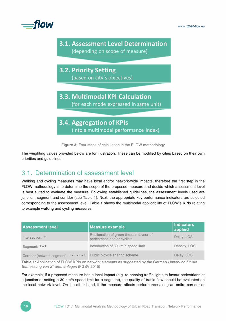
These indicators can be used for local or network level analysis, and can be calculated for each transport mode separately. The KPIs are described in more detail in Chapter 3.3. An important innovative aspect of the FLOW methodology is also using the unit “person” for all modes for the KPI ‘delay’ following the principle “moving people, not vehicles”. This provides a common numerical basis for comparing the efficiency of different transport modes. (Because traffic engineering principles do not allow the same translation for density, these mode-specific values are handled separately). In an additional step different mode-specific KPI values are aggregated into a single multimodal KPI – called MPI – by calculating a weighted average. The methodology for calculating the KPIs consists of four steps, as illustrated in Figure 3. Each step is explained separately in the following sections, including a definition and computation procedures.

5 Density: persons per m2 for pedestrians, vehicles per lane per km for motor vehicles and bicycles.

www.h2020-flow.eu


Figure 3: Four steps of calculation in the FLOW methodology

The weighting values provided below are for illustration. These can be modified by cities based on their own priorities and guidelines.

3.1. Determination of assessment level Walking and cycling measures may have local and/or network-wide impacts, therefore the first step in the FLOW methodology is to determine the scope of the proposed measure and decide which assessment level is best suited to evaluate the measure. Following established guidelines, the assessment levels used are junction, segment and corridor (see Table 1). Next, the appropriate key performance indicators are selected corresponding to the assessment level. Table 1 shows the multimodal applicability of FLOW’s KPIs relating to example walking and cycling measures.

Assessment level Measure example Indicators applied

Intersection: + Reallocation of green times in favour of pedestrians and/or cyclists Delay, LOS

Segment: +-+ Introduction of 30 km/h speed limit Density, LOS

Corridor (network segment): +-+-+-+ Public bicycle sharing scheme Delay, LOS

Table 1: Application of FLOW KPIs on network elements as suggested by the German Handbuch für die Bemessung von Straßenanlagen (FGSV 2015)

For example, if a proposed measure has a local impact (e.g. re-phasing traffic lights to favour pedestrians at a junction or setting a 30 km/h speed limit for a segment), the quality of traffic flow should be evaluated on the local network level. On the other hand, if the measure affects performance along an entire corridor or

www.h2020-flow.eu


network segment (e.g., building a cycle track along a corridor or implementing a public bike-sharing scheme), network-wide performance should be evaluated. In most cases, it is valuable to assess both local and network level impacts.

3.2. Priority setting amongst transport modes FLOW’s evaluation of transport network performance (and thus congestion) consists of taking single, mode-specific KPI values and aggregating them into an average. However, FLOW recognises that each city establishes its own priorities. Many have sustainable urban mobility planning processes that facilitate decision making. One outcome of such a process may be a decision to prioritise walking, cycling and public transport over car travel. FLOW facilitates this prioritisation by including a weighting factor. Using the methodology, a city may set a weighting factor for each transport mode with reference to the city’s established priorities. This weighting factor recognises that cities may have transport policies emphasising the various positive impacts of walking and cycling (e.g. promotion and financial support for non-motorised modes) based on their strategic objectives. These priorities can be set for the entire network or for parts of it. For example, a cycle highway will have a higher priority for cycling than a pedestrian area. The default value for this weighting is set to 1 (i.e., all transport modes have the same weighting) to ensure comparability of the effect of a single measure across different cities. Table 2 presents an example of mode-specific weighting factors.

Table 2: An example of weighting factors set based on a hypothetical prioritisation of cycling

3.3. Calculation of multimodal KPIs The FLOW methodology calculates multimodal (rather than the traditional mono-modal) key performance indicators for an urban road transport network. This section defines, describes and explains the relevance of the KPIs and provides an illustrative calculation. The formulas and calculation procedure are provided for the FLOW KPIs (delay, density and LOS) – with variation depending on the scope and impact of a proposed measure. These KPIs are calculated separately for cars, public transport vehicles, cyclists and pedestrians, as depicted in the example cross section (Figure 4). In the fourth step, these individual KPIs (except for density, see p. 10) are aggregated to create a single multimodal KPI.

Measure Affected network element Transport mode

Weighting factor

car 1public transport 1

cyclist 3pedestrian 1

prioritisation of cycling: construction of a new cycling lane

separate cycle lane (extension)lanes for motorised traffic (reduced width)

www.h2020-flow.eu


Figure 4: Illustrative cross section with transport modes assessed

The basic input data are computed with the help of transport simulation models. The scale of the measure suggests whether microscopic or macroscopic transport models should be used for the analysis, specifically:

• Local congestion analysis: microscopic simulation • Corridor or network level congestion analysis: depending on the measure, either macroscopic or

microscopic models or both can be used. However, considering pedestrians in macroscopic models may be difficult as most pedestrian trips are intra-zonal due to cell sizes that are larger than the average length of a pedestrian trip).

Given the need for model data, a prerequisite for calculating the FLOW congestion KPIs is a well-calibrated multimodal model in terms of transport demand and supply for private vehicles, public transport, bicycles and pedestrians. FLOW addresses recurring urban congestion (as opposed to congestion caused by unpredicted events). This mainly occurs in peak periods (e.g. weekday morning or evening peaks or shopping traffic at the weekend). Thus the KPIs are calculated for the period with the highest hourly traffic volumes. In addition to travel demand, geometry (e.g. number of lanes, advance stop boxes, width of sidewalk and cycle lane), parameters for realistic travel behaviour (e.g. pedestrians and cyclists of different age groups), service characteristics for public transport and junction control (e.g. traffic signal timing) are also needed for the computation. If a multimodal transport model is not available, numerical calculation procedures may also be used to calculate the KPIs. In this case, decisive variables – relying on the input data obtained from multimodal traffic counts or surveys – are calculated by means of formulas and empirical curves provided in national or international guidelines such as the US Highway Capacity Manual (TRB 20106) and the German Highway Capacity Manual (Handbuch für Bemessung von Straßenverkehrsanlagen, FGSV 2015). As noted above, an important aspect of the FLOW method for calculating the selected KPIs is that the variables are expressed in persons rather than vehicles. This provides a basis for comparing the efficiency of different transport modes. Therefore, the FLOW methodology calculates an average delay per person for each transport mode either on the local (junction or segment) or network (corridor) level. The transformation of vehicle-based values into person-based values can only be applied to delay calculations. Mode-specific density values are expressed in their original units (veh/km for cars and bicycles, ped/m2 or ped/km for one-dimensional pedestrian movement) following traffic engineering principles, since transforming these density data into per person values would lead to an inevitable loss of significance of the single values. For the same reason, they are also not aggregated to a multimodal performance index in later stages (see chapter 3.4).

6 An update will be released in summer 2016.

www.h2020-flow.eu


In the KPI ‘level of service’, FLOW assigns calculated, mode-specific vehicle-based delay and density values (or other basic indicators as recommended by TRB 2010 or FGSV 2015, described in chapter 3.3) to LOS classes. These values are designed to give the same consideration to each mode. This concept attempts to overcome the current bias in LOS classification, wherein thresholds for motorised traffic are used as the decisive variables for evaluating performance at a junction, and delays for non-motorised transport are used solely as a recommendation for consideration in a quality check.

3.3.1. Delay

Definition Delay is commonly defined as the mean time loss per traffic participant along a route – with the general assumption being motorised transport. It is calculated as the difference between the actual travel time and the minimum travel time (free-flow conditions). For car drivers, FLOW applies this generally accepted definition of minimum travel time being free-flow conditions as it is an established benchmark in traffic engineering practice. For cyclists, minimum travel time is defined as the average cycling speed (cycling speeds can vary greatly but an average cycling speed of 15 kilometres per hour is commonly assumed) multiplied by the distance over the network from origin to destination. In this case the network can include roadways without cycling facilities. For pedestrians, minimum travel time is defined as the time it would take to walk as the crow flies between two defined points at an average walking speed (walking speeds vary greatly depending on users, geography and culture, but average speeds of between 1.2 and 1.4 metres per second are commonly used in Europe). This definition recognises the nature of pedestrian movement and can be applied to the dispersed movements encountered at major junctions and in public spaces as well movement along defined links. The difference between the established minimum travel time and actual travel time (delay) can have different magnitudes for different modes. A pre-requisite for the calculation of delay is that it is consistent over all scenarios and transport modes, representing the same value on the same route. For example, a before-after comparison should always account for the initial delay due to the presence of traffic control devices. However, as noted in chapter 2, not enough is known about the perception of delay for various modes of transport. Further research on acceptable (as opposed to minimum) travel time from a multimodal perspective could replace the easily calculated – but oversimplified – proxy of minimum travel time. In the urban context, additional travel time is often caused by traffic delays from control devices (e.g., traffic signals) (TRB 2010). As established in technical guidelines, control delay is calculated at signalised and unsignalised junctions, including delay associated with cars, buses, bicycles and also pedestrians – and their interactions.

Calculation The FLOW project recommends two different network level-related calculation procedures depending on the scope of a walking or cycling measure. These procedures use input variables from multimodal transport simulation models or formulas from national or international guidelines. The KPIs are calculated for each transport mode separately.

www.h2020-flow.eu


Example: Calculation of local level delay at a junction Delay is calculated at the local level for a junction. Control delay is a direct output variable of the microscopic multimodal transport simulation, hence no additional calculation procedure is needed at this level. Delay values are computed for each lane or turning movement7, for all means of transport and all junction control types. The delay “td,k,i” is a function of the variables listed below:

𝑡!,!,!

Where

td,k,i = decisive mean delay td on turning movement i on each approach of the junction, or at junction crossing for transport mode k [s/veh or s/ped]

Delay for public transport vehicles at stop lines of a junction depends on the signal programme (whether priority is given to public transport vehicles) and results from the given timetable. Alternately, if transport models are not available, mode-specific numerical calculation procedures are provided for every junction control type, separately for all transport modes.8,9

Example: Calculation of network level delay along a corridor The simplified calculation procedure measuring delay along an entire route (start point to end points) corresponds to the difference between the actual and minimum travel time (see justification for the use of minimum travel time in chapter 2):

𝑡!,! = 𝑡!"#,! − 𝑡!,!

Where

td,k = total delay td along the route for transport mode k [s/veh or s/pers]

tact,k = actual travel time along the route for transport mode k [s/veh or s/pers]

t0,k = minimum travel time along the route for transport mode k [s/veh or s/pers]

7 Turning movements at junctions are defined as left turn, right turn or straight ahead movement. 8 TRB 2010, chapters 18-21 for single (signalised and unsignalised) junctions. 9 FGSV 2015, chapters 4-5 for single (signalised and unsignalised) junctions.

www.h2020-flow.eu


Both the mode-specific actual travel time and the minimum travel time are direct outputs of the transport model. The actual travel time is computed using the following formula:

𝑡!"#,! = 𝑠! ∙ 3,6𝑣!"#,!

Where

tact,k = actual travel time along the route for transport mode k [s/veh or s/pers]

sk = distance travelled along the route for transport mode k [m/veh] or length of trajectory walked for pedestrians [m/pers]

vact,k = actual speed along the route for transport mode k [km/h]

The minimum travel time is computed using the following formula:

𝑡!,! = 𝑠! ∙ 3,6𝑣!,!

Where

t0,k = minimum travel time in free flow conditions along the route for transport mode k [s/veh or s/pers]

sk = distance travelled along the route for transport mode k [m/veh] or crow fly distance from origin to destination for pedestrians [m/pers]

v0,k = maximum permissible or desired speed along the route for transport mode k [km/h]

Additional care is needed when calculating pedestrian delay due to pedestrians’ unrestricted movement in the network. Here, the calculation of actual travel time can be computed more realistically by fully considering detours taken to avoid obstacles, level differences, lack of access to prohibited areas and the indirectness of crossings. These types of measurements can be partially derived from existing microscopic models but in practice they are generally calculated manually based on walking distance, an average walking speed and observed or modelled delays on individual arms of junctions (see above). At the network level it is also possible to calculate delay without using a transport model as a source of basic input variables. In this case, the total delay along the route is calculated by means of formulas provided by international or national highway capacity manuals.10 The control delays at junctions and other delays occurring in the vicinity of junctions can be summed. For a precise delay calculation, the control type at each junction along the route must be known because the calculation of single delay values occurs separately for each control type.

10 Chapter 16 in the Highway Capacity Manual (TRB 2010) for delay calculation on urban street facilities and chapter six in the German Highway Capacity Manual (FGSV 2015).

www.h2020-flow.eu


Example: Calculation of person-related delays A fundamental part of the FLOW methodology is considering person-related (as opposed to vehicle-related) delays to provide a common basis for comparison amongst different means of transport. Therefore the mean delay per lane per vehicle on both network levels needs to be scaled by the number of persons. In this case, the lane-based delay per person is equal to the lane-based delay per vehicle. Here, the mean delay per transport entity (not the total delay over the whole network) is considered and therefore it is not necessary to multiply the delay results by vehicle occupancy ratio.

3.3.2. Density Vehicle density is a recommended indicator for determining transport network performance and assessing roadway segment congestion in most technical guidelines because high densities often lead to traffic delays.

Definition FLOW adopts the commonly accepted definition of density (TRB 2010, FGSV 2015). This definition is based on the proximity of vehicles or persons to one another. Density is defined as the number of vehicles (cars, public transport vehicles or bicycles) as well as persons, occupying a given length of roadway lane, usually specified as one kilometre.

Example: calculation of road segment density at the local level Density on a road segment between two adjacent junctions (outside of the junction areas) is calculated for each lane individually following similar calculation principles for all modes except pedestrians. The basic input variables for the density computation are outputs of the multimodal transport model.11 If no transport model is available, the input variables may be gathered from traffic counts and on-site speed measurements in the peak hour. Single density values are calculated for each lane separately using the recommended units of veh/km for vehicles and pers/m2 for pedestrians assuming that each lane is used by a single means of transport. An alternative for calculating on shared facilities can be found at the end of this section. A transformation of pedestrian area-based density into lane-based density is needed to provide the same units for comparison. A precondition is a pedestrian area wherein pedestrians move single-file bi-directionally – typically on a sidewalk next to road.

11 On the microscopic level, density may also be taken as a direct output variable of the transport simulation.

www.h2020-flow.eu


Vehicles: cars and bicycles The most widely used formula for calculating vehicle density makes use of the three variables of the fundamental diagram12. Density on a lane for vehicles (separate mode calculation for cars and cyclists) is computed based on the following basic equation (FGSV 2015):

𝐷! =𝑞!𝑣!

Where

Di = density for transport mode i [veh/km]

qi = decisive traffic volume per lane for transport mode i in the peak hour [veh/h] – output of transport model or result of traffic counts. If traffic flow is not given by lane but rather link-based per direction (on the macroscopic level), an additional adjustment factor for the distribution of traffic between lanes has to be employed, depending on the number and width of lanes. One possible adjustment factor is available in FGSV 2015, but as an approximation, link-based traffic flow can be divided by the number of lanes to assess lane-based flow.

vi = (space) average travel speed for transport mode i [km/h] – output of transport model calculated by the average distance the vehicles move on a road segment within a short time span, divided by that time span. Average speed can also be read from empirical q-V curves.13

For bicycle traffic, different cycling behaviour parameters are needed depending on the type of cycling facility (i.e. if it is wide enough for cyclists to overtake or if they must ride single-file in a bicycle lane).

Vehicles: public transport The FLOW methodology offers a simplified computation procedure for public transport vehicle density. More specifically, where public transport traffic uses a separate lane and therefore has its own density value. This approach is arguably meaningful in cities with heavy bus traffic (such as the FLOW cities of Dublin or Budapest), where high level of bus demand leads to traffic jams even in dedicated bus lanes. Similar to density calculation for cars, the following equation is applied to public transport density calculation:

𝐷 =𝑞𝑣

Where

D = density of public transport vehicles [veh/km]

q = traffic flow on a dedicated lane in the peak hour [veh/h]

v = average transit travel speed [km/h] – output of transport model or calculated based on the average transport time

12 The fundamental diagram (and fundamental equation) of traffic flow describes the relation between the traffic flux (in vehicles per hour) and traffic density (in vehicles per kilometre). For a more detailed explanation, see Lighthill and Whitham (1955). 13 One possible curve is given in chapter three of the German Highway Capacity Manual (FGSV 2015).

www.h2020-flow.eu


Pedestrians Pedestrian density is a direct output of a microscopic transport model, expressed in person/m2. These models use several different schemes to calculate pedestrian density.14 In order to provide a common basis for comparing pedestrian density with other transport modes, FLOW recommends that area-based density on a sidewalk along the road corridor (characterised by one-dimensional movement along an extended rectangle) needs to be normalised (person/km) using the following formula:

𝐷!"#,!! = 𝐷!"#,!! ∙ 𝑤 ∙ 1000

Where

Dped,1D = one-dimensional pedestrian density on a sidewalk next to a road corridor [persons/km]

Dped,2D = area-based pedestrian density on a sidewalk [persons/m2] – output of a transport model or the result of traffic counts

w = effective width of a sidewalk (depending on the presence of obstacles, street typology etc.) [m]

If pedestrian traffic is not simulated within a transport model, theoretical density may be calculated manually according to international or national guidelines. Shared facilities The calculation procedures offered by FLOW are based on a traffic lane being used by a single transport mode: car lanes by cars, bus lanes by buses, sidewalks by pedestrians and cycle lanes or paths by cyclists. However, traffic on road facilities shared by more than one transport mode should not be neglected. Road space can be shared by the following pairs of modes:

• Car and cycle • Public transport vehicle and car • Public transport vehicle and cycle • Pedestrian and cycle When lanes are shared certain assumptions have to be made to calculate transport system performance. One method is calculating lane-based density by transforming the hourly travel demand of each transport mode into passenger car units (PCU). Default values are 2 PCU for a bus and 0.5 PCU for a cyclist. An approximate speed for mixed traffic – for the density calculation – is then calculated. Pedestrian space may also be shared with cyclists. Where the shared facility consists of delineated space for each mode, lane-based use can be assumed. Where the shared path or space does not include specifically delineated cycle facilities, the FLOW calculation procedure for pedestrian density can be applied and amended to account for the presence of cyclists.

14 e.g. Fruin (1971), TRB (2010), FGSV (2015)

www.h2020-flow.eu


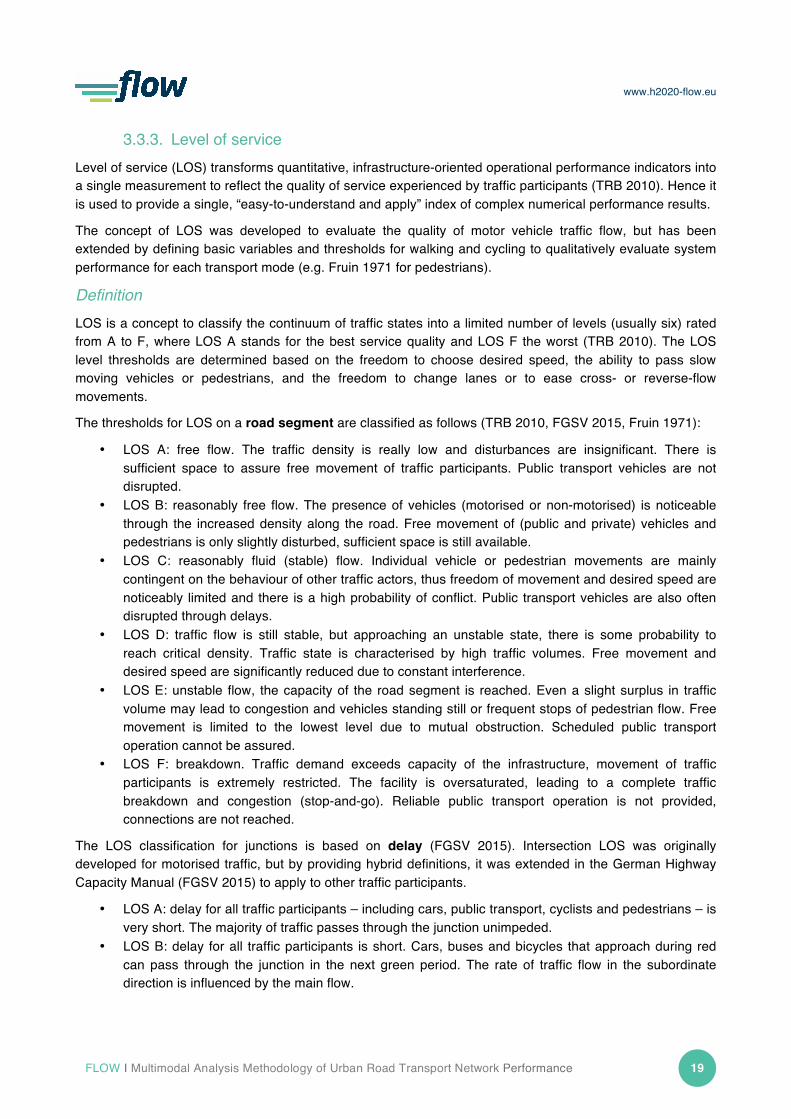
3.3.3. Level of service

Level of service (LOS) transforms quantitative, infrastructure-oriented operational performance indicators into a single measurement to reflect the quality of service experienced by traffic participants (TRB 2010). Hence it is used to provide a single, “easy-to-understand and apply” index of complex numerical performance results.

The concept of LOS was developed to evaluate the quality of motor vehicle traffic flow, but has been extended by defining basic variables and thresholds for walking and cycling to qualitatively evaluate system performance for each transport mode (e.g. Fruin 1971 for pedestrians). Definition LOS is a concept to classify the continuum of traffic states into a limited number of levels (usually six) rated from A to F, where LOS A stands for the best service quality and LOS F the worst (TRB 2010). The LOS level thresholds are determined based on the freedom to choose desired speed, the ability to pass slow moving vehicles or pedestrians, and the freedom to change lanes or to ease cross- or reverse-flow movements.

The thresholds for LOS on a road segment are classified as follows (TRB 2010, FGSV 2015, Fruin 1971):

• LOS A: free flow. The traffic density is really low and disturbances are insignificant. There is sufficient space to assure free movement of traffic participants. Public transport vehicles are not disrupted.

• LOS B: reasonably free flow. The presence of vehicles (motorised or non-motorised) is noticeable through the increased density along the road. Free movement of (public and private) vehicles and pedestrians is only slightly disturbed, sufficient space is still available.

• LOS C: reasonably fluid (stable) flow. Individual vehicle or pedestrian movements are mainly contingent on the behaviour of other traffic actors, thus freedom of movement and desired speed are noticeably limited and there is a high probability of conflict. Public transport vehicles are also often disrupted through delays.

• LOS D: traffic flow is still stable, but approaching an unstable state, there is some probability to reach critical density. Traffic state is characterised by high traffic volumes. Free movement and desired speed are significantly reduced due to constant interference.

• LOS E: unstable flow, the capacity of the road segment is reached. Even a slight surplus in traffic volume may lead to congestion and vehicles standing still or frequent stops of pedestrian flow. Free movement is limited to the lowest level due to mutual obstruction. Scheduled public transport operation cannot be assured.

• LOS F: breakdown. Traffic demand exceeds capacity of the infrastructure, movement of traffic participants is extremely restricted. The facility is oversaturated, leading to a complete traffic breakdown and congestion (stop-and-go). Reliable public transport operation is not provided, connections are not reached.

The LOS classification for junctions is based on delay (FGSV 2015). Intersection LOS was originally developed for motorised traffic, but by providing hybrid definitions, it was extended in the German Highway Capacity Manual (FGSV 2015) to apply to other traffic participants.

• LOS A: delay for all traffic participants – including cars, public transport, cyclists and pedestrians – is very short. The majority of traffic passes through the junction unimpeded.

• LOS B: delay for all traffic participants is short. Cars, buses and bicycles that approach during red can pass through the junction in the next green period. The rate of traffic flow in the subordinate direction is influenced by the main flow.

www.h2020-flow.eu


• LOS C: delay for all traffic participants is noticeable. Almost all cars, buses and cyclists approaching during red can pass through the junction in the next green period. Traffic participants in the subordinate flow are influenced by a markedly higher traffic volume in the main direction. Queuing may occur, but will not cause significant traffic disruptions.

• LOS D: delay for all traffic participants is considerable. Queuing occurs at the end of the green period or in the subordinate directions, time losses due to stops are considerable. Traffic state is still stable.

• LOS E: delay for all traffic participants is long and spread substantially. The operational capacity is reached. Queuing occurs at the end of the every green period or in the subordinate directions. Slight fluctuations in traffic may lead to congested conditions. Capacity is reached.

• LOS F: delay for all traffic participants is very long and queues grow steadily. The operational capacity is no longer available, the junction is overloaded.

Example: Calculation of LOS at a junction

The German Highway Capacity Manual provides an example of how mode-specific delay values are used to calculate LOS on a transport facility, in this case a junction.

In this case delay thresholds are available for junctions with or without traffic signals and for all modes. Table 3 illustrates LOS thresholds for different modes at a signalised junction based on FGSV 2015. The LOS value thresholds used to determine LOS can be modified by cities to meet their own priorities.

LOS car public transport cycle pedestrian

car mean delay (s/veh) PT mean delay (s/veh) cycle max delay (s/veh) pedestrian max. delay (s/ped)

A ≤20 ≤5 ≤30 ≤30 B ≤35 ≤15 ≤40 ≤40 C ≤50 ≤25 ≤55 ≤55 D ≤70 ≤40 ≤70 ≤70

E >70 ≤60 ≤85 ≤85 F - >60 >85 >85

Table 3: LOS classes and thresholds for four modes at a signalised junction (based on FGSV 2015)

Example: Calculation of LOS on a road segment Density is the basic variable for evaluating service quality along a road segment and therefore it is used for assigning level-of-service (LOS) thresholds for cars and pedestrians. LOS is not based on density for public transport and cycling but rather on other empirical values (e.g. the German Highway Capacity Manual bases LOS on disturbance rate for cyclists and travel speed index for public transport.15) The disturbance rate for bicycles is calculated based on the width of the facility and the number of encounters along the cycling facility. This approach is applicable for cycle lanes and cycle paths but does not take into account interactions between modes and so cannot be applied to shared lanes (FGSV 2015).

15 See chapter 7 in the German Highway Capacity Manual (FGSV 2015) for public transport and chapter 8 for cyclists.

www.h2020-flow.eu


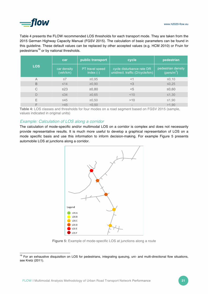
Table 4 presents the FLOW recommended LOS thresholds for each transport mode. They are taken from the 2015 German Highway Capacity Manual (FGSV 2015). The calculation of basic parameters can be found in this guideline. These default values can be replaced by other accepted values (e.g. HCM 2010) or Fruin for pedestrians16 or by national thresholds.

LOS

car public transport cycle pedestrian

car density (veh/km)

PT travel speed index (-)

cycle disturbance rate DR unidirect. traffic (D/cycle/km)

pedestrian density (pers/m2)

A ≤7 ≥0,95 <1 ≤0,10 B ≤14 ≥0,90 <3 ≤0,25 C ≤23 ≥0,80 <5 ≤0,60 D ≤34 ≥0,65 <10 ≤1,30

E ≤45 ≥0,50 >10 ≤1,90 F >45 <0,50 - >1,90

Table 4: LOS classes and thresholds for four modes on a road segment based on FGSV 2015 (sample, values indicated in original units)

Example: Calculation of LOS along a corridor The calculation of mode-specific and/or multimodal LOS on a corridor is complex and does not necessarily provide representative results. It is much more useful to develop a graphical representation of LOS on a mode specific basis and use this information to inform decision-making. For example Figure 5 presents automobile LOS at junctions along a corridor.

Figure 5: Example of mode-specific LOS at junctions along a route

16 For an exhaustive disquisition on LOS for pedestrians, integrating queuing, uni- and multi-directional flow situations, see Kretz (2011).

www.h2020-flow.eu


By presenting corridor LOS in this manner, the calculation and assignment of LOS values by mode can be displayed for all four transport modes separately, based on the specific values used to calculate LOS for that particular mode.

Transforming LOS classes into utility points

FLOW is developing a single multimodal measure of transport network service quality by aggregating individual mode-specific measurements. In order to provide a common basis for the aggregation, the six LOS classes are converted into utility points using a discrete utility function that ranges from 0 to 120. In this approach, utility points are set as a mean of the corresponding quality classes since values for the six LOS classes vary among the different modes (Table 5).

LOS utility points range of utility points A 110 101-120 B 90 81-100

C 70 61-80 D 50 41-60

E 30 21-40

F 10 1-20 Table 5: Transformation of LOS classes into utility points

The utility points are uniformly distributed across the six LOS thresholds. Therefore, the difference between LOS A and LOS B is equal to the difference between LOS E and LOS F, as shown in column 2 of Table 5. In order to aggregate the utility points, which are computed by mode, into a single aggregated utility value, a mean utility point is computed as a weighted average (see chapter 3.2) of all utility points by mode. These mean utility points can then be converted into an integrated level of service (for all modes) by associating the results with the utility classes (column 3). The aggregation process is described in the following section.

3.4. Aggregation of mode-specific KPIs into a multimodal performance index (MPI)

FLOW’s multimodal performance index (MPI) for transport network service quality is calculated by aggregating mode-specific KPIs for delay and LOS (an aggregated KPI for density is not created because, as outlined in chapter 3.3.2, this would result in a loss of significance of the measurement). Aggregated multimodal delay and LOS are theoretical values which represent the efficiency of a network element considering all modes. The current mono-modal understanding of transport network performance (i.e. congestion) focuses solely on high densities or significant delays for motor vehicles, and therefore neglects available infrastructure capacity for non-motorised transport. In contrast, the aggregated multimodal approach points out the multimodal transport system’s capacity reserve. In addition to aggregating individual mode-specific KPIs into a single MPI, the FLOW methodology enables decision-makers to adjust KPI calculation parameters to be consistent with their city’s strategic objectives (e.g. promotion of cycling or walking). Table 6 summarises the weighting values proposed by FLOW in accordance with the assessment levels described in chapter 3.1.

www.h2020-flow.eu


Table 6: Different aggregation possibilities offered by FLOW17

The weighting options presented in Table 6 enable cities to incorporate their strategic transport objectives into their KPI calculations. A combined multimodal performance index may be able to demonstrate to stakeholders and decision-makers that, when all traffic participants are fully taken into consideration, a given measure may not lead to increased congestion. City-to-city comparisons are possible when both cities apply the same weighting factors; when cities use different weighting factors, their final results cannot be directly compared. While the separate consideration of LOS for each transport mode is necessary for analysis, use of the aggregated multimodal measurement is only required if KPIs are needed for more than one mode. A pre-requisite for aggregation (and comparison) is a common base. The FLOW methodology provides this through mode-specific variables in the same units. These are:

• Delay – person-based delay values for all means of transport • LOS – utility points for different mode-specific LOS classes

The calculation procedures for these indicators are described in chapters 3.3.1. to 3.3.3. In addition to this, the mode-specific traffic volumes are transformed from veh/h into persons/h by means of mode- and purpose-specific vehicle occupancy ratios. In this case car occupancy is estimated based on trip purpose, whereas public transport occupancy is determined by vehicle capacity and use. A vehicle occupancy ratio of 1 is assumed for bicycles; however, trip purpose adaptation may be necessary in order to account for the transport of children in trailers or cargo bikes. The transformation of pedestrians is not required. The mode-specific vehicle occupancy ratios are determined by each city. The aggregated mean multimodal indicators are calculated using the following formula:

𝑀𝑃𝐼 =𝐾𝑃𝐼!,! ∙ 𝑞!,! ∙ 𝑝!!

!!!!!!!

𝑞!,!!!!! ∙ 𝑝!!

!!!

Where MPI = mean multimodal performance index (delay [s/pers] or LOS utility points [UP]) KPIj,i = key performance indicator on a network element i for transport mode j [s/pers or UP] n = number of transport modes [-] k = number of relevant turning movements (at a junction) [-] qj,j = mode specific traffic volume on network element i for transport mode j [pers/h] pj = priority factor for transport mode j [-], set by the city

17 Aggregation and transformation are carried out for delay and LOS but not for density as this leads to a loss of significance according to traffic engineering. See chapter 3.3 for details.

local network

delay [s/person]

td,i,j = mean delay on lane i for transport mode j

td,j = transport mode specific delay along the whole corridor for transport mode j

LOS [A-F]

UPi,j = utility point on lane i for transport mode j

Only graphical display of single values

Weighting factor based on city strategy

prioritised transport mode: qi,j (pers/h); pj (-)no priority, only single weighting: qi,j (pers/h); pj = 1all transport modes are treated equally: qi,j = 1 pj = 1

KPIInput variable after transformation

depending on scale of measure

www.h2020-flow.eu


The use of utility points is a fundamental part of the KPI for LOS since they better reflect the perceptions of different traffic participants (e.g. the difference between a car driver and a bike rider). LOS utility points are aggregated by means of the formula described above. As an additional step, this utility point is “transformed back” and assigned to an LOS class (see classes in Table 5 in chapter 3.3.3). A graphical display with a single aggregated multimodal junction or segment value can also be provided for level of service.

4. Determination of multimodal congestion threshold

In the FLOW context, the role of multimodal KPIs is to describe the multimodal performance of an urban road transport network by treating all transport modes equally. For this evaluation, the KPIs are calculated either as single, mode-specific variables or as an aggregated, multimodal abstract value (MPI). Once a city has calculated values for these KPIs, it is possible to set a threshold value beyond which conditions are considered unacceptable, and therefore “congested”. This reference point is the congestion threshold (see chapter 2 for the FLOW definition of multimodal transport network performance and congestion). Congestion thresholds can be defined in two ways: either based on continuous values (an element of the urban road network is perceived to be congested if the density or the delay per traffic participant exceeds a specified value), or based on discrete classes. The latter approach typically corresponds to LOS classification: the most common process aims to evaluate multimodal road transport network performance, thus defining congestion based on assigned LOS categories. Cities must determine their own congestion thresholds (the point beyond which traffic conditions are considered unacceptable) and, as such setting this threshold represents a political decision. The threshold represents the point at which the city believes intervention is required. Since the threshold is determined by individual cities, there will be variation from city to city and from transport mode to transport mode based on local perceptions and different policy objectives. As with the priority setting in chapter 3.2, the threshold can be established based on policy priorities formulated in a sustainable urban mobility planning process. The standard traffic engineering references all recognise that it is virtually impossible to provide high levels of LOS in peak periods and therefore recommend LOS D or even LOS E as acceptable during these periods. For example, according to the US HCM: LOS D “is a common goal for urban streets during peak hours, as attaining LOS C would require prohibitive cost and societal impact in bypass roads and lane additions (…). LOS E is a common standard in larger urban areas, where some roadway congestion is inevitable.” Furthermore, recent research (Newton and Curry 2014) is questioning the whole idea of using LOS and other congestion based methods for evaluating transport network performance because it leads to an overemphasise on roadway construction and does not fully incorporate the notion of induced traffic.

www.h2020-flow.eu


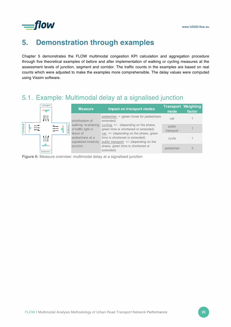
5. Demonstration through examples Chapter 5 demonstrates the FLOW multimodal congestion KPI calculation and aggregation procedure through five theoretical examples of before and after implementation of walking or cycling measures at the assessment levels of junction, segment and corridor. The traffic counts in the examples are based on real counts which were adjusted to make the examples more comprehensible. The delay values were computed using Vissim software.

5.1. Example: Multimodal delay at a signalised junction

Figure 6: Measure overview: multimodal delay at a signalised junction

Measure Impact on transport modes Transport mode

Weighting factor

car 1

public transport

1

cycle 1

pedestrian 3

pedestrian: + (green times for pedestrians extended)cycling: +/- (depending on the phase, green time is shortened or extended)car: +/- (depending on the phase, green time is shortened or extended)public transport: +/- (depending on the phase, green time is shortened or extended)

prioritisation of walking: re-phasing of traffic light in favour of pedestrians at a signalised innercity junction

www.h2020-flow.eu


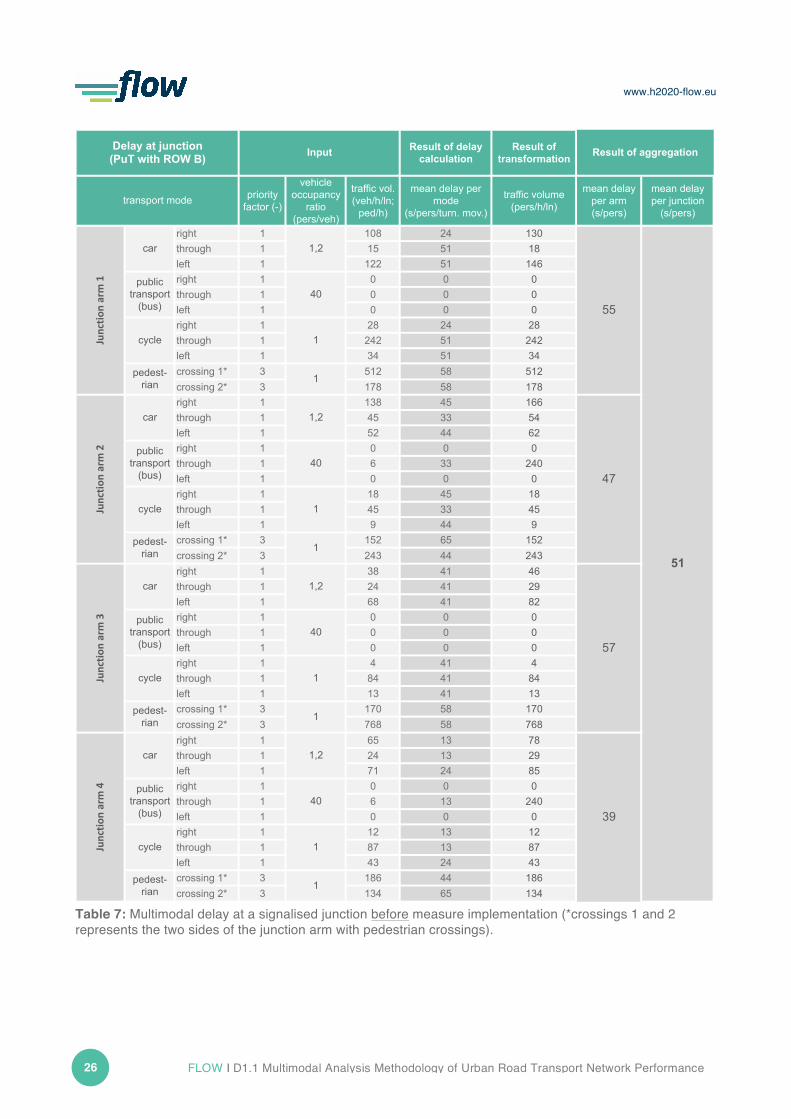
Table 7: Multimodal delay at a signalised junction before measure implementation (*crossings 1 and 2 represents the two sides of the junction arm with pedestrian crossings).

Result of delay calculation

Result of transformation

priority factor (-)

vehicle occupancy

ratio (pers/veh)

traffic vol. (veh/h/ln;

ped/h)

mean delay per mode

(s/pers/turn. mov.)

traffic volume(pers/h/ln)

mean delay per arm (s/pers)

mean delay per junction

(s/pers)

right 1 108 24 130through 1 15 51 18left 1 122 51 146right 1 0 0 0through 1 0 0 0left 1 0 0 0right 1 28 24 28through 1 242 51 242left 1 34 51 34crossing 1* 3 512 58 512crossing 2* 3 178 58 178right 1 138 45 166through 1 45 33 54left 1 52 44 62right 1 0 0 0through 1 6 33 240left 1 0 0 0right 1 18 45 18through 1 45 33 45left 1 9 44 9crossing 1* 3 152 65 152crossing 2* 3 243 44 243right 1 38 41 46through 1 24 41 29left 1 68 41 82right 1 0 0 0through 1 0 0 0left 1 0 0 0right 1 4 41 4through 1 84 41 84left 1 13 41 13crossing 1* 3 170 58 170crossing 2* 3 768 58 768right 1 65 13 78through 1 24 13 29left 1 71 24 85right 1 0 0 0through 1 6 13 240left 1 0 0 0right 1 12 13 12through 1 87 13 87left 1 43 24 43crossing 1* 3 186 44 186crossing 2* 3 134 65 134

40

Input

1,2

1,2

Delay at junction(PuT with ROW B)

transport mode

pedest-rian 1

Junctio

n(arm(1

car

cycle

public transport

(bus)

Result of aggregation

55

51

57

39

1

40

1

40

1

cycle

public transport

(bus)

cycle

public transport

(bus)

pedest-rian

car

Junctio

n(arm(3

car

Junctio

n(arm(2

car

pedest-rian

pedest-rian

47

1,2

1,2

cycle

public transport

(bus)

40

1

Junctio

n(arm(4

1

1

1

www.h2020-flow.eu


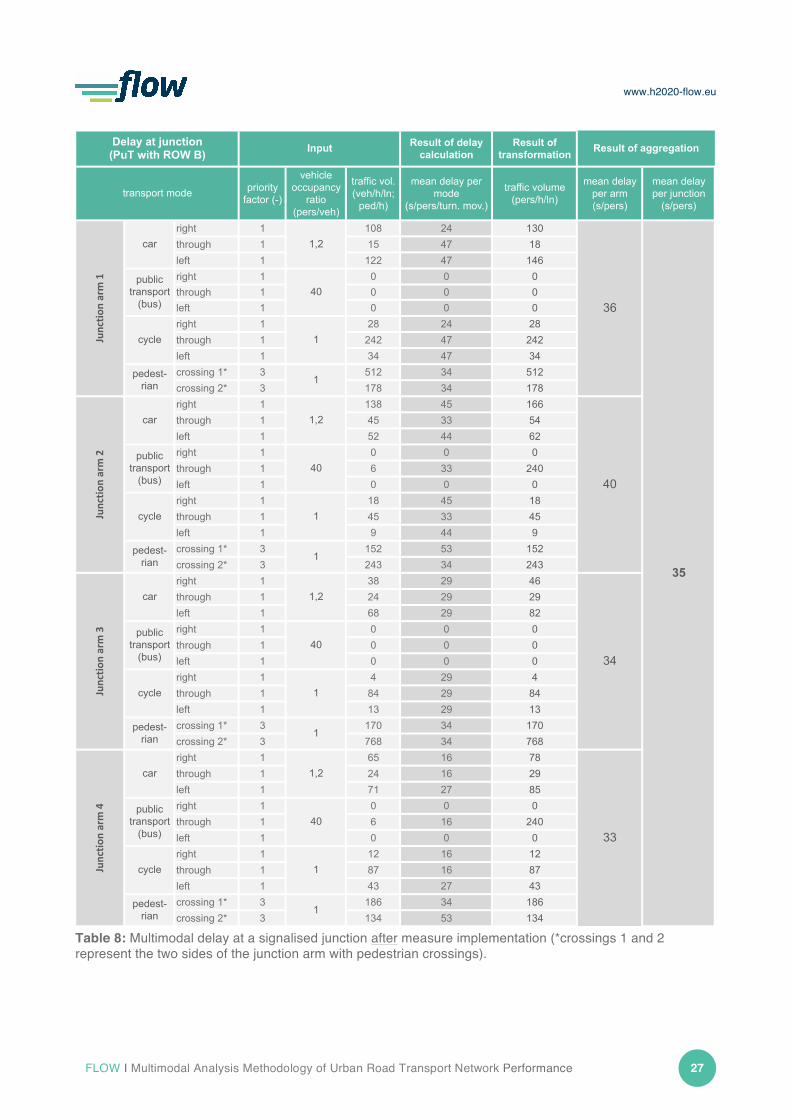
Table 8: Multimodal delay at a signalised junction after measure implementation (*crossings 1 and 2 represent the two sides of the junction arm with pedestrian crossings).



priority factor (-)

vehicle occupancy

ratio (pers/veh)

traffic vol. (veh/h/ln;

ped/h)

mean delay per mode

(s/pers/turn. mov.)

traffic volume(pers/h/ln)

mean delay per arm (s/pers)

mean delay per junction

(s/pers)

right 1 108 24 130through 1 15 47 18left 1 122 47 146right 1 0 0 0through 1 0 0 0left 1 0 0 0right 1 28 24 28through 1 242 47 242left 1 34 47 34crossing 1* 3 512 34 512crossing 2* 3 178 34 178right 1 138 45 166through 1 45 33 54left 1 52 44 62right 1 0 0 0through 1 6 33 240left 1 0 0 0right 1 18 45 18through 1 45 33 45left 1 9 44 9crossing 1* 3 152 53 152crossing 2* 3 243 34 243right 1 38 29 46through 1 24 29 29left 1 68 29 82right 1 0 0 0through 1 0 0 0left 1 0 0 0right 1 4 29 4through 1 84 29 84left 1 13 29 13crossing 1* 3 170 34 170crossing 2* 3 768 34 768right 1 65 16 78through 1 24 16 29left 1 71 27 85right 1 0 0 0through 1 6 16 240left 1 0 0 0right 1 12 16 12through 1 87 16 87left 1 43 27 43crossing 1* 3 186 34 186crossing 2* 3 134 53 134

36

Delay at junction(PuT with ROW B) Input Result of aggregation

transport mode

car 1,2

40

1

34

public transport

(bus)40

cycle 1

cycle

public transport

(bus)40

cycle 1

pedest-rian

Junctio

n(arm(3

car 1,2

1

Junctio

n(arm(1

car 1,2

Junctio

n(arm(2 public

transport (bus)

40

1

pedest-rian

Junctio

n(arm(4

car 1,2

pedest-rian 1

33

public transport

(bus)40

cycle 1

pedest-rian 1

35

www.h2020-flow.eu


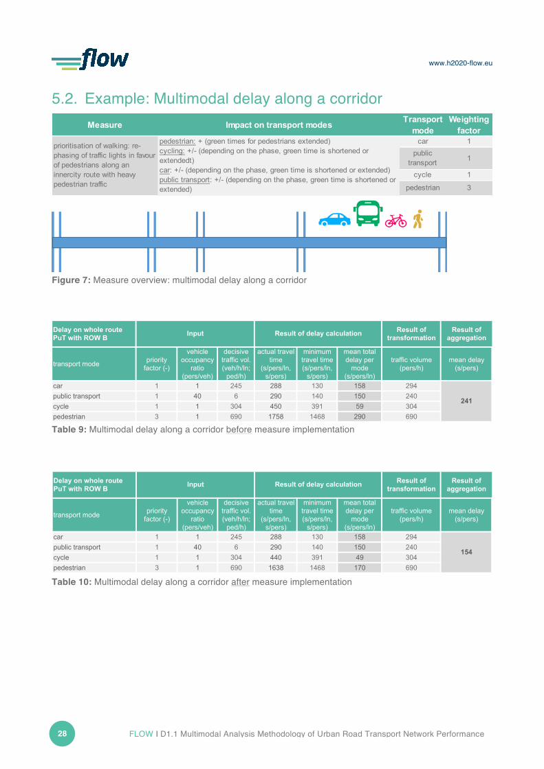
5.2. Example: Multimodal delay along a corridor

Figure 7: Measure overview: multimodal delay along a corridor

Table 9: Multimodal delay along a corridor before measure implementation

Table 10: Multimodal delay along a corridor after measure implementation


Weighting factor

car 1public

transport 1

cycle 1

pedestrian 3

prioritisation of walking: re-phasing of traffic lights in favour of pedestrians along an innercity route with heavy pedestrian traffic

pedestrian: + (green times for pedestrians extended)cycling: +/- (depending on the phase, green time is shortened or extendedt)car: +/- (depending on the phase, green time is shortened or extended)public transport: +/- (depending on the phase, green time is shortened or extended)

Delay on whole routePuT with ROW B



transport mode priority factor (-)

vehicle occupancy

ratio (pers/veh)

decisive traffic vol. (veh/h/ln;

ped/h)

actual travel time

(s/pers/ln, s/pers)

minimum travel time (s/pers/ln,

s/pers)

mean total delay per

mode (s/pers/ln)

traffic volume (pers/h)

mean delay (s/pers)

car 1 1 245 288 130 158 294public transport 1 40 6 290 140 150 240cycle 1 1 304 450 391 59 304pedestrian 3 1 690 1758 1468 290 690


241

Input

Delay on whole routePuT with ROW B



transport mode priority factor (-)

vehicle occupancy

ratio (pers/veh)

decisive traffic vol. (veh/h/ln;

ped/h)

actual travel time

(s/pers/ln, s/pers)

minimum travel time (s/pers/ln,

s/pers)

mean total delay per

mode (s/pers/ln)


mean delay (s/pers)

car 1 1 245 288 130 158 294public transport 1 40 6 290 140 150 240cycle 1 1 304 440 391 49 304pedestrian 3 1 690 1638 1468 170 690

Input Result of delay calculation

154

www.h2020-flow.eu


5.3. Example: Multimodal density on road segment

Figure 8: Measure overview: multimodal density on road segment (transformation and aggregation of single mode-specific density values is not required).

Table 11: Multimodal density on a road segment before measure implementation (*sidewalk width: 2 m, effective width: 1.05 m).

Table 12: Multimodal density on a road segment after measure implementation (* sidewalk width: 5 m (effective width: 4.05 m).

Measure Impact on transport modes

Transport mode

Weighting factor

car 1

cycle 1

pedestrian 2

prioritisation of walking: widening of sidewalk in favour of pedestrians

pedestrian: + (width of pavement doubled)cycling: 0 (no change)car: - (one lane taken away)

Density on road segment Result of density calculation

transport modepriority factor

(-)

traffic volume (veh/h/ln,

ped/h)

average travel speed (km/h)

density per mode (veh/km, ped/km )

car 1 125 23 5cycle 1 200 12 17pedestrian* 2 1850 4 872

Input

Density on road segment Result of density calculation


(-)


ped/h)

average travel speed (km/h)

density per mode (veh/km, ped/km )

car 1 250 21 12

cycle 1 200 12 17

pedestrian* 2 1850 4 770

Input

www.h2020-flow.eu


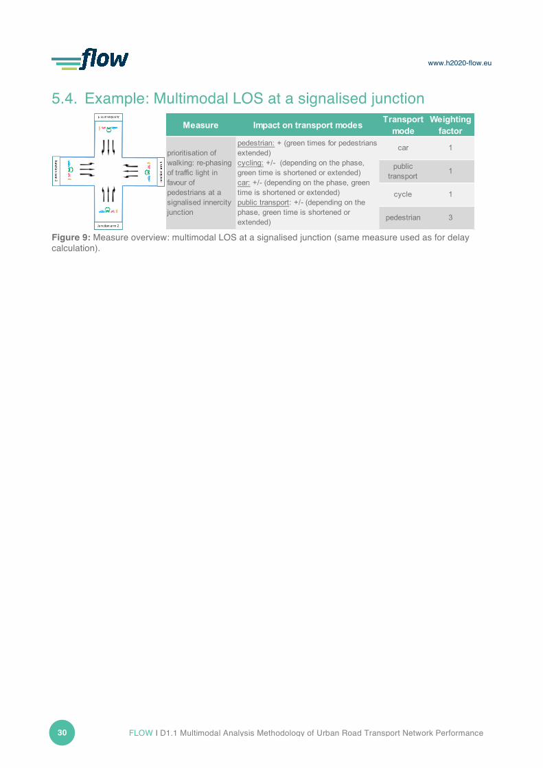
5.4. Example: Multimodal LOS at a signalised junction

Figure 9: Measure overview: multimodal LOS at a signalised junction (same measure used as for delay calculation).


Weighting factor

car 1

public transport

1

cycle 1

pedestrian 3

pedestrian: + (green times for pedestrians extended)cycling: +/- (depending on the phase, green time is shortened or extended)car: +/- (depending on the phase, green time is shortened or extended)public transport: +/- (depending on the phase, green time is shortened or extended)

prioritisation of walking: re-phasing of traffic light in favour of pedestrians at a signalised innercity junction

www.h2020-flow.eu


Table 13: Multimodal LOS at a junction before measure implementation

Result of LOS

calculation

priority factor (-)

vehicle occupancy ratio (pers/veh)

traffic vol. (veh/h/ln; ped/h)

LOSutility points

UP (-)traffic volume

(pers/h) mean utility (-) mean LOS

right 1 108 B 90 130through 1 15 D 50 18left 1 122 D 50 146right 1 - - - -through 1 - - - -left 1 - - - -right 1 28 A 110 28through 1 242 C 70 242left 1 34 C 70 34crossing 1* 3 512 D 50 512crossing 2* 3 178 D 50 178right 1 138 C 70 166through 1 45 B 90 54left 1 52 C 70 62right 1 - - - -through 1 6 D 50 240left 1 - - - -right 1 18 C 70 18through 1 45 B 90 45left 1 9 C 70 9crossing 1* 3 152 D 50 152crossing 2* 3 243 C 70 243right 1 38 C 70 46through 1 24 C 70 29left 1 68 C 70 82right 1 - - - -through 1 - - - -left 1 - - - -right 1 4 C 70 4through 1 84 C 70 84left 1 13 C 70 13crossing 1* 3 170 D 50 170crossing 2* 3 768 D 50 768right 1 65 A 110 78through 1 24 A 110 29left 1 71 B 90 85right 1 - - - -through 1 6 B 90 240left 1 - - - -right 1 12 A 110 12through 1 87 A 110 87left 1 43 A 110 43crossing 1* 3 186 C 70 186crossing 2* 3 134 D 50 134


59 D


Junctio

n arm 4

car 1,2

public transport

(bus)40

cycle 1

pedest-rian 1

Junctio

n arm 3

car 1,2

public transport

(bus)40

cycle 1

pedest-rian 1

40

cycle 1

pedest-rian 1

Junctio

n arm 2

car 1,2

public transport

(bus)

LOS at a junction(PuT with ROW B) Input

transport mode

Junctio

n arm 1

car 1,2

public transport

(bus)40

cycle 1

pedest-rian 1

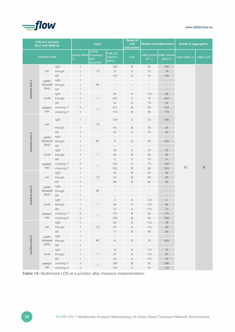
www.h2020-flow.eu


Table 14: Multimodal LOS at a junction after measure implementation

Result of LOS

calculation

priority factor (-)

vehicle occupancy ratio (pers/veh)

traffic vol. (veh/h/ln; ped/h)

LOSutility points

UP (-)traffic volume

(pers/h) mean utility (-) mean LOS

right 1 108 B 90 130through 1 15 C 70 18left 1 122 C 70 146right 1 - - - -through 1 - - - -left 1 - - - -right 1 28 A 110 28through 1 242 C 70 242left 1 34 C 70 34crossing 1* 3 512 B 90 512crossing 2* 3 178 B 90 178

right 1 138 C 70 166

through 1 45 B 90 54left 1 52 C 70 62right 1 - - - -through 1 6 D 50 240left 1 - - - -right 1 18 C 70 18through 1 45 B 90 45left 1 9 C 70 9crossing 1* 3 152 C 70 152crossing 2* 3 243 B 90 243right 1 38 B 90 46through 1 24 B 90 29left 1 68 B 90 82right 1 - - - -through 1 - - - -left 1 - - - -right 1 4 A 110 4through 1 84 A 110 84left 1 13 A 110 13crossing 1* 3 170 B 90 170crossing 2* 3 768 B 90 768right 1 65 A 110 78through 1 24 A 110 29left 1 71 B 90 85right 1 - - - -through 1 6 C 70 240left 1 - - - -right 1 12 A 110 12through 1 87 A 110 87left 1 43 A 110 43crossing 1* 3 186 B 90 186crossing 2* 3 134 C 70 134

Junctio

n arm 4

car 1,2

public transport

(bus)40

cycle 1

pedest-rian 1

Junctio

n arm 3

car 1,2

public transport

(bus)40

cycle 1

pedest-rian 1

40

cycle 1

pedest-rian 1

LOS at a junction(PuT with ROW B) Input

transport mode

Junctio

n arm 1

car 1,2

public transport

(bus)40

cycle 1

pedest-rian 1


86 B


Junctio

n arm 2

car 1,2

public transport

(bus)

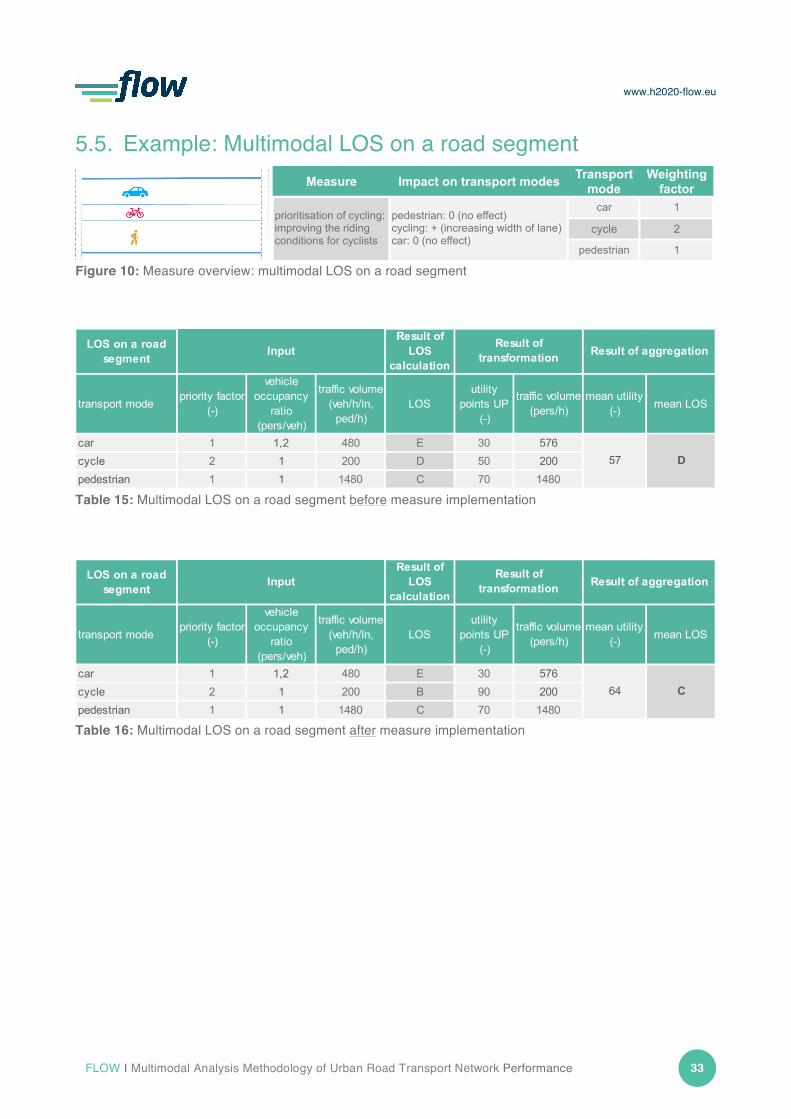
www.h2020-flow.eu


5.5. Example: Multimodal LOS on a road segment

Figure 10: Measure overview: multimodal LOS on a road segment

Table 15: Multimodal LOS on a road segment before measure implementation

Table 16: Multimodal LOS on a road segment after measure implementation


Weighting factor

car 1

cycle 2

pedestrian 1

cyclepedestrian

After

LOS on a road segment

transport mode

carcyclepedestrian

prioritisation of cycling: improving the riding conditions for cyclists

pedestrian: 0 (no effect)cycling: + (increasing width of lane)car: 0 (no effect)


Result of LOS

calculation


(-)

vehicle occupancy

ratio (pers/veh)


ped/h) LOS

utility points UP

(-)


mean utility (-) mean LOS

car 1 1,2 480 E 30 576cycle 2 1 200 D 50 200pedestrian 1 1 1480 C 70 1480

57 D

Input Result of transformation Result of aggregation


Result of LOS

calculation


(-)

vehicle occupancy

ratio (pers/veh)


ped/h) LOS

utility points UP

(-)


mean utility (-) mean LOS

car 1 1,2 480 E 30 576cycle 2 1 200 B 90 200pedestrian 1 1 1480 C 70 1480

64 C

Input Result of transformation Result of aggregation

www.h2020-flow.eu


6. Achievements, limitations and outlook

6.1. Achievements The FLOW project has developed a methodology for analysing transport network performance from a multimodal perspective. The process began with the development of a multimodal definition of congestion (in contrast to existing definitions that focus on motor vehicles) that includes the user perspective and allows for adaptability to local circumstances. This definition is operationalised through the development of KPIs designed to better reflect all modes of transport and to overcome the limitations of current mono-modal evaluation techniques. The proposed methodology consists of:

1. calculating the performance and capacity of each transport mode independently: the formulas for these mode-specific calculations were taken from recent technical guidelines and capacity manuals in order to ensure technical consistency. In addition, the KPI ‘delay’ is evaluated on a person basis rather than a vehicle basis (following the premise of moving people, as opposed to vehicles).

2. offering an aggregation procedure to create a multimodal performance index: the MPI provides a single value that represents the transport system as a whole at the selected network assessment level. This aggregation emphasises the importance of a multimodal transport system and shows, through the aggregation of mode-specific KPIs, the implementation of a specified measure does not necessarily lead to more congestion if all traffic participants are taken into account.

3. providing the option to apply a weighting in the aggregation process so that the index can be adjusted to reflect the strategic priorities of a city.

Developing a truly multimodal method for assessing transport system performance is an extremely ambitious task both conceptually and technically. Furthermore, there is a huge disconnect between traffic engineering and transport planning in terms of language, understanding and objectives. While the FLOW methodology is an improvement upon current methods, it clearly has limitations due to its ambitiousness and the professional disconnect. The next section describes some of those limitations and makes recommendations for addressing them. One final point: the FLOW project, by bringing together traffic engineers and transport planners is an important step in bridging the disconnect between these professions. Moreover, not only transport professionals but also decision-makers, local stakeholders and citizens will be involved in understanding the findings of the FLOW project. This work will continue through the project and into the future – this is one of the project’s key successes.

6.2. Limitations This section outlines the key limitations of the proposed FLOW methodology and makes recommendations for addressing these limitations in future research.

www.h2020-flow.eu


6.2.1. Applicability on shared elements of the urban road transport network A key limitation of the FLOW methodology is that it can only be directly applied to those parts of the urban road transport network where traffic lanes are used by a single transport mode. Thus the following interactions can NOT be evaluated:

• interactions between different modes within a shared lane (e.g. cars and bikes share a lane; the volume of each varies depending on a range of factors)

• situations where mutual disturbance is caused by lateral movement of vehicles, cyclists or pedestrians from their own designated space into the neighbouring space due to crowding in their space (e.g. a cyclist leaves the cycle lane while overtaking and disturbs motorised traffic in the adjacent lane; pedestrians spill out onto the roadway when the sidewalk is extremely crowded);

The interaction of different transport modes within the same space is highly complex. Research is being done on this topic and new models are being developed. A good example is the complete streets research being done in the United States. In addition to this large-scale transport planning research specific research to help develop more appropriate shared facility evaluation techniques include:

• behavioural research to gather data on different capacity concepts that are influenced by modal interrelations

• development of capacity and density calculation methodologies to better consider interactions between modes on the urban road network and especially shared lanes

In short, the field of developing shared facility transport analysis for multimodal planning is undergoing rapid change and these will provide many opportunities for improving the FLOW methodology in future projects.

6.2.2. Understanding of perception of delay for users of different transport modes

While FLOW aims to address user perceptions of transport network performance, the operationalised KPIs cannot fully reflect the spatial, temporal and personal variations in user perception described in the FLOW definition of multimodal transport network performance. As noted in chapter 2, not enough is known about the perception of delay for users of different modes of transport. Further research on acceptable (as opposed to minimum) travel time for all modes would serve to replace the easily calculated – but oversimplified – proxy of minimum travel time. This research would have to account for the fact that expectations change as the service quality change – people adjust to the new normal.

6.2.3. Moving people, not vehicles

One of the key principles of modern transport planning is “moving people, not vehicles”. Therefore in developing the FLOW methodology we attempted to calculate KPIs in terms of moving people. This was possible for the KPI ‘delay’ but not possible for the KPI ‘density’ for technical reasons. Additional basic research could be done to develop a more person-based method for calculating density.

Another, perhaps more promising approach, would be to develop a new KPI that truly captures the idea underling the principle of “moving people, not vehicles”. The FLOW project results can form the basis for this sort of very basic research combining traffic engineering and transport planners – in part simply because it has raised the question and brought the interested parties together to work on developing a common understanding of transport network performance.

www.h2020-flow.eu


6.2.4. Understanding of network-wide multimodal LOS Another limitation of the FLOW methodology is that it does not provide common approach to assessing mode-specific LOS values. It uses different basic variables to evaluate the service quality experienced by different traffic participants. Furthermore, these LOS classes are not linearly distributed and the different LOS levels are interpreted in different ways for each mode. Therefore the LOS measures for different modes cannot equally describe the quality of service experienced by traffic participants. More specifically, while the car and public transport LOS measures are directly linked to the perceived attractiveness of these modes, there is less evidence of this relationship for the walking and cycling LOS measures. For example, a pedestrian segment (e.g. a shopping street) experiencing a “low” service quality (e.g. LOS ‘E’ or ‘F’) on a Saturday afternoon may be perceived as attractive, whereas an arterial road experiencing a LOS ‘E’ or ‘F’ on a weekday morning is rarely considered attractive. The inability to fully integrate the perceptions of different traffic participants leads to an inevitable loss of individual preferences during the aggregation to an average LOS. Some specific research that could help address the limitation of having a true multimodal measure for LOS include:

• Developing new methods for determining LOS using the same variables for each transport mode (rather than having to rely on a conversion to utility points);

• Studying how to refine the FLOW methodology’s aggregation procedure and extending it to an average network-wide multimodal LOS;

• Developing an integral method for assigning aggregated mean multimodal KPI (density or delay) to LOS, instead of providing single LOS values for each mode and then aggregating them in a second step;

• Conducting behaviour research to identify LOS measures for walking and cycling that better reflect the attractiveness, safety and comfort of these modes as perceived by users.

Again, while the FLOW methodology has the limitation of not being able to calculate a fully consistent LOS for all modes, it represents an improvement over monomodal methods in the sense that it is multimodal. Furthermore, the FLOW project has clearly identified the need for more research on this subject and outlined possible methods for completing this research.

6.3. Outlook The FLOW methodology will be applied by technical staff in the FLOW Partner Cities of Budapest, Dublin, Gdynia, Lisbon and Munich to analyse the effect of selected cycling and walking measures on the transport network performance of each city. The results of the application of the methodology will serve as input for the analysis of broader impacts of given walking and cycling measures on urban road transport network performance through an impact assessment tool which is also being developed within the FLOW project.18

The results of applying the FLOW methodology are intended to initiate a more informed debate among technical staff, decision makers and the public in the FLOW partner cities. These can serve as examples to other cities wishing to apply multimodality when planning and analysing their urban road transport network. 18 For the latest information on other FLOW activities and products, please sign up to the FLOW newsletter at www.h2020-flow.eu.

www.h2020-flow.eu


7. References Adomaitis, K. (2014). The Rise of Cycling Cities in Europe. Available at http://blog.euromonitor.com/2014/09/the-rise-of-cycling-cities-in-europe.html. Börjesson, Maria and J. Eliasson (2012). The Value of Time and External Benefits in Bicycle Appraisal. In: Transportation Research Part A 46 (2012) 673-683. Bovy, P.H.L. and I. Salomon (2002). Congestion in Europe: Measurements, Patterns and Policies. In: E. Stern, I. Salomon, P.H.L. Bovy (Eds). Travel Behaviour: Spatial Patterns, Congestion and Modelling, pp. 143-179. Cheltenham. Buehler, Ralph and J. Pucher (2012). Walking and Cycling in Western Europe and the United States: Trends, Policies and Lessons. TR News 280. May-June 2012. Available at http://onlinepubs.trb.org/onlinepubs/trnews/trnews280WesternEurope.pdf. Dowling, Richard, D. Reinke, A. Flannery, P. Ryus, M. Vandehey, T. Petritsch, B. Landis, N. Rouphail, J. Bonneson (2008). Multimodal Level of Service Analysis for Urban Streets. NCHRP Report 616. Transportation Research Board. Washington D.C. Available at http://onlinepubs.trb.org/onlinepubs/nchrp/nchrp_rpt_616.pdf. European Conference of Ministers of Transport (2007). Managing Urban Traffic Congestion. OECD/ECMT. Available at: http://www.internationaltransportforum.org/Pub/pdf/07Congestion.pdf. FGSV - Forschungsgesellschaft für Straßen- und Verkehrswesen (2015). Handbuch für die Bemessung von Straßenverkehrsanlagen (HBS) Teil S Stadtstraßen. FGSV Verlag Köln. Fruin, John J. (1971). Pedestrian Planning and Design. Metropolitan Association of Urban Designers and Environmental Planners. New York. Kretz, Tobias (2011). A Level of Service Scheme for Microscopic Simulation of Pedestrians that Integrates Queuing, Uni- and Multi-Directional Flow Situations. In: European Transport Research Review December 2011, Volume 3, Issue 4, pp 211-220. Available at http://link.springer.com/article/10.1007/s12544-011-0060-7/fulltext.html. Lighthill, M. J. and G. B. Whitham (1955). On Kinematic Waves. II. A Theory of Traffic Flow on Long Crowded Roads. Available at https://amath.colorado.edu/sites/default/files/2013/09/1710796241/PRSA_Lighthill_1955.pdf. Litman, Todd (2016). Smart Congestion Relief. Comprehensive Evaluation of Traffic Congestion Costs and Congestion Reduction Strategies. Victoria Transport Policy Institute. Available at http://www.vtpi.org/cong_relief.pdf. Malmö Stad (2016). Sustainable Urban Mobility Plan: Creating a More Accessible Malmö. Malmö.

www.h2020-flow.eu


Newton, D. and Curry, M. (2014) California has officially ditched car-centric “Level of Service”. Available online: http://la.streetsblog.org/2014/08/07/california-has-officially-ditched-car-centric-level-of-service/ Pooley, Colin, D. Horton, G. Scheldeman, C. Mullen, T. Jones, M. Tight, A. Jopson, A. Chisholm (2013). Policies for Promoting Walking and Cycling in England: A View from the Street. Transport Policy 27 (2013) 66-72. PTV Planung Transport Verkehr AG (2011). PTV Vissim 8. User Manual. PTV AG, Karlsruhe. Stopher, P. R. (2004). Reducing Road Congestion: A Reality Check. Transport Policy 11 (2004) 117-131. TRB - Transport Research Board (2010). Highway Capacity Manual 2010. National Research Council, Washington, D.C. United Kingdom Department for Transport (2001). Perceptions of and Attitudes to Congestion, http://webarchive.nationalarchives.gov.uk/20031216140150/http://www.odpm.gov.uk:80/stellent/groups/dft_transstats/documents/pdf/dft_transstats_pdf_505810.pdf. Urban Movement, Phil Jones Associates (2014). International Cycling Infrastructure Best Practice Study (Appendix). Available at http://content.tfl.gov.uk/international-cycling-infrastructure-best-practice-study-appendix.pdf.

Weisbrod, Glen, D. Vary, G. Treyz (2001). Economic Implications of Congestion. In: National Cooperative Highway Research Program Report 463, Transportation Research Board, Washington, DC. http://onlinepubs.trb.org/Onlinepubs/nchrp/nchrp_rpt_463-a.pdf Woodcock, James, P. Edwards, C. Tonne, B. G. Armstrong, O. Ashiru, D. Banister, S. Beevers, Z. Chalabi, Z. Chowdhury, A. Cohen, O. H. Franco, A. Haines, R. Hickman, G. Lindsay, I. Mittal, D. Mohan, G. Tiwari, A. Woodward and I. Roberts (2009). Public Health Benefits of Strategies to Reduce Greenhouse-Gas Emissions: Urban Land Transport, www.thelancet.com, Vol 374, pp. 1930-1943, December 5, 2009.

www.h2020-flow.eu


Multimodal Analysis Methodology of Urban Road Transport...

Documents

Transcript of Multimodal Analysis Methodology of Urban Road Transport...