IEEE TRANSACTIONS ON MAGNETICS, VOL. 50, NO. 2, FEBRUARY 2014 7000404

Multilevel Preconditioning for Time-Harmonic Eddy-CurrentProblems Solved With Hierarchical Finite Elements

Ali Aghabarati and Jon P. Webb

Department of Electrical and Computer Engineering, McGill University, Montreal, QC H3A 0E9, Canada

A multilevel preconditioner is described for high-order finite element analysis of eddy currents using the T − � formulation. Thepreconditioner combines p-type multiplicative Schwartz for the higher order degrees of freedom and auxiliary space preconditioningfor the lowest order. Algebraic multigrid is applied to the first-order scalar spaces. The new preconditioner performs four timesfaster than a standard preconditioner on a test problem with 13.3 million unknowns.

Index Terms— Eddy currents, finite-element methods, multigrid methods.

I. INTRODUCTION

THREE-DIMENSIONAL eddy current problems treatedwith the finite element method (FEM) often lead to

very large matrices. Generally these are solved by Krylovsubspace iteration with a preconditioner that greatly affectsthe speed of convergence. The most common precondition-ers are based on incomplete LU (ILU) factorization or onsymmetric successive over-relaxation (SSOR). On the otherhand, multigrid preconditioners have been very successful inmany fields of engineering, particularly with scalar problems.True multigrid requires a series of nested meshes, difficultto arrange in practical problems. Algebraic multigrid (AMG)overcomes this limitation. AMG for scalar potentials is wellestablished [1]. A similar method has been applied to matricesarising from Whitney edge elements [2], [3], but for thiscase an alternative approach seems promising: auxiliary spacepreconditioning (ASP) [4], [5]. This is a way of transformingthe vector problem into a series of scalar problems, to whichAMG is well suited. In [6], ASP was applied to an eddy-current formulation that uses the magnetic vector potential.

In this paper we apply ASP to the T − � formulation.Furthermore, we consider the case that high order, hierarchicalelements [7] are used and supplement ASP with a multileveltechnique called p-type multiplicative Schwartz (pMUS) [8].

II. T−� METHOD

The phasor magnetic field H, satisfies the following equa-tions in conducting (Vc) and nonconducting (V0) subregionsof the whole problem domain, V :

∇ × σ−1 · ∇ ×H+ jωμ ·H = 0 in Vc (1a)

∇ · μ ·H = 0 in V0 (1b)

where σ and μ are the tensor conductivity and permeability,respectively. These equations are solved by the T−� method;H is represented as −∇� in V0, where � is the magnetic

Manuscript received June 14, 2013; revised August 14, 2013;accepted September 16, 2013. Date of current version February 21, 2014.Corresponding author: J. P. Webb (e-mail: jon.webb@mcgill.ca).

Color versions of one or more of the figures in this paper are availableonline at http://ieeexplore.ieee.org.

Digital Object Identifier 10.1109/TMAG.2013.2282855

scalar potential, and as T−∇� in Vc, where T is the currentvector potential. The tetrahedral finite elements in [7] are used,including the vertex functions. The rotational basis functionsrepresent T and the gradient basis functions represent ∇�. Thedecomposition is gauged by building a tree from the edges ofthe tetrahedra in the conductors; rotational functions for treeedges are omitted.

In the examples below, two different means of exciting thefield are used. In one case, � is set to a nonzero value on theboundary of V . The other method is applied when there is aprescribed net current circulating in a coil. The coil itself ispart of Vc. To make sure that the path integral of H is correctaround a loop in the air that encloses the coil current, a cutsurface is introduced in V0, spanning the coil. The potential� is made to increase by the appropriate amount in crossingthe cut surface. This jump in potential drives the field in theproblem. In both cases, application of the FEM leads to amatrix equation Ax − b.

III. p-TYPE MULTIPLICATIVE SCHWARTZ

The elements in [7] are high order and hierarchical, so thatdifferent orders can be mixed together in the same mesh,e.g., during p-adaption. Elements of orders 1–4 are used.The basis functions of the order 1 element are classified asfirst order, the functions added to take an order 1 element toorder 2 are classified as second order, and so on. All the first-order basis functions in the mesh are numbered first, then thesecond-order functions, and so on. This leads to the followingpartitioning:

A =⎡⎢⎣

A11 · · · A1p...

. . ....

A p1 · · · A pp

⎤⎥⎦ (2)

where p is the highest order present in the mesh.The pMUS preconditioner is a V-cycle that approximately

solves Ay = r , when A has this structure. The cycle consistsof a series of steps, each of which computes an improvement,�y, and updates y and r accordingly: y ← y + �y andr ← r − A�y. In the following algorithms, these updates aredenoted U(y, r). In addition, subscript l denotes a columnvector equal in size to the lth partition in (2) and Pl(r) is

0018-9464 © 2014 IEEE. Personal use is permitted, but republication/redistribution requires IEEE permission.See http://www.ieee.org/publications_standards/publications/rights/index.html for more information.

7000404 IEEE TRANSACTIONS ON MAGNETICS, VOL. 50, NO. 2, FEBRUARY 2014

the vector obtained from r by extracting its entries in the lthpartition. We start from y = 0.

For l = p, p − 1, . . . , 2

Backward GS : �yl ← Rb(All)Pl(r); U(y, r).

Solve lowest level : �y1← (A11)−1 P1(r); U(y, r).

For l = 2, 3, . . . , p

Forward GS : �yl ← R f (All)Pl(r); U(y, r).

The matrices Rb(All) and R f (All) correspond to a singlestep of backward and forward Gauss–Seidel (GS), respectively,applied to the matrix All .

In standard pMUS, the lowest level matrix problem issolved fairly accurately using either a complete or almostcomplete factorization of All [7], [8]. While it is true that theaccuracy of this step is important to the success of pMUS, forproblems with large numbers of finite elements factorizationcan be prohibitively expensive. Instead, we use ASP.

IV. AUXILIARY SPACE PRECONDITIONING

The matrix equation A11y1 = r1 is further partitioned intorows and columns corresponding to T and ∇� basis functions

[AT T AT �

A�T A��

]{yT

y�

}=

{rT

r�

}. (3)

The idea behind ASP is to transfer the problem to a numberof auxiliary function spaces. When the entire mesh is made oforder 1 elements (i.e., Whitney edge elements), two auxiliaryspaces are involved [4], [5]: the space N spanned by piecewiselinear scalar functions and the space N3 spanned by piecewiselinear vector functions, on the same mesh. In this case, thesesame auxiliary spaces are used for the T part of the field,but since this exists only inside Vc and vanishes tangentiallyon the surface, the corresponding auxiliary spaces are definedby just the nodes interior to Vc. We define matrices �n and� = [�x �y �z] that map column vectors representingfunctions in N and N3, respectively, to column vectors ofthe same size as y1 that represent T − � fields of order 1.Specifically, they map to the T partition of y1, representingfunctions in the Whitney space inside Vc. Since there are noedge functions for the tree edges in Vc, they map just to cotreeedges, but the matrix entries are the same as in [5].

The ∇� part of the field also has to be accomodated andfor this, we use the auxiliary space that is spanned by thepiecewise linear scalar functions of the whole mesh (not justthe mesh in Vc). The matrix for this space is ��. Like �n , itis a discrete representation of the gradient operator.

The ASP algorithm approximately solves A11y1 = r1 in thefollowing way, starting from y1 = 0:Backward Gauss–Seidel : �y1← Rb(A11)r1; U(y1, r1).

Initialize : �y1← 0.

For a = x, y, z, n,�

Transfer to aux. space : ra ← �Ta r1.

Solve in aux. space : ya ← (Aa)−1ra.

Transfer back and add : �y1← �y1 +�a ya.

Update : U(y1, r1)

Forward Gauss–Seidel : �y1← R f (A11)r1; U(y1, r1).

The matrices Aa are the auxiliary space counterparts of A11.They are given by

Aa = �Ta A11�a. (4)

In general, even these matrices are too big to factorize, butfortunately scalar AMG works well on each of them. TheAMG V-cycle consists of backward GS, followed by transferof the residual to a smaller vector determined by the AMGcoarsening matrix [1], application of backward GS to a smallermatrix, and so on. When the matrix problem is small enough,it is solved exactly by a direct method. That is the descendinghalf of the V-cycle. The ascending half is the mirror image.Forward GS is used instead of backward, to maintain thesymmetry of the overall preconditioner.

Using ASP and AMG, the pMUS V-cycle described in theprevious section is extended downward, finally reaching a setof five exact solves on small matrices. Since the work doneat the lower levels of this V-cycle, from ASP downward, isrelatively inexpensive and yet important to the accuracy ofpMUS, it is also worth considering the following W-cyclealternative, in which “�y1← AS P(r1)” is lines two to six ofthe previous algorithm:

Backward Gauss–Seidel : �y1← Rb(A11)r1; U(y1, rr ).

Find�y1 in aux. spaces : �y1← AS P(r1); U(y1, r1).

Backward Gauss–Seidel : �y1← Rb(A11)r1; U(y1, rr ).

Find�y1 in aux. spaces : �y1← AS P(r1); U(y1, r1).

Forward Gauss–Seidel : �y1← R f (A11)r1; U(y1, rr ).

Find�y1 in aux. spaces : �y1← AS P(r1); U(y1, r1).

Forward Gauss–Seidel : �y1← R f (A11)r1; U(y1, rr ).

V. NUMERICAL RESULTS

To demonstrate the performance of the proposed method,two examples have been analyzed. For the first example, ahollow, conducting cube placed in a uniform field is con-sidered. The geometry and the mesh are shown in Fig. 1.The permeability and the conductivity of the conductor areμ = μ0 and σ = 1.45×106 S/m respectively. The skin depth atthe excitation frequency, 100 Hz, is δ = 42.8 mm. The lengthof the cube is 7 m and the wall thickness is 2δ. The computa-tional domain, V , is a cube of side 20 m. The scalar potentialis constrained on two opposite surfaces of V to produce amagnetic field, Hu , that would be uniform in the absence ofthe conducting cube. The domain is discretized with 3 750 322tetrahedra, resulting in 663 471 scalar and 2 212 397 vectorunknowns at the lowest order. Three steps of p-adaption areapplied. The matrix problems are solved by the preconditionedCOCG method [9], terminating when the magnitude of theresidual is reduced by a factor of 10−6. All calculationsare done on a 3.07 GHz quad-core PC with 24 GB RAM.Modeling and meshing are with commercial software [10].

Table I shows the number of unknowns, the number ofCOCG iterations and the corresponding CPU times for solvingthe matrix problem at each adaptive step. The different pre-conditioners tested are SSOR, and pMUS with three different

AGHABARATI AND WEBB: MULTILEVEL PRECONDITIONING FOR TIME-HARMONIC EDDY-CURRENT PROBLEMS 7000404

Fig. 1. Illustration of geometry and discretization for the conducting cubeproblem.

TABLE I

SOLUTION DETAILS FOR THE CONDUCTING CUBE PROBLEM

methods for the A11 problem: ILU with 0 fill-in, ASP witha V-cycle and ASP with a W-cycle. For the ASP method,scalar AMG employs a hierarchy of three levels with 517 421,167 589 and 55 560 unknowns.

The comparison shows the superior iteration count and runtime of ASP at each adaptive step. The experiments alsoindicate that a significant improvement can be achieved forhigher order systems if a better algebraic solver is used at thefirst order. The cumulative CPU time for solving the problemwith three p-adaptive steps using pMUS[ASP(W-cycle)] is3.4 times less than that required by SSOR and for step 3 theCPU time is four times less.

The convergence history of COCG at step 3 is shown inFig. 2. It is observed that while the convergence rates forSSOR and pMUS[ILU(0)] are nearly same, pMUS[ASP(W-cycle)] is able to reduce the number of iterations by a factorof almost 7. Results for the computed |H| over a cross sectionand field penetration inside the conducting cube are shownin Fig. 3.

For the second example, the benchmark TEAM problemno. 7 is analyzed [11]. It consists of a conducting aluminumplate with a hole, above which a racetrack coil with a time-harmonic driving current is placed. The aluminum plate hasa conductivity of σ = 3.526 × 107 S/m and the sinusoidal

Fig. 2. Convergence history of COCG with different preconditioners forsolving the conducting cube problem at p-adaptive step 3.

Fig. 3. Variation of the normalized magnetic field strength 20log(|H|/|Hu|)over a cross section passing through the cube center.

driving current of the coil is 2742AT. The frequency is 200 Hz.To employ the T − � formulation, the hole is treated as aconductor with very low conductivity (σ = 0.001 S/m).

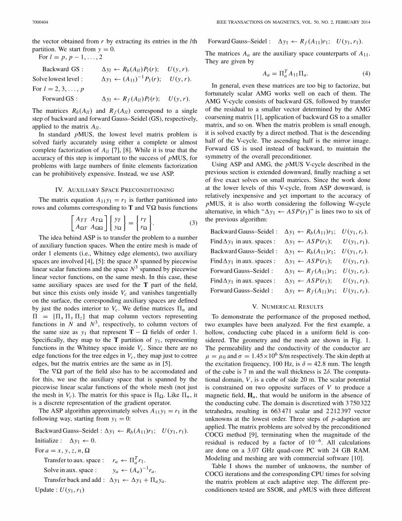
The computational domain is restricted to a cube of 1 medge length with the boundary condition Hnormal = 0 overits surfaces. For the discretization, 1 074 357 tetrahedra areused and the resulting mesh consists of 186 922 nodes and1 267 642 edges. The geometry of the problem (without thesurrounding box) and its discretization in the conductingregion can be observed in Fig. 4(a). Note that the mesh iswell refined on the surface of the conductor regions.

The problem is analyzed p-adaptively in 6 steps. In Table II,the properties of the COCG method for different adaption stepsand different preconditioning algorithms are shown. For theASP method, 2 level AMG is employed for approximatingthe vector nodal systems and the number of unknowns at thelowest level is 36 794. From the experiment, it can be observedthat using ASP for the lowest order correction results in agreatly reduced number of iterations.

More significant than the number of iterations is the CPUtime. The reduction in iterations results in a fewer time-consuming smoothing steps for the higher order blocks ofthe matrix. Fig. 5 compares the time in minutes to solvethe eddy-current problem at each adaption step. Here, weobserve that pMUS[ASP] works very well for the benchmarkproblem and is always faster than SSOR and pMUS[ILU(0)].The cumulative CPU time for all 6 steps using ASP is more

7000404 IEEE TRANSACTIONS ON MAGNETICS, VOL. 50, NO. 2, FEBRUARY 2014

Fig. 4. (a) Mesh discretization for the TEAM 7 benchmark problem.(b) Magnetic field (Re(H)) at the cut plane y = 72 mm.

TABLE II

SOLUTION DETAILS FOR THE TEAM PROBLEM NO. 7

Fig. 5. CPU time versus number of unknowns for different adaption stepsof TEAM 7 eddy-current problem.

than five times less than when using SSOR. For the last fourpoints of the ASP curve, the CPU time grows roughly as N1.1.

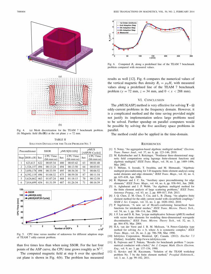
The computed magnetic field at step 6 over the specifiedcut plane is shown in Fig. 4(b). The problem has measured

Fig. 6. Computed Bz along a predefined line of the TEAM 7 benchmarkproblem compared with measured values.

results as well [12]. Fig. 6 compares the numerical values ofthe vertical magnetic flux density Bz = μ0 Hz with measuredvalues along a predefined line of the TEAM 7 benchmarkproblem (y = 72 mm, z = 34 mm, and 0 < x < 288 mm).

VI. CONCLUSION

The pMUS[ASP] method is very effective for solving T−�eddy-current problems in the frequency domain. However, itis a complicated method and the time saving provided mightnot justify its implementation unless large problems needto be solved. Further speedup on parallel computers wouldbe possible by solving the five auxiliary space problems inparallel.

The method could also be applied in the time-domain.

REFERENCES

[1] Y. Notay, “An aggregation-based algebraic multigrid method,” Electron.Trans. Numer. Anal., vol. 37, no. 6, pp. 123–146, 2010.

[2] M. Kaltenbacher and S. Reitzinger, “Nonlinear three-dimensional mag-netic field computations using lagrange finite-element functions andalgebraic multigrid,” IEEE Trans. Magn., vol. 38, no. 3, pp. 1489–1496,May 2002.

[3] T. Mifune, S. Isozaki, T. Iwashita, and M. Shimasaki, “Algebraicmultigrid preconditioning for 3-D magnetic finite-element analyses usingnodal elements and edge elements,” IEEE Trans. Magn., vol. 42, no. 4,pp. 635–638, Apr. 2006.

[4] R. Hiptmair and J. C. Xu, “Auxiliary space preconditioning for edgeelements,” IEEE Trans. Magn., vol. 44, no. 6, pp. 938–941, Jun. 2008.

[5] A. Aghabarati and J. P. Webb, “An algebraic multigrid method forthe finite element analysis of large scattering problems,” IEEE Trans.Antennas Propag., vol. 63, no. 2, pp. 809–817, Feb. 2013.

[6] J. Q. Chen, Z. M. Chen, T. Cui, and L. B. Zhang, “An adaptive finiteelement method for the eddy current model with circuit/field couplings,”SIAM J. Sci. Comput., vol. 32, no. 2, pp. 1020–1042, 2010.

[7] P. Ingelstrom, “A new set of H(curl)-conforming hierarchical basisfunctions for tetrahedral meshes,” IEEE Trans. Microw. Theory Tech.,vol. 54, no. 1, pp. 106–114, Jan. 2006.

[8] J. F. Lee and D. K. Sun, “p-type multiplicative Schwarz (pMUS) methodwith vector finite elements for modeling three-dimensional waveguidediscontinuities,” IEEE Trans. Microw. Theory Tech., vol. 52, no. 3,pp. 864–870, Mar. 2004.

[9] H.A. van der Vorst and J. B. M. Melissen, “A Petrov-Galerkin typemethod for solving Ax = b, where A is symmetric complex,” IEEETrans. Magn., vol. 26, no. 2, pp. 706–708, Mar. 1990.

[10] Infolytica Corporation, Montreal, QC, Canada. (2012). ElecNet 7.3[Online]. Available: http://www.infolytica.com

[11] K. Fujiwara and T. Nakata, “Results for benchmark problem 7 (asym-metrical conductor with a hole),” Int. J. Comput. Math. Electr. Electron.Eng., vol. 9, no. 3, pp. 137–154, 1990.

[12] G. Kovács and M. Kuczmann, “Solution of the TEAM workshopproblem No. 7 by the finite element method,” Przeglad Elektrotech.,vol. 3, no. 3, pp. 99–102, 2011.