
Multilevel Multi-Integration Algorithm for Acoustics
102
Multilevel Multi-Integration Algorithm for Acoustics Isa´ ıas Hern´ andez Ram´ ırez
Transcript of Multilevel Multi-Integration Algorithm for Acoustics
Multilevel Multi-IntegrationAlgorithm for Acoustics
Isaıas Hernandez Ramırez

TABLE OF CONTENTS
1 Introduction 11.1 Sources of sound . . . . . . . . . . . . . . . . . . . . . . . . . . . . . . . . 21.2 Measurement of sound . . . . . . . . . . . . . . . . . . . . . . . . . . . . . 21.3 Problem Classification . . . . . . . . . . . . . . . . . . . . . . . . . . . . . 41.4 Numerical methods . . . . . . . . . . . . . . . . . . . . . . . . . . . . . . . 51.5 Fast matrix multiplication . . . . . . . . . . . . . . . . . . . . . . . . . . . . 71.6 Objective . . . . . . . . . . . . . . . . . . . . . . . . . . . . . . . . . . . . 101.7 Outline . . . . . . . . . . . . . . . . . . . . . . . . . . . . . . . . . . . . . 10
2 Fundamental Solution for Acoustics 132.1 Conservation equations . . . . . . . . . . . . . . . . . . . . . . . . . . . . . 132.2 Acoustic wave equation . . . . . . . . . . . . . . . . . . . . . . . . . . . . . 15
2.2.1 The equation of state . . . . . . . . . . . . . . . . . . . . . . . . . . 152.2.2 The linear wave equation . . . . . . . . . . . . . . . . . . . . . . . . 162.2.3 Boundary conditions . . . . . . . . . . . . . . . . . . . . . . . . . . 17
2.3 The Helmholtz integral representation . . . . . . . . . . . . . . . . . . . . . 192.3.1 The fundamental solution for acoustics . . . . . . . . . . . . . . . . 20
2.4 Evaluation of the Helmholtz Integral Equation . . . . . . . . . . . . . . . . . 21
3 Multi-Level Multi-Integration 233.1 Generic form of the task . . . . . . . . . . . . . . . . . . . . . . . . . . . . 233.2 Multilevel Multi-Integration: Basic Algorithm . . . . . . . . . . . . . . . . . 25
3.2.1 Notation . . . . . . . . . . . . . . . . . . . . . . . . . . . . . . . . 253.2.2 Smooth kernels . . . . . . . . . . . . . . . . . . . . . . . . . . . . . 263.2.3 Asymptotically smooth kernels . . . . . . . . . . . . . . . . . . . . . 29
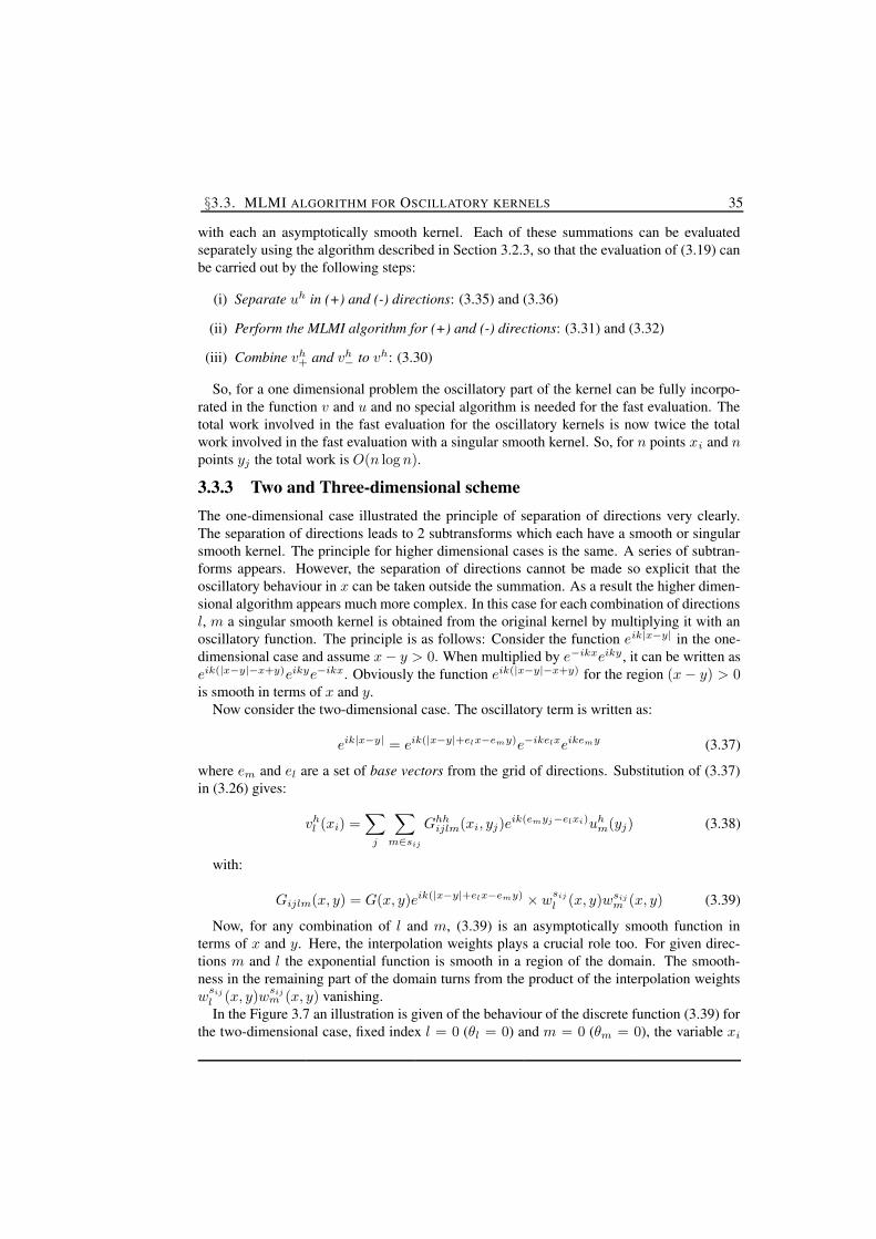
3.3 MLMI algorithm for Oscillatory kernels . . . . . . . . . . . . . . . . . . . . 303.3.1 Separation of directions . . . . . . . . . . . . . . . . . . . . . . . . 323.3.2 One-dimensional scheme . . . . . . . . . . . . . . . . . . . . . . . . 333.3.3 Two and Three-dimensional scheme . . . . . . . . . . . . . . . . . . 353.3.4 Error Control . . . . . . . . . . . . . . . . . . . . . . . . . . . . . . 39
3.4 Estimation of complexity . . . . . . . . . . . . . . . . . . . . . . . . . . . . 41
ii TABLE OF CONTENTS
4 Numerical Results MLMIO 434.1 One dimension (G(x, y) smooth) . . . . . . . . . . . . . . . . . . . . . . . . 43
4.1.1 Discretization . . . . . . . . . . . . . . . . . . . . . . . . . . . . . . 434.1.2 Performance . . . . . . . . . . . . . . . . . . . . . . . . . . . . . . 45
4.2 One dimension (G(x, y) asymptotically smooth) . . . . . . . . . . . . . . . . 504.2.1 Discretization . . . . . . . . . . . . . . . . . . . . . . . . . . . . . . 504.2.2 Performance . . . . . . . . . . . . . . . . . . . . . . . . . . . . . . 52
4.3 Two dimensional problem: G(x, y) explicit oscillatory . . . . . . . . . . . . 564.3.1 Discretization . . . . . . . . . . . . . . . . . . . . . . . . . . . . . . 574.3.2 Performance . . . . . . . . . . . . . . . . . . . . . . . . . . . . . . 58
4.4 Implicit Asymptotically-oscillatory 2D problem . . . . . . . . . . . . . . . . 624.4.1 Discretization . . . . . . . . . . . . . . . . . . . . . . . . . . . . . . 634.4.2 Performance . . . . . . . . . . . . . . . . . . . . . . . . . . . . . . 64
4.5 FFT and MLMIO . . . . . . . . . . . . . . . . . . . . . . . . . . . . . . . . 66
5 Applications 695.1 Helmholtz integral equation . . . . . . . . . . . . . . . . . . . . . . . . . . 695.2 Direct BEM discretization . . . . . . . . . . . . . . . . . . . . . . . . . . . 70
5.2.1 Fast evaluation of the integral transforms using BEM with MLMIO . 725.3 Numerical cases . . . . . . . . . . . . . . . . . . . . . . . . . . . . . . . . . 72
5.3.1 Infinite pulsating cylinder . . . . . . . . . . . . . . . . . . . . . . . 725.3.2 Infinite vibrating wire . . . . . . . . . . . . . . . . . . . . . . . . . 73
6 Conclusions and Recommendations 756.1 Conclusion . . . . . . . . . . . . . . . . . . . . . . . . . . . . . . . . . . . 756.2 Recommandations for further research . . . . . . . . . . . . . . . . . . . . . 76
References 79
A Spatial and angular transfers 85
B Results of the MLMIO algorithm 89B.1 First model problem . . . . . . . . . . . . . . . . . . . . . . . . . . . . . . . 89B.2 Second model problem . . . . . . . . . . . . . . . . . . . . . . . . . . . . . 93B.3 Third model problem . . . . . . . . . . . . . . . . . . . . . . . . . . . . . . 98
1 CH
AP
TE
R
INTRODUCTION
Acoustics is defined as the science of sound, including its production, transmission and ef-fects [51]. Sound can be described as a succession of compressions and rarefactions prop-agating through a medium (solid or fluid) induced by a certain source. Sound is generallycharacterized by its frequency (in Herz) and its intensity (in dB).
Audible sound is the sound that humans are able to perceive such as the voice duringspeech, a car passing on the street, the ringing of (mobile) phones, and music. The frequencyrange of audible sound is between 20 Hz and 20 kHz. Sound with a frequency below 20 Hzis referred to as infrasound. It can not be detected by the human ear. Typical examples ofinfrasound are found in nature; the sound produced by earthquakes or sea waves. Infrasoundcan also be produced by devices used in daily life such woofers, vehicle structures, and fans.Research has indicated that prolonged exposure to infrasound forms a serious health risk[65]. On the other side of the spectrum, ultrasound encompasses all sound with a frequencylarger than the upper limit of the human hearing (20 KHz). In nature, some animals likedogs, dolphins and bats, have an upper limit higher than the human ear and thus can hearultrasound and even use it for navigation and communication. In our society ultrasoundis often used as a diagnostic tool in industry and medicine. For example; ultrasonographyenables visualization of muscles and soft tissues, making it a useful way to scan a humanbody and diagnose specific health problems. Probably the most well-known application ofultrasound is in obstetrics to monitor the foetal development and growth during pregnancy.
The field of acoustics ranges from fundamental physics to engineering, earth sciences, lifesciences, and arts. Pierce [51] gives an overview chart indicating the scope and ramificationsof acoustics. Clearly acoustics affects many aspects of our daily lives.
In engineering in the past decade the attention for acoustics has increased enormously. Themain reason is the need to reduce unwanted sound, or noise. In our society the noise levelto which people are exposed has increased so much that a quiet living and working environ-ment is almost a luxury. The rapidly intensifying use of the urban environment includingthe intertwining of infrastructure, housing, and industry leads to increasingly restrictive de-mands on noise performance of installations, vehicles, and appliances. A low noise level is anessential quality and marketing advantage for products ranging from transport vehicles (air-planes, high-speed trains, trucks, cars) to personal appliances (air conditioners, computers,hair dryers, vacuum cleaners, shavers). For guidance in the design of silent products thereis an urgent need for computational tools to help localize, identify, and accurately predictsources of noise.
2 CHAPTER 1. INTRODUCTION
1.1 Sources of soundSound is the result of a disturbance in a medium. Depending on the source of the disturbance,in acoustical studies in engineering the following classification can be made [74]:
1. Structure induced sound: Sound caused by mechanical vibrations; typical examplesare the vibration of engine casing or the string-body of a piano.
2. Flow induced sound: Sound generated by a disturbed flow such as vortex shedding(von Karman vortex street) or gas jet.
3. Thermally induced sound: Sound caused by local high variations of temperature of thefluid. A typical example is the sound produced by the lightning during storms which isassociated with an electric discharge causing a sudden local expansion of the medium.
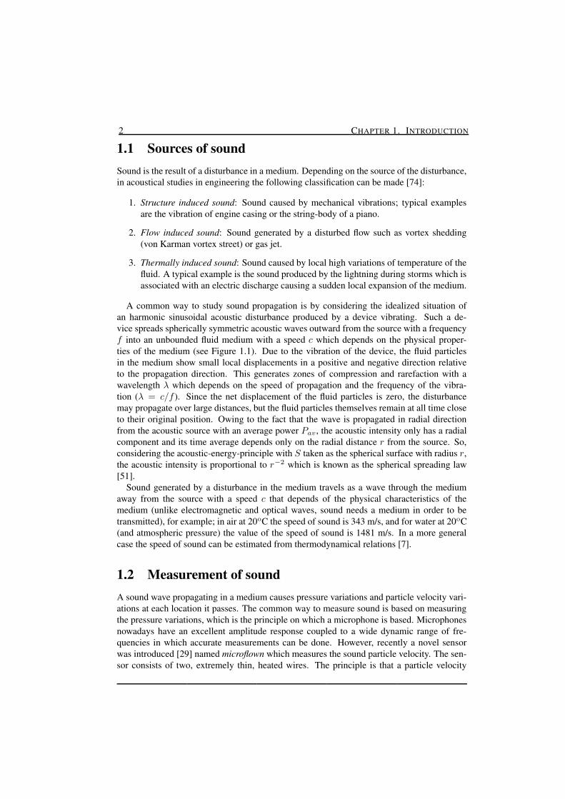
A common way to study sound propagation is by considering the idealized situation ofan harmonic sinusoidal acoustic disturbance produced by a device vibrating. Such a de-vice spreads spherically symmetric acoustic waves outward from the source with a frequencyf into an unbounded fluid medium with a speed c which depends on the physical proper-ties of the medium (see Figure 1.1). Due to the vibration of the device, the fluid particlesin the medium show small local displacements in a positive and negative direction relativeto the propagation direction. This generates zones of compression and rarefaction with awavelength λ which depends on the speed of propagation and the frequency of the vibra-tion (λ = c/f ). Since the net displacement of the fluid particles is zero, the disturbancemay propagate over large distances, but the fluid particles themselves remain at all time closeto their original position. Owing to the fact that the wave is propagated in radial directionfrom the acoustic source with an average power Pav , the acoustic intensity only has a radialcomponent and its time average depends only on the radial distance r from the source. So,considering the acoustic-energy-principle with S taken as the spherical surface with radius r,the acoustic intensity is proportional to r−2 which is known as the spherical spreading law[51].
Sound generated by a disturbance in the medium travels as a wave through the mediumaway from the source with a speed c that depends of the physical characteristics of themedium (unlike electromagnetic and optical waves, sound needs a medium in order to betransmitted), for example; in air at 20oC the speed of sound is 343 m/s, and for water at 20oC(and atmospheric pressure) the value of the speed of sound is 1481 m/s. In a more generalcase the speed of sound can be estimated from thermodynamical relations [7].
1.2 Measurement of soundA sound wave propagating in a medium causes pressure variations and particle velocity vari-ations at each location it passes. The common way to measure sound is based on measuringthe pressure variations, which is the principle on which a microphone is based. Microphonesnowadays have an excellent amplitude response coupled to a wide dynamic range of fre-quencies in which accurate measurements can be done. However, recently a novel sensorwas introduced [29] named microflown which measures the sound particle velocity. The sen-sor consists of two, extremely thin, heated wires. The principle is that a particle velocity
§1.2. MEASUREMENT OF SOUND 3
Compressed
Rarefacted
Sound source
λ
Fluid particle displacement
rp
FIGURE 1.1: Graphical representation of the sound wave propagation in a fluid.The dots represent the fluid particles with small local displacements in the directionindicated by the arrows below which produce a rarefaction and compression whenthe disturbance is propagated out of the source with a wevelength λ.
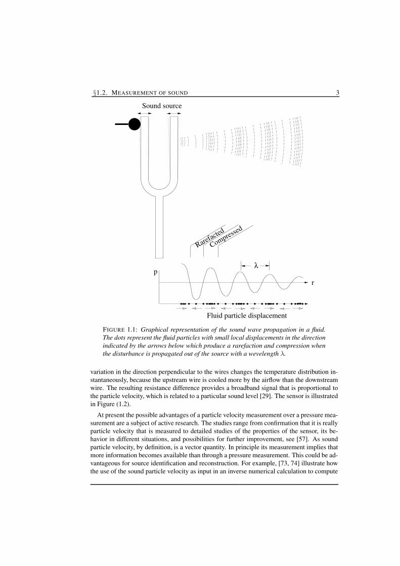
variation in the direction perpendicular to the wires changes the temperature distribution in-stantaneously, because the upstream wire is cooled more by the airflow than the downstreamwire. The resulting resistance difference provides a broadband signal that is proportional tothe particle velocity, which is related to a particular sound level [29]. The sensor is illustratedin Figure (1.2).
At present the possible advantages of a particle velocity measurement over a pressure mea-surement are a subject of active research. The studies range from confirmation that it is reallyparticle velocity that is measured to detailed studies of the properties of the sensor, its be-havior in different situations, and possibilities for further improvement, see [57]. As soundparticle velocity, by definition, is a vector quantity. In principle its measurement implies thatmore information becomes available than through a pressure measurement. This could be ad-vantageous for source identification and reconstruction. For example, [73, 74] illustrate howthe use of the sound particle velocity as input in an inverse numerical calculation to compute
4 CHAPTER 1. INTRODUCTION
FIGURE 1.2: Examples of 3D particle velocity sensor (microflown) combined witha pressure sensor (microphone). (Pictures reproduced with the permission ofµicroflown Technologies)
the source field at the surface generating the sound, leads to a more accurate reconstructionthan the use of the measured pressure as input. Finally, a combination of sound pressure andparticle velocity in a single sensor can give direct information about the acoustic intensity,which again can be useful in source reconstruction [74].
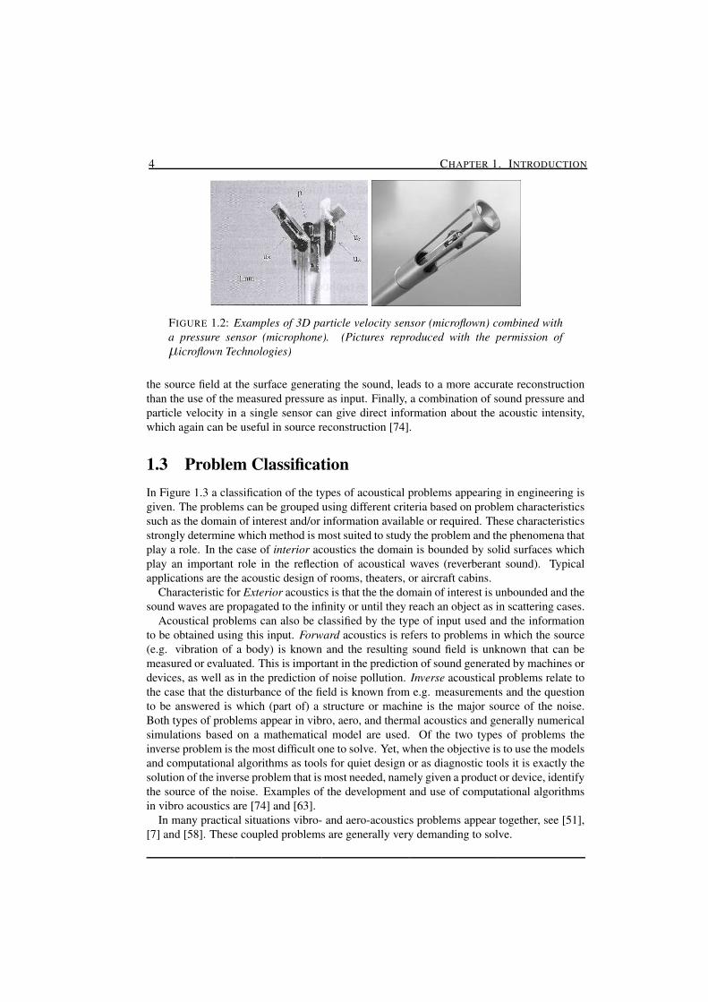
1.3 Problem ClassificationIn Figure 1.3 a classification of the types of acoustical problems appearing in engineering isgiven. The problems can be grouped using different criteria based on problem characteristicssuch as the domain of interest and/or information available or required. These characteristicsstrongly determine which method is most suited to study the problem and the phenomena thatplay a role. In the case of interior acoustics the domain is bounded by solid surfaces whichplay an important role in the reflection of acoustical waves (reverberant sound). Typicalapplications are the acoustic design of rooms, theaters, or aircraft cabins.
Characteristic for Exterior acoustics is that the the domain of interest is unbounded and thesound waves are propagated to the infinity or until they reach an object as in scattering cases.
Acoustical problems can also be classified by the type of input used and the informationto be obtained using this input. Forward acoustics is refers to problems in which the source(e.g. vibration of a body) is known and the resulting sound field is unknown that can bemeasured or evaluated. This is important in the prediction of sound generated by machines ordevices, as well as in the prediction of noise pollution. Inverse acoustical problems relate tothe case that the disturbance of the field is known from e.g. measurements and the questionto be answered is which (part of) a structure or machine is the major source of the noise.Both types of problems appear in vibro, aero, and thermal acoustics and generally numericalsimulations based on a mathematical model are used. Of the two types of problems theinverse problem is the most difficult one to solve. Yet, when the objective is to use the modelsand computational algorithms as tools for quiet design or as diagnostic tools it is exactly thesolution of the inverse problem that is most needed, namely given a product or device, identifythe source of the noise. Examples of the development and use of computational algorithmsin vibro acoustics are [74] and [63].
In many practical situations vibro- and aero-acoustics problems appear together, see [51],[7] and [58]. These coupled problems are generally very demanding to solve.
§1.4. NUMERICAL METHODS 5
Inverse acoustics(source unknown)
AcousticSensors
Vibro−Acoustics Aero−Acoustics Thermo−Acoustics
Coupled problems
SensorsAcoustic
Γ
Ω
Exterior Acoustics
Ω
Γ
Γ
Interior acoustics
AcousticalProblems
Forward acoustics(consequence unknown)
FIGURE 1.3: A possible clasification of acoustical problems found in engineeringapplications.
1.4 Numerical methods
In this thesis we restrict ourselves to vibro-acoustic problems and it is assumed that a model isused based on the Helmholtz equation with the associated boundary conditions, see chapter2. Even then, only in much simplified cases the problem can be solved analytically. Ingeneral a numerical approach is necessary. During past decades different approaches havebeen proposed (see e.g. [22], [30], [41], [42], [46], [51] and [76]). Two approaches havebecome very common:
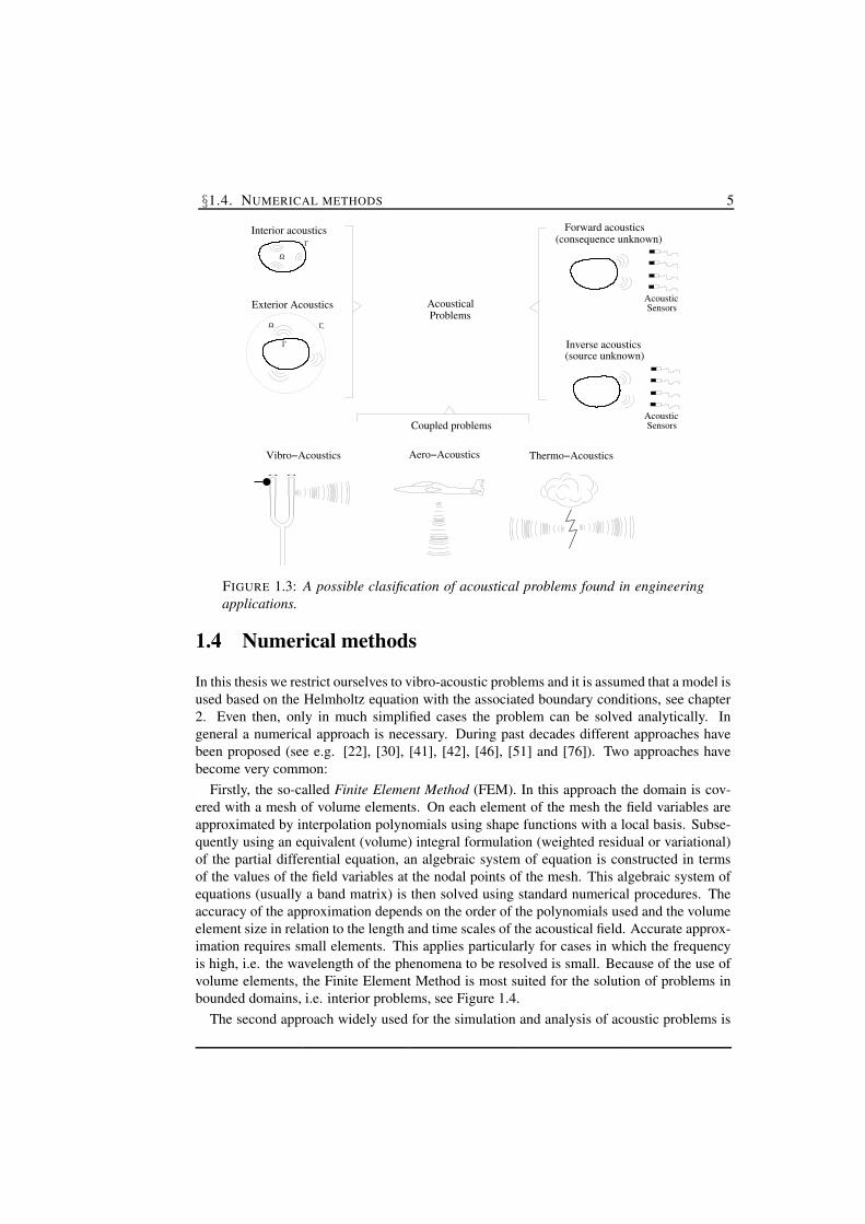
Firstly, the so-called Finite Element Method (FEM). In this approach the domain is cov-ered with a mesh of volume elements. On each element of the mesh the field variables areapproximated by interpolation polynomials using shape functions with a local basis. Subse-quently using an equivalent (volume) integral formulation (weighted residual or variational)of the partial differential equation, an algebraic system of equation is constructed in termsof the values of the field variables at the nodal points of the mesh. This algebraic system ofequations (usually a band matrix) is then solved using standard numerical procedures. Theaccuracy of the approximation depends on the order of the polynomials used and the volumeelement size in relation to the length and time scales of the acoustical field. Accurate approx-imation requires small elements. This applies particularly for cases in which the frequencyis high, i.e. the wavelength of the phenomena to be resolved is small. Because of the use ofvolume elements, the Finite Element Method is most suited for the solution of problems inbounded domains, i.e. interior problems, see Figure 1.4.
The second approach widely used for the simulation and analysis of acoustic problems is

6 CHAPTER 1. INTRODUCTION
ExteriorDomain
BoundaryDiscretization
Artificialfar-field
boundary
InteriorDomain
FIGURE 1.4: Schematic representation of the discretization for a volumen andboundary domain.
the Boundary Element Method (BEM), e.g. [22], [48], [43], and [44]). The method is basedon the (direct or indirect) boundary integral formulation of the problem. Using elementarysolutions of the governing partial differential equation and the boundary conditions the prob-lem of solving the field variables in the domain is replaced by the solving an integral equationfor the strength of the distribution of elementary solutions on the boundary of the domain,e.g. see [22]. Once this distribution is known, using the form of the elementary solution, thevalue of the field variables in any point in the domain can be obtained from an integral overthe distribution on the boundary. Since the elementary solutions satisfy the boundary condi-tion of infinity the boundary element method is very well suited for exterior problems. In thenumerical approach, similar to the finite element method, in the boundary element methodthe problem of solving the continuous integral equation is replaced by a discrete formulationleading to an algebraic system that can be solved by computer. The way this is done is es-sentially the same as in the finite element method, i.e. the boundary is covered with a grid,see Figure 1.4. On each of the elements of the grid the boundary variable is approximated byan interpolation polynomial using shape functions with local support and using a variationalor collocation formulation an algebraic system of equations is obtained that can be solved bystandard numerical routines.
The Boundary Element Method is very well suited for problems on a large domain, i.e.
§1.5. FAST MATRIX MULTIPLICATION 7
radiated sound problems. Instead of the need to cover the full domain with a mesh, onlythe boundary of the domain needs to be covered with a mesh. However, it also has somedisadvantages. One difficulty is that it requires approximation of an integral equation witha singular kernel (Green’s function). The second is that the resulting system of algebraicequations is generally a fully populated complex system which is very expensive to solvenumerically. Typically the computing time will be O(n3), with n the number of unknowns(boundary elements). Finally, on top of that, to obtain the value of a field variable at pointof the exterior domain a (discrete) integral transform has to be evaluated which requires asummation over all the boundary elements and thus O(n) operations for each point at whichthe field is to be determined. This may lead to excessive computing times for large n or incase the field is to be computed at a large number of points. Often in practical problemsindeed large n is required to have a sufficiently accurate approximation, particularly so forhigh frequencies.
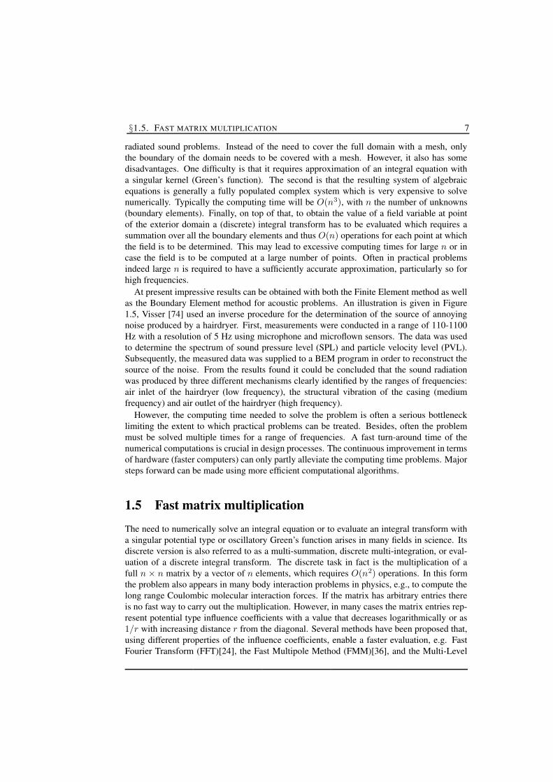
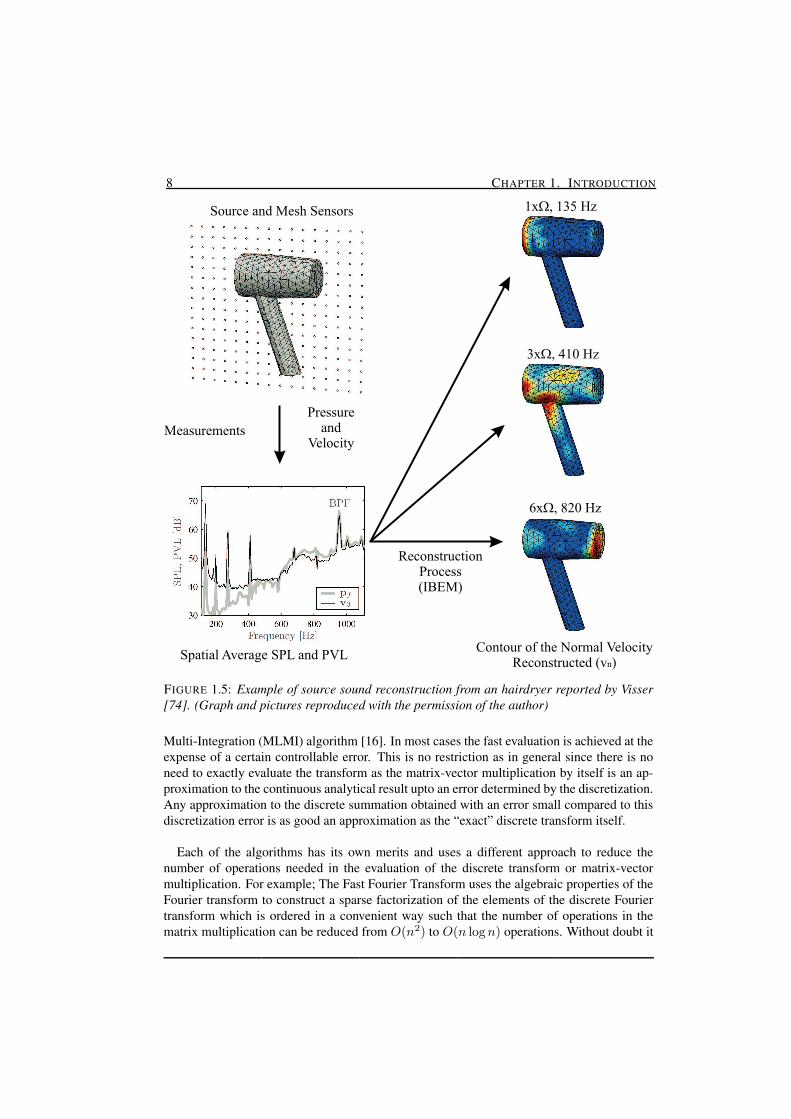
At present impressive results can be obtained with both the Finite Element method as wellas the Boundary Element method for acoustic problems. An illustration is given in Figure1.5, Visser [74] used an inverse procedure for the determination of the source of annoyingnoise produced by a hairdryer. First, measurements were conducted in a range of 110-1100Hz with a resolution of 5 Hz using microphone and microflown sensors. The data was usedto determine the spectrum of sound pressure level (SPL) and particle velocity level (PVL).Subsequently, the measured data was supplied to a BEM program in order to reconstruct thesource of the noise. From the results found it could be concluded that the sound radiationwas produced by three different mechanisms clearly identified by the ranges of frequencies:air inlet of the hairdryer (low frequency), the structural vibration of the casing (mediumfrequency) and air outlet of the hairdryer (high frequency).
However, the computing time needed to solve the problem is often a serious bottlenecklimiting the extent to which practical problems can be treated. Besides, often the problemmust be solved multiple times for a range of frequencies. A fast turn-around time of thenumerical computations is crucial in design processes. The continuous improvement in termsof hardware (faster computers) can only partly alleviate the computing time problems. Majorsteps forward can be made using more efficient computational algorithms.
1.5 Fast matrix multiplication
The need to numerically solve an integral equation or to evaluate an integral transform witha singular potential type or oscillatory Green’s function arises in many fields in science. Itsdiscrete version is also referred to as a multi-summation, discrete multi-integration, or eval-uation of a discrete integral transform. The discrete task in fact is the multiplication of afull n × n matrix by a vector of n elements, which requires O(n2) operations. In this formthe problem also appears in many body interaction problems in physics, e.g., to compute thelong range Coulombic molecular interaction forces. If the matrix has arbitrary entries thereis no fast way to carry out the multiplication. However, in many cases the matrix entries rep-resent potential type influence coefficients with a value that decreases logarithmically or as1/r with increasing distance r from the diagonal. Several methods have been proposed that,using different properties of the influence coefficients, enable a faster evaluation, e.g. FastFourier Transform (FFT)[24], the Fast Multipole Method (FMM)[36], and the Multi-Level
8 CHAPTER 1. INTRODUCTION
Measurements
Pressureand
Velocity
Spatial Average SPL and PVLContour of the Normal Velocity
Reconstructed (v )n
1x , 135 HzW
3x , 410 HzW
6x , 820 HzW
Source and Mesh Sensors
ReconstructionProcess(IBEM)
FIGURE 1.5: Example of source sound reconstruction from an hairdryer reported by Visser[74]. (Graph and pictures reproduced with the permission of the author)
Multi-Integration (MLMI) algorithm [16]. In most cases the fast evaluation is achieved at theexpense of a certain controllable error. This is no restriction as in general since there is noneed to exactly evaluate the transform as the matrix-vector multiplication by itself is an ap-proximation to the continuous analytical result upto an error determined by the discretization.Any approximation to the discrete summation obtained with an error small compared to thisdiscretization error is as good an approximation as the “exact” discrete transform itself.
Each of the algorithms has its own merits and uses a different approach to reduce thenumber of operations needed in the evaluation of the discrete transform or matrix-vectormultiplication. For example; The Fast Fourier Transform uses the algebraic properties of theFourier transform to construct a sparse factorization of the elements of the discrete Fouriertransform which is ordered in a convenient way such that the number of operations in thematrix multiplication can be reduced from O(n2) to O(n log n) operations. Without doubt it
§1.5. FAST MATRIX MULTIPLICATION 9
is one of the simplest and most efficient algorithms. However, its application is also limitedto uniform non-curvilinear (Cartesian) grids.
The Fast Multipole Method uses a tree type of scheme and a set of polynomial expansionsto represent the far-field and intermediate influence of the elements or particles. The centralstrategy used is that of clustering at various spatial lenghts and the compution of the inter-action with other clusters which are sufficiently far away by means of multipole expansions.For elements in the near field, this assumption is no longer valid, so that, a direct computationis performed only in a small region. Using the Fast Multipole Method at the expense of anerror controlled by the accuracy of the expansions and the size of the near field the computingtime needed can be reduced from O(n2) to O(n log n) operations.
Multilevel Multi-Integration was introduced by Brandt and Lubrecht [16]. In this algorithmthe smoothness properties of the Green’s functions are exploited, this also determine the prop-erties of the dense matrix. The key is that in regions where the (discrete) Green’s function issmooth it can be represented accurately by interpolation from a reduced data set of the valuesof the Green’s functions at a limited number of points. As a result the matrix-vector evalua-tion can be replaced by an equivalent matrix-vector multiplication involving the reduced dataset and some transfer operators from the original to the reduced data set and back from thereduced problem to the full problem. For smooth Green’s functions it allows a computingtime reduction from O(n2) to O(n). For singular smooth Green’s functions computing timeis reduced from O(n2) to O(n log n). An advantage of Multilevel Multi-Integration is that inits basic form it is straightforward to implement. Besides, it can be applied to any dense ma-trix vector multiplication without the need to make any assumption about its behavior. Alsoit can be applied to curved surfaces and extended to non-uniform grids. Besides, any errormade in the fast evaluation can be corrected employing an a posteriori correction.
These methods have been applied successfully for particle interactions and for integraltransforms related to problems governed by the Laplace equations for which Green’s func-tions are asymptotically smooth (e.g. log |r|, 1/r). Computing time reductions have beenreported up to orders of magnitude, see [36], [16], [50], [60], [70] and [13]. As a result of thereduced computing times larger and more practical problems could be considered leading tosignificant advances in the fields.
Numerical studies of boundary integral problems based on the Helmholtz equation canalso significantly benefit from faster and more efficient algorithms. The implementation ofmore efficient techniques for such problems, for which the Green’s function appearing in thetransform is oscillatory, has indeed begun. In [50] has used the panel method for the dis-cretization of the body surfaces and developed an approach based on the idea to represent thelong-range part of the potential by point charges located on an uniform grid, which then al-lows fast evaluation using FFT, whereas the short-range interaction is still computed directly.The approach consists of two steps. First a transform is carried out of the boundary variablefrom the non-uniform curved boundary to a uniform non-curved grid. The second step is FFTto compute the integral transform represented on the grid. The final step is to interpolate thecomputed values of the discrete integral transform on the grid back to the non-uniform curvedboundary followed by a local correction. Compared to simple direct summation to obtain theresult large computing time reductions have been achieved.
The fast multipole method developed by Rokhlin and co-workers [60] has been appliedto a variety of problems, including cases with oscillatory kernels [23], [27], [43] and [66].Recently Drave [28] has given a set of guidelines for the numerical implementation of the
10 CHAPTER 1. INTRODUCTION
multipole method based on a physical interpretation of the method, which can be seen as asuperposition of plane waves. In the method it is asssumed that a simple radiating source pointR(P ) is located at the origin, and an observation point P is located in the field. When P is farenough from the origin R can locally be approximated by a single plane wave, with directionof propagation P/|P |. As P gets closer to the origin R(P ) will no longer be approximatedwell by a single plane wave but rather by a superposition of plane waves. Depending on theaccuracy desired, the number of terms in the expansion needs to be increased, and the methodcan evaluate problems in O(n3/2), O(n4/3) or even O(n log n) operations.
The multilevel multi-integration method has not extensively been used for Helmholtz re-lated boundary integral problems yet. Recently Grigoriev and Dargush [37] presented resultsfor a two-dimensional boundary element method program based on the direct formulation.For the fast evaluation of the integral transforms related with the distributions on the bound-ary surface (contour in 2D) they used the standard multilevel multi-integration algorithm of[16]. Moreover, they implemented a conjugate gradient scheme for solving the discretizedintegral equation. The results confirmed the expectation that a significant speed up was attain-able using the multilevel algorithm. However, their algorithm was only limited to moderatewave numbers. As mentioned above the Multilevel Multi-Integration algorithm exploits thesmoothness properties of the Green’s function. For high wavenumbers the oscillatory Green’sfunction appearing in acoustic problems is obviously not smooth and when using the stan-dard MLMI algorithm the attainable improvement in efficiency will strongly depend on thefrequency. The generalization of the Multilevel Multi-Integration algorithm to the case ofoscillatory kernels was already described in 1991 by Brandt [14]. It is claimed that indepen-dent of the frequency the computational effort of the discrete evaluation can be reduced fromO(n2) to O(npd log n) operations with p the order of polynomial and d the dimension of theproblem (e.g. d = 3 for 3D). However, as far as known to the author no evidence that thealgorithm really works has been published so far 2D.
1.6 ObjectiveThe objective of the research presented in this thesis is the development and implementa-tion of a Multilevel Multi-Integration algorithm along the lines suggested by Brandt in [14]for the fast evaluation of discrete integral transforms with oscillatory kernels as they appearin Boundary Element formulations of acoustic radiation problems. Eventually the algorithmshould be combined with the Boundary Element Method proposed by [74] for source identifi-cation to alleviate the computing time problems and enable larger and more realistic problemsto be solved. The project has been part of a larger project with the aim to develop efficientnumerical and experimental tools for the determination of radiated noise and acoustic sourceidentification.
1.7 OutlineIn the chapter 2 a brief overview of relevant theory is given. This includes the derivation ofthe Helmholtz equation. It is tranformed in its integral version using the Green theorem. Themore common boundary conditions are described and the fundamental solutions for acous-tical problems are presented. Furthermore the chapter briefly describes the type of integral

§1.7. OUTLINE 11
transforms to be evaluated.In chapter 3 the Multilevel Multi-Integration algorithm is explained taking a generic form
of the integral transform as model problem. First the basic algorithm for smooth and asymp-totically smooth algorithms is described. Subsequently the generalization of the algorithm tothe case of oscillatory kernels is outlined.
In chapter 4 numerical results are presented for a number of representative one and twodimensional problems. It is illustrated that the generalized Multilevel Multi-Integration algo-rithm as proposed by Brandt in [14] really works and for large n yields substantial computingtime reductions. For reference a comparison with results obtained using Fast Fourier Trans-form is given. Further improvement is even possible by further optimization
In chapter 5 results of the implementation of the algorithm for some acoustic problemsanalysed with a Boundary Element Method are given.
The thesis is concluded with concluding remarks and recommendations for further re-search.

12 CHAPTER 1. INTRODUCTION
2 CH
AP
TE
RFUNDAMENTAL SOLUTION FOR
ACOUSTICS
In this chapter a brief description is given of the theory related to acoustics. It starts withthe linearization of the conservation equations of mass, momentum and energy. A generalrepresentation of the wave equation for acoustics is shown. Further, the more fundamentalsolutions (Green’s function) of the wave equation is described and the integral formulationsuitable for acoustic radiation problems is given. Attention is given to the treatment of thefundamental solutions for infinite domains and the conditions which have to be satisfied.Finally, the complications arising from the need to evaluate the resulting integrals in practicalapplications are discussed.
2.1 Conservation equations
In the continuum theory of fluids, a fluid (liquid or gas) is regarded as a continuous rela-tively dense distribution of particles, with uniform properties. Conservation laws are derivedwhich describe the changes in space and time of the field variables: velocity, pressure, den-sity, temperature, etc., of the fluid. The physical principles of mass, momentum and energyconservation are the starting point in the derivation of equations that describe acoustic phe-nomena. Their derivation can be found in standard text books, see [4] and [6]. A specificdifferential formulation of the basic conservation laws is:
• Mass conservation.Dρ
Dt+ ρ∇ · v = 0, (2.1)
• Momentum conservation, for constant µ and λ and neglecting any external force filed.
ρDv
Dt+ ∇p = (λ + 2µ)∇(∇ · v) − µ∇× (∇× v), (2.2)
• Energy conservation, neglecting volumetric heat sources (adiabatic) and employingFourier’s low of heat conduction (q = −k∇T .
ρDe
Dt+ p∇ · v = Φvisc + κ∇2T, (2.3)
14 CHAPTER 2. FUNDAMENTAL SOLUTION FOR ACOUSTICS
where DDt represents the material derivative∗, and the field variables of the fluid the velocity
(v), density (ρ), pressure (p), temperature (T ) and internal energy (e). The term Φvisc isdefined as the three-dimensional viscous energy dissipation function (a nonlinear quantity) †.Alternatively the energy can be expressed as:
ρDs
Dt=
1
T
[
Φvisc + κ∇2T]
(2.4)
The equations of conservation of mass, momentum and energy and the used relations forthe viscous stress terms and the heat flux are not a completely closed system of equations.Additional relationships are required. These additional relations are the equations of statebetween thermodynamic variables. They follow from the law of thermodynamics an thethermodynamics state principle: if the chemical composition of a fluid is fixed then the localthermodynamic state is fixed completely by two independent variables. So one could choosethe density ρ and the specific entropy.
T = T (s, ρ) (2.5)
p = p(s, ρ) (2.6)
Depending of the specific application the equations, (2.1)-(2.3), and (2.6), can be simplified[7]:
1. Incompressible flow. DρDt = 0. In this case the equation of continuity reduces to ∇·v =
0, which means that also several terms in the other equations vanish. (Incompressibleflows are of interest in fields as hydraulics, civil engineering, low-speed aerodynamics,etc.)
2. Time-independent or steady state flow. Here a considerable simplification occurs be-cause the time derivative terms vanish. (Steady flows are of interest in aerodynamics,hydraulics, pipe flow, etc.)
3. Lossless flow. When effects of viscosity and heat conduction can be neglected (λ,µ, κ = 0), also many terms vanish. Important fluid flow problems, including soundpropagation, can be approximated as lossless flow.
4. Small-perturbation flow. Linearization of the equations is helpful to deal with manykind of problems. Most sound waves are considered as small disturbances onto a mainflow field.
As has been mentioned under 3) and 4), lossless and small perturbation flow are the mainassumptions applied in the study of acoustics. Of course, effects of viscosity and heat conduc-tion on acoustic waves can be taken into account for small perturbations in the conservationlaws. However, this is beyond the scope of this thesis.
∗The material derivative operator is defined by: DDt
= ∂∂t
+ v · ∇†Φvisc has been defined by some authors in tensor form as: Φvisc = 2µdijdji + λdkkdii, where the rate
of deformation is dij = 12(vi,j + vj,i), µ is the dynamic viscosity of the fluid, and λ the viscosity dilatation
coefficient.
§2.2. ACOUSTIC WAVE EQUATION 15
2.2 Acoustic wave equationAcoustic disturbances can often be regarded as small-amplitude perturbations to an ambientstate [51]. In that case the perturbations can be solved from a linearization of the conser-vation equations. The justification is that most acoustic disturbances are so small that thenonlinear terms in the conservation equations are not important [7]. Nonetheless, the exactform of the resulting wave equation depends on the assumptions made about the nature ofthe wave motion and the medium. Blackstock [7] and Pierce [51] give a linearization forthe case a viscous and thermally conducting fluid is considered. Here the simplest and mostcommon acoustic linearization is dicussed which applies for problems for which the mediummay be characterized as inviscid and thermally nonconducting. In that case the continuity,momentum and energy equations can be written as:
∂ρ
∂t+ ∇ · (ρv) = 0 (2.7)
ρ
[
Dv
Dt
]
+ ∇p = 0 (2.8)
ρDs
Dt= 0 (2.9)
where (2.8) is known as Euler’s equation of inviscid motion. Note that the energy equationindicates that for adiabatic flow of a inviscid non-heat-conducting fluid the entropy remainsconstant when moving with a fluid element.
2.2.1 The equation of stateFor any fluid the equation of state relates physical quantities describing the thermodynamicbehaviour of the fluid. For an adiabatic and reversible process (nearly isentropic) it is prefer-able to determine experimentally the relationship between pressure and density fluctuations.The relationship can be represented by a Taylor series expansion
p − p0 =
(
∂p
∂ρ
)
0
(ρ − ρ0) +1
2
(
∂2p
∂ρ2
)
0
(ρ − ρ0)2 + ... (2.10)
with the partial derivatives determined for isentropic compression and expansion of the fluidabout its equilibrium density. If the fluctuations are small (assumption for linear acoustics)only the lowest order terms in (ρ − ρ0) need be retained, which gives a linear relationshipbetween the pressure fluctuations and the change in the density.
p − p0 ≈ β(ρ − ρ0)
ρ0(2.11)
where β = ρ0(∂p∂ρ )s is the so-called adiabatic bulk modulus‡ and (ρ − ρ0)/ρ0 is known as
the condensation term [41].
‡The adiabatic bulk modulus is defined as the change of the pressure as a function of the volume at constantentropy
“
β = ρ“
∂p∂ρ
”
s
”
, and it has a direct relation with the speed of sound c.
16 CHAPTER 2. FUNDAMENTAL SOLUTION FOR ACOUSTICS
2.2.2 The linear wave equationA fluid is considered at rest when the field variables; pressure (p = p0), density (ρ = ρ0)and velocity (v = 0) are absent of any perturbation. Furthermore, a medium is consideredhomogeneous when all ambient quantities are independent of the position, and when themedium is quiescent, they are independent of the time. In many cases, the idealization ofa homogeneous quiesent medium is satisfactory for the description of acoustic phenomena[51].
The field variables of a fluid at rest satisfy the fluid dynamics equations (or conservationlaws). However, when the fluid is disturbed for an acoustical perturbation, these variablescan be represented by,
p(x, t) = p0 + p′(x, t), ρ(x, t) = ρ0 + ρ′(x, t), v(x, t) = v′(x, t), (2.12)
where p′, ρ′ and v′, all a function of space and time represent the acoustic perturbation of thefluid.
The mass conservation equation (2.7), the Euler equation (2.8), and the state equation withconstant entropy (p = p(ρ, s) and s = s0) can be written in terms of the acoustic disturbances.Here v = v′; p0 and ρ0 are constants related by p0 = p(ρ0, s0).
∂
∂t(ρ0 + ρ′) + ∇ · [(ρ0 + ρ′)v′] = 0 (2.13)
(ρ0 + ρ′)
(
∂
∂t+ v′ · ∇
)
v′ = −∇(p0 + p′) (2.14)
p0 + p′ = p(ρ0 + ρ′, s0) (2.15)
The terms in the equations (2.13)-(2.15) can be grouped into zero, first, and higher-orderterms. In Equation (2.15), the grouping resulting from a Taylor-series expansion for small ρ′
is,
p′ =
(
∂p
∂ρ
)
ρ0,s0
ρ′ +1
2
(
∂2p
∂ρ2
)
ρ0,s0
(ρ′)2 + ... (2.16)
Neglecting all terms of second order and higher results in the equations of linear acoustics inthe case of a quiesent medium:
∂ρ′
∂t+ ρ0∇ · v′ = 0 (2.17)
ρ0∂v′
∂t= −∇p′ (2.18)
p′ = c2ρ′, with c2 =
(
∂p
∂ρ
)
s0
(2.19)
Thermodynamic considerations require that c2 always be positive. Here c is defined as thespeed of sound in the medium. Of course, in general c can be a function of position and

§2.2. ACOUSTIC WAVE EQUATION 17
of time. This variation can depend on the specific properties of the fluid (e.g. when thethermodynamic properties are not constant in the domain, the speed of sound will also notbe constant). When equations (2.17) and (2.18) are combined to eliminate the dependency ofthe velocity from (2.17), the resulting equation is:
∂2ρ′
∂t2−∇2p′ = 0 (2.20)
Substitution of (2.19) in (2.20) leads to the wave equation for the acoustic pressure:
∇2p′ − 1
c2
∂2p′
∂t2= 0 (2.21)
This is the most fundamental equation in acoustics. It describes the properties of a soundfield in space and time.
From (2.17)-(2.19) we can also derive that p′(x, t) and v′(x, t) also satisfy the wave equa-tion.
If the solution of (2.21) is assumed to be time harmonic; e.g.,
p′(x, t) = p(x)eıωt (2.22)
with ω the angular frequency (ω = 2πf ) and p the amplitude, equation (2.21) can be trans-formed from the time domain to the frequency domain. The resulting equation is known asthe Helmholtz partial differential equation.
∇2p + k2p = 0 (2.23)
where k = ω/c, is known as the wave number. Assuming that v′ and ρ′ are also timeharmonic, with the same frequency, also results in a Helmholtz equation for v(x) and ρ(x).Furthermore, it follows directly from (2.18) that
v(x) =i
ρ0ω∇p (2.24)
and from (2.19): ρ(x) = 1c2 p(x). In the successive we drop the (ˆ ) on the variables.
2.2.3 Boundary conditions
To determine the pressure field solving Helmholtz’s equation (2.23) for domain ΩV (seeFigure 2.1), boundary conditions ΓS must be specified at each position on the boundaryS = ∂ΩV of the domain. Depending on the type of fluid domain (bounded or unbounded),the following boundary conditions may occur.Interior acoustic problem. The fluid domain is bounded by the surface S, and boundaryconditions of the following three types may occur on the closed boundary surface ΓS =Γp ∪ Γvn
∪ ΓZ :
• Dirichlet condition (imposed pressure)
p = pS on Γp (2.25)
18 CHAPTER 2. FUNDAMENTAL SOLUTION FOR ACOUSTICS
V
x
y
ΩΓp
Γp
Γvn
z
b) Exterior acousticsa) Interior acoustics
ZΓn
n
n
Γ
ΩV ZΓ
Γv
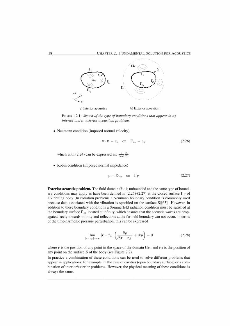
FIGURE 2.1: Sketch of the type of boundary conditions that appear in a)interior and b) exterior acoustical problems.
• Neumann condition (imposed normal velocity)
v · n = vn on Γvn= vn (2.26)
which with (2.24) can be expressed as: ıρ0ω
∂p∂n
• Robin condition (imposed normal impedance)
p = Zvn on ΓZ (2.27)
Exterior acoustic problem. The fluid domain ΩV is unbounded and the same type of bound-ary conditions may apply as have been defined in (2.25)-(2.27) at the closed surface ΓS ofa vibrating body (In radiation problems a Neumann boundary condition is commonly usedbecause data associated with the vibration is specified on the surface S)[63]. However, inaddition to these boundary conditions a Sommerfeld radiation condition must be satisfied atthe boundary surface Γ∞ located at infinity, which ensures that the acoustic waves are prop-agated freely towards infinity and reflections at the far field boundary can not occur. In termsof the time-harmonic pressure perturbation, this can be expressed
lim|r−rS |→∞
|r − rS |(
∂p
∂|r − rS |+ ıkp
)
= 0 (2.28)
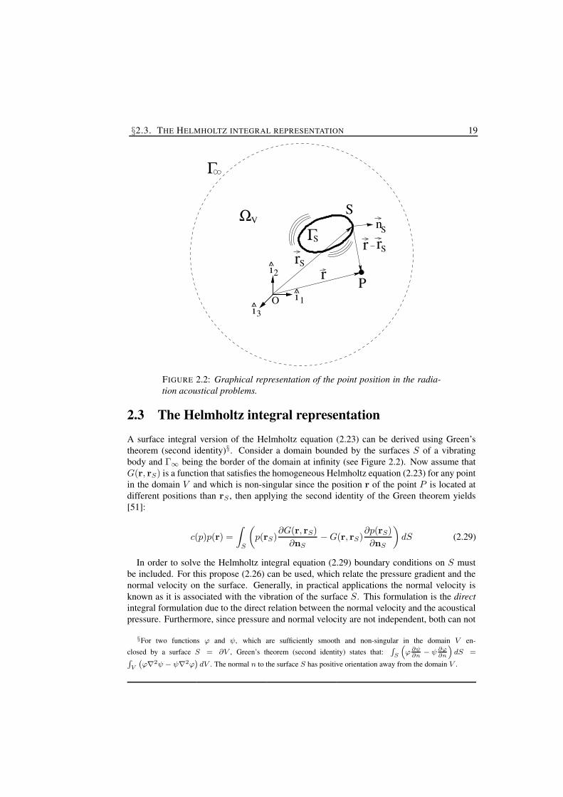
where r is the position of any point in the space of the domain ΩV , and rS is the position ofany point on the surface S of the body (see Figure 2.2).In practice a combination of these conditions can be used to solve different problems thatappear in applications; for example, in the case of cavities (open boundary surface) or a com-bination of interior/exterior problems. However, the physical meaning of these conditions isalways the same.
§2.3. THE HELMHOLTZ INTEGRAL REPRESENTATION 19
rS
r
S
P
r
V
i
Ω
Γ
Sr
^O
nSΓS
2
1i3
i
FIGURE 2.2: Graphical representation of the point position in the radia-tion acoustical problems.
2.3 The Helmholtz integral representation
A surface integral version of the Helmholtz equation (2.23) can be derived using Green’stheorem (second identity)§. Consider a domain bounded by the surfaces S of a vibratingbody and Γ∞ being the border of the domain at infinity (see Figure 2.2). Now assume thatG(r, rS) is a function that satisfies the homogeneous Helmholtz equation (2.23) for any pointin the domain V and which is non-singular since the position r of the point P is located atdifferent positions than rS , then applying the second identity of the Green theorem yields[51]:
c(p)p(r) =
∫
S
(
p(rS)∂G(r, rS)
∂nS− G(r, rS)
∂p(rS)
∂nS
)
dS (2.29)
In order to solve the Helmholtz integral equation (2.29) boundary conditions on S mustbe included. For this propose (2.26) can be used, which relate the pressure gradient and thenormal velocity on the surface. Generally, in practical applications the normal velocity isknown as it is associated with the vibration of the surface S. This formulation is the directintegral formulation due to the direct relation between the normal velocity and the acousticalpressure. Furthermore, since pressure and normal velocity are not independent, both can not
§For two functions ϕ and ψ, which are sufficiently smooth and non-singular in the domain V en-closed by a surface S = ∂V , Green’s theorem (second identity) states that:
R
S
“
ϕ∂ψ∂n
− ψ∂ϕ∂n
”
dS =R
V
`
ϕ∇2ψ − ψ∇2ϕ´
dV . The normal n to the surface S has positive orientation away from the domain V .
20 CHAPTER 2. FUNDAMENTAL SOLUTION FOR ACOUSTICS
be prescribed on the surface S; this means that a prescribed normal velocity on the surface Scauses a certain pressure on S, and vice versa [63].
The contribution from the far field boundary (Γ∞) of the acoustic domain has been re-moved analytically by invoking the Sommerfeld radiation condition (2.28) which is automat-ically satisfied in the sense that the surface normal vector always points out of the domain. Inthis way, the characteristic impedance (p/vn = −ρc, when |r− rs| → ∞) is negative, whichensures that no reflecting waves occur. Equation (2.29) can be written as:
c(p)p(r) =
∫
S
(
p(rS)∂G(r, rS)
∂nS+ ıρ0ωG(r, rS)vnS
)
dS (2.30)
In (2.29) and (2.30) c(p) is known as the geometry coefficient, which can be represented bythe integral form [74]:
• When the normal vector on ΓS is uniquely defined.
c(p) =
1 for x ∈ ΩV12 for x ∈ ΓS
0 for x /∈ ΩV
(2.31)
• When the normal vector on ΓS is not uniquely defined: e.g at corners and edges.
– Interior problems:
c(p) =1
4π
∫
∂
∂n
1
rdS (2.32)
– Exterior problems:
c(p) = 1 +1
4π
∫
∂
∂n
1
rdS (2.33)
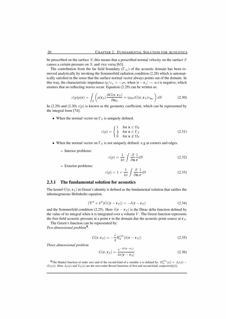
2.3.1 The fundamental solution for acousticsThe kernel G(r, rS) in Green’s identity is defined as the fundamental solution that satifies theinhomogeneous Helmholtz equation.
(∇2 + k2)G(|r− rS |) = −δ(r − rS) (2.34)
and the Sommerfeld condition (2.25). Here δ(r − rS) is the Dirac delta function defined bythe value of its integral when it is integrated over a volume V . The Green function representsthe free-field acoustic pressure at a point r in the domain due the acoustic point source at rS .
The Green’s function can be represented by:Two-dimensional problem¶.
G(r, rS) = − i
4H
(2)0 (k|r − rS|) (2.35)
Three-dimensional problem
G(r, rS) =e−ık|r−rS |
4π|r − rS|(2.36)
¶The Hankel function of order zero and of the second kind of a variable φ is defined by: H (2)0 (φ) = J0(φ) −
ıY0(φ). Here J0(φ) and Y0(φ) are the zero-order Bessel functions of first and second kind, respectively[1].

§2.4. EVALUATION OF THE HELMHOLTZ INTEGRAL EQUATION 21
Note that the Green’s function is a complex valued function, which becomes singular whenthe distance |r − rS| between the field position and the source position becomes zero.
2.4 Evaluation of the Helmholtz Integral EquationInlcuding the Neumann boundary conditions in the Equation (2.30) and reordering in termsof known and unknown quantities. The integral equation that represents the pressure on thesurface of an vibrating body is given by:
c(p)p(r)−∫
S
p(rS)∂G(r, rS)
∂nSdS = ıρ0ω
∫
S
G(r, rS)vnSdS (2.37)
The evaluation of the direct Helmholtz integral equation (2.37) is generally performed intwo steps [22][51][74]:
1. The pressure on the surface S must be evaluated solving (2.37) in order to introducethe boundary condition.
2. Once that the pressure is evaluated on the surface, the pressure in any point of thedomain V is obtained be evaluationg (2.29).
In real applications it is generally not possible to obtain an exact solution of the integralequation for p (2.37), nor an exact evaluation of the integral in 2.29 and a numerical approx-imation has to be done.
The natural method for the numerical evaluation of the direct formulation of the Helmholtzintegral equation is so-called Boundary Element Method (BEM) [63], which consists of thediscretization of the integrals that appear in both steps above, and subsequently solving thesystem of equations by computer.

22 CHAPTER 2. FUNDAMENTAL SOLUTION FOR ACOUSTICS
3 CH
AP
TE
R
MULTI-LEVEL MULTI-INTEGRATION
In this chapter Multilevel Multi-Integration (MLMI) is explained. This is an algorithm forthe fast numerical evaluation of integral transforms as they appear in many fields in science,such as vision image analysis, contact mechanics, electromagnetics, and acoustics, etc. Thecomplexity of the algorithm depends of the type of Green’s function (kernel) in the transform.
First a description of the algorithm for integrals with smooth kernel is given. This caseserves well to explain the basic principle of how to use the smoothness of the kernel to obtaina fast evaluation. In many real applications the kernel is asymptotically smooth. The exten-sion of the algorithm to such cases only requires minor modifications and is explained next.Finally, the case of oscillatory kernels as they appear in acoustic and electromagnetic prob-lems is discussed. Such kernels are by definition non-smooth. However, by introducing theconcept of separation of directions, the task of evaluating a transform with oscillatory kernelcan be rewritten as the task to evaluate a series of subtransforms each with an asymptoticallysmooth kernel which then facilitates fast evaluation.
3.1 Generic form of the taskThe generic form of integral transforms appearing in problems as for example described bythe Laplace or the Helmholtz equation is:
v(x) =
∫
Ω
G(x, y)u(y) dy x ∈ Ω (3.1)
with,
G(x, y) =
Gsmo(x, y) SmoothGasy(x, y) LaplaceGosc(x, y) Helmholtz
(3.2)
where v(x) is the unknown function to be determined for each location of x (x ∈ IRd; e.g.x1, x2, ..., xd), where d is the dimension of the problem), u(y) is a source function locatedat y (y ∈ IRd; e.g. y1, y2, ..., yd) which is generally related to the boundary conditionsof the particular problem. G(x, y) is the so-called kernel (Green’s function) which is thefundamental solution of the governing equation. The kernel can be smooth, asymptotically

24 CHAPTER 3. MULTI-LEVEL MULTI-INTEGRATION
0
0
|x−y|
G(x
,y)
Gsmo
Gasy
Gosc
FIGURE 3.1: Behaviour of the Green’s function for the case of a smooth kernel(Gsmo) and for problems governed by Laplace (Gasy) or Helmholtz (Gosc) equa-tion.
smooth or oscillatory as is illustrated in Figure 3.1. The evaluation of (3.1) can be part of thetask to solve an integral equation such (2.37) in acoustical problems or it can be a task foritself as in the calculation of paticles interactions.In practical problems it is generally not possible to analytically evaluate (3.1), so a numericalapproximation has to be developed. Assume that xi = x0 + ih are equidistant grid pointsof an evaluation grid defined on the domain Ω where xd ∈ IR and i = (i1, i2, ..., id), and his the mesh size. In the same way an integration grid of points yj is defined on the domainΩ. It is assumed that the value of u at the points yj is given as uh(yj). The domain Ωis subdivided in integration intervals. On each of these integration intervals the functionu is approximated by a polynomial function uh of degree s − 1. The coefficients of thepolynomial are obtained from requiring uh(yj) = uh(yj) at a set of points in or near theintegration interval. The contribution of each integration interval to the integral transformat a point x is now approximated by the integration of the product G(x, y)uh(y) over theinterval. Summing up the contributions of all intervals yields a discrete approximation vh(x)to v(x) to be evaluated for each point of the evaluation grid xi:
vh(xi) ≡∫
Ω
G(x, y)uh(y)dy =∑
j
Ghh(xi, yj)uh(yj) (3.3)
In some cases the coefficients Ghh(x, y) can be calculated analytically (for example; forthe logarithmic kernel in problems of potential theory [16]). This is especially important forpoints near kernel singularities. Alternatively a numerical integration can be used, e.g. basedon an adaptive quadrature rule [13]. The discretization error (τ ) is O(hs||u(s)||), where||u(s)|| is an upper bound for the s-order derivative of u.
Note that (3.3) is the equivalent to the multiplication of a vector by a dense matrix. So,when there are n points xi and n points yj the evaluation of (3.3) for all xi requires O(nn)operations. Assuming (n = n) this will lead to O(n2) operations. Since in practical problemsoften large n may be required for accuracy, this can lead to prohibitive computing times for

§3.2. MULTILEVEL MULTI-INTEGRATION: BASIC ALGORITHM 25
the evaluation of (3.3).In [16] Brandt and Lubrecht have described Multilevel Multi-Integration as an alterna-
tive method for the fast evaluation of integral transforms and demonstrated its efficiency forsmooth and asymptotically smooth kernels. They showed that the computational effort ofthe evaluation of the discretized integral transforms can be reduced from O(n2) to O(n) forsmooth kernels and to O(n log n) for asymptotically smooth kernels. The algorithm exploitsthe smoothness properties of the kernel and is explained below.
The integral transforms that appear in problems described by the Helmholtz equation arenumerically more demanding to evaluate due to the oscillatory behaviour of the kernel (seeFigure 3.2). For accuracy of representation the number of gridpoints per wavelength shouldbe sufficiently large. Visser [74] and Schubmacher [63] state that at least 7 points per wave-lenght (nλ) are required to ensure that the phenomena can be adequately represented. So,with increasing wavenumber an increasing number of nodes is needed aggravating the prob-lem of excessive computing times.
Due to the oscillatory behaviour the standard MLMI algorithm can only be used with fullefficiency for cases with low and medium wave numbers. The general principle of a Mul-tilevel Multi-Integration algorithm for the case of oscillatory kernels has been described byBrandt in [14]. It is claimed that the complexity of the numerical evaluation can be reducedfrom O(n2) to (O(npd log n) operations, where p is the order of interpolation used in themethod and d is the dimension of the problem (see below). In [14] no actual results were pre-sented. Implementation and performance test of this algorithm has been one of the challengesof the research reported in this thesis.
3.2 Multilevel Multi-Integration: Basic AlgorithmIn this section a short description is given of the multilevel multi-integration algorithm forthe evaluation of integral transforms with smooth or asymptotically smooth kernels. Forfurther details the reader is referred to [16]. The algorithm can also be used for the evaluationof integral transforms with oscillatory kernels as long as the wave number k is sufficientlysmall.
3.2.1 NotationIn the final algorithm to obtain the transform on a target grid with mesh size h a series ofcoarser grids is used recursively. However, for simplicity, the algorithm is explained usingonly two grids; i.e. a fine grid with mesh size h and an auxiliary coarse grid with mesh sizeH . For simplicity it can be assumed that H = 2h. The variables and indices on the fine gridwill be represented by lower case characters, subscripts and superscripts; so that uh
j = uh(yj)stands for the value of u in grid point j on the fine grid h, at location yj = y0 + jh. Thevariables and the indices on the coarse grid will be represented by upper case letters such asV , U , I , J , etc; so that UH
J = UH(YJ ) is the value of the function U at a coarse grid point Jwith location YJ = Y0 + JH . In some cases the dependence on the mesh size of variables isexplicitly indicated for example when it concerns values of a variable at the same location atdifferent grids. (i.e. V H
I = vh2I , Y H
J = yh2J , etc.).
In the algorithm operations occur between the grids h and H . For example to obtain thevalue of a variable at a location of the fine grid xh
i from its values at coarse grid locations XHI
26 CHAPTER 3. MULTI-LEVEL MULTI-INTEGRATION
0 0.2 0.4 0.6 0.8 1−2
−1
0
1
2
k1 = 6 π
r
e−i k
1 r / 4π
r
0 0.2 0.4 0.6 0.8 1−2
−1
0
1
2
k2 = 20 π
r
e−i k
2 r / 4π
r
ReIm
0 0.2 0.4 0.6 0.8 1−1
−0.5
0
0.5
1
r
(−i/4
) H(2
)0
(k1 r)
0 0.2 0.4 0.6 0.8 1−1
−0.5
0
0.5
1
r
(−i/4
) H(2
)0
(k2 r)
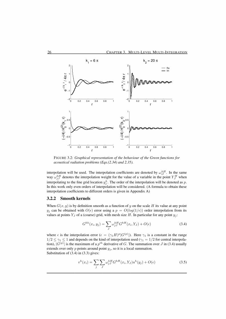
FIGURE 3.2: Graphical representation of the behaviour of the Green functions foracoustical radiation problems (Eqs.(2.34) and 2.35).
interpolation will be used. The interpolation coefficients are denoted by ωhHiI . In the same
way ωhHjJ denotes the interpolation weight for the value of a variable in the point Y H
J wheninterpolating to the fine grid location yh
j . The order of the interpolation will be denoted as p.In this work only even orders of interpolation will be considered. (A formula to obtain theseinterpolation coefficients to different orders is given in Appendix A)
3.2.2 Smooth kernelsWhen G(x, y) is by definition smooth as a function of y on the scale H its value at any pointyj can be obtained with O(ε) error using a p = O(log(1/ε)) order interpolation from itsvalues at points YJ of a (coarse) grid, with mesh size H . In particular for any point yj :
Ghh(xi, yj) =∑
J
ωhHjJ GhH(xi, YJ ) + O(ε) (3.4)
where ε is the interpolation error (ε = (γ1H)p|G(p)|). Here γ1 is a constant in the range1/2 ≤ γ1 ≤ 1 and depends on the kind of interpolation used (γ1 = 1/2 for central interpola-tion), |G(p)| is the maximum of a pth derivative of G. The summation over J in (3.4) usuallyextends over only p points around point yj , so it is a local summation.Substitution of (3.4) in (3.3) gives:
vh(xi) =∑
j
∑
J
ωhHjJ GhH(xi, YJ )uh(yj) + O(ε) (3.5)
§3.2. MULTILEVEL MULTI-INTEGRATION: BASIC ALGORITHM 27
Changing the order of summation yields:
vh(xi) =∑
J
GhH(xi, YJ )UH(YJ ) + O(ε) (3.6)
where
UH(YJ ) =∑
j
ωhHjJ uh(yj) (3.7)
As the summation over j (for each J) in (3.5) is a local summation over O(p) points alsothe summation over J for each j in (3.7) is also a local summation over O(2p) points whenH = 2h.
The change of order of summation going from (3.5) to (3.6) is the first crucial step in thealgorithm. Its effect is that a fine grid summation over index j is replaced by a coarse gridsummation over index J .
Summarizing, when Ghh(x, y) is smooth as a function of y the computation of vh(xi)by summation over all yj at the expense of an O(ε) error can be replaced by a coarse gridsummation (3.6) over all YJ of “injected” values Ghh(xi, yj) (GhH(xi, YJ ) ≡ Ghh(xi, y2J ))multiplied with collected charges UH(YJ ) defined by (3.7). This latter operation is referredto as anterpolation of uh(yj), since it is the adjoint of the interpolation of (3.4) [14].
Next, assume that Ghh(x, y) is also a smooth function of x on the scale H . In that casefor any xi up to O(ε) error Ghh(xi, y) can be obtained by interpolation from its values on acoarse grid XI with mesh size H .
Ghh(xi, yj) =∑
I
ωhHiI GHh(XI , yj) + O(ε) (3.8)
For a p-order interpolation the error is defined by ε = (γ1H)p|G(p)|. Often p = p can beused and ε = ε. For each i the summation over I is a local summation involving only pterms. This is the second crucial step in the algorithm. This second step implies that it isnot necessary to compute the transform in all points of the fine grid xi. Permitting a certainerror that can be controlled by the order of interpolation it is sufficient to only compute thesummations in coarse grid points, and then obtain the value in all points of a finer grid bymeans of interpolation.
The result of both steps is that, up to O(ε) error, the computation of vh(xi) in all evaluationgrid points xi involving a summation over all integration grid points yj can be replaced by:
(i) Anterpolation:UH(YJ ) =
∑
j
ωjJuh(yj) (3.9)
(ii) Injection of the kernel:
GHH(XI , YJ ) = Ghh(x2I , y2J ) (3.10)
(iii) Coarse grid summation:
V H(XI) =∑
J
GHH(XI , YJ )UH(YJ ) (3.11)
28 CHAPTER 3. MULTI-LEVEL MULTI-INTEGRATION
JU (Y ) =k−1 k2Jω
2JΣ k−1
2JkJ U (Y )
Level
G (X ,Y ) =
Ik−12I
k
2I
ω
k−2 (2H)
k−1 (H)
k (h)
V (X ))k−12IΣ
G (X ,Y )JIk−1k−1 k
IV (X ) =k
2I 2Jk
G (X ,Y )JΣ 1 1
I JIV (Y ) =1 1U (Y )J
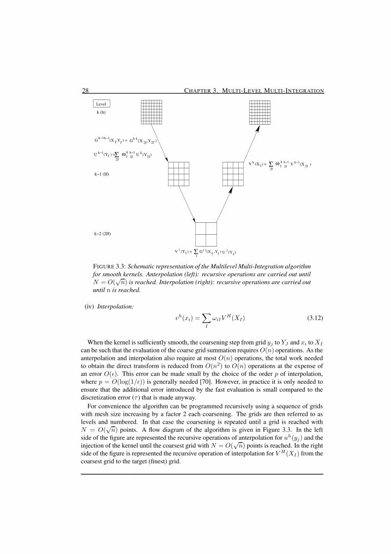
FIGURE 3.3: Schematic representation of the Multilevel Multi-Integration algorithmfor smooth kernels. Anterpolation (left): recursive operations are carried out untilN = O(
√n) is reached. Interpolation (right): recursive operations are carried out
until n is reached.
(iv) Interpolation:
vh(xi) =∑
I
ωiIVH(XI) (3.12)
When the kernel is sufficiently smooth, the coarsening step from grid yj to YJ and xi to XI
can be such that the evaluation of the coarse grid summation requires O(n) operations. As theanterpolation and interpolation also require at most O(n) operations, the total work neededto obtain the direct transform is reduced from O(n2) to O(n) operations at the expense ofan error O(ε). This error can be made small by the choice of the order p of interpolation,where p = O(log(1/ε)) is generally needed [70]. However, in practice it is only needed toensure that the additional error introduced by the fast evaluation is small compared to thediscretization error (τ ) that is made anyway.
For convenience the algorithm can be programmed recursively using a sequence of gridswith mesh size increasing by a factor 2 each coarsening. The grids are then referred to aslevels and numbered. In that case the coarsening is repeated until a grid is reached withN = O(
√n) points. A flow diagram of the algorithm is given in Figure 3.3. In the left
side of the figure are represented the recursive operations of anterpolation for uh(yj) and theinjection of the kernel until the coarsest grid with N = O(
√n) points is reached. In the right
side of the figure is represented the recursive operation of interpolation for V H(XI) from thecoarsest grid to the target (finest) grid.
§3.2. MULTILEVEL MULTI-INTEGRATION: BASIC ALGORITHM 29
0
0
|x−y|
← mh →|
Gh(x,y)ωhHGH(x,y)Interp. Error
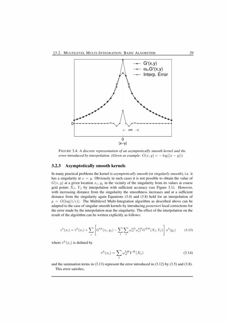
FIGURE 3.4: A discrete representation of an asymptotically smooth kernel and theerror introduced by interpolation. (Given as example: G(x, y) = − log(|x − y|))
3.2.3 Asymptotically smooth kernels
In many practical problems the kernel is asymptotically smooth (or singularly smooth), i.e. ithas a singularity at x = y. Obviously in such cases it is not possible to obtain the value ofG(x, y) at a given location xi, yj in the vicinity of the singularity from its values at coarsegrid points XI , YJ by interpolation with sufficient accuracy (see Figure 3.1). However,with increasing distance from the singularity the smoothness increases and at a sufficientdistance from the singularity again Equations (3.4) and (3.8) hold for an interpolation ofp = O(log(1/ε)). The Multilevel Multi-Integration algorithm as described above can beadapted to the case of singular smooth kernels by introducing posteriori local corrections forthe error made by the interpolation near the singularity. The effect of the interpolation on theresult of the algorithm can be written explicitly as follows:
vh(xi) = v
h(xi) +X
j
"
Ghh(xi, yj) −
X
I
X
J
ωhHiI ω
hHjJ G
HH(XI , YJ)
#
uh(yj) (3.13)
where vh(xi) is defined by
vh(xi) =∑
I
ωhHiI V H(XI) (3.14)
and the summation terms in (3.13) represent the error introduced in (3.12) by (3.5) and (3.8).This error satisfies,
30 CHAPTER 3. MULTI-LEVEL MULTI-INTEGRATION
Ghh(xi, yj) −
X
I
X
J
ωhHiI ω
hHjJ G
HH(XI , YJ ) =
0 xh = XH and yh = Y H
O(ε) |xh − yh| ≥ mh(3.15)
Choosing m sufficiently large the error due to the interpolation of the kernel (in both x andy) can be made small compared to the discretization error. The error introduced in the region|x − y| ≤ mh can be computed and added as a local correction, i.e. the summation over j in(3.13) extending over the range |x − y| ≤ mh.
Summarizing, (3.12) up to an error O(ε) can be written as,
vh(xi) = vh(xi) + vh(xi) (3.16)
where the correction term vh(xi) is defined by:
vh(xi) =∑
|i−j|≤m
[
Ghh(xi, yj) −∑
I
∑
J
ωhHiI ωhH
jJ GHH(XI , YJ )
]
uh(yj) (3.17)
For a given interpolation the correction kernel coefficients needed, see (3.15), can be pre-computed and stored. The total work of the algorithm now depends on m. The value of mcan be determined from a work-accuracy optimization: Setting the permissible error equal tothe discretization error τ find m such that the total work is minimized. An example of suchan analysis and details for the logarithm kernel G(x, y) = log |x − y| are given in [16] and[17].
The Multilevel Multi-Integration algorithm for an asymptotically smooth kernel is thusgiven by (3.9)-(3.12) steps (i) to (iv) followed by:
(v) Correction (3.16):vh(xi) = vh(xi) + vh(xi)
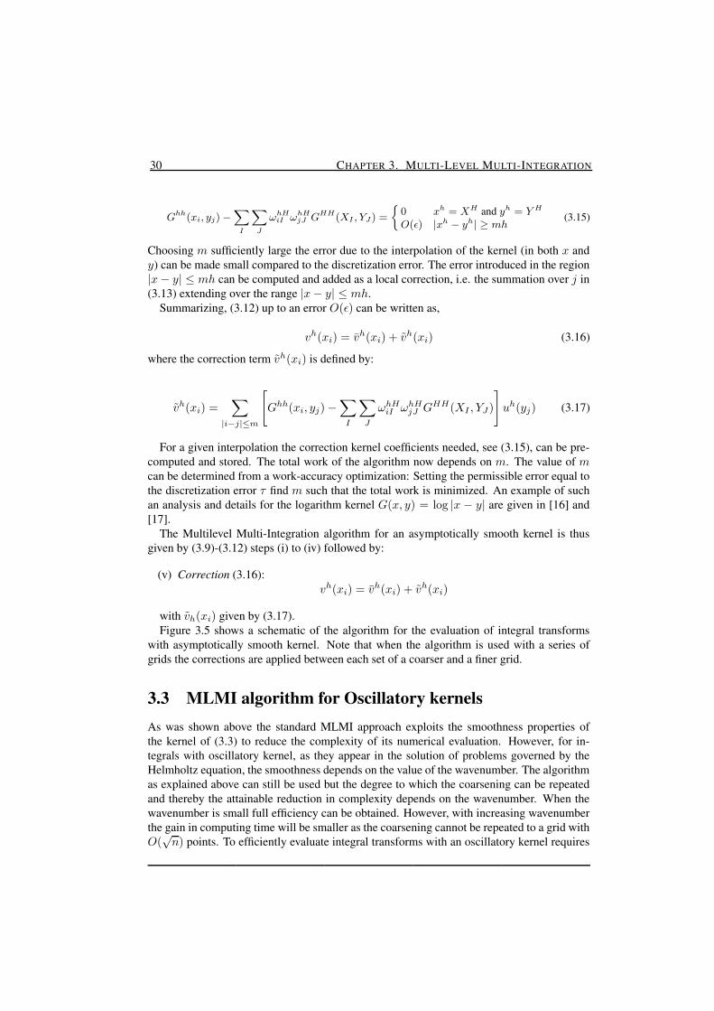
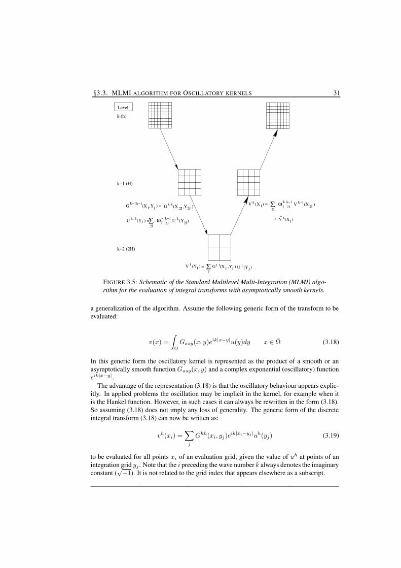
with vh(xi) given by (3.17).Figure 3.5 shows a schematic of the algorithm for the evaluation of integral transforms
with asymptotically smooth kernel. Note that when the algorithm is used with a series ofgrids the corrections are applied between each set of a coarser and a finer grid.
3.3 MLMI algorithm for Oscillatory kernelsAs was shown above the standard MLMI approach exploits the smoothness properties ofthe kernel of (3.3) to reduce the complexity of its numerical evaluation. However, for in-tegrals with oscillatory kernel, as they appear in the solution of problems governed by theHelmholtz equation, the smoothness depends on the value of the wavenumber. The algorithmas explained above can still be used but the degree to which the coarsening can be repeatedand thereby the attainable reduction in complexity depends on the wavenumber. When thewavenumber is small full efficiency can be obtained. However, with increasing wavenumberthe gain in computing time will be smaller as the coarsening cannot be repeated to a grid withO(
√n) points. To efficiently evaluate integral transforms with an oscillatory kernel requires
§3.3. MLMI ALGORITHM FOR OSCILLATORY KERNELS 31
2JΣ k−1
2Jk
I JJG (X ,Y )JΣ 1 1
J
2I 2JkkG (X ,Y )J
U (Y )ωJU (Y ) =k−1 k2J
U (Y )
V (X )~ k
2IΣI
I
k−2 (2H)
k−1 (H)
k (h)
+
Level
V (X ) = V (X )k−1
IV (Y ) =1 1
2Ik ω I
k−12I
k
Ik−1k−1G (X ,Y ) =
FIGURE 3.5: Schematic of the Standard Multilevel Multi-Integration (MLMI) algo-rithm for the evaluation of integral transforms with asymptotically smooth kernels.
a generalization of the algorithm. Assume the following generic form of the transform to beevaluated:
v(x) =
∫
Ω
Gasy(x, y)eik|x−y|u(y)dy x ∈ Ω (3.18)
In this generic form the oscillatory kernel is represented as the product of a smooth or anasymptotically smooth function Gasy(x, y) and a complex exponential (oscillatory) functioneik|x−y|.
The advantage of the representation (3.18) is that the oscillatory behaviour appears explic-itly. In applied problems the oscillation may be implicit in the kernel, for example when itis the Hankel function. However, in such cases it can always be rewritten in the form (3.18).So assuming (3.18) does not imply any loss of generality. The generic form of the discreteintegral transform (3.18) can now be written as:
vh(xi) =∑
j
Ghh(xi, yj)eik|xi−yj |uh(yj) (3.19)
to be evaluated for all points xi of an evaluation grid, given the value of uh at points of anintegration grid yj . Note that the i preceding the wave number k always denotes the imaginaryconstant (
√−1). It is not related to the grid index that appears elsewhere as a subscript.
32 CHAPTER 3. MULTI-LEVEL MULTI-INTEGRATION
Obviously for the case of an oscillatory kernel, the total kernel itself is not smooth. How-ever, the argument of the oscillatory part is a smooth function of x and y. Using this smooth-ness is the key idea in the generalization of the Multilevel Multi-Integration algorithm to thecase of oscillatory kernels.
Using the concept separation of directions the discrete transform is written as a series ofdiscrete subtransforms for a number of predefined directions. These subtransforms can berewritten in such a way that a kernel which is asymptotically smooth as a function of x and yappears. Its smoothness can then be used to obtain a fast evaluation.
3.3.1 Separation of directionsEquation (3.19) can be seen as a special case of a more general problem. This observationwill lead to the fast evaluation algorithm. Let xi be a point of the evaluation grid and a yj apoint of the integration grid where uh is given. The direction “vector” between xi and yj isnow determined by eij = (yj − xi)/|yj − xi|. Here |xi − yj |eij denotes the vector from thesender point yj to the receiver point xi. Let θij denote the angle of this vector, for example;in two dimensional problems eij = cos θij , sin θij. In (3.19) obviously the contribution ofa point yj to the transform at xi no depends on the direction between xi and yj . Howeverassume now that there were such an angular dependence and that it could be represented bydefining an angular radiation filter U(θ) and an angular reception filter G(θ), such that thegeneralized version of (3.19) is:
vh(x) =∑
j
G(xi, yj)G(θij)eik|xi−yj |U(θij)u
h(yj) (3.20)
The original task of evaluating (3.19) is exactly the same as equation (3.20) with U(θ) ≡ 1and G(θ) ≡ 1. We now define a grid of directions eβ ∈ σd = e ∈ IRd : |e| = 1 with σd
the unit sphere (circle), and eβ the associated base vectors, e.g. eβ = cos θβ , sin θβ for thetwo dimensional case (see Figure 3.6). It is assumed that the number of directions on the gridof directions is λ and the mesh size on this grid δθ = 2π/λ.
Now assume that U and G are smooth as a function of θ. This is obviously true for ourproblem. For any function that is smooth on the scale of the mesh size on the grid of directionsits value for a given direction θ can be obtained accurately by a pth-order interpolation fromits value at the directions on the grid. In particular,
U(θ) =∑
m∈s(e)
ws(e)m (e)U(θm) + O(ε) (3.21)
G(θ) =∑
l∈s(e)
ws(e)l (e)U(θl) + O(ε) (3.22)
where ws(e)l (e) and w
s(e)m (e) represent the interpolation weights of the value at a given base
vector l and m, respectively, into the result for a given e (see Appendix A). s(e) denotes theset of p base directions involved in the pth-order interpolation to the direction e. Preferablyit should be chosen such that e is central to the set. Because of periodicity the interpolationis well defined even if the number of directions is smaller than p. Even for the case λ = 1 ofa single direction it is well-defined as then w
s(e)λ (e) ≡ 1. Finally, the error ε is clearly zero
for the case of a constant function.

§3.3. MLMI ALGORITHM FOR OSCILLATORY KERNELS 33
G(θij)
U(θij) ije
1e
e0e2 xi
yj
1
λm=e
e
2e 0
l= λe
e
FIGURE 3.6: Schematic representation of the grid of directions for um(yj) and vl(xi).
Substitution of (3.21) and (3.22) to determine the value of G(θij) and U(θij) in Equa-tion (3.20) gives:
vh(xi) =∑
j
G(xi, yj)∑
l∈sij
wsij
l (eij)G(θl)eik|xi−yj |
∑
m∈sij
wsijm (eij)U(θm)uh(yj) (3.23)
By defining
uhm(yj) = U(θm)uh(yj) (3.24)
and defining that ws(e)l (e) = 0 for l /∈ s(e) the original task of evaluation of (3.19) can now
be written as the evaluation of:
vh(xi) =∑
l
G(θl)vhl (xi) (3.25)
with
vhl (xi) =
∑
j
Ghh(xi, yj)eik|xi−yj |w
sij
l (eij)∑
m∈sij
wsijm (eij)u
hm(yj) (3.26)
for 1 ≤ λ. So the generalized task is now to the evaluate (3.26) for l = 1, ..., λ. Note that theoriginal task (3.19) corresponds to the special case λ = 1.
3.3.2 One-dimensional scheme
To illustrate how the separation of directions introduced above can lead to a fast evaluationalgorithm, first consider a one-dimensional case. The general representation (3.26) can nowbe written in the form of only two directions (positive and negative) from xi.
34 CHAPTER 3. MULTI-LEVEL MULTI-INTEGRATION
eij =
+1 yj ≥ xi
−1 yj < xi(3.27)
The set of directions sij used in the interpolation to eij by definition consists of only onedirection and the interpolation weights are given by:
wsij
l (eij) =
1 eij = sij
0 eij 6= sijand wsij
m (eij) =
1 eij = sij
0 eij 6= sij(3.28)
Substituting (3.27) and (3.28) into (3.26), the generalization of the integral transform for onedimensional problems can be rewritten as:
vhl (xi) =
∑
j
Ghh(xi, yj)eik|xi−yj |uh
m(yj) l = m
0 otherwise(3.29)
Because (3.29) is defined for only two directions, we can introduce a simplified notation(+) and (-) to denote the directions that l and m can take: when x − y ≥ 0 the direction isdefined (+) when x − y < 0 it is defined (-). The function eik|x−y| in (3.29) can be split interms of x and y. The task (3.19) can now be rewritten as the computation of:
vh(xi) = e−ikxivh+(xi) + eikxivh
−(xi) (3.30)
where,
vh+(xi) =
∑
j
Ghh+ (xi, yj)u
h+(yj) (3.31)
vh−(xi) =
∑
j
Ghh− (xi, yj)u
h−(yj), (3.32)
with
G+(x, y) =
G(x, y) y ≥ x,0 y < x,
(3.33)
G−(x, y) =
0 y > x,G(x, y) y ≤ x, (3.34)
and,
uh+(yj) = eikyj uh(yj) (3.35)
uh−(yj) = e−ikyj uh(yj) (3.36)
The result is that the evaluation of the discrete transform with oscillatory kernel is nowrewritten into the task of evaluating two subtransforms, the summations (3.31) and (3.32),
§3.3. MLMI ALGORITHM FOR OSCILLATORY KERNELS 35
with each an asymptotically smooth kernel. Each of these summations can be evaluatedseparately using the algorithm described in Section 3.2.3, so that the evaluation of (3.19) canbe carried out by the following steps:
(i) Separate uh in (+) and (-) directions: (3.35) and (3.36)
(ii) Perform the MLMI algorithm for (+) and (-) directions: (3.31) and (3.32)
(iii) Combine vh+ and vh
− to vh: (3.30)
So, for a one dimensional problem the oscillatory part of the kernel can be fully incorpo-rated in the function v and u and no special algorithm is needed for the fast evaluation. Thetotal work involved in the fast evaluation for the oscillatory kernels is now twice the totalwork involved in the fast evaluation with a singular smooth kernel. So, for n points xi and npoints yj the total work is O(n log n).
3.3.3 Two and Three-dimensional schemeThe one-dimensional case illustrated the principle of separation of directions very clearly.The separation of directions leads to 2 subtransforms which each have a smooth or singularsmooth kernel. The principle for higher dimensional cases is the same. A series of subtran-forms appears. However, the separation of directions cannot be made so explicit that theoscillatory behaviour in x can be taken outside the summation. As a result the higher dimen-sional algorithm appears much more complex. In this case for each combination of directionsl, m a singular smooth kernel is obtained from the original kernel by multiplying it with anoscillatory function. The principle is as follows: Consider the function eik|x−y| in the one-dimensional case and assume x − y > 0. When multiplied by e−ikxeiky, it can be written aseik(|x−y|−x+y)eikye−ikx. Obviously the function eik(|x−y|−x+y) for the region (x − y) > 0is smooth in terms of x and y.
Now consider the two-dimensional case. The oscillatory term is written as:
eik|x−y| = eik(|x−y|+elx−emy)e−ikelxeikemy (3.37)
where em and el are a set of base vectors from the grid of directions. Substitution of (3.37)in (3.26) gives:
vhl (xi) =
∑
j
∑
m∈sij
Ghhijlm(xi, yj)e
ik(emyj−elxi)uhm(yj) (3.38)
with:
Gijlm(x, y) = G(x, y)eik(|x−y|+elx−emy) × wsij
l (x, y)wsijm (x, y) (3.39)
Now, for any combination of l and m, (3.39) is an asymptotically smooth function interms of x and y. Here, the interpolation weights plays a crucial role too. For given direc-tions m and l the exponential function is smooth in a region of the domain. The smooth-ness in the remaining part of the domain turns from the product of the interpolation weightsw
sij
l (x, y)wsijm (x, y) vanishing.
In the Figure 3.7 an illustration is given of the behaviour of the discrete function (3.39) forthe two-dimensional case, fixed index l = 0 (θl = 0) and m = 0 (θm = 0), the variable xi
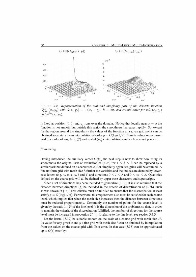
36 CHAPTER 3. MULTI-LEVEL MULTI-INTEGRATION
a) IRe(Gijlm(x, y)) b) IIm(Gijlm(x, y))
−1−0.5
00.5
1
−1−0.5
00.5
10
0.01
0.02
0.03
0.04
x−x‘y−y‘ −1−0.5
00.5
1
−1−0.5
00.5
1
0
2
4
6
8
10x 10
−3
x−x‘y−y‘
FIGURE 3.7: Representation of the real and imaginary part of the discrete functionGhh
ijlm(xi, yj) with G(xi, yj) = 1/|xi − yj |, k = 2π, and second order for wsijm (xi, yj)
and wsij
l (xi, yj).
is fixed at position (0, 0) and yj runs over the domain. Notice that locally near x = y thefunction is not smooth but outside this region the smoothness increases rapidly. So, exceptfor the region around the singularity the values of the function at a given grid point can beobtained accurately by an interpolation of order p = O(log(1/ε)) from its values on a coarsergrid (the order of angular (pth
θ ) and spatial (pthxy) interpolation can be chosen independent).
Coarsening
Having introduced the auxillary kernel Ghhijlm the next step is now to show how using its
smoothness the original task of evaluation of (3.26) for 1 ≤ l ≤ λ can be replaced by asimilar task but defined on a coarser scale. For simplicity again two grids will be assumed. Afine uniform grid with mesh size h further the variables and the indices are denoted by lower-case letters (e.g. v, u, x, y, i and j) and directions 0 ≤ l ≤ λ and 0 ≤ m ≤ λ. Quantitiesdefined on the coarse grid will all be defined by upper-case characters and superscripts.
Since a set of directions has been included to generalize (3.19), it is also required that thedistance between directions (δ) be included in the criteria of discretization of (3.26), suchas was shown in [14]. This criteria must be fulfilled to ensure that the discretization at leastsatisfy p = O(log(1/ε)). Furthermore, this requirement also must be satisfied for each coarselevel, which implies that when the mesh size increases then the distance between directionsmust be reduced proportionately. Commonly the number of points for the coarse level isgiven by the ratio 1 : 2d of the fine level (d is the dimension of the problem), so that, in orderto mantain the criteria of the discretization fullfilled, the number of directions for the coarselevel must be increased in proportion 2d−1 : 1 relative to the fine level, see section 3.3.3.
Let the kernel (3.39) be suitable smooth on the scale of a coarse grid with mesh size H .Its value for any given x and y a fine grid with mesh size h can be obtained by interpolationfrom the values on the coarse grid with O(ε) error. In that case (3.38) can be approximatedup to O(ε) error by:
§3.3. MLMI ALGORITHM FOR OSCILLATORY KERNELS 37
vhl (xi) =
∑
j
∑
m∈sij
∑
I∈σi
∑
J∈σj
ωhHiI ωhH
jJ GHHijlm(XI , YJ )eik(emyj−elxi)uh
m(yj) (3.40)
where σi and σj are the sets of points in the neighbourhood of xi and yj used by the in-terpolation. This equation will now be re-written into a coarse grid representation. For thecase of a smooth or asymptotically smooth kernel, this was quite straightforward since it onlyinvolved a change in the order of the summations (see Equation (3.6)). In this case it is a littlemore complex because exponential terms appear as well as their relation with the directionsm and l. Using (3.39) and re-arranging terms, (3.40) can be written as:
vhl (xi) =
∑
I∈σi
ωhHiI eikel(XI−xi)
∑
j
∑
J∈σj
ωhHjJ GHH(XI , YJ )eik|XI−YJ |w
sij
l (XI , YJ )
∑
m∈sij
wsijm (XI , YJ )eikem(yj−YJ )uh
m(yj) (3.41)
Taking a close look at this equation it can be seen that the last summation∑
m∈sijinvolv-
ing the weights wsijm (XI , YJ ) is in fact an interpolation taking place from the fine grid of
directions to the direction EIJ of the product of the functions uhm(yj) and eikem(yj−YJ ). As
shown in Brandt [14], both uhm(yj) and eikem(yj−YJ ) are smooth on the grid of directions (i.e.
as a function of m). As a result their interpolation from emm∈sijcan be replaced, to O(ε)
accuracy, by an interpolation from any other close subset of em, so that in (3.41) the sum-mation
∑
m∈sijw
sijm (XI , YJ ) could for example be replaced by the
∑
m∈sEijw
s(Eij)m (EIJ).
So as well the interpolation could be replaced by an interpolation from the set EMM∈SIJ,
provided uhm(yj) were defined on EM instead of on em. However, using the fact that
uhm(yj) is suitably smooth on em it can be interpolated to the coarse grid of directions
EM by defining uhM (yj),
uhM (yj) =
∑
m∈sEM
ws(EM )m (EM)uh
m(yj) (3.42)
As a reminder, the number of directions on the coarse grid is 2d−1 as large as on the fine grid,so this is indeed interpolation. As a result (3.41) can now be replaced by
vhl (xi) =
∑
I∈σi
ωhHiI eikel(XI−xi)
∑
j
∑
J∈σj
ωhHjJ GHH(XI , YJ )eik|XI−YJ |w
sij
l (EIJ)
∑
M∈SIJ
WSIJ
M (EIJ)eikem(yj−YJ )uhM (yj) (3.43)
In a similar way (see Brandt [14]), the final result of the algorithm should, up to a per-missible O(ε) error, not change when the interpolation coefficients w
sij
l (EIJ) in (3.43) arereplaced by pth-order interpolation coefficients to the same EIJ from any (other) closeset. In particular they can be replaced by coefficients of pth-order interpolation using theset EL; i.e. a pth-order interpolation from el to EL followed by a pth-order in-terpolation from EL to EIJ . This implies that the term w
sij
l (EIJ) in (3.43) can be re-placed by
∑
L ws(EL)l (EL)W
S(EIJ )L (EIJ), where the summation is over all L such that(s.t.)
l ∈ s(EL). Introducing this replacement one obtains:
38 CHAPTER 3. MULTI-LEVEL MULTI-INTEGRATION
vhl (xi) =
∑
I∈σ
ωhHiI eikel(XI−xi)V H
l (XI) (3.44)
where
V Hl (XI) =
∑
L s.t.
l ∈ s(EL)
ws(EL)l (EL)V H
L (XI) (3.45)
V HL (XI) =
∑
J
GHH(XI , YJ )eik|XI−YJ |WSIJ
L (EIJ)∑
M∈SIJ
WSIJ
M (EIJ)UHM (YJ ) (3.46)
UHM (YJ ) =
∑
j s.t.
J ∈ σj
eikEM (yj−YJ )uhM (yj) (3.47)
(3.46) is exactly a coarse-grid version of (3.26). So, the coarsening process is complete. Thetask of the evaluation of (3.26) on the target grid h can thus be replaced by the evaluation ofthe coarse grid problem (3.46) and a number of intergrid operations in space and directions.The different steps are described below and the entire process is summarized in Figure 3.8for a two-dimensional problems.
(i) Angular density interpolation:
Calculate uhM (yj) in all points yj for all coarse grid directions M = 1, ..., Λ using
Eq. (3.47).
(ii) Density oscillatory anterpolation:
Calculate UHM (YJ) in all coarse grid points for all coarse grid directions M = 1, ..., Λ,
using Eq. (3.42).
(iii) Coarse grid summation:
Compute V HL (XI) defined by (3.46) for all coarse grid points XI for all coarse grid
directions L = 1, ..., Λ.
(iv) Angular field anterpolation:
Calculate V Hl (XI) for each fine grid direction l = 1, ..., λ by anterpolation on the grid
of directions as defined by Eq. (3.45).
(v) Field oscillatory interpolation:
Calculate vhl (xi) for l = 1, ..., λ in all fine grid points xi using Eq. (3.44)
Notice, that as the number of directions on the coarser grid is 2d−1 as large, but the numberof nodes 2d times smaller, when applied recursively, the algorithm will certainly lead toa reduction of the total amount of work when the number of points on the finest grid issufficiently large.
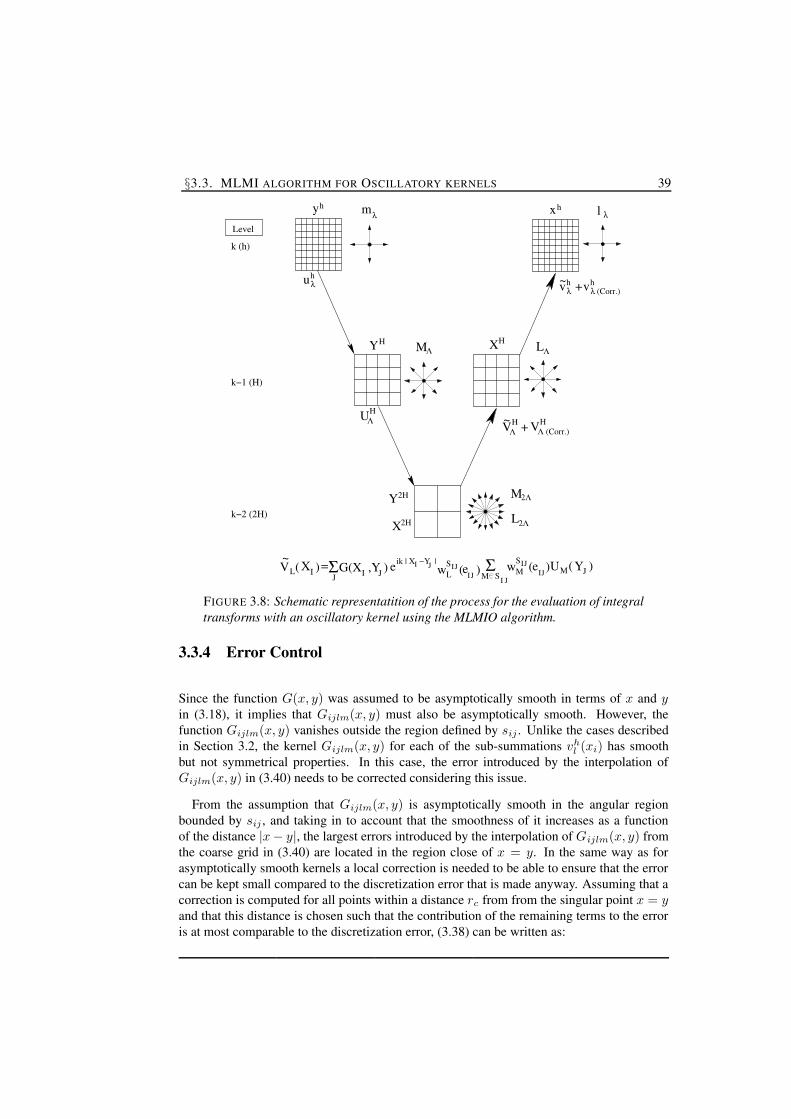
§3.3. MLMI ALGORITHM FOR OSCILLATORY KERNELS 39
λ (Corr.)
V +Λ
vhv +λh
H
Je I
VΛH
(Corr.)
ik | X −Y |
H
2H
Y2H
uλ
UΛ
h
M2Λ
L2Λ
Σe MS J
IJw ( )I
Jw ( )U J( )YM
I eJIJ
SIL =( )V
M S I J
X Σ
~
IG(X ,Y )L
~
J
k (h)
k−1 (H)
k−2 (2H)
~
X
m l λ
L
λ
Λ
xh
XHH MΛ
yh
Y
Level
FIGURE 3.8: Schematic representatition of the process for the evaluation of integraltransforms with an oscillatory kernel using the MLMIO algorithm.
3.3.4 Error Control
Since the function G(x, y) was assumed to be asymptotically smooth in terms of x and yin (3.18), it implies that Gijlm(x, y) must also be asymptotically smooth. However, thefunction Gijlm(x, y) vanishes outside the region defined by sij . Unlike the cases describedin Section 3.2, the kernel Gijlm(x, y) for each of the sub-summations vh
l (xi) has smoothbut not symmetrical properties. In this case, the error introduced by the interpolation ofGijlm(x, y) in (3.40) needs to be corrected considering this issue.
From the assumption that Gijlm(x, y) is asymptotically smooth in the angular regionbounded by sij , and taking in to account that the smoothness of it increases as a functionof the distance |x− y|, the largest errors introduced by the interpolation of Gijlm(x, y) fromthe coarse grid in (3.40) are located in the region close of x = y. In the same way as forasymptotically smooth kernels a local correction is needed to be able to ensure that the errorcan be kept small compared to the discretization error that is made anyway. Assuming that acorrection is computed for all points within a distance rc from from the singular point x = yand that this distance is chosen such that the contribution of the remaining terms to the erroris at most comparable to the discretization error, (3.38) can be written as:
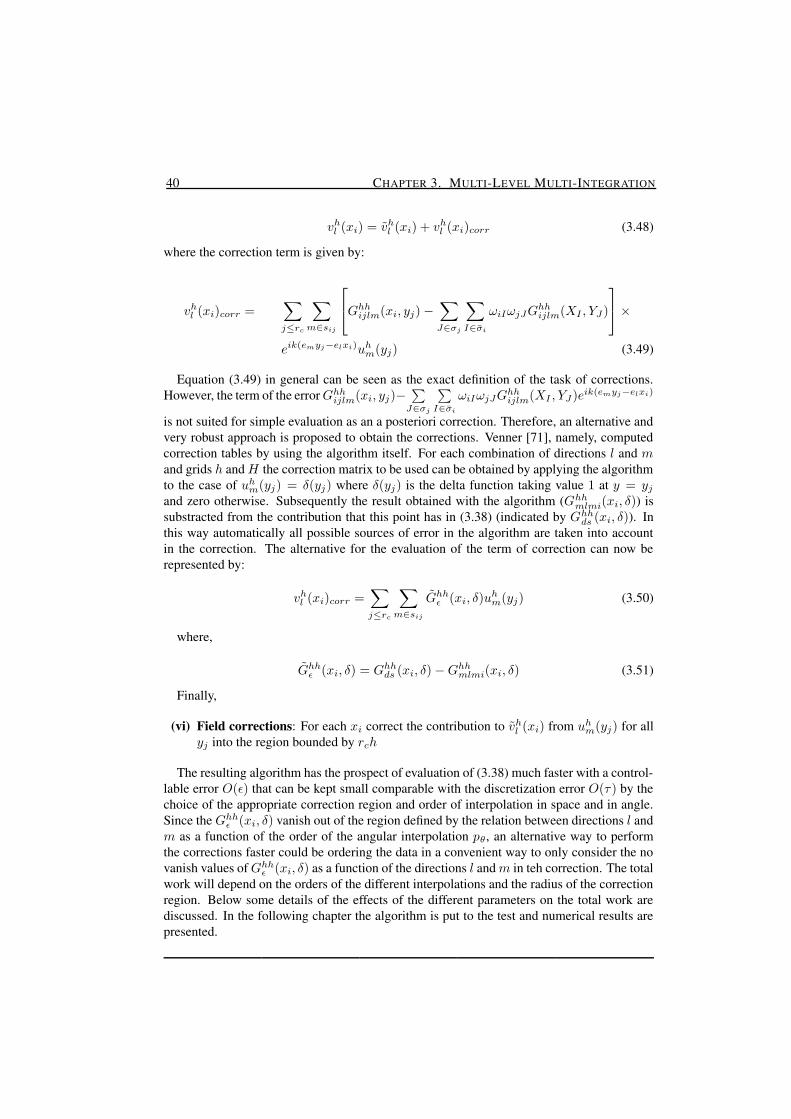
40 CHAPTER 3. MULTI-LEVEL MULTI-INTEGRATION
vhl (xi) = vh
l (xi) + vhl (xi)corr (3.48)
where the correction term is given by:
vhl (xi)corr =
∑
j≤rc
∑
m∈sij
Ghhijlm(xi, yj) −
∑
J∈σj
∑
I∈σi
ωiIωjJGhhijlm(XI , YJ )
×
eik(emyj−elxi)uhm(yj) (3.49)
Equation (3.49) in general can be seen as the exact definition of the task of corrections.However, the term of the error Ghh
ijlm(xi, yj)−∑
J∈σj
∑
I∈σi
ωiIωjJGhhijlm(XI , YJ )eik(emyj−elxi)
is not suited for simple evaluation as an a posteriori correction. Therefore, an alternative andvery robust approach is proposed to obtain the corrections. Venner [71], namely, computedcorrection tables by using the algorithm itself. For each combination of directions l and mand grids h and H the correction matrix to be used can be obtained by applying the algorithmto the case of uh
m(yj) = δ(yj) where δ(yj) is the delta function taking value 1 at y = yj
and zero otherwise. Subsequently the result obtained with the algorithm (Ghhmlmi(xi, δ)) is
substracted from the contribution that this point has in (3.38) (indicated by Ghhds (xi, δ)). In
this way automatically all possible sources of error in the algorithm are taken into accountin the correction. The alternative for the evaluation of the term of correction can now berepresented by:
vhl (xi)corr =
∑
j≤rc
∑
m∈sij
Ghhε (xi, δ)u
hm(yj) (3.50)
where,
Ghhε (xi, δ) = Ghh
ds (xi, δ) − Ghhmlmi(xi, δ) (3.51)
Finally,
(vi) Field corrections: For each xi correct the contribution to vhl (xi) from uh
m(yj) for allyj into the region bounded by rch
The resulting algorithm has the prospect of evaluation of (3.38) much faster with a control-lable error O(ε) that can be kept small comparable with the discretization error O(τ) by thechoice of the appropriate correction region and order of interpolation in space and in angle.Since the Ghh
ε (xi, δ) vanish out of the region defined by the relation between directions l andm as a function of the order of the angular interpolation pθ, an alternative way to performthe corrections faster could be ordering the data in a convenient way to only consider the novanish values of Ghh
ε (xi, δ) as a function of the directions l and m in teh correction. The totalwork will depend on the orders of the different interpolations and the radius of the correctionregion. Below some details of the effects of the different parameters on the total work arediscussed. In the following chapter the algorithm is put to the test and numerical results arepresented.
§3.4. ESTIMATION OF COMPLEXITY 41
3.4 Estimation of complexitySince that the algorithm for oscillatory kernels above was derived using two kinds of auxiliarygrids (spatial and angular), it is possible to take independent p the order of interpolation oneach grid such that they can be represented as pθ for the angular and ps for the spatial orderof interpolation. So an estimation of the computational work can be done as a function ofthese two parameters and the correction parameter rc.
Considering that one operation is defined as one addition and one multiplication, then thework done by the algorithm can be determined by:
1. Angular interpolation and anterpolation (steps i and iv): O(λnpθ)
2. Spatial anterpolation and interpolation (steps ii and v): O(λnps) when the anterpola-tion/interpolation can be done one dimension at a time, and O(λnpd
s) otherwise.
3. Summation at the coarsest level (step iii): This work can be neglected due to the eval-uation of (3.46) on the coarsest level is performed in only O(2
√npθ) operations.
4. Correction (step vi): A estimation of the work for the corrections is given by O(λnrdcpθ)
since that for each i and l involves pθ directions of m and a region bounded by rc inthe vicinity of the singularity (x = y).
Notice that the most expensive computational task above is related with the operation ofcorrection due to the error introduced by the interpolation close to the singularity. In orderto minimize this work an optimization as a function of the parameters pθ, pxy and rc isdesirable. Examples of optimization can be found in [16] and [17]. It should be an item forfurther research.

42 CHAPTER 3. MULTI-LEVEL MULTI-INTEGRATION

4 CH
AP
TE
R
NUMERICAL RESULTS MLMIO
In this chapter results obtained with the Multilevel Multi-Integration algorithm are presentedfor a number of one- and two-dimensional model problems of integral transforms with os-cillatory kernel. The performance of the algorithm is measured by means of comparing theapproximation to the discrete transform that is obtained with the exact analytical solution andwith the result obtained using single grid simple matrix multiplication. In various ways itis shown that the generalization of the MLMI algorithm using separation of directions in-deed works and enables fast evaluation of discrete integral transform with oscillatory kernelwith performance independent of the wavenumber. Finally for reference the performance ofthe algorithm for some of the model problems is compared with the performance of an FFTalgorithm.
4.1 One dimension (G(x, y) smooth)The first model problem is the evaluation of the integral transform (3.18) for one a dimen-sional case with G(x, y) a smooth function of x and y:
v(x) =
∫ 1
−1
G(x, y)eik|x−y|u(y)dy, x ∈ [−1, 1] (4.1)
where,
G(x, y) = cos(y − x) and u(y) = 1 − y2, (4.2)
for different values of the wave number (k).For this case the analytical solution is known, see Appendix B, and will be used to evaluate
the accuracy of the numerical results obtained.
4.1.1 Discretization
The integral transform (4.1) was discretized as descibed in section 3.3. Here a constantmeshsize h is assumed. uh(yj) and vh(xi) are the discrete approximations to u and v on thegrid. The numerical approximation of (4.1) was done in two ways:

44 CHAPTER 4. NUMERICAL RESULTS MLMIO
i) Single Matrix MultiplicationIn this case, the integral transform (4.1) was discretized as follows: In each interval [yj −h2 , yj + h
2 ] the function is approximated by a piecewise constant function with the valueuh(yj). Subsequently, the contribution of the interval to vh(x) is defined as:
δjvh(x) =
[
∫ yj+h2
yj−h2
G(x, y)eik|x−y|dy
]
uh(yj). (4.3)
Summing up the contributions of all integration intervals one obtains a discrete approximationto v given by the following single matrix multiplication:
vh(xi) =∑
j
Ghhosc(xi, yj) uh(yj) (4.4)
where the coefficients of the matrix (discrete kernel) Ghhosc are given by:
Ghhosc(xi, yj) =
∫ yj+h2
yj−h2
G(xi, y)eik|xi−y|dy (4.5)
These coefficients were computed numerically using a Gauss adaptive quadrature approachwith predefined accuracy ε = O(10−8). The discretization is of second order and the errorshould be insensitive to the wave number k.
ii) Separation of Directions (MLMIO)The second approach uses the separation of directions in MLMIO algorithm as described inthe previous chapter. The discrete representation of v is:
vh(xi) = e−ikxivh+(xi) + eikxivh
−(xi) (4.6)
where
vh+(xi) =
∑
j
Ghh+ (xi, yj)u
h+(yj) (4.7)
vh−(xi) =
∑
j
Ghh− (xi, yj)u
h−(yj) (4.8)
with,
Ghh+ (xi, yj) =
(A+ + B+)Ghh(xi, yj) j > i,A+ Ghh(xi, yj) j = i,0 j < i,
(4.9)
Ghh− (xi, yj) =
0 j > i,B− Ghh(xi, yj) j = i,(A− + B−)Ghh(xi, yj) j < i,
(4.10)
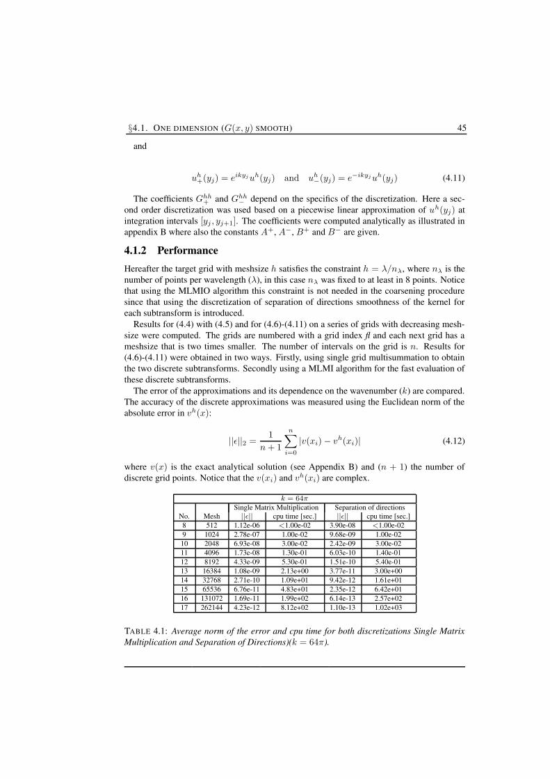
§4.1. ONE DIMENSION (G(x, y) SMOOTH) 45
and
uh+(yj) = eikyj uh(yj) and uh
−(yj) = e−ikyj uh(yj) (4.11)
The coefficients Ghh+ and Ghh
− depend on the specifics of the discretization. Here a sec-ond order discretization was used based on a piecewise linear approximation of uh(yj) atintegration intervals [yj , yj+1]. The coefficients were computed analytically as illustrated inappendix B where also the constants A+, A−, B+ and B− are given.
4.1.2 PerformanceHereafter the target grid with meshsize h satisfies the constraint h = λ/nλ, where nλ is thenumber of points per wavelength (λ), in this case nλ was fixed to at least in 8 points. Noticethat using the MLMIO algorithm this constraint is not needed in the coarsening proceduresince that using the discretization of separation of directions smoothness of the kernel foreach subtransform is introduced.
Results for (4.4) with (4.5) and for (4.6)-(4.11) on a series of grids with decreasing mesh-size were computed. The grids are numbered with a grid index fl and each next grid has ameshsize that is two times smaller. The number of intervals on the grid is n. Results for(4.6)-(4.11) were obtained in two ways. Firstly, using single grid multisummation to obtainthe two discrete subtransforms. Secondly using a MLMI algorithm for the fast evaluation ofthese discrete subtransforms.
The error of the approximations and its dependence on the wavenumber (k) are compared.The accuracy of the discrete approximations was measured using the Euclidean norm of theabsolute error in vh(x):
||ε||2 =1
n + 1
n∑
i=0
|v(xi) − vh(xi)| (4.12)
where v(x) is the exact analytical solution (see Appendix B) and (n + 1) the number ofdiscrete grid points. Notice that the v(xi) and vh(xi) are complex.
k = 64πSingle Matrix Multiplication Separation of directions
No. Mesh ||ε|| cpu time [sec.] ||ε|| cpu time [sec.]8 512 1.12e-06 <1.00e-02 3.90e-08 <1.00e-029 1024 2.78e-07 1.00e-02 9.68e-09 1.00e-0210 2048 6.93e-08 3.00e-02 2.42e-09 3.00e-0211 4096 1.73e-08 1.30e-01 6.03e-10 1.40e-0112 8192 4.33e-09 5.30e-01 1.51e-10 5.40e-0113 16384 1.08e-09 2.13e+00 3.77e-11 3.00e+0014 32768 2.71e-10 1.09e+01 9.42e-12 1.61e+0115 65536 6.76e-11 4.83e+01 2.35e-12 6.42e+0116 131072 1.69e-11 1.99e+02 6.14e-13 2.57e+0217 262144 4.23e-12 8.12e+02 1.10e-13 1.02e+03
TABLE 4.1: Average norm of the error and cpu time for both discretizations Single MatrixMultiplication and Separation of Directions)(k = 64π).
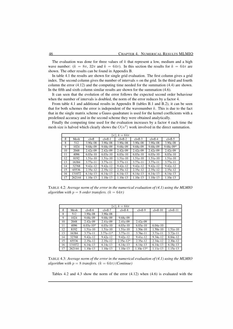
46 CHAPTER 4. NUMERICAL RESULTS MLMIO
The evaluation was done for three values of k that represent a low, medium and a highwave number: (k = 8π, 32π and k = 64π). In this section the results for k = 64π areshown. The other results can be found in Appendix B.
In table 4.1 the results are shown for single grid evaluation. The first column gives a gridindex. The second column gives the number of intervals n on the grid. In the third and fourthcolumn the error (4.12) and the computing time needed for the summation (4.4) are shown.In the fifth and sixth column similar results are shown for the summation (4.6).
It can seen that the evolution of the error follows the expected second order behaviourwhen the number of intervals is doubled, the norm of the error reduces by a factor 4.
From table 4.1 and additional results in Appendix B (tables B.1 and B.2), it can be seenthat for both schemes the error is independent of the wavenumber k. This is due to the factthat in the single matrix scheme a Gauss quadrature is used for the kernel coefficients with apredefined accuracy and in the second scheme they were obtained analytically.
Finally the computing time used for the evaluation increases by a factor 4 each time themesh size is halved which clearly shows the O(n2) work involved in the direct summation.
||ε||, k = 64πfl Mesh cl=fl cl=fl-1 cl=fl-2 cl=fl-3 cl=fl-4 cl=fl-58 512 3.90e-08 3.90e-08 3.90e-08 3.90e-08 3.90e-08 3.90e-089 1024 9.68e-09 9.68e-09 9.68e-09 9.68e-09 9.68e-09 9.68e-09*
10 2048 2.42e-09 2.42e-09 2.42e-09 2.42e-09 2.42e-09 2.42e-0911 4096 6.03e-10 6.03e-10 6.03e-10 6.03e-10 6.03e-10 6.03e-1012 8192 1.51e-10 1.51e-10 1.51e-10 1.51e-10 1.51e-10 1.51e-1013 16384 3.77e-11 3.77e-11 3.77e-11 3.77e-11 3.77e-11 3.77e-1114 32768 9.42e-12 9.42e-12 9.42e-12 9.42e-12 9.42e-12 9.42e-1215 65536 2.35e-12 2.35e-12 2.35e-12 2.35e-12 2.35e-12 2.35e-1216 131072 6.14e-13 6.14e-13 6.14e-13 6.14e-13 6.14e-13 6.14e-1317 262144 1.10e-13 1.10e-13 1.10e-13 1.10e-13 1.10e-13 1.10e-13
TABLE 4.2: Average norm of the error in the numerical evaluation of (4.1) using the MLMIOalgorithm with p = 8 order transfers. (k = 64π)
||ε||, k = 64πfl Mesh cl=fl-6 cl=fl-7 cl=fl-8 cl=fl-9 cl=fl-10 cl=fl-118 512 3.90e-08 3.90e-089 1024 9.68e-09 9.68e-09 9.68e-0910 2048 2.42e-09 2.41e-09 2.41e-09 2.42e-0911 4096 6.03e-10* 6.03e-10 6.03e-10 6.03e-10 6.04e-1012 8192 1.51e-10 1.51e-10 1.51e-10 1.50e-10 1.50e-10 1.51e-1013 16384 3.77e-11 3.77e-11* 3.77e-11 3.76e-11 3.71e-11 3.72e-1114 32768 9.42e-12 9.42e-12 9.42e-12 9.41e-12 9.34e-12 8.84e-1215 65536 2.35e-12 2.35e-12 2.35e-12* 2.35e-12 2.34e-12 2.30e-1216 131072 6.14e-13 6.14e-13 6.14e-13 6.14e-13 6.14e-13 6.18e-1317 262144 1.10e-13 1.10e-13 1.10e-13 1.10e-13* 1.11e-13 1.15e-13
TABLE 4.3: Average norm of the error in the numerical evaluation of (4.1) using the MLMIOalgorithm with p = 8 transfers. (k = 64π) (Continue)
Tables 4.2 and 4.3 show the norm of the error (4.12) when (4.6) is evaluated with the
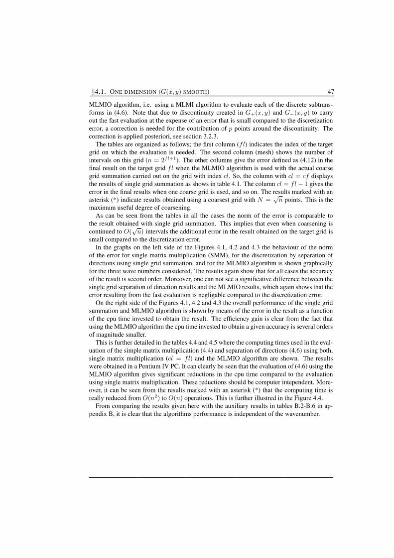
§4.1. ONE DIMENSION (G(x, y) SMOOTH) 47
MLMIO algorithm, i.e. using a MLMI algorithm to evaluate each of the discrete subtrans-forms in (4.6). Note that due to discontinuity created in G+(x, y) and G−(x, y) to carryout the fast evaluation at the expense of an error that is small compared to the discretizationerror, a correction is needed for the contribution of p points around the discontinuity. Thecorrection is applied posteriori, see section 3.2.3.
The tables are organized as follows; the first column (fl) indicates the index of the targetgrid on which the evaluation is needed. The second column (mesh) shows the number ofintervals on this grid (n = 2fl+1). The other columns give the error defined as (4.12) in thefinal result on the target grid fl when the MLMIO algorithm is used with the actual coarsegrid summation carried out on the grid with index cl. So, the column with cl = cf displaysthe results of single grid summation as shows in table 4.1. The column cl = fl − 1 gives theerror in the final results when one coarse grid is used, and so on. The results marked with anasterisk (*) indicate results obtained using a coarsest grid with N =
√n points. This is the
maximum useful degree of coarsening.As can be seen from the tables in all the cases the norm of the error is comparable to
the result obtained with single grid summation. This implies that even when coarsening iscontinued to O(
√n) intervals the additional error in the result obtained on the target grid is
small compared to the discretization error.In the graphs on the left side of the Figures 4.1, 4.2 and 4.3 the behaviour of the norm
of the error for single matrix multiplication (SMM), for the discretization by separation ofdirections using single grid summation, and for the MLMIO algorithm is shown graphicallyfor the three wave numbers considered. The results again show that for all cases the accuracyof the result is second order. Moreover, one can not see a significative difference between thesingle grid separation of direction results and the MLMIO results, which again shows that theerror resulting from the fast evaluation is negligable compared to the discretization error.
On the right side of the Figures 4.1, 4.2 and 4.3 the overall performance of the single gridsummation and MLMIO algorithm is shown by means of the error in the result as a functionof the cpu time invested to obtain the result. The efficiency gain is clear from the fact thatusing the MLMIO algorithm the cpu time invested to obtain a given accuracy is several ordersof magnitude smaller.
This is further detailed in the tables 4.4 and 4.5 where the computing times used in the eval-uation of the simple matrix multiplication (4.4) and separation of directions (4.6) using both,single matrix multiplication (cl = fl) and the MLMIO algorithm are shown. The resultswere obtained in a Pentium IV PC. It can clearly be seen that the evaluation of (4.6) using theMLMIO algorithm gives significant reductions in the cpu time compared to the evaluationusing single matrix multiplication. These reductions should be computer intependent. More-over, it can be seen from the results marked with an asterisk (*) that the computing time isreally reduced from O(n2) to O(n) operations. This is further illustred in the Figure 4.4.
From comparing the results given here with the auxiliary results in tables B.2-B.6 in ap-pendix B, it is clear that the algorithms performance is independent of the wavenumber.
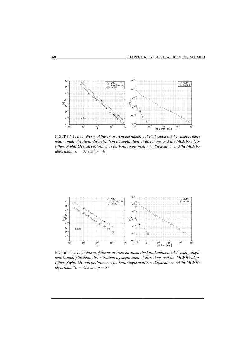
48 CHAPTER 4. NUMERICAL RESULTS MLMIO
101
102
103
104
105
10−11
10−10
10−9
10−8
10−7
10−6
10−5
10−4
n
||ε|| 2
k: 8 π
SMMDisc. Sep. Dir.MLMIO
10−2
10−1
100
101
102
10−11
10−10
10−9
10−8
10−7
10−6
cpu time [sec.]||ε
|| 2
SMMMLMIO
FIGURE 4.1: Left: Norm of the error from the numerical evaluation of (4.1) using singlematrix multiplication, discretization by separation of directions and the MLMIO algo-rithm. Right: Overall performance for both single matrix multiplication and the MLMIOalgorithm. (k = 8π and p = 8)
102
103
104
105
106
10−13
10−12
10−11
10−10
10−9
10−8
10−7
10−6
10−5
n
||ε|| 2
k: 32 π
SMMDisc. Sep. Dir.MLMIO
10−2
10−1
100
101
102
103
10−13
10−12
10−11
10−10
10−9
10−8
10−7
cpu time [sec.]
||ε|| 2
SMMMLMIO
FIGURE 4.2: Left: Norm of the error from the numerical evaluation of (4.1) using singlematrix multiplication, discretization by separation of directions and the MLMIO algo-rithm. Right: Overall performance for both single matrix multiplication and the MLMIOalgorithm. (k = 32π and p = 8)
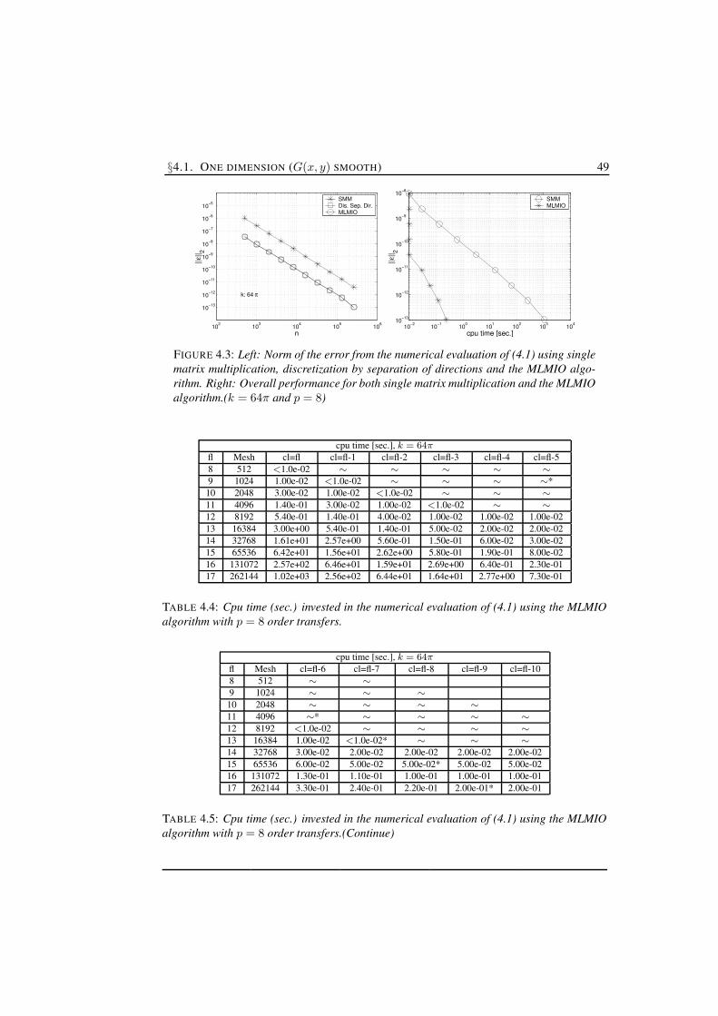
§4.1. ONE DIMENSION (G(x, y) SMOOTH) 49
102
103
104
105
106
10−13
10−12
10−11
10−10
10−9
10−8
10−7
10−6
10−5
n
||ε|| 2
k: 64 π
SMMDis. Sep. Dir.MLMIO
10−2
10−1
100
101
102
103
104
10−13
10−12
10−11
10−10
10−9
10−8
cpu time [sec.]
||ε|| 2
SMMMLMIO
FIGURE 4.3: Left: Norm of the error from the numerical evaluation of (4.1) using singlematrix multiplication, discretization by separation of directions and the MLMIO algo-rithm. Right: Overall performance for both single matrix multiplication and the MLMIOalgorithm.(k = 64π and p = 8)
cpu time [sec.], k = 64πfl Mesh cl=fl cl=fl-1 cl=fl-2 cl=fl-3 cl=fl-4 cl=fl-58 512 <1.0e-02 ∼ ∼ ∼ ∼ ∼9 1024 1.00e-02 <1.0e-02 ∼ ∼ ∼ ∼*10 2048 3.00e-02 1.00e-02 <1.0e-02 ∼ ∼ ∼11 4096 1.40e-01 3.00e-02 1.00e-02 <1.0e-02 ∼ ∼12 8192 5.40e-01 1.40e-01 4.00e-02 1.00e-02 1.00e-02 1.00e-0213 16384 3.00e+00 5.40e-01 1.40e-01 5.00e-02 2.00e-02 2.00e-0214 32768 1.61e+01 2.57e+00 5.60e-01 1.50e-01 6.00e-02 3.00e-0215 65536 6.42e+01 1.56e+01 2.62e+00 5.80e-01 1.90e-01 8.00e-0216 131072 2.57e+02 6.46e+01 1.59e+01 2.69e+00 6.40e-01 2.30e-0117 262144 1.02e+03 2.56e+02 6.44e+01 1.64e+01 2.77e+00 7.30e-01
TABLE 4.4: Cpu time (sec.) invested in the numerical evaluation of (4.1) using the MLMIOalgorithm with p = 8 order transfers.
cpu time [sec.], k = 64πfl Mesh cl=fl-6 cl=fl-7 cl=fl-8 cl=fl-9 cl=fl-108 512 ∼ ∼9 1024 ∼ ∼ ∼10 2048 ∼ ∼ ∼ ∼11 4096 ∼* ∼ ∼ ∼ ∼12 8192 <1.0e-02 ∼ ∼ ∼ ∼13 16384 1.00e-02 <1.0e-02* ∼ ∼ ∼14 32768 3.00e-02 2.00e-02 2.00e-02 2.00e-02 2.00e-0215 65536 6.00e-02 5.00e-02 5.00e-02* 5.00e-02 5.00e-0216 131072 1.30e-01 1.10e-01 1.00e-01 1.00e-01 1.00e-0117 262144 3.30e-01 2.40e-01 2.20e-01 2.00e-01* 2.00e-01
TABLE 4.5: Cpu time (sec.) invested in the numerical evaluation of (4.1) using the MLMIOalgorithm with p = 8 order transfers.(Continue)

50 CHAPTER 4. NUMERICAL RESULTS MLMIO
103
104
105
106
10−2
10−1
100
101
102
103
n
cpu
time
[sec
.]
SMMDisc. Sep. DirMLMIO
FIGURE 4.4: Cpu time (sec.) invested in the numerical evaluation of (4.1) using directmatrix multiplication and the MLMIO algorithm with p = 8 order transferes.
4.2 One dimension (G(x, y) asymptotically smooth)In the second example considered G(x, y) is taken as an asymptotically smooth function,which is more realistic in view of real applications. In this case, G(x, y) often has a singular-ity at the location x = y.
In the description of the MLMIO algorithm it was explained that larger errors are intro-duced by the interpolation of the kernel in the region close to the singularity (see Sec. 3.3.2),which need to be corrected to ensure that the fast evaluation at most introduces an error com-parable to the discretization error. The correction factors for a local region near the singularitycan be computed easily and the corrections applied a posteriori, see [70].
Consider the evaluation of the integral transform defined by:
v(xi) =
∫ 1
−1
G(x, y)eik|x−y|u(y)dy, x ∈ [−1, 1] (4.13)
where,
G(x, y) = ln |x − y| and u(y) = 1 − y2 (4.14)
for different (k). As for the previous problem the analytical solution can be obtained andused for performance check. It is given in Appendix B.
4.2.1 DiscretizationThe discrete approximation of u and v on a grid with mesh size h is defined by uh(yj) andvh(xi) respectively.
i) Single Matrix MultiplicationThe integral transform is discretized as follows. On each integration interval [yj−h
2 , yj+h2 ]
the product eik|x−y| u is approximated by a piecewise constant with the value eik|xi−yj | uh(yj).Subsequently the contribution of the integration interval to the value of the transform at apoint x is approximated by:
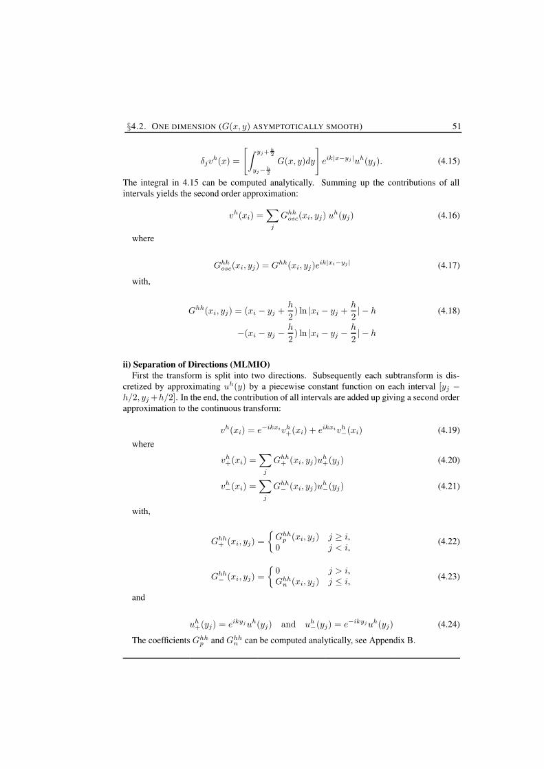
§4.2. ONE DIMENSION (G(x, y) ASYMPTOTICALLY SMOOTH) 51
δjvh(x) =
[
∫ yj+h2
yj−h2
G(x, y)dy
]
eik|x−yj |uh(yj). (4.15)
The integral in 4.15 can be computed analytically. Summing up the contributions of allintervals yields the second order approximation:
vh(xi) =∑
j
Ghhosc(xi, yj) uh(yj) (4.16)
where
Ghhosc(xi, yj) = Ghh(xi, yj)e
ik|xi−yj | (4.17)
with,
Ghh(xi, yj) = (xi − yj +h
2) ln |xi − yj +
h
2| − h (4.18)
−(xi − yj −h
2) ln |xi − yj −
h
2| − h
ii) Separation of Directions (MLMIO)First the transform is split into two directions. Subsequently each subtransform is dis-
cretized by approximating uh(y) by a piecewise constant function on each interval [yj −h/2, yj +h/2]. In the end, the contribution of all intervals are added up giving a second orderapproximation to the continuous transform:
vh(xi) = e−ikxivh+(xi) + eikxivh
−(xi) (4.19)
where
vh+(xi) =
∑
j
Ghh+ (xi, yj)u
h+(yj) (4.20)
vh−(xi) =
∑
j
Ghh− (xi, yj)u
h−(yj) (4.21)
with,
Ghh+ (xi, yj) =
Ghhp (xi, yj) j ≥ i,
0 j < i,(4.22)
Ghh− (xi, yj) =
0 j > i,Ghh
n (xi, yj) j ≤ i, (4.23)
and
uh+(yj) = eikyj uh(yj) and uh
−(yj) = e−ikyj uh(yj) (4.24)
The coefficients Ghhp and Ghh
n can be computed analytically, see Appendix B.

52 CHAPTER 4. NUMERICAL RESULTS MLMIO
4.2.2 PerformanceThe results for this model problem will be presented in a same way as for the previous prob-lem. First the dependence of the accuracy on the mesh size and the wave number (k = 64πfor this case) is given in the third column (cl = fl) of the table 4.6, which actually is thediscretization error. Next, the results for the MLMIO algorithm are presented in the tables4.6 and 4.7 and Figures 4.5, 4.6 and 4.7. Additional results are given in the Appendix B.
Since in both cases, single matrix multiplication and separation of directions, the functionu is approximated by a piecewise constant and the coefficients G, G+ and G− are evaluatedanalytically, there is no difference between the results obtained on a single grid with the twoapproaches.
In table 4.6 and B.7 and B.10 the discretization error (column cl = fl) is defined as:
||ε||2 =1
n + 1
n∑
i=0
|v(xi) − vh(xi)| (4.25)
which is given as a function of the mesh size for the cases with k = 8π, 32π and 64πrespectively. From the results it can be seen that the discretization error is indeed O(h2) asexpected.
||ε||, k = 64πfl Mesh cl=fl cl=fl-1 cl=fl-2 cl=fl-3 cl=fl-4 cl=fl-58 512 2.36e-03 2.36e-03 2.36e-03 2.36e-03 2.36e-03 2.36e-039 1024 6.18e-04 6.18e-04 6.18e-04 6.18e-04 6.18e-04 6.18e-04*
10 2048 1.62e-04 1.62e-04 1.62e-04 1.62e-04 1.62e-04 1.62e-0411 4096 4.23e-05 4.23e-05 4.23e-05 4.23e-05 4.22e-05 4.23e-0512 8192 1.10e-05 1.10e-05 1.10e-05 1.10e-05 1.10e-05 1.10e-0513 16384 2.87e-06 2.87e-06 2.87e-06 2.88e-06 2.88e-06 2.87e-0614 32768 7.47e-07 7.47e-07 7.47e-07 7.48e-07 7.49e-07 7.49e-0715 65536 1.94e-07 1.94e-07 1.94e-07 1.94e-07 1.95e-07 1.96e-0716 131072 5.03e-08 5.03e-08 5.03e-08 5.03e-08 5.05e-08 5.10e-0817 262144 1.30e-08 1.30e-08 1.30e-08 1.30e-08 1.31e-08 1.31e-08
TABLE 4.6: Average norm of the error in the numerical evaluation of (4.13) using the MLMIOalgorithm with p = 8 order transfers. (k = 64π)
To illustrate the performance of the MLMIO algorithm the fast evaluation error will beused which is defined as:
||FEε||2 =1
n + 1
n∑
i=0
|vh(xi)fl − vh(xi)
cl| (4.26)
i.e. the difference between the result obtained on the target grid using no coarse grids at alland the results obtained on the target grid using the MLMIO algorithm in which the actualsummation take place on grid cl.
In the fast evaluation, as a result of the singularity a local correction is needed for the errormade by the interpolation near the singularity, see section 3.2.3. In this case a correction wasintroduced for the contribution of m = 3 + ln(n) points around (xi = yj).
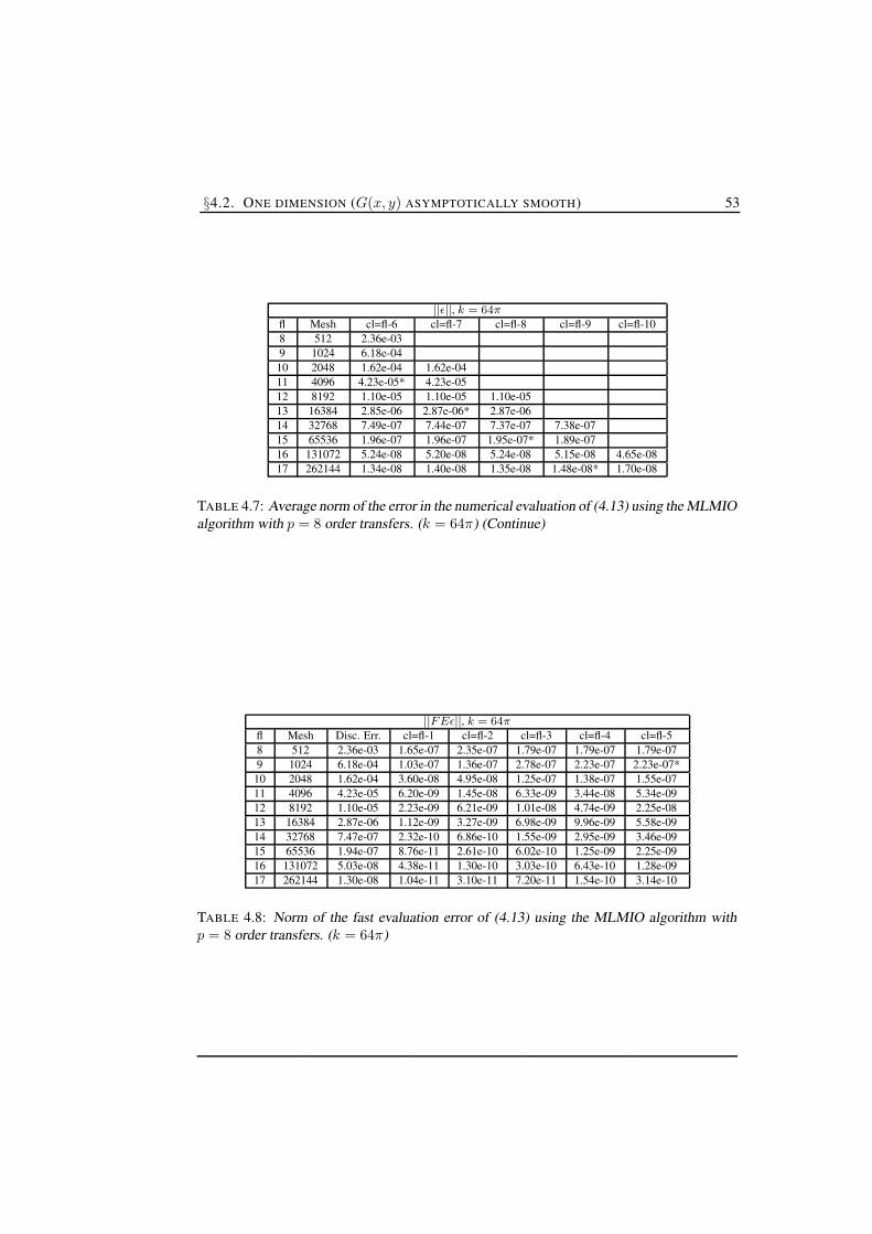
§4.2. ONE DIMENSION (G(x, y) ASYMPTOTICALLY SMOOTH) 53
||ε||, k = 64πfl Mesh cl=fl-6 cl=fl-7 cl=fl-8 cl=fl-9 cl=fl-108 512 2.36e-039 1024 6.18e-0410 2048 1.62e-04 1.62e-0411 4096 4.23e-05* 4.23e-0512 8192 1.10e-05 1.10e-05 1.10e-0513 16384 2.85e-06 2.87e-06* 2.87e-0614 32768 7.49e-07 7.44e-07 7.37e-07 7.38e-0715 65536 1.96e-07 1.96e-07 1.95e-07* 1.89e-0716 131072 5.24e-08 5.20e-08 5.24e-08 5.15e-08 4.65e-0817 262144 1.34e-08 1.40e-08 1.35e-08 1.48e-08* 1.70e-08
TABLE 4.7: Average norm of the error in the numerical evaluation of (4.13) using the MLMIOalgorithm with p = 8 order transfers. (k = 64π) (Continue)
||FEε||, k = 64πfl Mesh Disc. Err. cl=fl-1 cl=fl-2 cl=fl-3 cl=fl-4 cl=fl-58 512 2.36e-03 1.65e-07 2.35e-07 1.79e-07 1.79e-07 1.79e-079 1024 6.18e-04 1.03e-07 1.36e-07 2.78e-07 2.23e-07 2.23e-07*10 2048 1.62e-04 3.60e-08 4.95e-08 1.25e-07 1.38e-07 1.55e-0711 4096 4.23e-05 6.20e-09 1.45e-08 6.33e-09 3.44e-08 5.34e-0912 8192 1.10e-05 2.23e-09 6.21e-09 1.01e-08 4.74e-09 2.25e-0813 16384 2.87e-06 1.12e-09 3.27e-09 6.98e-09 9.96e-09 5.58e-0914 32768 7.47e-07 2.32e-10 6.86e-10 1.55e-09 2.95e-09 3.46e-0915 65536 1.94e-07 8.76e-11 2.61e-10 6.02e-10 1.25e-09 2.25e-0916 131072 5.03e-08 4.38e-11 1.30e-10 3.03e-10 6.43e-10 1.28e-0917 262144 1.30e-08 1.04e-11 3.10e-11 7.20e-11 1.54e-10 3.14e-10
TABLE 4.8: Norm of the fast evaluation error of (4.13) using the MLMIO algorithm withp = 8 order transfers. (k = 64π)
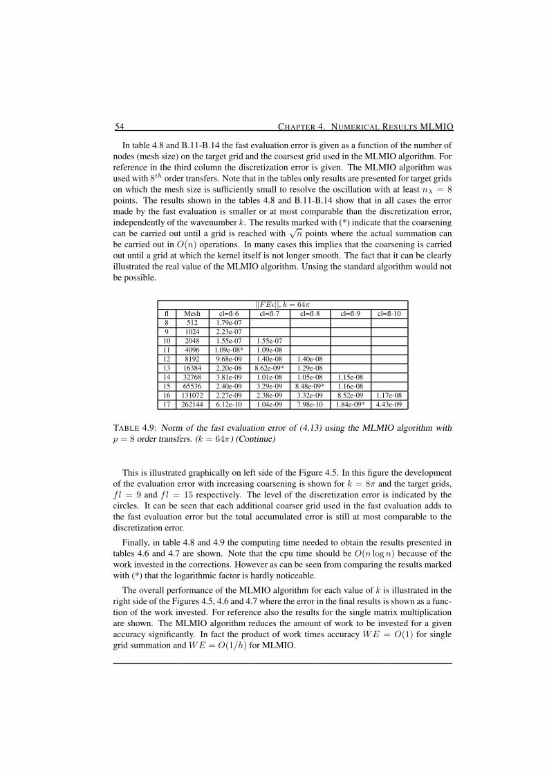
54 CHAPTER 4. NUMERICAL RESULTS MLMIO
In table 4.8 and B.11-B.14 the fast evaluation error is given as a function of the number ofnodes (mesh size) on the target grid and the coarsest grid used in the MLMIO algorithm. Forreference in the third column the discretization error is given. The MLMIO algorithm wasused with 8th order transfers. Note that in the tables only results are presented for target gridson which the mesh size is sufficiently small to resolve the oscillation with at least nλ = 8points. The results shown in the tables 4.8 and B.11-B.14 show that in all cases the errormade by the fast evaluation is smaller or at most comparable than the discretization error,independently of the wavenumber k. The results marked with (*) indicate that the coarseningcan be carried out until a grid is reached with
√n points where the actual summation can
be carried out in O(n) operations. In many cases this implies that the coarsening is carriedout until a grid at which the kernel itself is not longer smooth. The fact that it can be clearlyillustrated the real value of the MLMIO algorithm. Unsing the standard algorithm would notbe possible.
||FEε||, k = 64πfl Mesh cl=fl-6 cl=fl-7 cl=fl-8 cl=fl-9 cl=fl-108 512 1.79e-079 1024 2.23e-0710 2048 1.55e-07 1.55e-0711 4096 1.09e-08* 1.09e-0812 8192 9.68e-09 1.40e-08 1.40e-0813 16384 2.20e-08 8.62e-09* 1.29e-0814 32768 3.81e-09 1.01e-08 1.05e-08 1.15e-0815 65536 2.40e-09 3.29e-09 8.48e-09* 1.16e-0816 131072 2.27e-09 2.38e-09 3.32e-09 8.52e-09 1.17e-0817 262144 6.12e-10 1.04e-09 7.98e-10 1.84e-09* 4.43e-09
TABLE 4.9: Norm of the fast evaluation error of (4.13) using the MLMIO algorithm withp = 8 order transfers. (k = 64π) (Continue)
This is illustrated graphically on left side of the Figure 4.5. In this figure the developmentof the evaluation error with increasing coarsening is shown for k = 8π and the target grids,fl = 9 and fl = 15 respectively. The level of the discretization error is indicated by thecircles. It can be seen that each additional coarser grid used in the fast evaluation adds tothe fast evaluation error but the total accumulated error is still at most comparable to thediscretization error.
Finally, in table 4.8 and 4.9 the computing time needed to obtain the results presented intables 4.6 and 4.7 are shown. Note that the cpu time should be O(n log n) because of thework invested in the corrections. However as can be seen from comparing the results markedwith (*) that the logarithmic factor is hardly noticeable.
The overall performance of the MLMIO algorithm for each value of k is illustrated in theright side of the Figures 4.5, 4.6 and 4.7 where the error in the final results is shown as a func-tion of the work invested. For reference also the results for the single matrix multiplicationare shown. The MLMIO algorithm reduces the amount of work to be invested for a givenaccuracy significantly. In fact the product of work times accuracy WE = O(1) for singlegrid summation and WE = O(1/h) for MLMIO.
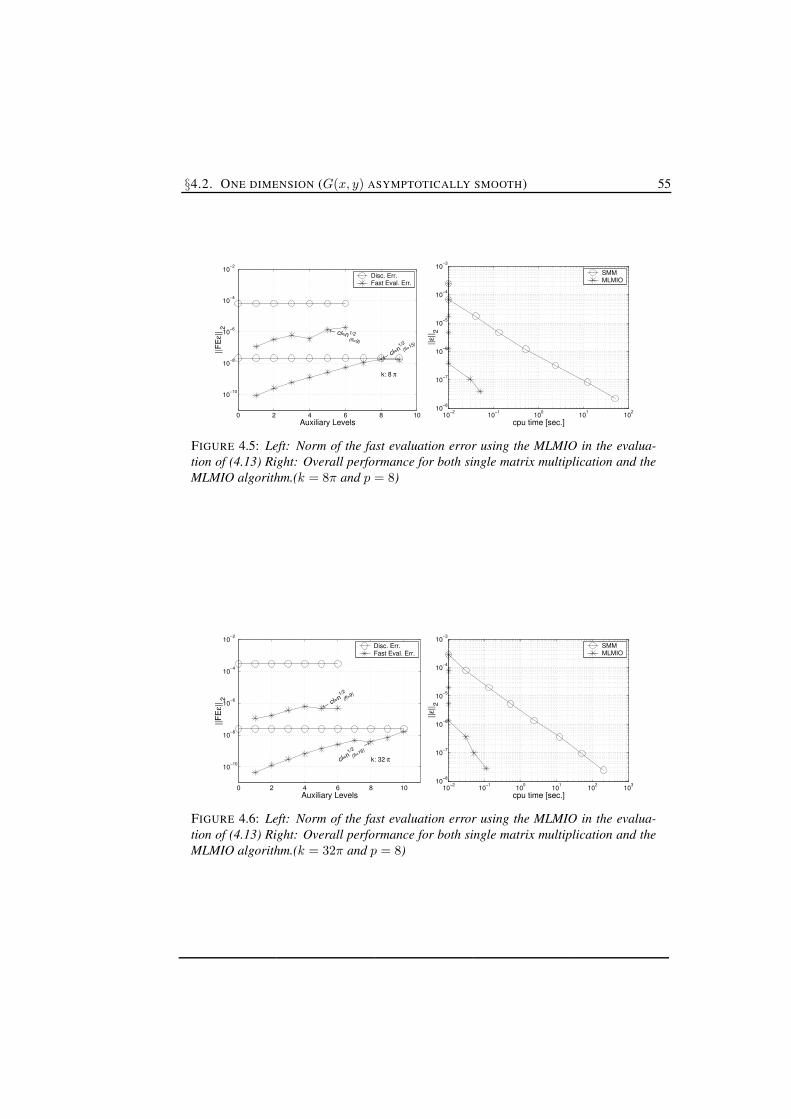
§4.2. ONE DIMENSION (G(x, y) ASYMPTOTICALLY SMOOTH) 55
0 2 4 6 8 10
10−10
10−8
10−6
10−4
10−2
Auxiliary Levels
||FE
ε|| 2
k: 8 π
← cl=n 1/2 (fl=9)
← cl=n1/2
(fl=15)
Disc. Err.Fast Eval. Err.
10−2
10−1
100
101
102
10−8
10−7
10−6
10−5
10−4
10−3
cpu time [sec.]||ε
|| 2
SMMMLMIO
FIGURE 4.5: Left: Norm of the fast evaluation error using the MLMIO in the evalua-tion of (4.13) Right: Overall performance for both single matrix multiplication and theMLMIO algorithm.(k = 8π and p = 8)
0 2 4 6 8 10
10−10
10−8
10−6
10−4
10−2
Auxiliary Levels
||FE
ε|| 2
k: 32 π
← cl=n1/2
(fl=9)
cl=n1/2
(fl=16)
→
Disc. Err.Fast Eval. Err.
10−2
10−1
100
101
102
103
10−8
10−7
10−6
10−5
10−4
10−3
cpu time [sec.]
||ε|| 2
SMMMLMIO
FIGURE 4.6: Left: Norm of the fast evaluation error using the MLMIO in the evalua-tion of (4.13) Right: Overall performance for both single matrix multiplication and theMLMIO algorithm.(k = 32π and p = 8)

56 CHAPTER 4. NUMERICAL RESULTS MLMIO
0 2 4 6 8 1010
−12
10−10
10−8
10−6
10−4
10−2
Auxiliary Levels
||FE
ε|| 2
k: 64 π
← cl=n1/2
(fl=9)
← cl=n 1/2 (fl=17)
Disc. Err.Fast Eval. Err.
10−2
10−1
100
101
102
103
10−8
10−7
10−6
10−5
10−4
10−3
cpu time [sec.]
||ε|| 2
SMMMLMIO
FIGURE 4.7: Left: Norm of the fast evaluation error using the MLMIO in the evalua-tion of (4.13) Right: Overall performance for both single matrix multiplication and theMLMIO algorithm.(k = 64π and p = 8)
4.3 Two dimensional problem: G(x, y) explicit oscillatoryIn the one dimensional case the separation of directions isolates the effect of the oscillatorybehaviour of the kernel into functions of x and y that can be taken outside the integral andincorporated in the u(y) respectively. As a result the algorithm for oscillatory kernels differsonly little from the regular algorithm. The required computational effort for the fast evalua-tion of a discrete integral transform with an oscillatory kernel is only twice the effort neededthat is needed for an asymptotically smooth kernel. The real test is off course the two di-mensional case where the algorithm is much more involved as the separation of directions isimplicit, and the number of directions increases each additional coarsening step.
The first two dimensional model problem considered is the evaluation of an integral trans-form with asymptotically smooth explicit oscillatory kernel. The total kernel is exactly of theform assumed in the generic problem used to describe the algorithm in chapter 3.
The general notation introduced in section 3.1 is used with d = 2 and d = d, x andy ∈ IR2, so that x = (x1, x2) and y = (y1, y2) with |x − y| = [(x1 − y1)2 + (x2 − y2)2]
1
2 .The model problem is defined as the evaluation of:
v(x) =
∫
Ω
G(x, y) eik|x−y| u(y) dy, x ∈ Ω (4.27)
with Ω ∈ [−1, 1] × [−1, 1], where
G(x, y) =1
|x − y| (4.28)
and
u(y) ≡ u(y1, y2) = sin(ky1) sin(ky2), y ∈ Ω (4.29)
for different values of k. Note that for this problem the wavenumber k is introduced also inthe function u(y) with the aim to represent modal behaviour as is often the case in practical

§4.3. TWO DIMENSIONAL PROBLEM: G(x, y) EXPLICIT OSCILLATORY 57
applications. However, note that the behaviour or u(y) plays no role at all in the algorithm. Infact, a more oscillatory u(y) makes fast evaluation easier. This is because the discretizationerror for an oscillatory u(y) is larger so the permissible error in the fast evaluation algorithmis larger and lower order transfers are already sufficient to achieve the result.
4.3.1 DiscretizationAs for the one dimensional model problems the performance of the MLMIO algorithm isillustrated by comparing results for two cases.
The notation below is as defined in section 3.1, so that yj ∈ IR2 (i.e. yj = (y1j , y2
j )) is apoint of the integration grid and at this location the value of u(yj) is assumed to be given.The integral transform v(x) is to be evaluated in all points xi ∈ IR2 (i.e. xi = (x1
i , x2i )) of
an evaluation grid is the location of a receiver point v(xi). The distance between two pointsxi and yj is |xi − yj | = [(x1
i − y1j )2 + (x2
i − y2j )2]
1
2 .
i) Single Matrix MultiplicationThe product eik|x−y|u(y) is approximated by a piecewise constant function on each inte-
gration interval of size h×h centered around of the point yj . Subsequently the contribution ofeach interval is computed. Summing up over all integration intervals then yields the followingsecond order approximation to (4.27):
vh(xi) =∑
j
Ghhosc(xi, yj) uh(yj) (4.30)
where
Ghhosc(xi, yj) = Ghh(xi, yj) eik|xi−yj | (4.31)
with
Ghh(xi, yj) ≡ Ghh(x1i , x
2i , y
1j , y2
j ) =
∫ y1
j + h2
y1
j−h
2
∫ y2
j + h2
y2
j−h
2
dy1dy2
[(x1i − y1)2 + (x2
i − y2)2]1
2
(4.32)
and
uh(yj) ≡ uh(y1j , y2
j ) = sin(ky1j ) sin(ky2
j ) (4.33)
The integrals in (4.32) can be evaluated analytically, see Appendix B. Note that for an uniformgrid these coefficients only depend on the distance between the point xi and yj and can beprecomputed and stored in O(n) operations.
ii) Separation of Directions (MLMIO)The second formulation is obtained using the description given in Section 3.3 in terms of
separation of directions. The approximation to (4.27) is:
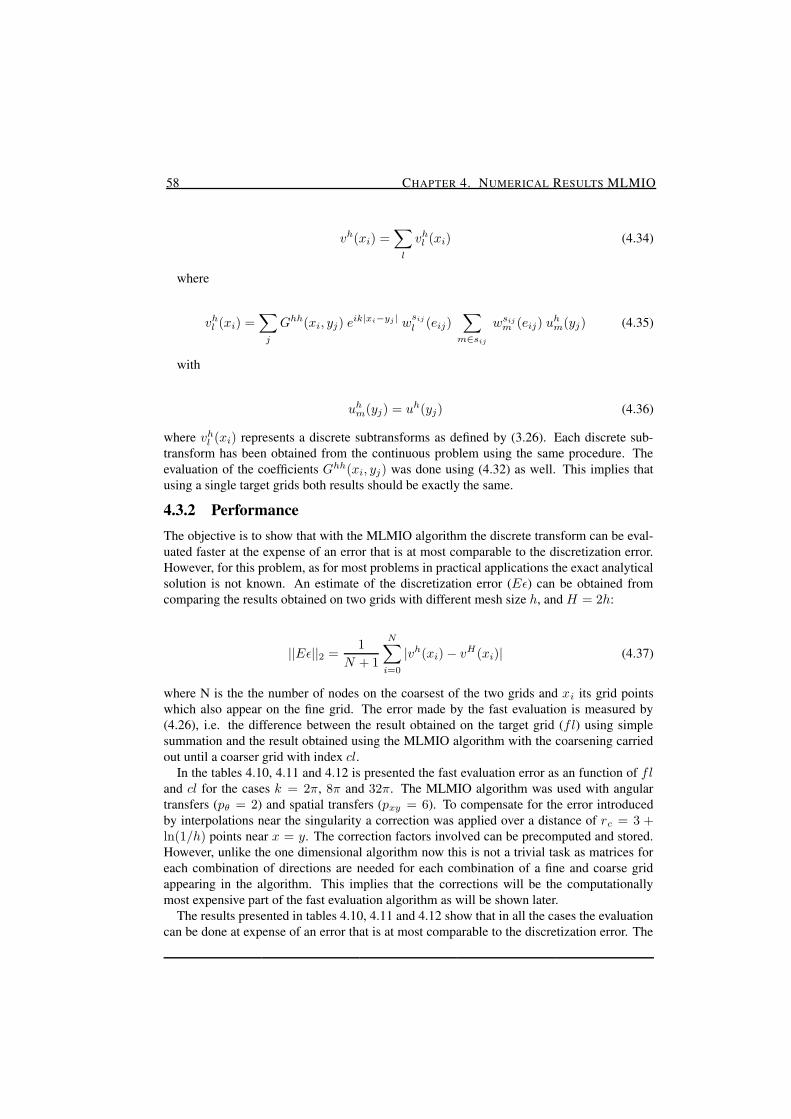
58 CHAPTER 4. NUMERICAL RESULTS MLMIO
vh(xi) =∑
l
vhl (xi) (4.34)
where
vhl (xi) =
∑
j
Ghh(xi, yj) eik|xi−yj | wsij
l (eij)∑
m∈sij
wsijm (eij) uh
m(yj) (4.35)
with
uhm(yj) = uh(yj) (4.36)
where vhl (xi) represents a discrete subtransforms as defined by (3.26). Each discrete sub-
transform has been obtained from the continuous problem using the same procedure. Theevaluation of the coefficients Ghh(xi, yj) was done using (4.32) as well. This implies thatusing a single target grids both results should be exactly the same.
4.3.2 PerformanceThe objective is to show that with the MLMIO algorithm the discrete transform can be eval-uated faster at the expense of an error that is at most comparable to the discretization error.However, for this problem, as for most problems in practical applications the exact analyticalsolution is not known. An estimate of the discretization error (Eε) can be obtained fromcomparing the results obtained on two grids with different mesh size h, and H = 2h:
||Eε||2 =1
N + 1
N∑
i=0
|vh(xi) − vH(xi)| (4.37)
where N is the the number of nodes on the coarsest of the two grids and xi its grid pointswhich also appear on the fine grid. The error made by the fast evaluation is measured by(4.26), i.e. the difference between the result obtained on the target grid (fl) using simplesummation and the result obtained using the MLMIO algorithm with the coarsening carriedout until a coarser grid with index cl.
In the tables 4.10, 4.11 and 4.12 is presented the fast evaluation error as an function of fland cl for the cases k = 2π, 8π and 32π. The MLMIO algorithm was used with angulartransfers (pθ = 2) and spatial transfers (pxy = 6). To compensate for the error introducedby interpolations near the singularity a correction was applied over a distance of rc = 3 +ln(1/h) points near x = y. The correction factors involved can be precomputed and stored.However, unlike the one dimensional algorithm now this is not a trivial task as matrices foreach combination of directions are needed for each combination of a fine and coarse gridappearing in the algorithm. This implies that the corrections will be the computationallymost expensive part of the fast evaluation algorithm as will be shown later.
The results presented in tables 4.10, 4.11 and 4.12 show that in all the cases the evaluationcan be done at expense of an error that is at most comparable to the discretization error. The
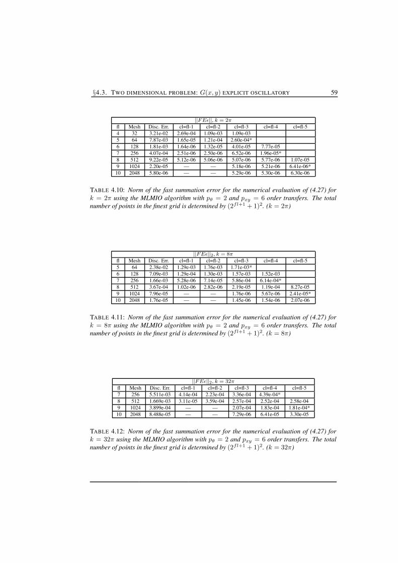
§4.3. TWO DIMENSIONAL PROBLEM: G(x, y) EXPLICIT OSCILLATORY 59
||FEε||, k = 2πfl Mesh Disc. Err. cl=fl-1 cl=fl-2 cl=fl-3 cl=fl-4 cl=fl-54 32 3.21e-02 2.69e-04 1.09e-03 1.09e-035 64 7.87e-03 1.65e-05 1.21e-04 2.60e-04*6 128 1.81e-03 1.64e-06 1.32e-05 4.01e-05 7.77e-057 256 4.07e-04 2.51e-06 2.50e-06 6.52e-06 1.96e-05*8 512 9.22e-05 5.12e-06 5.06e-06 5.07e-06 5.77e-06 1.07e-059 1024 2.20e-05 — — 5.18e-06 5.21e-06 6.41e-06*10 2048 5.80e-06 — — 5.29e-06 5.30e-06 6.30e-06
TABLE 4.10: Norm of the fast summation error for the numerical evaluation of (4.27) fork = 2π using the MLMIO algorithm with pθ = 2 and pxy = 6 order transfers. The totalnumber of points in the finest grid is determined by (2fl+1 + 1)2. (k = 2π)
||FEε||2 , k = 8πfl Mesh Disc. Err. cl=fl-1 cl=fl-2 cl=fl-3 cl=fl-4 cl=fl-55 64 2.38e-02 1.29e-03 1.76e-03 1.71e-03*6 128 7.09e-03 1.29e-04 1.30e-03 1.57e-03 1.52e-037 256 1.66e-03 5.28e-06 7.14e-05 5.86e-04 6.14e-04*8 512 3.67e-04 1.02e-06 2.82e-06 2.19e-05 1.19e-04 8.27e-059 1024 7.96e-05 — — 1.76e-06 5.67e-06 2.41e-05*10 2048 1.76e-05 — — 1.45e-06 1.54e-06 2.07e-06
TABLE 4.11: Norm of the fast summation error for the numerical evaluation of (4.27) fork = 8π using the MLMIO algorithm with pθ = 2 and pxy = 6 order transfers. The totalnumber of points in the finest grid is determined by (2fl+1 + 1)2. (k = 8π)
||FEε||2, k = 32πfl Mesh Disc. Err. cl=fl-1 cl=fl-2 cl=fl-3 cl=fl-4 cl=fl-57 256 5.511e-03 4.14e-04 2.23e-04 3.36e-04 4.39e-04*8 512 1.669e-03 3.11e-05 3.59e-04 2.57e-04 2.52e-04 2.58e-049 1024 3.899e-04 — — 2.07e-04 1.83e-04 1.81e-04*10 2048 8.488e-05 — — 7.29e-06 6.41e-05 3.30e-05
TABLE 4.12: Norm of the fast summation error for the numerical evaluation of (4.27) fork = 32π using the MLMIO algorithm with pθ = 2 and pxy = 6 order transfers. The totalnumber of points in the finest grid is determined by (2fl+1 + 1)2. (k = 32π)
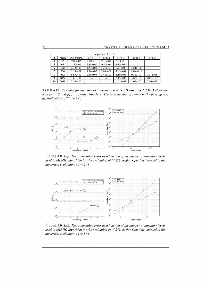
60 CHAPTER 4. NUMERICAL RESULTS MLMIO
Cpu time, k = 2πfl Mesh Dir. Summ. cl=fl-1 cl=fl-2 cl=fl-3 cl=fl-4 cl=fl-54 32 2.00e-02 2.80e-01 2.10e-01 2.30e-015 64 1.50e-01 1.84e+00 9.40e-01 9.60e-01*6 128 2.32e+00 1.51e+01 4.21e+00 3.71e+00 3.84e+007 256 5.19e+01 1.76e+02 2.90e+01 1.85e+01 1.89e+01*8 512 8.65e+02 2.38e+03 2.44e+02 1.10e+02 9.58e+01 9.94e+019 1024 1.61e+04 — — 5.13e+02 3.88e+02 3.88e+02*
10 2048 2.54e+05 — — 4.01e+03 2.09e+03 2.00e+03
TABLE 4.13: Cpu time for the numerical evaluation of (4.27) using the MLMIO algorithmwith pθ = 2 and pxy = 6 order transfers. The total number of points in the finest grid isdetermined by (2fl+1 + 1)2.
0 1 2 3 4 5 6 710
−6
10−5
10−4
10−3
10−2
10−1
Auxiliary Levels
||FE
ε|| 2
k: 2 π ← cl=n1/2
(fl=5)
← cl=n1/2
(fl=9)
Disc. Err. (Estimated)Fast Eval. Err.
101
102
103
10−2
10−1
100
101
102
103
104
105
106
n per edge
cpu
time
[sec
.]SMMMLMIO
FIGURE 4.8: Left: Fast summation error as a function of the number of auxiliary levelsused in MLMIO algorithm for the evaluation of (4.27). Right: Cpu time invested in thenumerical evaluation. (k = 2π)
0 1 2 3 4 5 6 710
−6
10−5
10−4
10−3
10−2
Auxiliary Levels
||FE
ε|| 2
k: 8 π ← cl=n1/2 (fl=5)
← cl=n1/2 (fl=9)
Disc. Err. (Estimated)Fast Eval. Err.
102
103
10−1
100
101
102
103
104
105
106
n per edge
cpu
time
[sec
.]
SMMMLMIO
FIGURE 4.9: Left: Fast summation error as a function of the number of auxiliary levelsused in MLMIO algorithm for the evaluation of (4.27). Right: Cpu time invested in thenumerical evaluation. (k = 8π)
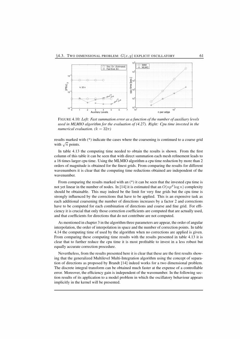
§4.3. TWO DIMENSIONAL PROBLEM: G(x, y) EXPLICIT OSCILLATORY 61
0 1 2 3 4 5 6 710
−4
10−3
10−2
Auxiliary Levels
||FE
ε|| 2
k: 32 π
← cl=n1/2 (fl=6)
← cl=n1/2
(fl=9)
Disc. Err. (Estimated)Fast Eval. Err.
102
103
101
102
103
104
105
106
n per edge
cpu
time
[sec
.]
SMMMLMIO
FIGURE 4.10: Left: Fast summation error as a function of the number of auxiliary levelsused in MLMIO algorithm for the evaluation of (4.27). Right: Cpu time invested in thenumerical evaluation. (k = 32π)
results marked with (*) indicate the cases where the coarsening is continued to a coarse gridwith
√n points.
In table 4.13 the computing time needed to obtain the results is shown. From the firstcolumn of this table it can be seen that with direct summation each mesh refinement leads toa 16 times larger cpu time. Using the MLMIO algorithm a cpu time reduction by more than 2orders of magnitude is obtained for the finest grids. From comparing the results for differentwavenumbers it is clear that the computing time reductions obtained are independent of thewavenumber.
From comparing the results marked with an (*) it can be seen that the invested cpu time isnot yet linear in the number of nodes. In [14] it is estimated that an O(npd log n) complexityshould be obtainable. This may indeed be the limit for very fine grids but the cpu time isstrongly influenced by the corrections that have to be applied. This is an expensive task aseach additional coarsening the number of directions increases by a factor 2 and correctionshave to be computed for each combination of directions and coarse and fine grid. For effi-ciency it is crucial that only those correction coefficients are computed that are actually used,and that coefficients for directions that do not contribute are not computed.
As mentioned in chapter 3 in the algorithm three parameters are appear, the order of angularinterpolation, the order of interpolation in space and the number of correction points. In table4.14 the computing time of used by the algorithm when no corrections are applied is given.From comparing these computing time results with the results presented in table 4.13 it isclear that to further reduce the cpu time it is most profitable to invest in a less robust butequally accurate correction procedure.
Nevertheless, from the results presented here it is clear that these are the first results show-ing that the generalized Multilevel Multi-Integration algorithm using the concept of separa-tion of directions as proposed by Brandt [14] indeed works for a two dimensional problem.The discrete integral transform can be obtained much faster at the expense of a controllableerror. Moreover, the efficiency gain is independent of the wavenumber. In the following sec-tion results of its application to a model problem in which the oscillatory behaviour appearsimplicitly in the kernel will be presented.
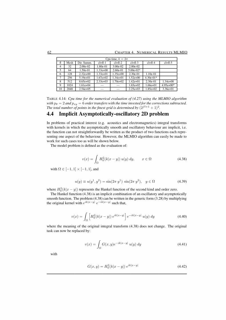
62 CHAPTER 4. NUMERICAL RESULTS MLMIO
Cpu time, k = 2πfl Mesh Dir. Summ. cl=fl-1 cl=fl-2 cl=fl-3 cl=fl-4 cl=fl-54 32 2.00e-02 1.80e-01 3.00e-02 2.00e-025 64 1.50e-01 1.33e+00 2.60e-01 5.00e-02*6 128 2.32e+00 1.33e+01 1.35e+00 2.30e-01 1.10e-017 256 5.19e+01 1.67e+02 1.34e+01 1.52e+00 4.30e-01*8 512 8.65e+02 2.33e+03 1.70e+02 1.42e+01 2.30e-01 1.34e+009 1024 1.61e+04 — — 1.65e+02 1.66e+01 4.95e+00*10 2048 2.54e+05 — — 2.25e+03 1.85e+02 3.36e+01
TABLE 4.14: Cpu time for the numerical evaluation of (4.27) using the MLMIO algorithmwith pθ = 2 and pxy = 6 order transfers with the time invested for the corrections subtracted.The total number of points in the finest grid is determined by (2fl+1 + 1)2.
4.4 Implicit Asymptotically-oscillatory 2D problemIn problems of practical interest (e.g. acoustics and electromagnetics) integral transformswith kernels in which the asymptotically smooth and oscillatory behaviour are implicit, i.e.the function can not straightforwardly be written as the product of two functions each repre-senting one aspect of the behaviour. However, the MLMIO algorithm can easily be made towork for such cases too as will be shown below.
The model problem is defined as the evaluation of:
v(x) =
∫
Ω
H20 (k|x − y|) u(y) dy, x ∈ Ω (4.38)
with Ω ∈ [−1, 1] × [−1, 1], and
u(y) ≡ u(y1, y2) = sin(2π y1) sin(2π y2), y ∈ Ω (4.39)
where H20 (k|x − y|) represents the Hankel function of the second kind and order zero.
The Hankel function (4.38) is an implicit combination of an oscillatory and asymptoticallysmooth function. The problem (4.38) can be written in the generic form (3.28) by multiplyingthe original kernel with eik|x−y| e−ik|x−y| such that,
v(x) =
∫
Ω
[
H20 (k|x − y|) eik|x−y|
]
e−ik|x−y| u(y) dy (4.40)
where the meaning of the original integral transform (4.38) does not change. The originaltask can now be replaced by:
v(x) =
∫
Ω
G(x, y)e−ik|x−y| u(y) dy (4.41)
with
G(x, y) = H20 (k|x − y|) eik|x−y| (4.42)
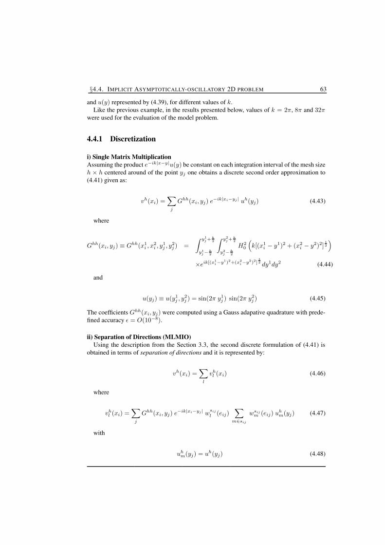
§4.4. IMPLICIT ASYMPTOTICALLY-OSCILLATORY 2D PROBLEM 63
and u(y) represented by (4.39), for different values of k.Like the previous example, in the results presented below, values of k = 2π, 8π and 32π
were used for the evaluation of the model problem.
4.4.1 Discretization
i) Single Matrix MultiplicationAssuming the product e−ik|x−y|u(y) be constant on each integration interval of the mesh sizeh × h centered around of the point yj one obtains a discrete second order approximation to(4.41) given as:
vh(xi) =∑
j
Ghh(xi, yj) e−ik|xi−yj | uh(yj) (4.43)
where
Ghh(xi, yj) ≡ Ghh(x1i , x
2i , y
1j , y2
j ) =
∫ y1
j + h2
y1
j−h2
∫ y2
j + h2
y2
j−h2
H20
(
k[(x1i − y1)2 + (x2
i − y2)2]1
2
)
×eik[(x1
i−y1)2+(x2
i−y2)2]1
2 dy1dy2 (4.44)
and
u(yj) ≡ u(y1j , y2
j ) = sin(2π y1j ) sin(2π y2
j ) (4.45)
The coefficients Ghh(xi, yj) were computed using a Gauss adapative quadrature with prede-fined accuracy ε = O(10−8).
ii) Separation of Directions (MLMIO)Using the description from the Section 3.3, the second discrete formulation of (4.41) is
obtained in terms of separation of directions and it is represented by:
vh(xi) =∑
l
vhl (xi) (4.46)
where
vhl (xi) =
∑
j
Ghh(xi, yj) e−ik|xi−yj | wsij
l (eij)∑
m∈sij
wsijm (eij) uh
m(yj) (4.47)
with
uhm(yj) = uh(yj) (4.48)

64 CHAPTER 4. NUMERICAL RESULTS MLMIO
where vhl (xi) represents each of the subtransforms defined by (3.37). Note that because the
kernel of the original integral transform (4.38) was replaced by an explicit product of the bothasymptotically smooth and oscillatory functions the evaluation of the coefficients Ghh(xi, yj)can now be done using (4.44).
4.4.2 PerformanceThe performance is illustrated in the same way as for the previous example. As the exactanalytical solution is not known the fast evaluation error defined by (4.26) is compared withthe estimate of the discretization error as defined by (4.37). As a reminder, the fast evaluationerror is the difference between the result obtained on the target grid (fl) using simple sum-mation and the result obtained on this grid using the MLMIO algorithm with the coarseningcarried out until a coarser grid with index cl.
In the tables 4.15, 4.16 and 4.17 the fast evaluation error is presented as a function of fland cl for the case k = 2π, 8π and 32π. The MLMIO algorithm was used with angulartransfers (pθ = 2) and spatial transfers (pxy = 6). The correction was carried out over aregion of rc = 3 + ln(1/h) points around the singularity at x = y.
Tables 4.15, 4.16 and 4.17 show the fast evaluation error ontained with the MLMIO algo-rithm, where for all the cases the error is at most comparable to the discretization error. Theresults marked with (*) indicate the cases where the coarsest auxiliary grid reached has
√n
points.
||FEε||2 , k = 2πfl Mesh Disc. Err. cl=fl-1 cl=fl-2 cl=fl-3 cl=fl-4 cl=fl-54 32 3.085e-03 8.70e-05 4.16e-04 4.16e-045 64 7.017e-04 3.87e-06 3.94e-05 9.96e-05*6 128 1.658e-04 2.54e-07 2.69e-06 1.14e-05 2.76e-057 256 4.053e-05 4.19e-07 4.11e-07 1.27e-06 5.24e-06*8 512 1.009e-05 8.95e-07 8.56e-07 8.56e-07 1.05e-06 2.74e-069 1024 2.669e-06 — — 8.57e-07 8.61e-07 1.05e-06*10 2048 7.276e-07 — — — 8.94e-07 9.01e-07
TABLE 4.15: Norm of the fast summation error for 2D problem with Hankel function askernel. The total number of points on the finest grid is determined by (2fl+1 +1)2. (MLMIO,k = 2π)
||FEε||2 , k = 8πfl Mesh Disc. Err. cl=fl-1 cl=fl-2 cl=fl-3 cl=fl-4 cl=fl-55 64 5.906e-04 2.60e-05 6.88e-05 9.55e-05*6 128 9.683e-05 7.12e-07 5.90e-06 3.91e-05 6.77e-057 256 1.692e-05 5.67e-08 1.05e-07 4.21e-06 1.11e-05*8 512 3.512e-06 4.05e-08 6.86e-08 9.77e-08 5.47e-07 1.12e-059 1024 8.434e-07 — — 4.67e-08 7.15e-08 7.40e-07*10 2048 2.156e-07 — — — 2.64e-08 5.26e-08
TABLE 4.16: Norm of the fast summation error for 2D problem with Hankel function askernel. The total number of points on the finest grid is determined by (2fl+1 +1)2. (MLMIO,k = 8π)
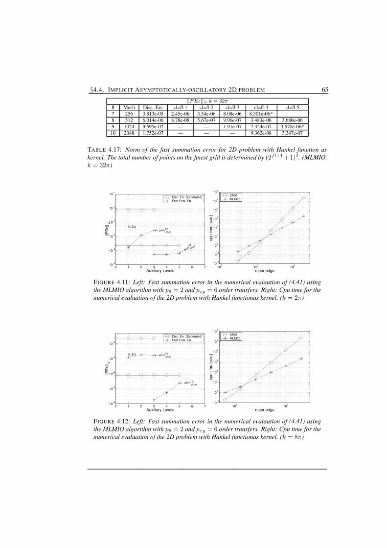
§4.4. IMPLICIT ASYMPTOTICALLY-OSCILLATORY 2D PROBLEM 65
||FEε||2, k = 32πfl Mesh Disc. Err. cl=fl-1 cl=fl-2 cl=fl-3 cl=fl-4 cl=fl-57 256 3.813e-05 2.45e-06 3.54e-06 8.08e-06 8.301e-06*8 512 6.014e-06 8.78e-08 5.67e-07 9.96e-07 3.483e-06 3.680e-069 1024 9.695e-07 — — 1.91e-07 7.324e-07 3.670e-06*10 2048 1.752e-07 — — — 9.362e-08 3.347e-07
TABLE 4.17: Norm of the fast summation error for 2D problem with Hankel function askernel. The total number of points on the finest grid is determined by (2fl+1 +1)2. (MLMIO,k = 32π)
0 1 2 3 4 5 6 710
−6
10−5
10−4
10−3
10−2
10−1
Auxiliary Levels
||FE
ε|| 2
k: 2 π ← cl=n1/2
(fl=5)
← cl=n1/2
(fl=9)
Disc. Err. (Estimated)Fast Eval. Err.
101
102
103
10−2
10−1
100
101
102
103
104
105
106
n per edge
cpu
time
[sec
.]
SMMMLMIO
FIGURE 4.11: Left: Fast summation error in the numerical evalaution of (4.41) usingthe MLMIO algorithm with pθ = 2 and pxy = 6 order transfers. Right: Cpu time for thenumerical evaluation of the 2D problem with Hankel functionas kernel. (k = 2π)
0 1 2 3 4 5 6 710
−6
10−5
10−4
10−3
10−2
Auxiliary Levels
||FE
ε|| 2
k: 8 π ← cl=n1/2 (fl=5)
← cl=n1/2 (fl=9)
Disc. Err. (Estimated)Fast Eval. Err.
102
103
10−1
100
101
102
103
104
105
106
n per edge
cpu
time
[sec
.]
SMMMLMIO
FIGURE 4.12: Left: Fast summation error in the numerical evalaution of (4.41) usingthe MLMIO algorithm with pθ = 2 and pxy = 6 order transfers. Right: Cpu time for thenumerical evaluation of the 2D problem with Hankel functionas kernel. (k = 8π)
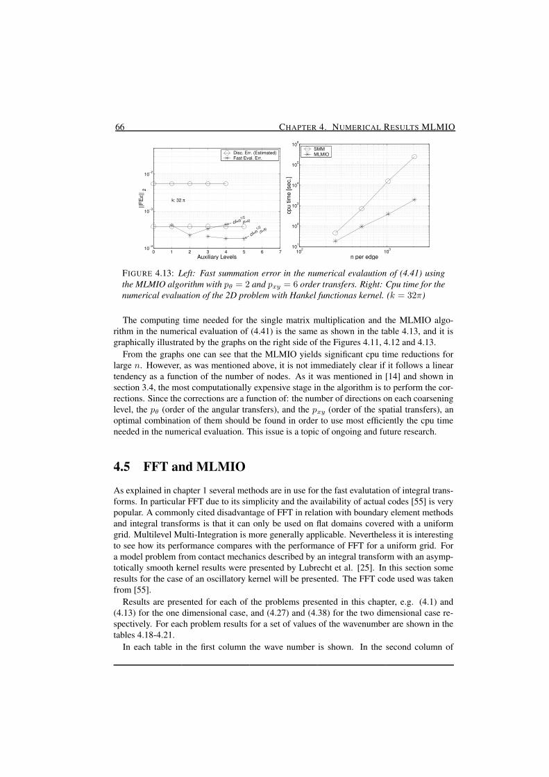
66 CHAPTER 4. NUMERICAL RESULTS MLMIO
0 1 2 3 4 5 6 710
−4
10−3
10−2
Auxiliary Levels
||FE
ε|| 2
k: 32 π
← cl=n1/2 (fl=6)
← cl=n1/2
(fl=9)
Disc. Err. (Estimated)Fast Eval. Err.
102
103
101
102
103
104
105
106
n per edge
cpu
time
[sec
.]
SMMMLMIO
FIGURE 4.13: Left: Fast summation error in the numerical evalaution of (4.41) usingthe MLMIO algorithm with pθ = 2 and pxy = 6 order transfers. Right: Cpu time for thenumerical evaluation of the 2D problem with Hankel functionas kernel. (k = 32π)
The computing time needed for the single matrix multiplication and the MLMIO algo-rithm in the numerical evaluation of (4.41) is the same as shown in the table 4.13, and it isgraphically illustrated by the graphs on the right side of the Figures 4.11, 4.12 and 4.13.
From the graphs one can see that the MLMIO yields significant cpu time reductions forlarge n. However, as was mentioned above, it is not immediately clear if it follows a lineartendency as a function of the number of nodes. As it was mentioned in [14] and shown insection 3.4, the most computationally expensive stage in the algorithm is to perform the cor-rections. Since the corrections are a function of: the number of directions on each coarseninglevel, the pθ (order of the angular transfers), and the pxy (order of the spatial transfers), anoptimal combination of them should be found in order to use most efficiently the cpu timeneeded in the numerical evaluation. This issue is a topic of ongoing and future research.
4.5 FFT and MLMIO
As explained in chapter 1 several methods are in use for the fast evalutation of integral trans-forms. In particular FFT due to its simplicity and the availability of actual codes [55] is verypopular. A commonly cited disadvantage of FFT in relation with boundary element methodsand integral transforms is that it can only be used on flat domains covered with a uniformgrid. Multilevel Multi-Integration is more generally applicable. Nevertheless it is interestingto see how its performance compares with the performance of FFT for a uniform grid. Fora model problem from contact mechanics described by an integral transform with an asymp-totically smooth kernel results were presented by Lubrecht et al. [25]. In this section someresults for the case of an oscillatory kernel will be presented. The FFT code used was takenfrom [55].
Results are presented for each of the problems presented in this chapter, e.g. (4.1) and(4.13) for the one dimensional case, and (4.27) and (4.38) for the two dimensional case re-spectively. For each problem results for a set of values of the wavenumber are shown in thetables 4.18-4.21.
In each table in the first column the wave number is shown. In the second column of
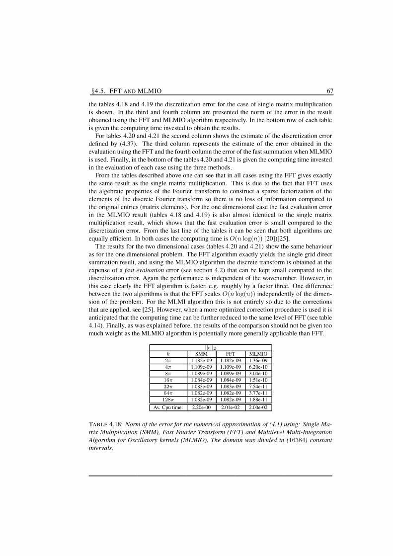
§4.5. FFT AND MLMIO 67
the tables 4.18 and 4.19 the discretization error for the case of single matrix multiplicationis shown. In the third and fourth column are presented the norm of the error in the resultobtained using the FFT and MLMIO algorithm respectively. In the bottom row of each tableis given the computing time invested to obtain the results.
For tables 4.20 and 4.21 the second column shows the estimate of the discretization errordefined by (4.37). The third column represents the estimate of the error obtained in theevaluation using the FFT and the fourth column the error of the fast summation when MLMIOis used. Finally, in the bottom of the tables 4.20 and 4.21 is given the computing time investedin the evaluation of each case using the three methods.
From the tables described above one can see that in all cases using the FFT gives exactlythe same result as the single matrix multiplication. This is due to the fact that FFT usesthe algebraic properties of the Fourier transform to construct a sparse factorization of theelements of the discrete Fourier transform so there is no loss of information compared tothe original entries (matrix elements). For the one dimensional case the fast evaluation errorin the MLMIO result (tables 4.18 and 4.19) is also almost identical to the single matrixmultiplication result, which shows that the fast evaluation error is small compared to thediscretization error. From the last line of the tables it can be seen that both algorithms areequally efficient. In both cases the computing time is O(n log(n)) [20])[25].
The results for the two dimensional cases (tables 4.20 and 4.21) show the same behaviouras for the one dimensional problem. The FFT algorithm exactly yields the single grid directsummation result, and using the MLMIO algorithm the discrete transform is obtained at theexpense of a fast evaluation error (see section 4.2) that can be kept small compared to thediscretization error. Again the performance is independent of the wavenumber. However, inthis case clearly the FFT algorithm is faster, e.g. roughly by a factor three. One differencebetween the two algorithms is that the FFT scales O(n log(n)) independently of the dimen-sion of the problem. For the MLMI algorithm this is not entirely so due to the correctionsthat are applied, see [25]. However, when a more optimized correction procedure is used it isanticipated that the computing time can be further reduced to the same level of FFT (see table4.14). Finally, as was explained before, the results of the comparison should not be given toomuch weight as the MLMIO algorithm is potentially more generally applicable than FFT.
||ε||2k SMM FFT MLMIO2π 1.182e-09 1.182e-09 1.36e-094π 1.109e-09 1.109e-09 6.20e-108π 1.089e-09 1.089e-09 3.04e-1016π 1.084e-09 1.084e-09 1.51e-1032π 1.083e-09 1.083e-09 7.54e-1164π 1.082e-09 1.082e-09 3.77e-11128π 1.082e-09 1.082e-09 1.88e-11
Av. Cpu time: 2.20e-00 2.01e-02 2.00e-02
TABLE 4.18: Norm of the error for the numerical approximation of (4.1) using: Single Ma-trix Multiplication (SMM), Fast Fourier Transform (FFT) and Multilevel Multi-IntegrationAlgorithm for Oscillatory kernels (MLMIO). The domain was divided in (16384) constantintervals.
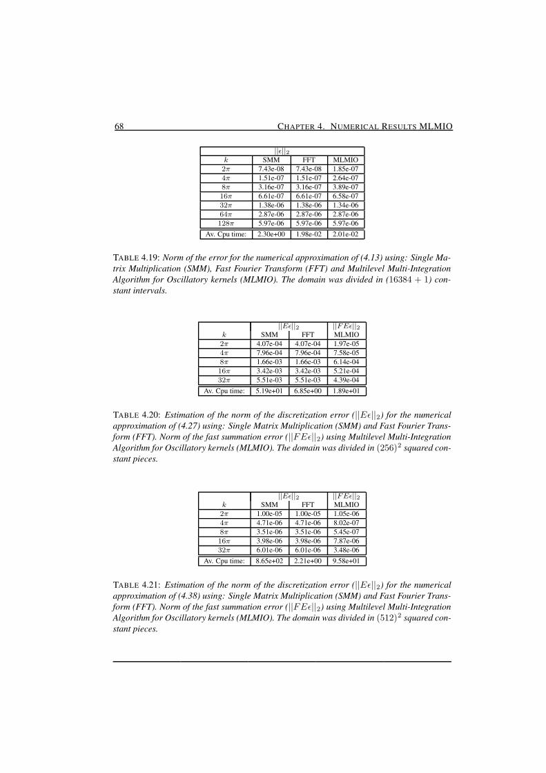
68 CHAPTER 4. NUMERICAL RESULTS MLMIO
||ε||2k SMM FFT MLMIO2π 7.43e-08 7.43e-08 1.85e-074π 1.51e-07 1.51e-07 2.64e-078π 3.16e-07 3.16e-07 3.89e-0716π 6.61e-07 6.61e-07 6.58e-0732π 1.38e-06 1.38e-06 1.34e-0664π 2.87e-06 2.87e-06 2.87e-06128π 5.97e-06 5.97e-06 5.97e-06
Av. Cpu time: 2.30e+00 1.98e-02 2.01e-02
TABLE 4.19: Norm of the error for the numerical approximation of (4.13) using: Single Ma-trix Multiplication (SMM), Fast Fourier Transform (FFT) and Multilevel Multi-IntegrationAlgorithm for Oscillatory kernels (MLMIO). The domain was divided in (16384 + 1) con-stant intervals.
||Eε||2 ||FEε||2k SMM FFT MLMIO2π 4.07e-04 4.07e-04 1.97e-054π 7.96e-04 7.96e-04 7.58e-058π 1.66e-03 1.66e-03 6.14e-0416π 3.42e-03 3.42e-03 5.21e-0432π 5.51e-03 5.51e-03 4.39e-04
Av. Cpu time: 5.19e+01 6.85e+00 1.89e+01
TABLE 4.20: Estimation of the norm of the discretization error (||Eε||2) for the numericalapproximation of (4.27) using: Single Matrix Multiplication (SMM) and Fast Fourier Trans-form (FFT). Norm of the fast summation error (||FEε||2) using Multilevel Multi-IntegrationAlgorithm for Oscillatory kernels (MLMIO). The domain was divided in (256)2 squared con-stant pieces.
||Eε||2 ||FEε||2k SMM FFT MLMIO2π 1.00e-05 1.00e-05 1.05e-064π 4.71e-06 4.71e-06 8.02e-078π 3.51e-06 3.51e-06 5.45e-0716π 3.98e-06 3.98e-06 7.87e-0632π 6.01e-06 6.01e-06 3.48e-06
Av. Cpu time: 8.65e+02 2.21e+00 9.58e+01
TABLE 4.21: Estimation of the norm of the discretization error (||Eε||2) for the numericalapproximation of (4.38) using: Single Matrix Multiplication (SMM) and Fast Fourier Trans-form (FFT). Norm of the fast summation error (||FEε||2) using Multilevel Multi-IntegrationAlgorithm for Oscillatory kernels (MLMIO). The domain was divided in (512)2 squared con-stant pieces.
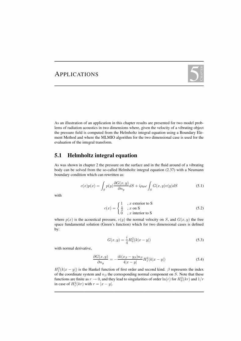
5 CH
AP
TE
R
APPLICATIONS
As an illustration of an application in this chapter results are presented for two model prob-lems of radiation acoustics in two dimensions where, given the velocity of a vibrating objectthe pressure field is computed from the Helmholtz integral equation using a Boundary Ele-ment Method and where the MLMIO algorithm for the two dimensional case is used for theevaluation of the integral transform.
5.1 Helmholtz integral equationAs was shown in chapter 2 the pressure on the surface and in the fluid around of a vibratingbody can be solved from the so-called Helmholtz integral equation (2.37) with a Neumannboundary condition which can rewritten as:
c(x)p(x) =
∫
S
p(y)∂G(x, y)
∂nydS + ıρ0ω
∫
S
G(x, y)v(y)dS (5.1)
with
c(x) =
1 , x exterior to S12 , x on S0 , x interior to S
(5.2)
where p(x) is the acoustical pressure, v(y) the normal velocity on S, and G(x, y) the freespace fundamental solution (Green’s function) which for two dimensional cases is definedby:
G(x, y) =i
4H2
0 (k|x − y|) (5.3)
with normal derivative,
∂G(x, y)
∂ny= − ik(xβ − yβ)nβ
4|x − y| H21 (k|x − y|) (5.4)
H21 (k|x − y|) is the Hankel function of first order and second kind. β represents the index
of the coordinate system and nβ the corresponding normal component on S. Note that thesefunctions are finite as r → 0, and they lead to singularities of order ln(r) for H2
0 (kr) and 1/rin case of H2
1 (kr) with r = |x − y|.
70 CHAPTER 5. APPLICATIONS
In section 2.3 it was mentioned that in order to solve p in the domain two steps are required:
1. Solve the equation for pressure p(x) on the surface using,
c(x)p(x)−∫
S
p(y)∂G(x, y)
∂nydS = ıρ0ω
∫
S
G(x, y)v(y)dS (5.5)
2. Given the pressure p(y) on the surface, evaluate the pressure p(x) at any location inthe field using (5.1).
As was shown by Schenck[62] solving the surface Helmholtz integral equation non-uniquenessproblems of the solution have to be overcome related to the natural frequencies of the asso-ciated interior Dirichlet problem. Several methods have been proposed to overcome theseproblems:The Combined Helmholtz Integral Equation Formulation (CHIEF)
Schenck [62] proposes to remove the nonuniquense by introducing additional Helmholtz in-tegral relations evaluated in the interior of the domain. Applying a discretization of the ra-diating surface to the CHIEF equations leads to an over determined system of the equationsfor the surface pressure which can be solved in the last squares sense. However, a potentialcomplication of this method is the choice of the interior points at which the supplementalequations are defined such that to any possible distortion of the solution due to the interiorcritical frequencies is avoided.
The hypersingular formulation
This method was introduced by Burton and Miller [21] and has been widely studied. Themethod is based in the generation of an integral equation valid for all wavenumbers by form-ing a linear combination of the Helmholtz integral relations used by CHIEF and its normalderivative. However, a complication in this approach is the evaluation of the hyper-singularintegrals involving a double normal derivative of the free space Green’s function. Most re-cently efforts to improve the approach have been investigated developing efficient methodsto evaluate the hyper singular integrals, see [5].Visser [74] proposes a combination of the CHIEF and the hyper-singular formulation, refer-ring to it as Combined Interior Burton-Miller Formulation (CIBMF).
In the cases shown in this chapter the CHIEF method was used.
5.2 Direct BEM discretizationThe Boundary Element Method is a most suitable numerical approach for the evaluation ofexterior acoustical problems using the direct formulation of the Helmholtz integral equation(5.1), e.g. see [22].
In the direct BEM method, the first step is to derive from the continuous equation a discretesystem of equations from which the unknowns at specific points at the boundary can besolved. The boundary of the body is divided into N segments where the variables p (pressure)and v (normal velocity) are approximated on the surface by locally based functions p(y) andv(y) defined on each surface element (panel).
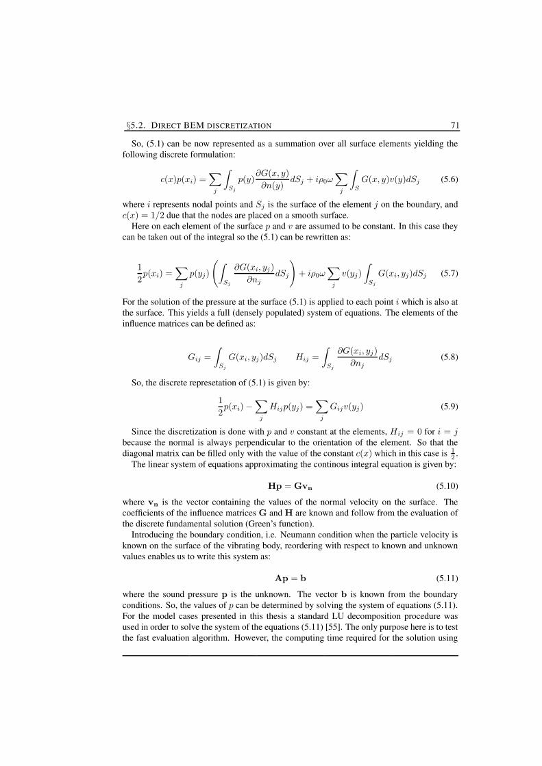
§5.2. DIRECT BEM DISCRETIZATION 71
So, (5.1) can be now represented as a summation over all surface elements yielding thefollowing discrete formulation:
c(x)p(xi) =∑
j
∫
Sj
p(y)∂G(x, y)
∂n(y)dSj + iρ0ω
∑
j
∫
S
G(x, y)v(y)dSj (5.6)
where i represents nodal points and Sj is the surface of the element j on the boundary, andc(x) = 1/2 due that the nodes are placed on a smooth surface.
Here on each element of the surface p and v are assumed to be constant. In this case theycan be taken out of the integral so the (5.1) can be rewritten as:
1
2p(xi) =
∑
j
p(yj)
(
∫
Sj
∂G(xi, yj)
∂njdSj
)
+ iρ0ω∑
j
v(yj)
∫
Sj
G(xi, yj)dSj (5.7)
For the solution of the pressure at the surface (5.1) is applied to each point i which is also atthe surface. This yields a full (densely populated) system of equations. The elements of theinfluence matrices can be defined as:
Gij =
∫
Sj
G(xi, yj)dSj Hij =
∫
Sj
∂G(xi, yj)
∂njdSj (5.8)
So, the discrete represetation of (5.1) is given by:
1
2p(xi) −
∑
j
Hijp(yj) =∑
j
Gijv(yj) (5.9)
Since the discretization is done with p and v constant at the elements, Hij = 0 for i = jbecause the normal is always perpendicular to the orientation of the element. So that thediagonal matrix can be filled only with the value of the constant c(x) which in this case is 1
2 .The linear system of equations approximating the continous integral equation is given by:
Hp = Gvn (5.10)
where vn is the vector containing the values of the normal velocity on the surface. Thecoefficients of the influence matrices G and H are known and follow from the evaluation ofthe discrete fundamental solution (Green’s function).
Introducing the boundary condition, i.e. Neumann condition when the particle velocity isknown on the surface of the vibrating body, reordering with respect to known and unknownvalues enables us to write this system as:
Ap = b (5.11)
where the sound pressure p is the unknown. The vector b is known from the boundaryconditions. So, the values of p can be determined by solving the system of equations (5.11).For the model cases presented in this thesis a standard LU decomposition procedure wasused in order to solve the system of the equations (5.11) [55]. The only purpose here is to testthe fast evaluation algorithm. However, the computing time required for the solution using
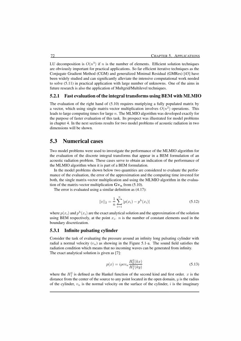
72 CHAPTER 5. APPLICATIONS
LU decomposition is O(n3) if n is the number of elements. Efficient solution techniquesare obviously important for practical applications. So far efficient iterative techniques as theConjugate Gradient Method (CGM) and generalized Minimal Residual (GMRes) [43] havebeen widely studied and can significantly alleviate the intensive computational work neededto solve (5.11) in practical application with large number of unknowns. One of the aims infuture research is also the application of Multgrid/Multilevel techniques.
5.2.1 Fast evaluation of the integral transforms using BEM with MLMIOThe evaluation of the right hand of (5.10) requires mutiplying a fully populated matrix bya vector, which using single matrix-vector multiplication involves O(n2) operations. Thisleads to large computing times for large n. The MLMIO algorithm was developed exactly forthe purpose of faster evaluation of this task. Its prospect was illustrated for model problemsin chapter 4. In the next sections results for two model problems of acoustic radiation in twodimensions will be shown.
5.3 Numerical casesTwo model problems were used to investigate the performance of the MLMIO algorithm forthe evaluation of the discrete integral transforms that appear in a BEM formulation of anacoustic radiation problem. These cases serve to obtain an indication of the performance ofthe MLMIO algorithm when it is part of a BEM formulation.
In the model problems shown below two quantities are considered to evaluate the perfor-mance of the evaluation, the error of the approximation and the computing time invested forboth, the single matrix-vector multiplication and using the MLMIO algorithm in the evalua-tion of the matrix-vector multiplication Gvn from (5.10).
The error is evaluated using a similar definition as (4.17):
||ε||2 =1
n
n∑
i=1
|p(xi) − ph(xi)| (5.12)
where p(xi) and ph(xi) are the exact analytical solution and the approximation of the solutionusing BEM respectively, at the point xi. n is the number of constant elements used in theboundary discretization.
5.3.1 Infinite pulsating cylinderConsider the task of evaluating the pressure around an infinity long pulsating cylinder withradial a normal velocity (vn) as showing in the Figure 5.1-a. The sound field satisfies theradiation condition which means that no incoming waves can be generated from infinity.The exact analytical solution is given as [7]:
p(x) = iρcvnH2
0 (kx)
H21 (ky)
(5.13)
where the H21 is defined as the Hankel function of the second kind and first order. x is the
distance from the center of the source to any point located in the open domain, y is the radiusof the cylinder, vn is the normal velocity on the surface of the cylinder, i is the imaginary
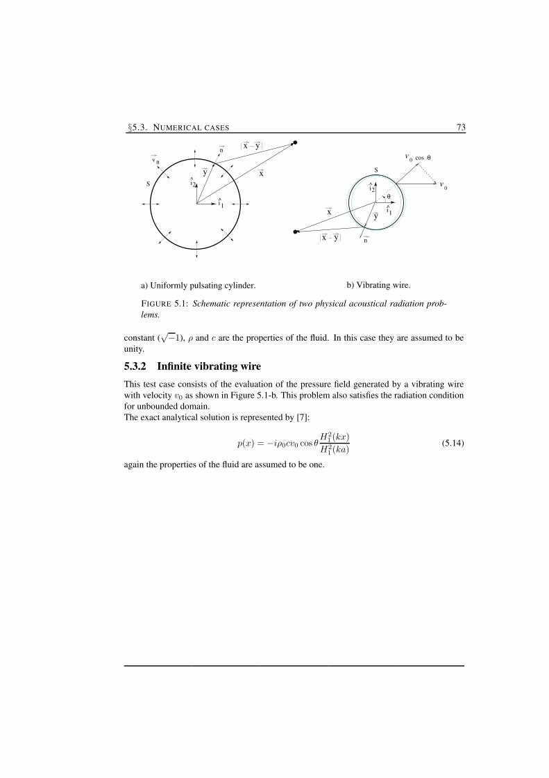
§5.3. NUMERICAL CASES 73
yx
x 1i
^
θ
S
b) Vibrating wire.a) Uniformly pulsating cylinder.
S2
xy
i
nvn
yx
1
cos
i
y
θ
n
^2i
0v
0v
FIGURE 5.1: Schematic representation of two physical acoustical radiation prob-lems.
constant (√−1), ρ and c are the properties of the fluid. In this case they are assumed to be
unity.
5.3.2 Infinite vibrating wireThis test case consists of the evaluation of the pressure field generated by a vibrating wirewith velocity v0 as shown in Figure 5.1-b. This problem also satisfies the radiation conditionfor unbounded domain.The exact analytical solution is represented by [7]:
p(x) = −iρ0cv0 cos θH2
1 (kx)
H21 (ka)
(5.14)
again the properties of the fluid are assumed to be one.

74 CHAPTER 5. APPLICATIONS

6 CH
AP
TE
RCONCLUSIONS AND
RECOMMENDATIONS
6.1 Conclusion
A low noise level is a strategic quality for products ranging from personal appliances to aero-planes. Reliable and efficient methods and computational tools to design silent products andto identify sources of noise are urgently needed. Impressive results have been obtained withmodels and computer simulations to predict noise for specific problems. However, it is still along way towards efficient and reliable computational tools for the design of silent productsin many practical applications. A crucial bottleneck is that the required computational effortis often far too large for extensive use of the computer simulations in design.
In this thesis an alternative algorithm for the fast numerical evaluation of integral trans-forms with oscillatory Green’s functions as they appear in acoustic radiation problems hasbeen developed. The algorithm is the generalization of the Multilevel Multi-Integration algo-rithm which was introduced and proven to be very efficient for transforms with smooth andasymptotically smooth Green’s functions by Brandt and Lubrecht [16]. In the generalizedalgorithm, using the concept of separation of directions and the smoothness of the oscillatorypart as a function of the phase angle the original transform is rewritten as a special case of themore generalized task of the evaluation of a series of transforms each with an asymptoticallysmooth Green’s function. The smoothness of these functions can then be used to replace theoriginal task on the target grid by a series of intergrid transfers and a coarse grid discretetransform. This concept was outlined by Brandt [14] over a decade ago but no numericalresults were presented so far. In this thesis it has been demonstrated that the concept reallyworks. A careful step by step approach was adopted starting with one dimensional modelproblems for which the concept is straightforward. Subsequently, the much more involvedtwo dimensional problem was tackled. Also for this case results were presented for trans-forms with different Green’s functions including the Hankel function which appears in manypractical applications. It has been shown that the algorithm yields an accurate approximationto the discrete integral transform with an error that can be kept comparable to the discretiza-tion error that is made anyway, in a computing time that is much smaller. The performanceis independent of the wavenumber which is crucial as in practice the computing time prob-lems are most urgent for high frequencies where large numbers of nodes are required. Therequired cpu time is reduced from O(n2) to O(npd log n) operations. So far only uniformgrids were used. The algorithm was benchmarked against the popular Fast Fourier Transformwhich also has a O(n log n) complexity but is restricted to uniform grids on flat domains. For
76 CHAPTER 6. CONCLUSIONS AND RECOMMENDATIONS
the two dimensional problem the required cpu time is about three times larger than used byan FFT algorithm. However, the main goal of this thesis was to prove that the concept worksand yields a fast alternative algorithm. Optimization of the computation of the a posterioricorrections will most certainly lead to an algorithm that for uniform grids is fully competitivewith FFT. Besides, the uniform grid case is only for testing. The algorithm has the prospectthat it can be used for non-uniform grids and grids on curved surfaces.
As a first step towards implementation in Boundary Element Methods for acoustic radiationproblems in chapter 5 some first results obtained with a BEM algorithm obtained for someaccoustic model problems were presented.
6.2 Recommandations for further research
The evaluation of integral transforms with oscillatory kernels using the multilevel multi-integration algorithm involves the following tasks: coarsening (spatial anterpolation and an-gular interpolation), fast summation (multisummation on the coarsest level), refining (spatialinterpolation and angular anterpolation), and correction (involving directions, angular andspatial interpolations).
As was shown in the chapters three and four the computationally most expensive task inthe algorithm is the computation of the a posteriori corrections related to the error introducedin the region around the singularity where the auxiliary kernels are not smooth. A detailedoptimization of the different parameters in the algorithm ,i.e. the angular interpolation (pθ),the spatial interpolation (pxy) and the size of the correction rc, e.g. by carrying out an opti-mization analysis as done in [16] and [17] can be carried out to further optimize the algorithmand to reduce the size of the correction region. Also, in the present implementation the cor-rection matrices are computed by applying the algorithm itself in a local form. The advantageof this approach is that it is very robust as it allows correction for any approximation made inthe algorithm, including some of the assumptions of angular smoothness of variables in thecoarsening procedure. It thus allows correction to zero error which is important in a develop-ment stage. However, various cheaper alternatives should be investigated such as correctionbased on the spatial interpolation error in the auxiliary kernels only or the use alternative ofkernel softening around the singularity. This will lead to further reductions of computingtime and the use of memory involved in storing the correction coefficients.
Another option for further development is the following. In the algorithm as describedin chapter 3 the spatial coarsening is the same for each direction y1 and y2 (or x1 and x2).However, as can be seen from the auxiliary kernels Gijlm(x, y) for a given l this kernelis much smoother in the direction m on the grid than in the direction perpendicular to m.Hence, when represented on a grid aligned with this direction it can be represented with thesame accuracy using a larger meshsize in the direction of alignment. The idea is now tointroduce spatial grids aligned with the different directions on the angular grid. Subsequentlyin the coarsening these grids can be coarsened faster in the direction of alignment than in thecross direction. As a result the total number of nodes on the all coarser grids will decreasefaster than 2d−1 which can lead to an even more efficient algorithm. A similar approachhas proven successful in the development of a multigrid solver for the Helmholtz equation indifferential form developed, see [15].
However, before exploiting such possibilities it is important that the present algorithm finds
§6.2. RECOMMANDATIONS FOR FURTHER RESEARCH 77
its way towards applications to help alleviate computing time problems. In this respect it isimportant that the extension to three dimensional problems is implemented first as well as theextension to curved surfaces.
As shown in chapter 5 the evaluation of the integral transform is usually a subtask in theprocess of solving the integral equation. In principle the algorithm presented here can alreadybe used for this purpose in combination with any type of solver. However, as has been shownin research in contact mechanics and lubrication problems there is an enormous prospect ofefficiency increase when also for the solution of the integral equation multigrid techniquesare used, see [70]. Multigrid techniques provide many options to further reduce the computa-tional effort in acoustic radiation problems also for the inverse problem where complicationsarising from regularization may be overcome by appropriate use of the different scales. Inthis respect the research presented in this thesis is a crucial first step.

78 CHAPTER 6. CONCLUSIONS AND RECOMMENDATIONS
REFERENCES
[1] M. Abramowitz and I.A. Segun, Handbook of mathematical functions, Dover Publica-tions, Inc., New-York, USA, 1968.
[2] S. Amini and S.M. Kirkup, Solution of the Helmholtz equation in the exterior domain byelementary boundary integral methods, Journal of Computational Physics, 118 (1995)208-221.
[3] L. Baker, C mathematical function handbook, McGraw-Hill, USA, 1992.
[4] G.K. Batchelor, An introduction to fluid dynamics, Cambridge University Press, NewYork, USA, 2000.
[5] W. Benthien and A. Schenck, Nonexistence and nonuniqueness problems associatedwith integral equation methods in acoustics, Computers and Structures, 65 (1997) 295-305.
[6] R.B. Bird, W.E. Stewart, and E.N. Lightfoot, Transport Phenomena, John Wiley andSons, New York, USA, 1960.
[7] D.T. Blackstock, Fundamentals of physical acoustics, John Wiley and Sons, New York,USA, 2000.
[8] J. Barnes and P. Hut, A hierarchical O(N log N) force-calculation algorithm, Nature,324 (1986) 446-449.
[9] A. Boag, E. Michielssen, and A. Brandt, Nonuniform polar grid algorithm for fast fieldevaluation, IEEE Antennas and Wireless Propagation Letters, 1 (2002) 142-145.
[10] A. Boag, A fast multilevel domain decomposition algorithm for radar imaging, IEEETransaction on Antennas and Propagation, 49 (2001) 666-671
[11] A. Boag, A fast iterative physical optics (FIPO) algorithm based on non-uniform polargrid interpolation, Microwave and Optical Technology Letters, 35 (2002) 240-244.
[12] J. Board and K. Schulten, The fast multipole algorithm, Computing in Science andEngineering, 2 (2000) 76-79.
[13] J. Bos, Frictional heating of tribological contacts, University of Twente, PhD thesis,Enschede, The Netherlands, 1995.
80 REFERENCES
[14] A. Brandt, Multilevel computations of integral transforms and particle interactions withoscillatory kernels, Computer Physics Communications, 65 (1991) 24-38.
[15] A. Brandt and I. Livshits, Wave-ray multigrid method for standing wave equations,Electronic Transactions on Numerical Analysis, 6 (1997) 162-181.
[16] A. Brandt and A.A. Lubrecht, Multilevel matrix multiplication and fast solution of in-tegral equations, Journal of Compuational Physics, 90 (1990) 348-370.
[17] A. Brandt and C.H. Venner, Multilevel evaluation of integral transforms with asymptot-ically smooth kernels, SIAM Journal on Scientific Computing, 19 (1998) 468-492.
[18] A. Brandt and C.H. Venner, Multilevel evaluation of integral transforms on adaptivegrids, Gauss Center Report WI/GC-5, Rehovot, Israel, 1996.
[19] W.L. Briggs, V.E. Henson, and S.F. McCormick, A multigrid tutorial, SIAM, Philadel-phia, USA, 2000.
[20] E.O. Brigham, The fast Fourier transform and its applications, Prentice Hall, New Jer-sey, USA, 1988.
[21] A.J. Burton and G.F. Miller, The application of integral equation methods to the nu-merical solution of some exterior boundary-value problems, Proceedings of the RoyalSociety of London. Serie A, Mathematical and Physical Sciences, 323 (1971) 201-210.
[22] R.D. Ciskowski and C.A. Brebbia, Boundary element method in acoustics, Wessex In-stitue of Technology, Southapton, UK, 1990.
[23] R. Coifman, V. Rokhlin, and S. Wandzura, The fast multipole method for the waveequation: A Pedestrian Prescription, IEEE Antennas and Propagation, 35 (1993) 7-12.
[24] J.W. Cooley and J.W. Tukey, An algorithm for the machine computation of complexFourier series, Mathematics of Computations, 19 (1965) 297-301.
[25] F. Colin and A.A. Lubrecht, Comparison of FFT-MLMI for elastic deformation calcu-lations, Journal of Tribology, ASME, 123 (2001) 884-887.
[26] G. Dahlquist and A. Bjorck, Numerical methods, Printice Hall, New Jersey, USA, 2001.
[27] E. Darve, Methodes multipoles rapides: resolution des equations de Maxwell par for-mulations integrales, l’Univerite Paris 6, these de Doctorat, Paris, France, 1999.
[28] E. Darve, The fast multipole method: numerical implementation, Journal of Computa-tional Physics, 160 (2000) 195-240.
[29] H.E. de Bree, The Microflown, ISBN 90-365-1579-3, 2001.
[30] J.E. Dowling and J.E. Williams, Sound and sources of sound, John Wiley and Sons,New York, USA, 1983.
[31] D.G. Duffy, Green’s functions with applications, Chapman and Hall/CRC, Florida,USA, 2001.
REFERENCES 81
[32] O. Estorff and O. Zaleski, Efficient acoustic calculation by the BEM and frequency in-terpolates transfer functions, Engineering Analysis with Boundary Elements, 27 (2003)683-694.
[33] G. Evans, Practical numerical analysis, John Wiley and Sons, New York, 1995.
[34] M. Fischer, U. Gauger, and L. Gaul, A multipole Galerkin boundary element methodfor acoustics, Engineering Analysis with Boundary Elements, 28 (2004) 155-162.
[35] L. Greengard, A fast algorithm for classical physics, Science, 265 (1994) 909-914.
[36] L. Greengard and V. Rokhlin, A fast algorithm for particle simultions, Journal of Com-putational Physics, 73 (1987) 325-348.
[37] M.M. Grigoriev and G.F. Dargush, A fast multi-level boundary element method for theHelmholtz equation, Computer Methods in Applied Mechanics and Engineering, 193(2004) 165-203.
[38] M.M. Grigoriev and G.F. Dargush, A multi-level boundary-element method for two-dimensional steady heat diffusion, Numerical Heat Transfer, 46 (2004) 329-356.
[39] I. Hernandez-Ramırez and C.H. Venner, Multilevel algorithms for the fast evaluationof integral transform in acoustics, Third International Conference on Acoustics 2003:Modelling and Experimental Measurements in Acoustics, Cadiz, Spain, June 16-18,2003.
[40] D. Kincaid, W. Cheney, Numerical Analysis: Mathematics of scientific computing,Brooks/Cole, California, USA, 2002.
[41] L.E. Kinsler, A.R. Frey, A.B. Coppens, and J.V. Sanders, Fundamentals of Acoustics,John Wiley and Sons, New York, USA, 2000.
[42] R.H. Lyon and R.G. DeJong, Theory and applications of statistical energy analysis,Butterworth-Heinemann, 1995.
[43] S. Merburg and S. Schneider, Performance of iterative solvers for acoustic problems.Part I. Solvers and effect of diagonal preconditioning, Engineering Analysis withBoundary Elements, 27 (2003) 727-750.
[44] S. Merburg and S. Schneider, Performance of iterative solvers for acoustic problems.Part II. Acceleration by ILU-type preconditioner, Engineering Analysis with BoundaryElements, 27 (2003) 751-757.
[45] P.M. Morse and K.U. Ingard, Theoretical Acoustics, McGraw Hill, New York, USA,1968.
[46] J.C. Nedelec, Acoustic and electromagnetics equations: integral representation for har-monic problems, Springer, New York, USA, 2001.
[47] J. Oliver, A doubly-adaptive Clenshaw-Curtis quadrature method, The Computer Jour-nal, 15 (1972) 141-147.
82 REFERENCES
[48] E. Perrey-Debain, J. Trevelyan, and P. Bettess, Plane wave interpolation in direct collo-cation boundary element method for radiation and wave scattering: numerical aspectsand application, Journal of Sound and Vibration, 261 (2003) 839-858.
[49] P.O. Persson, Mesh generation for implicit geometries, PhD Thesis of MassachusettsInstitute of Technology, Massachusetts, USA, 2005.
[50] J.R. Phillips, Rapid solution of potential integral equations in complicated 3-dimensional geometries, PhD Thesis of Massachusetts Institute of Technology, Mas-sachusetts, USA, 1997.
[51] A.D. Pierce, Acoustics: An introduction to its physical principles and applications,Acoustical Society of America, New York, USA, 1991.
[52] I.A. Polonsky and L.M. Keer, A numerical method for solving rough contact problemsbased on the multi-level multi-summation and conjugate gradient techniques, Wear, 231(1999) 206-219.
[53] I.A. Polonsky and L.M. Keer, Fast methods for solving rough contact problems: a com-parative study, Journal of Tribology, 122 (2000) 36-41.
[54] I.A. Polonsky and L.M. Keer, Stress analysis of layered elastic solid with cracks usingfast fourier transform and conjugate gradient techinques, Journal of Applied Mechanics,68 (2001) 708-714.
[55] W.H. Press, S.A. Teukolsky, W.T. Vetterling, and B.P. Flannery, Numerical recipes inC: The art of scientific computing, Cambridge University Press, New York, USA, 1992.
[56] Ch. Provatidis and N. Zafiropoulos, On the ’interior Helmholtz integral equation formu-lation’ in sound radiation problems, Engineering Analysis with Boundary Elements, 26(2002) 29-40.
[57] R. Raangs, W.F. Druyvesteyn and H.E. de Bree, A novel two-dimensional sound particlevelocity for source localization and free field measurements in a diffuse field, Inter-noise2001, The Hague, The Netherlands, August 27-30, 2001.
[58] S.W. Reinstra, A. Hirschberg, An introduction to acoustics, Report IWDE 01-03, Tech-nical University of Eindhoven, Eindhoven, The Netherlands, 2001.
[59] D.N. Rockmore, The FFT: an algorithm the whole family can use, Computing in Scienceand Engineering, 2 (2000) 60-64.
[60] V. Rokhlin, Rapid Solution of Integral Equations of Classical Potential Theory, Journalof Computational Physics, 60 (1985) 187-207.
[61] B. Sandak, Multiscale Fast Summation of Long-Range Charge and Dipolar Interactions,Journal of Computational Chemistry, 22 (2001) 717-731.
[62] H.A. Schenck, Improved integral formulation for acoustic radiation problems, Journalof the Acoustical Society of America, 44 (1968) 41-58.
REFERENCES 83
[63] A.P. Schubmacher, Sound source reconstruction using inverse sound field calcula-tions,Technical University of Denmark, PhD thesis, Denmark, 2000.
[64] S. Schneider, Applications of fast methods for acoustic scattering and radiation prob-lems, Journal of Computational Acoustics, 11 (2003) 387-401.
[65] Y. Takahashi, Y. Yonekawa and K. Kanada, A new approach to assess low frequencynoise in the working environment, Indusrtial Health, 39 (2001) 281-286.
[66] M.A. Tournour and N. Atalla, A novel acceleration method for the variational boundaryelement approach based on multipole expansion, International Journal for NumericalMethods in Engineering , 42 (1998) 1199-1214.
[67] M.A. Tournour and N. Atalla, Efficient evaluation of the acoustic radiation using multi-pole expansion, International Journal for Numerical Methods in Engineering , 46 (1999)825-837.
[68] U. Trottenberg, C. Oosterlee, and A. Schuller, Multigrid, Academic Press, California,USA, 2001.
[69] H.A. van der Vorst, Kyrlov subspace iteration, Computing in Science and Engineering,2 (2000) 32-37.
[70] C.H. Venner and A.A. Lubrecht, Multilevel Methods in Lubrication, Elseiver, TribologySeries, 37, Amsterdam, The Netherlands, 2000.
[71] C.H. Venner, Personal communication, 2004.
[72] O. von Estorff and O. Zaleski, Efficient acoustic calculations by the BEM and fre-quency interpolated transfer functions, Engineering Analysis with Boundary Elements,27 (2003) 683-694.
[73] R. Visser, Acoustic source localization based on pressure and particle velocity measure-ments, Inter-noise2003, Seogwipo, Korea, August 25-28, 2003.
[74] R. Visser, A boundary element approach to acoustic radiation and source identification,University of Twente, PhD thesis, Enschede, The Netherlands, 2004.
[75] S. Zhang and J. Jin, Computation of special functions, John Wiley and Sons, New York,USA, 1996.
[76] O.Z. Zienkiewicz, The finite element method, McGraw Hill, New York, USA, 1979.
[77] O.Z. Zienkiewicz and R.L. Taylor, The finite element method, Volume 1: The basis,Butterworth-Heinnemann, 2000.

84 REFERENCES
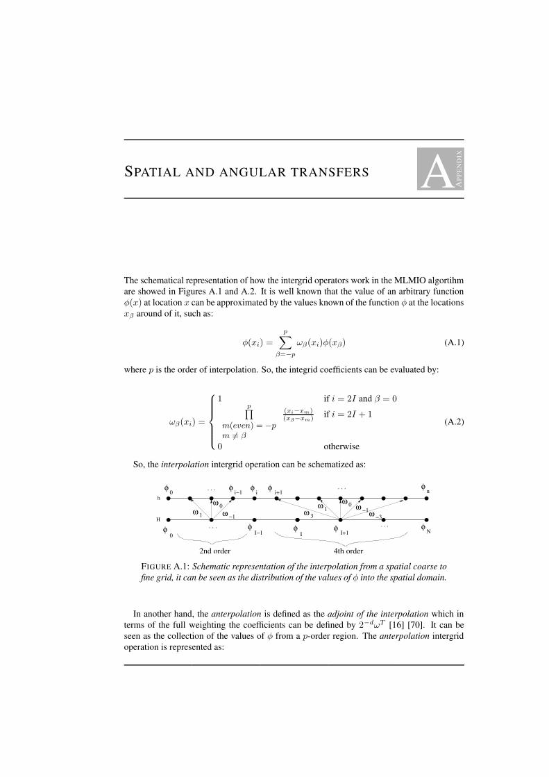
A AP
PE
ND
IX
SPATIAL AND ANGULAR TRANSFERS
The schematical representation of how the intergrid operators work in the MLMIO algortihmare showed in Figures A.1 and A.2. It is well known that the value of an arbitrary functionφ(x) at location x can be approximated by the values known of the function φ at the locationsxβ around of it, such as:
φ(xi) =
p∑
β=−p
ωβ(xi)φ(xβ) (A.1)
where p is the order of interpolation. So, the integrid coefficients can be evaluated by:
ωβ(xi) =
1 if i = 2I and β = 0p∏
m(even) = −p
m 6= β
(xi−xm)(xβ−xm) if i = 2I + 1
0 otherwise
(A.2)
So, the interpolation intergrid operation can be schematized as:
φn
Nφ
2nd order 4th order
φi+1
φi
I+1φ
0φ
φ0
φi−1
Iφ
I−1φ
ω −1
ω 0ω 1 ω −3
ω −1ω 0ω 1ω 3
h
H. . .
. . .. . .
. . .
FIGURE A.1: Schematic representation of the interpolation from a spatial coarse tofine grid, it can be seen as the distribution of the values of φ into the spatial domain.
In another hand, the anterpolation is defined as the adjoint of the interpolation which interms of the full weighting the coefficients can be defined by 2−dωT [16] [70]. It can beseen as the collection of the values of φ from a p-order region. The anterpolation intergridoperation is represented as:
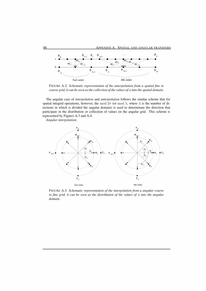
86 APPENDIX A. SPATIAL AND ANGULAR TRANSFERS
h
H
2nd order 4th order
φnφ
i+1φ
iφ0
φi−1
ω −1
ω 0ω 1
NφI+1
φI
φI−1
φ0
φ
ω −3ω −1
ω 0ω 1ω 3
. . .
. . .. . .
FIGURE A.2: Schematic representation of the anterpolation from a spatial fine tocoarse grid, it can be seen as the collection of the values of φ into the spatial domain.
The angular case of interpolation and anterpolation follows the similar scheme that forspatial integrid operations, however, the mod 2π (or mod λ, where λ is the number of di-rections in which is divided the angular domain) is used to determinate the direction thatparticipate in the distribution or collection of values on the angular grid. This scheme isrepresented by Figures A.3 and A.4.
Angular interpolation:
ΦΛΦΛ
W−1
W0
W1
Φ M+1
φλ
Φ M
Φ0φ
m+1 φm+1
φm
φm
φ0
φλ
φ0
Φ M+1
ΦM
Φ0W−1
W1 W0
W3
W−3
2nd order 4th order
. . .
. . .
FIGURE A.3: Schematic representation of the interpolation from a angular coarseto fine grid, it can be seen as the distribution of the values of φ into the angulardomain.
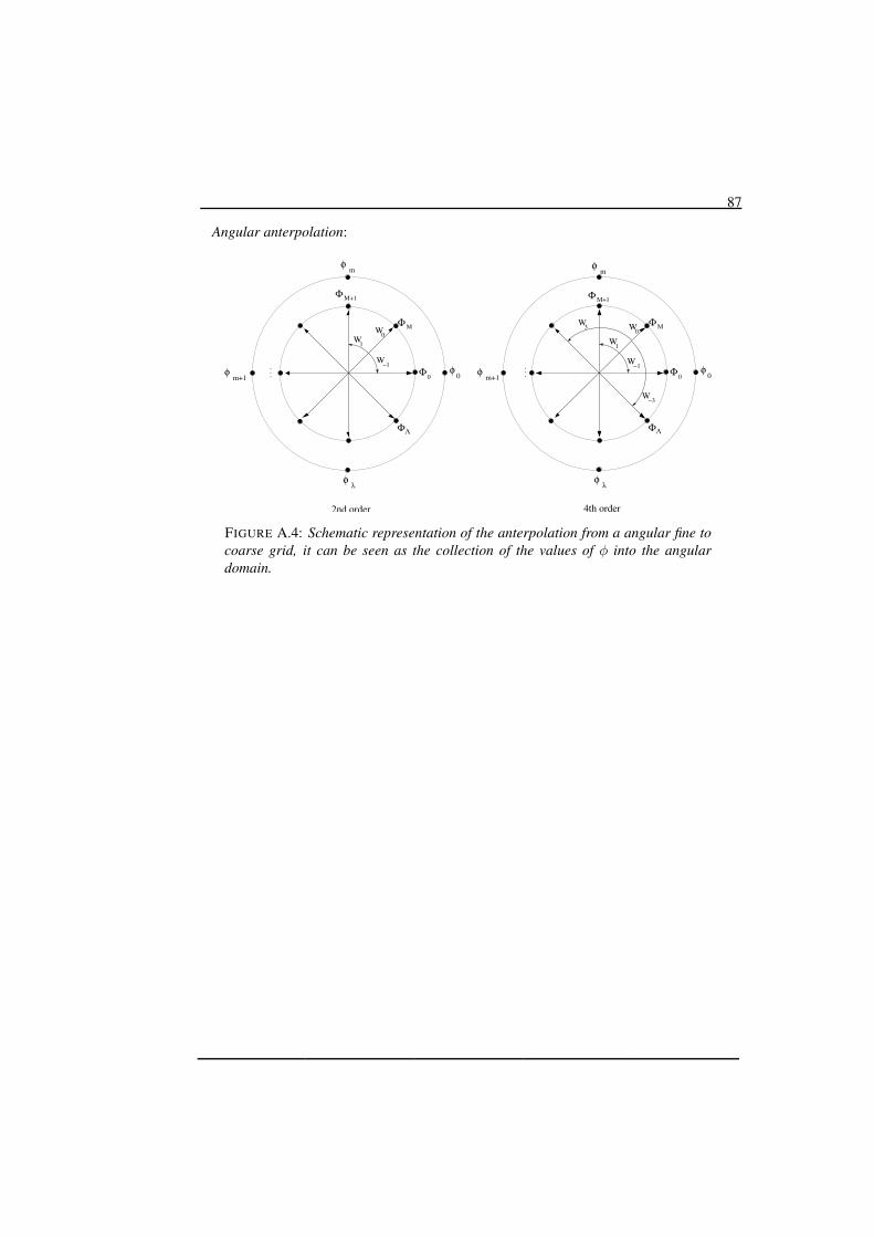
87
Angular anterpolation:
ΦΛΦΛ
W−1
W0W1
Φ0
Φ M+1
φ0φ
m+1
φm
φλ
Φ M
φλ
φm
φm+1
φ0Φ0
Φ M+1
Φ M
W−3
W−1
W0
W1
W3
. . .
2nd order 4th order. .
.
FIGURE A.4: Schematic representation of the anterpolation from a angular fine tocoarse grid, it can be seen as the collection of the values of φ into the angulardomain.

88 APPENDIX A. SPATIAL AND ANGULAR TRANSFERS

B AP
PE
ND
IXRESULTS OF THE MLMIOALGORITHM
In this appendix are shown the way in that the discrete coefficients of the function G(x, y)are determinated for each one of the problems showed in the chpater four. Furthermore,anlaytical solution for the first and second model problems of is provided. Additionally,tables with the norm of the error, computational time and fast evaluation error for the modelproblems showed in the chaper four are presented here.
B.1 First model problem
B.1-A) Exact analytical solution of (4.1)The exact analytical solution of (4.1) is defined as:
v(x) = vp(x) + vn(x) (B.1)
with,
vp(x) = e−ikx[
(1 − b2)c2 − c3 + c4b]
eikb cos(x − b)
−[
(1 − x2)c2 − c3 + c4x]
eikx
+[
(b2 − 1)c1 + c5 − c6b]
eikb sin(x − b) (B.2)
vn(x) = eikx[
(x2 − 1)c2 + c3 + c4x]
e−ikx
−[
(a2 − 1)c2 + c3 + c4a]
e−ika cos(x − a)
−[
(a2 − 1)c1 + c5 + c6a]
e−ika sin(x − a) (B.3)
where the constants are detfined as:
c1 =1
1 − k2c2 = ikc1
c3 = 2i(−k3 − 3k)c1 c4 = 2(−1 − k2)c21
c5 = 2(−1 − 3k2)c31 c6 = 4ikc2
1 (B.4)
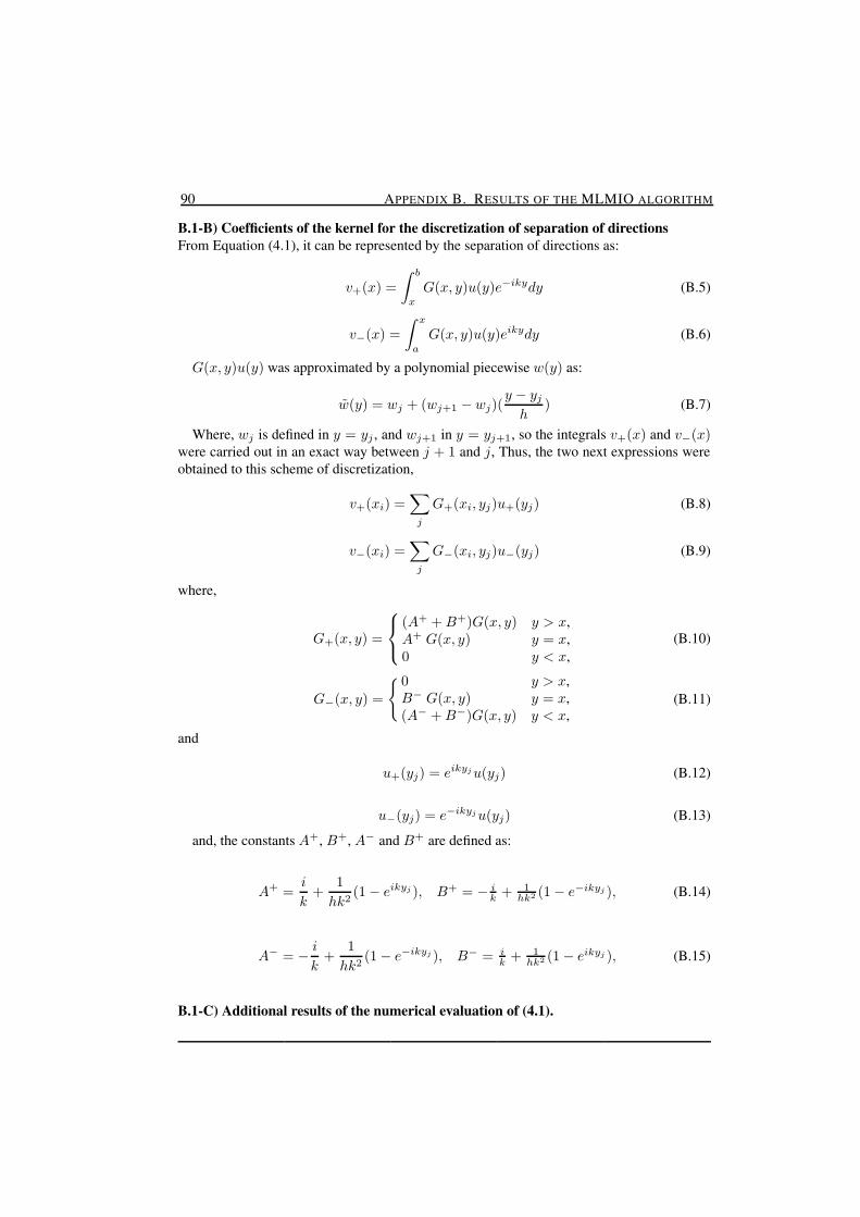
90 APPENDIX B. RESULTS OF THE MLMIO ALGORITHM
B.1-B) Coefficients of the kernel for the discretization of separation of directionsFrom Equation (4.1), it can be represented by the separation of directions as:
v+(x) =
∫ b
x
G(x, y)u(y)e−ikydy (B.5)
v−(x) =
∫ x
a
G(x, y)u(y)eikydy (B.6)
G(x, y)u(y) was approximated by a polynomial piecewise w(y) as:
w(y) = wj + (wj+1 − wj)(y − yj
h) (B.7)
Where, wj is defined in y = yj , and wj+1 in y = yj+1, so the integrals v+(x) and v−(x)were carried out in an exact way between j + 1 and j, Thus, the two next expressions wereobtained to this scheme of discretization,
v+(xi) =∑
j
G+(xi, yj)u+(yj) (B.8)
v−(xi) =∑
j
G−(xi, yj)u−(yj) (B.9)
where,
G+(x, y) =
(A+ + B+)G(x, y) y > x,A+ G(x, y) y = x,0 y < x,
(B.10)
G−(x, y) =
0 y > x,B− G(x, y) y = x,(A− + B−)G(x, y) y < x,
(B.11)
and
u+(yj) = eikyj u(yj) (B.12)
u−(yj) = e−ikyj u(yj) (B.13)
and, the constants A+, B+, A− and B+ are defined as:
A+ =i
k+
1
hk2(1 − eikyj ), B+ = − i
k + 1hk2 (1 − e−ikyj ), (B.14)
A− = − i
k+
1
hk2(1 − e−ikyj ), B− = i
k + 1hk2 (1 − eikyj ), (B.15)
B.1-C) Additional results of the numerical evaluation of (4.1).

§B.1. FIRST MODEL PROBLEM 91
k = 8π1st Scheme of Discretization 2nd Scheme of Discretization
fl Mesh ||ε||2 cpu time [sec.] ||ε||2 cpu time [sec.]5 64 7.19e-05 <1.00e-02 2.01e-05 <1.00e-026 128 1.79e-05 <1.00e-02 5.00e-06 <1.00e-027 256 4.46e-06 <1.00e-02 1.25e-06 <1.00e-028 512 1.11e-06 <1.00e-02 3.11e-07 1.00e-029 1024 2.79e-07 1.00e-02 7.78e-08 1.00e-0210 2048 6.97e-08 4.00e-02 1.95e-08 3.00e-0211 4096 1.74e-08 1.30e-01 4.86e-09 1.40e-0112 8192 4.36e-09 5.40e-01 1.22e-09 5.50e-0113 16384 1.09e-09 2.25e+00 3.04e-10 3.10e+0014 32768 2.72e-10 1.10e+01 7.48e-11 1.60e+0115 65536 6.81e-11 4.75e+01 2.02e-11 6.37e+01
TABLE B.1: Average norm of the error and cpu time for both discretizations (1st discretiza-tion: Single Matrix Multiplication. 2nd discretization: Separation of Directions)(k = 8π).
k = 32π1st Scheme of Discretization 2nd Scheme of Discretization
No. Mesh ||ε|| cpu time [sec.] ||ε|| cpu time [sec.]7 256 4.49e-06 <1.00e-02 3.12e-07 <1.00e-028 512 1.11e-06 <1.00e-02 7.75e-08 <1.00e-029 1024 2.77e-07 1.00e-02 1.93e-08 1.00e-0210 2048 6.93e-08 4.00e-02 4.83e-09 3.00e-0211 4096 1.73e-08 1.40e-01 1.21e-09 1.40e-0112 8192 4.33e-09 5.30e-01 3.02e-10 5.50e-0113 16384 1.08e-09 2.15e+00 7.54e-11 3.19e+0014 32768 2.71e-10 1.11e+01 1.88e-11 1.61e+0115 65536 6.77e-11 4.83e+01 4.77e-12 6.44e+0116 131072 1.69e-11 1.98e+02 9.13e-13 2.56e+02
TABLE B.2: Average norm of the error and cpu time for both discretizations (1st discretiza-tion: Single Matrix Multiplication. 2nd discretization: Separation of Directions)(k = 32π).
||ε||2, k = 8πfl Mesh cl=fl cl=fl-1 cl=fl-2 cl=fl-3 cl=fl-4 cl=fl-55 64 2.01e-05 2.01e-05 2.01e-05 2.01e-05* 2.01e-056 128 5.00e-06 5.00e-06 5.00e-06 5.00e-06 5.00e-06 5.00e-067 256 1.25e-06 1.25e-06 1.25e-06 1.25e-06 1.25e-06* 1.25e-068 512 3.11e-07 3.11e-07 3.11e-07 3.11e-07 3.11e-07 3.11e-079 1024 7.78e-08 7.78e-08 7.78e-08 7.78e-08 7.78e-08 7.78e-08*10 2048 1.95e-08 1.95e-08 1.95e-08 1.95e-08 1.95e-08 1.95e-0811 4096 4.86e-09 4.86e-09 4.86e-09 4.86e-09 4.86e-09 4.86e-0912 8192 1.22e-09 1.22e-09 1.22e-09 1.22e-09 1.22e-09 1.22e-0913 16384 3.04e-10 3.04e-10 3.04e-10 3.04e-10 3.04e-10 3.04e-1014 32768 7.48e-11 7.48e-11 7.48e-11 7.48e-11 7.48e-11 7.48e-1115 65536 2.02e-11 2.02e-11 2.02e-11 2.02e-11 2.02e-11 2.02e-11
TABLE B.3: Average norm of the error in the numerical evaluation of (4.1) using the MLMIOalgorithm with p = 8 order transfers. (k = 8π)
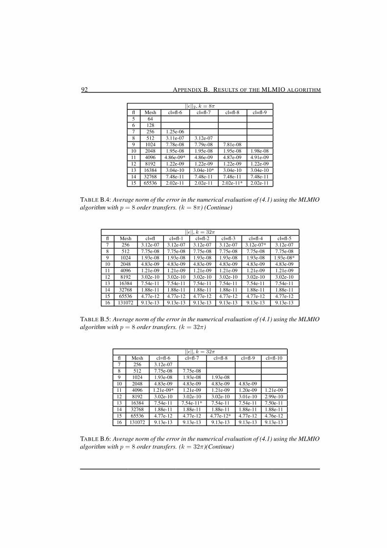
92 APPENDIX B. RESULTS OF THE MLMIO ALGORITHM
||ε||2, k = 8πfl Mesh cl=fl-6 cl=fl-7 cl=fl-8 cl=fl-95 646 1287 256 1.25e-068 512 3.11e-07 3.12e-079 1024 7.78e-08 7.79e-08 7.81e-0810 2048 1.95e-08 1.95e-08 1.95e-08 1.98e-0811 4096 4.86e-09* 4.86e-09 4.87e-09 4.91e-0912 8192 1.22e-09 1.22e-09 1.22e-09 1.22e-0913 16384 3.04e-10 3.04e-10* 3.04e-10 3.04e-1014 32768 7.48e-11 7.48e-11 7.48e-11 7.48e-1115 65536 2.02e-11 2.02e-11 2.02e-11* 2.02e-11
TABLE B.4: Average norm of the error in the numerical evaluation of (4.1) using the MLMIOalgorithm with p = 8 order transfers. (k = 8π) (Continue)
||ε||, k = 32πfl Mesh cl=fl cl=fl-1 cl=fl-2 cl=fl-3 cl=fl-4 cl=fl-57 256 3.12e-07 3.12e-07 3.12e-07 3.12e-07 3.12e-07* 3.12e-078 512 7.75e-08 7.75e-08 7.75e-08 7.75e-08 7.75e-08 7.75e-089 1024 1.93e-08 1.93e-08 1.93e-08 1.93e-08 1.93e-08 1.93e-08*10 2048 4.83e-09 4.83e-09 4.83e-09 4.83e-09 4.83e-09 4.83e-0911 4096 1.21e-09 1.21e-09 1.21e-09 1.21e-09 1.21e-09 1.21e-0912 8192 3.02e-10 3.02e-10 3.02e-10 3.02e-10 3.02e-10 3.02e-1013 16384 7.54e-11 7.54e-11 7.54e-11 7.54e-11 7.54e-11 7.54e-1114 32768 1.88e-11 1.88e-11 1.88e-11 1.88e-11 1.88e-11 1.88e-1115 65536 4.77e-12 4.77e-12 4.77e-12 4.77e-12 4.77e-12 4.77e-1216 131072 9.13e-13 9.13e-13 9.13e-13 9.13e-13 9.13e-13 9.13e-13
TABLE B.5: Average norm of the error in the numerical evaluation of (4.1) using the MLMIOalgorithm with p = 8 order transfers. (k = 32π)
||ε||, k = 32πfl Mesh cl=fl-6 cl=fl-7 cl=fl-8 cl=fl-9 cl=fl-107 256 3.12e-078 512 7.75e-08 7.75e-089 1024 1.93e-08 1.93e-08 1.93e-0810 2048 4.83e-09 4.83e-09 4.83e-09 4.83e-0911 4096 1.21e-09* 1.21e-09 1.21e-09 1.20e-09 1.21e-0912 8192 3.02e-10 3.02e-10 3.02e-10 3.01e-10 2.99e-1013 16384 7.54e-11 7.54e-11* 7.54e-11 7.54e-11 7.50e-1114 32768 1.88e-11 1.88e-11 1.88e-11 1.88e-11 1.88e-1115 65536 4.77e-12 4.77e-12 4.77e-12* 4.77e-12 4.76e-1216 131072 9.13e-13 9.13e-13 9.13e-13 9.13e-13 9.13e-13
TABLE B.6: Average norm of the error in the numerical evaluation of (4.1) using the MLMIOalgorithm with p = 8 order transfers. (k = 32π)(Continue)

§B.2. SECOND MODEL PROBLEM 93
B.2 Second model problemB.2-A) Exact analytical solution of (4.13).The analytical solution for (4.13) is represented by:
v(x) =
vp(x), if x = avn(x), if x = bvp(x) + vn(x), otherwise.
(B.16)
with,
vp(x) = 1k3
π[−1 −1
2k
2(1 − x2)] + 2kx(c1 − 1) + ke
ik(b−x)[b + x + 2a ln(b − x)]
−2kxE1(ik(x − b)) + i[3(1 − eik(b−x)) + c1(k
2x
2 + c2) + πkx
+c4 ln(b − x)eik(b−x) + (k2x
2 + c2)E1(ik(x − b))] (B.17)
vn(x) = 1k3
π[−1 −1
2k
2(1 − x2)] + 2kx(c1 − 1) + ke
ik(x−a)[a − x + 2a ln(x − a)]
+2kxE1(ik(a − x)) + i[3(1 − eik(x−a)) + c1(k
2x
2 + c2) − πkx
+c3 ln(x − a)eik(x−a) + (k2x
2 + c2)E1(ik(a − x))] (B.18)
where the constants are defined as:
c1 = γ ln(k) c2 = −k2 − 2
c3 = k2a2 + c2 c4 = k2b2 + c2 (B.19)
Here γ = 0.577215664901532... which is the Euler constant and E1(z) represents theexponential integral defined as[1]:
E1(z) =
∫ ∞
1
e−zt
tdt =
∫ ∞
z
e−t
tdt (|arg z| < π) (B.20)
Numerical evaluation of the exponential integral is suggested to be performed [75] usingseries expansions for (|z| ≤ 1):
E1(z) = −γ − ln(z) −∞∑
n=1
(−1)n zn
nn!(|arg z| < π)
and continued fractions for the arguments (|z| > 1) :
En(z) = e−z
(
1
z+
n
1+
1
z+
n + 1
1+
2
z+...
)
(|arg z| < π)
with n = 1.
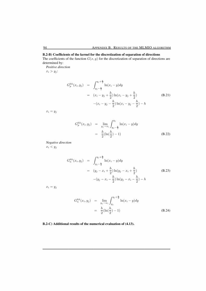
94 APPENDIX B. RESULTS OF THE MLMIO ALGORITHM
B.2-B) Coefficients of the kernel for the discretization of separation of directionsThe coefficients of the function G(x, y) for the discretization of separation of directions aredetermined by:
Positive directionxi > yj :
Ghhp (xi, yj) =
∫ yj+ h2
yj−h2
ln(xi − y)dy
= (xi − yj +h
2) ln(xi − yj +
h
2) (B.21)
−(xi − yj −h
2) ln(xi − yj −
h
2) − h
xi = yj
Ghhp (xi, yj) = lim
yj→xi
∫ yj
yj−h2
ln(xi − y)dy
=h
2(ln(
h
2) − 1) (B.22)
Negative directionxi < yj
Ghhn (xi, yj) =
∫ yj+ h2
yj−h2
ln(xi − y)dy
= (yj − xi +h
2) ln(yj − xi +
h
2) (B.23)
−(yj − xi −h
2) ln(yj − xi −
h
2) − h
xi = yj
Ghhn (xi, yj) = lim
yj→xi
∫ yj+ h2
yj
ln(xi − y)dy
=h
2(ln(
h
2) − 1) (B.24)
B.2-C) Additional results of the numerical evaluation of (4.13).
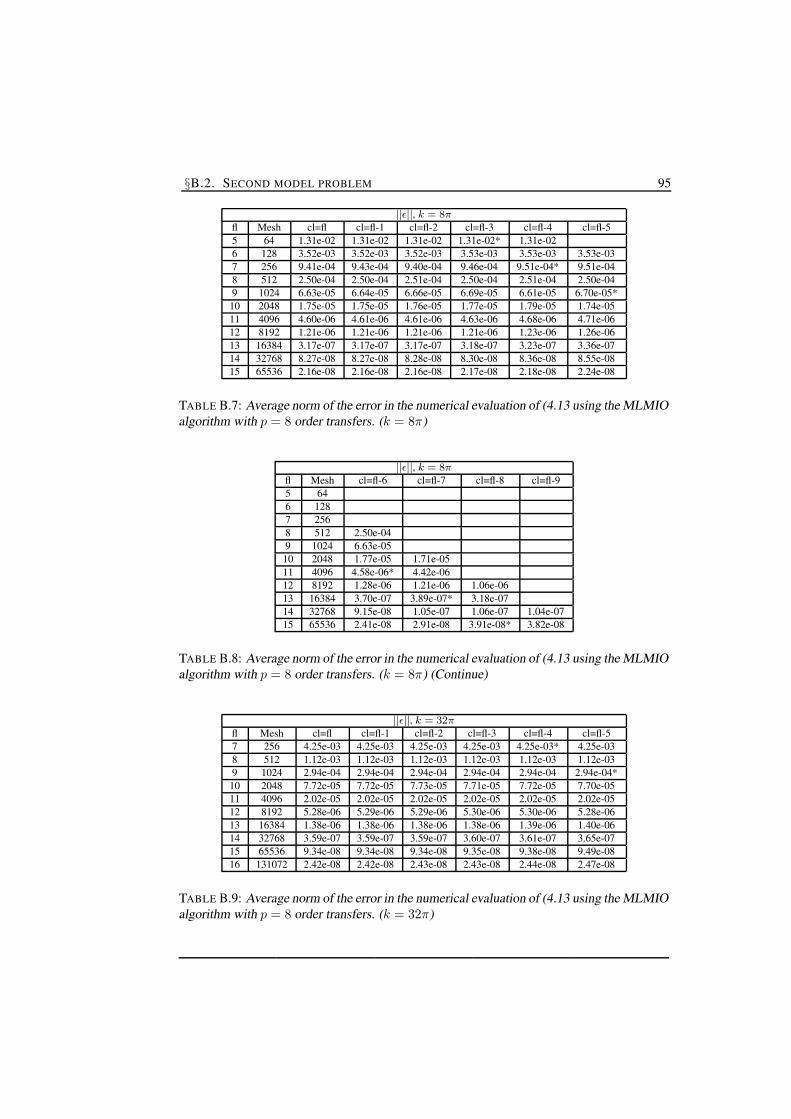
§B.2. SECOND MODEL PROBLEM 95
||ε||, k = 8πfl Mesh cl=fl cl=fl-1 cl=fl-2 cl=fl-3 cl=fl-4 cl=fl-55 64 1.31e-02 1.31e-02 1.31e-02 1.31e-02* 1.31e-026 128 3.52e-03 3.52e-03 3.52e-03 3.53e-03 3.53e-03 3.53e-037 256 9.41e-04 9.43e-04 9.40e-04 9.46e-04 9.51e-04* 9.51e-048 512 2.50e-04 2.50e-04 2.51e-04 2.50e-04 2.51e-04 2.50e-049 1024 6.63e-05 6.64e-05 6.66e-05 6.69e-05 6.61e-05 6.70e-05*10 2048 1.75e-05 1.75e-05 1.76e-05 1.77e-05 1.79e-05 1.74e-0511 4096 4.60e-06 4.61e-06 4.61e-06 4.63e-06 4.68e-06 4.71e-0612 8192 1.21e-06 1.21e-06 1.21e-06 1.21e-06 1.23e-06 1.26e-0613 16384 3.17e-07 3.17e-07 3.17e-07 3.18e-07 3.23e-07 3.36e-0714 32768 8.27e-08 8.27e-08 8.28e-08 8.30e-08 8.36e-08 8.55e-0815 65536 2.16e-08 2.16e-08 2.16e-08 2.17e-08 2.18e-08 2.24e-08
TABLE B.7: Average norm of the error in the numerical evaluation of (4.13 using the MLMIOalgorithm with p = 8 order transfers. (k = 8π)
||ε||, k = 8πfl Mesh cl=fl-6 cl=fl-7 cl=fl-8 cl=fl-95 646 1287 2568 512 2.50e-049 1024 6.63e-0510 2048 1.77e-05 1.71e-0511 4096 4.58e-06* 4.42e-0612 8192 1.28e-06 1.21e-06 1.06e-0613 16384 3.70e-07 3.89e-07* 3.18e-0714 32768 9.15e-08 1.05e-07 1.06e-07 1.04e-0715 65536 2.41e-08 2.91e-08 3.91e-08* 3.82e-08
TABLE B.8: Average norm of the error in the numerical evaluation of (4.13 using the MLMIOalgorithm with p = 8 order transfers. (k = 8π) (Continue)
||ε||, k = 32πfl Mesh cl=fl cl=fl-1 cl=fl-2 cl=fl-3 cl=fl-4 cl=fl-57 256 4.25e-03 4.25e-03 4.25e-03 4.25e-03 4.25e-03* 4.25e-038 512 1.12e-03 1.12e-03 1.12e-03 1.12e-03 1.12e-03 1.12e-039 1024 2.94e-04 2.94e-04 2.94e-04 2.94e-04 2.94e-04 2.94e-04*10 2048 7.72e-05 7.72e-05 7.73e-05 7.71e-05 7.72e-05 7.70e-0511 4096 2.02e-05 2.02e-05 2.02e-05 2.02e-05 2.02e-05 2.02e-0512 8192 5.28e-06 5.29e-06 5.29e-06 5.30e-06 5.30e-06 5.28e-0613 16384 1.38e-06 1.38e-06 1.38e-06 1.38e-06 1.39e-06 1.40e-0614 32768 3.59e-07 3.59e-07 3.59e-07 3.60e-07 3.61e-07 3.65e-0715 65536 9.34e-08 9.34e-08 9.34e-08 9.35e-08 9.38e-08 9.49e-0816 131072 2.42e-08 2.42e-08 2.43e-08 2.43e-08 2.44e-08 2.47e-08
TABLE B.9: Average norm of the error in the numerical evaluation of (4.13 using the MLMIOalgorithm with p = 8 order transfers. (k = 32π)

96 APPENDIX B. RESULTS OF THE MLMIO ALGORITHM
||ε||, k = 32πfl Mesh cl=fl-6 cl=fl-7 cl=fl-8 cl=fl-9 cl=fl-107 2568 512 1.12e-039 1024 2.94e-0410 2048 7.70e-05 7.70e-0511 4096 2.02e-05* 2.02e-0512 8192 5.24e-06 5.28e-06 5.28e-0613 16384 1.38e-06 1.34e-06* 1.38e-0614 32768 3.64e-07 3.63e-07 3.53e-07 3.41e-0715 65536 9.76e-08 9.69e-08 9.77e-08* 9.61e-0816 131072 2.59e-08 2.85e-08 2.79e-08 2.90e-08 3.07e-08
TABLE B.10: Average norm of the error in the numerical evaluation of (4.13 using theMLMIO algorithm with p = 8 order transfers. (k = 32π) (Continue)
||FEε||, k = 8πfl Mesh Disc. Err. cl=fl-1 cl=fl-2 cl=fl-3 cl=fl-4 cl=fl-55 64 1.31e-02 1.38e-05 2.85e-05 3.14e-05* 3.14e-056 128 3.52e-03 8.29e-06 4.70e-06 1.90e-05 2.18e-05 2.18e-057 256 9.41e-04 2.03e-06 3.66e-06 5.04e-06 1.07e-05* 1.13e-058 512 2.50e-04 2.34e-07 5.85e-07 4.71e-07 1.38e-06 2.03e-069 1024 6.63e-05 1.18e-07 3.34e-07 6.22e-07 3.60e-07 1.34e-06*10 2048 1.75e-05 3.77e-08 1.10e-07 2.40e-07 3.89e-07 1.46e-0711 4096 4.60e-06 6.31e-09 1.87e-08 4.25e-08 8.32e-08 1.16e-0712 8192 1.21e-06 2.24e-09 6.66e-09 1.54e-08 3.21e-08 5.99e-0813 16384 3.17e-07 1.12e-09 3.33e-09 7.73e-09 1.64e-08 3.31e-0814 32768 8.27e-08 2.32e-10 6.90e-10 1.60e-09 3.42e-09 7.01e-0915 65536 2.16e-08 8.76e-11 2.61e-10 6.07e-10 1.30e-09 2.67e-09
TABLE B.11: Norm of the fast evaluation error of (4.13) using the MLMIO algorithm withp = 8 order transfers. (k = 8π)
||FEε||, k = 8πfl Mesh cl=fl-6 cl=fl-7 cl=fl-8 cl=fl-95 646 1287 2568 512 1.86e-069 1024 1.91e-0610 2048 8.05e-07 7.75e-0711 4096 4.98e-08* 2.10e-0712 8192 7.76e-08 4.81e-08 1.52e-0713 16384 6.06e-08 7.48e-08* 4.91e-0814 32768 1.38e-08 2.43e-08 2.27e-08 3.07e-0815 65536 5.39e-09 1.05e-08 1.82e-08* 1.66e-08
TABLE B.12: Norm of the fast evaluation error of (4.13) using the MLMIO algorithm withp = 8 order transfers. (k = 8π) (Continue)
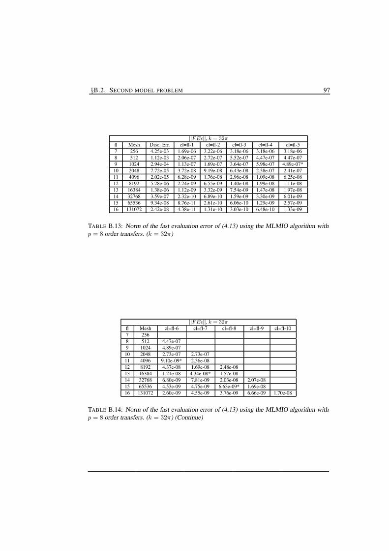
§B.2. SECOND MODEL PROBLEM 97
||FEε||, k = 32πfl Mesh Disc. Err. cl=fl-1 cl=fl-2 cl=fl-3 cl=fl-4 cl=fl-57 256 4.25e-03 1.69e-06 3.22e-06 3.18e-06 3.18e-06 3.18e-068 512 1.12e-03 2.06e-07 2.72e-07 5.52e-07 4.47e-07 4.47e-079 1024 2.94e-04 1.13e-07 1.69e-07 3.64e-07 5.98e-07 4.89e-07*10 2048 7.72e-05 3.72e-08 9.19e-08 6.43e-08 2.38e-07 2.41e-0711 4096 2.02e-05 6.28e-09 1.76e-08 2.96e-08 1.09e-08 6.25e-0812 8192 5.28e-06 2.24e-09 6.55e-09 1.40e-08 1.99e-08 1.11e-0813 16384 1.38e-06 1.12e-09 3.32e-09 7.54e-09 1.47e-08 1.97e-0814 32768 3.59e-07 2.32e-10 6.89e-10 1.59e-09 3.30e-09 6.01e-0915 65536 9.34e-08 8.76e-11 2.61e-10 6.06e-10 1.29e-09 2.57e-0916 131072 2.42e-08 4.38e-11 1.31e-10 3.03e-10 6.48e-10 1.33e-09
TABLE B.13: Norm of the fast evaluation error of (4.13) using the MLMIO algorithm withp = 8 order transfers. (k = 32π)
||FEε||, k = 32πfl Mesh cl=fl-6 cl=fl-7 cl=fl-8 cl=fl-9 cl=fl-107 2568 512 4.47e-079 1024 4.89e-0710 2048 2.73e-07 2.73e-0711 4096 9.10e-09* 2.36e-0812 8192 4.37e-08 1.69e-08 2.48e-0813 16384 1.21e-08 4.34e-08* 1.57e-0814 32768 6.80e-09 7.81e-09 2.03e-08 2.07e-0815 65536 4.53e-09 4.75e-09 6.63e-09* 1.69e-0816 131072 2.60e-09 4.55e-09 3.76e-09 6.66e-09 1.70e-08
TABLE B.14: Norm of the fast evaluation error of (4.13) using the MLMIO algorithm withp = 8 order transfers. (k = 32π) (Continue)
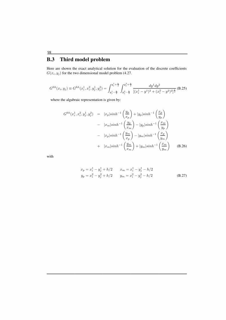
98
B.3 Third model problemHere are shown the exact analytical solution for the evaluation of the discrete coefficientsG(xi, yj) for the two dimensional model problem (4.27.
Ghh(xi, yj) ≡ Ghh(x1i , x
2i , y
1j , y2
j ) =
∫ y1
j + h2
y1
j−h
2
∫ y2
j + h2
y2
j−h
2
dy1dy2
[(x1i − y1)2 + (x2
i − y2)2]1
2
(B.25)
where the algabraic representation is given by:
Ghh(x1i , x
2i , y
1j , y2
j ) = |xp|sinh−1
(
yp
xp
)
+ |yp|sinh−1
(
xp
yp
)
− |xm|sinh−1
(
yp
xm
)
− |yp|sinh−1
(
xm
yp
)
− |xp|sinh−1
(
ym
xp
)
− |ym|sinh−1
(
xp
ym
)
+ |xm|sinh−1
(
ym
xm
)
+ |ym|sinh−1
(
xm
ym
)
(B.26)
with
xp = x1i − y1
j + h/2 xm = x1i − y1
j − h/2
yp = x2i − y2
j + h/2 ym = x2i − y2
j − h/2 (B.27)


![SCATTERING ANALYSIS OF PERIODIC ARRAYS USING COMBINED … · Fourier transform method (CG-FFT) [13], fast multipole algorithm (FMM) or multilevel fast multipole algorithm (MLFMA)](https://static.fdocuments.in/doc/165x107/60a8f556e81d373cf3227d18/scattering-analysis-of-periodic-arrays-using-combined-fourier-transform-method-cg-fft.jpg)


![Twisted Acoustics: Metasurface‐Enabled …(WDM), time-division multiplexing (TDM), and multilevel amplitude/phase modulation,[4–7] data rate of acoustic com-munication is approaching](https://static.fdocuments.in/doc/165x107/5e9bf93695e5e7674e2807ea/twisted-acoustics-metasurfaceaenabled-wdm-time-division-multiplexing-tdm.jpg)

![Harmony Search Optimization Algorithm Based Multilevel ...Harmony Search Optimization Algorithm Based Multilevel Thresholding for MRI Brain Images M.Chithradevi [1], C.Alagurani [2]](https://static.fdocuments.in/doc/165x107/60a027a1dca97a27c9217deb/harmony-search-optimization-algorithm-based-multilevel-harmony-search-optimization.jpg)
![A multilevel bilinear programming algorithm for the vertex ...users.clas.ufl.edu/hager/papers/GP/ml.pdfA multilevel bilinear programming algorithm for the VSP heuristics [29], spectral](https://static.fdocuments.in/doc/165x107/600e1687a1909d67ad528120/a-multilevel-bilinear-programming-algorithm-for-the-vertex-usersclasufleduhagerpapersgpmlpdf.jpg)


![A Multilevel Tabu Search for the Maximum Satisfiability ... · Tabu Search algorithm (TS) was proposed by Glover [17]. The main feature of the algorithm is the ability to avoid returning](https://static.fdocuments.in/doc/165x107/5eafd2ae7437eb58242c2cf9/a-multilevel-tabu-search-for-the-maximum-satisfiability-tabu-search-algorithm.jpg)