C. Chadoulos, P. Kaplanoglou, S. Papadopoulos, Prof. Ioannis Pitas

Aristotle University of Thessaloniki

pitas@csd.auth.gr

www.aiia.csd.auth.grVersion 2.8

Multilayer Perceptron

Backpropagation Summary

Biological Neuron⚫ Basic computational unit of the brain.

⚫ Main parts:

• Dendrites

➔ Act as inputs.

• Soma

➔ Main body of neuron.

• Axon

➔ Acts as output.

⚫ Neurons connect with other neurons via synapses.

2

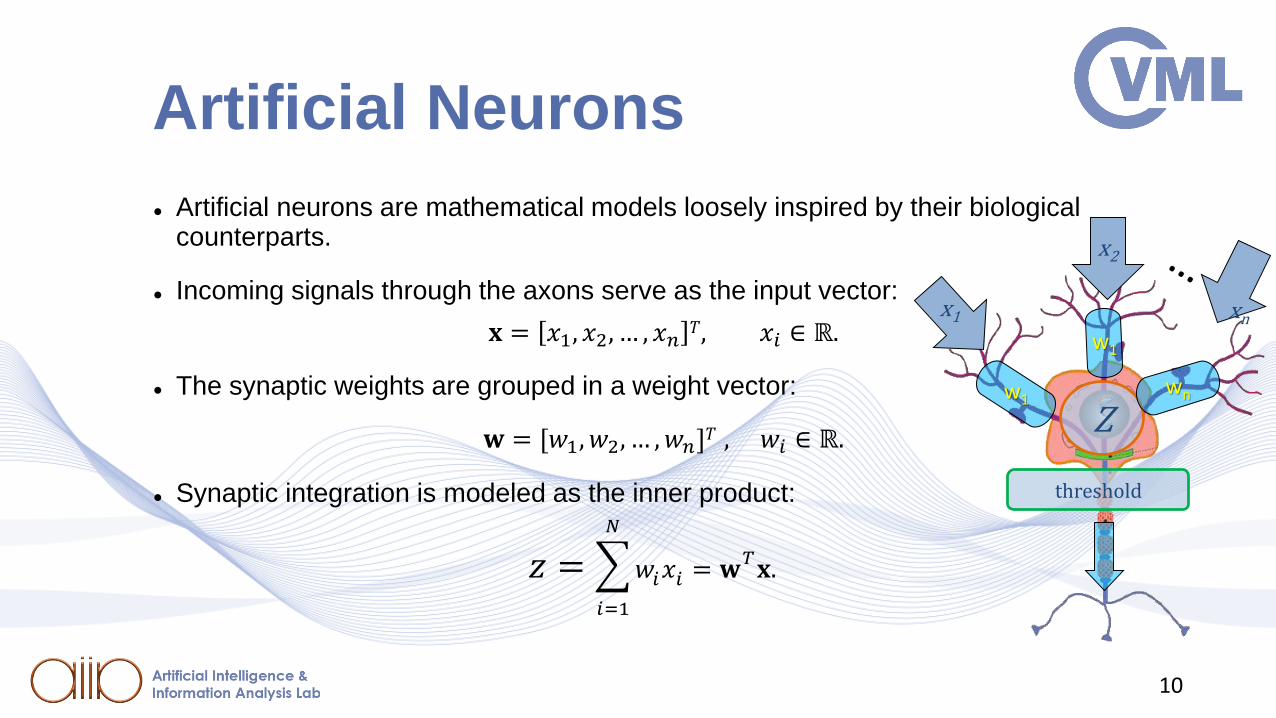
Artificial Neurons

⚫ Artificial neurons are mathematical models loosely inspired by their biological counterparts.

⚫ Incoming signals through the axons serve as the input vector:

𝐱 = 𝑥1, 𝑥2, … , 𝑥𝑛𝑇, 𝑥𝑖 ∈ ℝ.

⚫ The synaptic weights are grouped in a weight vector:

𝐰 = [𝑤1, 𝑤2, … , 𝑤𝑛]𝑇 , 𝑤𝑖 ∈ ℝ.

⚫ Synaptic integration is modeled as the inner product:

𝑧 =

𝑖=1

𝑁

𝑤𝑖𝑥𝑖 = 𝐰𝑇𝐱.

Z

threshold

x1

x2

xn

w1

w1

wn

10

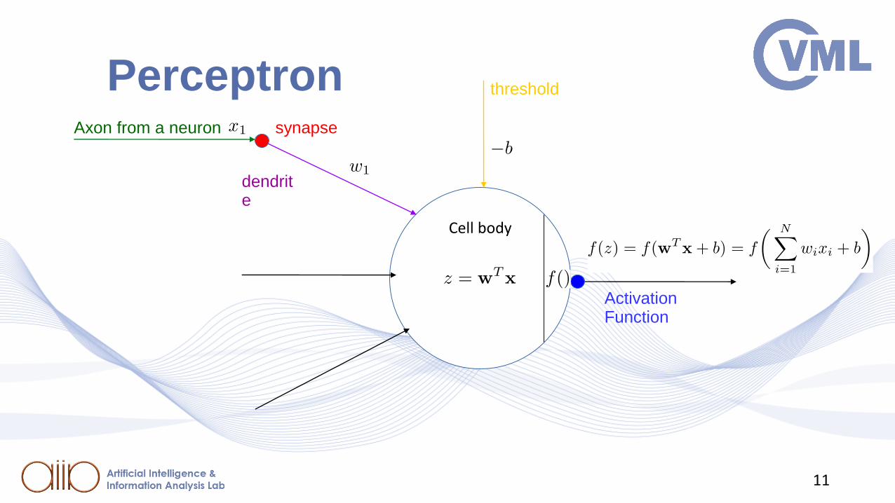
Cell body

synapse

dendrite

Axon from a neuron

Activation Function

Perceptron threshold

11

Perceptron

⚫ Simplest mathematical model of a neuron (Rosenblatt – McCulloch & Pitts)

⚫ Inputs are binary, 𝑥𝑖 ∈ 0,1 .

⚫ Produces single, binary outputs, 𝑦𝑖 ∈ {0,1}, through an activation function 𝑓(∙).

⚫ Output 𝑦𝑖 signifies whether the neuron will fire or not.

⚫ Firing threshold:

𝐰𝑇𝐱 ≥ −𝑏 ⇒ 𝐰𝑇𝐱 + 𝑏 ≥ 0.Cell body

12

MLP Architecture

⚫ Multilayer perceptrons (feed-forward neural networks) typically consist of 𝐿 + 1 layers with 𝑘𝑙 neurons in each layer: 𝑙 = 0,… , 𝐿.

⚫ The first layer (input layer 𝑙 = 0) contains 𝑛 inputs, where 𝑛 is the dimensionality of the input sample vector.

⚫ The 𝐿 − 1 hidden layers 𝑙 = 1,… , 𝐿 − 1 can contain any number of neurons.

26

MLP Architecture

⚫ The output layer 𝑙 = 𝐿 typically contains either one neuron (especially when dealing with regression problems) or 𝑚 neurons, where 𝑚 is the number of classes.

⚫ Thus, neural networks can be described by the following characteristic numbers:

1.Depth: Number of hidden layers 𝐿.

2.Width: Number of neurons per layer 𝑘𝑙 , 𝑙 = 1,… , 𝐿.

3. 𝑘𝐿 = 1, or 𝑘𝐿 = 𝑚.

26

MLP Forward Propagation

.

.

.

.

.

.

𝑧𝑗(𝑙)

𝑧𝑘𝑙(𝑙)

𝑧1(𝑙)

𝑧𝑖(𝑙)

.

.

.

.

.

.

⚫ Following the same procedure for the 𝑙𝑡ℎ hidden layer, we get:

⚫ In compact form:

𝑎1(𝑙)

𝑎𝑖(𝑙)

𝑎𝑗(𝑙)

𝑎𝑘𝑙(𝑙)

𝑓(𝑧1𝑙)

𝑓(𝑧𝑖𝑙)

𝑓(𝑧𝑗𝑙)1

𝑓(𝑧𝑘𝑙𝑙)

.

.

29

MLP Activation Functions⚫ Previous theorem verifies MLPs as universal approximators, under the condition that the

activation functions 𝜙 ∙ for each neuron are continuous.

⚫ Continuous (and differentiable) activation functions:

⚫ 𝜎 𝑥 =1

1+𝑒−𝑥, ℝ𝑛 → 0,1

⚫ 𝑅𝑒𝐿𝑈 𝑥 = ቊ0, 𝑥 < 0𝑥, 𝑥 ≥ 0

, ℝ𝑛 → ℝ+

⚫ 𝑓 𝑥 = tan−1 𝑥 , ℝ𝑛 → Τ−𝜋 2 , Τ𝜋 2

⚫ 𝑓 𝑥 = tanh 𝑥 =𝑒𝑥−𝑒−𝑥

𝑒𝑥+𝑒−𝑥, ℝ𝑛 → −1,+1

25

Softmax Layer

• It is the last layer in a neural network classifier.

• The response of neuron 𝑖 in the softmax layer 𝐿 is calculated with regard to the value of its

activation function 𝑎𝑖 = 𝑓 𝑧𝑖 .

• The responses of softmax neurons sum up to one:

• Better representation for mutually exclusive class labels.

ො𝑦𝑖 = 𝑔 𝑎𝑖 =𝑒𝑎𝑖

σ𝑘=1𝑘𝐿 𝑒𝑎𝑘

: ℝ → 0,1 , 𝑖 = 1, . . , 𝑘𝐿

σ𝑖=1𝑘𝐿 ො𝑦𝑖 = 1.

31

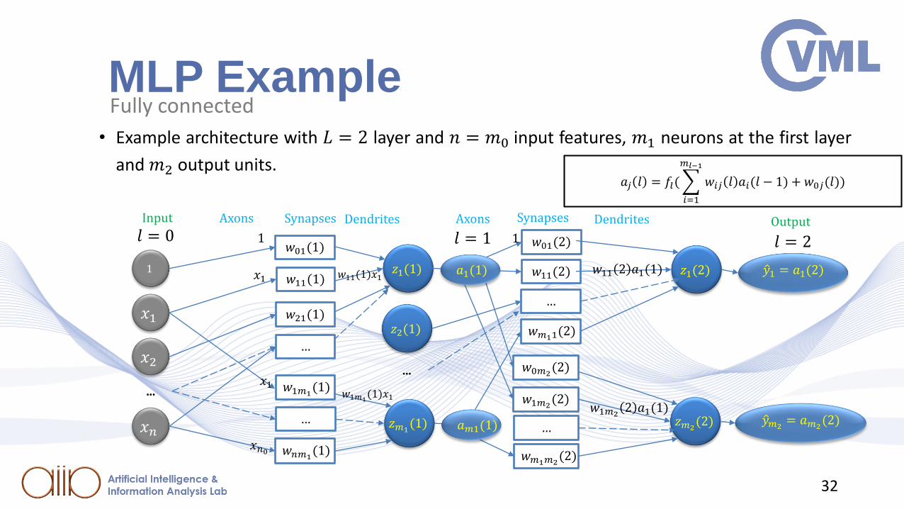
MLP Example• Example architecture with 𝐿 = 2 layer and 𝑛 = 𝑚0 input features, 𝑚1 neurons at the first layer

and 𝑚2 output units.𝑎𝑗 𝑙 = 𝑓𝑙(

𝑖=1

𝑚𝑙−1

𝑤𝑖𝑗 𝑙 𝑎𝑖(𝑙 − 1) + 𝑤0𝑗(𝑙))

𝑥1

𝑥2

𝑥𝑛

1

…

𝑧1(1)

𝑤𝑛𝑚1(1)

𝑤01(1)

𝑤1𝑚1(1)

𝑧𝑚1(1)…

…

𝑥1

𝑤11(1)𝑥1

𝑤1𝑚1(1)𝑥1

DendritesSynapsesAxons Axons

𝑤11(1)

𝑤21(1)

𝑧1(2)

Synapses

𝑤01(2)

𝑤11(2)

1 1

Dendrites

𝑧2(1)

…

𝑧𝑚2(2)…

…

𝑤1𝑚2(2)

𝑥1

𝑤1𝑚22 𝑎1(1)

𝑤11 2 𝑎1(1)

𝑤𝑚1𝑚2(2)

𝑤𝑚11(2)

OutputInput

𝑤0𝑚2(2)

𝑥𝑛0

Fully connected

𝑙 = 0 𝑙 = 1 𝑙 = 2

𝑎1(1)

𝑎𝑚1(1)

ො𝑦1 = 𝑎1(2)

ො𝑦𝑚2= 𝑎𝑚2

(2)

32

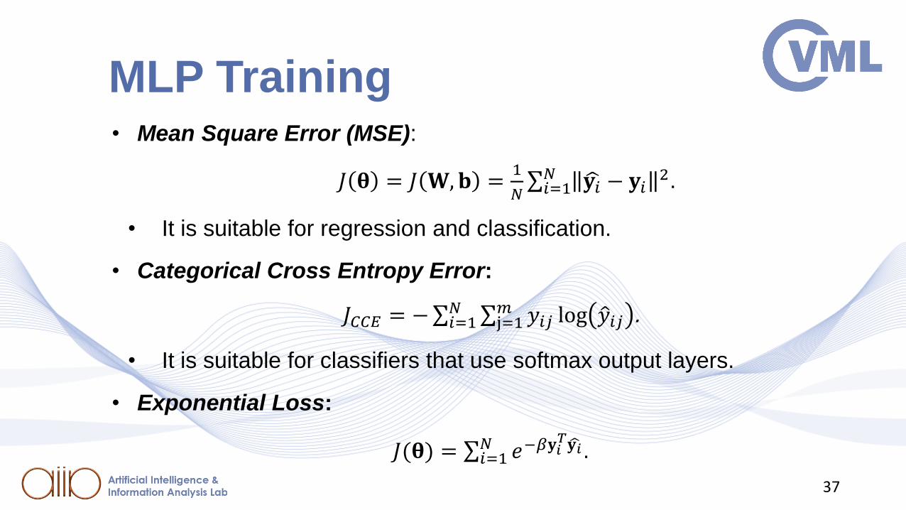
MLP Training • Mean Square Error (MSE):

𝐽 𝛉 = 𝐽 𝐖, 𝐛 =1

𝑁σ𝑖=1𝑁 ෝ𝐲𝑖 − 𝐲𝑖

2.

• It is suitable for regression and classification.

• Categorical Cross Entropy Error:

𝐽𝐶𝐶𝐸 = −σ𝑖=1𝑁 σj=1

𝑚 𝑦𝑖𝑗 log ො𝑦𝑖𝑗 .

• It is suitable for classifiers that use softmax output layers.

• Exponential Loss:

𝐽(𝛉) = σ𝑖=1𝑁 𝑒−𝛽𝐲𝑖

𝑇 ෝ𝐲𝑖.

37

MLP Training

• Differentiation:𝜕𝐽

𝜕𝐖=

𝜕𝐽

𝜕𝐛= 𝟎 can provide the critical points:

• Minima, maxima, saddle points.

• Analytical computations of this kind are usually impossible.

• Need to resort to numerical optimization methods.

38

MLP Training

• Iteratively search the parameter space for the optimal values. In each iteration, apply a small correction to the previous value.

𝛉 𝑡 + 1 = 𝛉 𝑡 + ∆𝛉.

• In the neural network case, jointly optimize 𝐖,𝐛

𝐖 𝑡 + 1 = 𝐖 𝑡 + ∆𝐖,

𝐛 𝑡 + 1 = 𝐛 𝑡 + ∆𝐛.

• What is an appropriate choice for the correction term?

38

MLP Training

Steepest descent on a function surface.

39

MLP Training • Gradient Descent, as applied to Artificial Neural Networks:

• Equations for the 𝑗𝑡ℎ neuron in the 𝑙𝑡ℎ layer:

40

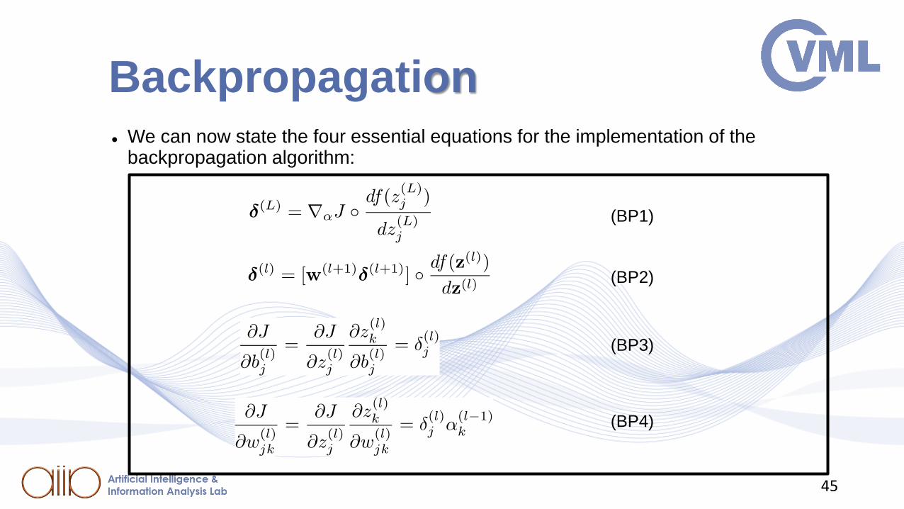
Backpropagation⚫ We can now state the four essential equations for the implementation of the

backpropagation algorithm:

(BP1)

(BP2)

(BP3)

(BP4)

45

Backpropagation Algorithm

46

𝐀𝐥𝐠𝐨𝐫𝐢𝐭𝐡𝐦:Neural Network Training with Gradient Descent and Back propagation

Input: learning rate 𝜇, dataset { 𝐱𝑖 , 𝐲𝑖 }𝑖=1𝑁

𝐑𝐚𝐧𝐝𝐨𝐦 𝐢𝐧𝐢𝐭𝐢𝐚𝐥𝐢𝐳𝐚𝐭𝐢𝐨𝐧 𝐨𝐟 𝐧𝐞𝐭𝐰𝐨𝐫𝐤 𝐩𝐚𝐫𝐚𝐦𝐞𝐭𝐞𝐫𝐬 (𝐖,𝐛)

𝐃𝐞𝐟𝐢𝐧𝐞 𝐜𝐨𝐬𝐭 𝐟𝐮𝐧𝐜𝐭𝐢𝐨𝐧 𝐽 =1

𝑁σ𝑖=1𝑁 𝐲𝑖 − ො𝐲𝑖

2

𝐰𝐡𝐢𝐥𝐞 𝑜𝑝𝑡𝑖𝑚𝑖𝑧𝑎𝑡𝑖𝑜𝑛 𝑐𝑟𝑖𝑡𝑒𝑟𝑖𝑎 𝑛𝑜𝑡 𝑚𝑒𝑡 𝐝𝐨𝐽 = 0𝐅𝐨𝐫𝐰𝐚𝐫𝐝 𝐩𝐚𝐬𝐬 𝐨𝐟 𝐰𝐡𝐨𝐥𝐞 𝐛𝐚𝐭𝐜𝐡 ො𝐲 = 𝐟𝑁𝑁 𝐱;𝐖, 𝐛

𝐽 =1

𝑁

𝑖=1

𝑁

𝐲𝑖 − ො𝐲𝑖2

𝛅 𝐿 = ∇𝑎𝐽 ∘𝑑𝑓 𝑧𝑗

𝐿

𝑑𝑧𝑗𝐿

𝐟𝐨𝐫 𝑙 = 1, … , 𝐿 − 1 𝐝𝐨

𝛅 𝑙 = 𝐰 𝑙+1 𝛅 𝑙+1 ∘𝑑𝑓 𝐳 𝑙

𝑑𝐳 𝑙

𝜕𝐽

𝜕𝑤𝑗𝑘𝑙= 𝛿𝑗

𝑙 𝑎𝑘𝑙−1

𝜕𝐽

𝜕𝑏𝑗𝑙= 𝛿𝑗

𝑙

𝐞𝐧𝐝𝐖 ←𝐖− 𝜇∇𝐰𝐽(𝐖, 𝐛)𝐛 ← 𝐛 − 𝜇∇𝐛𝐽(𝐖, 𝐛)

𝐞𝐧𝐝

Optimization Review

⚫ Batch Gradient Descent problems:

3) Ill conditioning: Takes into account only first – order information (1𝑠𝑡 derivative). No information about curvature of cost function may lead to zig-zagging motions during optimization, resulting in very slow convergence.

4) May depend too strongly on the initialization of the parameters.

5) Learning rate must be chosen very carefully.

48

Optimization Review

⚫ Stochastic Gradient Descent (SGD):

1. Passing the whole dataset through the network just for a small update in the parameters is inefficient.

2.Most cost functions used in Machine Learning and Deep Learning applications can be decomposed into a sum over training samples. Instead of computing the gradient through the whole training set, we decompose the training set {(𝐱𝑖 , 𝐲𝑖), 𝑖 = 1,…𝑁} to 𝐵 mini-batches (possibly same cardinality 𝑆) to estimate 𝛻𝜃𝐽 from 𝛻𝜃𝐽𝑏, 𝑏 = 1,… , 𝐵:

σ𝑠=1𝑆 𝛻𝜃𝐽𝐱𝑠

𝑆≈σ𝑖=1𝑁 𝛻𝜃𝐽𝐱𝑖𝑁

= 𝛻𝜃𝐽 ⇒ 𝛻𝜃𝐽 ≈1

𝑆

𝑠=1

𝑆

𝛻𝜃𝐽𝐱𝑠

49

Optimization Review • Adaptive Learning Rate Algorithms:

• Up to this point, the learning rate was given as an input to the algorithm and was kept stable throughout the whole optimization procedure.

• To overcome the difficulties of using a set rate, adaptive rate algorithms assign a different learning rate for each separate model parameter.

51

Optimization Review • Adaptive Learning Rate Algorithms:

1.AdaGrad algorithm:

i. Gradient accumulation variable 𝐫 = 𝟎

ii.Compute and accumulate gradient 𝐠 ←1

𝑚𝛻𝜽σ𝑖 𝐽 𝑓 𝐱 𝑖 ; 𝛉 𝑖 , 𝐲𝑖 , 𝐫 ← 𝐫 + 𝐠 ∘ 𝐠

iii.Compute update ∆𝛉 ← −𝜇

𝜀+ 𝐫∘ 𝐠 and apply update 𝛉 ← 𝛉 + ∆𝛉

Parameters with largest partial derivative of the loss have a more rapid decrease in their learning rate. ○ denotes element-wise multiplication.

51

Generalization• Good performance on the training set alone is not a satisfying indicator of a good model.

• We are interested in building models that can perform well on data they have not been used the training process. Bad generalization capabilities mainly occur through 2 forms:

1.Overfitting:

• Overfitting can be detected when there is great discrepancy between the performance of the model in the training set, and that in any other set. It can happen due to excessive model complexity.

• An example of overfitting would be trying to model a quadratic equation with a 10-th degree polynomial.

54

Generalization2.Underfitting:

• On the other hand, underfitting occurs when a model cannot accurately capture the underlying structrure of data.

• Underfitting can be detected by a very low performance in the training set.

• Example: trying to model a non-linear equation using linear ones.

55

Revisiting Activation Functions• To overcome the shortcomings of the sigmoid activation function, the Rectified Linear

Unit (ReLU) was introduced.

• Very easy to compute.

• Due to its quasi-linear form leads to faster convergence (does not saturate at high values)

• Units with zero derivative will not activate at all.

59

Training on Large Scale Datasets

• Large number of training samples in the magnitude of hundreds of thousands.

• Problem: Datasets do not fit in memory.

• Solution: Using mini-batch SGD method.

• Many classes, in the magnitude of hundreds up to one thousand.

• Problem: Difficult to converge using MSE error.

• Solution: Using Categorical Cross Entropy (CCE) loss on Softmax output.

60

Towards Deep Learning⚫ Increasing the network depth (layer number) 𝐿 can result in negligible weight updates

in the first layers, because the corresponding deltas become very small or vanish completely

⚫ Problem: Vanishing gradients.

⚫ Solution: Replacing sigmoid with an activation function without an upper bound,

like a rectifier (a.k.a. ramp function, ReLU).

• Full connectivity has high demands for memory and computations

• Very deep fully connected DNNs are difficult to implement.

• New architectures come into play (Convolutional Neural Networks, Deep Autoencoders etc.)

61

Bibliography[ZUR1992] J.M. Zurada, Introduction to artificial neural systems. Vol. 8. St. Paul: West publishing company, 1992.

[JAIN1996] Jain, Anil K., Jianchang Mao, and K. Moidin Mohiuddin. "Artificial neural networks: A tutorial." Computer 29.3 (1996): 31-44.

[YEG2009] Yegnanarayana, Bayya. Artificial neural networks. PHI Learning Pvt. Ltd., 2009.

[DAN2013] Daniel, Graupe. Principles of artificial neural networks. Vol. 7. World Scientific, 2013.

[HOP1988] Hopfield, John J. "Artificial neural networks." IEEE Circuits and Devices Magazine 4.5 (1988): 3-10.

62

Bibliography[HAY2009] S. Haykin, Neural networks and learning machines, Prentice Hall, 2009.[BIS2006] C.M. Bishop, Pattern recognition and machine learning, Springer, 2006.[GOO2016] I. Goodfellow, Y. Bengio, A. Courville, Deep learning, MIT press, 2016[THEO2011] S. Theodoridis, K. Koutroumbas, Pattern Recognition, Elsevier, 2011.[ZUR1992] J.M. Zurada, Introduction to artificial neural systems. Vol. 8. St. Paul: West publishing

company, 1992.[ROS1958] Rosenblatt, Frank. "The perceptron: a probabilistic model for information storage and

organization in the brain." Psychological review 65.6 (1958): 386.[YEG2009] Yegnanarayana, Bayya. Artificial neural networks. PHI Learning Pvt. Ltd., 2009.[DAN2013] Daniel, Graupe. Principles of artificial neural networks. Vol. 7. World Scientific, 2013.[HOP1988] Hopfield, John J. "Artificial neural networks." IEEE Circuits and Devices Magazine 4.5

(1988): 3-10.[SZE2013] C. Szegedy, A. Toshev, D. Erhan. "Deep neural networks for object

detection." Advances in neural information processing systems. 2013.[SAL2016] T. Salimans, D. P. Kingma "Weight normalization: A simple reparameterization to

accelerate training of deep neural networks." Advances in Neural Information ProcessingSystems. 2016.

[MII2019] Miikkulainen, Risto, et al. "Evolving deep neural networks." Artificial Intelligence in theAge of Neural Networks and Brain Computing. Academic Press, 2019. 293-312.

63

Q & A

Thank you very much for your attention!

Contact: Prof. I. Pitas

pitas@csd.auth.gr