Multil-level Weiner-Hopf Monte-Carlo simulation for Lévy ... · Multil-level Weiner-Hopf...

Multil-level Weiner-Hopf Monte-Carlo simulation for Levy processes

Multil-level Weiner-Hopf Monte-Carlo simulation for Levyprocesses

A. Ferreiro-Castilla, A.E. Kyprianou, R. Scheichl, G. Suryanarayana

Department of Mathematical Sciences, University of Bath

What is a (one-dimensional) Levy process?

Formally: A stochastic process {Xt : t ≥ 0} which satisfiesX0 = 0,

X has paths that are right-continuous with left limits (almost surely),

For any 0 ≤ s ≤ t , Xt −Xs is equal in distribution to Xt−s ,

For any 0 ≤ s ≤ t , Xt −Xs is independent of {Xu : u ≤ s}.

Informally: Some familiar Levy processes include

Linear Brownian motion: σBt + µt , t ≥ 0, where σ2 ≥ 0 and µ ∈ R,

Compound Poisson processes:∑Nt

i=1 ξi , where {Nt : t ≥ 0} is a Poissonarrival process and {ξi : i ∈ N} are i.i.d. random variables.

If X(1)t , X

(2)t · · · , are independent Levy processes then, subject to certain

conditions, so is ∑i≥1

Informally: Some familiar Levy processes includeLinear Brownian motion: σBt + µt , t ≥ 0, where σ2 ≥ 0 and µ ∈ R,

If X(1)t , X

Informally: Some familiar Levy processes includeLinear Brownian motion: σBt + µt , t ≥ 0, where σ2 ≥ 0 and µ ∈ R,

If X(1)t , X

Brownian motion

0.0 0.2 0.4 0.6 0.8 1.0

Compound Poisson process

0.0 0.2 0.4 0.6 0.8 1.0

Brownian motion + compound Poisson process

0.0 0.2 0.4 0.6 0.8 1.0!0.1

Unbounded variation paths

0.0 0.2 0.4 0.6 0.8 1.0

Bounded variation paths

0.0 0.2 0.4 0.6 0.8 1.0

Motivation

Levy process. A (one dimensional) process with stationary andindependent increments which has paths which are right continuous withleft limits and therefore includes Brownian motion with drift, compoundPoisson processes, stable processes amongst many others).

A popular (and often criticised) model in mathematical finance for theevolution of a risky asset is

St := eXt , t ≥ 0

where {Xt : t ≥ 0} is a Levy process. Also used in insurance risk models!

Barrier options: The value of up-and-out barrier option with expiry date Tand barrier b is typically priced as

Es(f (X1)1{X1≤b})

where X 1 = supu≤1 Xu , f is some nice function.

One is fundamentally interested in the joint distribution

P(X1 ∈ dx , X 1 ∈ dy)

for any Levy process (X ,P).

Original WHMC method: Kuznetsov et al. (2011)

Consider a Poisson process with arrival rate n. Denote by τ1, τ2, · · · thearrival times.

Note that τn is the sum of n i.i.d exponential random variables, each withmean 1/n. We could therefore write

n∑i=1

ne(i),

where e(i) are i.i.d. exponential random variables with unit mean. Henceby the SLLN

τn → 1 almost surely.

Hence for a suitably large n, we have in distribution

(Xτn ,X τn ) ' (X1,X 1).

Indeed since 1 is not a jump time with probability 1, we have that(Xτn ,X τn )→ (X1,X 1) almost surely as n →∞.

n∑i=1

ne(i),

(Xτn ,X τn ) ' (X1,X 1).

τn =n∑

ne(i),

(Xτn ,X τn ) ' (X1,X 1).

τn =n∑

ne(i),

(Xτn ,X τn ) ' (X1,X 1).

10/ 24

A reformulation of the Wiener-Hopf factorization states that

Xeqd= Sq + Iq

where Sq is independent of Iq and they are respectively equal indistribution to X eq and X eq

. Here X t = infs≤t Xs .

q eq qe= Xd

10/ 24

Xeqd= Sq + Iq

q eq qe= Xd

10/ 24

Xeqd= Sq + Iq

q eq qe= Xd

11/ 24

Xeqd= Sq + Iq

Taking advantage of the above, the fact that X has stationary andindependent increments and the fact that, as a time, τn can be seen as thesum of independent exponential time periods we have the following:

12/ 24

1e e2 e

k-1k-1

13/ 24

For all n ∈ {1, 2, · · · } and n > 0,

(Xτn ,X τn )d= (Vn , Jn)

n∑j=1

{S (j)n + I (j)

n−1∨i=0

(Vi + S (i+1)

Here, V0 = S(0)n = I

(0)n = 0, {S (j)

n : j ≥ 1} are an i.i.d. sequence ofrandom variables with common distribution equal to that of X en and

{I (j)n : j ≥ 1} are another i.i.d. sequence of random variable with common

distribution equal to that of X en.

(Vn , Jn)n↑∞→ (X1,X 1) in distribution.

13/ 24

For all n ∈ {1, 2, · · · } and n > 0,

(Xτn ,X τn )d= (Vn , Jn)

n∑j=1

{S (j)n + I (j)

n−1∨i=0

(Vi + S (i+1)

Here, V0 = S(0)n = I

(0)n = 0, {S (j)

n : j ≥ 1} are an i.i.d. sequence ofrandom variables with common distribution equal to that of X en and

{I (j)n : j ≥ 1} are another i.i.d. sequence of random variable with common

distribution equal to that of X en.

(Vn , Jn)n↑∞→ (X1,X 1) in distribution.

14/ 24

Sample repeatedly and independently from the distribution X en and X en

and then construct m independent versions of the variables Vn and Jn , say

{V (i)n : i = 1, · · · ,m} and {J (i)

n : i = 1, · · · ,m}.

E(F (X1,X 1)) ' E(F (Xτn ,X τn ) = E(F (Vn , Jn)) ' 1

m∑i=1

F (V (i)n , J (i)

n )=: Fn,mMC .

Sampling from X en and X enis generally impossible for a given Levy

process, but not for a 10 parameter family of processes known asKuznetsov’s β-class (ask me afterwards if interested in the details!).

14/ 24

{V (i)n : i = 1, · · · ,m} and {J (i)

n : i = 1, · · · ,m}.

m∑i=1

F (V (i)n , J (i)

n )=: Fn,mMC .

14/ 24

{V (i)n : i = 1, · · · ,m} and {J (i)

n : i = 1, · · · ,m}.

m∑i=1

F (V (i)n , J (i)

n )=: Fn,mMC .

14/ 24

{V (i)n : i = 1, · · · ,m} and {J (i)

n : i = 1, · · · ,m}.

m∑i=1

F (V (i)n , J (i)

n )=: Fn,mMC .

15/ 24

Numerical Analysis

Henceforth assume that

F : R× [0,∞) 7→ [0,∞) is Lipschitz continuous with coefficient 1.

Our underlying Levy process satisfies∫|x |≥1

x2Π(dx) <∞,

where Π is its associated jump measure (finite second moments).

Notation.

Write a . b for two positive quantities a and b, if a/b is uniformly bounded(independent of n, M , or any other parameters).

Write Fn,(i) := F (V(i)n , J

(i)n ) for the i-th sample of Fn := F (Vn , Jn )

(using the Wiener-Hopf random walk).

Define the mean square error as

e(Fn,mMC )2 := E[(Fn,m

MC −E[F (X1,X 1)])2] = m−1V(Fn )+(E[Fn−F (X1,X 1)])

Then we have the following convergence/complexity theorem . . .

15/ 24

Numerical Analysis

x2Π(dx) <∞,

Notation.

15/ 24

Numerical Analysis

x2Π(dx) <∞,

Notation.

15/ 24

Numerical Analysis

x2Π(dx) <∞,

Notation.

15/ 24

Numerical Analysis

x2Π(dx) <∞,

Notation.

16/ 24

Numerical Analysis WHMC

Theorem (Single-level WHMC)

Assume that ∃α > 0 s.t.

(i) E[|Fn − F (Xt ,X t)|] . n−α and

(ii) C(Fn) . n (where C(Fn) is the cost to compute a single sample from Fn )

Then, ∀ν ∈ N ∃n,M ∈ N s.t.

C(Fn,MMC ) . ν and L2 error e(Fn,m

MC ) . ν− 1

2+1/α .

For Kuznetsov’s β-class of Levy processes also Assumption (ii) holds.

Using the forthcoming analysis we shall shortly present, it will turn out that:

when X has paths of unbounded variation, α = 14⇒ O(ν−

convergence!

when X has paths of bounded variation, α = 12⇒ O(ν−

14 ) convergence!

The best one can hope for with such Monte-Carlo schemes is an O(ν−12 )

converegence.

16/ 24

MC ) . ν− 1

2+1/α .

convergence!

14 ) convergence!

converegence.

16/ 24

MC ) . ν− 1

2+1/α .

convergence!

14 ) convergence!

converegence.

16/ 24

MC ) . ν− 1

2+1/α .

convergence!

14 ) convergence!

converegence.

17/ 24

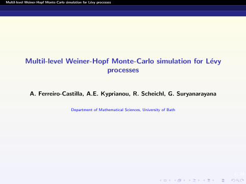
Multi-level Wiener-Hopf Monte-Carlo [Heinrich, 2001], [Giles, 2007], . . .

Computational gains from exploiting the telescopic sum

E[FnL ] = E[Fn0 ] +∑L

`=1E[Fn` − Fn`−1 ],

where n` = 2`n0, ` = 1, . . . ,L, for some small n0 ∈ N.

Suggesting the multilevel estimator

Fn0,L,{M`}ML :=

M0∑i=1

Fn0,(i) +

L∑`=1

M∑i=1

(Fn`,(i) − Fn`−1,(i)).

Here it is very important that Fn`−1 can be obtained from Fn` by a“deterministic” transformation of the random variables used to obtain Fn` .

A little algebra again reveals that the means square error satisfies

e(Fn0,L,{M`}ML )2 =

M0V(Fn0) +

L∑`=1

M`V(Fn` − Fn`−1) +

(E[Fn − F (X1,X 1)]

See also [Dereich, Heidenreich, 2011], [Dereich, 2011], [Giles, Xia, 2012].

17/ 24

E[FnL ] = E[Fn0 ] +∑L

`=1E[Fn` − Fn`−1 ],

Fn0,L,{M`}ML :=

M0∑i=1

Fn0,(i) +L∑`=1

M∑i=1

(Fn`,(i) − Fn`−1,(i)).

e(Fn0,L,{M`}ML )2 =

M0V(Fn0) +

L∑`=1

M`V(Fn` − Fn`−1) +

(E[Fn − F (X1,X 1)]

17/ 24

E[FnL ] = E[Fn0 ] +∑L

`=1E[Fn` − Fn`−1 ],

Fn0,L,{M`}ML :=

M0∑i=1

Fn0,(i) +L∑`=1

M∑i=1

(Fn`,(i) − Fn`−1,(i)).

e(Fn0,L,{M`}ML )2 =

M0V(Fn0) +

L∑`=1

M`V(Fn` − Fn`−1) +

(E[Fn − F (X1,X 1)]

17/ 24

E[FnL ] = E[Fn0 ] +∑L

`=1E[Fn` − Fn`−1 ],

Fn0,L,{M`}ML :=

M0∑i=1

Fn0,(i) +L∑`=1

M∑i=1

(Fn`,(i) − Fn`−1,(i)).

e(Fn0,L,{M`}ML )2 =

M0V(Fn0) +

L∑`=1

M`V(Fn` − Fn`−1) +

(E[Fn − F (X1,X 1)]

18/ 24

Poisson thinning and multilevel WHMC

In the WHMC method how do we introduce ”levels”?Recall also that it is crucial to have a Poisson process for the timerandomisations on all levels! How do we sample on two consecutive levels?

Suppose the ”level `” grid is based on a Poisson process of rate n`. Thenby tossing a coin and rejecting arrivals with probability 1/2 we end up witha Poisson process of rate n`−1: our new coarser ”level `− 1” Poisson grid.(Not a new idea! Also used by [Glasserman, Merener, 2003], [Giles, Xia, 2012], . . . )

18/ 24

In the WHMC method how do we introduce ”levels”?

Recall also that it is crucial to have a Poisson process for the timerandomisations on all levels! How do we sample on two consecutive levels?

18/ 24

19/ 24

Numerical Analysis (multilevel case)Theorem (Multilevel WHMC)

Assume ∃α, β > 0 with α ≥ 12

max{β, 1} such that

(i) |E[Fn` − F (Xt ,X t)]| . n−α`

(ii) V[Fn` − Fn`−1 ] . n−β`

(iii) E[Cn` ] . n`.

Then, ∀ν ∈ N ∃L and {M`}L`=0 s.t. C(F

n0,L,{M`}ML

). ν and L2 error

n0,L,{M`}ML

12 if β > 1 ,

ν−12 log2 ν if β = 1 ,

ν− 1

2+(1−β)/α if β < 1 .

For Kuznetsov’s β-class of Levy processes also Assumption (iii) holds.

Recall that α = (1/4)1/2 for (un)bounded variation paths & shortly we

shall see β = 1/2 ⇒ (O(ν−14 )) O(ν−

Compare with former (single-level) rates (O(ν−16 )) O(ν−

19/ 24

Numerical Analysis (multilevel case)Theorem (Multilevel WHMC)

Assume ∃α, β > 0 with α ≥ 12

max{β, 1} such that

(i) |E[Fn` − F (Xt ,X t)]| . n−α`

(ii) V[Fn` − Fn`−1 ] . n−β`

(iii) E[Cn` ] . n`.

Then, ∀ν ∈ N ∃L and {M`}L`=0 s.t. C(F

n0,L,{M`}ML

). ν and L2 error

n0,L,{M`}ML

12 if β > 1 ,

ν−12 log2 ν if β = 1 ,

ν− 1

2+(1−β)/α if β < 1 .

For Kuznetsov’s β-class of Levy processes also Assumption (iii) holds.

Recall that α = (1/4)1/2 for (un)bounded variation paths & shortly we

shall see β = 1/2 ⇒ (O(ν−14 )) O(ν−

Compare with former (single-level) rates (O(ν−16 )) O(ν−

20/ 24

Numerical analysis MLWH

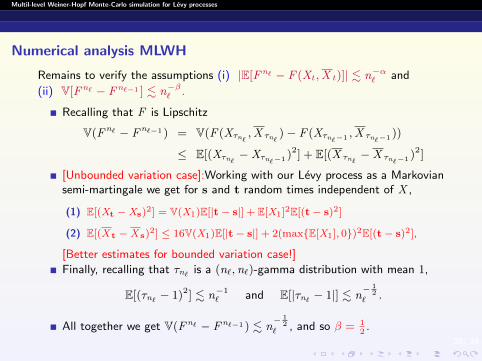
Remains to verify the assumptions (i) |E[Fn` − F (Xt ,X t)]| . n−α` and

(ii) V[Fn` − Fn`−1 ] . n−β` .

Recalling that F is Lipschitz

V(Fn` − Fn`−1) = V(F (Xτn` ,X τn`)− F (Xτn`−1 ,X τn`−1))

≤ E[(Xτn` −Xτn`−1)2] + E[(X τn`−X τn`−1)2]

[Unbounded variation case]:Working with our Levy process as a Markoviansemi-martingale we get for s and t random times independent of X ,

(1) E[(Xt −Xs)2] = V(X1)E[|t− s|] + E[X1]2E[(t− s)2]

(2) E[(X t −X s)2] ≤ 16V(X1)E[|t− s|] + 2(max{E[X1], 0})2E[(t− s)2],

[Better estimates for bounded variation case!]

Finally, recalling that τn` is a (n`,n`)-gamma distribution with mean 1,

E[(τn` − 1)2] . n−1` and E[|τn` − 1|] . n

− 12

All together we get V(Fn` − Fn`−1) . n− 1

2` , and so β = 1

Via Jensen’s inequality we then easily also get α = 14

20/ 24

(ii) V[Fn` − Fn`−1 ] . n−β` .

≤ E[(Xτn` −Xτn`−1)2] + E[(X τn`−X τn`−1)2]

E[(τn` − 1)2] . n−1` and E[|τn` − 1|] . n

− 12

2` , and so β = 1

20/ 24

(ii) V[Fn` − Fn`−1 ] . n−β` .

≤ E[(Xτn` −Xτn`−1)2] + E[(X τn`−X τn`−1)2]

E[(τn` − 1)2] . n−1` and E[|τn` − 1|] . n

− 12

2` , and so β = 1

20/ 24

(ii) V[Fn` − Fn`−1 ] . n−β` .

≤ E[(Xτn` −Xτn`−1)2] + E[(X τn`−X τn`−1)2]

E[(τn` − 1)2] . n−1` and E[|τn` − 1|] . n

− 12

2` , and so β = 1

20/ 24

(ii) V[Fn` − Fn`−1 ] . n−β` .

≤ E[(Xτn` −Xτn`−1)2] + E[(X τn`−X τn`−1)2]

E[(τn` − 1)2] . n−1` and E[|τn` − 1|] . n

− 12

2` , and so β = 1

21/ 24

Kuznetsov’s β-class

The characteristic exponent (Ψ(θ) = − logE(eiθX1), θ ∈ R) is given by

Ψ(θ) = iaz +1

2σ2z 2 +

{B(α1, 1− λ1)− B(α1 −

β1, 1− λ1)

}+c2β2

{B(α2, 1− λ2)− B(α2 +

β2, 1− λ2)

}where B(x , y) = Γ(x)Γ(y)/Γ(x + y) is the Beta function, with parameterrange a ∈ R, σ, ci , αi , βi > 0 and λ1, λ2 ∈ (0, 3) \ {1, 2}.The corresponding Levy measure Π has density

π(x) = c1e−α1β1x

(1− e−β1x )λ11{x>0} + c2

eα2β2x

(1− eβ2x )λ21{x<0}.

The β-class of Levy processes includes another recently introduced familyof Levy processes known as Lamperti-stable processes.

22/ 24

Meromorphic Levy processes (contains the β-class)

(i) The characteristic exponent Ψ(z ) is a meromorphic function which haspoles at points {−iρn , iρn}n≥1, where ρn and ρn are positive real numbers.

(ii) For q ≥ 0 function q + Ψ(z ) has roots at points {−iζn , iζn}n≥1 where ζnand ζn are nonnegative real numbers (strictly positive if q > 0). We willwrite ζn(q), ζn(q) if we need to stress the dependence on q .

(iii) The roots and poles of q + Ψ(iz ) satisfy the following interlacing condition

...− ρ2 < −ζ2 < −ρ1 < −ζ1 < 0 < ζ1 < ρ1 < ζ2 < ρ2 < ...

(iv) The Wiener-Hopf factors are expressed as convergent infinite products,

E[e−zXeq

]=∏n≥1

1 + zρn

1 + zζn

E[ezXeq

]=∏n≥1

1 + zρn

23/ 24

Distribution of extrema

For x ≥ 0

P(X eq ∈ dx) = a0(ρ, ζ)δ0(dx) +

∞∑n=1

an(ρ, ζ)ζne−ζnxdx

a0(ρ, ζ) = limn→+∞

n∏k=1

ζkρk, an(ρ, ζ) =

(1− ζn

)∏k≥1k 6=n

1− ζnρk

1− ζnζk

A similar expression holds for P(−X eq∈ dx).

24/ 24

References

Cliffe, K.A., Giles, M.B., Scheichl, R. and Teckentrup, A.L. (2011)Multilevel Monte Carlo methods and applications to elliptic PDEs withrandom coefficients. Comput. Visual. Sci. 14(1), 3–15.

Dereich, S. (2011) Multilevel Monte Carlo Algorithms for Levy–drivenSDEs with Gaussian correction. Ann. Appl. Probab. 21(1), 283–311.

Dereich, S. and Heidenreich, F. (2011) A multilevel Monte Carlo algorithmfor Levy–driven stochastic differential equations. Stochastic Process. Appl.121(7), 1565–1587.

Giles, M.B. (2008) Multilevel Monte Carlo Path Simulation. Oper. Res.56(3), 607–617.

Jacod, J., Kurtz, T.G., Meleard, S. and Protter, P. (2005) Theapproximate Euler method for Levy driven stochastic differential equations.Ann. Inst. H. Poincare Probab. Statist. 41, 523–558.

Kuznetsov (2010) Wiener-Hopf factorization and distribution of extremafor a family of Levy processes Ann. Appl. Probab. 20, 1801–1830.

Multil-level Weiner-Hopf Monte-Carlo simulation for Lévy ... · Multil-level Weiner-Hopf...

Documents

Transcript of Multil-level Weiner-Hopf Monte-Carlo simulation for Lévy ... · Multil-level Weiner-Hopf...